seasonal variation of turbulent energy dissipation rates ... · seasonal variation of turbulent...

Earth Planets Space, 51, 515–524, 1999

Seasonal variation of turbulent energy dissipation rates in the polar mesosphere:a comparison of methods

C. M. Hall1, U.-P. Hoppe2, T. A. Blix2, E. V. Thrane2, A. H. Manson3, and C. E. Meek3

1Department of Physics, University of Tromsø, 9037 Tromsø, Norway2Norwegian Defence Research Establishment, 2027 Kjeller, Norway

3Institute of Space and Atmospheric Studies, University of Saskatchewan, Saskatoon, Saskatchewan, Canada

(Received June 29, 1998; Revised January 20, 1999; Accepted June 3, 1999)

During the last two decades many estimates of turbulence strength have been made by a variety of techniquesin the mesosphere above northern Norway. We have assimilated many of these results and present them in thisstudy, enabling the reader to note systematic differences. We concentrate on seasonal variation not only in anattempt to smooth out non-representative data, but also to identify the seasonal features themselves. We note bothsemi-annual and annual variations in turbulent intensity, depending on the height considered. Finally we address theaforementioned systematic differences between the methods and suggest possible causes in terms of each method’sunderlying assumptions.

1. IntroductionIt is no coincidence that a broad spectrum of ground-based

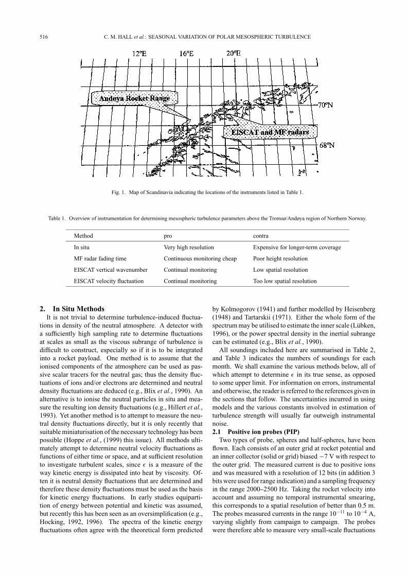
instrumentation has been built up in the vicinities of Andenesand Tromsø in Northern Scandinavia and furthermore in thevicinity of a sounding rocket launching facility (Fig. 1). Theavailable instrumentation has provided the scientific commu-nity with both ground-based and in situ measurements of themesosphere over a period of almost 2 decades and it is nowbecoming possible to study such data in a statistical way. Re-sults from ion-, electron- and neutral density probes, EISCAT(European Incoherent Scatter Radar) and the University ofTromsø/University of Saskatchewan MF radar system havebeen selected for this study. We shall address the turbulentenergy dissipation rate, ε, in this study. ε is a commonlyderived entity for parameterising turbulent intensity and iseasily converted to a heating rate in K/day, which is a conve-niently understandable unit. We have selected 4 basic meth-ods of estimating ε, the results from which we will presentand intercompare. We shall find agreement and disagreementbetween the methods and for the latter case briefly discussthe possible reasons. A paper by Hocking (1999) in this is-sue represents a critique of much of the theory underlyingthese derivations. For this reason we include commonly-used formulae in this paper to facilitate reference to Hocking(1999). Clearly, to identifywhy onewell-establishedmethodyields significantly different results from another is crucialto future research and not least, financial investment in newinstruments and observations. Furthermore, different meth-ods have advantages and disadvantages compared to others.A secondary object of this study is to help identify whichkind of observation is best suited to which kind of study. For

Copy right c© The Society of Geomagnetism and Earth, Planetary and Space Sciences(SGEPSS); The Seismological Society of Japan; The Volcanological Society of Japan;The Geodetic Society of Japan; The Japanese Society for Planetary Sciences.

example, high spatial-resolution case-study kinds of mea-surements are best performed in situ; while studies of diurnalvariations would be expensive using rockets, ground-basedexperiments are perhaps better suited for this purpose. MFradar systems are relatively cheap to build but often sufferfrom poor height resolution. In addition, they are often af-fected by group delay of the radio wave by the ionosphere,and so the exact heights of the observations can be uncertainabove 90 km. Perhaps an even more important contaminantis the leading edge of any very large E-region echo “leaking”into theMF data at∼92 km and above (Hocking, 1997). Themethods we shall describe in more detail below are tabulatedalongwith themain advantages and disadvantages in Table 1.We should stress that the table is indicating which method isbest suited to a particular kind of observation, not that one ormore methods should be discarded altogether. Furthermore,it is important to note that while some methods attempt toestimate the turbulent energy dissipation rate itself, othersrather determine an upper limit for it. Differences betweenthe “upper-limit” estimates and the actual energy dissipationrate characterising the inertial subrange of turbulence arisefrom processes that “violate” the classical energy cascade.Also, we shall see that many methods employ a length scale,often an estimated “outer scale” (or largest scale enjoyed byinertial processes); buoyant dynamics smaller in scale thanthis estimate will also cause derived dissipation rates to belarger than the purely turbulent energy disspation rate.Throughout the forthcoming descriptions of the various

methods, we need to employ values for the Brunt-Vaisalafrequency; we normally take this from theMSISE90 (Hedin,1991) model temperatures which offer good continuity inboth time and height. Where previously published data hasbeen included, other models and/or measurements may havebeen used and these are either quoted in the text or availablevia the corresponding reference.

515

516 C. M. HALL et al.: SEASONAL VARIATION OF POLAR MESOSPHERIC TURBULENCE

Fig. 1. Map of Scandinavia indicating the locations of the instruments listed in Table 1.

Table 1. Overview of instrumentation for determining mesospheric turbulence parameters above the Tromsø/Andøya region of Northern Norway.

Method pro contra

In situ Very high resolution Expensive for longer-term coverage

MF radar fading time Continuous monitoring cheap Poor height resolution

EISCAT vertical wavenumber Continual monitoring Low spatial resolution

EISCAT velocity fluctuation Continual monitoring Too low spatial resolution

2. In Situ MethodsIt is not trivial to determine turbulence-induced fluctua-

tions in density of the neutral atmosphere. A detector witha sufficiently high sampling rate to determine fluctuationsat scales as small as the viscous subrange of turbulence isdifficult to construct, especially so if it is to be integratedinto a rocket payload. One method is to assume that theionised components of the atmosphere can be used as pas-sive scalar tracers for the neutral gas; thus the density fluc-tuations of ions and/or electrons are determined and neutraldensity fluctuations are deduced (e.g., Blix et al., 1990). Analternative is to ionise the neutral particles in situ and mea-sure the resulting ion density fluctuations (e.g., Hillert et al.,1993). Yet another method is to attempt to measure the neu-tral density fluctuations directly, but it is only recently thatsuitableminiaturisation of the necessary technology has beenpossible (Hoppe et al., (1999) this issue). All methods ulti-mately attempt to determine neutral velocity fluctuations asfunctions of either time or space, and at sufficient resolutionto investigate turbulent scales, since ε is a measure of theway kinetic energy is dissipated into heat by viscosity. Of-ten it is neutral density fluctuations that are determined andtherefore these density fluctuations must be used as the basisfor kinetic energy fluctuations. In early studies equiparti-tion of energy between potential and kinetic was assumed,but recently this has been seen as an oversimplification (e.g.,Hocking, 1992, 1996). The spectra of the kinetic energyfluctuations often agree with the theoretical form predicted

by Kolmogorov (1941) and further modelled by Heisenberg(1948) and Tartarskii (1971). Either the whole form of thespectrummay be utilised to estimate the inner scale (Lubken,1996), or the power spectral density in the inertial subrangecan be estimated (e.g., Blix et al., 1990).All soundings included here are summarised in Table 2,

and Table 3 indicates the numbers of soundings for eachmonth. We shall examine the various methods below, all ofwhich attempt to determine ε in its true sense, as opposedto some upper limit. For information on errors, instrumentaland otherwise, the reader is referred to the references given inthe sections that follow. The uncertainties incurred in usingmodels and the various constants involved in estimation ofturbulence strength will usually far outweigh instrumentalnoise.2.1 Positive ion probes (PIP)Two types of probe, spheres and half-spheres, have been

flown. Each consists of an outer grid at rocket potential andan inner collector (solid or grid) biased −7 V with respect tothe outer grid. The measured current is due to positive ionsand was measured with a resolution of 12 bits (in addition 3bitswere used for range indication) and a sampling frequencyin the range 2000–2500 Hz. Taking the rocket velocity intoaccount and assuming no temporal instrumental smearing,this corresponds to a spatial resolution of better than 0.5 m.The probes measured currents in the range 10−11 to 10−4 A,varying slightly from campaign to campaign. The probeswere therefore able to measure very small-scale fluctuations

C. M. HALL et al.: SEASONAL VARIATION OF POLAR MESOSPHERIC TURBULENCE 517

Table 2. Details of rocket soundings used in this paper. Further details canbe found via the references given in the text along with the designationgiven in the first column.

Rocket designation Launch date and time

F-52 PIP 11 Nov. 1980 03:24 1

F-53 PIP 16 Nov. 1980 03:31 1

F-54 PIP 11 Nov. 1980 00:12 1

F-55 PIP 16 Nov. 1980 03:31 1

F-56 PIP 28 Nov. 1980 03:24 1

F-56 PIP 28 Nov. 1980 03:24 1

F-56 PIP 28 Nov. 1980 03:24 1

F-56 PIP 28 Nov. 1980 03:24 1

F-57 PIP 11 Nov. 1980 00:12 1

F-57 PIP 11 Nov. 1980 00:12 1

F-64 PIP 16 Feb. 1984 01:20 2

F-65 PIP 18 Feb. 1984 00:22 2

F-66 PIP 6 Jan. 1984 21:55 2

F-67 PIP 25 Jan. 1984 17:39 2

F-68 PIP 13 Jan. 1984 20:00 2

F-69 PIP 10 Feb. 1984 02:40 2

F-70 PIP 31 Jan. 1984 18:31 2

F-74 PIP 12 Nov. 1987 00:16 3

F-75 PIP 21 Oct. 1987 21:33 3

F-76 PIP 15 Oct. 1987 10:52 3

F-77 PIP 21 Oct. 1987 21:33 3

F-78 PIP 12 Nov. 1987 00:21 3

F-81 PIP and TOTAL 22 Jan. 1990 10:20 4

F-82 PIP and TOTAL 25 Feb. 1990 19:20 5

F-83 PIP and TOTAL 6 Oct. 1990 02:41 5

F-84 PIP and TOTAL 8 Mar. 1990 22:53 5



F-90 TOTAL 1 Aug. 1991 01:40 6

F-91 PIP and TOTAL 9 Aug. 1991 23:15 6

F-95 PIP and TOTAL 17 Sept. 1991 23:43 7


F-93 TOTAL 20 Aug. 1991 22:40 7




F-100 CONE 28 Jul. 1993 22:23 8

F-94 PIP and CONE 1 Aug. 1993 01:46 8

F-102 CONE 28 Jul. 1993 22:39 9

F-103 CONE 31 Jul. 1993 00:50 9

F-101 PIP and CONE 1 Aug. 1993 00:53 9

Super Arcas 1 NTP 14 Jul. 1987 08:00 10




1Energy Budget Campaign, 2MAP/WINE, 3MAC/EPSILON,4Recommend, 5DYANA, 6NLC-91, 7METAL, 8SCALE, 9ECHO,10MAC/SINE.

Table 3. Numbers of soundings used to obtain each of the month averagesdescribed in the text.

Month Number of soundings

January 7

February 6

March 11

April 0

May 0

June 0

July 7

August 6

September 9

October 9

November 13

December 0

(down to 0.02%) with high spatial resolution in the middleatmosphere.Wewill, below, describe howwehave treated the data from

the different soundings performed during the years (1980–1994). The aim has been to treat all data in a consistentmanner so that they can be directly compared and used asthe basis for the annual variations discussed later. Earlyrocket sounding data analyses employed the US Standardatmosphere (NOAA-S/T76-1562, 1976), to obtain neutralatmosphere scale heights for pressure (Hp) and density (Hn),and we have used the same throughout for consistency. Thescale height of the ion density (Hi) has been derived directlyfrom the ion probe data. The significance of these parametersis obvious from the following discussion.If the original telemetry data were available (soundings

from 1990 onwards) we have performed the analysis de-scribed in detail by Thrane et al. (1985), again including anycompensation for negative ions. For each sounding (uplegand/or downleg) we assembled one-kilometre altitude timeseries (cf. Blix et al.’s (1990) 1024 points). Having obtainedsets of well behaved time series, a digital filter was appliedgiving a bandpass from 4Hz (rejecting the spin frequency) toaround 60 Hz, corresponding to 15 m. The variances of theresults were then converted to neutral density fluctuations,�n/n, according to the method of Blix et al. (1990). Thecorresponding potential energy (per unit mass) fluctuationPE′ is derived from

PE′ = zg�n

n(1)

where z is the vertical displacement of an air parcel. Assum-ing adiabatic vertical displacement of air parcels, Thrane andGrandal (1981) found the following relation between �n/nand z:

�n

n=

[1

Hn− 1

γ Hp

]z (2)

where Hn and Hp are the neutral density and pressure scale


heights respectively. This expression is very similar to equa-tion 17 of Hocking (1985) except that in this case scaleheights are used whereas Hocking used gradients. The spe-cific (kg−1) kinetic energy fluctuation KE′ = 1

2U2, U being

the turbulent velocity. U can be related to the horizontal (uand v) and vertical (w) components asU 2 = u2+v2+w2 =Cw2, where C is constant describing the degree of isotropy.Thus, KE′ = C · 1

2w2. The relation between KE′ and PE′ is

given by the equation:

KE′ = PE′[(1 − Ri)/Ri] (3)

(Weinstock, 1978; Hocking, 1992). We have taken Ri =0.44, this being suggested by (Weinstock, 1978) as a valuerepresentative of established andmaintained turbulence. Therelation (3) above is valid for 0 < Ri ≤ 1 (see Hocking(1992) for further details). It is unlikely, however, that onecan characterise the atmosphere with any single value of Ri;see Hocking and Mu (1997) for a more detailed discussion,including variations on Eq. (3) in terms of flux RicharsonNumber. The w2 derivation of ε is then given by

ε = 0.4w2ωB = 0.8KE′ωB/C (4)

ωB being the Brunt-Vaisala frequency. We have assumedisotropic turbulence (C = 3) in our derivation of ε. Onemust be careful about adopting the factor 3 however; theremay be additional re-scaling constants of the order of 4/3depending on whether w fluctuations are measured parallelor perpendicular to the motion of the detector through theturbulence.If the original telemetry data were unavailable (prior to

1990), we have taken the published profiles of ε (all appro-priate references can be found in Blix et al. (1990)), andconverted them to profiles of neutral density fluctuation byexactly reversing the process described in detail by Blix etal. (1990). First, we obtain the structure function constantC2n using:

C2n = (ε/0.293)2/3B[M/ωB]2 (5)

where M = (γ Hp/Hn − 1)/γ Hp. Here, B is a factor de-scribed by Blix et al. (1990) giving the relation between hor-izontal and vertical gradients. B = 3 corresponds to the casethat fluctuations at scales greater than LB , the outer scale, areisotropic. B = 1 corresponds to the case that scales greaterthan LB are stratified. Scales smaller than LB and in theinertial subrange are actually isotropic in both cases. Forconsistency with other results we shall incorporate, we havechosen to use B = 3 in accordance with Blix et al. (1990)in our derivation. Then we obtain the power spectral densityP( f ) at frequency f0 from:

C2n = 8Pn( f )(2π/VR)2/3 f 5/30 (6)

where VR is the rocket velocity and choosing a frequencyf0 in the range 4–60 Hz. Since the power spectrum P( f )depends upon the frequency as f −5/3 in the inertial sub-range, we can then integrate the power spectrum over thefrequency range 4–60 Hz described above to obtain �n/n.From thereon we can use the previous equations (1)–(4) toderive ε in a consistent manner. In each case, the ε profileswere then corrected for negative ion presence as described by

Hall (1997a). The correction has negligible consequences ifthe turbulence was significant. This is because one effect ofthe negative ions is to introduce a narrow viscous-convectivesubrange, and this will contribute relatively little if the iner-tial subrange is large; the reader is referred to Hall (1997a)for estimates of the magnitudes of negative ion effects.2.2 Ionisation gauge (TOTAL/CONE)The TOTAL and CONE instruments have been discussed

in the literature and we will therefore only give the mostimportant information here. Both instruments are in prin-ciple ionisation gauges measuring the neutral density andneutral density fluctuations with high precision (instrumen-tal noise less than 0.1% of the total signal) and resolution(better than a few metres). The basic difference betweenthe two instruments is that TOTAL is closed while CONEis an open ionisation gauge. The latter is much less influ-enced by the flow round the instrument and is therefore notas sensitive to ram (aerodynamic sense) effects. The neutraldensity fluctuations have been used to derive energy dissipa-tion rates following the method outlined by Lubken (1996)and Lubken et al. (1993) and will not be repeated here. Thebasic principle of the method is to use the power spectrum ofthe observed density fluctuations and a theoretical model toobtain the best fit to the spectrum (see Lubken et al. (1993)for further details). From this fit, the inner scale l0 indicat-ing the transfer from the inertial to viscous subranges in thespectrum and hence the energy dissipation rate ε is obtained.Although this method does not directly estimate the kineticenergy spectrum, thematter of partition of energy is nonethe-less implicit in the theoretical spectrum to which the data arefitted. The estimation of ε depends on the relation between η,the Kolmogorov microscale and l0, the inner scale, and thisis often given by l0 = C4η. Lubken et al. (1993) show howC4 may be 9.9 using the formulation of Heisenberg (1948),or 7.06 using that of Tartarskii (1971). Specifically, for theformer:

C4 = l0/η = 2π{9 fαa2�(5/3) sin(π/3)

16 Prmoln

}3/4

. (7)

Here Prmoln is the molecular Prandtl number; fα is a factor

equal to either 1 or 2 accounting for different nomalisationsof the rate at which inhomogeneity is removed by molec-ular diffusion; a2 is an experimentally determined constant(which we shall discuss later). It is from the spectral deter-mination of l0 combined with Eq. (7) and

η =(

ν3

ε

)1/4

(8)

ν being the kinematic viscosity (a function of both densityand temperature), that we may determine ε.2.3 Nose tip probe (NTP)The nose tip probemeasuring electron density fluctuations

has been discussed by, for example, Ulwick et al. (1988). Theprobe consists of an isolated tip (about 4 cm in length) of thenose cone of the rocket and is held at a fixed potential of+3 V with respect to the rocket skin. The data were sam-pled at 8000Hz giving an effective height resolution of betterthan 1 m. Energy dissipation rates ε were derived using theso-called C2

n -method described above and for example by


Blix et al. (1990) using spectra of electron density fluctua-tions as input. The data employed here have previously beenpublished by Kelley et al. (1990).

3. MF Radar Signal Fading Time MethodWe may illuminate the mesosphere and lower thermo-

sphere using an MF radar. Structures in the electron den-sity, at heights and times where the atmosphere is ionised tosome degree, may give rise to sharp gradients in the refractiveindex at the transmitted frequency. These gradients scatterradiation (by either partial reflection or volume scatter) toform an interference pattern on the ground. Spaced antennaedetect the movement of this pattern (moving with twice thespeed of the scatterers), giving indications of the horizontalwind. In addition, however, the signals fade due to the scat-terer motion (both uniform and fluctuating) and dissipationof the scatterers. The fluctuating component of the motion isused to estimate turbulent strength: the characteristic fadingtime may be related to the eddy diffusivity and hence the tur-bulent energy dissipation rate. This kind of measurement isdescribed by Hocking (1997) who describe other methods,and compare with this one. The details of the method ofcorrelating the signals from each of the spaced receivers areaddressed by Briggs (1984), and the method is commonlyreferred to as the Full Correlation Analysis (FCA).Descriptions of the experimental set up of the joint Univer-

sity of Tromsø/University of SaskatchewanMF radar may befound via Hall et al. (1998). The signal fading times, τc, andvelocity fluctuations, v′, appropriate to an observer movingwith the backgroundwind, are computed according to Briggs(1984). In particular, and as used by Hall et al. (1998), at aheight resolution of 3 km and time resolution of 5 minuteswe use:

v′ = λ√ln 2

4πτc(9)

where λ is the radar wavelength. The energy dissipationrate may be arrived at by dividing the kinetic energy of theturbulence, related to v′2, by a timescale (Blamont, 1963).In previous studies, (e.g., Manson et al., 1981) the Brunt-Vaisala period has been identified as a suitable timescale, thefluctuation as the vertical component, w, and the expressionε = 0.4w2ωB has been used (ωB being the Brunt-Vaisalafrequency). If we derived the velocity variance by a line-of-sightDopplermeasurement the expressionwould be differentas described exactly by Hocking (1983). Here, however,we have assumed that all three components of the velocityfluctuation are responsible for the fading of the signal andhave thus chosen to use

ε′ = 0.8v′2/TB (10)

(Hall et al., 1998) where TB is the Brunt-Vaisala period inseconds. Note that we recognise that the spatial scale inher-ent in the experiment cannot preclude buoyancy-scale fluc-tuations, because the outer scale of turbulence, LB can beexpected to be as little as 200 m in the mesosphere. Thereis a very real danger of gravity wave contamination thatwould lead to overestimates of ε, the consequences for bothspectral-width and velocity-fluctuation based methods be-ing addressed by Hocking (1996). We therefore choose to

introduce ε′ to distinguish our estimate from ε. To use a for-mulation for ε which assumes a radar completely free frombeam broadening here would have been clearly inappropri-ate. We have therefore attempted to address the warningsof Hocking (1983) (somewhat weakened by Vandepeer andHocking (1993)) by accepting that v′ is an estimate of to-tal velocity perturbations within the scattering volume andchoosing a time scale accordingly. We have attempted tojustify this philosophy by checking for correlation betweenthe estimates of ε′ and the total wind amplitude: a clear cor-relation might be anticipated if beam-broadening was signif-icantly enhancing our estimate, which was not the case (Hallet al., 1998).

4. EISCAT-Derived Characteristic VerticalWave-number Method

TheEISCAT (Baron, 1984) radar atRamfjordmoen (69◦N,19◦E) in Northern Scandinavia is periodically run in a modeoptimised for the mesosphere (Collis and Rottger, 1990).Data from thismode includes vertical soundings of the heightrange 70–90 kmand results aremade availablewhich provideestimates of the vertical component of the neutral air motion(Collis, 1987). The time resolution is 5 minutes and theheight resolution 1.05 km. The data incorporated in thisstudy are summarised in Table 4.A typical EISCAT dataset giving vertical velocities over

a total interval of 112 days might exhibit broad regions of

alternate upward and downward motion due to tides, semi-and terdiurnal being common modes; these are invariablymodulated by the shorter period motions of gravity waves—sometimes showing very clearly, but often displaying a quasi-chaotic nature due to superposition of many periodicities.Furthermore, operations may be interrupted by transmitterand other failures. Low signal-to-noise ratios, particularlyduring geomagnetically quiet conditions at night and at lowaltitudes, impair extraction of Doppler shifts from the inco-herent scatter spectra. We shall see how consequences ofthese problems are minimised in the vertical wavenumbermethod that follows. The consequences are direr for thevelocity fluctuation method outlined in Section 5.In order to tolerate intermittent data, spectral analyses are

performed on the time-height data arrays using the Lomb-Scargle method described by Press and Rybicki (1989). Thismethod is particularly useful for our purposes because notonly is it designed for irregularly spaced data, but it yieldsboth a characteristic frequency (the wavenumber, m∗, in ourcase) and the significance that this is a true periodicity andnot noise. For each timestep, we determine the periodogramincluding all available dynamics scales and then its character-istic wavenumber and significance. These spectra and theircharacteristic wavenumbers exhibiting a 95% confidence areaveraged together. The average characteristic wavenumber,which represents gravity waves, is taken to be equivalent tothe m∗ as defined in Fritts and van Zandt (1993). An obvi-ous disadvantage in our strategy is that we are only obtainingan average for the height range 70–90 km (indeed, the databetween 70 and 75 km tends to be sparse). According toFritts and van Zandt (1993) this determination of ε should infact be regarded as an upper limit (Fritts, private communi-cation) in the same way as for the MFmethod just described.


Table 4. Dates of EISCAT experiments and numbers of 95% confidence m∗ samples as used in this study. Also included are the average m∗ values (m−1)and vertical velocity variances (m−2s−2) for each period.

Date No. of samples m∗ (m−1) Variance (m−2s−2)

12 June 1990 116 6.16E-05 2.76223

30 July 1990 97 5.53E-05 3.98875

27 August 1990 5 6.52E-05 1.4654

12 February 1991 4 5.33E-05 3.0578

20 February 1991 2 5.19E-05 5.74342

17 March 1991 55 5.97E-05 1.50099

4 June 1991 149 5.68E-05 1.74011

10 July 1991 84 5.87E-05 3.48824

10 June 1992 7 5.57E-05 6.21632

30 July 1992 299 5.79E-05 4.37461

27 October 1992 25 6.22E-05 2.08728

20 January 1993 33 5.14E-05 7.37154

15 June 1993 49 5.65E-05 2.90204

20 July 1993 7 5.37E-05 6.28883

14 September 1993 14 6.58E-05 0.654379

15 March 1994 68 6.23E-05 1.90955

11 August 1994 27 5.51E-05 3.05667

2 May 1995 322 6.66E-05 1.93373

17 December 1996 30 4.89E-05 5.92427

The advantage of this method is its robustness against uncer-tainties in vertical velocity for two reasons: (a) we only usesignificant periodicities, excluding random variations due toinstrument noise, and (b) awhite noise backgroundwould notbe expected to change the characteristic vertical wavelengthappreciably.Given an estimate ofm∗, Fritts and van Zandt (1993) then

give the total gravity wave energy as:

E0 = ω2B

10m2∗(11)

wherein we use the value of the Brunt-Vaisala frequency,ωB, given by Fritts and van Zandt (1993) for consistency.Similarly, and with reference again to Fritts and van Zandt,we define the energy scale height HE = 2.3H (H = 6.3 km)and so finally:

ε′ ≈ ωBE0

18m∗

(1

H− 3

2HE

)(12)

hence we obtain estimates for an upper limit of energy dissi-pation, which we again denote by ε′. From the above equa-tions, we can see that a 10% change in ωB would correspondto a 30% change in ε′. The sensitivity to HE is less, a 10%change here corresponding to a 10% change in ε′. Theseare acceptable if one notes that considerable notoriety in es-timates of ε′ stem from order of magnitude disagreementsbetween instruments, methods and interpretations.

5. EISCAT-Derived Vertical Velocity FluctuationMethod

The experiment description from the previous section ap-plies also to this method. Here a very simplistic approach isused by Hall (1997b) that avoids entailing any model atmo-sphere. The assumptions are simple to comprehend, but atthe same time raise the question as to viability. We simplytake adjacent determinations of the vertical velocity (recallthe EISCAT height resolution for the experiment in ques-tion is 1.05 km) and assume the difference to be the velocityfluctuation corresponding to an approximately 1 km eddy.Clearly, if the outer scale is only 200 m, for example, it is un-reasonable to talk of turbulence, and soHall (1997b) refers tothe resulting entity as a kilometer-scale kinetic energy fluc-tuation, ε1km:

ε1km(z) =[w(z, t) − w(z + 1050, t)

]3/1050 (13)

where w(z, t) is the vertical velocity at height z and time t .Here we have introduced yet another kind of energy dissipa-tion rate, which one should think of as an overestimate due toan imposed length scale. In the other ground-based methodsdescribed here, an upper limit is calculated with premedi-tated use of assumptions. The velocity fluctuation methodwas inspired by the work of Blamont (1963) in which suchfluctuations and their approximations to various definitionsof structure function are discussed in depth. Blamont (1963)


Fig. 2. In situ results. The soundings listed in Table 2 have been analysed using the methods described in the text. From Table 3 we note that no data wasavailable for April, May, June or December; the December profile is an average of the November and January profiles; the spring/early summer data isreplaced by the kinematic viscosity multiplied by the square of the Brunt-Vaisala frequency, this representing a minimum value of ε (e.g., Lubken et al.,1993). Units on the contours are in mWkg−1. Months with missing data are denoted by lighter shading.

furthermore illustrates an excellent description of the theoryby application to sodium cloud observations.

6. ResultsAll the methods described above yield profiles of “ε” as

functions of season, but with the exception of the characteris-tic wavenumber approach. Figures 2–4 present results fromeach of the first three methods. Note that the scales differsomewhat, but to allow for this, the contour levels have beenlabelled.For the in situ results for the months of April, May and

June, the expression εmin = ν · ω2B has been used, ν being

the kinematic viscosity, (e.g., Lubken et al., 1993) (cf. Eq.(14)). December, representing only a one-month gap, is theaverage of January andNovember. Subsequently a 3×3pointboxcar smoothing has been applied to the original resolutionsof 1 month and 1 km (Fig. 2).TheMF fading timemethod yields daily profiles eachwith

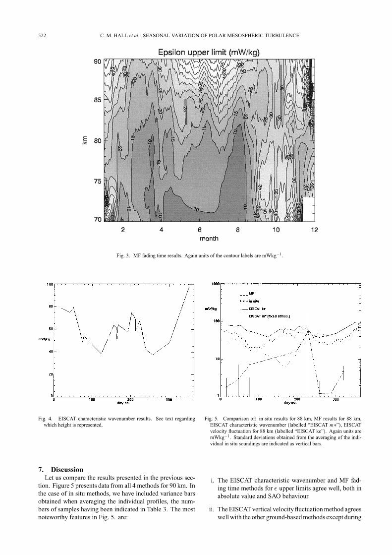
a 3 km height resolution. We show the data for 1997 here inFig. 3. Due to transmitter problems, January data has beenomitted. A one-week boxcar smoothing was applied.The characteristic vertical wavenumber method has pro-

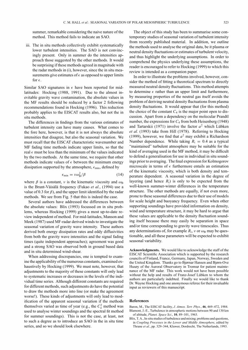
vided values of ε′ each of which is an average of typically1–2 days. The points are plotted according to date, ignoringthe year, and no smoothing has been used (Fig. 4). As wesee, the characteristic wavenumber method yields a simpletime series; each value is derived from a profile of vertical ve-locities, but not all measurement heights yield reliable data.We find that the average height (eachm∗ is associated with a

representative height depending on the useable velocity val-ues, and these representative heights may then be averaged)is around 79–80 km.The vertical velocity fluctuation method yields profiles

at each of the dates the characteristic vertical wavenumbermethod did. Since we feel that this method was rather anexploratory foray into the use of EISCAT to investigate tur-bulence we prefer not to present such results explicitly here.Let us now review the salient points of these figures:

i. Estimates of ε from in situ measurements (Fig. 2) re-veal an annual variation below 85 km with almost noturbulence in summer and almost constant turbulencewith height in winter. Above 85 km there is weak ev-idence for a semi-annual variation, although the clearfeature is the presence of strong turbulence at 89 km inlate summer.

ii. The MF results (Fig. 3) show relatively low turbulencelevels in the spring and summer, and a more even distri-bution of turbulence with height in winter. Thus, below80 km there is an annual variation. Above 80 km asemi-annual oscillation (SAO) signature is quite obvi-ous. Minima at the equinoxes have also been reportedby Hocking (1988, 1991).

iii. The characteristic vertical wavenumber method (Fig. 4)exhibits a clear SAO signature again similar to the find-ings reported by Hocking (1988, 1991).


Fig. 3. MF fading time results. Again units of the contour labels are mWkg−1.

Fig. 4. EISCAT characteristic wavenumber results. See text regardingwhich height is represented.

7. DiscussionLet us compare the results presented in the previous sec-

tion. Figure 5 presents data from all 4 methods for 90 km. Inthe case of in situ methods, we have included variance barsobtained when averaging the individual profiles, the num-bers of samples having been indicated in Table 3. The mostnoteworthy features in Fig. 5. are:

Fig. 5. Comparison of: in situ results for 88 km, MF results for 88 km,EISCAT characteristic wavenumber (labelled “EISCAT m∗”), EISCATvelocity fluctuation for 88 km (labelled “EISCAT ke”). Again units aremWkg−1. Standard deviations obtained from the averaging of the indi-vidual in situ soundings are indicated as vertical bars.

i. The EISCAT characteristic wavenumber and MF fad-ing time methods for ε upper limits agree well, both inabsolute value and SAO behaviour.

ii. TheEISCATvertical velocityfluctuationmethod agreeswellwith the other ground-basedmethods except during


summer, remarkable considering the naive nature of themethod. This method fails to indicate an SAO.

iii. The in situ methods collectively exhibit systematicallylower turbulent intensities. The SAO is not convinc-ingly present. Only in summer do the intensities ap-proach those suggested by the other methods. It wouldbe surprising if these methods agreed inmagnitude withthe radar methods in (i), however, since the in situ mea-surements give estimates of ε as opposed to upper limitsfor ε.

Similar SAO signatures in ε have been reported for mid-latitudes: Hocking (1988, 1991). Due to the almost in-evitable gravity wave contamination, the absolute values inthe MF results should be reduced by a factor 2 followingrecommendations found in Hocking (1996). This reductionprobably applies to the EISCAT results also, but not the insitu methods.The differences in findings from the various estimates of

turbulent intensity can have many causes. What comes tothe fore here, however, is that it is not always the absoluteintensities that disagree, but also the seasonal variation. Wemust recall that the EISCAT characteristic wavenumber andMF fading time methods indicate upper limits, so that thereal ε must be less than the minimum of the values indicatedby the two methods. At the same time, we require that othermethods indicate values of ε between the minimum energydissipation supported by the atmosphere, εmin, defined by

εmin = νω2B/β (14)

where β is a constant, ν is the kinematic viscosity and ωB

is the Brunt-Vaisala frequency (Fukao et al., (1994) use avalue of 0.3 for β), and the upper limit identified by the radarmethods. We see from Fig. 5 that this is indeed the case.Several authors have addressed the differences between

the absolute values: Blix (1993) focussed on in situ prob-lems, whereas Hocking (1999) gives a most up-to-date re-view independent of method. For mid-latitudes, Manson andMeek (1987) used MF-radar derived winds to investigate theseasonal variation of gravity wave intensity. These authorsderived both energy dissipation rates and eddy diffusivitiesfrom both the gravity wave intensities and the signal fadingtimes (quite independent approaches); agreement was goodand a strong SAO was observed both in ground based dataand in situ determined wind-shear.When addressing discrepancies, one is tempted to exam-

ine the applicability of the numerous constants, examined ex-haustively by Hocking (1999). We must note, however, thatadjustments to the majority of these constants will only leadto systematic increases or decreases in the levels of the indi-vidual time series. Although different constants are requiredfor different methods, such adjustments do have the potentialto draw the methods more into line (or make the agreementworse!). These kinds of adjustments will only lead to mod-ification of the apparent seasonal variation if the methodsthemselves varied as time of year (e.g., the C2

n method wasused to analyse winter soundings and the spectral fit methodfor summer soundings). This is not the case, at least, notto such a degree as to introduce an SAO in the in situ timeseries, and so we should look elsewhere.

The object of this study has been to summarise some con-temporary studies of seasonal variation of turbulent intensityfrom recently published material. In addition, we outlinethe methods used to analyse the original data, be it plasma orneutral density fluctuations or estimates of turbulent velocity,and thus highlight the underlying assumptions. In order tocomprehend the physics underlying these assumptions, thereader is encouraged to refer to Hocking (1999) to which thisreview is intended as a companion paper.In order to illustrate the problems involved, however, con-

sider the method of fitting a theoretical spectrum to directlymeasured neutral density fluctuations. This method attemptsto determine ε rather than an upper limit and furthermore,by measuring properties of the neutral gas itself avoids theproblem of deriving neutral density fluctuations from plasmadensity fluctuations. It would appear that (for this method)the choice of the constant C4 is the major point open to dis-cussion. Apart from a dependency on the molecular Prandtlnumber, the expressions forC4 from both Heisenberg (1948)and Tartarskii (1971) involve the factor a2 which Lubkenet al. (1993) take from Hill (1978). Referring to Hocking(1999), however, we find that a2 may exhibit a RichardsonNumber dependence. While taking Ri = 0.4 as a typical“maintained” turbulent atmosphere may be suitable for thekind of averaging used in the MF method, it may be difficultto defend a generalisation for use in individual in situ sound-ings prior to averaging. The final expression for Kolmogorovmicroscale in terms of ε furthermore entails an estimationof the kinematic viscosity, which is both density and tem-perature dependent. A seasonal variation in the degree oflayering (and hence Ri) is only to be expected from thewell-known summer-winter differences in the temperaturestructure. The other methods are equally, if not even more,prone to these seasonal differences due to their use of modelsfor scale height and buoyancy frequency. Even when othersupporting soundings have provided information on density,wind and temperature structure, it may be hard to argue thatthese values are applicable to the density fluctuation sound-ing itself because there may easily be separation in spaceand/or time corresponding to gravity wave timescales. Thusany determinations of, for example Ri, ν or ωB may be ques-tionable, and all these parameters will be expected to exhibitseasonal variability.

Acknowledgments. Wewould like to acknowledge the staff of theEISCAT Scientific Association which is supported by the researchcouncils of Finland, France, Germany, Japan, Norway, Sweden andthe United Kingdom. Thanks go to Bjørnar Hansen and Bjørn-OveHusøy of the Auroral Observatory in Tromsø for patient mainte-nance of the MF radar. This work would not have been possiblewithout the help and results of Franz-Josef Lubken to whom theauthors are particularly indebted. Finally we would like to thankDr.Wayne Hocking and one anonymous referee for their invaluableinput as reviewers of this manuscript.

ReferencesBaron, M., The EISCAT facility, J. Atmos. Terr. Phys., 46, 469–472, 1984.Blamont, J.-E., Turbulence in atmospheric motions between 90 and 130 km

of altitude, Planet. Space Sci., 10, 89–101, 1963.Blix, T.A., In-situ studies of turbulence andmixing; problems and questions,

in Coupling Processes in the Lower and Middle Atmosphere, edited byThrane et al., pp. 329–344, Kluwer, Dordrecht, The Netherlands, 1993.


Blix, T. A., E. V. Thrane, and Ø. Andreassen, In Situ Measurements of thefine-scale structure and turbulence in the mesosphere and lower thermo-sphere by means of electrostatic ion probes, J. Geophys. Res., 95(D5),5533–5548, 1990.

Briggs, B. H., The analysis of spaced sensor records by correlation tech-niques, Handb. MAP, 13, 166–186, 1984.

Collis, P. N., Common program data analysis at EISCAT, in Proceedings ofthe EISCAT Annual Review Meeting, Skibotn, Norway 2–5March, 1987,edited by P. N. Collis, 1987.

Collis, P. N. and J. Rottger, Mesospheric studies using the EISCATUHF andVHF radars: a review of principles and experimental results, J. Atmos.Terr. Phys., 52, 569–584, 1990.

Fritts, D. C. and T. E. van Zandt, Spectral estimates of gravity wave energyand momentum fluxes, J. Atmos. Sci., 50, 3685–3694, 1993.

Fukao, S., M. D. Yamanaka, N. Ao, W. K. Hocking, T. Sato, M. Yamamoto,T. Nakamura, T. Tsuda, and S. Kato, Seasonal variability of vertical eddydiffusivity in the middle atmosphere, 1. Three-year observations by themiddle and upper atmosphere radar, J. Geophys. Res., 99, 18,973–18,987,1994.

Hall, C.M., The influence of negative ions onmesospheric turbulence tracedby ionisation: implications for radar and in situ experiments, J. Geophys.Res., 102, 439–443, 1997a.

Hall, C. M., Kilometer scale kinetic energy perturbations in the mesospherederived from EISCAT velocity data, Radio Sci., 32, 93–101, 1997b.

Hall, C. M., C. E. Meek, and A. H. Manson, Turbulent energy dissipationrates from theUniversity ofTromsø/University of SaskachewanMF radar,J. Atmos. Sol.-Terr. Phys., 60, 437–440, 1998.

Hedin, A. E., Extension of the MSIS thermosphere model into the middleand lower atmosphere, J. Geophys. Res., 96, 1159–1172, 1991.

Heisenberg, W., On the theory of statistical and isotropic turbulence, Proc.R. Soc. London, 195, 402–406, 1948.

Hill, R. J., Models of the scalar spectrum for turbulent advection, J. Fluid.Mech., 88, 541–562, 1978.

Hillert, W., F.-J. Lubken, and G. Lehmacher, Neutral air turbulence duringDYANA as measured by the TOTAL instrument, J. Atmos. Terr. Phys.,56, 1835–1852, 1993.

Hocking, W. K., On the extraction of atmospheric turbulence parametersfrom radar backscatter Doppler spectra—I. Theory, J. Atmos. Terr. Phys.,45, 89–102, 1983.

Hocking, W. K., Measurement of turbulent energy dissipation rates in themiddle atmosphere by radar techniques: A review, Radio Sci., 20, 1403–1422, 1985.

Hocking, W. K., Two years of continuous measurements of turbulence pa-rameters in the upper mesosphere and lower thermosphere made with a2-MHz radar, J. Geophys. Res., 93, 2475–2491, 1988.

Hocking, W. K., The effects of middle atmosphere turbulence on couplingbetween atmospheric regions, J. Geomag. Geoelectr., 43, Suppl., 621–636, 1991.

Hocking, W. K., On the relationship between the strength of atmosphericradar backscatter and the intensity of atmospheric turbulence, Adv. SpaceRes., 12, (10)207–(10)213, 1992.

Hocking, W. K., An assessment of the capabilities and limitations of radarsin measurements of upper atmosphere turbulence, Adv. Space Res., 17,(11)37–(11)47, 1996.

Hocking, W. K., Strengths and limitations of MST radar measurements ofmiddle-atmosphere winds, Ann. Geophysicae, 15, 1111–1122, 1997.

Hocking, W. K., The dynamical parameters of turbulence theory as they

apply to middle atmosphere studies, Earth Planets Space, 51, this issue,525–541, 1999.

Hocking, W. K. and P. K. L. Mu, Upper and middle tropospheric kinetic

energy dissipation rates from measurements of C2n—review of theories,

in situ investigations, and experimental studies using the Buckland Parkatmospheric radar in Australia, J. Atmos. Sol.-Terr. Phys., 59, 1779–1803,1997.

Hoppe, U.-P., T. Eriksen, E. V. Thrane, T. A. Blix, J. Fiedler, and F.-J.Lubken, Observations in the polar middle atmosphere by rocket-borneRayleigh lidar: First results, Earth Planets Space, 51, this issue, 815–824, 1999.

Kelley, M. C., J. C. Ulwick, J. Rottger, B. Inhester, T. Hall, and T. Blix,Intense turbulence in the polar mesosphere: rocket and radar measure-ments, J. Atmos. Terr. Phys., 52, 875–892, 1990.

Kolmogorov, A. N., The local structure of turbulence in incompressibleviscous fluids for very large Reynolds numbers, C. R. Acad. Sci. URSS,30, 301–305, 1941.

Lubken, F.-J., Rocket-borne measurements of small scale structures andturbulence in the upper atmosphere, Adv. Space Res., 17, (11)25–(11)35,1996.

Lubken, F.-J., W. Hillert, G. Lehmacher, and U. von Zahn, Experiments re-vealing small impact of turbulenceon the energybudget of themesosphereand lower thermosphere, J. Geophys. Res., 98(D11), 20,369–20,384,1993.

Manson, A. H. and C. E. Meek, Small-scale features in the middle atmo-sphere wind field at Saskatoon, Canada (52◦N, 107◦W): An analysis ofMF radar data with rocket comparisons, J. Atmos. Sci., 44, 3661–3672,1987.

Manson, A. H., C. E.Meek, and J. B. Gregory, Gravity waves of short period(5–90 min) in the lower thermosphere at 52◦N (Saskatoon, Canada):1978/1979, J. Atmos. Terr. Phys., 43, 35–44, 1981.

Press, W. H. and G. B. Rybicki, Fast algorithm for spectral analysis ofunevenly sampled data, Astrophys. J., 338, 277–280, 1989.

Tartarskii, V. I., The Effects of the Turbulent Atmosphere on Wave Propaga-tion, Israel Programme for Scientific Translations, Jerusalem, 1971.

Thrane, E. V. and B. Grandal, Observations of fine scale structure in themesosphere and lower thermosphere, J. Atmos. Terr. Phys., 43, 179–189,1981.

Thrane, E. V., Ø. Andreassen, T. Blix, B. Grandal, A. Brekke, C. R.Philbrick, F. J. Schmidlin, H. U. Widdel, U. von Zahn, and F.-J. Lubken,Neutral air turbulence in the upper atmosphere observed during the En-ergy Budget Campaign, J. Atmos. Terr. Phys., 47, 243–264, 1985.

Ulwick, J. C., K. D. Baker, M. C. Kelley, B. B. Balsley, and W. L.Ecklund, Comparison of simultaneous MST radar and electron densityprobe measurements during STATE, J. Geophys. Res., 93, 6989–7000,1988.

Vandepeer, B. G. W. and W. K. Hocking, A comparison of Doppler andspaced antenna radar techniques for the measurement of turbulent energydissipation rates, Geophys. Res. Lett., 20, 17–20, 1993.

Weinstock, J., Vertical turbulent diffusion in a stably stratifiedfluid, J.Atmos.Sci., 35, 1022–1027, 1978.

C. M. Hall (e-mail: [email protected]), U.-P. Hoppe, T. A. Blix, E.V. Thrane, A. H. Manson, and C. E. Meek

seasonal variation of turbulent energy dissipation rates ... · seasonal variation of turbulent...

Documents