seagrass monitoring end of dredging report - home | · pdf fileseagrass monitoring end of...
TRANSCRIPT
Seagrass Monitoring End of Dredging Report
Ichthys Nearshore Environmental Monitoring Program
L384-AW-REP-10053
Prepared for INPEX
December 2014
Seagrass Monitoring End of Dredging Report
Ichthys Nearshore Environmental Monitoring Program
L384-AW-REP-10053
Seagrass Monitoring End of Dredging Report Ichthys Nearshore Environmental Monitoring Program
Prepared for INPEX Cardno ii
Document Information Prepared for INPEX Project Name Ichthys Nearshore Environmental Monitoring Program File Reference L384-AW-REP-10053_0_Seagrass Monitoring End of Dredging Report.docm Job Reference L384-AW-REP-10053 Date December 2014
Contact Information Cardno (NSW/ACT) Pty Ltd Cardno (WA) Pty Ltd Cardno (NT) Pty Ltd Level 9, The Forum 11 Harvest Terrace Level 6, 93 Mitchell Street 203 Pacific Highway West Perth WA 6005 Darwin NT 0800 St Leonards NSW 2065
Telephone: 02 9496 7700 Telephone: 08 9273 3888 Telephone: 08 8942 8200 Facsimile: 02 9499 3902 Facsimile: 08 9486 8664 Facsimile: 08 8942 8211 International: +61 2 9496 7700 International: +61 8 9273 3888 International: +61 8 8942 8211 www.cardno.com.au www.cardno.com.au www.cardno.com.au
Document Control Version Date Author Author
Initials Reviewer Reviewer
Initials
A 20/10/2014 Andrea Nicastro Isabel Jimenez
AN IJ
Craig Blount Joanna Lamb
CB JL
B 12/11/2014 Andrea Nicastro AN Craig Blount Freya Muller
CB FM
C 27/11/2014 Isabel Jimenez IJ Craig Blount CB
0 02/12/2014 Isabel Jimenez IJ Craig Blount CB
This document is produced by Cardno solely for the benefit and use by the client in accordance with the terms of the engagement for the performance of the Services. Cardno does not and shall not assume any responsibility or liability whatsoever to any third party arising out of any use or reliance by any third party on the content of this document.

Seagrass Monitoring End of Dredging Report Ichthys Nearshore Environmental Monitoring Program
Prepared for INPEX Cardno iii
Executive Summary A Seagrass Monitoring Program has been developed for the Ichthys Project Nearshore Environmental Monitoring Plan (NEMP) to monitor minimal predicted seagrass impacts in the Darwin Outer region from dredging and spoil disposal activities associated with the Ichthys LNG Project (the Project). Season One East Arm (EA) dredging within Darwin Harbour operated from 27 August 2012 to 30 April 2013. Season Two dredging commenced on 23 October 2013 along the Gas Export Pipeline (GEP) route and on 1 November 2013 in East Arm. Dredging and spoil disposal activities for EA and the GEP were completed on 11 June 2014 and 12 July 2014 respectively.
Two main impact pathways were identified by which the Project’s dredging and spoil disposal activities may potentially affect key seagrass habitats in Darwin Outer: suspended sediment in the water column reducing light availability and causing a reduction in photosynthesis; and smothering and burial of seagrass by sedimentation.
The Seagrass Monitoring Program has used a range of techniques to monitor seagrass, including drop camera and towed-video to measure changes in distribution and cover of the two dominant genera of seagrass (Halodule and Halophila). These data are collected in parallel with information about turbidity and benthic light availability collected in the Water Quality and Subtidal Sedimentation Monitoring Program (WQSSMP) to improve the understanding of the physical drivers of change in seagrass habitat and discriminate natural changes from those that could potentially be a result of dredging activities.
Underwater drop camera surveys, used initially, found large natural variability in seagrass density and percentage cover (i.e. changes up to tenfold) at monitoring sites in Baseline Phase surveys between June 2012 and August 2012, indicating a dynamic system. This large natural variability meant that this method was unsuitable for assessing potential dredging-related impacts in relation to trigger levels of 20% and 30% change above natural variability. As a result of these findings, the drop camera surveys were replaced with broad-scale towed-video mapping surveys, which were a more suitable method for assessing changes in seagrass distribution over large spatial scales.
Towed-video surveys were undertaken at six key seagrass habitats (Survey Areas) in the Darwin Outer region (Fannie Bay, Woods Inlet, Lee Point, Casuarina Beach, East Point and Charles Point West) during the Baseline Phase in the 2012 dry season, prior to the commencement of dredging, and quarterly throughout the Dredging Phase of the Project. Dredging Phase monitoring has comprised a total of seven towed-video seagrass mapping surveys, with two surveys during Season One (D1: October 2012; D2: February 2013), two surveys during the 2013 dry season dredging hiatus (D3: May 2013; D4: August/September 2013), and three surveys during Season Two (D5: November 2013; D6: February 2014; D7: May 2014). Survey D7 (21 May to 26 May 2014) was undertaken approximately three weeks before the end of Season Two EA dredging operations (11 June 2014). East Arm dredging progress was approximately 97% complete at the commencement of D7. This report provides a description and interpretation of the results from D7 as well as a summary of findings from all Dredging Phase surveys.
The towed-video surveys recorded the occurrence and percentage cover of Halodule and Halophila along approximately 50 m-long transects in each of the six seagrass Survey Areas. Transect data were spatially interpolated to derive genus-specific distribution maps and to facilitate the visual assessment of broad-scale temporal changes in seagrass.
The towed-video mapping surveys have shown an overall seasonal cycle of decline and recovery of Halodule and Halophila in Darwin Outer that is consistent with what is expected for these genera in the wet tropics. The mapping surveys have also shown that there are distinct genus-specific spatial and temporal patterns for Halodule and Halophila in addition to the overarching seasonal cycle. Of the two genera, Halophila has shown the most seasonality, with a general expansion of distribution spatial extent during the dry season and reduction during the wet season. The extent of Halophila in Darwin Outer has ranged from approximately 2,700 ha in D1 (October 2012) during the dry season to complete absence from all Survey Areas in D2 (February 2013) and completed Survey Areas in D6 (February 2014) during the wet season. The largest patches of Halophila mapped were on the east side of Darwin Outer off Casuarina Beach and to the east of Lee Point. Patches of Halophila were generally located in slightly deeper water (between -9.5 m

Seagrass Monitoring End of Dredging Report Ichthys Nearshore Environmental Monitoring Program
Prepared for INPEX Cardno iv
and +2 m Lowest Astronomical Tide; LAT) than Halodule (between -1.5 m and +2 m LAT) and there was generally very little overlap between patches of the two genera.
Although the measured spatial extent of Halodule has varied naturally since the commencement of the Baseline Phase, changes in distribution have not been as great as for Halophila and have occurred mainly as changes to the size of the same patches rather than a redistribution of patches (as occurred for Halophila). The largest patch of Halodule mapped was located in the intertidal area (to +2 m LAT) off Casuarina Beach.
During monitoring, there have been extreme seasonal fluctuations in turbidity and light in Darwin Outer. Turbidity was generally higher during wet seasons when several tropical systems and cyclones generated heavy rainfall, strong winds and large swell and waves. During these high turbidity events, there were periods where no light was available for photosynthesis at the seabed. Dry season conditions were relatively benign in comparison to the wet season, although elevated turbidity was often observed during spring tides. In summary, 173 wet season and 20 dry season Level 1 turbidity trigger exceedances were recorded at reactive monitoring sites Fannie Bay, Lee Point and Woods Inlet during the Dredging Phase. All of these exceedances were attributed to natural causes.
Seagrasses in Darwin Outer were observed to respond to natural seasonal environmental changes through fluctuations in cover and distribution. Given that turbidity measured at seagrass monitoring sites was generally in the long-term range of natural variability (Cardno 2014a), fluctuations in seagrass cover and distribution were considered to be natural. Selected light-related variables (turbidity and light at the seabed) explained some of the temporal patterns in seagrass extent.
In general, the seasonal changes to the extent of Halophila extent were explained relatively well by the selected light-related variables (mean daily turbidity and percentage of ‘low light’ days over the 28-day and 84-day periods). Most of the variability in Halodule extent was best explained by the 14-day and 28-day average turbidity values, while depth-dependent variables (i.e. benthic light availability) only had a very low explanatory power.
Although Halodule generally persisted to a greater extent than Halophila in the wet season there are indications that Halodule was vulnerable to weather events with increased wave energy. At Casuarina Beach, for example, the extent of Halodule in D7 (May 2014) decreased by two thirds relative to D5 (November 2013). This was likely due to direct damage from strong waves in shallow seagrass habitats and potentially smothering from increased sediment resuspension/movement for an extended period during the wet season in January 2014 to early February 2014, associated with Tropical System (TS) 05U and Tropical Cyclone (TC) Fletcher.
Predictions from seagrass response models based on dredging and background conditions of turbidity indicated no expected influence of dredging-related excess turbidity on Halodule growth in the Survey Areas at reactive sites for any of the Dredging Phase surveys. Although there was no actual discernible contribution from dredging at reactive seagrass sites, Fannie Bay and Woods Inlet, in D7 (May 2014), predictions for Halophila indicated an increase in the probability of observing growth at Fannie Bay and Woods Inlet when forecast model dredging-related excess turbidity was subtracted from measured turbidity. However, considering that the predictions are based on conservative estimates of dredging-related excess turbidity and not actual measures, and that all Level 1 trigger exceedances were attributable to natural causes, results indicated no potential influence of dredging-related excess turbidity on the growth of Halophila.
In summary, during the Dredging Phase, results from broad-scale towed-video mapping of seagrass habitats, together with predictions from seagrass response models, indicated no expected influence of dredging-related excess turbidity at seagrass monitoing sites in Darwin Outer. Although the extent of seagrass habitat in Darwin Outer has varied extensively over the monitoring program, the changes obeserved have been attributed to a dynamic seasonal cycle.

Seagrass Monitoring End of Dredging Report Ichthys Nearshore Environmental Monitoring Program
Prepared for INPEX Cardno v
Glossary
Term or Acronym Definition
BACI Before-After-Control-Impact
BHD Backhoe Dredging
BOM Bureau of Meteorology
CSD Cutter Suction Dredging
D4 Dredging survey 4 completed 28 August 2013 to 5 September 2013
D5 Dredging survey 5 completed 11 November 2013 to 15 November 2013
D6 Dredging survey 6 completed 22 February 2014 to 26 February 2014
D7 Dredging survey 7 completed 21 May 2014 to 26 May 2014
DSDMP Dredging and Spoil Disposal Management Plan
EA East Arm
EIS Environmental Impact Statement
GEP Gas Export Pipeline
GLM Generalized Linear Model
IMOS Integrated Marine Observing System
LAT Lowest Astronomical Tide
NEMP Nearshore Environmental Monitoring Plan
NRS National Reference Station
NTC BOM National Tidal Centre
NTU Nephelometric Turbidity Units
PAR Photosynthetically Active Radiation
SEIS Supplement to the draft Environmental Impact Statement
SP Separable Portion
TC Tropical Cyclone
TS Tropical System
TSHD Trailing Suction Hopper Dredger
WQSSMP Water Quality and Subtidal Sedimentation Monitoring Program

Seagrass Monitoring End of Dredging Report Ichthys Nearshore Environmental Monitoring Program
Prepared for INPEX Cardno vi
Table of Contents Executive Summary iii Glossary v
1 Introduction 1 1.1 Background 1 1.2 Requirement to Monitor Seagrass 1 1.3 Summary of the Baseline Surveys 1
1.3.1 Drop Camera Surveys 1 1.3.2 Broad-scale Towed-video Mapping Surveys 2
1.4 Development of Seagrass Response Models and the Seagrass Decision Support Framework2 1.5 Objectives 3
2 Methodology 6 2.1 Overview 6 2.2 Vessels, Diving, Safety and Environmental Management 6 2.3 Sites, Timing and Frequency of Surveys 6 2.4 Towed-video Survey 9 2.5 Physical Environment 9
2.5.1 Metocean Conditions 9 2.5.2 Near-bed Water Temperature, Turbidity and Light 10
2.6 Data Analysis 10 2.6.1 Seagrass Spatial Data 10 2.6.2 Underwater Light Climate 10 2.6.3 Seagrass Growth Predictions 11 2.6.4 Dredging-related Influences – Working Example 12 2.6.5 Seagrass Response Model Updates 12
2.7 Data Management and Quality Control 13 3 Dredging Operations 14
4 Results 16 4.1 Seagrass Distribution Changes 16
4.1.1 Spatial Distribution 16 4.1.2 Depth Distribution 19 4.1.3 Percentage Cover 19
4.2 Metocean Conditions and Light History 22 4.2.1 Wind and Waves 22 4.2.2 Water Temperature 24 4.2.3 Rainfall and Surface PAR 24 4.2.4 Near-bed Turbidity 25 4.2.5 Underwater Light Climate 26
4.3 Seagrass Growth Predictions 29 4.3.1 Halophila 29 4.3.2 Halodule 30
4.4 Dredging Contribution 31 4.4.1 Turbidity 31 4.4.2 Underwater Light 31 4.4.3 Potential Influence on Seagrass Growth 33
4.5 Seagrass Growth Response 35

Seagrass Monitoring End of Dredging Report Ichthys Nearshore Environmental Monitoring Program
Prepared for INPEX Cardno vii
4.5.1 Halophila 35 4.5.2 Halodule 35
4.6 Updated Growth Response Models 36 5 Discussion 38
5.1 Distribution and Cover of Halophila 41 5.2 Distribution and Cover of Halodule 41
6 Conclusion 43
7 Acknowledgments 45
8 References 46
Tables Previous and revised reactive seagrass management triggers 5 Table 1-1 Summary of towed-video surveys to date and corresponding dredging activities 8 Table 2-1 East Arm dredge footprint summary 14 Table 3-1 Near-bed turbidity statistics between 27 February 2014 and 27 May 2014 for Woods Inlet Table 4-1
(WOD_1), Charles Point (CHP_02), Fannie Bay (FAN_01), East Point (EAS_01), Casuarina Beach (CAS_01) and Lee Point (LEE_01) 25
Statistics of the daily dose of PAR (mol photons/m2/day) at -1 m LAT between 27 February 2014 Table 4-2and 27 May 2014 29
Results of logistic regressions between historical turbidity and light variables and changes Table 4-3(increase or decrease between consecutive surveys) in percentage cover of Halophila between all surveys (May 2012 to May 2014) 35
Results of the logistic regression between historical turbidity and light variables and changes Table 4-4(increase or decrease) in percentage cover of Halodule between all surveys (May 2012 to May 2014) 36
Predictive logistic models for Halodule and Halophila updated for data collected between D4 Table 4-5(August 2013) and D7 (May 2014) 37
Figures Figure 2-1 Locations of seagrass Sample and Survey Areas 7 Figure 3-1 East Arm dredging footprint 15 Figure 4-1 Halodule and Halophila distribution from the Baseline and Dredging Phase surveys: B1 (June
2012) to D3 (May 2013). Symbols indicate survey timing in relation to the wet and dry seasons17 Figure 4-2 Halodule and Halophila distribution from D4 (August 2013) to D7 (May 2014). Symbols indicate
survey timing in relation to the wet and dry seasons. It should be noted that not all Survey Areas were completed during the D6 (February 2014) survey 18
Figure 4-3 Depth distributions and percentage cover of Halophila and Halodule at Woods Inlet, Charles Point and Fannie Bay Survey Areas from survey B1 (June 2012) to D7 (May 2014) 20
Figure 4-4 Depth distributions and percentage cover of Halophila and Halodule at East Point, Casuarina Beach and Lee Point Survey Areas from survey B1 (June 2012) to D7 (May 2014). The larger x-axis scale should be noted for Lee Point in survey D1 (October 2012) and D3 (May 2013) and for East Point in survey D1 (October 2012) 21
Figure 4-5 BOM Darwin Airport – wind rose between 27 February 2014 and 27 May 2014 22 Figure 4-6 BOM Darwin Airport – wind speed and wind direction between 27 February 2014 and 27 May
2014 22

Seagrass Monitoring End of Dredging Report Ichthys Nearshore Environmental Monitoring Program
Prepared for INPEX Cardno viii
Figure 4-7 BOM Fort Hill Wharf – recorded tide and residual tide; IMOS Darwin – significant wave height and peak wave period between 27 February 2014 and 27 May 2014 23
Figure 4-8 Near-bed water temperature at seagrass monitoring sites between 27 February 2014 and 27 May 2014 24
Figure 4-9 BOM Darwin Airport − Daily rainfall between 27 February 2014 and 27 May 2014; and ARM Darwin Airport – PAR 24
Figure 4-10 Box and whisker plot of daily-averaged near-bed turbidity at seagrass sites between 27 February 2014 and 27 May 2014 25
Figure 4-11 PAR daily dose between 09:45 and 15:45 at -1 m LAT at Fannie Bay, Lee Point and Woods Inlet from 10 August 2012 and 27 May 2014 27
Figure 4-12 PAR daily dose between 09:45 and 15:45 at -1 m LAT at Charles Point West, East Point and Casuarina Beach from 10 August 2014 and 27 May 2014 28
Figure 4-13 Probability of increase in percentage cover of Halophila for each Survey Area based on the 28-day and 84-day mean turbidity preceding the D7 (May 2014) survey 29
Figure 4-14 Probability (±SE) of an increase in the percentage cover predicted for Halophila and Halodule for each Survey Area based on light data over the 28 days preceding the D7 (May 2014) survey30
Figure 4-15 28-day moving average of Measured and modelled (Estimated Background and Empirical model) daily PAR dose at Woods Inlet, Fannie Bay and Lee Point from 27 February 2014 to 27 May 2014 32
Figure 4-16 Probability of increase in percentage cover of Halophila predicted based on the 28-day and 84-day mean turbidity for the three turbidity scenarios for survey D7 (May 2014) 33
Figure 4-17 Probability of increase in percentage cover of Halodule predicted based on the 28-day and 84-day mean turbidity from three turbidity scenarios for the D7 (May 2014) survey 34
Figure 5-1 Changes in the density of Halophila at Lee Point from June 2012 (dry season) to December 2012 (wet season) through August 2012 (dry season) 38
Figure 5-2 Temporal and spatial dynamics of Halodule and Halophila seagrass habitat in Darwin in relation to seasonal changes in light, turbidity and metocean conditions 40
Figure 5-3 Storm event photographed at Nightcliff during the period between January 2014 and early February 2014 when TS05U and TC Fletcher passed through the northern tropical region (Source: North Aus Chasers) 42
Appendices Appendix A May 2014 Towed-video Habitat Mapping Technical Report Appendix B Depth of Towed-video Sample Areas Appendix C Turbidity Time Series Appendix D Historical Conditions of Turbidity Appendix E Historical Conditions of Daily Average Significant Wave Height

Seagrass Monitoring End of Dredging Report Ichthys Nearshore Environmental Monitoring Program
Prepared for INPEX Cardno 1
1 Introduction
1.1 Background INPEX is the operator of the Ichthys LNG Project (the Project). The Project comprises the development of offshore production facilities at the Ichthys Field in the Browse Basin, some 820 km west-south-west of Darwin, an 889 km long subsea gas export pipeline (GEP) and an onshore processing facility and product loading jetty at Bladin Point on Middle Arm Peninsula in Darwin Harbour. To support the nearshore infrastructure at Bladin Point, dredging works were carried out to extend safe shipping access from near East Arm Wharf to the new product loading facilities at Bladin Point, which is supported by piles driven into the sediment. A trench was also dredged to seat and protect the GEP for the Darwin Harbour portion of its total length. Dredged material was disposed at the spoil ground located approximately 12 km north-west of Lee Point. A detailed description of the dredging and spoil disposal methodology is provided in Section 2 of the East Arm (EA) Dredging and Spoil Disposal Management Plan (DSDMP) (INPEX 2013) and GEP DSDMP (INPEX 2014a).
1.2 Requirement to Monitor Seagrass Following a draft Environmental Impact Statement (EIS) (INPEX 2011a) and Supplement to the draft EIS (SEIS) (INPEX 2011b), the Project was approved subject to conditions that included monitoring for potential effects of dredging or spoil disposal on local ecosystems (including seagrasses) and potentially vulnerable populations. The EIS describes two main impact pathways by which the Project’s dredging and spoil disposal activities may affect seagrass: suspended sediment in the water column reducing light availability and causing a reduction in photosynthesis, and smothering and burial of seagrass by sedimentation. A Seagrass Monitoring Program was established for the Ichthys Project Nearshore Environmental Monitoring Plan (NEMP) to monitor minimal seagrass impacts predicted to result from dredging and spoil disposal activities (Cardno 2014b).
1.3 Summary of the Baseline Surveys
1.3.1 Drop Camera Surveys
High-definition underwater drop camera surveys were initially conducted to detect changes in leaf/shoot density and percentage cover at seagrass monitoring sites. A ‘Before-After-Control-Impact’ (BACI) experimental design was used to compare changes in percentage cover and density within Impact locations (Fannie Bay, Woods Inlet, and Lee Point) with Control locations (East Point, Casuarina Beach and Charles Point) (Figure 2-1) during the monitoring program. This design was initially chosen to detect statistically significant changes that would be compared to management trigger values of 20% and 30% change above natural variability.
Baseline surveys conducted between June 2012 and August 2012 revealed that these trigger values were far too conservative when compared to the large natural spatial and temporal variability in distribution and abundance of the two dominant seagrass genera (Halodule and Halophila). During June 2012, mean seagrass percentage cover was low, ranging between 1.9 ± 0.3% and 4.5 ± 0.5% at all locations, and by August 2012 had increased by a factor of two to three at Fannie Bay, Woods Inlet and Charles Point (ranging between 4.8 ± 0.8% and 11.7 ± 1.0%). A tenfold increase was recorded at Lee Point during the same period, reaching 18.6 ± 1.0% in August 2012 (Cardno 2012a). As a consequence of the high natural variability, trigger levels set in the EA DSDMP (Rev. 1; INPEX 2012) did not represent ecologically significant change in such a dynamic system and could not be used to assess the small and localised potential impacts from dredging activities. As a result of these early findings, a new monitoring approach was adopted to track changes in seagrass distribution and health over large spatial scales. The drop camera method was replaced with the more suitable broad-scale towed-video mapping surveys to better assess changes in seagrass distribution over large spatial scales (Section 1.3.2). The BACI design framework was replaced by a predictive model, which has been used to relate changes in seagrass distribution and cover to environmental conditions.

Seagrass Monitoring End of Dredging Report Ichthys Nearshore Environmental Monitoring Program
Prepared for INPEX Cardno 2
1.3.2 Broad-scale Towed-video Mapping Surveys
Baseline towed-video surveys were conducted in May/July 2012 to map the distribution and extent of seagrass habitat over large spatial scales in the Darwin Outer region. Data from towed-video surveys were used to produce seagrass habitat maps along the Cox Peninsula (including Charles Point and Woods Inlet) and the north-eastern foreshore to the east of Lee Point (also including Fannie Bay, East Point and Casuarina Beach). Baseline Phase survey maps (June/July 2012) showed that seagrass habitats in the Darwin Outer region were dominated by Halophila spp. (including mostly Halophila decipiens) and Halodule spp. (including Halodule uninervis), hereafter collectively referred to as the genera Halophila and Halodule respectively. These habitats occurred on soft sandy sediments at depths between +2.2 m and -0.5 m Lowest Astronomical Tide (LAT) along the Cox Peninsula and between +2.2 m and -3.3 m LAT along the north-eastern foreshore (Cardno 2012a).
A second mapping survey carried out at the end of the dry season in October 2012 (Dredging survey 1; D1) revealed a large expansion of seagrass habitats (approximately 250% relative increase in the total areal extent of seagrass habitats). This consisted mostly of an offshore expansion of the distribution of Halophila (at depths up to -10 m LAT) (Cardno 2012b). The expansion was most pronounced at locations northeast of East Point with estimated increases in seagrass habitat extents of approximately 521 ha, 1,022 ha and 2,117 ha at East Point, Casuarina Beach and Lee Point respectively. Although the survey occurred after the start of dredging operations on 27 August 2012, dredging and spoil disposal volumes remained relatively minor (Backhoe Dredging (BHD) only) until commencement of primary Cutter Suction Dredging (CSD) operations on 4 November 2012. Results of the October 2012 survey were therefore considered representative of the large natural variability of seagrass habitats in the Darwin region.
1.4 Development of Seagrass Response Models and the Seagrass Decision Support Framework
To improve the understanding of seagrass dynamics in the Darwin region, and to investigate the potential drivers of change in Halophila and Halodule habitats, an analysis was conducted in August 2013 on metocean, water quality and seagrass distribution data collected between May 2012 and May 2013. Changes in the distribution and abundance of each genus between surveys were compared with corresponding historical conditions of light and turbidity using a Generalized Linear Model (GLM; Quinn and Keough 2002).
A GLM procedure was used to identify light and turbidity variables that were correlated with either increases or decreases in the cover of each genus, and to identify relevant timeframes of exposure (14 days, 28 days or 84 days).
First, the relationships between changes in seagrass distribution (decrease or increase in cover) and individual light-related variables were derived using seagrass, light and turbidity data collected since the start of the monitoring program (May 2012 to August 2013). Changes in percentage cover of Halophila and Halodule between surveys were compared with the following light-related variables:
> Mean daily photosynthetically active radiation (PAR) dose (measured as mol photons/m2/day);
> Mean daily turbidity (measured in Nephelometric Turbidity Units; NTU); and
> Proportion of days PAR below 1, 3 and 5 mol photons/m2/day.
Turbidity and daily PAR dose were identified (Cardno 2013a) as the most common metrics of seagrass light requirements used to understand changes in seagrass distribution and abundance (Lee et al. 2007; Chartrand et al. 2012; Collier et al. 2012). Light requirements are also often described in terms of the number of days above or below species-specific thresholds (Collier et al. 2012). Analyses included days below PAR thresholds in order to improve the understanding of conditions likely to result in seagrass loss.
It was found that decreases in the percentage cover of Halophila generally occurred within a mean turbidity range of 10 NTU to 15 NTU over a month (28 days) prior to the surveys, while increases generally occurred below a mean turbidity level of approximately 5 NTU. Patterns for Halodule cover were mostly similar to those for Halophila, although the range of mean turbidity values associated with a decrease in cover was slightly more variable (i.e. 5 NTU to 15 NTU).

Seagrass Monitoring End of Dredging Report Ichthys Nearshore Environmental Monitoring Program
Prepared for INPEX Cardno 3
Levels of light that were associated with changes in seagrass cover were also examined. Patterns of seagrass decline or increase in response to variations in PAR were not as clear as they were for turbidity.
Changes in Halodule and Halophila cover were significantly correlated with a number of light variables, including mean daily PAR dose and the fraction of ‘low light’ days (below 1, 3 or 5 mol photons/m2/day),although changes associated with light were not as clear as they were for turbidity. Changes in the cover of Halophila were correlated with light variables over short, medium and longer temporal scales (weeks to months). In contrast, changes in the cover of Halodule were correlated with changes in light variables over the medium temporal scale (i.e. 28 days) only. Decreases in percentage cover for Halophila were mostly associated with a range of 4 to 8 mol photons/m2/day over a 28-day period, whilst decreases in Halodulecover were mostly associated with a range of 10 to 15 mol photons/m2/day. This range of higher PAR valuessuggests that the light requirement for Halodule is greater than that for Halophila. This is consistent with observations of Halodule distribution, which generally dominate intertidal habitats that generally receive higher levels of light than shallow subtidal habitats, where Halophila prevail (Cardno 2013b, 2014a).
The relationships between changes to seagrass distribution and levels of turbidity and light were incorporated into the seagrass Trigger Action Response Plan (TARP) in the EA and GEP DSDMPs. This improved the ability to assess risk of a change in seagrass (Halophila and Halodule) that may be associated with dredging-related increases in turbidity and the consequent reduction of light. The Seagrass Decision Support Framework (DSF; Cardno 2013b) was developed to modify the Level 2 and Level 3 trigger assessments for seagrass. Under the DSF, the Level 2 trigger involved evaluation of the probabilities of Halophila and Halodule growth (in distribution) as a function of the historical light conditions prior to a Level 1 trigger exceedance attributable to the Project’s dredging and spoil disposal activities, and the probabilities for the forecasted conditions following the exceedance. If the outcome indicated a likely risk to either Halophila or Halodule at a reactive site due to a reduction in light from dredge-excess turbidity, then a reactive seagrass monitoring (towed-video) survey was to be undertaken. Results from the reactive seagrass monitoring survey would then be incorporated into the Level 3 trigger assessment, which follows a similar process to the Level 2 trigger assessment. This Level 3 assessment would be used to confirm whether the dredge-excess turbidity that caused the Level 1 exceedance actually resulted in a measured impact to seagrass as predicted by the Level 2 Risk to Receptor Assessment.
1.5 Objectives The main objectives of the Seagrass Monitoring Program are to:
> Monitor and report potential impacts to seagrass communities as a result of dredging and spoil disposal activities;
> Measure seasonal changes in Halophila and Halodule distribution at key seagrass habitat areas in Fannie Bay, East Point, Casuarina Beach, Lee Point, Woods Inlet and Charles Point West; and
> Increase the understanding of seagrass dynamics in Darwin Harbour and surrounds.
To assess potential impacts on the seagrass monitoring sites, a series of water quality and seagrass triggers were assessed. The complete process from monitoring seagrass and assessing data for trigger exceedances to implementing management responses is described in the seagrass TARP. The TARP defines the water quality (turbidity) and seagrass triggers and describes the management response(s) required in the event of an exceedance in accordance with escalating risk to seagrass habitat at monitoring sites. The previous (EA DSDMP Rev. 1) and revised (EA DSDMP Rev. 4) reactive seagrass management triggers are detailed in Table 1-1.
To improve understanding of the potential impacts of dredging on seagrass, informative monitoring is carried out on a routine basis at key seagrass sites Fannie Bay, East Point, Casuarina Beach, Lee Point, Woods Inlet and Charles Point West, which are located within the Darwin Outer region. Data collected on informative indicators was used for interpretative purposes and may support management decisions using the Seagrass DSF (Cardno 2013b), particularly if triggers are exceeded and require a management response.
The Seagrass Monitoring Program involves regular sampling of seagrass using towed-video mapping to determine trends in its distribution. These data are collected in parallel with informative water quality

Seagrass Monitoring End of Dredging Report Ichthys Nearshore Environmental Monitoring Program
Prepared for INPEX Cardno 4
parameters. The suite of seagrass distribution and supporting water quality data being monitored will help determine whether or not dredging and spoil disposal is having an impact on seagrass.
This report outlines the findings of the final Dredging Phase seagrass towed-video survey (D7; 21 May 2014 to 26 May 2014) that measured changes in the distribution of Halophila and Halodule since the completion of the previous survey (D6) on 26 February 2014, and examines the relationship between these changes and historical light and turbidity conditions for potential impacts from dredging or spoil disposal activities. This report also provides a summary of all Dredging Phase results collected as part of the Seagrass Monitoring Program to date.

Seagrass Monitoring End of Dredging Report Ichthys Nearshore Environmental Monitoring Program
Prepared for INPEX Cardno 5
Previous and revised reactive seagrass management triggers Table 1-1Components Level 1Trigger
Daily Average Turbidity Level 2 Trigger Level 3 Trigger
Previous (EA DSDMP Rev. 1)
Trigger value (Wet Season) (1 Nov to 30 Apr)
Intensity (95%ile)
Duration (90%ile) Frequency (90%ile)
Loss in seagrass distribution (percentage cover): > level of detection AND
Loss in leaf/shoot density (leaves/m2):>20% net detectable loss
Loss in seagrass distribution (percentage cover): > level of detection + 10%
AND
Loss in in leaf/shoot density (leaves/m2):>30% net detectable loss
>63 NTU >52 NTU over 5 consecutive days
>52 NTU > 5 days per 7-day rolling period
Trigger value (Dry Season) (1 May to 31 Oct)
Intensity (99%ile)
Duration (95%ile) Frequency (95%ile)
>17 NTU >13 NTU over 4 consecutive days
>13 NTU > 3 days per 7-day rolling period
Revised (EA DSDMP Rev. 4)
Trigger value (Wet Season) (1 Nov to 30 Apr)
Intensity (95%ile)
Duration (90%ile) Frequency (90%ile)
Risk to Receptor Assessment Outcome of risk assessment to inform the potential risk of impact to Halophila and Halodule resulting from the Project’s dredging and / or spoil disposal activities. moderate or high risk rating = exceedance
Observed impact assessment Outcome of reactive seagrass monitoring and impact assessment to assess the impact to Halophila and Halodule resulting from the Project’s dredging and / or spoil disposal activities. moderate or high observed impact rating = exceedance
>63 NTU >52 NTU over 5 consecutive days
>52 NTU > 5 days per 7-day rolling period
Trigger value (Dry Season) (1 May – 31 Oct)
Intensity (99%ile)
Duration (95%ile) Frequency (95%ile)
>17 NTU >13 NTU over 4 consecutive days
>13 NTU > 3 days per 7-day rolling period

Seagrass Monitoring End of Dredging Report Ichthys Nearshore Environmental Monitoring Program
Prepared for INPEX Cardno 6
2 Methodology
2.1 Overview To meet the objectives of the Seagrass Monitoring Program, towed-video surveys were undertaken every three months to assess broad-scale changes in the extent and percentage cover of the dominant genera of seagrass in the Darwin region. These are comprised of habitats supporting Halophila (including mostly Halophila decipiens) and Halodule (including Halodule uninervis).
To investigate the physical drivers of change in seagrass habitats in the Darwin region, changes in the abundance and depth distribution of each genus are compared to the turbidity and light climate during the intervening period between surveys.
To examine the potential impacts on seagrass communities from dredging and spoil disposal activities, the measured historical conditions of turbidity and light are compared with modelled estimates of background conditions. Seagrass response models are then applied to each scenario to predict changes in seagrass growth that may be due to dredging-related increases in turbidity.
2.2 Vessels, Diving, Safety and Environmental Management Field work conducted during Dredging survey 7 (D7; May 2014) was carried out from the MV Weapon. All work was completed in accordance with the Project Health Safety and Environment (HSE) Plan.
2.3 Sites, Timing and Frequency of Surveys Towed-video seagrass Survey Areas (Figure 2-1) include seagrass habitats at Fannie Bay, Woods Inlet and Lee Point identified as potential impact sites in the EA DSDMP (Rev. 4), and other key seagrass habitats at Casuarina Beach, East Point and Charles Point West. A summary of towed-video surveys conducted in the Baseline and Dredging Phases is given in Table 2-1, and quarterly seagrass distribution maps are provided in individual technical reports (Geo Oceans 2012a,b, 2013a-c, 2014; Appendix A).
Seagrass Monitoring End of Dredging Report Ichthys Nearshore Environmental Monitoring Program
Prepared for INPEX Cardno 7
Figure 2-1 Locations of seagrass Sample and Survey Areas
Seagrass Monitoring End of Dredging Report Ichthys Nearshore Environmental Monitoring Program
Prepared for INPEX Cardno 8
Summary of towed-video surveys to date and corresponding dredging activities Table 2-1Project Dredging Activities
Towed-video Sampling Dates Technical Report Interpretive Report
Baseline (Pre-dredging)
Baseline survey
22 May 2012 to 2 June 2012
12 to 18 June 2012
28 June 2012 to 2 July 2012 Geo Oceans 2012a Baseline Report
(Cardno 2012a)
BHD commenced 27 August 2012
Dredging survey 1 (D1)
8 to 12 October 2012 23 to 26 October 2012
Geo Oceans 2012b Dredging Report 1 (Cardno 2012b)
CSD commenced 4 November 2012
Dredging survey 2 (D2) 18 to 22 February 2013 Geo Oceans 2013b
Season One dredging ceased 30 April 2013 (Dry season hiatus)
Dredging survey 3 (D3) 16 to 20 May 2013 Geo Oceans 2013c
Data Synthesis (Appendix A, Cardno 2013b)
Dredging survey 4 (D4)
29 August 2013 to 4 September 2013
Appendix B, Cardno 2013a Cardno 2013a
GEP dredging commenced on 23 October 2013 East Arm dredging recommenced for Season Two on 1 November 2013
Dredging survey 5 (D5)
11 November 2013 to 15 November 2013
Appendix A, Cardno 2014c Cardno 2014c
Dredging survey 6 (D6)
22 February 2014 to 26 February 2014
Appendix A, Cardno 2014d Cardno 2014d
Season Two East Arm dredging was completed on 11 June 2014 GEP dredging was completed on 12 July 2014
Dredging survey 7 (D7)
21 May 2014 to 26 May 2014
Appendix A, this report This report

Seagrass Monitoring End of Dredging Report Ichthys Nearshore Environmental Monitoring Program
Prepared for INPEX Cardno 9
2.4 Towed-video Survey A towed-video mapping survey of seagrass habitat for D7 was conducted to visually assess the distribution and abundance of Halophila and Halodule at the six key seagrass habitat sites in the Darwin Outer region. The spatial scale of Darwin seagrass habitats and the constraints of surveying during neap tides only allows the use of techniques for rapid examination of large areas of the seabed along the Darwin Outer foreshore. This was achieved by using a towed camera system (Geo Oceans (GO) Visions) to collect high-resolution still images and video footage of the seafloor along a set of transects distributed throughout the key seagrass habitats (Appendix A).
One hundred and fifty-three predetermined Sample Areas (each approximately 50 m in radius) were distributed across the spatial extent of the Survey Areas at Fannie Bay, Woods Inlet, Lee Point, Casuarina Beach, East Point and Charles Point West (Figure 2-1). The number of and distance between Sample Areas within each Survey Area was selected based on the complexity and extent of each seagrass habitat and time constraints of surveying during a single neap tide period (Appendix A). The distance between Sample Areas ranged between approximately 120 m and 170 m at smaller more complex seagrass habitats at Woods Inlet, Fannie Bay and Charles Point West, and between approximately 340 m and 480 m at larger relatively homogeneous habitats at Lee Point, Casuarina Beach and East Point (Geo Oceans 2012b). These are within the recommended range (100 m to 500 m) for mapping seagrass distribution across spatial scales between 1 km and 10 km (McKenzie 2003).
Within each Sample Area at Fannie Bay and Woods Inlet, the video camera was towed along the seafloor at a speed of 1 to 2 km/hr and approximately 1 m above the substratum in a transect ~50 m long (Appendix A). One transect was conducted inside each Sample Area. Point data were recorded along each transect at approximately one second intervals and included:
> Transect depth (m LAT);
> Occurrence (presence/absence); and
> Genus-specific percentage cover (Halophila and Halodule).
Data for genus-specific occurrence and percentage cover were primarily intended to derive maps of seagrass distribution for the visual assessment of broad-scale changes in seagrass habitat. This is described in detail in individual technical reports (Geo Oceans 2012a,b, 2013a-c, 2014) and in Appendix A of this report.
To investigate the relationship between physical parameters and observed change in seagrass distribution, additional analyses were conducted on these spatial data (Section 2.6) together with: 1) historical measurements of turbidity at each location; and 2) historical light conditions at the depth of each transect. The Sample Areas (transect locations) were initially selected for mapping purposes to enable spatial interpolation across the Survey Areas. The spatial spread of transects therefore included depths ranging between approximately -5 m and +2 m LAT (Appendix B). In D7, transects were located within the same Survey Areas visited in previous surveys.
2.5 Physical Environment Water quality and weather data collected or sourced as part of the Water Quality and Subtidal Sedimentation Monitoring Program (WQSSMP) were used to contextualise and interpret changes in seagrass distribution observed during the reporting period. Data collection methods are described in detail in Cardno (2014e,f) and summarised below.
2.5.1 Metocean Conditions
Wind, wave and water level data were used to contextualise changes in turbidity and underwater light climate. Wind speed and direction (recorded at 30-minute intervals) were obtained from the Bureau of Meteorology (BOM) weather station at Darwin Airport (BOM Reference 014015). Water level data (recorded every five minutes) were obtained from the Fort Hill Wharf tide gauge maintained by the BOM National Tidal Centre (NTC). Wave characteristics (significant wave height and peak wave period) were obtained from the Integrated Marine Observing System (IMOS) National Reference Station (NRS) Darwin mooring (IMOS platform code: NRSDAR).

Seagrass Monitoring End of Dredging Report Ichthys Nearshore Environmental Monitoring Program
Prepared for INPEX Cardno 10
Solar (surface) irradiance (recorded every minute) was obtained from the USA Atmospheric Radiation Measurement Climate Research Facility situated adjacent to the BOM meteorological office near Darwin International Airport. This dataset was used to calculate time-series of the light extinction coefficient of the water column, and underwater light climate at the depth of the seagrass Sample Areas (transect centroids).
2.5.2 Near-bed Water Temperature, Turbidity and Light
Near-bed water temperature, turbidity and light (PAR) were recorded together with depth at 15-minute intervals at water quality monitoring stations deployed as part of the WQSSMP (Cardno 2014e,f) in proximity of seagrass habitat at Charles Point West, Woods Inlet, Fannie Bay, East Point, Casuarina Beach and Lee Point.
Temperature, turbidity and PAR sensors were each fixed to seabed frames at heights of approximately 0.4 m, 1.0 m and 1.15 m above the seabed respectively. It should be noted that the frames were deployed at varying depths among the monitoring stations (ranging from approximately -4 m LAT at Casuarina Beach to -2.5 m LAT at Woods Inlet) and that PAR data therefore required normalisation to a constant depth (as described in Section 2.6.2).
2.6 Data Analysis
2.6.1 Seagrass Spatial Data
Seagrass point data (occurrence and percentage cover) along each transect were averaged and geo-referenced to the centre point (transect centroid) of each Sample Area. Spatial interpolation models were then applied to these centroid data points to predict the distribution of seagrass between known points and to produce maps of seagrass distribution. Interpolation tools and mapping products are described in Appendix A and are primarily intended for the visualisation of seagrass habitat and qualitative assessments of change over large spatial scales (km).
Geo-referenced towed-video centroid point data include the following:
> Genus-specific percentage cover (Halophila and Halodule);
> Occurrence (presence/absence); and
> Transect depth (m LAT), rounded to the nearest 0.5 m for comparison with calculated benthic PAR.
In order to test the relationships between the light climate and seagrass condition, genus-specific changes in percentage cover were calculated at each Sample Area (transect centroid) at Fannie Bay and Woods Inlet between the February 2014 (D6) survey and the May 2014 survey (D7). Changes in percentage cover since D6 (February 2014) could not be calculated at the remaining Survey Areas as these were not surveyed in February 2014 (Cardno 2014d) due to adverse weather conditions.
Towed-video percentage cover data were initially intended for mapping purposes and visualization of broad-scale spatial and temporal patterns in seagrass distribution and are therefore treated as semi-quantitative measures of seagrass abundance in each Sample Area. Therefore, some level of uncertainty is associated with the calculations of change in cover between surveys. Prior to comparison with historical light variables, these data were first categorised as either a decrease or an increase in percentage cover for use in the analyses (Section 2.6.3).
2.6.2 Underwater Light Climate
Time-series measurements of near-bed PAR were used to characterise the underwater light climate of seagrass habitats. Measurements provided PAR data at the deployment depths of the water quality monitoring stations (ranging between -4 m LAT and -2.5 m LAT), and the following protocol was applied to derive PAR across the depth range of surveyed seagrass. This involved firstly estimating the light extinction coefficient of the water column and secondly applying it to the measurements of solar surface irradiance (herein referred to as surface irradiance) and depth, as summarised below and in Cardno (2014e,f).
The near-bed time-series measurements of PAR were used together with time-series measurements of depth (subject to tidal changes) and surface irradiance to estimate the extinction coefficient of the water column using Beer’s law (Cardno 2014e,f):

Seagrass Monitoring End of Dredging Report Ichthys Nearshore Environmental Monitoring Program
Prepared for INPEX Cardno 11
𝐼(𝑧(𝑡)) = 𝐼0(𝑡) 𝑒−𝑘(𝑡) 𝑧(𝑡) (1)
where I(z(t)) is the PAR intensity (µmol photons/m2/s) at depth z(t) (m) at time t, I0(t) the surface irradiance(z=0) at time t and k(t) (m-1) the light extinction coefficient at time t.
Due to possible bias from reflection losses of light at the surface of the water when the sun angle is low, the extinction coefficients were calculated only between 09:45 and 15:45 local time (09:00 to 15:00 solar time). As extinction coefficients are dependent on multiple time-series measurements (e.g. PAR, depth and surface irradiance), extinction coefficient time-series are fragmented to periods in which all measures are recorded, and light penetration to the sensors is sufficient.
This dataset was augmented using the time-series measurements of near-bed turbidity, which can be related to light extinction. Comparison of near-bed turbidity and the extinction coefficient datasets was used to derive an empirical relationship between the light extinction coefficient and turbidity (Cardno 2014e,f). This empirical relationship was in turn applied to the complete turbidity time-series in order to generate continuous time-series of the extinction coefficient (including times when no light reached the near-bed PAR sensors but would reach shallower depths in seagrass habitat). The complete time-series of extinction coefficient estimates were then used to calculate light penetration (from surface irradiance data) at various depths within seagrass habitat (Cardno 2014e,f).
2.6.3 Seagrass Growth Predictions
In order to evaluate and describe the response of Darwin seagrass to historical turbidity and light conditions, genus-specific seagrass response models were established based on data collected from May 2012 to August 2013 (Cardno 2013a) using the GLM procedure described in Section 2.6.3. Models were subsequently updated with the inclusion of data collected in November 2013 (Cardno 2014c) and February 2014 (Cardno 2014d). Model inputs were selected based on the correlation between changes in seagrass percentage cover and individual light-related variables, and involve the mean daily turbidity over time-periods of 14, 28 and 84 days, and the percentage of days receiving less than 1 and 5 mol photons/m2/daycalculated over a time period of 28 days (Cardno 2014d and Section 2.6.5).
Two separate models for Halodule were used to calculate the probability (p) of an increase in Halodule cover. The model that best explained the variability in Halodule cover over time was based solely on turbidity (Cardno 2014d):
ln (𝑝
1 − 𝑝) = 0.4089 − 0.1735 (𝐴𝑣𝑒𝑟𝑎𝑔𝑒 𝑡𝑢𝑟𝑏𝑖𝑑𝑖𝑡𝑦 𝑜𝑣𝑒𝑟 14 𝑑𝑎𝑦𝑠)
+ 0.1519 (𝐴𝑣𝑒𝑟𝑎𝑔𝑒 𝑡𝑢𝑟𝑏𝑖𝑑𝑖𝑡𝑦 𝑜𝑣𝑒𝑟 28 𝑑𝑎𝑦𝑠) (2)
However, this turbidity model does not allow predictions of depth-dependent responses, because all depths from individual sites are assigned identical turbidity values from the corresponding water quality station. By contrast, light data were estimated for a range of depths and were therefore used in a second model to resolve possible depth-related differences in the growth of Halodule:
ln (𝑝
1 − 𝑝) = 0.4773 − 0.0344 (% 𝑜𝑓 𝑑𝑎𝑦𝑠 𝑤𝑖𝑡ℎ 𝑃𝐴𝑅 𝑑𝑜𝑠𝑒 < 5 𝑚𝑜𝑙 𝑚−2 𝑑𝑎𝑦−1 𝑜𝑣𝑒𝑟 28 𝑑𝑎𝑦𝑠) (3)
For Halophila, two separate models were also used to calculate the probability (p) of an increase in cover. Because of the total absence of Halophila during the February 2013 and February 2014 surveys (wet season), it was found that most of the variability in Halophila could be explained by a model based solely on turbidity (Cardno 2014d):
ln (𝑝
1−𝑝) =
2.9585 − 1.0320 (𝐴𝑣𝑒𝑟𝑎𝑔𝑒 𝑡𝑢𝑟𝑏𝑖𝑑𝑖𝑡𝑦 𝑜𝑣𝑒𝑟 28 𝑑𝑎𝑦𝑠) + 0.3944 (𝐴𝑣𝑒𝑟𝑎𝑔𝑒 𝑡𝑢𝑟𝑏𝑖𝑑𝑖𝑡𝑦 𝑜𝑣𝑒𝑟 84 𝑑𝑎𝑦𝑠 (4)
This turbidity model does not allow predictions of depth-dependent responses of Halophila, and therefore light data that were estimated for a range of depths were used in a second model to resolve possible depth-related differences in the growth of Halophila (Cardno 2014d):
ln (𝑝
1−𝑝) = 0.4790 − 0.0796 (% 𝑜𝑓 𝑑𝑎𝑦𝑠 𝑤𝑖𝑡ℎ 𝑃𝐴𝑅 𝑑𝑜𝑠𝑒 < 1 𝑚𝑜𝑙 𝑚−2 𝑑𝑎𝑦−1 𝑜𝑣𝑒𝑟 28 𝑑𝑎𝑦𝑠) (5)

Seagrass Monitoring End of Dredging Report Ichthys Nearshore Environmental Monitoring Program
Prepared for INPEX Cardno 12
The genus-specific growth response models were used to predict the likely effects of historical turbidity and light conditions prior to May 2014 on changes in seagrass distribution. The models were applied to turbidity and light conditions in the three months prior to D7 (May 2014) to estimate the likelihood of change since the February 2014 (D6) survey. Time-series of daily turbidity measured at the corresponding water quality stations were assumed to be representative for all transects within a Survey Area adjacent to the station, while time-series measurements of daily PAR dose were calculated at the specific depth of individual transects.
In order to assess the current understanding of the physical drivers of change in seagrass distribution, model predictions based on historical conditions of light and turbidity prior to D7 (May 2014) were compared with changes in percentage cover (decrease or increase) of Halophila and Halodule observed between D6 (February 2014) and D7 (May 2014) at Fannie Bay and Woods Inlet.
2.6.4 Dredging-related Influences – Working Example
The growth response models were used together with turbidity data at potential Impact sites (Woods Inlet, Fannie Bay and Lee Point) to evaluate the potential influence of dredge-related excess turbidity on seagrass cover and distribution. This analysis forms a component of the risk assessment procedure outlined in the Seagrass DSF (Cardno 2013b) that would be implemented in the event of a Level 1 turbidity trigger exceedance attributable to dredging. The procedure is included in this report as a working example.
Three modelled response scenarios were compared to evaluate the risk of dredge-derived turbidity potentially affecting the depth distribution of seagrass. These scenarios are defined by the following turbidity datasets:
> Scenario 1 − Measured turbidity (historical data collected prior to D7 (May 2014), as described in Section 2.6.3, which combines natural and possible dredging influences;
> Scenario 2 − Estimated background turbidity (non-dredge related): measured turbidity minus Season Two (2013/2014 East Arm dredging) Forecast model excess turbidity (EA DSDMP – Rev. 4); and
> Scenario 3 − Empirical model turbidity (estimated from the tide/wave Empirical model outlined in Appendix E of the Seagrass DSF, Cardno 2013b).
An estimate of potential dredge-derived turbidity effects is assumed to relate to the difference between Scenario 1 (Measured) and Scenario 2 (Estimated background), while Scenario 3 (Empirical model) provides an estimate of the uncertainty in the approach. It should be noted that the Season Two (2013/2014 East Arm dredging) Forecast model excess turbidity provides a conservative estimate of potential dredging-related excess turbidity, not an actual measure of this contribution.
Each scenario was used to derive time-series measurements of benthic light at a range of depths, to use as inputs to the genus-specific seagrass growth response models (Section 2.6.3). Seagrass growth predictions were generated using each of the three scenarios to examine the likely growth response (i.e. increase or decrease in cover) at a range of depths (0.5 m increments) at each site. Differences in the predicted probabilities of seagrass growth between the three scenarios were examined to assess the risk of changes in distribution as a result of potential dredging-related excess turbidity.
2.6.5 Seagrass Response Model Updates
The GLM procedure used to derive the predictive models (Equations 2 to 4) following D6 (February 2014) (Cardno 2014d) was repeated with the augmented dataset including D7 (May 2014) in order to update the model coefficients with the most recent data. The GLM procedure involved examining the correlation between change in seagrass cover and individual light-related variables, assessing different timeframes of response, and finally selecting a reduced set of variables for inclusion in composite models such as Equation 2, as described in the Seagrass DSF (Cardno 2013b) and summarised in Section 2.6.3. Time-series of daily turbidity measured at the corresponding water quality stations were assumed to be representative for all transects within a Survey Area adjacent to the station, while time-series measurements of daily PAR dose were calculated at the specific depth of individual transects, as described in Section 2.6.2.
In order to identify relevant timeframes of exposure, all variables were calculated over timeframes of 14 days, a month (28 days) and three months (84 days) prior to each towed-video survey (Table 2-1).

Seagrass Monitoring End of Dredging Report Ichthys Nearshore Environmental Monitoring Program
Prepared for INPEX Cardno 13
Light variables that were significantly correlated with a change in seagrass cover were used to create a predictive model with multiple predictors and update Equations 2 to 4. Variables were tested for correlation with one another prior to inclusion in the final predictive model. The model was produced by sequentially adding the variables that yielded the highest Nagelkerke pseudo-R2 (measure of the goodness of fit for theGLM model) and checking for their significance in the model at every addition. The model with the highest number of significant variables was chosen.
2.7 Data Management and Quality Control The Quality Assurance and Quality Control (QA/QC) processes applied to the WQSSMP data are described in the WQSSMP Baseline Report (Cardno 2012c). The QA/QC processes applied to the spatial data are described in the Seagrass Monitoring Program Baseline Report (Cardno 2012a).

Seagrass Monitoring End of Dredging Report Ichthys Nearshore Environmental Monitoring Program
Prepared for INPEX Cardno 14
3 Dredging Operations
The dredging program involved a number of dredge vessels including Backhoe Dredgers (BHDs), a Cutter Suction Dredger (CSD) and Trailing Suction Hopper Dredgers (TSHDs), operating in different areas depending on water depths, bed material characteristics and the amount of material to be removed.
The East Arm dredging campaign was divided into five Separable Portions (SP1 to SP5) that refer to the location within the dredge footprint and duration of specific dredging activities. The SPs are summarised in Table 3-1 and presented in Figure 3-1.
The Project’s dredging operations were undertaken over two ‘seasons’. Season One commenced on 27 August 2012 with BHDs. Primary dredging operations commenced approximately two months after BHD operations on 4 November 2012 with the arrival of the biggest CSD ever to work in Australian waters, the Athena. Direct TSHD operations were also undertaken during Season One of dredging, which ceased on 30 April 2013. At the cessation of Season One dredging operations, overall EA dredge progress was approximately 43% complete.
Season Two of dredging for EA commenced on 1 November 2013 after being temporarily suspended for six months during the 2013 dry season. Season Two dredging in EA extended into part of the 2014 dry season and was completed on 11 June 2014. Overall, 16.1 Mm3 of material was approved to be removed from EA.
Dredging for the Gas Export Pipeline (GEP) was undertaken in Season Two of dredging, commencing on 23 October 2013, with the direct TSHD operating intermittently up until 28 November 2013. The GEP BHD operations commenced on 7 March 2014 and were completed on 12 July 2014. Overall, 0.466 Mm3 ofmaterial was approved to be removed along the GEP.
East Arm dredge footprint summary Table 3-1ID Separable Portion
SP1 Separable Portion 1 − Module Offloading Facility (MOF)
SP2 Separable Portion 2 − Jetty Pocket
SP3 Separable Portion 3 − Berth Area
SP4 Separable Portion 4 − Approach Channel, Berth Approach and Turning Area
SP5 Separable Portion 5 − Walker Shoal

Seagrass Monitoring End of Dredging Report Ichthys Nearshore Environmental Monitoring Program
Prepared for INPEX Cardno 15
Figure 3-1 East Arm dredging footprint

Seagrass Monitoring End of Dredging Report Ichthys Nearshore Environmental Monitoring Program
Prepared for INPEX Cardno 16
4 Results
4.1 Seagrass Distribution Changes This section presents the results of the end of dredging seagrass monitoring survey D7 (May 2014) and provides an overview of results collected across all Dredging Phase surveys. References are made to data from the Baseline Phase and all other surveys in the Dredging Phase, details of which are presented in previous reports.
4.1.1 Spatial Distribution
Habitat distribution maps of Halophila and Halodule for D7 (May 2014) are provided in Appendix A. Figure 4-1 and Figure 4-2 provide visual overviews of broad-scale changes in seagrass distribution in Darwin Outer across all Baseline and Dredging Phase surveys.
4.1.1.1 Halophila
During D7 (May 2014), Halophila was recorded at Fannie Bay and Lee Point as well as one transect at Charles Point West for a total area of 881 ± 280 ha reliability estimate (Appendix A). No Halophila was found in the Woods Inlet, East Point and Casuarina Beach Survey Areas. The distribution of Halophila has been highly variable throughout monitoring, and results from D7 were generally consistent with seasonal patterns of change observed in previous surveys (Figure 4-1, Figure 4-2), with habitat expansion in the dry seasons and reduction in the wet seasons.
Halophila habitat has been characterised by a strong seasonal pattern of decline in the wet season and recovery in the dry season. Rapid growth and habitat expansion was observed from the Baseline Phase survey in June 2012 (early dry season) to D1 in October 2012 (late dry season). This was followed by complete absence of Halophila in all Survey Areas in D2 (February 2013) (wet season), some new habitat expansion by D3 (May 2013) and resumed presence in all Survey Areas in the dry season during D4 (August 2013). A slight decline followed in D5 (November 2013) and no Halophila was found in D6 (February 2014). The renewed presence of Halophila during D7 (May 2014) at Fannie Bay and Lee Point was consistent with the pattern of dry season recovery observed the previous year during D3 (May 2013).
Fluctuations in spatial extent of mapped Halophila habitat have ranged from complete absence at all sites in D2 (February 2013) and in D6 (February 2014), to approximately 4,775 ± 956 ha reliability estimate in D1 (October 2012) at all sites combined (Figure 4-1, Figure 4-2).
In addition to the strong pattern of decline and recovery observed between wet and dry seasons, Halophila habitat has also been characterised by frequently shifting habitat edges in all Survey Areas (Figure 4-1, Figure 4-2). For example at Fannie Bay, Halophila was found at times in both the northern and southern ends of the Survey Area, but only in the northern portion in D5 (November 2013) and in the southern portion in D3 (May 2013), representing shifts in habitat boundaries in the order of 1 km. Shifts in the order of 1 km to 2 km also occurred in the Lee Point Survey Area. During D1 (October 2012), Halophila habitat was found to extend from the southern to the northern boundary of the Lee Point Survey Area (and possibly further offshore). By contrast, during D3 (May 2013) the northern habitat boundary was located approximately 2 km to the south of the Survey Area boundary, while the inshore boundary had shifted north by approximately 1.5 km.
4.1.1.2 Halodule
During D7 (May 2014), Halodule was found in all Survey Areas, generally consistent with all previous surveys since June 2012 (Figure 4-1, Figure 4-2) with a total cover of 557 ± 291 ha reliability estimate (Appendix A). In all Survey Areas except Casuarina Beach, the spatial distribution of Halodule habitat was similar to that of the last available survey for which that Survey Area was completed – D5 (November 2013) for East Point, Lee Point and Charles Point and D6 (February 2014) for Fannie Bay and Woods Inlet. The distribution of Halodule habitat was also similar during D3 (May 2013). An exception to this was at Casuarina Beach where a considerable reduction of Halodule habitat was recorded since the last complete survey (D5; November 2013), from approximately 1,232 ha to approximately 365 ha. This was the largest change in the distribution of Halodule since the start of monitoring in June 2012.

Seagrass Monitoring End of Dredging Report Ichthys Nearshore Environmental Monitoring Program
Prepared for INPEX Cardno 17
Figure 4-1 Halodule and Halophila distribution from the Baseline and Dredging Phase surveys: B1 (June 2012) to D3 (May 2013). Symbols indicate survey timing in relation to the wet and dry seasons
Seagrass Monitoring End of Dredging Report Ichthys Nearshore Environmental Monitoring Program
Prepared for INPEX Cardno 18
Figure 4-2 Halodule and Halophila distribution from D4 (August 2013) to D7 (May 2014). Symbols indicate survey timing in relation to the wet and dry seasons. It should be noted that not all Survey Areas were completed during the D6 (February 2014) survey

Seagrass Monitoring End of Dredging Report Ichthys Nearshore Environmental Monitoring Program
Prepared for INPEX Cardno 19
4.1.2 Depth Distribution
In general, Halophila was more widespread across a range of depths (between -9.5 m and +2 m LAT), reaching higher densities in the subtidal zone (i.e. below 0 m LAT) than Halodule, which mostly occupied the intertidal and shallow subtidal zones (between -1.5 m and +2 m LAT) (Figure 4-3, Figure 4-4). Despite seasonal changes in percentage cover, Halodule depth distribution was similar throughout the monitoring period within each individual site (Figure 4-3, Figure 4-4). There were only minimal changes (i.e. ±0.5 m) in the lower limit of the depth distribution of Halodule. At Woods Inlet, for instance, Halodule was found up to a depth of 0 m LAT only in D6 (February 2014), whereas it was found up to a depth of 0.5 m LAT in all the other surveys (Figure 4-3).
The depth distribution of Halophila was more variable through time than Halodule depth distribution and this variability was mainly due to the Halophila habitat expansion observed in D1 (October 2012) at all sites. Lee Point, Casuarina Beach and Woods Inlet were the sites where Halophila showed greater changes in depth distribution (Figure 4-3, Figure 4-4). At Lee Point, for example, the depth distribution of Halophila ranged between -9.5 m and +2 m LAT in D1 (October 2012) but, after its total absence in D2 (February 2013), Halophila was found only up to a maximum depth of -6.5 m LAT in D3 (May 2013), -0.5 m LAT in D5 (November 2013) and -5.5 m LAT in D7 (May 2014).
Changes in the depth distribution of Halophila were minimal in all Survey Areas and surveys except D1, with the exception of those observed at Lee Point (Figure 4-3, Figure 4-4). In these surveys, Halophila habitat was mostly found at intertidal and shallow subtidal depths (Figure 4-3, Figure 4-4).
4.1.3 Percentage Cover
Overall, the percentage cover of Halophila and Halodule was variable during both the Baseline and Dredging Phases of the monitoring program at all Survey Areas. Halophila cover generally reached higher values but it was also more ephemeral compared to Halodule, which showed less overall temporal variability (Figure 4-3, Figure 4-4).
The percentage cover of Halophila at all Survey Areas was highest in D1 (October 2012), reaching 79% cover at Lee Point (Figure 4-4). Overall, Halophila cover at Lee Point was highest in comparison to the other Survey Areas (Figure 4-4). Halophila cover was generally below 2% for the rest of the surveys with some exceptions at some of the Survey Areas. Specifically, Halophila cover reached values above 30% at Lee Point in D3 (May 2013) and D4 (August 2013) but cover was below 10% in all other surveys (Figure 4-4). At Fannie Bay, Halophila cover reached values above 20% in D4 (August 2013) and above 10% in D7 (May 2014) (Figure 4-3). At East Point, cover was above 10% in D4 (August 2013) and above 5% in D5 (November 2013) (Figure 4-4). At Casuarina Beach, Halophila cover reached 7.5% in D4 (August 2013) (Figure 4-4).
The percentage cover of Halodule was generally low at all Survey Areas (below 20%). The percentage cover of Halodule was generally higher in D3 (May 2013), D4 (August 2013) and D5 (November 2013) surveys compared to D7 (May 2014) at all Survey Areas (Figure 4-3, Figure 4-4). Halodule percentage cover was generally greater throughout the monitoring program at Charles Point and Woods Inlet (maximum percent cover 29% and 43% respectively) compared to all the other Survey Areas, whereas East Point and Lee Point had lower Halodule percentage cover (Figure 4-3, Figure 4-4).

Seagrass Monitoring End of Dredging Report Ichthys Nearshore Environmental Monitoring Program
Prepared for INPEX Cardno 20
Figure 4-3 Depth distributions and percentage cover of Halophila and Halodule at Woods Inlet, Charles Point and Fannie Bay Survey Areas from survey B1 (June 2012) to D7 (May 2014)
-10
-8
-6
-4
-2
0
2
0 10 20 30 40 50 60
Woods InletD
epth
(m L
AT)
Percent Cover (%)
-10
-8
-6
-4
-2
0
2
0 10 20 30 40 50 60-10
-8
-6
-4
-2
0
2
0 10 20 30 40 50 60-10
-8
-6
-4
-2
0
2
0 10 20 30 40 50 60
-10
-8
-6
-4
-2
0
2
0 10 20 30 40 50 60-10
-8
-6
-4
-2
0
2
0 10 20 30 40 50 60-10
-8
-6
-4
-2
0
2
0 10 20 30 40 50 60
-10
-8
-6
-4
-2
0
2
0 10 20 30 40 50 60
HalophilaHalodule
June 2012 October 2012 February 2013 May 2013
August 2013 November 2013 February 2014 May 2014
Charles Point
Dep
th (m
LAT
)
Percent Cover (%)
-10
-8
-6
-4
-2
0
2
0 10 20 30 40 50 60
June 2012
-10
-8
-6
-4
-2
0
2
0 10 20 30 40 50 60
October 2012
-10
-8
-6
-4
-2
0
2
0 10 20 30 40 50 60
February 2013
-10
-8
-6
-4
-2
0
2
0 10 20 30 40 50 60
May 2013
-10
-8
-6
-4
-2
0
2
0 10 20 30 40 50 60
August 2013
-10
-8
-6
-4
-2
0
2
0 10 20 30 40 50 60
November 2013
-10
-8
-6
-4
-2
0
2
0 10 20 30 40 50 60
February 2014
-10
-8
-6
-4
-2
0
2
0 10 20 30 40 50 60
May 2014
No data collected
Fannie Bay
Dep
th (m
LAT
)
Percent Cover (%)
-10
-8
-6
-4
-2
0
2
0 10 20 30 40 50 60
June 2012
-10
-8
-6
-4
-2
0
2
0 10 20 30 40 50 60
October 2012
-10
-8
-6
-4
-2
0
2
0 10 20 30 40 50 60
February 2013
-10
-8
-6
-4
-2
0
2
0 10 20 30 40 50 60
May 2013
-10
-8
-6
-4
-2
0
2
0 10 20 30 40 50 60
August 2013
-10
-8
-6
-4
-2
0
2
0 10 20 30 40 50 60
November 2013
-10
-8
-6
-4
-2
0
2
0 10 20 30 40 50 60
February 2014
-10
-8
-6
-4
-2
0
2
0 10 20 30 40 50 60
May 2014

Seagrass Monitoring End of Dredging Report Ichthys Nearshore Environmental Monitoring Program
Prepared for INPEX Cardno 21
Figure 4-4 Depth distributions and percentage cover of Halophila and Halodule at East Point, Casuarina Beach and Lee Point Survey Areas from survey B1 (June 2012) to D7 (May 2014). The larger x-axis scale should be noted for Lee Point in survey D1 (October 2012) and D3 (May 2013) and for East Point in survey D1 (October 2012)
East Point
Dep
th (m
LA
T)
Percent Cover (%)
-10
-8
-6
-4
-2
0
2
0 10 20 30 40 50 60 70
October 2012
-10
-8
-6
-4
-2
0
2
0 10 20 30 40 50 60
February 2013
-10
-8
-6
-4
-2
0
2
0 10 20 30 40 50 60
May 2013
-10
-8
-6
-4
-2
0
2
0 10 20 30 40 50 60
August 2013
-10
-8
-6
-4
-2
0
2
0 10 20 30 40 50 60
November 2013
-10
-8
-6
-4
-2
0
2
0 10 20 30 40 50 60
February 2014
-10
-8
-6
-4
-2
0
2
0 10 20 30 40 50 60
May 2014
Limited data collected
-10
-8
-6
-4
-2
0
2
0 10 20 30 40 50 60
June 2012
HalophilaHalodule
-10
-8
-6
-4
-2
0
2
0 10 20 30 40 50 60
October 2012
Casuarina Beach
Dep
th (m
LAT
)
Percent Cover (%)
-10
-8
-6
-4
-2
0
2
0 10 20 30 40 50 60
June 2012
-10
-8
-6
-4
-2
0
2
0 10 20 30 40 50 60
February 2013
-10
-8
-6
-4
-2
0
2
0 10 20 30 40 50 60
May 2013
-10
-8
-6
-4
-2
0
2
0 10 20 30 40 50 60
August 2013
-10
-8
-6
-4
-2
0
2
0 10 20 30 40 50 60
November 2013
-10
-8
-6
-4
-2
0
2
0 10 20 30 40 50 60
February 2014
-10
-8
-6
-4
-2
0
2
0 10 20 30 40 50 60
May 2014
No data collected
Lee Point
Dep
th (m
LAT
)
Percent Cover (%)
-10
-8
-6
-4
-2
0
2
0 10 20 30 40 50 60
June 2012
-10
-8
-6
-4
-2
0
2
0 10 20 30 40 50 60 70 80 90
October 2012
-10
-8
-6
-4
-2
0
2
0 10 20 30 40 50 60
February 2013
-10
-8
-6
-4
-2
0
2
0 10 20 30 40 50 60 70
May 2013
-10
-8
-6
-4
-2
0
2
0 10 20 30 40 50 60 70
August 2013
-10
-8
-6
-4
-2
0
2
0 10 20 30 40 50 60
November 2013
-10
-8
-6
-4
-2
0
2
0 10 20 30 40 50 60
February 2014
-10
-8
-6
-4
-2
0
2
0 10 20 30 40 50 60
May 2014
No data collected

Seagrass Monitoring End of Dredging Report Ichthys Nearshore Environmental Monitoring Program
Prepared for INPEX Cardno 22
4.2 Metocean Conditions and Light History
4.2.1 Wind and Waves
Winds observed during the three-month period between the D6 (February 2014) and D7 (May 2014) surveys exhibited signs of transition from wet to dry season wind patterns (Figure 4-5). Figure 4-6 shows that, whilst winds during the reporting period were indicative of wet season westerly monsoonal conditions, periods were observed where the south-east trade winds characteristic of the dry season prevailed, particularly towards the end of the reporting period from 18 April 2014 to 27 May 2014. Figure 4-6 shows that while daily average wind speeds were generally in the 10 to 20 km/hr range, several notable wind events occurred during the reporting period, with few extreme winds events characteristic of wet season tropical low pressure system activity.
Figure 4-5 BOM Darwin Airport – wind rose between 27 February 2014 and 27 May 2014
Figure 4-6 BOM Darwin Airport – wind speed and wind direction between 27 February 2014 and 27 May 2014

Seagrass Monitoring End of Dredging Report Ichthys Nearshore Environmental Monitoring Program
Prepared for INPEX Cardno 23
Significant wave height generally remained steady and low through March 2014 to May 2014, with reported daily average significant wave height generally less than 0.2 m. An exception to this was four moderate wave events. Significant wave height was moderately elevated from 1 March 2014 to 4 March 2014, with daily average significant wave height peaking at around 0.7 m. Subsequently, significant wave height was moderately elevated from 17 March 2014 to 20 March 2014 and from 18 April 2014 to 22 April 2014, with daily average significant wave height peaking at 0.5 m and 0.6 m respectively. From 4 May 2014 to 6 May 2014, significant wave heights were moderately elevated and in the range of 0.5 m to 0.8 m as a result of moderate to fresh easterly winds.
The residual water levels (i.e. difference between recorded and predicted tide) are shown in Figure 4-7 to identify surge events (which would cause the measured tidal level to differ from the predicted values). This plot indicates that no significant surge events occurred during the three-month period between the D6 (February 2014) and D7 (May 2014) surveys. Tidal residuals were generally less than 0.2 m. The largest tidal ranges during the monitoring period were observed during spring tides from 1 March 2014 to 4 March 2014, 30 March 2014 to 3 April 2014, and 16 May 2014 to 18 May 2014, with peak ranges of 7.0 m, 6.9 m and 6.8 m respectively.
Figure 4-7 BOM Fort Hill Wharf – recorded tide and residual tide; IMOS Darwin – significant wave height and peak wave period between 27 February 2014 and 27 May 2014

Seagrass Monitoring End of Dredging Report Ichthys Nearshore Environmental Monitoring Program
Prepared for INPEX Cardno 24
4.2.2 Water Temperature
Near-bed water temperature was generally between 29ºC and 32ºC from 27 February 2014 to April 2014, with a slight decrease at the beginning of May 2014 (Figure 4-8).
Figure 4-8 Near-bed water temperature at seagrass monitoring sites between 27 February 2014 and 27 May 2014
4.2.3 Rainfall and Surface PAR
The reporting period saw the tapering off of the wet season in Darwin (Figure 4-9). In total, March 2014 received 92.4 mm of rainfall, approximately 71% below the March monthly average of 319.0 mm. April 2014 received 177.2 mm in total, approximately 73% above the April monthly average of 102.2 mm (Figure 4-9). In total, May 2014 received 8.6 mm, approximately 60% below the May monthly average of 21.2 mm.
Surface PAR recorded during the reporting period fluctuated between 15 and 45 mol/m2/day. There were nopatterns evident, with the exception of two instances when PAR was below 20 mol/m2/d between 8 April2014 and 9 April 2014, and 3 May 2014 and 4 May 2014 (Figure 4-9).
Figure 4-9 BOM Darwin Airport − Daily rainfall between 27 February 2014 and 27 May 2014; and ARM Darwin Airport – PAR
Seagrass Monitoring End of Dredging Report Ichthys Nearshore Environmental Monitoring Program
Prepared for INPEX Cardno 25
4.2.4 Near-bed Turbidity
Time-series measurements of near-bed turbidity for the reporting period are presented in Appendix C and summarised in Table 4-1. Turbidity levels were low to moderate during this reporting period, with median daily-averaged turbidity levels lower than 5.1 NTU for all sites except Charles Point (11.1 NTU). Overall, turbidity levels were representative of the transition from wet to early dry season conditions.
From 27 February 2014 to 27 May 2014, turbidity levels were generally as expected for tidally forced conditions.
Near-bed turbidity statistics between 27 February 2014 and 27 May 2014 for Woods Inlet Table 4-1(WOD_1), Charles Point (CHP_02), Fannie Bay (FAN_01), East Point (EAS_01), Casuarina Beach (CAS_01) and Lee Point (LEE_01)
ID Mean NTU
Median NTU
Max NTU
SD NTU
25th %ile NTU
75th %ile NTU
90th %ile NTU
WOD_01 7.4 4.9 33.6 6.8 2.3 10.4 15.8
CHP_02 14.0 11.1 44.4 11.0 4.9 19.3 33.1
FAN_01 5.2 3.6 15.8 4.2 1.6 8.5 11.3
EAS_01 6.4 5.1 24.0 5.6 1.8 9.4 13.1
CAS_01 3.6 1.7 40.4 6.9 1.0 3.2 5.1
LEE_01 1.9 1.5 5.9 1.2 0.9 2.8 3.7
Statistics of daily-averaged turbidity are also visualised through box and whisker plots (Figure 4-10). The lower and upper limits of the box represent the 25th and 75th percentiles respectively; the horizontal linerepresents the median, and the box notches the upper and lower 95% confidence levels about the median value. The whiskers extend to the minimum and maximum values defined for a normal distribution (set at three times the interquartile range about the median); and the black crosses are measured outliers beyond these limits. Mean daily-averaged turbidity is indicated by a black dot. The plots illustrate that median daily-averaged turbidity was greater at Charles Point, which was characterised by some excursions above 30 NTU.
Figure 4-10 Box and whisker plot of daily-averaged near-bed turbidity at seagrass sites between 27 February 2014 and 27 May 2014

Seagrass Monitoring End of Dredging Report Ichthys Nearshore Environmental Monitoring Program
Prepared for INPEX Cardno 26
A comparison of the reporting period’s turbidity conditions with the previous reporting period, and with the same period in the previous year is provided in Appendix D. Compared with the previous reporting period, D6 (16 November 2013 to 26 February 2014), the daily-averaged turbidity had significantly decreased at all sites except Woods Inlet (Site 01). The turbidity was also generally lower than the corresponding period in the previous year, D3 (27 February 2013 to 27 May 2013), at Casuarina Beach, Lee Point, Fannie Bay (Site 02) and Woods Inlet (Site 02) (Appendix D).
4.2.5 Underwater Light Climate
Temporal dynamics of the underwater light climate at seagrass sites since the commencement of data collection, inclusive of the reporting period, are shown in Figure 4-11 and Figure 4-12 as the daily dose of PAR accumulated between 9:45 and 15:45 for a representative depth of -1 m LAT. The amount of light available for photosynthesis at -1 m LAT (75th percentile) ranged from 4.0 to 10.2 mol photons/m2/day duringthe reporting period, and was higher than that received during the previous survey period (D6; 15 November 2013 to 26 February 2014), which ranged between 0.1 and 9.0 mol photons/m2/day (Table 4-2). Resultsindicate that seagrass habitat at Casuarina Beach received the most light, with a mean dose at -1 m LAT of 8.5 mol photons/m2/day between 27 February 2014 and 27 May 2014, while Woods Inlet and Charles Pointreceived the least amount of light, with mean doses of 2.7 and 3.4 mol photons/m2/day respectively (Table 4-2).
The time-series of the daily dose of PAR for the reporting period indicate that Survey Areas did not undergo periods of darkness at a depth of -1 m LAT (Figure 4-11, Figure 4-12). At this depth, there were only short and sporadic periods of low PAR days (below 1 mol photons/m2/day), which were observed at all SurveyAreas, with the exception of Lee Point.

Seagrass Monitoring End of Dredging Report Ichthys Nearshore Environmental Monitoring Program
Prepared for INPEX Cardno 27
Figure 4-11 PAR daily dose between 09:45 and 15:45 at -1 m LAT at Fannie Bay, Lee Point and Woods Inlet from 10 August 2012 and 27 May 2014

Seagrass Monitoring End of Dredging Report Ichthys Nearshore Environmental Monitoring Program
Prepared for INPEX Cardno 28
Figure 4-12 PAR daily dose between 09:45 and 15:45 at -1 m LAT at Charles Point West, East Point and Casuarina Beach from 10 August 2014 and 27 May 2014
Seagrass Monitoring End of Dredging Report Ichthys Nearshore Environmental Monitoring Program
Prepared for INPEX Cardno 29
Statistics of the daily dose of PAR (mol photons/m2/day) at -1 m LAT between Table 4-227 February 2014 and 27 May 2014
Site ID Mean Median Max SD 25th %tile 75th %ile 90th %ile
WOD_01 2.7 2.5 7.6 1.7 1.5 4.0 4.9
CHP_02 3.4 2.8 10.0 2.5 1.2 5.1 6.7
FAN_01 5.3 4.9 11.5 2.9 2.9 7.3 9.4
EAS_01 6.6 5.2 21.5 4.7 2.6 9.4 13.9
CAS_01 8.5 8.2 16.0 3.1 6.3 10.2 13.6
LEE_01 7.6 7.5 16.0 3.0 5.2 9.6 11.9
4.3 Seagrass Growth Predictions
4.3.1 Halophila
The outcomes of the growth response model for Halophila based on the 28-day and 84-day records of turbidity for each site (Section 2.6.3) for D7 (May 2014) are shown in Figure 4-13. Based on turbidity measured over the 28 and 84 days preceding the D7 survey (i.e. 27 April 2014 to 27 May 2014), the model predicted that a decrease in percentage cover of Halophila was likely (probability of growth <0.5) at all Survey Areas except Casuarina Beach and Lee Point, for which the model predicted a likely increase (probability of growth >0.5; Figure 4-13).
Figure 4-13 Probability of increase in percentage cover of Halophila for each Survey Area based on the 28-day and 84-day mean turbidity preceding the D7 (May 2014) survey
Model predictions were in agreement with the D7 towed-video survey results that showed the complete absence of Halophila from all towed-video transects at Woods Inlet, Charles Point and East Point. Model predictions were in disagreement with D7 towed-video survey results for Fannie Bay, where there was a slight increase in Halophila cover compared with D6 (February 2014) (Figure 4-3). The probable increase in Halophila cover predicted by the model at Lee Point was in agreement with the towed-video survey results (Figure 4-13). At Casuarina Beach, however, the increase predicted by the model was not confirmed by the D7 towed-video survey results, when no Halophila was found in that Survey Area.
At the locations where historical conditions of turbidity resulted in a prediction of growth of Halophila (Casuarina Beach and Lee Point), the second predictive model for Halophila (based on the percentage of days receiving less than 1 mol m-2 day-1) was used to resolve possible depth-dependent differences ingrowth, and in particular, to identify the depth at which a shift from gain to loss of Halophila (probability <0.5) may occur (Figure 4-14). At Casuarina Beach, no loss was expected at depths to maximum of -5.5 m LAT, while model results for Lee Point suggest a possible shift from gain to loss at a depth of approximately -4 m LAT. These depth-resolved predictions are in contradiction with results of the D7 towed-video survey at
0.0
0.5
1.0
Woods Inlet Charles PointWest
Fannie Bay East Point CasuarinaBeach
Lee Point
Prob
abili
ty o
f Inc
reas
e in
Cov
er

Seagrass Monitoring End of Dredging Report Ichthys Nearshore Environmental Monitoring Program
Prepared for INPEX Cardno 30
Casuarina Beach where Halophila cover decreased from the last available survey (D5; November 2013), noting that this Survey Area was unable to be completed during D6 (February 2014). Nonetheless, depth-resolved predictions for Lee Point are in agreement with the D7 towed-video survey results, which showed an increase in Halophila habitat between +1.5 m and -5.5 m LAT (Figure 4-4).
4.3.2 Halodule
Model predictions are in agreement with the D7 towed-video survey findings, with a general decrease in percentage cover of Halodule at all Survey Areas. The growth response model for Halodule (based on the 28-day percentage of days receiving less than 5 mol photons/m2/day) indicated that growth of Halodule wasunlikely at depths below approximately +1 m LAT at all Survey Areas, and below -1 m LAT for Lee Point and Casuarina Beach (Figure 4-14). At all Survey Areas, the probability of observing an increase rather than a decrease in Halodule was never above approximately 0.6 (Figure 4-14).
Figure 4-14 Probability (±SE) of an increase in the percentage cover predicted for Halophila and Halodule for each Survey Area based on light data over the 28 days preceding the D7 (May 2014) survey
0.0
0.2
0.4
0.6
0.8
1.0
-7-6-5-4-3-2-1012
Fannie Bay
0.0
0.2
0.4
0.6
0.8
1.0
-7-6-5-4-3-2-1012
Woods InletHaloduleHalophila
0.0
0.2
0.4
0.6
0.8
1.0
-7-6-5-4-3-2-1012
Lee Point
0.0
0.2
0.4
0.6
0.8
1.0
-7-6-5-4-3-2-1012
Casuarina Beach
0.0
0.2
0.4
0.6
0.8
1.0
-7-6-5-4-3-2-1012
Charles Point
0.0
0.2
0.4
0.6
0.8
1.0
-7-6-5-4-3-2-1012
East Point
Prob
abili
ty o
f Inc
reas
e in
Per
cent
Cov
er
Depth (m LAT)

Seagrass Monitoring End of Dredging Report Ichthys Nearshore Environmental Monitoring Program
Prepared for INPEX Cardno 31
4.4 Dredging Contribution
4.4.1 Turbidity
The D7 (May 2014) reporting period was characterised by low to moderate turbidity conditions (Section 4.2.4), and no exceedances of the wet season or dry season Level 1 water quality (turbidity) triggers were recorded at Fannie Bay or Lee Point. Two dry season Level 1 turbidity trigger exceedances (frequency and duration) were recorded at Woods Inlet 2 (contingency site) on 19 May 2014 (Cardno 2014g), when daily-averaged turbidity exceeded 13.0 NTU for four consecutive days. These exceedances were primarily attributed to natural causes (spring tides) (INPEX 2014e).
During the Dredging Phase, a total of 173 wet season and 20 dry season Level 1 turbidity trigger exceedances were recorded at Fannie Bay, Lee Point and Woods Inlet primary, contingency and surrogate loggers (INPEX 2014b-e). All these exceedances were attributed to natural causes (INPEX 2014b-e).
A total of 130 Level 1 water quality (turbidity) triggers were exceeded at the three reactive seagrass monitoring sites during Season Two dredging (23 October 2013 to 12 July 2014) and the most significant exceedances were in the following periods:
> Late November 2013 – natural phenomena generated by Tropical Cyclone (TC) Alessia, including heavy rainfall, strong westerly winds, large swell and waves;
> Mid to late January 2014 – natural oceanic and meteorological processes associated with the passing of Tropical System (TS) 05U; and
> Late January 2014 to early February 2014 – monsoonal trough coupled with large spring tides.
All of these exceedance events were caused by natural turbidity increases, as detailed in the INPEX Exceedance Attributability and Implementation Reports (INPEX 2014b-e). There were two other isolated exceedance events during Season Two, in February 2014 and May 2014, that were also attributed to natural causes.
4.4.2 Underwater Light
Although there was no discernible contribution from dredging during periods of elevated turbidity at reactive sites Fannie Bay, Lee Point and Woods Inlet, a conservative approach was adopted in line with the Seagrass DSF (Cardno 2013b) to examine the potential influence from dredging activities on benthic light and seagrass growth. This was assessed by comparing benthic light and seagrass growth predictions based on the ‘Estimated background’ and ‘Measured’ turbidity scenarios as described in Section 2.6.4. The former scenario is generated using the Season Two (2013/2014 East Arm dredging) Forecast model excess turbidity, which is a conservative estimate of potential dredging-related excess turbidity, not an actual measure of this contribution.
The difference in benthic PAR between ‘Estimated background’ and ‘Measured’ turbidity scenarios is shown in Figure 4-15. At Woods Inlet the two scenarios differed by approximately 3 mol photons/m2/day in the 28-day average PAR between 16 March 2014 and 15 April 2014, and by approximately 1 mol photons/m2/dayduring the remainder of the reporting period. At Fannie Bay the two scenarios differed by approximately 2 to 4 mol photons/m2/day from 18 March 2014 to the end of the reporting period. At Lee Point the two scenariosdiffered by approximately 1 to 3 mol photons/m2/day in the 28-day average PAR between 15 March 2014and 24 April 2014, and by approximately 1 mol photons/m2/day during the remainder of the reporting period(Figure 4-15).
The ‘Empirical Model’ scenario differed from both the ‘Measured’ and ‘Estimated Background’ scenarios at all sites, providing an estimate of the expected uncertainty in the approach. Differences between the Empirical and Measured scenarios in daily mean turbidity values (as indicated by turbidity residuals) were always less than ±10 NTU and generally less than ±2 NTU; well inside the 95% confidence limit (i.e. natural variability) at all three sites (Cardno 2014e,f).

Seagrass Monitoring End of Dredging Report Ichthys Nearshore Environmental Monitoring Program
Prepared for INPEX Cardno 32
Figure 4-15 28-day moving average of Measured and modelled (Estimated Background and Empirical model) daily PAR dose at Woods Inlet, Fannie Bay and Lee Point from 27 February 2014 to 27 May 2014
Seagrass Monitoring End of Dredging Report Ichthys Nearshore Environmental Monitoring Program
Prepared for INPEX Cardno 33
4.4.3 Potential Influence on Seagrass Growth
4.4.3.1 Halophila
Model predictions calculated under the ‘Measured’ (historical turbidity data collected prior to D7 (May 2014)), ‘Empirical’ (estimated from the tide/wave Empirical model) and the ‘Estimated Background’ (modelled natural turbidity without dredge contribution) scenarios are shown in Figure 4-16. At Fannie Bay, the growth response model for Halophila predicted a decrease (i.e. probability of growth <0.5) in seagrass cover in D7 under the ‘Measured’ and ‘Estimated Background’ turbidity scenarios. In contrast, model predictions indicated an equal probability of observing an increase or a decrease under the ‘Empirical’ scenario (Figure 4-16). At Woods Inlet, the model predicted a decrease in Halophila cover under the ‘Measured’ and the ‘Empirical’ scenarios and an increase under the ‘Estimated Background’ scenario. It should be noted that predictions for these two sites are based on conservative estimates of dredging-related excess turbidity, not actual measures, and that all Level 1 turbidity trigger exceedances during the reporting period were attributable to natural conditions (INPEX 2014e). Therefore, these results indicated no potential influence of dredging-related excess turbidity on the growth of Halophila at Fannie Bay and Woods Inlet. Predicted probability of growth of Halophila was similar under all three turbidity scenarios at Lee Point, indicating no potential influence of dredging-related excess turbidity on the growth of Halophila (Figure 4-16).
Figure 4-16 Probability of increase in percentage cover of Halophila predicted based on the 28-day and 84-day mean turbidity for the three turbidity scenarios for survey D7 (May 2014)
4.4.3.2 Halodule
At all three reactive sites, differences in the predicted probability of growth of Halodule were generally minimal between the ‘Empirical’, ‘Estimated Background’ and ‘Measured’ turbidity scenarios (i.e. error bars overlapping in most cases). There was one exception at Lee Point, where the probability of an increase in Halodule habitat for the Empirical scenario at -0.5 m LAT was lower than the other two scenarios (Figure 4-17). In addition, the predicted probabilities of growth estimated at Fannie Bay for the ‘Estimated Background’ scenario were higher than the predicted probabilities for the ‘Measured’ scenario at +0.5 m LAT and higher than the predicted probabilities for the ‘Empirical’ scenario between + 0.5 m LAT and -1.0 m LAT (Figure 4-17). The results indicate no potential influence of dredging-related excess turbidity on the growth of Halodule at any of the three reactive sites.
0.0
0.2
0.4
0.6
0.8
1.0
Measured Empirical EstimatedBackground
Measured Empirical EstimatedBackground
Measured Empirical EstimatedBackground
Fannie Bay Woods Inlet Lee Point
Prob
abili
ty o
f Inc
reas
e in
Per
cent
age
Cov
er
Location / Scenario

Seagrass Monitoring End of Dredging Report Ichthys Nearshore Environmental Monitoring Program
Prepared for INPEX Cardno 34
Figure 4-17 Probability of increase in percentage cover of Halodule predicted based on the 28-day and 84-day mean turbidity from three turbidity scenarios for the D7 (May 2014) survey
0.0
0.2
0.4
0.6
0.8
1.0
-7-6-5-4-3-2-1012
Woods Inlet EmpiricalEstimated BackgroundMeasured
0.0
0.2
0.4
0.6
0.8
1.0
-7-6-5-4-3-2-1012
Fannie Bay
0.0
0.2
0.4
0.6
0.8
1.0
-7-6-5-4-3-2-1012
Lee Point
Halodule
Depth (m LAT)
Prob
abili
ty o
f Inc
reas
e in
Per
cent
Cov
er

Seagrass Monitoring End of Dredging Report Ichthys Nearshore Environmental Monitoring Program
Prepared for INPEX Cardno 35
4.5 Seagrass Growth Response Data from D7 (May 2014) were used, together with previous survey data, to update the relationships between changes in seagrass distribution and historical conditions of light and turbidity. Results of logistic regression analyses testing for relationships between change (increases or decreases between consecutive surveys) in cover of Halophila and Halodule and individual light variables are shown in Table 4-3 and Table 4-4 respectively.
4.5.1 Halophila
Changes in the cover of Halophila were significantly correlated with light variables over the short (14 days), medium (28 days) and longer (84 days) time frames (Table 4-3), which was consistent with findings from the preceding three analyses of seagrass and light data, from May 2012 to February 2014 (Cardno 2013b, 2014c,d). Mean daily turbidity calculated over the 28-day period preceding surveys was again the variable that best accounted for changes in Halophila cover (Nagelkerke pseudo-R2 value of 0.60), followed by thepercentage of days with PAR dose below 1 mol photons/m2/day over the same 28-day period (pseudo-R2
value of 0.28).
Results of logistic regressions between historical turbidity and light variables and Table 4-3changes (increase or decrease between consecutive surveys) in percentage cover of Halophila between all surveys (May 2012 to May 2014)
Bold p-values indicate statistically significant correlations
Halophila
Days p-value Intercept Slope pseudo-R2
Turbidity (NTU)
14 <0.001 2.102 -0.493 0.27
28 <0.001 2.862 -0.510 0.60
84 0.006 0.338 -0.043 0.04
% day PAR < 1 mol photons/m2/day
14 0.003 0.122 -0.025 0.05
28 <0.001 0.543 -0.076 0.28
84 <0.001 0.352 -0.036 0.11
% day PAR < 3 mol photons/m2/day
14 0.175 0.106 -0.005 0.01
28 <0.001 0.478 -0.018 0.12
84 <0.001 0.368 -0.014 0.07
% day PAR < 5 mol photons/m2/day
14 0.058 0.233 -0.006 0.02
28 <0.001 0.544 -0.013 0.08
84 0.001 0.431 -0.011 0.06
PAR Daily Dose (mol photons/m2/day)
14 0.383 -0.194 0.022 0.00
28 0.004 -0.574 0.073 0.04
84 0.017 -0.506 0.064 0.03
4.5.2 Halodule
In contrast with Halophila, but consistent with previous data analyses (Cardno 2014c), changes in the cover of Halodule were more strongly correlated with light variables calculated over the medium temporal scale (28 days) (Table 4-4), and very weakly with only some light variables calculated over the shorter or longer temporal scales (i.e.14 and 84 days respectively). In addition, the low pseudo-R2 values indicate that thevariability in Halodule cover was poorly explained by the light variables tested. The variables accounting for most of the variability were the daily-averaged turbidity calculated over a 28-day period, which was consistent with D6 (February 2014) results (Cardno 2014d) and the proportion of days receiving less than 5 mol photons/m2/day over a 28-day period. The proportion of variability explained by the proportion of daysreceiving less than 1 and 3 mol photons/m2/day decreased slightly from the D6 (February 2014) results(Cardno 2014d).

Seagrass Monitoring End of Dredging Report Ichthys Nearshore Environmental Monitoring Program
Prepared for INPEX Cardno 36
Results of the logistic regression between historical turbidity and light variables and Table 4-4changes (increase or decrease) in percentage cover of Halodule between all surveys (May 2012 to May 2014)
Bold p-values indicate statistically significant correlations
Halodule
Days p-value Intercept Slope pseudo-R2
Turbidity (NTU)
14 0.002 0.677 -0.092 0.05
28 <0.001 0.821 -0.078 0.13
84 <0.001 0.768 -0.067 0.06
% day PAR < 1 mol/m2/day
14 0.322 0.147 -0.092 0.01
28 <0.001 0.271 -0.105 0.06
84 0.094 0.293 -0.054 0.01
% day PAR < 3 mol/m2/day
14 0.043 0.214 -0.030 0.02
28 <0.001 0.366 -0.050 0.07
84 0.028 0.352 -0.031 0.02
% day PAR < 5 mol/m2/day
14 0.015 0.293 -0.017 0.03
28 <0.001 0.497 -0.030 0.09
84 0.043 0.357 -0.016 0.02
PAR Daily Dose (mol/m2/day)
14 0.306 -0.239 0.029 0.01
28 0.003 -0.875 0.082 0.04
84 0.051 -0.583 0.060 0.02
4.6 Updated Growth Response Models The GLM procedure used to derive the predictive models (Equations 2 to 4) following surveys D4 in August 2013 (Cardno 2013a), D5 in November 2013 and D6 in February 2014, was repeated with the inclusion of D7 (May 2014) seagrass and water quality data. The updated model coefficients are shown in Table 4-5. The parameters of the models derived from the augmented datasets including D7 were very similar compared with those following D6 (Cardno 2014d; and provided in Section 2.6.3). However, the predictive variables included in the updated models with D7 data were the same included in the D6 update (Cardno 2014d, and provided in Section 2.6.3).
A two-model format was retained for Halophila (Equations 3 and 4), whereby a model based solely on turbidity (depth-independent, Equation 3) accounts for a large fraction of the variability in Halophila cover, and a depth-dependent model (based on light variables, Equation 4) was added to resolve possible depth-related differences in the growth of Halophila (Table 4-5). Similar to D6, the turbidity model derived using the augmented dataset to D7 included the 28-day and 84-day average turbidity. In addition, it should also be noted that the pseudo-R2 of 0.60 (measure of the goodness of fit) for the updated model was lower than thatof D6 (0.67) and D5 (0.67) and lower than the value of 0.73 for the model based on data to D4, indicating that the inclusion of new data since November 2013 has progressively contributed additional unexplained variability.
Similarly to the previous Halodule model, the highest Nagelkerke pseudo-R2 for the updated model resultedfrom the 14-day and 28-day average turbidity (R2 = 0.16). A second, depth-dependent model (based on lightvariables, Equation 2) was added to resolve possible depth-related differences in the growth of Halodule (Table 4-5). It should be noted, however, that most of the variability in Halodule cover remains unexplained by the light-related variables tested.

Seagrass Monitoring End of Dredging Report Ichthys Nearshore Environmental Monitoring Program
Prepared for INPEX Cardno 37
Predictive logistic models for Halodule and Halophila updated for data collected between Table 4-5D4 (August 2013) and D7 (May 2014)
p = probability of increase in seagrass cover
Model Pseudo-R2
Halophila
Ln(p / 1-p) = 2.6703 – 0.7637 (average turbidity over 28 days) + 0.2588 (average turbidity over 84 days) 0.63
Ln(p / 1-p) = 0.5427 – 0.0761 (% of days with PAR dose < 1 mol photons/m2/day over 28 days) 0.28
Halodule
Ln(p / 1-p) = 0.4104 + 0.1651 (average turbidity over 14 days) – 0.1481 (average turbidity over 28 days) 0.16
Ln(p/1-p) = 0.4972 – 0.0302 (% of days with PAR dose < 5 mol photons/m2/day over 28 days) 0.09
Seagrass Monitoring End of Dredging Report Ichthys Nearshore Environmental Monitoring Program
Prepared for INPEX Cardno 38
5 Discussion
Seagrass monitoring has been undertaken to investigate mimimal predicted impacts from the Project’s dredging activities on seagrass communities from two main impact pathways: suspended sediment in the water column reducing light availability and causing a reduction in photosynthesis; and smothering and burial of seagrass by sedimentation.
Seagrass monitoring has been conducted during the Baseline and Dredging Phases of the Project. Underwater drop camera surveys, used initially, found large natural variability in seagrass density (i.e. changes up to tenfold) at monitoring sites (Figure 5-1). This large natural variability meant that this method could not be used to assess the specified management trigger values of whether there were small and localised potential impacts from dredging activities of 20% and 30% change above natural variability. The drop camera surveys were replaced with broad-scale towed-video mapping surveys, which were a more suitable method for assessing changes in seagrass distribution over large spatial scales.
Figure 5-1 Changes in the density of Halophila at Lee Point from June 2012 (dry season) to December 2012 (wet season) through August 2012 (dry season)
A total of seven towed-video mapping surveys were carried out in Survey Areas in the Darwin Outer region (Fannie Bay, Woods Inlet, Lee Point, Casuarina Beach, East Point and Charles Point West) during Dredging Phase monitoring, including:
> Two surveys during Season One dredging operations (D1: October 2012; D2: February 2013);
> Two surveys during the 2013 dry season dredging hiatus (D3: May 2013; D4: August/September 2013); and
> Three surveys during Season Two EA and GEP dredging operations (D5: November 2013; D6: February 2014; D7: May 2014).
Sampling season D7 (21 May to 26 May 2014) was undertaken approximately three weeks before the end of Season Two EA dredging operations (11 June 2014), when approximately 97% of dredging operations had been completed.
The towed-video mapping surveys carried out during the Dredging Phase showed large natural changes in the percentage cover and distribution (spatial extent) of the dominant seagrass genera, Halodule and Halophila, in Darwin Outer that generally conform to a seasonal cycle of decline and recovery. The seasonal pattern is most pronounced for Halophila. This temporal pattern is consistent with what is expected for seagrasses in the wet tropics (Short et al. 2010a,b). Darwin’s wet season conditions, characterised by periods of elevated turbidity, low availability of light at the seabed (including periods where no light was available for photosynthesis), elevated wave action and potential increases in sedimentation associated with episodic weather events, appear to drive the declines, while the relatively mild dry season conditions are generally favourable for rapid seagrass growth (Figure 5-2). This is in agreement with the notion that both Halodule and Halophila are fast-growing, early colonisers with an ability to survive well in unstable

Seagrass Monitoring End of Dredging Report Ichthys Nearshore Environmental Monitoring Program
Prepared for INPEX Cardno 39
environments and to recover rapidly following disturbances, by means of seed reserves in the sediment or vegetative growth from remaining patches (Short et al. 2010a). In addition to the overarching seasonal cycle, the towed-video mapping surveys have also shown that the depth distributions of Halodule and Halophila are generally non-overlapping, which contributes to spatial separation of the two genera.
Variability in percentage cover of Halophila throughout the Dredging Phase was more strongly correlated (63% of the variability explained) to changes in turbidity and light variables, whereas for Halodule, turbidity and light variables explained only up to 16% of the variability in percentage cover. Decreases in percentage cover for Halophila were mostly associated with a range of 4 to 8 mol photons/m2/day over a 28-day period,whilst decreases in Halodule cover were mostly associated with a range of 10 to 15 mol photons/m2/day.This genus-specific response to different levels of PAR suggests that the light requirement for Halophila is less than that for Halodule. This supports observations of the depth distribution of the two genera, with Halophila prevailing in shallow subtidal habitats where light would be less, and Halodule in intertidal areas where light is greater (Cardno 2013b, 2014a).
There was no evidence of any substantial changes to seagrass communities that could be attributed to the Project’s dredging activities. Periods of elevated turbidity during the 2012/2013 and 2013/2014 wet seasons were attributed to episodic events caused by energetic metocean conditions, including strong winds and elevated waves. All of the 173 wet season and 20 dry season Level 1 trigger exceedances that occurred during the Dredging Phase were attributed to natural causes and not to dredging activities, supporting the fact that seagrass fluctuations in density, distribution and extent were the natural response to naturally variable environmental conditions.

Seagrass Monitoring End of Dredging Report Ichthys Nearshore Environmental Monitoring Program
Prepared for INPEX Cardno 40
Figure 5-2 Temporal and spatial dynamics of Halodule and Halophila seagrass habitat in Darwin in relation to seasonal changes in light, turbidity and metocean conditions

Seagrass Monitoring End of Dredging Report Ichthys Nearshore Environmental Monitoring Program
Prepared for INPEX Cardno 41
5.1 Distribution and Cover of Halophila The largest patches of Halophila were located on the east side of Darwin Outer off Casuarina Beach and to the east of Lee Point. Patches of Halophila were generally located in shallow subtidal environments at depths of -9.5 m and +2 m LAT. There was generally very little overlap with patches of Halodule (which were primarily intertidal). The distribution of Halophila has been naturally highly variable throughout the Baseline and Dredging Phases, with strong decline observed during the wet season surveys and rapid growth during the dry season surveys. During D1 (October 2012), Halophila habitat extended to approximately 4,775 ha with up to 50% to 80% cover. Halophila was absent from all Survey Areas in D2 (February 2013) and subsequently present again in all Survey Areas and with up to 50% to 80% cover during D4 (August 2013). It was again absent from Fannie Bay and Woods Inlet during D6 (February 2014) (the other Survey Areas could not be sampled during this survey), and the subsequent recovery and distribution found during D7 (May 2014) was consistent with that observed in the early dry season the previous year (i.e. between D2 (February 2013) and D3 (May 2013)). Halophila has shown considerably more natural seasonality than Halodule.
In addition to the strong pattern of decline and recovery observed between wet and dry seasons, Halophila habitat has also been characterised by frequently shifting edges and patches. In D7, Halophila was only recorded at three of the six Survey Areas (Fannie Bay, Lee Point and one transect at Charles Point West). Halophila was found in very low cover or not found at all in these Survey Areas in D3 (May 2013) and B1 (June/July 2012). This is consistent with predictions from the seagrass response model for Halophila, whereby historical conditions of turbidity and light were unlikely to result in an increase in percentage cover. An exception to this was at Casuarina Beach where, despite the response model favouring a slight increase in cover (p-value of approximately 0.6), no Halophila was found during D7. Results for Lee Point, the Survey Area with the greatest area of Halophila, are consistent with findings from the previous dry seasons (2012 and 2013) when, despite changes in the boundaries of the Survey Area, the extent of the area occupied by Halophila was similar to D7. These observations are similar to large temporal changes in the distribution of Halophila in the Kimberley region observed between November 2007 and December 2008 (Masini et al. 2009).
5.2 Distribution and Cover of Halodule Halodule cover and distribution mapped during the Baseline and Dredging Phases was less variable than Halophila. In general, percentage cover ranged from 5% to 20% and the genus was found in similar locations in each of the Survey Areas across all surveys. The largest patch of Halodule mapped in Darwin Outer is located off Casuarina Beach, mainly in the intertidal area (0.0 m to +2.0 m LAT) and up to a depth of -1.5 m LAT.
As discussed above, Halodule is most commonly found in the intertidal areas of Darwin Outer, likely due to greater light requirements than Halophila. With a primarily intertidal distribution, Halodule would likely be more affected by factors such as wave action and episodic exposure to air at low spring tides. However, although the extent of Halodule has changed naturally throughout the Baseline and Dredging Phases, changes have not been to the extent observed for Halophila and have occurred mainly, but not exclusively, as changes to the size of the same patches rather than a redistribution of patches (as occurred for Halophila). In contrast to Halophila, findings from the modelling of growth response to light variables of Halodule have indicated that this genus is less sensitive (in terms of changes to percentage cover and spatial distribution) to the naturally large fluctuations in turbidity and light conditions measured at seagrass monitoring sites in Darwin Outer. Despite some small fluctuations recorded throughout the wet and dry seasons, areas of Halodule have generally persisted with less of a seasonal wet season decline and dry season recovery (as observed for Halophila).
Although the extent of Halodule expanded at the end of the dry season between B1 (June/July 2012) and D1 (October 2012), the expansion was small compared to the change in extent of Halophila (Cardno 2012b). Halodule showed a small decline in its extent in the wet season of 2012/2013 (i.e. between D1 (October 2012) and D2 (February 2013)) followed by some expansion of its extent in D3 (May 2013). By August 2013, the spatial distribution of Halophila had again substantially changed, mostly due to the redistribution of patches rather than habitat expansion. Halodule displayed less variability than Halophila in spatial distribution during the 2013 dry season, generally being located in the same areas for each dry season

Seagrass Monitoring End of Dredging Report Ichthys Nearshore Environmental Monitoring Program
Prepared for INPEX Cardno 42
survey (Cardno 2013a). In the beginning of the 2013/2014 wet season (D5 (November 2013)), where Halophila extent had decreased considerably in most Survey Areas and was absent from the Charles Point West Survey Area (Cardno 2013b), Halodule was again generally found in the same areas previously mapped with some habitat reduction in the East Point Survey Area and some shifting of edges mostly evident at Casuarina Beach and Lee Point (Cardno 2014c). In D6 (February 2014), only Woods Inlet and Fannie Bay were surveyed due to poor visibility and adverse sea state conditions and as such it was not possible to determine changes in the overall extent of Halodule in the 2013/2014 wet season. However, at these two Survey Areas, the spatial and depth distribution of Halodule remained generally similar to D5 (November 2013), but the percentage cover in these areas decreased from approximately 40% to 10% (Cardno 2014d).
The depth distribution and estimated extent of Halodule within all the Survey Areas during D7 (May 2014), was found to be in the same general areas since the start of the monitoring program in May 2012 (Cardno 2013a,b, 2014c). The exception to this was at Casuarina Beach where Halodule extent in D7 (May 2014) had decreased to a third of the area recorded since D5 (November 2013). This was likely due to high energy weather events in late January 2014 to early February 2014 caused by TS05U (from 13 January 2014 to 22 January 2014) and TC Fletcher (from 30 January 2014 to 11 February 2014) (Cardno 2014e), resulting in increased sediment resuspension and strong waves in shallow seagrass habitats for an extended period of time, potentially limiting light at the seafloor, smothering or directly damaging/removing seagrass in the area (Figure 5-3). As a result of these metocean conditions, the 90th percentile of PAR at -3.0 m LAT duringJanuary 2014 and February 2014 was 4 mol photons/m2/day, which is below the 10 to 15 molphotons/m2/day threshold for Halodule growth (see Section 5). The percentage cover of Halodule wasgenerally low at all Survey Areas (between 5% and 15% cover), which was less than for a similar time in the previous year (D3 (May 2013)). These findings are generally consistent with predictions from the seagrass response model for Halodule, which indicated low probability of growth (approximately 0.6) in the intertidal zone (0.0 m to +2.0 m LAT) and a likely decline in cover based on historical conditions of turbidity and light at all Survey Areas for D7.
Figure 5-3 Storm event photographed at Nightcliff during the period between January 2014 and early February 2014 when TS05U and TC Fletcher passed through the northern tropical region (Source: North Aus Chasers)

Seagrass Monitoring End of Dredging Report Ichthys Nearshore Environmental Monitoring Program
Prepared for INPEX Cardno 43
6 Conclusion
Consistent with what is expected for seagrasses in the wet tropics, there appears to be large natural changes in the percentage cover, distribution and extent of the dominant seagrass genera, Halodule and Halophila, in Darwin Outer that generally conform to a seasonal cycle of decline and recovery. There was no evidence of any substantial changes to seagrass communities that could be attributed to Project dredging and construction activities.
The distribution of Halophila in Darwin Outer has been naturally highly variable throughout the Baseline and Dredging Phases and has shown considerable natural seasonality, with a general expansion of extent during the dry season and reduction during the wet season. The largest patches of Halophila mapped were on the east side of Darwin Outer off Casuarina Beach and to the east of Lee Point in Darwin Outer. Patches of Halophila were located in slightly deeper water (between +2.0 m and -9.5 m LAT) than Halodule (between 0.0 m and +2.0 m LAT) and generally in shallow subtidal environments, and as such, there was very little overlap between patches of the two genera. Overall, the cycle of decline and recovery of Halophila extent over the 2012/2013 and 2013/2014 wet seasons were consistent with expectations from the highly dynamic nature of similar seagrass habitats in the wet tropics (Short et al. 2010a,b), and can be considered part of a natural seasonal cycle.
Although the extent of Halodule has changed naturally since the commencement of monitoring, changes have not been to the extent observed for Halophila and have occurred mainly as changes to the size of the same patches rather than a redistribution of patches (as occurred for Halophila). The largest patch of Halodule mapped was located off Casuarina Beach, mainly in the intertidal area. In contrast to Halophila, survey results since the start of the monitoring program have highlighted that changes to percentage cover and spatial distribution of Halodule are less sensitive than Halophila to the large fluctuations in turbidity and light conditions measured in the Darwin Outer region. In fact, areas of Halodule have persisted without evidence of a strong decline and recovery despite extreme changes in turbidity and benthic light recorded throughout the wet and dry seasons. An exception to this was Casuarina Beach where Halodule habitat extent decreased by a third, most likely due to wind and wave action from episodic weather events.
Analyses of towed-video transect data from all seagrass surveys, together with light and turbidity monitoring data, has contributed to explain patterns of seagrass decline and growth observed over the Dredging Phase. In general, changes in Halophila cover over time were explained relatively well by the selected light-related variables (mean daily turbidity and percentage of ‘low light’ days over a 28-day and 84-day period). The variables that were found to best explain changes in Halodule cover were the 14-day and 28-day average turbidity values, whereas depth-dependent variables had only a very low explanatory power with a maximum of 28% and 9% of the variability explained for Halophila and Halodule respectively. As a result, most of the variability in Halodule cover remains unexplained by the light-related variables tested during the monitoring program. The extent reduction between D5 (November 2013) and D7 (May 2014) suggests that other factors related to adverse metocean conditions, such as smothering or direct damage/removal, are likely to affect the growth and persistence of Halodule in Survey Areas in Darwin Outer.
Monitoring results have shown that Darwin seagrass habitat appears to respond to the natural ranges observed in light-based variables. Model predictions contributed to our understanding of the broad-scale response of Halophila and Halodule to seasonal changes in light climate, and to identify light and turbidity conditions that would result in seagrass decline. However, predictions should be treated with caution as the generally low percentage cover of seagrass in Darwin Outer limited the ability of the models to define and interpret relationships between seagrass health and physical variables. Predictions from seagrass response models based on dredging and background conditions of turbidity indicated no expected influence of dredging-related excess turbidity on Halodule growth in the Survey Areas at reactive sites for any of the Dredging Phase surveys. Predictions for Halophila indicated an increase in the probability of observing growth at Fannie Bay and Woods Inlet when modelled dredging-related excess turbidity was subtracted from measured turbidity. However, considering that the predictions are based on conservative estimates (modelled and not actual measures) of dredging-related excess turbidity and that all Level 1

Seagrass Monitoring End of Dredging Report Ichthys Nearshore Environmental Monitoring Program
Prepared for INPEX Cardno 44
turbidity trigger exceedances were attributed to natural conditions with no discernible dredge influence, results indicated no potential influence of dredging-related excess turbidity on the growth of Halophila and Halodule.

Seagrass Monitoring End of Dredging Report Ichthys Nearshore Environmental Monitoring Program
Prepared for INPEX Cardno 45
7 Acknowledgments
This report was written by Dr Isabel Jimenez and Dr Andrea Nicastro, and reviewed by Dr Craig Blount and Joanna Lamb. Data analysis and production of figures was undertaken by Andrea Nicastro, Dr Isabel Jimenez, Phebe Bicknell, Christopher Beadle, Ben Brayford and Shani Archer. Field work for the end of dredging survey (D7) was undertaken by Ben Piek and Ade Lambo.

Seagrass Monitoring End of Dredging Report Ichthys Nearshore Environmental Monitoring Program
Prepared for INPEX Cardno 46
8 References BOM (2013) Annual Climate Summary for Northern Territory. NT Climate Services Centre, viewed January 16, 2014, http://www.bom.gov.au/climate/current/annual/nt/summary.shtml
Cardno (2012a). Seagrass Monitoring Program Baseline Report – Ichthys Nearshore Environmental Monitoring Program. Report for INPEX. Cardno (NSW/ACT) Pty Ltd, Sydney.
Cardno (2012b). Bimonthly Seagrass Monitoring Report- Dredging Report 1 – Ichthys Nearshore Environmental Monitoring Program. Prepared for INPEX. Cardno (NSW/ACT) Pty Ltd, Sydney.
Cardno (2012c). Water Quality and Subtidal Sedimentation Monitoring Program Baseline Report. Prepared for INPEX. Cardno (NSW/ACT) Pty Ltd, Sydney.
Cardno (2013a). Quarterly Seagrass Monitoring Report – Dredging Report August 2013 – Ichthys Project Nearshore Environmental Monitoring Program. Prepared for INPEX, November 2013.
Cardno (2013b). Seagrass Decision Support Framework – Ichthys Project Nearshore Environmental Monitoring Program. Prepared for INPEX, November 2013.
Cardno (2014a) Darwin Harbour – A summary of the Ichthys LNG Project Nearshore Environmental Monitoring Program. Prepared for INPEX, Cardno (NSW/ACT) Pty Ltd, Sydney.
Cardno (2014b). Ichthys Nearshore Environmental Monitoring Plan, Rev 5. Prepared for INPEX. Cardno (NSW/ACT) Pty Ltd, Sydney.
Cardno (2014c). Quarterly Seagrass Monitoring Report – Dredging Report November 2013 – Ichthys Project Nearshore Environmental Monitoring Program. Prepared for INPEX, January 2014.
Cardno (2014d). Quarterly Seagrass Monitoring Report – Dredging Report February 2014 – Ichthys Project Nearshore Environmental Monitoring Program. Prepared for INPEX, May 2014.
Cardno (2014e). Ichthys Project Nearshore Environmental Monitoring Program: Water Quality and Subtidal Sedimentation Bimonthly Report 9. Prepared for INPEX. April 2014. Cardno (NSW/ACT) Pty Ltd, Sydney.
Cardno (2014f). Ichthys Project Nearshore Environmental Monitoring Program: Water Quality and Subtidal Sedimentation Bimonthly Report 10. Prepared for INPEX. June 2014. Cardno (NSW/ACT) Pty Ltd, Sydney.
Cardno (2014g). Fortnightly Water Quality Report − Ichthys Nearshore Environmental Monitoring Program - Weeks 90/91: 12 May 2014 to 25 May 2014. Report for INPEX, Cardno (NSW/ACT) Pty Ltd, Sydney.
Chartrand, K. M., Rasheed, M., Petrou, K. and Ralph, P. (2012). Establishing tropical seagrass light requirements in a dynamic port environment. 12th International Coral Reef Symposium, Cairns, Australia. 15B Seagrasses and seagrass ecosystems.
Collier, C. J., Waycott, M. and McKenzie, L. J. (2012). Light thresholds derived from seagrass loss in the coastal zone of the northern Great Barrier Reef, Australia. Ecological Indicators. pp 211–219.
Geo Oceans (2012a). Ichthys Nearshore Environmental Monitoring Program: Seagrass Baseline and Marine Habitat Mapping. Survey – June 2012: Technical Report. Prepared for Cardno, on behalf of INPEX.
Geo Oceans (2012b). Ichthys Nearshore Environmental Monitoring Program: Seagrass Habitat Monitoring Survey – October 2012: Technical Report. Prepared for Cardno, on behalf of INPEX.
Geo Oceans (2013a). Towed Camera Seagrass Monitoring Method Statement – February 2013. Ichthys Nearshore Environmental Monitoring Program. Prepared for Cardno, on behalf of INPEX.
Geo Oceans (2013b). Ichthys Nearshore Environmental Monitoring Program: Seagrass Habitat Monitoring Survey – May 2013. Ichthys Nearshore Environmental Monitoring Program. Prepared for Cardno, on behalf of INPEX.
Geo Oceans (2013c). Ichthys Nearshore Environmental Monitoring Program: Seagrass Habitat Monitoring Survey – September 2013. Ichthys Nearshore Environmental Monitoring Program. Prepared for Cardno, on behalf of INPEX.
Geo Oceans (2014) Ichthys Nearshore Environmental Monitoring Program: Seagrass Habitat Monitoring Survey – February 2014. Ichthys Nearshore Environmental Monitoring Program. Prepared for Cardno, on behalf of INPEX.
Green, E. P. and Short, F. T. (2003). World Atlas of Seagrasses. University of California Press, Berkeley.
INPEX (2011a). Ichthys Gas Field Development Project, Draft Environmental Impact Statement. INPEX Operations Australia Pty Ltd.
INPEX (2011b). Ichthys Gas Field Development Project, Supplement to the Draft Environmental Impact Statement. INPEX Operations Australia Pty Ltd.
INPEX (2012). Dredging and Spoil Disposal Management Plan – East Arm (Rev 1).
Seagrass Monitoring End of Dredging Report Ichthys Nearshore Environmental Monitoring Program
Prepared for INPEX Cardno 47
INPEX (2013). Dredging and Spoil Disposal Management Plan – East Arm (Rev 4).
INPEX (2014a). Dredging and Spoil Disposal Management Plan – Gas Export Pipeline (Rev 7).
INPEX (2014b). INPEX Exceedance Attributability and Implementation report, 15 to 19 January 2014.
INPEX (2014c). INPEX Exceedance Attributability and Implementation report, 30 January 2014 to 5 February 2014.
INPEX (2014d). INPEX Exceedance Attributability and Implementation report, Lee Point 17 to 22 February 2014.
INPEX (2014e). INPEX Exceedance Attributability and Implementation report: 16 to 20 May 2014.
Lee, K. S., Park, S. R. and Kim, Y. K. (2007). Effects of irradiance, temperature, and nutrients on growth dynamics of seagrass: A review. Experimental Marine Biology and Ecology. pp 144–175.
Masini, R. J., Sim, C. B. and Simpson, C. J. (2009). Protecting the Kimberley: A synthesis of scientific knowledge to support conservation management in the Kimberley region of Western Australia. Department of Environment and Conservation, Western Australia.
McKenzie, L. J. (2003). Draft guidelines for the rapid assessment of seagrass habitats in the western Pacific (QFS, NFC, Cairns), pp. 43.
Quinn, G. P. and Keough, M. J. (2002). Experimental design and data analysis for biologists. Cambridge University Press, Cambridge, UK.
Sharon, Y., Levitan, O., Spungin, D., Berman-Frank, I., and Beer, S. (2011). Photoacclimation of the seagrass Halophila stipulacea to the dim irradiance at its 48-meter depth limit. Limnology and Oceanography, 56(1), 357.
Short, F. T., Carruthers, T. J. R., Waycott, M., Kendrick, G. A., Fourqurean, J. W., Callabine, A., Kenworthy, W. J. and Dennison, W. C. (2010a). Halodule uninervis. In: IUCN 2013. IUCN Red List of Threatened Species. Version 2013.1. Available from: www.iucnredlist.org. Downloaded on 18 September 2013.
Short, F. T., Carruthers, T. J. R., Waycott, M., Kendrick, G. A., Fourqurean, J. W., Callabine, A., Kenworthy, W. J. and Dennison, W. C. (2010b). Halophila decipiens. In: IUCN 2013. IUCN Red List of Threatened Species. Version 2013.1. Available from: www.iucnredlist.org. Downloaded on 18 September 2013.

Seagrass Monitoring End of Dredging Report Ichthys Nearshore Environmental Monitoring Program
Prepared for INPEX Cardno 48
Ichthys Nearshore Environmental Monitoring Program
APPENDIX A MAY 2014 TOWED-VIDEO HABITAT MAPPING TECHNICAL REPORT

Ichthys Nearshore Environmental Monitoring Program Seagrass Habitat Monitoring May 2014
Technical Report Prepared for Cardno on behalf of INPEX
Rev 0 | July 2014
Document code: INPICHSGR.804
Phone: (08) 9227 1013 E-mail: [email protected]
Address: 5/286 Fitzgerald St, Perth, WA Web: www.geooceans.com

Prepared for Cardno
Prepared by Geo Oceans Pty Ltd
Ichthys Nearshore Environmental Monitoring Program
Seagrass Habitat Monitoring
May 2014
Technical Report
Document code: INPICHSGR.804
Revision History
Rev Authors Distribution Review
Recipients No. Copies & Format Date Reviewer Review
type Date
A1 J. Neilson A. Lambo 1 x e-copy 05/6/2014 A. Lambo Technical/Editorial 06/6/2014
A1 J. Neilson I. Jimenez (Cardno) 1 x e-copy 06/6/2014 I. Jimenez
(Cardno) Technical/Editorial 12/6/2014
A2 J. Neilson, N. Veitch
I. Jimenez (Cardno) 1 x e-copy 12/6/2014 I. Jimenez
(Cardno) Technical 13/6/2014
A3 J. Neilson I. Jimenez (Cardno) 1 x e-copy 16/6/2014 J. Lamb
(Cardno) Editorial 03/07/2014
B J. Neilson I. Jimenez (Cardno) 1 x e-copy 09/7/2014 J. Lamb
(Cardno) Editorial 09/07/2014
0 J. Neilson I. Jimenez (Cardno) 1 x e-copy 10/07/2014 J. Lamb
(Cardno) Editorial 10/07/2014
Disclaimer
Geo Oceans Pty Ltd (Geo Oceans) has prepared this report at the request of Cardno on behalf of INPEX. This document is subject to and issued in accordance with the agreed terms and scope between the above listed companies.

EXECUTIVE SUMMARY
A Seagrass Monitoring Program has been developed to detect potential changes in seagrass and to infer whether any changes are a result of dredging and/or spoil disposal activities associated with the Ichthys LNG Project (the Project) in Darwin Harbour. The Nearshore Environmental Monitoring Plan (NEMP, Cardno 2013) sets out a framework for the Seagrass Monitoring Program, including towed camera surveys, to assess the distribution of seagrasses in Darwin Harbour.
This report describes the results of the May 2014 field survey, which was completed from 20 May 2014 to 26 May 2014. The survey involved the use of a towed camera system and customised data analysis software to record geo-referenced habitat point data, and video and still images within 153 Sample Areas at all Survey Areas in and around the Darwin region.
The total spatial extent of seagrass (including Halodule and Halophila) mapped during the May 2014 survey was 1,418 hectares (ha) (± 557 ha reliability estimate). Seagrass was present at all Survey Areas and was observed at depths between +2.2 m and -5.7 m LAT.
The spatial extent of Halodule mapped during the May 2014 survey was 557 ha (± 291 ha reliability estimate). Halodule was recorded in all Survey Areas. Halophila was recorded predominantly at Fannie Bay and Lee Point, and in one transect at Charles Point West, and covered a total area of 881 ha (± 280 ha reliability estimate).

Table of Contents
1.! Introduction ........................................................................................................................ 1!1.1.! Existing Data .......................................................................................................... 1!1.2.! Objectives .............................................................................................................. 2!
2.! Methods ............................................................................................................................. 3!2.1.! Field Data Collection .............................................................................................. 3!2.2.! Equipment .............................................................................................................. 3!2.3.! Survey Design ........................................................................................................ 3!
2.3.1.! Survey Areas ........................................................................................... 3!2.3.2.! Sample Areas .......................................................................................... 4!
2.4.! Image Classification ............................................................................................... 7!2.5.! Data Processing ..................................................................................................... 7!
2.5.1.! Point Data Processing ............................................................................. 7!2.5.2.! Interpolation ............................................................................................. 8!
2.6.! Spatial Accuracy Assessment ................................................................................ 9!2.6.1.! Reliability Estimate ................................................................................... 9!
2.7.! QA/QC ................................................................................................................. 10!3.! Results ............................................................................................................................. 11!
3.1.! Seagrass Distribution and Habitat Extent ............................................................ 11!4.! Discussion ....................................................................................................................... 19!5.! References ...................................................................................................................... 20!
List of Figures
Figure 1 Geo Oceans topside control unit being operated during survey operations. ............ 3!Figure 2 Seagrass Survey 8 - May 2014 survey design. ......................................................... 6!
Figure 3 Percentage cover modelled values .......................................................................... 9!Figure 4 Presence and absence interpolation modelled values ............................................. 9!
Figure 5 Example images of (a) Halodule at Woods Inlet and (b) Halophila at Fannie Bay from May 2014 ...................................................................................................... 12!
Figure 6 Seagrass Survey 8 − May 2014 Total Seagrass Distribution ................................. 14!Figure 7 Seagrass Survey 8 − May 2014 Halophila Distribution .......................................... 15!Figure 8 Seagrass Survey 8 − May 2014 Halodule Distribution ........................................... 16!

Figure 9 Seagrass Survey 8 − May 2014 Halophila Cover ................................................. 17!Figure 10 Seagrass Survey 8 − May 2014 Halodule Cover ................................................. 18!
List of Tables
Table 1 Number of Sample Areas surveyed in each Survey Area for May 2014. .................. 5!Table 2 Depth range (LAT) of seagrass. .............................................................................. 13!
List of Appendices
Appendix 1 Spline Interpolation Settings and Parameters…………………………………..22
Appendix 2 Maps of seagrass distribution in June 2012, October 2012, February 2013 and May 2013………..…………………………..……………………………………..………….......23

Page 1 of 22
1. INTRODUCTION
INPEX is the operator of the Ichthys LNG Project (the Project). The Project comprises the development of offshore production facilities at the Ichthys Field in the Browse Basin, some 820 km west-south-west of Darwin, an 889 km long subsea gas export pipeline (GEP) and an onshore processing facility and product loading jetty at Bladin Point on Middle Arm Peninsula in Darwin Harbour. To support the nearshore infrastructure at Bladin Point, dredging works are being carried out to extend safe shipping access from near East Arm Wharf to the new product loading facilities at Bladin Point, which are supported by piles driven into the sediment. A trench is being dredged to seat and protect the GEP for the Darwin Harbour portion of its total length. Dredged material is disposed at the spoil ground located approximately 12 km north-west of Lee Point. A detailed description of the dredging and spoil disposal methodology is provided in Section 2 of the East Arm (EA) Dredging and Spoil Disposal Management Plan (DSDMP) (INPEX 2013) and GEP DSDMP (INPEX 2014).
Following the Environmental Impact Statement (EIS) (INPEX 2010, 2011), the Project was approved subject to conditions that included monitoring for potential effects of dredging or spoil disposal on local ecosystems (including seagrasses) and potentially vulnerable populations. Sedimentation and increased turbidity have the potential to impact upon seagrasses by limiting the light available for photosynthesis, thus affecting their growth rate and, ultimately, survival. A monitoring program was therefore set up to examine the potential impact on seagrasses in and around the Darwin Harbour region from dredging and spoil disposal activities associated with the Project.
The aim of the Seagrass Monitoring Program is to detect changes in seagrass distribution and habitat extent from potential dredge impacts. The Seagrass Monitoring Program (Appendix B of the Nearshore Environmental Monitoring Plan (NEMP) (Cardno 2013)) included twice-yearly mapping surveys of the areal extent of seagrass habitat and distribution of seagrass habitat. However, the scope of the mapping surveys has since been increased to undertake broad-scale semi-quantitative seagrass mapping surveys using the methods described in the INPEX Seagrass Habitat Monitoring October 2012 Survey technical report (Geo Oceans 2012a).
A seagrass habitat mapping survey was undertaken in May 2014 to assess the distribution and habitat extent of seagrass in the Darwin Harbour region. This report describes the survey design, seagrass distribution and habitat extent.
1.1. Existing Data INPEX submitted an EIS (INPEX 2010) and a Supplementary EIS (SEIS) (INPEX 2011) as part of the approval processes for the Project. To support the EIS, Geo Oceans (2011a) collated and classified available marine habitat information to produce maps showing the distribution of benthic habitats in the waters surrounding Darwin Harbour. This included a towed camera survey to collect marine habitat data from Darwin Harbour to Adam Bay in December 2010 (Geo Oceans 2011a) using similar methods to those employed for the current survey. The soft sediments in the sheltered bays between Shoal Bay and Fannie Bay supported communities that were dominated by Halodule spp. (e.g. Halodule uninervis), with Halophila sp. (e.g. Halophila decipiens) and Syringodium sp. also present. The majority of the seagrass habitat was found on the soft sediments in the lower littoral intertidal zone between 0 m and +1 m (Lowest Astronomical Tide (LAT)), but sparse communities extended into the shallow subtidal coastline from Shoal Bay to Fannie Bay in water depth less than -3 m LAT. There was no seagrass recorded in Darwin Harbour Inner (i.e. demarcation

Page 2 of 23
boundary extends approximately northeast across the harbour mouth from Talc Head to Emery Point, Darwin).
Habitat surveys conducted in Darwin Outer by Geo Oceans prior to the start of the Project (2011a, 2011b), and nearshore environmental monitoring undertaken since June 2012 (Geo Oceans 2012a, 2012b, 2012c, 2012d, 2012e, 2012f, 2013a, 2013b, 2013d, 2013e and 2014), have found Halophila spp. in particular to be ephemeral and to exhibit large changes in spatial distribution and percentage cover over relatively short time periods (i.e. weeks). Although large changes in percentage cover have also been recorded in Halodule spp. habitat, its spatial distribution has been more consistent and, in contrast to Halophila spp., has persisted through the wet season.
1.2. Objectives The objectives of this survey were to:
• Map the distribution of seagrass at the defined Survey Areas using methods that canbe repeated and compared over time; and
• Assess changes in seagrass distribution and extent between the June 2012, October2012, February 2013, May 2013, August 2013, November 2013, February 2014 andMay 2014 surveys.

Page 3 of 23
2. METHODS
2.1. Field Data Collection The May 2014 survey was undertaken over one neap tide period by one field team from 20 May 2014 to 26 May 2014. The survey was performed during a neap tide to maximise water visibility for image capture. Data were collected in all Sample Areas in each Survey Area shown in Figure 2.
2.2. Equipment Geo Oceans’ customised Visual Basic software program (GO Visions) and towed camera system (Figure 1) recorded geo-referenced habitat point data, video and still images within each Transect Area using the same equipment and software employed in the previous towed camera surveys (Geo Oceans 2011a, 2012a, 2012b, 2012c, 2012e, 2013a, 2013b, 2013d, 2013e and 2014). The location coordinates of the data were captured and recorded using a differential global positioning system (DGPS) mounted to the vessel and encoded to all of the data using a topside control unit.
Figure 1 Geo Oceans topside control unit being operated during survey operations.
2.3. Survey Design 2.3.1. Survey Areas
The Survey Area boundaries were defined using a combination of existing data (including bathymetric contours, habitat maps and seagrass distribution data) and logistical constraints. Consequently, the following six Survey Areas were defined (Figure 2):

Page 4 of 23
• ‘Charles Point West’, located 3 km east of Charles Point;
• ‘Woods Inlet’, located 2.5 km south of Mandorah;
• ‘Fannie Bay’, located in Fannie Bay;
• ‘East Point’, located immediately north of East Point;
• ‘Casuarina Beach’, located near Casuarina Beach; and
• ‘Lee Point’, located 1.5 km east of Lee Point.
The first surveys recorded seagrass present in waters deeper than +2.2 m LAT (Geo Oceans 2012e). Existing elevation data were used to create a +2.2 m LAT bathymetric contour line. This line was used to define the inshore distribution of the Survey Areas. The outer depth limit of the seagrass in each Survey Area was determined using the habitat point data collected during this survey (Geo Oceans 2012a). Reef habitat areas that were mapped in the first survey (Geo Oceans 2012e) and the Project ‘Restricted Work Areas’ provided to Geo Oceans by Cardno were excluded from the Survey Areas.
Transects within each of the Survey Areas were located within pre-defined ‘Sample Areas’.
2.3.2. Sample Areas
One hundred and fifty-three towed camera transects of a minimum 50 m in length were surveyed inside the pre-defined ‘Sample Areas’ (Table 1). For consistency among surveys, May 2014 data were collected within the same Sample Areas previously surveyed at all Survey Areas.
Each Sample Area was a circular area with a 50 m radius. One transect was completed inside each Sample Area. This survey design allowed enough area and flexibility for safe and efficient vessel navigation and positioning when capturing the data. The differences in transect density within the Survey Areas is a result of the differences in habitat type and complexity between these areas. The larger Survey Areas, such as Casuarina Beach and Lee Point, generally consist of large areas of sand substrates with low topography resulting in large homogeneous seagrass patches; therefore, these homogeneous habitats allow for a lower transect density to map the seagrass habitat boundaries. On the other hand, the smaller Survey Areas (i.e. Woods Inlet and Fannie Bay) generally have a greater topographical complexity, resulting in patchy habitat distribution, and therefore require a greater transect density to map the areas with similar accuracy.

Page 5 of 23
Table 1 Number of Sample Areas surveyed in each Survey Area in May 2014.
Survey Area No. of Sample Areas
Casuarina Beach 33
Charles Point West 12
East Point 19
Fannie Bay 38
Lee Point 20
Woods Inlet 31
Total 153

Map LegendDredging FootprintGas Export PipelineSpoil Disposal SiteReefSample Areas
Survey AreasCasuarina BeachCharles Point West East PointFannie BayLee PointWoods Inlet
INPEX Ichthys Development ProjectSeagrass Survey 8 - May 2014
Survey Design
INPICHSGR_60605/06/2014 AL116,243 @ A3
GDA 1994 MGA Zone 52Projection: Transverse MercatorDatum: GDA 1994
© Copyright Geo Oceans Pty Ltd 2014
Darwin
Disclaimer: While all attempts have been made to ensure the accuracy of the information presented, GeoOceans does not guarantee the correctness or suitability of the information for any particular purpose.
0 62 4 km
Figure 2
Lee Point
Darwin
Casuarina Beach
East Point
Fannie Bay
Woods Inlet
Charles Point
Mandorah

Page 7 of 23
2.4. Image Classification GO Visions software allows image analysis and habitat classification-trained marine scientists to assign and record habitat data in real-time (i.e. as the images are recorded). The habitat point data recorded using the software are defined using the same hierarchical habitat classification scheme that was used for the previous surveys.
The software recorded percentage cover for five different subtidal ‘Community Classes’:
• Halodule;
• Halophila;
• Coral;
• Macroalgae; and
• Filter feeders.
Other information collected included:
• Substrate categorisation;
• Biota counts;
• Other taxonomic information and modifiers;
• Water depth;
• Camera height off seafloor;
• Image frame size; and
• Image quality.
Positioning data (via DGPS) were received at one-second intervals, encoded to the video and recorded in a database table along with the biota and substrate attributes assigned using the GO Visions software.
It should be noted that while the additional habitat and environmental data were collected and stored by GO Visions, only the seagrass and depth data were used for the purposes of this monitoring report. Depth data was not collected at some sites during the May survey due to technical issues, however a large database of depth data at each site is on record from previous surveys.
2.5. Data Processing Interpolation models were applied to the measured data to predict the distribution and percentage cover of seagrass in each of the Survey Areas. Interpolation models use mathematical functions to create a surface of cell values between the known point data locations. The known point data used in the interpolation were the habitat point data ‘seagrass cover’ and ‘seagrass presence’ values as described below.
2.5.1. Point Data Processing
Seagrass percentage cover point data from each Sample Area were averaged and geo-referenced to the centre point (transect centroid) of the Sample Areas.
The steps used to process the transect centroid point data were as follows:

Page 8 of 23
1. The habitat point data inside each Sample Area were extracted for analysis (i.e. points outside the transect areas were excluded from the analysis);
2. Seagrass cover − the seagrass percentage cover from the habitat point data within each Sample Area (step 1) was averaged and attached to the Sample Area centroid (centre point); and
3. Seagrass presence and absence − an additional field was added to the centroid point data to reclassify the average cover values to present or absent values (seagrass presence values). The thresholds and classification values to define the points as present or absent were as follows:
a. Seagrass cover > 0.5% seagrass was considered present and the transect centroid was assigned a value of 1; and
b. Seagrass cover < 0.5% seagrass was considered absent and the transect centroid was assigned a value of 0.
2.5.2. Interpolation
Two different approaches were used to produce maps of seagrass percentage cover distribution and habitat extent.
2.5.2.1. Percentage Cover Data
The distribution of seagrass was predicted using the ‘Spline With Barriers’ Spatial Analyst interpolation tool in ArcGIS (version 10.1) Geographical Information Software (GIS) program. A spline interpolation method was chosen largely due to its computational stability and efficiency (Li and Heap 2008). In particular, a spline technique allows for the predicted surface values (i.e. percentage seagrass cover) to be more robustly determined when sample data are irregularly spread out within a survey area (Hutchinson 1998). The settings and parameters set for the interpolation model are defined in Appendix 1.
The interpolation model produced a raster surface of cell values (i.e. percentage cover) by fitting a minimum-curvature surface to the habitat point data. Therefore, the method estimates unknown values by ‘bending’ a surface through known values. The resulting percentage cover rasters show the predicted percentage cover (from 0% to 100%; Figure 3).
The raster surface was then converted into polygon features to display the percentage cover of seagrass. Seagrass was defined as present where cell values were greater than 0.5% (Figure 3). The resultant seagrass percentage cover maps (Figure 9 and Figure 10) are displayed to illustrate the differences in seagrass density within and between Survey Areas and are not intended to determine the boundaries of seagrass habitat.
While a spline interpolation is a suitable tool for this mapping exercise, it should be noted that there are inherent limitations to interpolating spatially continuous percentage cover values from discrete field measurements, particularly when the difference between sampled values is large (Azpurua and Ramos 2010). Therefore, resultant polygon outlines are associated with a level of uncertainty, in particular at low percentage cover values near the outer boundaries. These boundaries are more accurately modelled through interpolation of the presence and absence data (Section 2.5.2.2), together with estimates of mapping accuracy (Section 2.6).

Page 9 of 23
Figure 3 Percentage cover modelled values
2.5.2.2. Presence and Absence Data
Seagrass habitat distribution was modelled using the centroid point data present (1) and absent (0) values. The values were interpolated (spline interpolation with barriers) to create a surface of values between 0 and 1. The half-interval (0.5) was used to classify the surface as present (values >0.5) or absent (values <0.5) (Figure 4). Seagrass presence/absence distribution maps were used to estimate the areal extent (in ha) of seagrass habitat.
It should be noted that separate interpolations were undertaken for the distribution of total seagrass, and of the separate seagrass genera. Therefore, the mapped extent of the total seagrass distributions will differ somewhat from the mapped extent of the separate seagrass genera distributions if combined.
Figure 4 Presence and absence interpolation modelled values
2.6. Spatial Accuracy Assessment 2.6.1. Reliability Estimate
Estimates of the areal extent of seagrass habitat are presented together with an estimate of error based on the uncertainty around the location of habitat boundaries. This uncertainty is estimated from the distance between the calculated habitat boundary (estimated at the half-interval between present and absent seagrass, Section 2.5.2.2) and an outer boundary near the absent seagrass points. The outer boundary was calculated from the percentage cover raster surface (Section 2.5.2.1), whereby raster values greater than 0.5% were converted to

Page 10 of 23
a polygon defining the seagrass as present and values less than 0.5% as seagrass absent (Figure 3).
The ‘reliability estimate’ of seagrass extent was calculated from the difference between the seagrass habitat areas (based on presence/absence habitat boundary), and the percentage cover distribution areas (based on outer boundary).
2.7. QA/QC As part of every seagrass habitat mapping survey, data Quality Assurance (QA) procedures are undertaken before, during and after the survey. These include the following steps.
Pre-field:
• Only experienced analysts are used for the real-time habitat classification. The analysts have undergone training to ‘calibrate’ their percent cover estimates against reference video footage from previous surveys when seagrass precent cover was fully quantified using a Coral Point Count with Excel extensions (CPCe) software image analysis method.
In-field:
• Two experienced analysts are present during all field trips, with verification of the habitat classification being made in real-time; and
• Whenever practical, the same analyst will undertake the habitat classifications during a survey in order to maintain consistency and reduce the likelihood of user bias.
Post-field:
• The habitat point database is checked for blank fields, erroneous GPS coordinates, missing time stamps and habitat classifications;
• The data are then converted into a GIS shapefile (as point data) and displayed in ArcGIS where the point data, across the whole percent cover range, are reviewed spatially for any ‘classification’ anomalies that are not consistent with the surrounding point data and historical habitat data;
• If the point data at a particular transect are considered erroneous, the still images and video footage are reviewed by a different analyst to check the accuracy of the classifications;
• If the classifications are deemed incorrect the transect is re-analysed; and • In addition to these initial steps, all transects in which the transect average (i.e.
transect centroid value) is above zero percent but below five percent are systemically reviewed in line with the two preceding steps outline above.

Page 11 of 23
3. RESULTS 3.1. Seagrass Distribution and Habitat Extent The May 2014 towed camera survey captured 26,710 points of benthic habitat data. All 153 Sample Area transects were completed.
Weather conditions during the survey were dry, with no rainfall observed during the day. Winds were generally light in the morning and reached 15 to 20 knots from the southeast in the afternoons. Water visibility was generally poor and ranged between 1 m (Lee Point) and 0.2 m (Charles Point West).
The total spatial extent of seagrass mapped during the May 2014 survey was 1,418 ha (± 557 ha reliability estimate) (Table 3, Figure 6). Seagrass was present at all Survey Areas and was observed at depths between +2.2 m and -5.7 m LAT (Table 2).
Halophila was recorded at Charles Point West, Fannie Bay and Lee Point (Figure 7), covering an area of 881 ha (± 280 ha reliability estimate). Halophila was generally sparse, with cover typically less than 5% (Figure 9). A small patch of Halophila at the northern end of Fannie Bay reached between 40% and 60% cover (Figure 9). Halophila appeared to be in good health with little epiphytic growth (Figure 5).
Halodule was recorded at all Survey Areas and covered an area of 557 ha (± 291 ha reliability estimate) (Figure 8). Greatest cover was observed at Woods Inlet (22%) and Fannie Bay (10%) (Figure 10). Halodule appeared to be generally in good health, with little epiphytic growth (Figure 5). Feather stars (Crinoidea) were common amongst Halodule at the Casuarina Beach Survey Area. It should be noted that a direct comparison of the total seagrass extent values between the February 2014 and May 2014 surveys is not appropriate as only two Survey Areas (Fannie Bay and Woods Inlet) were completed in February 2014 due to poor visibility and sea state conditions.

Page 12 of 23
(a)
(b) Figure 5 Example images of (a) Halodule at Woods Inlet and (b) Halophila at Fannie Bay from May 2014

Page 13 of 23
Table 2 Depth range (LAT) of seagrass
June 2012
Oct 2012
Feb 2013
May 2013
Aug 2013
Nov 2013
Feb 2014*
May 2014
Minimum + 2.2 m + 1.6 m + 2.4 m +2.4 m +2.4 m +2.0 m +1.9 m +2.2 m Maximum - 5.3 m - 9.9 m - 1.3 m -7.4 m -3.4 m -2.9 m -0.9 m -5.7 m * The February 2014 depth range applies to Fannie Bay and Woods Inlet only.
Table 3 Total seagrass extent calculations (ha) (reliability estimate). The revised boundaries for Casuarina Beach and Lee Point Survey Areas prevent a direct comparison with surveys prior to August 2013
Survey Area Jun 2012
Oct 2012
Feb 2013
May 2013
Aug 2013
Nov 2013
Feb 2014
May 2014
Casuarina Beach 1,712 2,734
(±263) 1,232 (±239)
1,268 (±422)
1,570 (±400)
1,565 (±343)
-** 365 (±259)
East Point 54 575
(±61) 40
(±20) 42 (±47) 308
(±150) 243
(±32) -* 44
(±19)
Fannie Bay 68 143
(±90) 50
(±54) 70 (±51) 99 (±55) 46
(±31) 58
(±30) 78
(±19)
Lee Point 602 2,719
(±131) 33
(±81) 1,817 (±491)
914 (±388)
183 (±337)
-** 866 (±249)
Woods Inlet 64 96
(±14) 50
(±18) 41 (±12) 57 (±22) 52
(±14) 63
(±10) 46 (±7)
Charles Point West 26 39 (±7) 19 (±4) 29 (±2) 36 (±4) 18
(±11) -** 19 (±5)
Total 2,526 6,306
(±566) 1,424 (±416)
3,268 (±1,021)
2,984 (±1,011)
2,107 (±768)
121 (±40)
1,418 (±557)
* Insufficient data were collected at East Point for spatial interpolations and habitat extent calculations.
** Poor visibility and unfavourable sea state prevented sampling at these Survey Areas in February 2014.

Map LegendDredging FootprintGas Export PipelineSpoil Disposal SiteSurvey AreasSurvey Areas (May 2013)May 2013February 2014* May 2014
INPEX Ichthys Development ProjectSeagrass Survey 8 - May2014Total Seagrass Distribution
INPICHSGR_614/06/2014 JN116,736 @ A3
GDA 1994 MGA Zone 52Projection: Transverse MercatorDatum: GDA 1994
© Copyright Geo Oceans Pty Ltd 2014
Darwin
Disclaimer: While all attempts have been made to ensure the accuracy of the information presented, GeoOceans does not guarantee the correctness or suitability of the information for any particular purpose.
0 62 4 km
Figure 6
Lee Point
Darwin
Casuarina Beach
East Point
Fannie Bay
Woods Inlet
Charles Point
Mandorah
Map Notes:Seagrass distribution was predicted by interpolation of the towed camera survey data.Present: seagrass cover >0.5Absent: seagrass cover <0.5
*Only Woods Inlet and Fannie Bay were sampled during the February 2014 survey.

Map LegendDredging FootprintGas Export PipelineSpoil Disposal SiteSurvey AreasSurvey Areas (May 2013)May 2013February 2014*May 2014
INPEX Ichthys Development ProjectSeagrass Survey 8 - May 2014
Halophila Distribution
INPICHSGR_614/06/2014 JN117,054 @ A3
GDA 1994 MGA Zone 52Projection: Transverse MercatorDatum: GDA 1994
© Copyright Geo Oceans Pty Ltd 2014
Darwin
Disclaimer: While all attempts have been made to ensure the accuracy of the information presented, GeoOceans does not guarantee the correctness or suitability of the information for any particular purpose.
0 62 4 km
Figure 7
Lee Point
Darwin
Casuarina Beach
East Point
Fannie Bay
Woods Inlet
Charles Point
Mandorah
Map Notes:Seagrass distribution was predicted by interpolation of the towed camera survey data.Present: seagrass cover >0.5Absent: seagrass cover <0.5
*Only Woods Inlet and Fannie Bay were sampled during the February 2014 survey.

Map LegendDredging FootprintGas Export PipelineSpoil Disposal SiteSurvey AreasSurvey Areas (May 2013)May 2013February 2014*May 2014
INPEX Ichthys Development ProjectSeagrass Survey 8 - May 2014
Halodule Distribution
INPICHSGR_614/06/2014 JN117,054 @ A3
GDA 1994 MGA Zone 52Projection: Transverse MercatorDatum: GDA 1994
© Copyright Geo Oceans Pty Ltd 2014
Darwin
Disclaimer: While all attempts have been made to ensure the accuracy of the information presented, GeoOceans does not guarantee the correctness or suitability of the information for any particular purpose.
0 62 4 km
Figure 8
Lee Point
Darwin
Casuarina Beach
East Point
Fannie Bay
Woods Inlet
Charles Point
Mandorah
Map Notes:Seagrass distribution was predicted by interpolation of the towed camera survey dataPresent: seagrass cover >0.5Absent: seagrass cover <0.5
*Only Woods Inlet and Fannie Bay were sampled during the February 2014 survey.

Map LegendDredging FootprintGas Export PipelineSpoil Disposal SiteSurvey Areas
Halophila Cover0%<1%1- 5%5 - 10%10 - 20%20 - 40%40 - 60%60 - 80%>80%
INPEX Ichthys Development ProjectSeagrass Survey 8 - May 2014
Halophila Cover
INPICHSGR_505/06/2014 JN117,054 @ A3
GDA 1994 MGA Zone 52Projection: Transverse MercatorDatum: GDA 1994
© Copyright Geo Oceans Pty Ltd 2014
Darwin
Disclaimer: While all attempts have been made to ensure the accuracy of the information presented, GeoOceans does not guarantee the correctness or suitability of the information for any particular purpose.
0 62 4 km
Figure 9
Lee Point
Darwin
Casuarina Beach
East Point
Fannie Bay
Woods Inlet
Charles Point
Mandorah

Map LegendDredging FootprintGas Export PipelineSpoil Disposal SiteSurvey Areas
Halodule Cover 0%<1%1-5%5-10%10-20%20-40%40-60%60-80%>80%
INPEX Ichthys Development ProjectSeagrass Survey 8 - May 2014
Halodule Cover
INPICHSGR_605/06/2014 JN117,054 @ A3
GDA 1994 MGA Zone 52Projection: Transverse MercatorDatum: GDA 1994
© Copyright Geo Oceans Pty Ltd 2014
Darwin
Disclaimer: While all attempts have been made to ensure the accuracy of the information presented, GeoOceans does not guarantee the correctness or suitability of the information for any particular purpose.
0 62 4 km
Figure 10
Lee Point
Darwin
Casuarina Beach
East Point
Fannie Bay
Woods Inlet
Charles Point
Mandorah

Page 19 of 22
4. DISCUSSION The total spatial extent of seagrass during the May 2014 survey was 1,418 ha (± 557 ha reliability estimate).
Halophila was recorded at Fannie Bay and Lee Point, and in one transect at Charles Point West. At Fannie Bay it was recorded for the first time since November 2013 (not found in February 2014, GeoOceans 2014). At Charles Point West it was recorded for the first time since August 2013 (not found in November 2013 and the area could not be surveyed in February 2014, GeoOceans 2014). Halophila at Fannie Bay and Lee Point showed similar patterns of distribution to those observed in August 2013, with the northern section of Fannie Bay and Lee Point supporting the most spatially significant beds of Halophila.
The percentage cover and distribution of Halodule seagrass has remained relatively consistent across surveys (Figure 8), except at Casuarina Beach. Halodule seagrass beds have been observed in similar areas in all previous seagrass mapping surveys (Geo Oceans 2011a, 2012a, 2012e, 2013a, 2013b, 2013d, 2013e and 2014), most noticeably at Woods Inlet, where the extent of Halodule has changed very little since surveys commenced in 2012. At Casuarina Beach, the spatial extent of Halodule was reduced in the current survey relative to previous surveys (GeoOceans 2014), including during similar seasons in previous years (May 2014, Figure 8). Within Survey Areas, Halodule seagrass has remained the dominant genera within the lower intertidal and upper subtidal habitat areas. To assist temporal comparison of habitat areas, a spatial area measure of mapping accuracy (the ‘reliability estimate’) was introduced based on estimated error of habitat outlines between interpolations based on presence/absence data and interpolations based on percent cover data. The high ‘reliability estimate’ values encountered at Casuarina Beach during this survey are likely a result of the patchy nature of Halodule distribution, as well as the wide spacing of sample areas at this Survey Area.
A mapping accuracy assessment was not undertaken for this survey; however, the results from the previous accuracy assessments undertaken during the February 2013 and May 2013 surveys (93% and 90%, respectively) indicate that the survey design and methodology are effective in accurately mapping the distribution of seagrass within the defined Survey Areas.

Page 20 of 23
5. REFERENCES Azpurua, M. and Ramos, K.R (2010). A Comparison of Spatial Interpolation Methods for
Estimation of Average Electromagnetic Field Magnitude. Progress in Electromagnetics Research. Vol 14, pp. 135-145.
Cardno (2013). Ichthys Project Nearshore Environmental Monitoring Plan. INPEX Gas Field Development. July 2013.
Geo Oceans (2011a). Ichthys Gas Field Development Project: Benthic Habitat Mapping of the Darwin region – Methods of Data Collection, Collation, and Map Production. Ichthys Technical Appendix S6.
Geo Oceans (2011b). Marine Habitat Assessment East Arm Wharf Expansion Project: Draft Technical Memo. Prepared for NT Department for Lands and Planning.
Geo Oceans (2012a). Ichthys Nearshore Environmental Monitoring Program: Seagrass Habitat Monitoring Survey – October 2012: Technical Report. Prepared for Cardno on behalf of INPEX.
Geo Oceans (2012b). Marine Habitat Assessment East Arm Wharf Expansion Project: Technical Report. Prepared for NT Department for Lands and Planning. Unpublished report.
Geo Oceans (2012c). Marine Habitat Assessment East Point Aquatic Life Reserve: Technical Report. Prepared for NT Power and Water Corporation. Unpublished report.
Geo Oceans (2012d). Baseline Marine Habitat Monitoring Survey for NT Department of Land and Planning – East Arm Wharf Expansion Project: Technical Report. Prepared for URS Australia Pty Ltd on behalf of NT Department of Land and Planning.
Geo Oceans (2012e). Ichthys Nearshore Environmental Monitoring Program: Seagrass Baseline and Marine Habitat Mapping. Survey – June 2012: Technical Report. Prepared for Cardno on behalf of INPEX.
Geo Oceans (2012f). Marine Habitat Monitoring Survey for NT Department of Land and Planning – East Arm Wharf Expansion Project: Technical Report. Prepared for Macmahon Contractors Pty Ltd.
Geo Oceans (2013a). Ichthys Nearshore Environmental Monitoring Program: Seagrass Habitat Monitoring Survey – February 2013: Technical Report. Prepared for Cardno on behalf of INPEX.
Geo Oceans (2013b). Ichthys Nearshore Environmental Monitoring Program: Seagrass Habitat Monitoring Survey – May 2013: Technical Report. Prepared for Cardno on behalf of INPEX.
Geo Oceans (2013c). Revised Towed Camera Seagrass Monitoring Method Statement. Prepared for Cardno on behalf of INPEX.
Geo Oceans (2013d). Ichthys Nearshore Environmental Monitoring Program: Seagrass Habitat Monitoring Survey – August 2013: Technical Report. Prepared for Cardno on behalf of INPEX.
Geo Oceans (2013e). Ichthys Nearshore Environmental Monitoring Program: Seagrass Habitat Monitoring Survey – November 2013: Technical Report. Prepared for Cardno on behalf of INPEX.

Page 21 of 23
Geo Oceans (2014). Ichthys Nearshore Environmental Monitoring Program: Seagrass Habitat Monitoring Survey – February 2014: Technical Report. Prepared for Cardno on behalf of INPEX.
Hutchinson, M.F (1998). Interpolation of Rainfall Data with Thin Plate Smoothing Splines - Part I: Two Dimensional Smoothing of Data with Short Range Correlation. Journal of Geographic Information and Decision Analysis. Vol 2, pp. 168-185.
INPEX (2010). Ichthys Gas Field Development Project, Draft Environmental Impact Statement.
INPEX (2011). Ichthys Gas Field Development Project, Supplement to the Draft Environmental Impact Statement.
INPEX (2013). Dredging and Spoil Disposal Management Plan – East Arm (Rev 4). INPEX Operations Australia Pty Ltd.
INPEX (2014). Dredging and Spoil Disposal Management Plan – Gas Export Pipeline (Rev 6). INPEX Operations Australia Pty Ltd.
Li, J. and Heap, A.D (2008). A Review of Spatial Interpolation Methods for Environmental Scientists. Geoscience Australia, Record 2008/23, 137pp.

Page 22 of 23
Appendix 1 Spline Interpolation Settings and Parameters
ArcGIS Resource Centre Project Data Parameter Explanation Data type
Input point features (Required)
The input point features containing the z-values to be interpolated into a surface raster.
Composite Geodataset
SeagrassCover_TransectAreasCentroids_May2014
Z value field (Required) Field that holds a height or magnitude value for each point. This can be a numeric field or the shape field if the in_point_features contain z-values.
Field
Seagrass_Cover; Halophila_Cover; Halodule_Cover;
Seagrass_Presence Input barrier features (Optional)
The optional input barrier features to constrain the interpolation.
Composite Geodataset Survey_Areas polygon
Output cell size (Required) The cell size at which the output raster will be created. If a value of zero is entered the shorter of the width or the height of the extent of the input point features in the input spatial reference, divided by 250, will be used as the cell size.
Analysis cell size 10 m
Smoothing factor (Optional) The parameter that influences the smoothing of the output surface. The default is 0.0. No smoothing is applied when the value is zero and the maximum amount of smoothing is applied when the factor equals 1.
Double 0

Page 23 of 23
Appendix 2 Maps of seagrass distribution in June 2012, October 2012, February 2013 and May 2013

100 Kilometers
Map LegendGas Export Pipeline
Dredging Footprint
Spoil Disposal Site
Survey Boundary (June 2012)
Survey Boundary (Oct 2012 to May 2013)
Seagrass Distribution
June 2012
Oct 2012
Feb 2013
May 2013
Ichthys Development ProjectSeagrass Survey 4 - May 2013
Seagrass Distribution
0 1 2 3 40.5Kilometers
INPICHSGR_40013/08/2013 BB112,672 @ A3
GDA 1994 MGA Zone 52Projection: Transverse MercatorDatum: GDA 1994
Disclaimer: While all attempts have been made to ensure the accuracy of the information presented, GeoOceans does not guarantee the correctness or suitability of the information for any particular purpose.
© Copyright Geo Oceans Pty Ltd 2012
±
±
Charles Point
Woods Inlet
Lee Point
Fannie Bay
Darwin
Map Notes:Seagrass distribution was predicted by interpolation of the towedcamera survey data.Present: seagrass cover > 0.5% = 1 Absent: seagrass cover <0.5% = 0 Cell values greater than 0.5 were classified as seagrass present.
No data was captured in the February 2013 survey at Charles Point East East Point
Casuarina Beach
Appendix 3-1


100 Kilometers
Map LegendGas Export Pipeline
Dredging Footprint
Spoil Disposal Site
Survey Boundary (June 2012)
Survey Boundary (Oct 2012 to May 2013)
Halophila Distribution
June 2012
Oct 2012
Feb 2013
May 2013
Ichthys Development ProjectSeagrass Survey 4 - May 2013
Halophila Distribution
0 1 2 3 40.5Kilometers
INPICHSGR_40013/08/2013 BB112,672 @ A3
GDA 1994 MGA Zone 52Projection: Transverse MercatorDatum: GDA 1994
© Copyright Geo Oceans Pty Ltd 2012
±
±
Charles Point
Woods Inlet
Lee Point
Fannie Bay
Darwin
East Point
Casuarina Beach
Note:June 2012 Survey - The Survey Area at Casuarina Beach and LeePoint was smaller than the subsequent surveys; there was inadequate data to model Halodule and Halophila distribution at the survey sites on the Cox Peninsula. The Charles Point East site was not surveyed in February 2013. There was no Halophila recorded in Feb 2013.
Seagrass distribution was predicted by interpolation of the towedcamera survey data.Present: seagrass cover > 0.5% = 1 Absent: seagrass cover <0.5% = 0 Cell values greater than 0.5 were classified as seagrass present.
Appendix 3-3

Seagrass Monitoring End of Dredging Report Ichthys Nearshore Environmental Monitoring Program
Prepared for INPEX Cardno
Ichthys Nearshore Environmental Monitoring Program
APPENDIX B DEPTH OF TOWED-VIDEO SAMPLE AREAS

Seagrass Monitoring End of Dredging Report Ichthys Nearshore Environmental Monitoring Program
Prepared for INPEX Cardno
Appendix B-1 Number of towed-video transects at 0.5 m depth increments for all Survey Areas combined
Depth (m LAT) June 2012 October
2012 February
2013 May 2013 August 2013 1
November 2013
February 2014
-10.5 2 2 2
-9.5 1 1 1
-9 1 1 1
-8 1 1 1
-7.5 2 2 2
-7 2 2 2
-6.5 3 3 3 1 1 1
-6 2 2 2
-5.5 6 6 6 4 4
-4.5 3 5 5 5 5 5 2
-4 5 7 8 8 7 7 1
-3.5 1 5 5 5 5 5 1
-3 5 8 8 8 8 8 4
-2.5 4 8 8 8 8 8 1
-2 6 10 10 10 9 9 4
-1.5 7 12 12 12 10 10 3
-1 6 11 11 11 11 11 4
-0.5 21 26 26 28 25 26 11
0 12 16 16 18 18 17 10
0.5 8 15 14 16 12 14 12
1 7 15 12 15 13 12 6
1.5 3 9 7 9 7 7 4
2 8 8 9 9 9 5
1 Survey Areas were revised prior to survey D4 (August 2013) and no longer extend beyond the -6.5 m LAT depth contour. Results are therefore not directly comparable with previous surveys.
Seagrass Monitoring End of Dredging Report Ichthys Nearshore Environmental Monitoring Program
Prepared for INPEX Cardno
Appendix B-2 Number of towed-video transects at 0.5 m depth increments for each Survey Area
Survey Area Depth (m LAT)
June 2012
October 2012
February 2013 May 2013 August
20131November
2013 February
2014
Casuarina Beach -7.0 2 2 2 -
-6.0 2 2 2 -
-5.5 3 3 3 3 3 -
-4.5 1 2 2 2 2 2 -
-4.0 2 3 4 4 3 4 -
-3.5 2 2 2 2 2 -
-3.0 1 2 2 2 2 2 -
-2.5 2 2 2 2 2 2 -
-1.5 2 2 2 2 1 2 -
-1.0 3 3 3 3 2 3 -
-0.5 10 10 10 10 10 10 -
0.0 4 4 4 4 4 4 -
0.5 1 1 1 1 1 1 -
1.0 1 1 1 1 1 1 -
Charles Point West -3.0 2 2 2 2 2 -
-2.5 1 1 1 1 1 -
-1.5 1 1 1 1 1 -
-1.0 1 1 1 1 1 -
0.0 1 1 1 1 1 -
0.5 1 1 1 1 1 -
1.0 2 2 2 2 2 -
2.0 3 3 3 3 3 -
East Point -4.0 1 1 1 1 2 1 -
-2.5 2 2 2 2 2 -
-2.0 4 5 5 5 5 5 -
-1.5 2 3 3 3 4 3 -
-1.0 2 2 2 3 2 -
-0.5 1 1 1 1 1 -
0.0 1 1 1 1 1 -
1.0 1 1 1 1 1 1 -
Fannie Bay -4.5 1 1 1 1 1 1 1
-4.0 1 1 1 1 1 1 1
-3.0 4 4 4 4 4 4 4
-2.0 2 2 2 2 2 2 2
-1.5 2 2 2 2 2 2 2
-1.0 2 2 2 2 2 2 2
-0.5 7 7 7 7 7 7 7

Seagrass Monitoring End of Dredging Report Ichthys Nearshore Environmental Monitoring Program
Prepared for INPEX Cardno
Survey Area Depth (m LAT)
June 2012
October 2012
February 2013 May 2013 August
20131November
2013 February
2014
0.0 7 7 7 7 7 7 7
0.5 7 7 7 7 6 7 7
1.0 3 4 4 4 4 4 4
1.5 1 1 1 1 1 1
Lee Point -10.5 2 2 2 -
-9.5 1 1 1 -
-9.0 1 1 1 -
-8.0 1 1 1 -
-7.5 2 2 2 -
-6.5 2 2 2 -
-5.5 3 3 3 1 1 -
-4.5 1 1 1 1 1 1 -
-4.0 1 2 2 2 1 1 -
-3.5 1 2 2 2 2 2 -
-2.5 2 2 2 2 2 2 -
-1.5 1 1 1 1 1 1 -
-1.0 1 1 1 1 1 1 -
-0.5 4 3 4 4 4 4 -
0.0 1 1 1 1 1 1 -
1.0 2 2 2 2 2 2 -
1.5 3 3 3 3 3 3 -
2.0 1 1 1 1 1 -
Woods Inlet -6.5 1 1 1 1 1 1
-4.5 1 1 1 1 1 1
-3.5 1 1 1 1 1 1
-2.5 1 1 1 1 1 1
-2.0 2 2 2 2 2 2
-1.5 1 1 1 1 1 1
-1.0 2 2 2 2 2 2
-0.5 3 2 4 3 4 4
0.0 1 1 3 4 3 3
0.5 4 4 5 4 5 5
1.0 2 2 2 3 2 2
1.5 3 3 3 3 3 3
2.0 4 4 5 5 5 5
1 Survey Areas were revised prior to survey D4 (August 2013) and no longer extend beyond the -6.5 m LAT depth contour. Results are therefore not directly comparable with previous surveys.

Seagrass Monitoring End of Dredging Report Ichthys Nearshore Environmental Monitoring Program
Prepared for INPEX Cardno
Ichthys Nearshore Environmental Monitoring Program
APPENDIX C TURBIDITY TIME SERIES

Seagrass Monitoring End of Dredging Report Ichthys Nearshore Environmental Monitoring Program
Prepared for INPEX Cardno
Appendix C-1 Near-bed turbidity at Casuarina Beach during the reporting period (27 February 2014 to 27 May 2014)

Seagrass Monitoring End of Dredging Report Ichthys Nearshore Environmental Monitoring Program
Prepared for INPEX Cardno
Appendix C-2 Near-bed turbidity at Charles Point (Site 02) during the reporting period (27 February 2014 to 27 May 2014)

Seagrass Monitoring End of Dredging Report Ichthys Nearshore Environmental Monitoring Program
Prepared for INPEX Cardno
Appendix C-3 Near-bed turbidity at East Point during the reporting period (27 February 2014 to 27 May 2014)
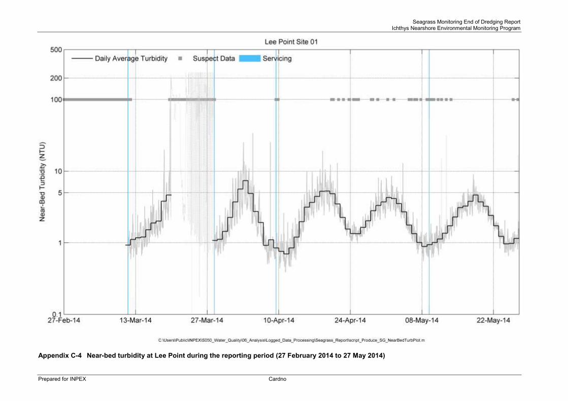
Seagrass Monitoring End of Dredging Report Ichthys Nearshore Environmental Monitoring Program
Prepared for INPEX Cardno
Appendix C-4 Near-bed turbidity at Lee Point during the reporting period (27 February 2014 to 27 May 2014)

Seagrass Monitoring End of Dredging Report Ichthys Nearshore Environmental Monitoring Program
Prepared for INPEX Cardno
Appendix C-5 Near-bed turbidity at Fannie Bay during the reporting period (27 February 2014 to 27 May 2014)

Seagrass Monitoring End of Dredging Report Ichthys Nearshore Environmental Monitoring Program
Prepared for INPEX Cardno
Appendix C-6 Near-bed turbidity at Woods Inlet during the reporting period (27 February 2014 to 27 May 2014)

Seagrass Monitoring End of Dredging Report Ichthys Nearshore Environmental Monitoring Program
Prepared for INPEX Cardno
Ichthys Nearshore Environmental Monitoring Program
APPENDIX D HISTORICAL CONDITIONS OF TURBIDITY
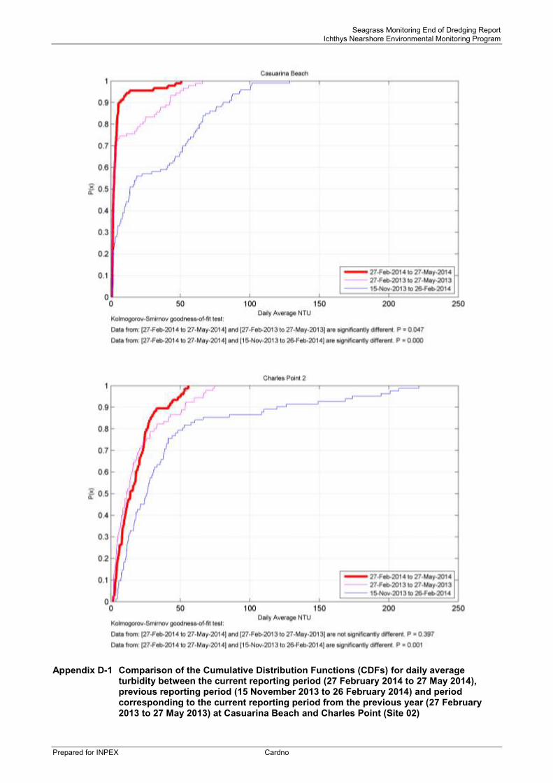
Seagrass Monitoring End of Dredging Report Ichthys Nearshore Environmental Monitoring Program
Prepared for INPEX Cardno
Appendix D-1 Comparison of the Cumulative Distribution Functions (CDFs) for daily average turbidity between the current reporting period (27 February 2014 to 27 May 2014), previous reporting period (15 November 2013 to 26 February 2014) and period corresponding to the current reporting period from the previous year (27 February 2013 to 27 May 2013) at Casuarina Beach and Charles Point (Site 02)

Seagrass Monitoring End of Dredging Report Ichthys Nearshore Environmental Monitoring Program
Prepared for INPEX Cardno
Appendix D-2 Comparison of the Cumulative Distribution Functions (CDFs) for daily average turbidity between the current reporting period (27 February 2014 to 27 May 2014), previous reporting period (15 November 2013 to 26 February 2014) and period corresponding to the current reporting period from the previous year (27 February 2013 to 27 May 2013) at East Point and Lee Point

Seagrass Monitoring End of Dredging Report Ichthys Nearshore Environmental Monitoring Program
Prepared for INPEX Cardno
Appendix D-3 Comparison of the Cumulative Distribution Functions (CDFs) for daily average turbidity between the current reporting period (27 February 2014 to 27 May 2014), previous reporting period (15 November 2013 to 26 February 2014) and period corresponding to the current reporting period from the previous year (27 February 2013 to 27 May 2013) at Fannie Bay

Seagrass Monitoring End of Dredging Report Ichthys Nearshore Environmental Monitoring Program
Prepared for INPEX Cardno
Appendix D-4 Comparison of the Cumulative Distribution Functions (CDFs) for daily average turbidity between the current reporting period (27 February 2014 to 27 May 2014), previous reporting period (15 November 2013 to 26 February 2014) and period corresponding to the current reporting period from the previous year (27 February 2013 to 27 May 2013) at Woods Inlet

Seagrass Monitoring End of Dredging Report Ichthys Nearshore Environmental Monitoring Program
Prepared for INPEX Cardno
Ichthys Nearshore Environmental Monitoring Program
APPENDIX E HISTORICAL CONDITIONS OF DAILY AVERAGE SIGNIFICANT WAVE HEIGHT

Seagrass Monitoring End of Dredging Report Ichthys Nearshore Environmental Monitoring Program
Prepared for INPEX Cardno
Appendix E-1 Comparison of the cumulative distribution functions (CDFs) for daily average significant wave heights between the current reporting period (27 February 2014 to 27 May 2014), previous reporting period (15 November 2013 to 26 February 2014) and period corresponding to the current reporting period from the previous year (27 February 2013 to 27 May 2013)