199

C-13

CHAPTER 4 SEAFLOOR CLASSIFICATION AND FEATURE DETECTION

1. INTRODUCTION 1.1 Hydrography includes the description of the features of the seas for a number of purposes not

restricted to navigation. The advent of sonar and swath echo sounders now enables a more complete and detailed description to the benefit of safer navigation and other uses. Obviously, it is impracticable to find every feature in every depth so the IHO have determined the minimum size of feature which should be searched for and measured in any particular area. Classification of the seafloor has been employed for minewarfare operations for many years but the advent of automated classification software has enabled wider usage, particularly in fishery and resource industries.

1.2 In this chapter, the phrases seafloor classification and seafloor characterisation, and feature

detection and object detection are synonymous 2. SEAFLOOR FEATURE DETECTION 2.1 Background 2.1.1 To ensure safe navigation it is necessary to detect features on the seafloor which may be a

hazard to navigation, whether natural or man made. A feature is defined as any item on the seafloor which is distinctly different from the surrounding area; it can be anything from an isolated rock on a flat sand seafloor to a wreck or obstruction. This activity is called seafloor feature detection. Feature detection can also be used to detect and identify features which are of interest to other seafarers, such as wellheads and mine-like features. The latter may not be of navigational significance but are, nonetheless, of importance to those concerned.

2.1.2 A traditional survey will develop the bathymetry of an area by running a regular series of

sounding lines throughout the area. Multibeam echo sounder (MBES) or side scan sonar (SSS) coverage is utilised for feature detection and to provide information regarding seafloor classification. In some instances the detection of features is more important than the acquisition of bathymetry. Specific features which have been identified on the MBES or SSS image will usually require a more positive check of its position and the least depth.

2.2 Standards 2.2.1 There are a number of feature detection standards the most relevant being those contained in

IHO S-44 and IHO S-57. 2.2.2 IHO S-44 - Minimum Standards for Hydrographic Surveys 2.2.1.1 S-44 Table 1, summarised at Tables 4.1 and 4.2 below, specifies where a feature search is to be

undertaken and system detection capabilities for each Order of survey: 2.2.1.2 Once detected any features considered significant should have its position and the least depth

over it determined to the standards detailed in S-44 Table 1.

200

C-13

IHO S-44 Order and example areas Search Requirement

Special Order Areas where under-keel clearance is critical. Full sea floor search required.

Order 1a Areas shallower than 100 metres where under-keel clearance is less critical but features of concern to surface shipping may exist.

Full sea floor search required.

Order 1b

Areas shallower than 100 metres where under-keel clearance is not considered to be an issue for the type of surface shipping expected to transit the area.

Full sea floor search not required.

Order 2 Areas generally deeper than 100 metres where a general description of the sea floor is considered adequate.

Full sea floor search not required.

Table 4.1 “IHO S-44 Search Requirements”

IHO S-44 Order System Detection Capabilities

Special Order Cubic features >1.0 m

Order 1a Cubic features >2.0 m in depths up to 40 m or 10% of depth beyond 40 m

Order 1b Not applicable.

Order 2 Not applicable.

Table 4.2 IHO S-44 System Detection Capabilities 2.2.3 IHO S-57 - Transfer Standards for Digital Hydrographic Data 2.2.3.1 S-57 specifies "Zones of Confidence" (ZOC) as the method of encoding data quality

information. ZOC were adopted to provide a simple and logical means of classifying all bathymetric data and displaying to the mariner the confidence the national charting authority places in it. Areas are classified by identifying various levels of confidence that can be placed in underlying data using a combination of depth and position accuracy, thoroughness of seafloor search and conformance to an approved quality plan.

2.2.3.2 ZOC A1, A2 and B are generated from modern and future surveys with, significantly, ZOC A1

and A2 requiring a full seafloor search, i.e. full feature detection. ZOC C and D reflect low accuracy and poor quality data, whilst ZOC U represents data which is unassessed, but not unsurveyed, at the time of publication. ZOC are designed to be depicted on paper charts, as an insert diagram in place of the current reliability diagram, and on electronic displays.

2.2.3.3 It must be emphasised that ZOC are a charting standard and are not intended to be used for

specifying standards for hydrographic surveys or for management of data quality by individual hydrographic authorities. Depth and position accuracy specified for each ZOC refer to errors of final depicted soundings and include not only survey errors but other errors introduced in the chart production process.

201

C-13

2.2.3.4 S-57 ZOC Feature Detection criteria are at Table 4.3:

S-57 ZOC Search Requirement

ZOC A1 full area search undertaken, all significant seafloor features detected and have had their depths measured. (see Note) ZOC A2

ZOC B full area search not achieved, uncharted features hazardous to navigation may exist.

ZOC C full area search not achieved, depth anomalies may be expected.

ZOC D full area search not achieved, large depth anomalies may be expected.

ZOC U quality of bathymetric data yet to be assessed.

Table 4.3 ZOC Feature Detection Criteria Note: Significant seafloor features are defined in S-57 as those rising above depicted depths

by more than: 0.1 x depth, in depths <10 m, 1.0 m in depths of 10-30 m and (0.1 x depth) minus 2.0 m in depths >30 m. 2.2.3.5 S-57 also details the relevant position and depth accuracy required of measured features. 2.2.4 Detection of Hazardous Features 2.2.4.1 The surveyor must remain cognisant of the fact that many features which are potentially

hazardous to navigation do not fit the S-44 “cubic feature” criteria; for example the masts of wrecks and wellheads. However, ZOC criteria do take such features into account if they rise above depicted depths by the prescribed amount. The ability to detect such features is a critical issue when considering the type of system to be used to undertake feature detection. For instance, these types of features will normally be detected by SSS but may not be detected by MBES, lidar and other such systems due, for example, to the beam footprint or “filtering” algorithms.

2.2.4.2 As far as the surveyor is concerned the purpose of a sonar sweep is to ensonify the area

between adjacent lines of soundings in order to detect any feature of significance to the mariner. Although no hard and fast definition of the minimum length of a wreck can be given, features less than three metres in length are unlikely to be sufficiently proud of the seafloor to cause concern. There will of course be occasions when this is not so (e.g in coral areas or when searching for masts) and the Surveyor must examine all sources of data available to him before deciding on the minimum length feature he wishes to detect.

2.2.4.3 Note that in all calculations that follow, involving speeds over the ground that must not be

exceeded, the feature length is used and no account is taken of feature height. What is used for calculations is the maximum length of feature that just fails to receive five ‘pings’, this being

202

C-13

considered the minimum to achieve feature detection. How much of the energy in the five pings on the feature that returns to the transducer is dependent upon:

feature shape, extent, composition and aspect, sonar conditions and nature of the seafloor and other factors. 2.2.4.4 The amount of energy returned from the feature will control the intensity of the printed mark. 2.2.5 Military Requirements 2.2.5.1 Military forces often require detection of features smaller or deeper than those required for the

safety of navigation, for example some strive to detect features with a volumetric size of 0.5 m on the continental shelf in depths to 200 m. Minewarfare forces, using specialised sensors, aim to detect and classify even smaller features. Whilst these reflect particular capabilities not normally required of the surveyor employed in nautical charting, there is a resultant effect on the development of systems capable of achieving them becoming available on the commercial market.

2.2.6 Reporting Features 2.2.6.1 Whilst it is desirable to investigate every feature which meets the above criteria in complex

areas this will not be possible. Surveyors may need to use their own judgement as to which features warrant investigation after considering the available resources, the likely use of the area (draught of vessels etc.) and the likely significance of the feature noting the general depths in the area. For example, a shoal of 26 m in general depths of 28 m may not warrant further investigation if the draught of vessels using the area is only 12 m. This will particularly be the case if a ship transiting the area must at some point pass through general depths of, say, 20 m. In such cases it may only be necessary to ensure that there is no indication of much shoaler water (e.g. by interlining, sonar etc.).

2.2.6.2 The above criteria should also be used to ascertain whether or not a feature should be included

in any Report of Survey. In complex areas this list can become unwieldy; therefore the Report need only include those features which are truly significant in terms of general depths and likely usage.

2.2.6.3 At the end of each survey the surveyor, being the only person with all the facts at his disposal,

must give a firm opinion as to the status of each feature located, i.e. wreck, sea floor type, unexamined etc., with findings included in their Report. Newly discovered features, which may be dangerous to surface or submarine navigation, and charted features, which are found to be significantly changed, are to be reported to the responsible National Hydrographic Office (NHO) immediately. Uncharted features in depths less than 750 m would normally be considered for Notice to Mariners action.

2.3 Methods of Feature Detection 2.3.1 Overview 2.3.1.1 There are a number of methods with which to achieve feature detection. SSS has a well proven

203

C-13

feature detection capability and can still be considered the most reliable means. However, SSS is subject to operational limitations in that it is generally towed behind the survey vessel, which introduces positional errors for features. These errors can be reduced by use of transponders in the towfish and/or running past the feature in the opposite direction to obtain an average position. SSS operations are also subject to the nadir gap which requires lines to be run with sufficient overlap to detect features under adjacent tracks.

2.3.1.2 One of the main limitations of SSS is the speed of advance required to achieve sufficient pings

on a particular feature. With few exceptions this limits SSS operations to about six knots, which impacts rate of effort. The advent of MBES offers the chance of meeting feature detection requirements at higher speeds and therefore increased rate of effort. To date, however, MBES detection of features of the size that meet IHO Special Order and ZOC A1/A2 requirements or other small and potentially hazardous features, cannot be guaranteed unless certain precautions are taken, such as limiting the useable swath width and calculating an appropriate speed of advance for ‘ping’ rate.

2.3.1.2.1 The geometry of a SSS transducer in relation to a feature is the key factor which makes it such

a successful tool for feature detection. The shadows cast behind a feature, proud of the seafloor, are the telltale sign that a feature has been ensonified. The geometry of the MBES transducer in relation to seafloor features results in the loss of almost all shadow-casting capability. A surveyor wishing to use MBES for feature detection must then rely on the MBES’s other characteristics in order to look for any features. These characteristics are high resolution bathymetry and amplitude backscatter coupled with a positioning capability allowing for very accurate repeatability. In addition, whilst features are normally capable of being detected by an operator during SSS data acquisition, detection using MBES is far more uncertain at this stage and post processing is usually required to allow results to be seen.

2.3.1.3 Other sensors which can be used for feature detection include singlebeam echosounder (SBES),

forward looking sonar, magnetometer and remote methods such as Airborne LiDAR Bathymetry (ALB) and Airborne Electromagnetic Bathymetry (AEMB). Mechanical feature detection methods, less used these days, include wire sweep, drag and diver.

2.3.2 Side Scan Sonar 2.3.2.1 Dual-channel SSS is now accepted as an essential aid to modern surveying and it remains the

case that no survey on the continental shelf can be considered complete unless a comprehensive sonar sweep has been carried out and all contacts investigated.

2.3.2.2 In addition to locating wrecks and obstructions between survey lines, SSS also provides a

considerable amount of other seafloor information. These data, when combined with seafloor samples and depth contours to produce seafloor classification, are of great value to those involved with amphibious, minewarfare and submarine operations. The importance of this information has grown over the years to such an extent that, in many surveys, sonar rather than bathymetric considerations govern the selection of line direction and spacing. However, great care is needed in the preparation and checking of these data if their full potential is to be realised.

204

C-13

2.3.2.3 When used in hydrographic surveying, SSS has four main functions: • The detection of wrecks and obstructions between sounding lines. Although precise position

and least depth cannot be determined by SSS, a properly tuned and operated sonar will detect nearly all significant features between lines.

• The detection of other seafloor features. Correctly used, SSS can detect very small seafloor

features. Whilst not hazardous to navigation the positions of such features, or groups of features, are of considerable importance in both submarine and minewarfare operations.

• The gathering of seafloor classification data. Knowledge of the texture of the seafloor,

combined with samples, is of great importance for submarine bottoming and minewarfare operations, and for fisheries and resource development.

• The identification of mobile areas of seafloor. The presence of sand-waves and ripples are

indications that the seafloor in a particular area is mobile. On major shipping routes such areas may require periodic re-survey to ensure safety of navigation.

2.3.3 Theoretical Considerations 2.3.3.1 The strength of the signal returned by a given feature is governed by several factors linked by

an expression known as the “sonar equation” which may be used to determine whether a particular type of feature will or will not be detected. A good explanation of the terms involved in this equation is given in the 1981 FIG/IHO “Report on the Detection of Depth Anomalies”. The standard textbook that should be consulted if a further study of this subject is required is “Principles of Underwater Sound” by R.J. Urick. It must be stressed that this equation can form only the starting point for a consideration of SSS performance because it is not possible to know all the equation terms.

2.3.3.2 Short range coverage. There is a region close to the towfish where gaps in the sonar cover may

occur. These gaps need to be considered in two planes (see Figure 4.1): Direction of Tow

Fig. 4.1 SSS Horizontal and Vertical Beam Coverage

205

C-13

• The vertical plane. The main beam of the sonar has a width in the vertical plane of about 50°, with the beam axis tilted 10° downwards. There is, therefore, a region under the towfish which lies outside the main beam; the size of this region is governed by the height of the transducers off the seafloor. The original concept of this area not being ensonified at all is incorrect. Unless the towfish is a long way off the seafloor this zone is covered by side lobes from the transducers, and parts will receive some sound energy from the fringes of the main beam. (The “edge” of a beam is usually taken as the half-power line, but this is not an absolute cut-off point and some energy exists outside it). Whilst a gap in the record under the towfish does occur, it is considerably smaller than originally thought and may only be a few metres in extent. Nevertheless, this gap must be covered by sonar from the adjacent lines.

• The horizontal plane. There is an area close to the towfish (the “near field”) where the sound

pulses have parallel edges. As a result, gaps may occur between individual pulses of sound. The gap between pulses in the near field is a function of ship speed and pulse repetition rate. Beyond this area, the spreading of the beams closes the gaps to give total coverage. Small contacts are therefore likely to be missed close to the towfish rather than further away from it.

2.3.3.3 Planning Area Searches. Two different methods of planning area searches can be used: • Detecting contacts close to the towfish. The search is planned so that the smallest required

contact can be detected close to the towfish. The limiting case requires such contacts in the near-field of the sonar beam to receive five pulses; outside this area, beam expansion ensures they will receive at least five pulses.

• Detecting contacts further away from towfish. The zone where small contacts may not be

detected can be calculated for a given range scale in use and speed over the ground. Line spacing can then be adjusted so that sweeps from adjacent lines at least cover the gap. Alternatively, line spacing can be fixed and speed adjusted to ensure that full coverage is achieved. Thus with a range scale of 150 m in use and at a speed at which small contacts may not be detected within the first 25 m, line spacing must not be more than 125 m.

2.3.3.4 The second of the above methods is usually employed on area searches as it allows a faster

speed of advance. For a line-spacing of 125 m using the 150 m range-scale, one metre contacts will be detected in the near field at a speed of 3.6 knots. Relying on detecting them from adjacent lines allows a speed increase to 7.0 kt. Details of the calculation follow (see ‘Feature Detection’ and ‘Calculation of Speed of Advance’).

2.3.3.5 Confirming SSS Performance. Whilst these calculations will provide theoretical capabilities it

is essential that a SSS’s performance is confirmed in the field prior to use. This is achieved by selecting a suitable feature, reflecting the type and size of feature required to be detected during the survey, and towing the SSS past it. Both sonar channels, i.e. both sides, and each range scale should be tested to determine the maximum detection range.

2.3.3.6 Position of the Sidescan Towfish. Towing the sonar transducers astern of the vessel has several

advantages including removing the sensor from the effects of vessel motion and operating it at a height above the seafloor which will enable the optimum shadow. However, there is a disadvantage in that it also introduces uncertainty as to the position of the towfish. This error has three components:

206

C-13

• an along-track component, caused by uncertainty in how far the towfish is astern of the vessel; this depends on the length of cable out, depth of towfish and vertical catenary of the cable (the last two also vary with the ship’s speed);

• an across-track component, caused by deflection of the towfish by tidal stream or current,

and by ship manoeuvres; • errors in the position of the ship or boat, which will be transferred to the towfish. 2.3.3.7 Towfish position can be determined using an Ultra Short Baseline (USBL) positioning system

which requires transducers/receivers to be fitted in the vessel and towfish; however the accuracy of this system deteriorates rapidly depending on the length of tow. An alternative method, under development in Australia, utilises the direction and angle of depression of the tow cable over the stern of the vessel, together with a model of the catenary of the tow cable to predict, reasonably accurately, the towfish position.

2.3.3.8 In addition, the attitude of the towfish may vary both longitudinally and about its axis and thus

the direction of the transducer beams may fluctuate. This is especially true if the ship's course or speed are frequently changing and emphasises the need for generous overlaps during sonar sweeping. Planning to theoretical limits of performance is almost certain to lead to gaps in the sweep in reality.

2.3.3.9 Hull Mounting. SSS can be mounted in the hull of a surface vessel. The advantages of this are

that its position, and hence orientation, are accurately known and therefore the positioning of detected features is relatively easy. Hull mounting also enables freedom of manoeuvre for the vessel which is no longer required to tow the sensor. However there are a number of disadvantages to hull mounting including the effect of vessel motion on SSS ensonification and performance, possible mutual interference with other hull mounted sensors, e.g. MBES, and the fact that it is unlikely that the SSS will be operated at the optimum height above the sea floor. Hull mounting is often the best method when operating in shallow water or in areas where the seafloor topography is potential hazardous, e.g. reef strewn. Otherwise, the disadvantages of hull mounting would normally outweigh the advantages.

2.3.4 Operational Constraints 2.3.4.1 Hydrodynamic Stability of the Towfish. Under most conditions the towfish is largely

decoupled from the effects of ship's motion by the flexibility of the tow-cable. The assumption is usually made that the towfish is completely stable in roll, pitch and yaw, although some motion in all these planes undoubtedly occurs. Roll probably has relatively little effect on the sonar picture, being compensated for by the wide beam angle in the vertical plane. A permanent list in one direction, which may be caused by a distorted fin or a twist in the cable can, however, markedly decrease performance. This should be suspected if one channel gives a different quality of picture to the other.

2.3.4.2 In extreme cases it may be necessary to rely only on the “good” channel and allow for this in

planning survey lines. Pitch and yaw are more significant; with such a narrow beam-width in the horizontal plane, these motions could decrease detection probabilities of small features. A feature that would receive at least five pulses with a stable towfish may only receive three or four if the towfish is oscillating in either of these directions.

207

C-13

2.3.4.3 The problem of towfish stability is believed to be less important than that of towfish position. In rough weather the effects of towfish oscillation can usually be clearly seen on the trace. Under these conditions the reduction in the probability of detecting small features must be considered. With the increasing use of heave compensators and motion sensors for echo sounders and the greater importance attached to detecting small contacts, sonar conditions rather than echo sounder performance may be the limiting factor for effective surveying.

2.3.4.4 Height of Towfish. For most work the optimum height of the towfish above the seafloor is

10% of the range-scale in use, i.e. on the 150 m scale the towfish should be 15 m above the seafloor. SSS transducers are directed slightly downwards so flying the towfish too close to the seafloor may reduce the range from which returns can be received. If the towfish is too high acoustic shadows may not be formed behind obstructions making them more difficult to detect. This is especially true in deep water when a compromise has to be made between the need for getting the towfish down to a useful depth and maintaining a reasonable speed of advance.

2.3.4.5 In areas of very high seafloor relief it may be prudent to tow the sonar higher than normal; in

this event the reduction in acoustic shadow on features standing proud of the seafloor must be borne in mind. This effect is worst close in to the towfish where detection of small contacts is already at its most difficult.

2.3.4.6 In shallow water it may not be possible to get the towfish as high off the seafloor as desirable.

Although the recorder will be giving a background trace across the entire width of the paper, the sonar beam may not be ensonifying the entire range. Under these conditions the only solution is to reduce both the range scale and the line spacing.

2.3.4.7 As a further limitation in shallow water the transducers may be very close to the surface with

little tow-cable streamed. This will introduce the problem of surface noise (such as waves and ships wake) degrading performance and may also lead to the towfish being adversely affected by the motion of the ship. The effects of water layers and thermoclines on SSS can usually be ignored, they have very little effect on the range at the frequencies used.

2.3.4.8 When investigating contacts with sonar the towfish should always be sufficiently high above

the seafloor to allow it to pass over the obstruction in the event of an accidental “on top”. The least depth over a feature can usually be estimated initially from the shadow length obtained during the area search.

2.3.4.9 If it becomes necessary to tow the towfish at a height other than the optimum, a confidence

check should always be carried out to confirm the system continues to meet detection and other requirements. Towfish height can easily be controlled by a combination of wire out and ship’s speed. Quickly heaving in a length of cable will “snatch” the towfish upwards rapidly, after which it will settle back down more slowly. This technique can be very useful in lifting the towfish over unexpected dangers. As the length of wire streamed increases this method becomes less effective.

2.3.4.10 Depressors. Some SSS towfish can be equipped with depressors which will drive the fish

deeper for any given length of tow cable or speed of advance. Whilst this can reduce the length of tow required there are a number of disadvantages to using depressors:

• they increase strain on the cable resulting in the requirement for a more powerful winch if

scope is to be adjusted underway; and manual operations can become impracticable;

208

C-13

• the shorter scope of cable results in the transmission of ship movement down to the towfish; • they can reduce the effect of an increase in speed and/or reduction in scope of tow cable on

the towfish height, thus negating the use of this technique to overcome unexpected dangers. 2.3.4.11 When operating in close proximity to the sea floor it is prudent to ensure the towfish is fitted

with a trip mechanism that enables it to flip over and still be retrieved after a strike. In this case it is possible the fins will be lost, but at least the towfish itself is recovered. Some modern SSS avoid the problem of fin loss by only having upward facing fins.

2.3.4.12 Direction of tow. In normal circumstances SSS should be towed into and out-of the

predominant tidal stream/current in order to minimise their effect on the towfish in the form of across track positional errors. Where tidal stream/current effects are not an issue the SSS should be towed parallel to the bathymetric contours. This minimises the requirement to have to continually adjust the scope of tow when steaming into and out-of shallow water.

2.3.4.13 However, there are exceptions to these rules. In sandwave areas, in particular, it may be

necessary to tow the SSS at right angles to the axis of the sandwaves. This ensures that the SSS looks along the sandwave crests/troughs to avoid the possibility of shadow areas where features will not be detected, see Figure 4.2.

Fig. 4.2 Sidescan Sonar – Potential Shadow Areas in Sandwaves and Correct Direction of Tow”

2.3.4.14 Effective Sonar Range. The presence of marks on the sonar trace does not necessarily indicate

that returning echoes are being received. Transmission losses, interference from other sources of noise, water conditions and recorder limitations all restrict the useful range of SSS. For example with a 100kHz sonar, a maximum range of 270 m is about all that can be expected for even large wrecks, with small contacts (1-2 m) unlikely to be detected beyond about 120-150 m. Detection range varies between different SSS models and frequencies - the higher the frequency the less the detection range, although the resulting picture may be better. The best results will usually be achieved by restricting the range scale to 150 m to take advantage of the higher pulse rates and greater definition. A short test using a suitable seafloor contact at varying ranges will usually provide information on sonar conditions in the survey area.

2.3.5 Distortions of Sonar Records 2.3.5.1 Sonographs never represent isometric maps of the seafloor. Various distorting factors have to

towfish shadow area

correct direction of tow ax

is o

f sa

ndw

aves

sandwave – crest / trough

209

C-13

be recognised when interpreting sonograph mosaics in map form, unless the distortions have been eliminated digitally before the mosaic has been compiled. The main causes of distortion are:

• compression of sonograph picture with speed increase - a distortion will occur parallel to the

course made good due to variable ship speeds and constant paper feed speed, resulting usually in a compression of the record in this direction;

• the height of the towfish above the seafloor will introduce a lateral distortion perpendicular

to the direction of travel; • a sloping seafloor will introduce distortions perpendicular to the direction of travel which are

different on the up-slope and down-slope sides. 2.3.5.2 For a given ship’s speed, range scale, paper speed and towfish height, the distortions can be

calculated. During area sweeps these effects generally only need to be considered when plotting contacts; during investigations they need to be considered in detail. Speed during investigations should be adjusted to give as little distortion as possible, about 3.0 kt is usually ideal.

2.3.5.3 Lloyd Mirror Effect. During sonar operations in very calm conditions reflection of some of the

sonar energy can occur from the sea-surface, as shown in Figure 4.3. This is known as the Lloyd Mirror Effect and results in a series of maxima and minima in the sonar image. This effect normally occurs only when the towfish is close to the surface and can be minimised by towing the towfish deeper.

Fig. 4.3 Lloyd Mirror Effect 2.3.5.4 Cross Talk. Cross talk between two SSS channels can result in a mirror image of sea floor

features from one channel being displayed on the opposite channel, albeit usually fainter. Cross talk can result in the true image on the effected side being obscured. This may prevent detection of features or to the erroneous ‘detection’ of what are, in effect, copies of real features from the opposite side. This can be a particular problem in areas where there are numerous features in which case it can be difficult to verify what is real and what is not.

210

C-13

2.3.5.5 Tilt Effect. If the side scan towfish is not being towed level, in other words it is tilted to one side, the channel that is facing downwards towards the sea floor will result in a stronger return signal and therefore a darker image; on the other hand the channel that is facing upwards will result in a lighter image. Seafloor classification is based on interpreting the image shading, a result of the relative strength of the return signal from different seafloor types. The tilt effect can therefore result in difficult or even erroneous interpretation.

2.3.5.6 Automatic Gain Control (AGC). AGC was introduced as a means of ensuring the SSS image

was optimised for feature detection. In other words in areas of strong return, such as rock, the gain was automatically decreased to enable features to be detected against a ‘light’ background. However, as with the tilt effect, altering the gain and hence the resulting image shading, also renders seafloor classification difficult, if not impossible. For this reason AGC should be turned off if the sonar image is to be used for seafloor classification.

2.3.5.7 Wash and Wake. If the SSS is towed too close to the surface the image can be affected by

returns from the wash or wake of other vessels or even the towing vessel itself if it has recently made a turn. Again, such interference can seriously impact seafloor classification and it is important that a sonar log is maintained so that such incidents can be recorded to assist subsequent image interpretation.

2.3.5.8 Thermocline. As with any sonar, SSS transmissions are subject to the effects of their passing

through water with changing properties and which may result in distortion of the image. Whilst software can be used to ‘mould’ the image back into shape, it is the important for the surveyor to know, and hence the degree of sonar ensonification which is used to overcome this problem. For instance, in areas significant to navigation, a higher level of ensonification redundancy may be required with adjacent lines run in opposite direction and possibly additional lines at right angles, with a short range scale selected. In less important areas the range scale employed may be greater and the degree of overlap and redundancy less and therefore distortion can become more of a problem.

2.3.5.9 “Sound Underwater Images - A Guide to the Generation and Interpretation of Side Scan Sonar

Data” (Fish JP & Carr HA, 1990) is an example of a reference text that may be used to assist sonar interpretation.

2.3.6 Feature Detection 2.3.6.1 The following assumptions are made: • feature size is defined as the length presented normal to the sonar beam; • the minimum number of returns to make a discernible mark on the trace is taken as five; • sound velocity is assumed to be 1500 m/sec; • beam angle of the sonar is 1.5°.

211

C-13

2.3.6.2 Terms and Units: pulse interval - t seconds

pulse repetition interval - F pulses per second

ship's speed (over ground) - V metres per second

feature length - L metres

velocity of sound in seawater - C metres per second

recorder range scale - Rm metres

beam width - Bw metres

slant range to contact - Rs metres

length of array - l metres

distance travelled between pulses - d metres 2.3.6.3 Basic Equations: F = C pulses per second; or, t = 1 seconds 2Rm F Because φ is a very small angle, beam width at a given range (Bw) = Rs x φ 2.3.6.4 It can be seen from Figure 4.4 that Feature A is the largest feature that CANNOT receive five

pings; it can receive a maximum of four (i.e. pings 2, 3 and 4 and either ping 1 or 5). However, theoretically, a small increase in Feature A's length would mean that it received five pings; in general, for N pulses its length is given by:

L = V x t x (N - 1) – Bw (4.1)

2.3.6.5 Feature B is the smallest feature that MUST (theoretically) receive five pings; it is caught by

the first and just missed by the sixth. Its length is given by:

L =V x t x N - Bw (4.2) Essentially this is the same equation as used to determine speed whilst echo sounding. Both

formulae assume that the sonar beam is divergent. 2.3.6.6 In general, equation (4.1) is used when determining either: • the length of feature that will receive five pings at a given speed over the ground; • the speed over the ground that cannot be exceeded if a feature of a given length is to receive

five pings. 2.3.6.7 There may be occasions when the surveyor feels it more prudent to use equation (4.2) giving a

greater probability of detection.

212

C-13

Fig. 4.4 Diagram showing Feature Detection 2.3.7 Calculation of Speed of Advance (SoA) 2.3.7.1 A typical survey scale is 1:25,000 in which case the usual spacing of lines is 125 m with the

SSS on the 150 m range scale. In general, it is advantageous if bathymetry and sonar sweeping can be carried out at the same time. With lines 125 m apart a swathe 25 m either side of adjacent lines is ensonified, although this may be reduced with wayward line-keeping.

2.3.7.2 To recognise a feature on the SSS trace it is necessary to ensure it receives five pings. To

identify it as a significant feature requires a confirmatory detection from another line. This does not mean that contacts not detected on adjacent lines may be discarded as spurious but that a small wreck at the outer edge of the SSS trace may easily be overlooked.

2.3.7.3 In an area sweep it is then necessary to determine the speed over the ground which must not be

exceeded in order that a feature of one metre in length should receive five pings from two adjacent lines. This gives the Speed over the Ground (SoG) which should not be exceeded.

Fig. 4.5 Calculating Speed of Advance

213

C-13

2.3.7.4 In Figure 4.5 A, B and C are three lines spaced 125 m apart. A survey vessel is operating its SSS on the 150 m range scale. What criteria must be satisfied?

2.3.7.5 Near Field. The near field limit is usually within 20 m. Therefore with a 25 m overlap from

adjacent lines a feature which would not have received five pings at a given range in the near field on line B will get five pings from both lines A and C. In this case the near field detection speed of 3.6 knots is not a limiting factor.

2.3.7.6 Far Field. Contact 1 should be detected from lines A and B, Contact 2 will get five pings from

lines A and C, Contact 3 from lines B and C. It is necessary to calculate the speed over the ground that must not be exceeded if a contact of length L m is to get five pings at 25 m.

If L = 3.0 m then: From equation (4.1) the maximum length of feature that will not get five pings is:

L = V x t x (N - 1) – Bw where Bw = 25.0 ·x φ

N = 5

t = 0.2 sec

L = 2.999 m (see Note) Note: because theoretically a slightly longer feature, i.e. 3.0 m, should get five pings. rearranging: V = L + Bw (N - 1) x t = 2.999 + 0.6545 4 x (0.2) = 4.57 m/sec or 8.9 kt 2.3.7.7 In fact for practical reasons the towfish should not be towed at speeds over the ground in excess

of 8.0 kt, or small features will be missed, or 10 knots through the water since above this speed the towfish is liable to yaw. Note also that if five pings to a feature are to be “guaranteed” then equation (4.2) should be used giving a V of 3.65 m/sec or 7.1 kt.

2.3.7.8 If the requirement is to detect features 1.0 m in length from two lines then: V = 0.999 + 0.6545 4 x (0.2) = 2.067 m/sec or 4.0 kt

214

C-13

2.3.7.9 However if five pings into a one metre feature from one line only are to be required then: V = 0.999 + (72.5 x Bw) 4 x (0.2) = 3.623 m/sec or 7.0 kt 2.3.7.10 The danger with using the last of the above equations is that the probability of detection of a

small feature in a “one chance only” situation is low. 2.3.7.11 “Fast” SSS. As technology evolves some SSS are able to be operated at faster speeds over the

ground than was previously possible. An example is the Klein 5000 series, which employs beam steering and focussing techniques simultaneously generating several adjacent, parallel beams per side. This “multibeam” design permits higher towing speeds whilst providing high resolution imagery. Other SSS developments include the use of interferometric, multi-pulse and synthetic aperture techniques. However, as with all such sensors, it is essential that its performance is validated against known targets, which represent features required to be detected. Validation should be followed up by initial and regular repeat confidence checks in the survey area.

2.3.8 Track-Keeping Errors 2.3.8.1 A question that needs to be addressed is how far off track can the survey vessel go before a gap

in coverage is created? Assuming only one detection (five pings) is required to a 1.0 m feature, a standard 1:25,000 survey is being undertaken with lines 125 m apart and range scale 0-150 m selected, then overlap is 25 m. The sum of any errors must be contained within this figure. For example:

towfish position e1 10 m

vessel navigation e2 5 m

slope effect e3 1 m

sound velocity variations e4 1.5 m

therefore ∑e2 = 128.25 m

total error RMS E = 11.3 m 2.3.8.2 Overlap is 25 m, however only 24 m is useable (the contact has to paint) therefore total

allowable track error = √ [242 - Σe2] = 21 m 2.3.8.3 This assumes that a feature is detectable at 149 m where it will paint as a black dot 0.8 mm by

0.8 mm with a 1 mm shadow (that is if the shadow is not obliterated by the 150 m range line). A more prudent off track allowance would be 15 m; this plots as 0.6 mm at a scale of 1:25,000.

2.3.9 Practical use of Side Scan Sonar 2.3.9.1 Area Sweep is the name given to the standard hydrographic sonar search method. The

categories of sonar sweep required for any given survey will be specified in the survey instructions. An example of categories of SSS search is as follows:

215

C-13

Category A and B. Search in one direction and/or its reciprocal using SSS. Where practicable, adjacent lines are to be run in opposite directions. Searches for all listed wrecks are to be conducted. Examples of sonar line spacing, range scale, overlap to be achieved and maximum speed over the ground to be used are given at Table 4.4.

Category A sweeps are intended to be the standard sweeps for coastal and inshore areas not

subject to routine re-survey. These sweeps are designed to achieve a theoretical seafloor ensonification of 240%, i.e. [2 x effective sonar range/line spacing] x 100 = % ensonification.

Category B sweeps achieve a theoretical seafloor ensonification of 133% and may be used for

routine re-surveys and in depths greater than 100 m where detection of all features is less critical.

Category C. Only searches for listed wrecks are to be conducted. Category D. Special searches as ordered. This includes special instructions for use of

particular SSS and hull mounted sonars etc.

Category Type of Survey Sonar Line

Spacing Sonar Range

Scale

Max Speed over the

Ground

Adjacent Line Overlap1

A1 Special 125 m 150 m 6 kt 25 m

A2

inshore & coastal surveys at >1:25,000 in depths <15 m

62.5 m 75 m

8 kt

(See Note 2)

12.5 m

inshore & coastal surveys at >1:25,000 in depths <50 m

125 m 150 m 25 m

shelf surveys in depths >50 m and/or scale <1:25,000

250 m 300 m 50 m

B1 routine re-surveys 250 m 150 m 50 m

B2 shelf survey scale < 1:25,000 in depths >100 m

500 m 300 m 100 m

Table 4.4 – Sidescan Sonar Search - Categories A and B - Example Criteria

Notes:

1. The overlap under adjacent lines is to allow for limited wayward line-keeping and positional inaccuracies. If the surveyor considers positional inaccuracies and/or wayward line-keeping exceed this figure then he should adjust the line spacing or range scale, with subsequent speed adjustments, as necessary.

216

C-13

2. See previous comments with regard to use of “fast” SSS which may enable these speeds to be increased.

2.3.9.2 It is emphasised that these reflect minimum standards; if in doubt over sonar performance, line

spacing should be tightened or speed reduced. In all cases it is necessary to refer to the relevant IHO S-44 or S-57 ZOC standards to ensure search requirements are met.

2.3.9.3 The use of a regular series of parallel straight lines remains the most efficient way of covering a

survey area. The line direction will be close to the direction of the tidal stream to minimise towfish offset. The line spacing for the sonar lines is determined by the range scale in use and the overlap required. It is recommended that the overlap between adjacent swaths is 125%.

2.3.9.4 For military surveys on the continental shelf in water depths less than 200 m, the requirement is

often to detect all contacts larger than one metre in extent. With existing equipment this cannot easily be achieved and a compromise between the requirements of sonar and bathymetry must be reached. A sonar sweep which will detect one metre contacts in depths less than 140 m provides this compromise. For the normal scale of l:25,000, this means a line spacing of 125 m, sonar range scale of 150 m and a speed over the ground no faster than 7 knots. Existing equipment cannot effectively be deployed deeper than 150 m and, in water between 150 and 200 m depth, the search will be restricted to locating large wrecks and obstructions.

2.3.9.5 Unmanned Underwater Vehicles (UUV). The employment of UUV equipped with SSS and

MBES is becoming increasingly common. These platforms enable sensors to be operated at great depth and at the appropriate altitude above the seafloor. Thus it is likely that small features will be capable of detection at greater depths than is currently possible when employing surface vessel mounted or towed sensors.

2.3.9.6 Sonar sweeps should always be undertaken with lines orientated as closely as possible parallel

to the main tidal flow in the survey area. The cross-track errors in the position of the towfish are invariably greater than those along the track and every effort should be made to minimise them. At a speed of 6 kt with 400 m of wire out and a tidal stream of 2 kt, a difference of 10° between tidal flow and line direction can offset the towfish 17 m from the line.

2.3.9.7 The running of an extra sonar line immediately outside each edge of the survey area is

necessary to ensure that the ordered category of sweep continues to the limit of the area. Similarly, care must be taken to ensure that the SSS towfish has cleared the edge of the survey area before a survey line is ended.

2.3.9.8 It must be remembered that speed and feature detection probabilities calculated here are

theoretical and take no account of adverse sonar conditions and equipment failings. 2.3.9.9 Plotting of Contacts. The detection of seafloor contacts between survey lines is one of the main

reasons for using SSS. The ultimate use of the information must always be considered when deciding which contacts to plot; for example, submarines will not take the ground in areas of rough seafloor and minewarfare operations will usually be selected to avoid them. In areas of smooth seafloor the aim must always be to detect and plot every contact; in more rugged areas this standard will have to be relaxed. All such contacts must be plotted and allocated a contact number which will ultimately be included in the seafloor classification model.

217

C-13

2.3.9.10 Various techniques have been developed to plot contacts from manuscript SSS records; all attempt to reduce the errors in the contact position caused by errors in towfish position and orientation. Different techniques are to be used for contacts plotted from area searches, investigations and examinations:

• Contacts from area searches are usually plotted from two directions 180° apart. The standard “layback and offset” method should be used, with the mean of the two positions adopted as the most likely position.

• Investigations should produce a minimum of two pairs of passes for each contact at right-

angles to each other, orientated in such a way as to fix the extremities. • When a contact is examined by echosounder, the best “on top” position is to be used in

preference to any SSS derived one, where possible an echo sounder line should pass the length of the long axis of the contact.

2.3.9.11 Measurements by Sonar. A good “beam-on” SSS picture of a wreck or obstruction can usually

be used to estimate its height above the seafloor using the sonar “shadow”. Although not accurate enough for charting purposes, this height is very useful for the safety of both ship and towfish when planning investigations. Estimates of the beam and length of a wreck can also be obtained from the sonar trace. The following points should always be considered:

• when estimating heights from sonar shadows the presence of higher parts of the wreck (such

as masts), which do not throw a detectable shadow, should always be borne in mind; • shadow heights must be measured from both sides of the wreck and the results meaned - this

helps to correct for errors introduced by seafloor slope (it should be noted that heights obtained in the near nadir area by this method may be overestimated by up to 20%);

• measurements for length and breadth should always be taken perpendicular to the towfish

track and must always be corrected for slant range distortions. 2.3.9.12 Conduct of Investigations. Investigations (or examinations) are conducted to improve the

classification of a contact located during an area search. The following technique is recommended:

• relocate the contact by SSS, aiming to pass 50-100 m from it; this will normally be sufficient

to eliminate ephemeral contacts; • verify and/or improve its position; • conduct the examination. 2.3.9.13 The 150 m scale is usually best (use of the 75 m scale may result in the shadow from a large

contact extending off the trace). Speed should be kept to about 3 kt, to reduce distortions in the record, with the towfish about 15 m clear of the seafloor. Providing good pictures are obtained, four runs (comprising two perpendicular pairs) should be sufficient. In the case of wrecks, one pair of tracks should be parallel to the long axis of the wreck and one pair perpendicular to it.

218

C-13

2.3.9.14 The above procedure will usually give sufficient data to determine whether an echosounder examination is required and also will allow measurements of length, beam and height to be made. The SSS should always be recovered before close sounding. If several contacts which need sonar examination exist in the same general area, time can usually be saved by examining the whole group with sonar before recovering the sonar and obtaining a least depth by echo sounder.

2.3.9.15 Disproving Searches. Charted wrecks, obstructions or other dangerous features which have not

been located and examined during a survey must be disproved if possible. They will not be removed from the chart without a positive statement from the surveyor in charge that this is justified and why. The procedure for conducting a disproving search is outlined below:

• Features whose positions have been previously established but which cannot be found during

the survey need a very detailed investigation to disprove them. Such searches are to include a sonar sweep in two directions at right angles to each other and a close echo sounder search over a radius of between 0.5 and 2.5 Nautical Miles (NM) from the charted position. Consideration might also be given to undertaking a wire sweep.

• When searching for an feature whose position is only known approximately [usually a (PA)

wreck], the sonar search should also be undertaken in two directions at right angles and consideration should be given to extending the search over a radius of at least 2.5 NM, a distance based on the statistical probability of such a search being successful. However, if the surveyor is confident that the initial area search in one direction was entirely thorough, and that the sonar equipment was operating satisfactorily, he may consider that a second search in another direction is not necessary, having regard to the size and history of the wreck concerned and the position in which it is alleged to lie. If, during the initial sonar sweep, a magnetometer was also deployed and no marked magnetic anomaly was detected within 2.5 NM of the charted position, this may be accepted as additional evidence that a wreck with a predominantly ferrous content does not exist in the area.

• Searches for wrecks not within a regular survey area must be extended to a radius of at least

2.5 NM. Whether there is need to carry out a second sweep at right angles to the first will depend on the same considerations as above.

2.3.9.16 Whatever the outcome of such searches, whether as part of a larger survey or as individual

examinations, the surveyor must report the findings in full with supporting records as necessary and a positive recommendation as to future charting action.

2.3.10 Positions Errors of Sonar Contacts 2.3.10.1 During normal area surveys the surveyor's primary concern is to attempt to ensonify the entire

seafloor in order to detect any significant feature. Any features of significant size will then usually be accurately fixed by echosounder.

2.3.10.2 However in some special surveys it is essential that as precise a position as possible is given for

each contact, particularly for small seafloor contacts. These will not necessarily be fixed by echo sounder. It is thus necessary to consider all the errors accruing in the plotting of a contact from SSS trace.

2.3.10.3 Uncertainties in the position of a contact will derive from the following (e.g. ±1 σ):

219

C-13

uncertainty in vessel position - 5.0 m

uncertainty in towfish position (see Note) - 10 m

variations due to assumed SV (1500 m/sec) - 1.5 m

resolution of paper trace. (0.75% range scale) - 0.75 m

errors due to seafloor slope - 1.0 m

therefore, total error (RMS) (1 sigma) = 11.4 m Note: This can be an unknown quantity depending on use of a precision towfish tracking

system. Evidence suggests that the towfish can oscillate 20 m about the towing vessels track. The value is also dependant on the depth and length of tow cable. An estimate of ±10 m is therefore assumed.

2.3.10.4 The values given above are examples only and the list is not exhaustive. The surveyor should

consider the table of errors for each part of his survey and comment on them in the Report of Survey, as is the case with echo sounder errors.

2.3.10.5 Uncertainty in the position of the towfish is the greatest potential source of error. Unless a

method of accurately positioning the towfish is employed, surveyors should make every effort to minimise the offsets by planning tracks parallel to the prevailing tidal stream or current. If this is not possible every opportunity must be taken to quantify the offset of the towfish to the track by reference to seafloor features whose positions are known. If there is any risk that full ensonification is not being achieved, the simplest solution is to close up the sonar lines, accepting that this will result in a reduction in rate of effort.

2.3.11 Plotting and Measurements from Sonar Records 2.3.11.1 Layback. Layback is the distance astern of the navaid position that the towfish is assumed to be

(see Figure 4.6). In the normal course it can be computed as follows:

Fig. 4.6 “Side scan Layback” Note: When the wire out exceeds 100 m, the bight of wire has a greater effect on the tow than

the hydrodynamic properties of the towfish. Layback = DT + √ [WO2 - DS2]

220

C-13

where: DT = horizontal distance from fix point to tow point,

WO = amount of wire out from tow point, and

DS = depth of towfish below surface. Note: When the wire out exceeds 100 m, the bight of wire has a greater effect on the tow than

the hydrodynamic properties of the towfish. 2.3.11.2 This assumes that the wire takes a straight line path from the tow point to the towfish.

Obviously this is a simplification; the wire is actually in an irregular catenary in both horizontal and vertical planes.

2.3.11.3 Correction for Slant Range. Slant range may be corrected to horizontal range simply by use of

Pythagoras’ theorem. If the seafloor is sloping then a correction factor will have to be applied. 2.3.11.4 Geometry of Heighting from SSS. One of the most important capabilities of SSS is its ability

to enable the height of a feature to be measured from the length of its shadow on the sonar trace. However, this capability depends on the SSS being operated at the correct height above the seafloor and selection of the optimum range scale. The geometry of heighting from SSS is shown at Figure 4.7.

Fig. 4.7 Heighting from Sidescan Sonar Therefore, by similar triangles - H = S x h R + S

Where: H = height of the feature

S = length of feature shadow

R = slope range

h = height of towfish above seafloor 2.3.12 Multibeam Echo Sounders

2.3.12.1 For bathymetry the MBES has quickly proven its superior capabilities allowing it to provide (in theory) 100% ensonification of the seafloor whilst meeting IHO specifications for bathymetry.

221

C-13

The fact than a MBES transducer is rigidly mounted to the hull of the survey vessel means that its position may be calculated as accurately as that of the positioning system in use. Coupled with the capability of forming discrete beams, MBES is becoming the tool of choice for bathymetric surveys.

2.3.12.2 Given a MBES’s positional capabilities, subsequent passes over the same stationary feature

should yield exactly the same geo-referenced position. The small difference, if any, in the contact’s position is of great advantage when looking for features which may be revisited for purposes of in-situ identification either by ROV or diver. Unfortunately, however, the fixed transducer results in broad grazing angles which are not conducive to real time feature detection using the same shadow-casting principles of the SSS. Detection, therefore, must focus on variations in the resultant bathymetry caused by a feature on the seafloor.

2.3.12.3 Survey Methods. The requirements for a MBES survey where SSS is towed simultaneously are similar to the requirements for a traditional SBES. The use of a regular series of parallel straight lines remains the most efficient way of covering a survey area. The line direction will probably be determined by the SSS requirement that the direction is close to the direction of the tidal stream. One difference with the MBES is that since the system collects data in a matrix that is as dense along the line as athwartships, there is no requirement to cross the contours at right angles to determine their position accurately.

2.3.12.4 Line spacing for the sonar lines is determined as usual by the range scale in use and the overlap

required. The difference here is that almost certainly 100% coverage will be specified for bathymetry as well. In shallow depths, under say 30 m the line spacing required to achieve 100% bathymetric coverage with the MBES may be less than that required for SSS. It will be for the surveyor to determine if it is more efficient to complete the SSS coverage as normal, and then to run interlines using MBES alone where required, or to complete the MBES coverage on the first pass.

2.3.12.5 Where multibeam determines the line spacing, the required spacing will depend on the average

and minimum depths in an area. The multibeam swath width is depth dependant. Where the depth varies significantly over the survey area, it may be more efficient to split the complete area into subsections and to run each subsection at a line spacing appropriate to its depth. Current recommendations are to achieve an average overlap between adjacent swaths of 25% with a minimum overlap of 10%.

2.3.12.6 Where MBES alone determines the line direction for a survey, and where the sound velocity

profile throughout an area is similar, then the most efficient line direction is parallel to the depth contour lines. In this way, the swath width and the overlap between adjacent swaths will be more even and the line spacing can be wider.

2.3.13 Considerations when using Multibeam Echosounder 2.3.13.1 Despite early predictions and manufacturer’s claims, the detection of small and potentially

hazardous features by MBES cannot be taken for granted. For instance, even if the mast of a wreck is ‘pinged’ by MBES, built in noise reduction algorithms will likely eliminate the feature; whilst turning such filters down or off would introduce so much noise as to make the data unusable.

2.3.13.2 Another fundamental factor is MBES beam geometry. The various makes and models are of

different design and, in some instances, leave relatively large gaps that are not ensonified

222

C-13

between beams. Interferometric MBES, for example, can suffer from poor feature detection in the nadir area due, simply, to the physics of that type of system.

2.3.13.3 Surveyors must verify the performance of a MBES before it is employed for feature detection;

including determination of an appropriate swath width, ping rate, speed over ground etc. Many agencies responsible for nautical charting still require the use of SSS for feature detection, with MBES providing bathymetry and a check on SSS feature detection. MBES beam geometry and feature detection potential is discussed in detail at “How Effectively Have You Covered Your Bottom?” - Miller JE, Hughes Clarke JE, & Paterson J - The Hydrographic Journal No.83 January 1997.

2.3.14 Magnetometer 2.3.14.1 This instrument can prove very useful in differentiating wreck from rock if the wreck is ferrous.

A brief outline of the theory of operation of magnetometers can be found in the 1981 FIG/IHO “Report on the Detection of Depth Anomalies”.

2.3.14.2 Whenever possible, a magnetometer should be used during the basic sonar sweep because this

will provide additional evidence of the existence of ferrous material on or below the seafloor, although it cannot locate it precisely.

2.3.14.3 The intensity of the magnetic field from a ferrous feature falls off proportionally with the cube

of the distance from the feature. A general formula for computing the change in field in nanoteslas (nT) to be expected as the magnetometer is displaced from the feature is:

M = 50,000 x W D3 where: M = change in field intensity in nT,

W = weight of ferrous metal in tonnes,

D = distance of feature from detector in metres. 2.3.14.4 Generally, 5 nT is the smallest change of magnetic field intensity that can be reliably detected.

Then, for a change in intensity of 5 nT, the equation above can be written to give: D = 3√10 000 x W or, for a series of features:

Feature Detection Range

100 kg anchor - 10 m

1 tonne mine like object - 22 m

2 tonne cannon - 27 m

10 tonne wreck - 46 m

100 tonne wreck - 100 m

1000 tonne wreck - 200 m

223

C-13

2.3.14.5 For example, during an area sweep with lines 125 m apart in a water depth of 50 m and with the magnetometer towing 3 m below the surface, from the table above it can be seen that:

• a 100 tonne ferrous wreck will probably be detected from at least one of a pair of adjacent

lines and anything larger than 1000 tonnes should be detected on several lines; • a 10 tonne ferrous wreck may just be detected directly below the magnetometer; • anything smaller than 10 tonne is unlikely to be detected; • a ship of about 1,000 tonne (ferrous metal) must tow the magnetometer 200 m astern or else

tabulated detection ranges will be seriously degraded. 2.3.14.6 Many magnetometers are designed to be towed very close to the seafloor. This will increase

the probability of detection of small ferrous features. However, care will have to be taken to prevent fouling the SSS cable, a danger less evident with a surface towed magnetometer.

2.3.15 Other Methods of Feature Detection 2.3.15.1 Other sensors with potential for feature detection include: Singlebeam Echosounder (SBES). Not normally employed for feature detection in shallow

water due to its relatively narrow beam width, which makes a full area search impracticable. SBES can be used as a check on MBES which have poor nadir feature detection performance and in deep water beyond the range of shallow water MBES. However, in all these instances use of SSS for feature detection should be considered.

Airborne LiDAR Bathymetry. ALB systems such as LADS Mk.2 and CHARTS are capable of

a full area search and of detecting features two metres square. This means they can meet IHO standards in clear waters suitable for ALB operations. Future development to further decrease spot size to enable detection of smaller features is expected.

Airborne Electromagnetic Bathymetry. Originally designed for geophysical survey, AEM

methods offer the potential for feature detection but this capability has yet to be demonstrated to IHO standards.

Forward Looking Sonars (FLS). Originally designed purely for navigation and collision

avoidance, some recent FLS developments offer bathymetric and feature detection capabilities. To date, however, these capabilities have not been demonstrated as meeting IHO feature detection, but they may achieve low order bathymetry standards. They cannot currently be considered a stand-alone hydrographic survey sensor.

2.3.16 Obtaining Definitive Least Depth over a Feature 2.3.16.1 The surveyor must establish the least depth over wrecks and obstructions and the following

guidance may assist in deciding upon the method of examination, i.e. obtaining the least depth. Whichever method is employed, the opinion of the surveyor as to the accuracy of the least depth obtained is of vital importance and must be stated in the Report of Survey. If a least depth is not achieved, the examination must still result in positive recommendations regarding the likely accuracy of the depth obtained and future charting action.

224

C-13

2.3.16.2 The horizontal and vertical accuracy of a least depth must reflect the accuracy criteria detailed for the survey as a whole and, in turn, those standards in IHO S-44 and/or S-57.

2.3.17 Echosounder Least Depth 2.3.17.1 The least depth may be obtained by saturation SBES sounding. The required line spacing is to

be calculated from knowledge of the echo sounder beam width and general depths in the area, allowing an overlap of at least 25% between lines. Attention is drawn to chapter 3, paragraph 4.5, with regard to calculating the area ensonified by single beam echosounders.

2.3.17.2 Alternatively, MBES may enable the least depth to be obtained. However, as noted previously,

if MBES is employed the surveyor must be certain that the system’s capabilities are such that the definitive least depth is able to be determined. This is particularly the case if the least depth is over a mast or similar feature. Considerations here include the beam width and spacing, speed over ground, optimum part of the swath (i.e. nadir, inner or mid swath) to be placed over the feature, number and direction of passes required. It may be, however, that MBES is best employed to identify the boundary of a feature to enable a first-pass or, at least, a less extensive SBES examination to determine the least depth.

2.3.18 Use of Divers 2.3.18.1 An alternative is the use of divers, assuming visibility, strength of tidal stream and depth of the

feature allow their employment. Where divers can be employed, ships should plan to allow sufficient time for the task to be completed safely and accurately. If depth gauges are used to determine depth, the accuracy of the gauges should be determined. The least depth over a feature can usually be obtained by divers in less than an hour, whereas a wire drift sweep can often take four hours or more.

2.3.18.2 In certain circumstances, the surveyor will be directed to use divers. If the least depth is likely

to be less than 30 m, the use of a diver must be considered. If a wreck has been wire swept or investigated by diver within the last five years, its position is unchanged and echo sounder depths over it show no significant alteration, the use of divers should not be necessary.

2.3.18.3 Where general depths around the wreck are markedly different from those charted or when it is

known that salvage/dispersal work has taken place since the last survey, the use of divers may be necessary.

2.3.18.4 If SSS traces indicate the vessel to be lying on its side or with its keel uppermost and several

consistent echo sounder depths have been obtained, further investigation should not be necessary. However, if there is any possibility that there are projecting structures which may not have been revealed on sonar or echo sounder, then divers should be used.

2.3.18.5 Areas charted as ‘foul’, especially in an anchorage, need special consideration as seafloor

movement may expose debris not previously considered hazardous; a diver’s report is especially useful in these circumstances.

2.3.18.6 In areas of strong tidal stream and mobile seafloor, wreckage may shift and it is possible for the

least depth over it to become markedly less. Wrecks in such areas should always be viewed with suspicion and, where other evidence suggests it to be necessary, diving should be carried out.

225

C-13

2.3.19 Other Methods 2.3.19.1 Other methods of obtaining the least depth over a feature include wire sweeping (see next

paragraph) and the use of autonomous and remote vehicles equipped with suitable sensors. These, if nothing else, can be used to identify the shoalest point on a feature for subsequent measurement. These methods are not described in detail here.

2.3.20 Methods of Wire Sweeping Wrecks 2.3.20.1 In many cases the only positive means of establishing the least depth over a rock pinnacle or

wreck is by use of a wire drift sweep. There are several methods: 2.3.20.2 Single Vessel Drift Sweep. This is a slow but accurate method which is, nevertheless,

impossible if wind and tide are at right angles and difficult if opposed. Wire angles must be minimal and there must be no ahead or astern movement during drift. Surveyors using this method should beware of the gentle foul, of leaving gaps in swept path and of excessive wire angles.

2.3.20.3 The optimum situation for a single ship sweep: • the wreck should be properly examined by echo sounder first; • a marker buoy should be laid approximately one sweep width up tide of the wreck; • angle of sweep to be less than 20°; • no engines used, i.e. drifting; • constant tension maintained on the sweep. 2.3.20.4 Two Vessel Drift Sweep. The procedure is similar to single vessel sweep. Considerations are: • greater swept path than single vessel sweep (100-120 m maximum); • need to know position of wing vessel; • good vessel handling required; • vessels to be stopped and drifting; • sag (wire out) and lift (wire tension); • greater tendency for vessels to roll; • vessels will slowly pull together. 2.3.20.5 Accuracy factors include: • sweep angle is caused by movement through the water and tension placed on wire sweep and

must be kept to a minimum;

226

C-13

• wire sag is affected by weight of the wire and the width of the sweep; • greater tendency for vessels to roll, hence less accuracy than single ship drift sweep. 2.3.20.6 Underway or Drag Sweep. 2.3.20.7 Accuracy factors are: • the sag tends to disappear due to wire lifting on movement through the water; • variable tension of wire and drag speed means uncertain angle of sweep. 2.3.20.8 Drift and drag sweeping are discussed in detail in the “Admiralty Manual of Hydrographic

Surveying”, Volume 2, UK Hydrographic Office, 1969. 2.4 Side Scan Sonar records 2.4.1.1 This section outlines records associated with SSS. The surveyor is to be scrupulous in

confirming that there are no inconsistencies between any of the records. 2.4.1.2 Bridge records will vary from ship to ship depending on the type of data logging equipment in

use and preferences of the surveyor. However, it is recommended the following information should be available to the sonar interpreter:

• date and time; • speed over ground; • base course and course over ground; • ship’s head; • wire out; • remarks, including sea state. 2.4.1.3 Sonar Contact Book. This is the master record for all sonar contacts. Where applicable, it

should contain the following for each record evaluated: • sonar roll number and associated echo roll (or digital equivalents); • dates and times; • contact number; • position details; • port/starboard; • slope range;

227

C-13

• layback; • height of towfish above seafloor; • contact assessment, i.e. shadow, cross-talk, intensity, initial classification; • further action required, i.e. investigate, interline, quick look, no further action (NFA) etc.; • action complete with final classification and reference to associated wreck records if

appropriate. 2.4.1.4 The sonograph (if applicable) must be marked up simultaneously with the echo sounder trace

and should carry a comprehensive title. It should be remembered that the deck book and sonograph may become separated and there is merit in including sufficient information in the latter to enable it to stand alone for analysis and checking purposes.

2.4.2 Wreck Records 2.4.2.1 The accurate processing of wreck records is a time consuming task. The establishment of a

fool-proof procedure at the outset will often save confusion and errors later. The position and details of individual wrecks may appear on several documents and great care is needed to ensure that these records are both consistent and correct.

2.4.2.2 The surveyor must ensure that the following activities take place: • working records are logged and systematically stored; • all contacts are investigated and examined in an orderly way; • wreck reports are completed where needed; • all wrecks are plotted on both working and fair records; • all positions and details are consistent. 2.4.2.3 Wreck data may appear in the following fair records: • fair sheet (or digital equivalent) on completion; • sonar track plot; • seafloor texture tracing; • annotated side scan and echo sounder traces (or digital equivalents, i.e. SSS contact

thumbnails); • the Report of Survey. 2.4.2.4 Positional accuracy of wrecks. The position of a wreck in all records must be consistent. The

following procedure is recommended:

228

C-13

• select the best echosounder “on top”; determine the navaid readings for that position, either from an “on top” fix or from the wreck investigation plot and convert this to latitude and longitude to provide the master position;

• record the position taken during the best echosounder “on top”; • plot the master position on the track plot, sonar contact plot, seafloor texture tracing and

sounding tracing (as appropriate); • record the master position in the Report of Survey. 2.4.2.5 The Fair Sheet should show the position and least depth of each wreck located. If it has not

been possible to examine it fully, a danger circle in red should be inserted with the legend “Wk(NFS)” – i.e. ‘not fully surveyed’. It is important that no depth should be inserted in the circle as this may be mistakenly treated as the least depth during subsequent processing.

2.4.2.6 The sonar tracing is to show the position of each wreck using the appropriate symbols

contained in Chart INT 1. 2.4.2.7 Each listed wreck or obstruction is to be accompanied by representative examples of

echosounder and SSS traces illustrating the feature (screen images, if the echosounder does not have paper trace). Traces are to be annotated with the date/time of fixes bracketing the feature, the ship’s course and speed made good over the ground and, in the case of SSS traces, the ship’s true course and the distance of the towfish from the point of fix. The least depth obtained or calculated should also be inserted.

2.4.2.8 As much detail as possible is to be shown and should include the following: • position in which the wreck was located, together with the horizontal datum of the survey; • fix obtained - this is to indicate which corrections were applied; • the least depth recorded, how it was obtained and whether the surveyor considers it to be

definitive - if the charted depth is different the surveyor should express his view as to the reason for the difference, if the height of the wreck has been calculated from SSS traces, it should be stated whether it is a mean of heights obtained from opposite directions;

• approximate dimensions and orientation, together with any evidence (e.g. a diver’s report)

about the wreck’s identity and condition; • details of the tidal reduction used; • general remarks, especially any correlation with other wrecks in the vicinity or listed;

existence and depth of scour; general depths and nature of seafloor. 2.4.3 Sonar Coverage Records 2.4.3.1 Whenever sonar is used during a survey, a tracing at the same scale as the Fair Sheet is to be

prepared to show the following data: • vessel’s track whilst carrying out the sonar search,

229

C-13

• limits of the area searched by sonar, • limits of areas closely examined (examination tracks need not be shown), • positions and identifying numbers of all wrecks and obstructions located during the survey, • positions and identifying numbers of all wrecks and featuress listed in the Report of Survey. 2.4.3.2 When a searchlight sonar has been used in conjunction with SSS, the tracing is also to include: • areas of numerous echoes; • all firm contacts and the direction in which they were obtained (ephemeral contacts should

not be shown); • classification and quality of these contacts and whether examined. 2.4.3.3 All positions of contacts and wrecks are to be carefully cross-checked with other tracings,

forms and reports. The following symbols are to be used on sonar tracings: wreck - Wk

wreck, not fully surveyed - Wk(NFS)

possible wreck - Wk(U) (see Note)

bottom - B

good sea floor contact - g

fair sea floor contact - f

swept wreck - |Wk| Note: where it has not been possible to confirm the identity of a contact as a wreck, but it is

sufficiently strong to merit its classification as a ‘possible wreck’, the additional qualification of “(U)” (unexamined) should be used to indicate an inconclusive examination. “(U)” should also be used when a contact has not been examined at all. The classification of “Wk(U)” should result in a wreck report.

2.4.3.4 Ship’s track and fixes. Where the ship’s track for sonar operations differs from those of main

sounding, sufficient fixes are to be identified and annotated on the tracing and should be abbreviated except for the ends of line.

2.4.3.5 Limits of area searched. Green line for SSS, red line for searchlight sonar, and blue outline for

areas of intensive search (with result in manuscript or reference to other record). 2.4.3.6 Listed wrecks. Non-dangerous wreck symbol in black with Wreck List number. 2.4.3.7 Located wrecks. Black circle 5 mm in diameter. 2.4.3.8 When searchlight sonar alone has been used the tracing is to encompass the entire survey area

(ideally an overlay of the largest scale chart or topographic map covering the area). It is to

230

C-13

depict the limits of the area swept by searchlight sonar and may be combined with any other tracing, providing clarity can be maintained. This information is used by the charting authority in assigning data quality attributes.

2.4.3.9 Sonar tracings are to carry a clear and comprehensive key to the symbols used. In addition,

SSS tracings are to carry a table showing the operating specifications, including range scale, mode (survey or search), beam depression and average towfish height.

2.4.3.10 Some of the data required above may be combined with other tracings provided their inclusion

does not interfere with the clarity of existing tracing. 3. SEAFLOOR CLASSIFICATION 3.1 Background 3.1.1 There are three requirements for seafloor classification, i.e. nautical charting, commercial/

environmental and military. 3.1.1.1 Nautical Charting. A relatively simple classification method is used for nautical charting and

navigational purposes; it is defined as determining the composition of the seafloor. A list of the classifications is contained in Chart INT 1. The mariner needs this information:

• to decide where to anchor; • to determine the type of holding ground and how much cable to use; • to help assess the safety of an anchorage; • to provide an additional check on navigation. 3.1.1.2 Commercial/Environmental. A more detailed classification, usually obtained using commercial

processing software and used for: • offshore engineering e.g. siting oil platforms, beacons and sea walls, • mineral exploration; • fishing etc. 3.1.1.3 Military. A combination of four basic seafloor types with detailed and specific additional data

and attributes. Military users rely upon this information for: • amphibious operations; • mine countermeasures, i.e. selecting operating areas in order to avoid those of unfavourable

seafloor topography; • submarine and anti-submarine operations, e.g.. selection of safe areas for submarines to take

the seafloor; • sonar acoustic performance.

231

C-13

3.1.1.4 In future, military seafloor classification information is likely to be distributed to headquarters

and operational units in the form of Additional Military Layers (AML). These are able to be read in embedded geographic information systems and command tactical decision making systems.

3.1.2 Seafloor Classification Models 3.1.2.1 Information is normally presented as a seafloor classification model, examples of which are at

Fig 4.8. Data may be obtained by SBES, MBES, SSS and actual sampling, and is presented as a mixture of symbols and words. Like all fair records the information must be accurately and clearly plotted.

3.1.2.2 The following information is to be shown in seafloor classification models: • natures of the seafloor from samples; • texture of the seafloor from echo sounder, SSS etc.; • seafloor contacts and features (i.e. wrecks, sand waves, trawl scours); • depth contours.

Fig. 4.8 Example of Sidescan Sonar Mosaic and Classification Models (using QinetiQ ‘Classiphi’ software)

3.1.2.3 Examples of Sonar Records. The problems in identifying wrecks on sonar records are well

known to surveyors and need no further amplification. Examples of sonar records for seafloor classification comparisons can be found in “Sonagraphs of the Seafloor” by Belderson, Kenyon, Stride and Stubbs.

232

C-13

3.1.3 Seafloor Samples 3.1.3.1 The nature of the seafloor is to be obtained in depths less than 200 m as follows: • to assist with the interpretation of any SSS records; • to provide ground truth and confirmation of seafloor classification models; • in all likely anchorages; • on all banks, shoals and seamounts, particularly when these are likely to be unstable, and in

the channels between them; • on the summit and at the base of seamounts, in depths greater than 200 m, when depths are

not extreme and appropriate sampling methods are available. 3.1.3.2 In addition, the nature of the seafloor is to be obtained at regular intervals throughout the

survey ground. The frequency of sampling will vary, depending on the depth and the extent to which it is homogeneous, with samples obtained at intervals of between 1.0 and 1.7 km in depths less than 200 m.

3.1.3.3 The nature of the seafloor obtained from samples is to be included in the classification model.

The correlation between samples and the texture derived from the sonar record is very important; it provides the only real confidence check on the interpretation. It follows that seafloor samples must fulfil three conditions, i.e. they must be:

• a complete sample - underway samplers are known to lose much of the finer portions of the

sample as they are recovered; • from an individual spot - underway samplers may be dragged for several hundred metres,

and cannot provide a “spot” sample; • accurately positioned - samples must be fixed to the same accuracy as any other item of

survey information, with the fix taken as the sampler hits the seafloor. 3.1.3.4 To fulfil the above requirements samples must be taken by grab or corer with the ship stopped

and the fix obtained by the main survey navigation aid (or one of comparable accuracy). Their position on the classification model is shown by a small dot surrounded by a circle, with the classification positioned next to it.

3.1.4 Nature of the Seafloor 3.1.4.1 The seafloor is formed of rock of various types overlaid in most places by unconsolidated

sediments from two main sources: • materials washed from adjacent land masses or from erosion of the seafloor itself; • biologically produced sediments which are formed from decaying animal and vegetable

products within the ocean basins.

233

C-13

3.1.5 Classifying Samples 3.1.5.1 Classification entails describing a sample under two main headings: • a descriptive adjective, such as ‘coarse’, ‘small’, etc.; • a general description, such as ‘Rock’, ‘Mud’, etc. 3.1.5.2 Mixed Samples. Most natural sediments are rarely composed of only one type of sediment,

they are often a mixture. When this occurs, classification should follow the principle of listing the most predominant material first, for example “fSbkSh” indicates that there is more sand in the sample than there is shell.

3.1.5.3 Grain Size and Grading. Sediments are graded according to grain size at Table 4.5.

General Description Name Limits (mm) Remarks

Mud M Clay < 0.002

when dried on hand, will not rub off easily.

Silt 0.002 – 0.063 when dried on hand, will rub off easily.

Sand

fS very fine Sand 0.063 – 0.125

fine Sand 0.125 – 0.250

mS medium Sand 0.250 – 0.50

cS coarse Sand 0.5 – 1.0

very course sand 1.0 – 2.0

Gravel

smG Granules 2.0 – 4.0 from thickness of standard pencil lead to size of small pea.

P Pebbles 4.0 – 64.0 small pea to clenched fist size.

lG Cobbles 64.0 – 256.0 clenched fist to man’s head size.

Rock R Boulders > 256.0 larger than a man’s head size.

Rock

Table 4.5 “Sediment Grain Size” (taken from the UKHO Hydrographic Quality Assurance Instructions for Admiralty Surveys)

3.1.5.4 The size of grain can be determined by eye or by comparison with standard samples illustrated

in a “comparator disk”, if held. The finer sediments are the hardest to classify. If size cannot be classified with the naked eye or by comparison, the sample may be placed between the teeth. If it feels gritty then it is silt; if it feels smooth and buttery in texture then it is clay. It is extremely difficult to estimate the relative percentages when samples contain sand, silt and clay.

3.1.5.5 Rock. A sample should only be classified as ‘rock’ if positive evidence is available. If the only

evidence held by the collector is a score or dent or damaged sampler, the abbreviation “h” (hard) should be used.

234

C-13

3.1.5.6 Other Descriptions. Where additional qualities can be identified or the seafloor type can be positively classified as comprising another distinct material, the various references should be consulted for guidance.

3.1.6 Methods of Obtaining Seafloor Samples 3.1.6.1 Samples of the seafloor can be obtained by a variety of means, the most common are: • lead lines; • grabs; • snappers and scoops; • corers; • dredges; • divers; • remotely operated vehicles (ROV) and submersibles; • opportunity based sampling (e.g. from anchors). 3.1.6.2 Selection and use of the appropriate device will depend on the nature of the investigation, the

character of the seafloor, the depth of water and the shipboard equipment available for lowering and retrieving sampling equipment.

3.1.6.3 Sounding Leads. The armed lead line is a traditional method of obtaining and indicating the

nature of the thin surface layer of the seafloor. It can give no idea of the depth of a surface layer or what is underneath. Leads are armed with tallow or a similarly sticky substance such as petroleum jelly or grease to which particles of sediment adhere. When the seafloor is strewn with larger features such as pebbles or rock, an impression of the sea floor material may be obtained but this cannot be guaranteed.

3.1.6.4 Advantages of the lead line are that it is cheap and simple to operate. Disadvantages are: • larger material may not be detected (for example boulders); • only the surface layer is sampled; • sampling becomes unreliable as depths increase; • the sample is contaminated by the material used for arming; • the sample is disturbed when collected.

235

C-13

3.1.6.5 Grabs, Snappers and Scoops. These are supplied for the purpose of collecting medium size samples of the surface and immediate sub-surface layer of the seafloor. They usually comprise a bucket or scoop, which is activated on hitting the seafloor. Some are spring-loaded, others close when raised off the seafloor. Grabs are rarely suitable for sampling soft or liquid mud as the sample is often washed out of the bucket before it reaches the surface.

3.1.6.6 Shipek Grab. The Shipek Grab consists of two concentric half cylinders; the inner half cylinder

or sampling bucket is held open against a pair of powerful axial springs by a pawl. On striking the seafloor a sliding weight trips the pawl and allows the bucket to rotate through 180° under the torque of the springs. During this rotation the bucket scoops a sample from the seafloor. The bucket then remains closed whilst the grab is hauled to the surface. The Shipek Grab is most effective on soft and unconsolidated sediment. It is liable to bounce on a compacted seafloor and the closing action of the bucket can lift the grab off the seafloor giving only a superficial sample or none at all. In these conditions improved results can sometimes be obtained by reducing the speed of impact of the grab on the seafloor.

3.1.6.7 Corers. These are used to obtain an undisturbed vertical sample of the seafloor. They often

penetrate a considerable distance below the seafloor surface. Corers usually comprise a tube or box shaped cutting mechanism similar to an apple corer or pastry cutter. They are driven into the seafloor and when withdrawn they retain an undisturbed sample of the sediment layers.

3.1.6.8 Retaining mechanisms vary from creating a vacuum on the back of the sample to cover plates

or shutters. Often there is a combination of methods to hold the sample in place. Corers may be driven into the seafloor by a number of means - their own weight, explosives, pneumatics or mechanical vibration.

3.1.6.9 Dredges. Dredges are designed to be dragged along the seafloor collecting loose material and

sediment. They often incorporate a filter that allows smaller sediments to pass through. Samples are always disturbed but do reflect the seafloor materials over a reasonably large area. Dredges can be deployed in all depths of water.

3.1.6.10 Other Sampling Methods Divers. An inspection by divers allows a positive identification of the seafloor. Large as well

as small features can be identified. Divers are limited by the depth to which they can work but, for shallow water and with time permitting, this is a good method of obtaining samples.

Unmanned Underwater Vehicles (UUV). Remotely operated UUV can assist in classifying the

seafloor either by collecting samples (usually scoop or grab) or by obtaining video images for later inspection. UUV are increasingly being fitted with SBES, MBES and SSS and can be employed to acquire the same data as that from surface vessels.

Opportunity Basis Sampling. Useful samples can also be obtained from ship’s cables, anchors

or buoy moorings. These samples must be used with some caution since only samples of a clinging nature are likely to survive the washing action of equipment on its way to the surface.

236

C-13

3.1.7 Seafloor Sample Records 3.1.7.1 Seafloor Sample Log. Data should be formatted to assist in the archiving of relevant data and

such that it will be readily available for interested authorities. The Report of Survey is to contain full details of the methods of sampling employed during a survey together with any problems that may have been experienced.

3.1.7.2 The location and classification of seafloor samples obtained is to be shown on a tracing or

digital model accompanying the bathymetric data. 3.2 Classification Sensors 3.2.1 This section describes the various sensors used for seafloor classification. 3.2.1.1 Sidescan Sonar. In addition to locating wrecks and obstructions between survey lines, SSS also

provides a considerable amount of other seafloor information. These data, when combined with seafloor samples and depth contours to produce seafloor classification models, are of great value. The importance of this information has grown over the years to such an extent that, in many surveys, sonar rather than bathymetric considerations govern the selection of line direction and spacing. Great care is needed in the preparation and checking of these tracings if their full potential is to be realised.

3.2.1.2 Multibeam Echosounders. The introduction of MBES in hydrographic surveying has meant not

only the ability to determine bathymetry more accurately and with greater coverage than before, but also the ability to determine seafloor boundaries and sediment types relatively quickly and effectively. With this in mind, the surveyor is now able to interpret the backscatter imagery from swath systems as well as side scan imagery. The added benefit of obtaining backscatter information from MBES, while collecting bathymetric data, allows a more cost (and time) effective survey to be conducted.

3.2.1.3 Singlebeam Echosounders. Commercial seafloor classification software that is capable of

being fitted to SBES has been available for some years. Used particularly in the fishing industry, a typical system is described below.

3.2.1.4 Other Methods. Other sensors with potential for seafloor classification include:

• Airborne LiDAR Bathymetry. Research is continuing into the extraction of information other than bathymetry from the laser return waveform including turbidity and seafloor classification.

• Airborne Electromagnetic Bathymetry. AEMB methods offer the potential to obtain

seafloor classification information but this capability has yet to be developed. • Remote Sensing. Seafloor classification information can be obtained from satellite and

aerial imagery in shallow water but still requires ground truth data. • Forward Looking Sonars (FLS). Originally designed purely for navigation and collision

avoidance, some recent FLS developments offer bathymetric and seafloor classification capabilities. For example, the Thales Underwater Systems “Petrel” FLS matches the energy of acoustic returns to the ambient noise level and beam angle of incidence on the

237

C-13

seafloor to provide a seafloor reverberation figure of merit which will be unique for varying seafloor densities, materials and porosity. By ground-truthing these ‘figures of merit’ a real-time swath seafloor classification capability is available in parallel to bathymetry.

3.3 Classification - Theory 3.3.1 This section introduces the collection and interpretation of backscatter information and

compares the methods used by MBES and SSS. The advantages and disadvantages of each are discussed. It also covers the methods that the MBES uses to remove the distorting effects due to the angle at which the signal hits the seafloor, and other causes.

3.3.1.1 SSS, and most MBES, can display a representation of the seafloor using the principle of

acoustic imaging. Most SSS pictures show relatively unsophisticated representations of the returning ping in the sense that the image is only corrected for a limited range of measurable parameters. For example, modern SSS receivers often have the ability to measure the forward velocity of the vessel and adjust the along track axis of the image so that the scale in this direction equates to the scale across track. Also, they can measure the height of the towfish above the seafloor, and remove this portion from the image so that the image starts at the seafloor underneath the towfish and covers the seafloor out to the maximum range of the set. The image can be corrected so that the distance on the image equates to the distance on the seafloor, however this is normally achieved by making the assumption that the seafloor is level. Since this is in fact not the case, there will be distortions on the SSS image.

3.3.1.2 On the other hand, the provision of backscatter information is a by product of the bathymetric

data collection for a MBES. It is akin to the output of SSS and produces a representation of the seafloor in terms of the intensity of the returning echo. The significant difference between the two is that the MBES is measuring the depth concurrently with the backscatter information and this allows for a more sophisticated level of display. The data on depth, when combined with beam angle, effectively gives the position on the seafloor to which the backscatter information relates and therefore provides a true geometric correction of the backscatter image.

3.3.2 Backscatter Imagery 3.3.2.1 The result of the MBES side scan imaging based on backscatter information is a mosaic

covering the seafloor which displays the backscatter intensity equating to each point on the seafloor. There is normally an ability to combine backscatter and depth information so that they are co-registered by position. Assuming the lines have been run appropriately, the imaging should provide 100% coverage and it may be that the backscatter information covers more than the bathymetry if beams have been invalidated for accuracy reasons. It is likely that the extra backscatter information will not be used since it does not have depth information associated with it, but it remains available just the same.

3.3.2.2 A certain amount of post-processing will have been carried out to normalise the backscatter

image to remove the distorting effects on the original signal return. The corrections will depend on range (to correct for attenuation and beam spreading), source power (which should be recorded with the echo information) and beam directivity - both transmit and receive, if this varies over time. Additionally, there will be corrections to be applied that depend on the signal path and the area that is ensonified. These are corrections for beam angle, ray path and local seafloor slope which can all be combined into a grazing angle at which the signal hits the seafloor. Figure 4.9 shows examples of scattering strength for different seafloor types at different grazing angles.

238

C-13

Fig. 4.9 Examples of Scattering Strength (from “High Frequency Ocean Environmental Acoustic Models Handbook”, October 1994)

3.3.3 Side Scan Registration 3.3.3.1 The correction of the image for position is termed side scan registration (as the term side scan is

often used with a MBES system to refer to the backscatter intensity image). The required correction translates between the slant range given by the time of travel and the true seafloor position, or at least a true distance from the point underneath the transducer to the feature patch of seafloor.

3.3.3.2 As mentioned before, the method used with SSS images tends to be quite simplistic, but, using

the extra depth information available in MBES systems, knowledge of the sound velocity profile and the attitude of the vessel at the point of transmission, the registration can be made more accurate. A large part of the calculation has already been carried out to produce the corrected depths in the bathymetry application of the MBES and sometimes that information can be made available to the side scan image.

3.3.4 Mosaicing 3.3.4.1 The transformation of the MBES side scan image into a regular raster image is called

mosaicing. The image will be positionally corrected for the movement of the vessel; however there may still be some problems with the mosaicing procedure. In some MBES, the small footprint size in the central beams may leave small gaps between each individual footprint. The aim with the side scan image is to produce a regular raster image that allows direct comparison of one point with another and gaps in data may make this difficult. It may be possible to fill in the gaps by interpretation.

239

C-13

3.3.4.2 If coverage is in excess of 100% and there is overlapping of data, it is likely that the data will have been collected at different angles and directions of ensonification. Rather than attempt to combine the data, the data from the preferred beam is accepted whilst the other beam is suppressed. There will inevitably be a discontinuity where the two swaths meet but the above method minimises the distortion this will cause. There are various methods available that can automatically choose the preferred beam, for example giving preference to the mid-beam over the nadir and the far range.

3.3.4.3 The interpretation of the backscatter image will therefore depend on knowledge of the

information that the system retains and its method of presenting the data. Some systems have the ability to retain information on the distribution of data within the beam, so detail that is smaller than the beam footprint can still be seen. Other methods use a reduced data set, retaining (for example) only the average or the peak intensity for each beam, which provides less detail. Figure 4.10 shows that the bathymetry alone does not provide the same information on the change in seafloor type as the raster backscatter mosaiced image.

Fig. 4.10 Seafloor Imagery - Bathymetry (left) v. Raster Backscatter Mosaiced Image (right)

3.3.5 Classification - General 3.3.5.1 There are further complications when attempting to classify the type of seafloor. Together

with the acoustic impedance there are other features of the seafloor which will affect the shape and the characteristics of the return. If the seafloor is rough, but with detail smaller than the beam footprint, then this will have an influence on the intensity of the return.

3.3.5.2 The only way to truly allow for these different effects is to have full knowledge of the seafloor

in advance and this is only possible where actual ground truthing (i.e. seafloor sampling) has occurred. However, certain types of seafloor will have different general characteristics; hence the backscatter may be used to conduct general classification. If particular returns are matched by ground truthing, then a ‘library’ of backscatter classes can be built up, enabling automatic classification. This library can be as complex as required with different areas of the

240

C-13

roughness/hardness graph assigned unique classifications. There are a number of different software tools for this purpose although each will likely have a different procedure and requirements to perform its task.

3.3.5.3 Classification of the seafloor using the acoustic image is a rapidly developing field. Initial

advances were made with the use of vertical incidence systems (SBES), where the method was to study all the parameters of the returning echo, including the variation in intensity over time and the frequency scatter graph, to provide an indication of the sea floor type.

3.3.5.4 The requirement for seafloor classification depends on the final use of the information. In

return, the particular parameters that are used to identify a particular seafloor type may depend on the classification requirement. Typical characteristics that may be measured are the type of seafloor in traditional hydrographic terms, which would classify the seafloor in terms of the grain size, texture and type. Other characteristics may be physical properties of the seafloor that may be relevant for, say, a pipeline survey, or acoustic properties that may be of interest to minewarfare, anti-submarine warfare, and oceanographers. These include:

• sediment type, i.e.: - grain size, texture, i.e. sand, silt, clay, gravel; - mineralogy, i.e. ash, clay, silica, carbonate; - genetic, i.e. biogenous, terrigenous; • physical properties, i.e. grain size, density, and porosity; • acoustic properties, i.e. velocities, attenuation; • geotechnical properties, i.e. shear strength, elastic moduli; • morphology, i.e. texture and relief. 3.3.5.5 Various approaches have been taken to the problem of seafloor classification, focusing on

different properties of the returning signal and with different methodologies to achieve the result. In order to achieve this remote classification we look at systems and models developed for the interaction of sound with the seafloor and the effect that this interaction should have on the pulse shape. One such system adopted for seafloor classification using SBES is RoxAnn, developed by Marine Microsystems Ltd.

3.3.6 RoxAnn 3.3.6.1 RoxAnn is one of a number of commercial seafloor classification systems that is connected, in

this instance, to existing echosounders (typically vertical incidence systems) by means of a “head amplifier” which matches the impedance of the system to that of the echosounder. The design was based on observations of echosounder performance in known areas of different seafloor types. Sediment classification is accomplished by the identification of two parameters (see Figure 4.11):

• E1 - the integrated energy under the tail of the first return, i.e. roughness;

241

C-13

• E2 - the integrated energy under the second (multiple) return, i.e. hardness

Fig. 4.11 “RoxAnn - Quantification of Roughness (E1) & Hardness (E2)” 3.3.6.2 Then, by use of a look-up table which will graph hardness against roughness, you can enter an

observed value that has been ground-truthed and calibrate the system for automatic classification in that locality. The system requires periodic recalibration and will also require recalibration when moving to a new area. Figure 4.12 shows values of E1 and E2 plotted, and then a ‘known’ seafloor type allocated.

Fig. 4.12 “RoxAnn - Values of E1 and E2 (example only)” 3.3.6.3 The advantages of this system are that it is relatively simple and inexpensive. The

disadvantages are that the system is not quantitative, it must be calibrated and it depends on multiple returns which raises the question about variability as a function of sea state.

3.3.7 Classification using Multibeam Echosounder 3.3.7.1 MBES provide us with both geo-referenced measurements of the instantaneous back-scatter

intensity, and spot estimates of seafloor elevation (soundings). Both of these can be used, either together or separately, to attempt seafloor classification, usually in conjunction with commercial software packages designed for that purpose. For those systems which are

E2

E1

smooth

rough

soft hard

mud clay

sand

rock

coral

signal amplitude

Tx pulse 1st echo 2nd echo time

E1 E2

E1 gate for roughness index. E2 gate for hardness index.

242

C-13

calibrated, or for which at least a relative calibration can be performed, the backscatter intensity measurements can be reduced according to:

• the range to feature (attenuation and spherical spreading); • source power, beam directivity (transmit and receive); • area ensonified (beam angle, refracted ray path, local seafloor slope). 3.3.7.2 There are three main methods employed in swath sonar seafloor classification based on the

variability in the echo structure to infer information on the nature of the seafloor: • texture mapping and spectral estimation; • echo amplitude peak probability density function; • acoustic backscatter angular dependence functions. 3.3.8 Textural Mapping 3.3.8.1 This method looks at the variation of backscatter intensity as a function of 2D space (horizontal

dimensions). It is based on the identification of significant changes in the characteristics of the echoes both within a ping and over a number of consecutive pings. In essence, it is the estimation of the 2D spatial statistics of an acoustic backscatter amplitude image of the seafloor.

3.3.8.2 Even in the absence of a calibrated sonar system, it is easy to see that the textural characteristics

of SSS imagery contain information about the seafloor. Most early SSS were developed for the purpose of feature detection, in which the aim was to use the full dynamic range of the display device, generally a wet paper recorder or graphical monitor, to maximise the contrast in the returned echo. For this purpose automatic gain controls were developed. The detrimental side of this development was that, in most cases, the absolute level of the backscattered intensity was not preserved. Nevertheless, such a signal processing technique was ideal for bringing out textural information in the imagery. This has been achieved by the introduction of two methods:

• power spectra; • grey level co-occurrence matrices. 3.3.9 Power Spectra 3.3.9.1 The seafloor acoustic backscatter changes roughly as the cos2 of the angle of incidence

(Lambert’s Law) out to low grazing angles. Therefore, it can be assumed that the variations in the amplitude of seafloor echoes received by the sonar over this angular sector are expressions of the inherent roughness of the backscattered surface. This would indicate the possibility of classifying these returns, and hence infer seafloor types, based on their spectral shape.

3.3.9.2 When applied to MBES, this method must be limited to the outer segment of the swath where

the angular dependence of seafloor acoustic backscatter levels off and where the length of the instantaneous ensonified area is relatively constant across-track. In the near vertical incidence

243

C-13

region a combination of the high aspect ratio of the hull-mounted sonar, the rapidly changing size of the ensonified area and the regular angular dependence function of acoustic backscatter put severe limitations on the assumption that spectral shape directly relates to seafloor type.

3.3.9.3 In addition, because the time series of backscatter strength obtained with a MBES configuration

is actually a composite of several beam traces, there is the possibility of introducing energy into the power spectrum at spatial wavelengths equivalent to the beam spacing.

3.3.9.4 As you move between shallower and deeper water, the pulse length of many shallow water

swath systems is varied. This changes the instantaneously ensonified area and the length scales that can be observed with the power spectra.

3.3.10 Grey Level Co-occurrence Matrices 3.3.10.1 To identify boundaries of like texture patterns in the side scan image, the classic image

processing techniques of Grey Level Co-occurrence Matrices (GLCM) is used. This technique characterises the 2D spatial inter-relationships of the grey levels (where the darkness of the grey refers to the intensity of backscatter) in an image with a scale ranging from fine texture, corresponding to frequent level changes over short distances, to coarse texture corresponding to few level changes over long distances. Co-occurrence matrices are computed for a set of distances and angular spatial relationships. Each GLCM will correspond with a different texture, which can then be interpreted as a seafloor type.

3.3.10.2 One drawback of the GLCM method is that it must be implemented on a side scan mosaic,

which is a raster product. As discussed, the mosaicing process is a compromise between preserving the across track resolution of the backscatter amplitude data and honouring the along-track resolution. Thus the side scan mosaics commonly are averaged (or median filtered) versions of the raw intensity data. As such, they cannot exhibit the same statistical characteristics as the original raw data. Therefore, the characteristics used for classification are only applicable to data that has undergone exactly the same transformation from a raw side scan time series to a raster product. In addition, some form of ground truthing is required to identify the sea floor type because there are no models that link GLCM to specific seafloor physical properties and different lithology’s (seafloor characteristics) can exhibit the same textural characteristics.

3.3.11 Echo Amplitude Peak Probability Density Function 3.3.11.1 Echo Amplitude Peak Probability Density Function (PDF) seafloor acoustic backscatter is a

reverberation process whose stochastic (statistical) behaviour can be described by the Gaussian distributed instantaneous quadrature samples, with an envelope (echo amplitude) distributed according to a Rice probability density function and a phase uniformly distribution. Remembering that the end members of the Rice PDF are a Gaussian shape when the returned signal is mostly coherent and a Rayleigh shape when it is mostly scattered, it is possible to derive a measurement of coherence from the statistics of the envelope. Figure 4.13 shows a comparison of Rayleigh and Gaussian statistical curves, measuring the probability of an echo’s amplitude.

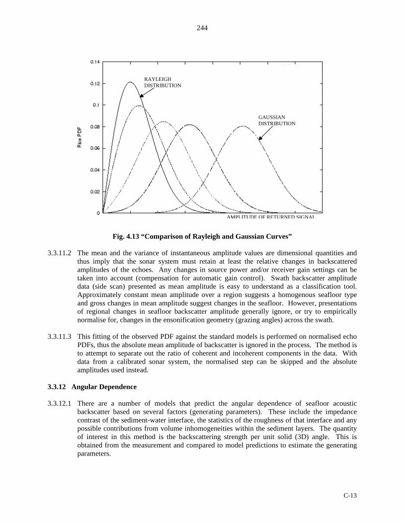
244

C-13

Fig. 4.13 “Comparison of Rayleigh and Gaussian Curves” 3.3.11.2 The mean and the variance of instantaneous amplitude values are dimensional quantities and

thus imply that the sonar system must retain at least the relative changes in backscattered amplitudes of the echoes. Any changes in source power and/or receiver gain settings can be taken into account (compensation for automatic gain control). Swath backscatter amplitude data (side scan) presented as mean amplitude is easy to understand as a classification tool. Approximately constant mean amplitude over a region suggests a homogenous seafloor type and gross changes in mean amplitude suggest changes in the seafloor. However, presentations of regional changes in seafloor backscatter amplitude generally ignore, or try to empirically normalise for, changes in the ensonification geometry (grazing angles) across the swath.

3.3.11.3 This fitting of the observed PDF against the standard models is performed on normalised echo

PDFs, thus the absolute mean amplitude of backscatter is ignored in the process. The method is to attempt to separate out the ratio of coherent and incoherent components in the data. With data from a calibrated sonar system, the normalised step can be skipped and the absolute amplitudes used instead.

3.3.12 Angular Dependence 3.3.12.1 There are a number of models that predict the angular dependence of seafloor acoustic

backscatter based on several factors (generating parameters). These include the impedance contrast of the sediment-water interface, the statistics of the roughness of that interface and any possible contributions from volume inhomogeneities within the sediment layers. The quantity of interest in this method is the backscattering strength per unit solid (3D) angle. This is obtained from the measurement and compared to model predictions to estimate the generating parameters.

GAUSSIAN DISTRIBUTION

RAYLEIGH DISTRIBUTION

AMPLITUDE OF RETURNED SIGNAL

245

C-13

3.3.12.2 High aspect ratio systems such as MBES provide measurements of the backscattered amplitude at grazing angles ranging from 90° (vertical) through grazing angles as low as 15°. This is in contrast to the distribution of grazing angles recovered by deep-towed, low aspect ratio SSS, which tend to be biased to very low angles.

3.3.12.3 Commensurate with this method is the requirement to know the ray path of the acoustic energy

as it strikes the seafloor and the 3D slope of the seafloor interface that it strikes. This leads to assigning an instantaneous measure of backscatter amplitude to that angle. In order to arrive at a good estimate of the mean backscatter strength at that grazing angle, a large number (>10) of instantaneous measurements are used. This obviously assumes the seafloor under investigation is not changing over the length of the MBES swath (i.e. the seafloor type is the same from nadir to the far range).

3.3.13 Acoustic Backscatter Data Interpretation 3.3.13.1 In the first instance, interpretation of a digital side scan image is often difficult. At the very

limit of resolution is the single instantaneous sample of backscatter intensity. This is derived from a complex sum of all the individual scattered contributions from within the ensonified area and also the scattered contributions from the volume of sediment below the ensonified area. Notwithstanding the derived solution, there are three main effects that are noticeable in any side scan mosaic:

• variations in backscatter strength due to changing seafloor type; • variations in backscatter strength due to changes in seafloor slope; • true cast shadows. 3.3.13.2 For conventional SSS the first two are ambiguous. There is no way to unambiguously tell

whether fluctuations are due to slope or texture. In reality it is rare to see a significant change in the seafloor slope without a change in texture. In contrast to conventional SSS, swath sonar systems can resolve the ambiguity for those cases where the topographic wavelength is greater than the beam spacing, although roughness at shorter wavelengths cannot be resolved.

3.3.13.3 True cast shadows can be recognised by both systems as long as the signal-to-noise ration is

high enough - thus the drop in signal strength is greater than that expected for any real sediment type. Interestingly, swath sonars cannot predict the presence of a shadow from the topographic information alone. This is because a shadow implies slopes steeper than the ray path and thus swath sonars cannot see behind the shadowing feature. This is important to remember when using side angular sectors. Steep topography facing away from the sonar is not adequately resolved and thus the resulting derived terrain model will be distorted. Even with swath sonars, it is often not clear whether short wavelength variations in seafloor backscatter are a result of either of the above effects. The only way to resolve this is to image the seafloor from multiple near-orthogonal directions.

3.3.13.4 First and foremost, the surveyor is concerned about verifying potential hydrographic hazards on

the seafloor. Any confirmation or denial of the validity of an anomalous sounding represents an aid in the interpretation of the data. This ultimately allows greater confidence in the quality of the sounding data which will appear on a navigation chart. As we have seen there are resolution limitations to high-speed MBES imagery, which means that you cannot always

246

C-13

resolve the discrete hydrographic anomalies that are of interest. This lends to the discussion of deploying conventional, towed SSS in conjunction with a swath sonar system.

3.3.13.5 When the beam reaches the seafloor some of the beam is reflected back in the form of an echo,

but much of the energy is scattered in all directions, and some is even absorbed into the seafloor. The vertical incidence case is concerned mainly with the reflection properties of the seafloor, and again, different characteristics of the echosounder beam have an effect on the amount of the signal that is reflected. The frequency of the signal is one of the most important attributes in this respect. The MBES case is more complicated and the scattering properties of the seafloor take on a larger importance.

3.3.13.6 Returns from a smooth hard seafloor. As the sound wave travels through the water, it moves by

displacing water particles, causing them to vibrate and so allow the passage of the wave. The water has a low acoustic impedance, or a low resistance to the movement of the wave. When the wave reaches the seafloor however, the seafloor has a high acoustic impedance and does not allow the sound wave to continue into the seafloor. The particles are densely packed and are not able to move easily. Since the total energy must be maintained and the energy cannot pass into the seafloor in the form of a sound wave, it must go somewhere and the result is that it is radiated back into the water. Some, probably a small percentage, will be reflected back in the direction of the incoming wave and will travel back to be received at the sonar transducer as an echo.

3.3.13.7 Effects of different types of seafloor and differing angles of incidence. Different types of

seafloor will have different levels of acoustic impedance. If the level is low then some of the sound energy is absorbed into the seafloor and the returning echo will be weaker. If the level is high then more is reflected. Similarly, the intensity of the reflected signal is also dependant on the angle of incidence. If the angle is high, approaching 90°, then a large part of the sound wave will be reflected back towards the sonar. If the angle is low then the major part of the sound wave will be scattered in a direction away from the transducer, however some will still return as a weak echo.

3.3.13.8 The type of seafloor will have an effect on the returning signal as well. The relationship

between the angle of incidence, the type of seafloor and the level of the returning signal is not a straightforward one. For the beam arriving at a low level of incidence, if the seafloor is rough then there will be more faces that are near to a right angle to the incoming sound wave and therefore give a stronger reflection. A smooth seafloor will in general result in more of the signal being scattered in other directions and not back in the direction of the sonar receiver. For a high angle of incidence, however, the situation is likely to be reversed and a smooth seafloor may give a better return. This will however depend on a number of factors such as particle size and the composition of the seafloor.

3.3.14 Military Classification Models 3.3.14.1.1 In preparing a military classification (or texture) model from the sonar records the first task for

the surveyor is to decide whether the texture of the seafloor is mud, sand, gravel or rock. It is appreciated that the seafloor contains a wide variety of combinations of the four basic categories, but more detailed analysis is best undertaken by written descriptions. Clearly defined boundaries between different types of seafloor should be shown as firm lines and ill-defined limits should be depicted as pecked lines. Figure 4.14 shows an example of a military classification model.

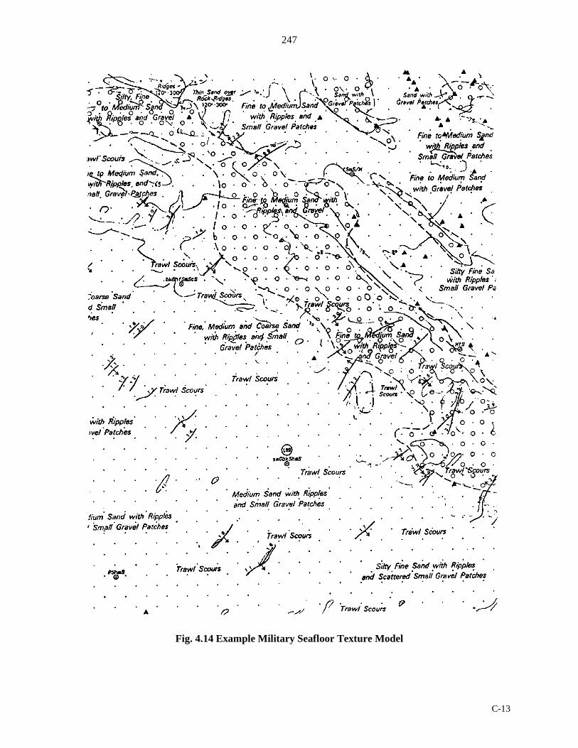
247

C-13

Fig. 4.14 Example Military Seafloor Texture Model

248

C-13

3.3.14.2 The graphic representation of the seafloor texture should be amplified by use of written descriptions. Examples of the terms to be used, together with their definitions follow. It is stressed that these are not exhaustive; other words may be used providing the meaning is clear to all who may use the information. Descriptions of “negative” features (for example “flat featureless sand”) are as useful as information on more prominent characteristics. Written descriptions should be kept brief.

3.3.14.3 Features such as wrecks, sand-waves, trawl scours and pipelines also form an important part of

the description of the seafloor. These features are invariably more important than written descriptions and in congested areas their inclusion should take priority.

3.3.14.4 Sandwaves are a common feature of seafloor topography and may occur either as isolated

features or in fields. Different symbols are used for each type: • Isolated sandwaves. To ensure accuracy, the position of the crest of the wave must be

plotted from the echo-trace and not from the sonar record. The symbol for an isolated sandwave is then to be positioned along the line of the crest. If the wave is asymmetric, a small arrow is to be inserted pointing down the steeper side of the feature, the arrow should be omitted if the wave is symmetrical. Details of the height of the crest above the trough should be included.

• Sandwave fields. Many sandwaves occur in groups with similar height and orientation.

Under these conditions individual waves need not be plotted. The extent of the field should be delineated, again referring to the echo-trace for accuracy and the symbol for a sandwave field inserted. The orientation of the crests should be indicated, as should the wavelength, height, symmetry and the steeper side.

3.3.14.5 For plotting purposes, a sandwave is defined as having a height greater than one metre.

Features smaller than this should be classed as ripples. The wavelength is defined as the distance between two adjacent crests; the height is the difference in depth between a crest and its adjacent trough. As a rule of thumb, crests which plot closer together than one centimetre on paper and are similar in orientation, height and wavelength should be considered a field. Ripples are often superimposed on waves and may have a different orientation a brief written description such as “Ripples 120/300” should be placed next to the sand-wave symbol.

3.3.14.6 Small sea floor contacts. All non-ephemeral contacts larger than one metre must be plotted.

Where more than five such contacts exist per square centimetre the area may be delineated and a notation made. Wherever possible the number of contacts in each area should be stated, written descriptions may be included where useful.

3.3.14.7 Wrecks and obstructions. All wrecks and obstructions located during the survey must be

included in the classification model. Wrecks are to be shown by the “non dangerous” wreck symbol, oriented in the same direction as the wreck. The extent and direction of any scour is to be noted, e.g. ‘Scour 155/50m’. Other obstructions are to be shown using the “foul” symbol, with a written description if possible, e.g. ‘wellhead’.

3.3.14.8 Small depressions. Certain areas of seafloor may contain small depressions, distinguishable on

the sonar trace by the “shadow” being in front of the contact. Some may show a pronounced lip and include “pock-marks”. Unless their origin is known (for example if an oil-rig is moved during a survey) classification should not be attempted.

249

C-13

3.3.14.9 Trawl scours. In many areas, trawl scours are a frequent and distinctive part of the seafloor. Their importance is increased by the fact that they are most often met in otherwise flat areas. Isolated trawl scours are to be shown individually; concentrations of them may be delineated and the wording "numerous trawl scours" inserted.

3.3.14.10 Pipelines. All pipelines detected during a survey are to be plotted. Areas of buried pipe should

not be interpolated unless they are visible on the SSS trace, in this event the word “buried” is to be inserted as required. Pipes which stand proud of the seafloor are to have their height in metres noted at intervals.

3.3.14.11 Depth contours. Contours are to be included with the normal vertical interval being five

metres. In areas where a large range of depth occurs this may be expanded at the discretion of the surveyor, providing the presentation of the “form” of the texture is maintained. The purpose of drawing the depth contours is to assist the surveyor in his interpretation of the sonograph.

3.3.14.12 Descriptions for use on Military Seafloor Classification Models: Sandwaves. Straight or sinuous ridges of sand commonly aligned across the dominant tidal

stream or current. Minimum height is one metre. Crest separation (wavelength) can be up to 1000 m with heights reaching 20 m. May be symmetrical or asymmetrical, and may have ripples on them.

Ripples. Small ridges of sand, similar in shape to sandwaves but with a height of less than one

metre. Usually orientated transverse to the tidal or current flow with wavelength of less than 15 m. May not be detectable with an echo sounder.

Furrows & Ridges. Longitudinal bed-forms in gravel, sand or mud, some of which can be 9 km

long and up to 14 m wide. They may be solitary, but more usually occur in groups. They are generally parallel to the prevailing currents.

Sand Ribbons. Normally apparent overlying a coarser type of seafloor. Most are straight and

parallel with currents. Can be up to 15 km long, 200 m wide and are generally only a few centimetres thick. Typically have a "laddered” appearance due to the presence of ripples.

Gravel/ Sand/ Mud Patches. Thinly-spread patches of gravel, sand or mud no more than 100 m

across and commonly less than 2 m thick. May be depositional and subject to movement. Shape may be determined by the relief of the underlying seafloor.

Rock Outcrop. A patch of rock covering a small area. Refers to a cohesive group, not a

collection of boulders. Pinnacle. A rock of limited horizontal extent with height considerably greater than surrounding

rocks. Ledge. Rock outcrop with length in excess of 300 m and relatively narrow in comparison.

Often found in groups, with similar direction and extent.

250

C-13

Bank. Usually of sand or gravel, but may be of rock. A rise in the seafloor over a relatively small area, but fairly prominent in relation to its surroundings. When formed of sediment it is often oriented along the tidal flow.

Large/ Small. Preferred to big, great, high/little, slight, mini, etc. Broad/ Narrow. Used to express width when qualifying such features as sand ribbons. Broad

should only be used for ribbons over 150 m wide, narrow for those less than 10 m wide. Smooth. Preferred to even or level, and may refer to a seafloor that is either flat or sloping.

Will usually refer only to mud. Flat. Must only be used to describe level surfaces (i.e. no significant gradient). Sloping. Refers to any area where there is a general trend in the depth of the seafloor, i.e. a sea

floor gradient. A sloping seafloor may be smooth but cannot be flat. Gentle. Gradual, slowly changing. Regular. Used to qualify a series of features which are uniform in amplitude and wavelength,

i.e. sandwaves, ridges. Irregular. Used to qualify features which are not uniform but do have a specific entity, i.e.

sandwaves. Can also be used to describe an area of rock where no regular structure is evident. Prominent. Used to describe a feature or series of features which is or are very obvious in

relation to their general surroundings. Featureless. Applied normally to either a flat or smooth seafloor where the featureless aspect is

either unusual or of considerable extent.

251

C-13

3.3.14.13 Symbols for use on Military Seafloor Classification Models are at Figure 4.15:

Fig. 4.15 Symbols for use on Military Seafloor Classification Models

Rock exposure Gravel Sand Mud Clearly defined seafloor texture boundary Ill-defined seafloor texture boundary Sand-wave crest with crest-to-trough height in metres, symbol denotes direction of steepest side Sand-wave areas (with height, orientation, wavelength and symmetry; A = Asymmetrical; S = Symmetrical)

Prominent trawl scour

Area of concentrated trawl scours

Significant sonar contact

Patch of highly reflective seafloor without significant height or extent

Pockmark

Position of seafloor sample with abbreviated description and identifying number if retained Wreck, orientated as appropriate, with direction and extent of scour Foul or obstruction (with classification if applicable) Submerged well Pipeline Seafloor contour at 5 m vertical intervals.

252

C-13

REFERENCES

1987 “The Use of Side Scan Sonar for Hydrographic Surveying and the Gathering of Bottom Texture Information”

UK Hydrographic Department Professional Paper No. 24

1990 “Sound Underwater Images” – A Guide to the Generation and Interpretation of Side Scan Sonar Data.

Fish JP & Carr HA

1994 “High Frequency Ocean Environmental Acoustic Models Handbook”

Washington University Seattle Applied Physics Lab

1997 “Admiralty Manual of Hydrographic Surveying” UK Hydrographic Office

1998 “Side Scan Versus MBES Object Detection - A Comparative Analysis”

Brissette MB & Hughes Clarke JE

2001 “LEEUWIN Class Operating System” Australian Hydrographic Service

2004 “Hydrographic Quality Assurance Instructions for Admiralty Surveys”

UK Hydrographic Office

__________