science assessment team #3 - ska indico (indico) · annalisa bonafede & chiara ferrari (with...

Chiara Ferrari (ObsCoAz, Chair)

Leon Koopmans (UGroningen)

James Aguirre (UPenn)

Annalisa Bonafede (INAF)

Francesco de Gasperin (ULeiden)

Jason Hessels (UAmsterdam/ASTRON)

Divya Oberoi (NCRA-TIFR)

Philippe Zarka (ObsPM)

Anna Bonaldi (SKAO Support)

Science Assessment Team #3

- Impact of SKA1-Low frequency optimisation -

The team acknowledges the work of:

F. Vazza

(cosmic-web filament detectability)

L. Levin Preston

(pulsar yields simulations)

S. Wijnholds

(discussions about calibration)

Objectives of the SAT#3Assess if and how:

• the reduction of the optimised frequency coverage of SKA1-LOW from 100-300 MHz to 100-200 MHz

• a significantly reduced sensitivity (>50%) above 250 MHz

would have a major impact on our different science cases:

• EoR/CD

• pulsars

• transient

• planets

• solar physics

• large scale structures

At this stage, we have to take into account any other possible SKA1-LOW change

listed in the document Cost Control Plan Explanation (CCPE) only if it affects our estimates of the previous point

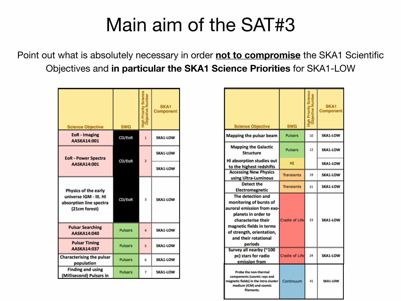
Main aim of the SAT#3Point out what is absolutely necessary in order not to compromise the SKA1 Scientific

Objectives and in particular the SKA1 Science Priorities for SKA1-LOW

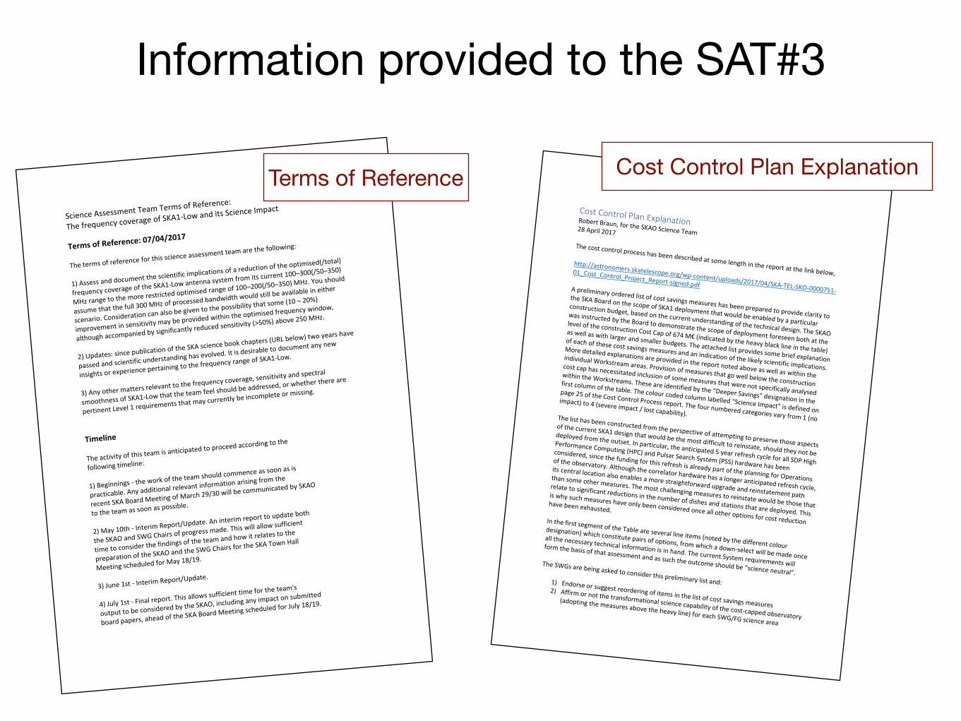
Information provided to the SAT#3

ScienceAssessmentTeamTermsofReference:

ThefrequencycoverageofSKA1-Low

anditsScienceImpact

TermsofReference:07/

04/2017

Thetermsofreferencefort

hisscienceassessmentteamarethefollowing:

1)Assessanddocu

mentthescientificimplicationsofaredu

ctionoftheoptimised(/total)

frequencycoverageoftheSKA1-Low

antennasystemfromitscurrent100–300(/50–350)

MHzrangetothemorerestrictedoptimisedrangeof100–

200(/50–350)MHz.Youshould

assumethatthefull300MHzofprocessedba

ndwidthwouldstillbeavailableineit

her

scenario.Considerationcanalsobeg

iventothepossibilitythatsome(10–20%)

improvementinsensitivitymaybeprovidedwit

hintheoptimisedfrequencywindow,

althoughaccompaniedbysignificantlyreducedsensi

tivity(>50%)above250MHz.

2)Updates:sincep

ublicationoftheSKAsciencebookch

apters(URLbelow)twoyearshave

passedandscientificunderstandingh

asevolved.Itisdesirabletodocumentanynew

insightsorexperiencepertainingtot

hefrequencyrangeofSKA1-Low.

3)Anyothermattersrelevanttot

hefrequencycoverage,sensitivityan

dspectral

smoothnessofSKA1-Lowthattheteam

feelshouldbeaddressed,orwhether

thereare

pertinentLevel1requirementsthatmaycurrentlybeinc

ompleteormissing.

TimelineTheactivityofthis

teamisanticipatedtoproceedaccordingt

othe

followingtimeline:

1)Beginnings-the

workoftheteamshouldcommenceassoonasis

practicable.Anyadditionalrelevantin

formationarisingfromthe

recentSKABoardMeetingofMarch29/30willbe

communicatedbySKAO

totheteamassoonaspossible.

2)May10th-InterimReport/Update.A

ninterimreporttoupdateboth

theSKAOandSWGChairsofprogressmade.Thiswillallow

sufficient

timetoconsiderthefindingsoftheteam

andhowitrelatestothe

preparationoftheSKAOandtheSW

GChairsfortheSKATownHall

MeetingscheduledforMay18/19.

3)June1st-Interim

Report/Update.

4)July1st-Finalre

port.Thisallowssufficienttimefortheteam's

outputtobeconsideredbytheSKAO

,includinganyimpactonsubmitted

boardpapers,aheadoftheSKABoar

dMeetingscheduledforJuly18/19.

Terms of ReferenceCostControlPlanExplanationRobertBraun,fortheSKAOScienceTeam28April2017Thecostcontrolprocesshasbeendescribedatsomelengthinthereportatthelinkbelow,

http://astronomers.skatelescope.org/wp-content/uploads/2017/04/SKA-TEL-SKO-0000751-

01_Cost_Control_Project_Report-signed.pdfApreliminaryorderedlistofcostsavingsmeasureshasbeenpreparedtoprovideclarityto

theSKABoardonthescopeofSKA1deploymentthatwouldbeenabledbyaparticular

constructionbudget,basedonthecurrentunderstandingofthetechnicaldesign.TheSKAO

wasinstructedbytheBoardtodemonstratethescopeofdeploymentforeseenbothatthe

leveloftheconstructionCostCapof674M€(indicatedbytheheavyblacklineinthetable)

aswellaswithlargerandsmallerbudgets.Theattachedlistprovidessomebriefexplanation

ofeachofthesecostsavingsmeasuresandanindicationofthelikelyscientificimplications.

Moredetailedexplanationsareprovidedinthereportnotedaboveaswellaswithinthe

individualWorkstreamareas.Provisionofmeasuresthatgowellbelowtheconstruction

costcaphasnecessitatedinclusionofsomemeasuresthatwerenotspecificallyanalysed

withintheWorkstreams.Theseareidentifiedbythe“DeeperSavings”designationinthe

firstcolumnofthetable.Thecolourcodedcolumnlabelled“ScienceImpact”isdefinedon

page25oftheCostControlProcessreport.Thefournumberedcategoriesvaryfrom1(no

impact)to4(severeimpact/lostcapability).Thelisthasbeenconstructedfromtheperspectiveofattemptingtopreservethoseaspects

ofthecurrentSKA1designthatwouldbethemostdifficulttoreinstate,shouldtheynotbe

deployedfromtheoutset.Inparticular,theanticipated5yearrefreshcycleforallSDPHigh

PerformanceComputing(HPC)andPulsarSearchSystem(PSS)hardwarehasbeen

considered,sincethefundingforthisrefreshisalreadypartoftheplanningforOperations

oftheobservatory.Althoughthecorrelatorhardwarehasalongeranticipatedrefreshcycle,

itscentrallocationalsoenablesamorestraightforwardupgradeandreinstatementpath

thansomeothermeasures.Themostchallengingmeasurestoreinstatewouldbethosethat

relatetosignificantreductionsinthenumberofdishesandstationsthataredeployed.This

iswhysuchmeasureshaveonlybeenconsideredonceallotheroptionsforcostreduction

havebeenexhausted.InthefirstsegmentoftheTableareseverallineitems(notedbythedifferentcolour

designation)whichconstitutepairsofoptions,fromwhichadown-selectwillbemadeonce

allthenecessarytechnicalinformationisinhand.ThecurrentSystemrequirementswill

formthebasisofthatassessmentandassuchtheoutcomeshouldbe“scienceneutral”.

TheSWGsarebeingaskedtoconsiderthispreliminarylistand:

1) Endorseorsuggestreorderingofitemsinthelistofcostsavingsmeasures

2) Affirmornotthetransformationalsciencecapabilityofthecost-cappedobservatory

(adoptingthemeasuresabovetheheavyline)foreachSWG/FGsciencearea

Cost Control Plan Explanation

Information provided to the SAT#3

Provided by SKAO

Cost Control Plan Explanation

Q & A with SKAO

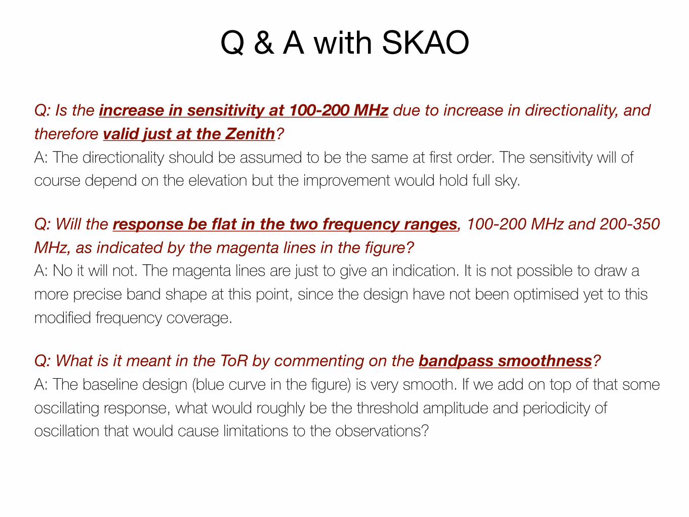
Q: Is the increase in sensitivity at 100-200 MHz due to increase in directionality, and therefore valid just at the Zenith? A: The directionality should be assumed to be the same at first order. The sensitivity will of course depend on the elevation but the improvement would hold full sky.

Q: Will the response be flat in the two frequency ranges, 100-200 MHz and 200-350 MHz, as indicated by the magenta lines in the figure? A: No it will not. The magenta lines are just to give an indication. It is not possible to draw a more precise band shape at this point, since the design have not been optimised yet to this modified frequency coverage.

Q: What is it meant in the ToR by commenting on the bandpass smoothness? A: The baseline design (blue curve in the figure) is very smooth. If we add on top of that some oscillating response, what would roughly be the threshold amplitude and periodicity of oscillation that would cause limitations to the observations?

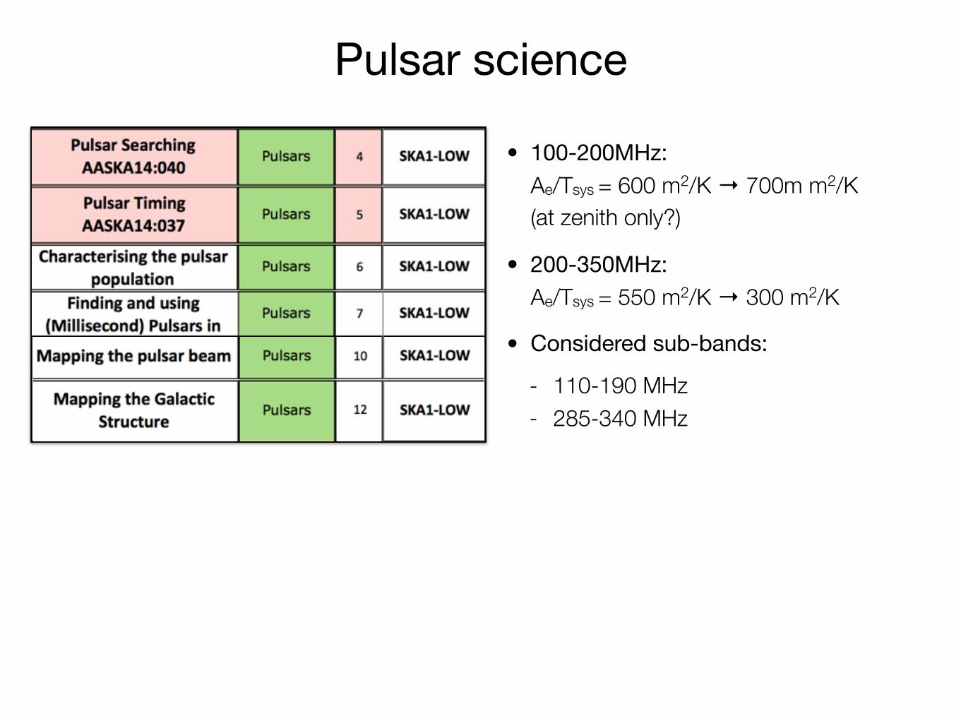
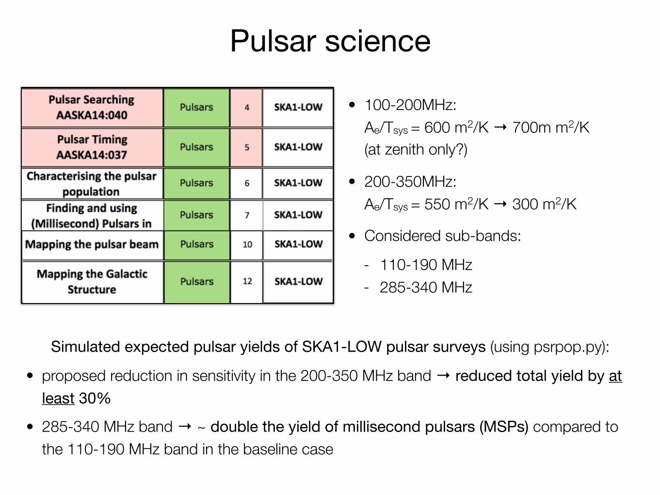
Pulsar science

• 100-200MHz: Ae/Tsys = 600 m2/K → 700m m2/K (at zenith only?)

• 200-350MHz: Ae/Tsys = 550 m2/K → 300 m2/K

• Considered sub-bands:

- 110-190 MHz - 285-340 MHz

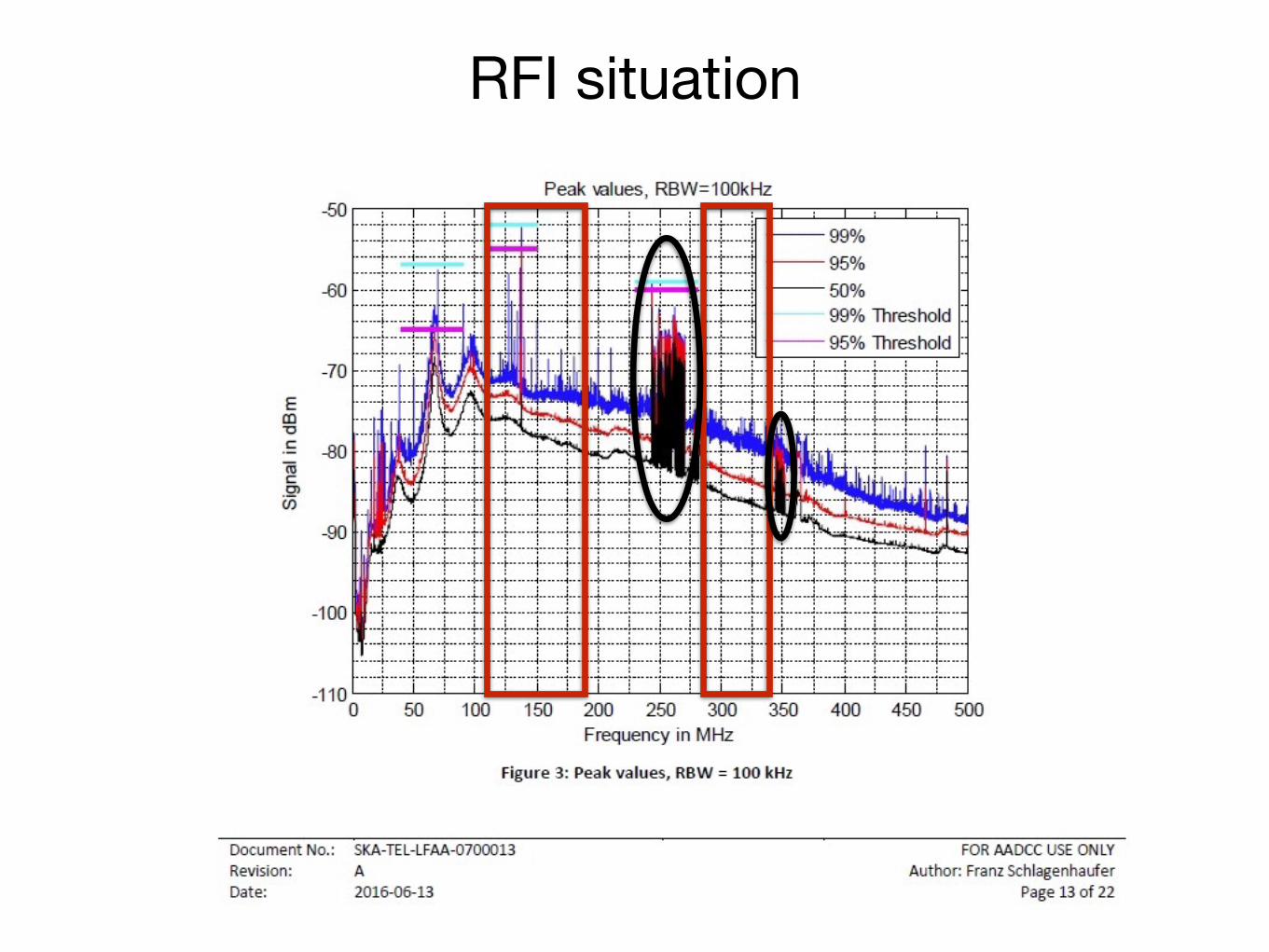
RFI situation

Pulsar science

• 100-200MHz: Ae/Tsys = 600 m2/K → 700m m2/K (at zenith only?)

• 200-350MHz: Ae/Tsys = 550 m2/K → 300 m2/K

• Considered sub-bands:

- 110-190 MHz - 285-340 MHz

Simulated expected pulsar yields of SKA1-LOW pulsar surveys (using psrpop.py):

• proposed reduction in sensitivity in the 200-350 MHz band → reduced total yield by at least 30%

• 285-340 MHz band → ~ double the yield of millisecond pulsars (MSPs) compared to the 110-190 MHz band in the baseline case

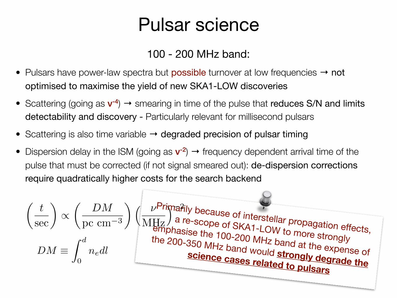
Pulsar science100 - 200 MHz band:

• Pulsars have power-law spectra but possible turnover at low frequencies → not optimised to maximise the yield of new SKA1-LOW discoveries

• Scattering (going as ν-4) → smearing in time of the pulse that reduces S/N and limits detectability and discovery - Particularly relevant for millisecond pulsars

• Scattering is also time variable → degraded precision of pulsar timing

• Dispersion delay in the ISM (going as ν-2) → frequency dependent arrival time of the pulse that must be corrected (if not signal smeared out): de-dispersion corrections require quadratically higher costs for the search backend

Primarily because of interstellar propagation effects, a re-scope of SKA1-LOW to more strongly

emphasise the 100-200 MHz band at the expense of the 200-350 MHz band would strongly degrade the

science cases related to pulsars

✓t

sec

◆/

✓DM

pc cm�3

◆⇣ ⌫

MHz

⌘�2

DM ⌘Z d

0nedl

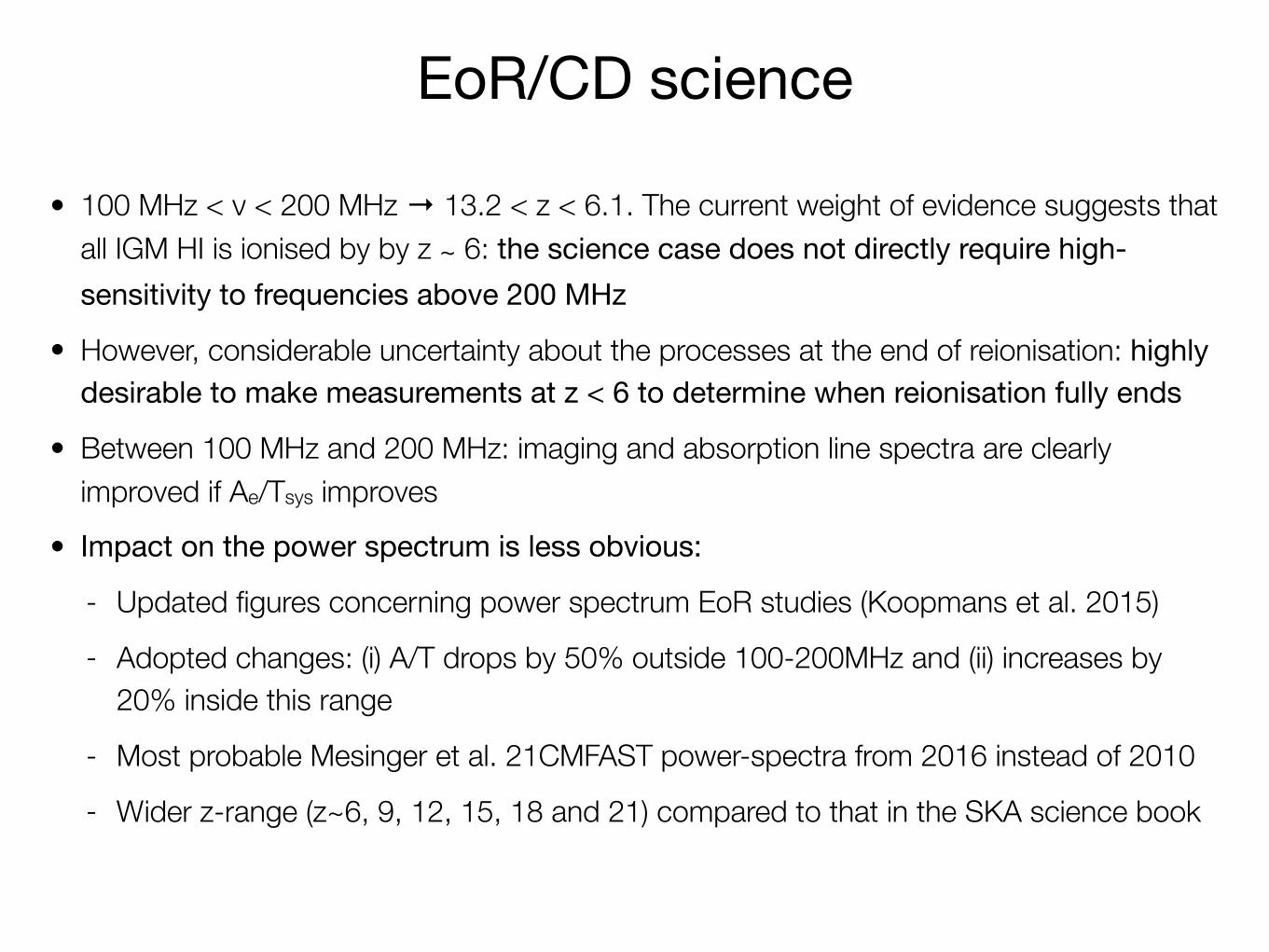
EoR/CD science

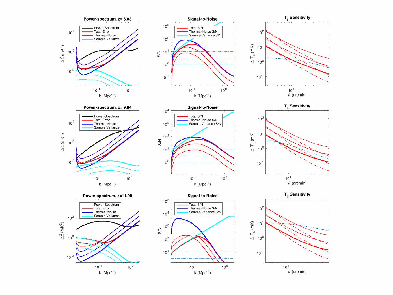
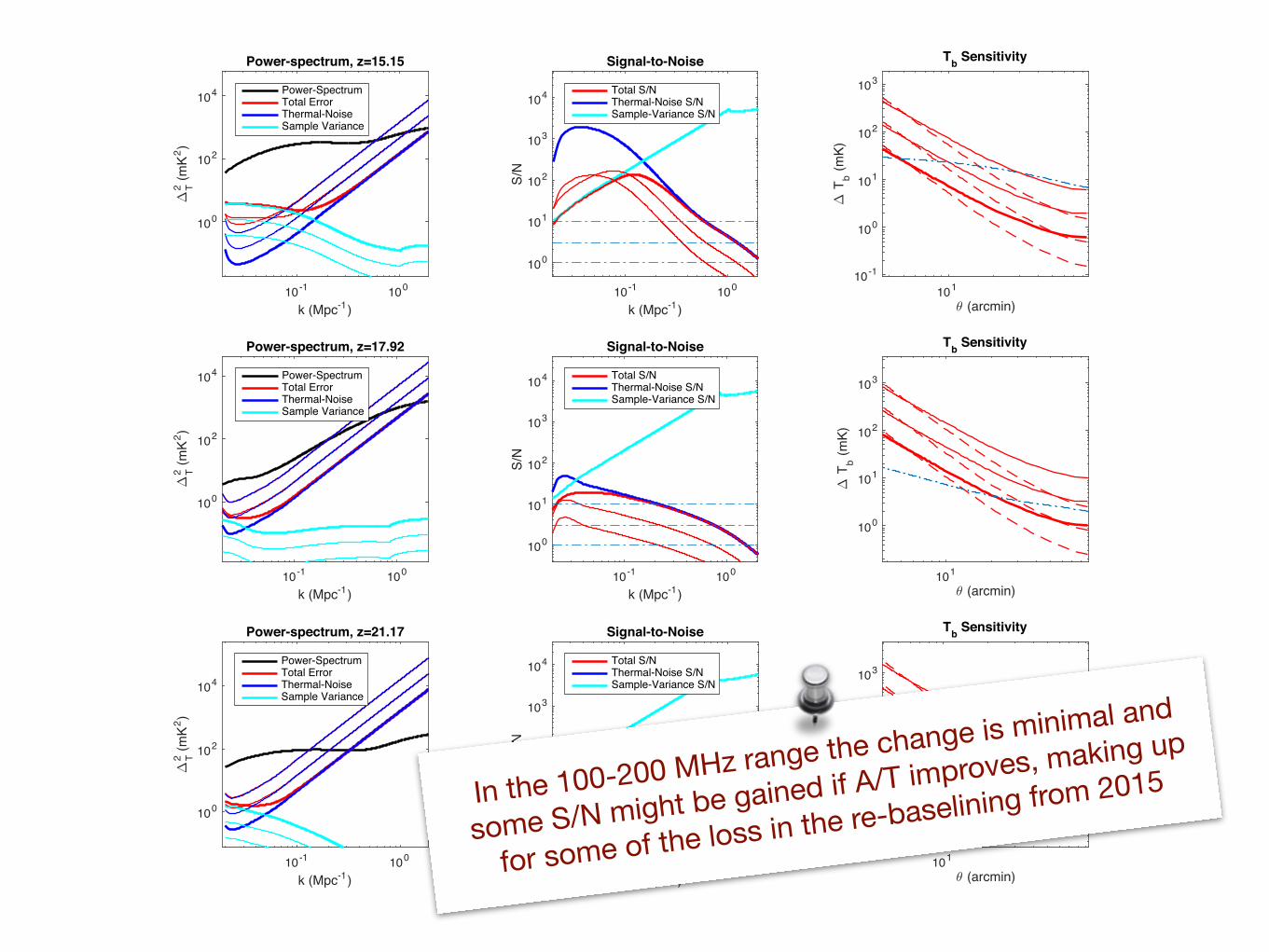
• 100 MHz < ν < 200 MHz → 13.2 < z < 6.1. The current weight of evidence suggests that all IGM HI is ionised by by z ∼ 6: the science case does not directly require high-sensitivity to frequencies above 200 MHz

• However, considerable uncertainty about the processes at the end of reionisation: highly desirable to make measurements at z < 6 to determine when reionisation fully ends

• Between 100 MHz and 200 MHz: imaging and absorption line spectra are clearly improved if Ae/Tsys improves

• Impact on the power spectrum is less obvious:

- Updated figures concerning power spectrum EoR studies (Koopmans et al. 2015)

- Adopted changes: (i) A/T drops by 50% outside 100-200MHz and (ii) increases by 20% inside this range

- Most probable Mesinger et al. 21CMFAST power-spectra from 2016 instead of 2010

- Wider z-range (z~6, 9, 12, 15, 18 and 21) compared to that in the SKA science book

10-1 100

k (Mpc-1)

10-2

100

102

∆2 T (m

K2 )

Power-spectrum, z= 6.03

Power-SpectrumTotal ErrorThermal-NoiseSample Variance

10-1 100

k (Mpc-1)

10-2

100

102

∆2 T (m

K2 )

Power-spectrum, z= 9.04


10-1 100

k (Mpc-1)

10-2

100

102

∆2 T (m

K2 )

Power-spectrum, z=11.99


10-1 100

k (Mpc-1)

10-1

100

101

102

103

S/N

Signal-to-Noise

Total S/NThermal-Noise S/NSample-Variance S/N

10-1 100

k (Mpc-1)

100

101

102

103

104

S/N

Signal-to-Noise


10-1 100

k (Mpc-1)

101

102

103

104

105

S/N

Signal-to-Noise


101

θ (arcmin)

10-1

100

101

102

∆ T

b (mK)

Tb Sensitivity

101

θ (arcmin)

10-1

100

101

102

∆ T

b (mK)

Tb Sensitivity

101

θ (arcmin)

10-1

100

101

102

∆ T

b (mK)

Tb Sensitivity

10-1 100

k (Mpc-1)

100

102

104

∆2 T (m

K2 )



10-1 100

k (Mpc-1)

100

102

104

∆2 T (m

K2 )



10-1 100

k (Mpc-1)

100

102

104

∆2 T (m

K2 )



10-1 100

k (Mpc-1)

100

101

102

103

104

S/N

Signal-to-Noise


10-1 100

k (Mpc-1)

100

101

102

103

104

S/N

Signal-to-Noise


10-1 100

k (Mpc-1)

100

101

102

103

104

S/N

Signal-to-Noise


101

θ (arcmin)

10-1

100

101

102

103

∆ T

b (mK)

Tb Sensitivity

101

θ (arcmin)

100

101

102

103

∆ T

b (mK)

Tb Sensitivity

101

θ (arcmin)

100

101

102

103

∆ T

b (mK)

Tb Sensitivity

In the 100-200 MHz range the change is minimal and

some S/N might be gained if A/T improves, making up

for some of the loss in the re-baselining from 2015

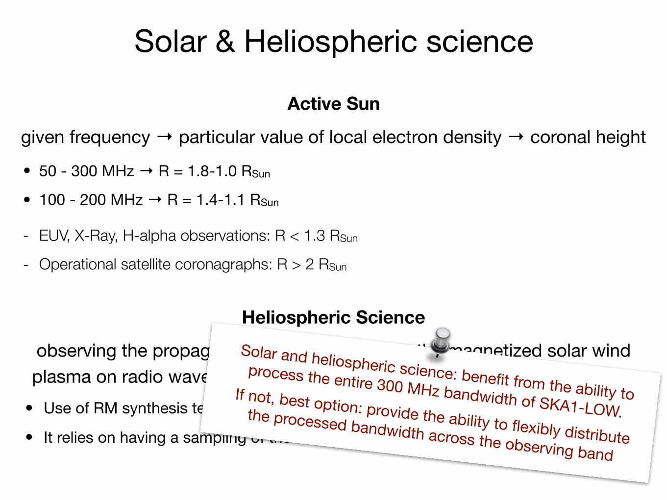
Solar & Heliospheric science

Active Sun

given frequency → particular value of local electron density → coronal height

• 50 - 300 MHz → R = 1.8-1.0 RSun

• 100 - 200 MHz → R = 1.4-1.1 RSun

- EUV, X-Ray, H-alpha observations: R < 1.3 RSun

- Operational satellite coronagraphs: R > 2 RSun

Solar & Heliospheric science

Active Sun

given frequency → particular value of local electron density → coronal height

• 50 - 300 MHz → R = 1.8-1.0 RSun

• 100 - 200 MHz → R = 1.4-1.1 RSun

- EUV, X-Ray, H-alpha observations: R < 1.3 RSun

- Operational satellite coronagraphs: R > 2 RSun

Heliospheric Science

observing the propagation effects imposed by the magnetized solar wind plasma on radio waves from the distant background cosmic radio sources

• Use of RM synthesis technique

• It relies on having a sampling of the RM across a large wavelength range

Solar and heliospheric science: benefit from the ability to process the entire 300 MHz bandwidth of SKA1-LOW.

If not, best option: provide the ability to flexibly distribute the processed bandwidth across the observing band

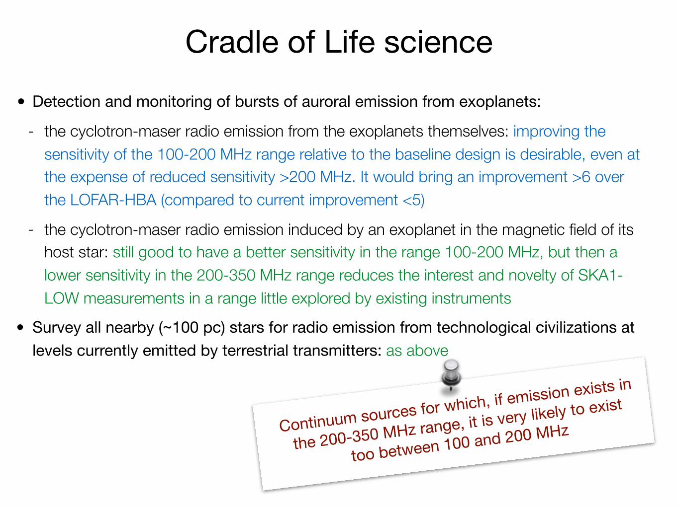
Cradle of Life science

Continuum sources for which, if emission exists in

the 200-350 MHz range, it is very likely to exist

too between 100 and 200 MHz

• Detection and monitoring of bursts of auroral emission from exoplanets:

- the cyclotron-maser radio emission from the exoplanets themselves: improving the sensitivity of the 100-200 MHz range relative to the baseline design is desirable, even at the expense of reduced sensitivity >200 MHz. It would bring an improvement >6 over the LOFAR-HBA (compared to current improvement <5)

- the cyclotron-maser radio emission induced by an exoplanet in the magnetic field of its host star: still good to have a better sensitivity in the range 100-200 MHz, but then a lower sensitivity in the 200-350 MHz range reduces the interest and novelty of SKA1-LOW measurements in a range little explored by existing instruments

• Survey all nearby (~100 pc) stars for radio emission from technological civilizations at levels currently emitted by terrestrial transmitters: as above

Large scale structures

Tuesday 2 May 2017

Science Assessment Team Terms of Reference:The frequency coverage of SKA1-Low and its Science Impact - Imaging & continuumAnnalisa Bonafede & Chiara Ferrari (with contribution from Franco Vazza)

General considerations:

- With the reduction of the optimised band (100-200) versus (100-300) confusion noise will be reached faster, resolution will degrade slightly, integration time to reach the same thermal noise will increase.

- Some of these aspects would become critical if also the maximum bandwidth is reduced (see “Other considerations” below)

Considerations for the scientific case “detection of the comic web” - and update on the SKA chapter by Vazza et al.( 2015) and detection of cluster outskirts.

- Frequency coverage is not essential for the detection of the cosmic web. The low frequency part of the band is more sensitive to large scale structures, and the higher resolution provided by the highest freq band (200-300 MHz) is not essential.

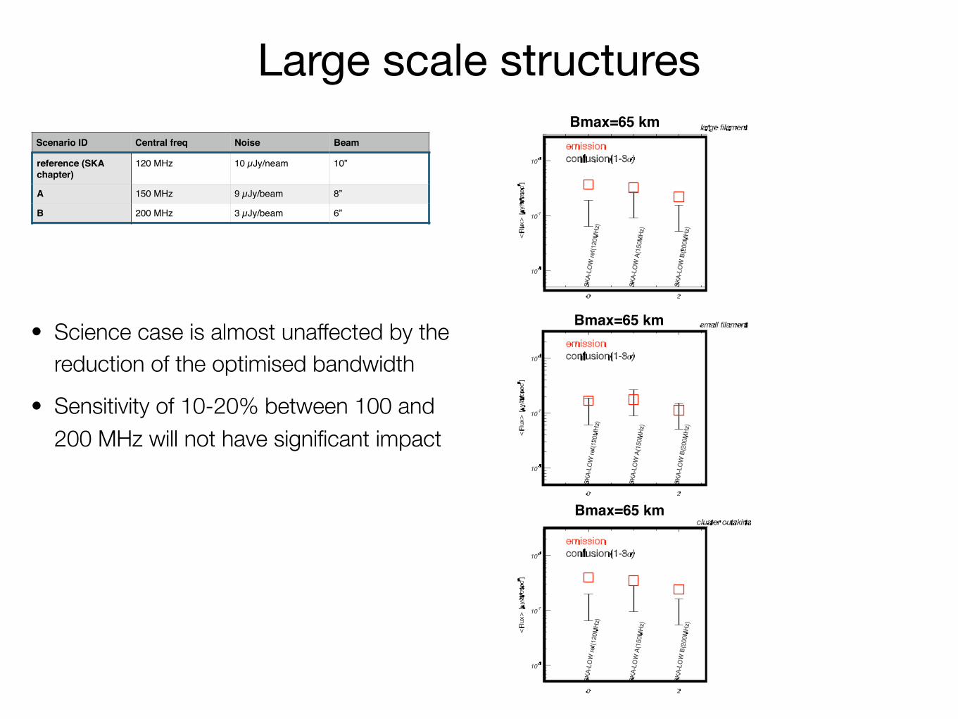
In Fig 1, we show the emission from a cosmic filament taken from a cosmological simulation (same as Vazza et al, 2015 SKA white book). Panel 1 is the figure of reference of the SKA chapter, and other scenarios have been considered as specified in the Table. In the Table and in Figure 2, scenarios that do not consider a change in Bmax are highlighted within boxes. As done for the SKA chapter, we assume that confusion noise will be reached.

�1

Scenario ID Central freq Noise Beam

reference (SKA chapter)

120 MHz 10 µJy/neam 10”

A 150 MHz 9 µJy/beam 8”

B 200 MHz 3 µJy/beam 6”

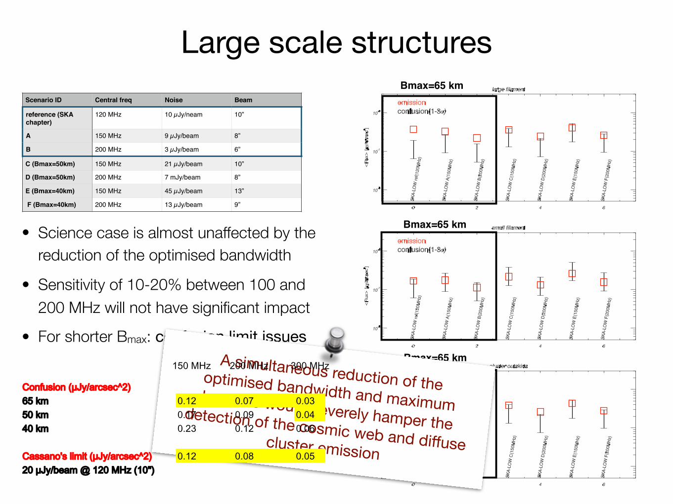
C (Bmax=50km) 150 MHz 21 µJy/beam 10”

D (Bmax=50km) 200 MHz 7 mJy/beam 8”

E (Bmax=40km) 150 MHz 45 µJy/beam 13”

F (Bmax=40km) 200 MHz 13 µJy/beam 9”

Tuesday 2 May 2017

Fig. 1: SKA simulated observations of the cosmic web in the reference scenario (left) A (middle) and B (right). Green contours are gas isodensity contours.

Fig. 2: Top panel:Mean brightnesso of a large filament (white dashed circle in Fig. 1) with a size of 10 Mpc.

Middle panel:Mean brightness of a smaller filament (not shown in Fig. 1), with a size of 1 Mpc

Bottom panel:Mean brightness of a region in the outskirts (around R200) of a massive clusters.

Red squared indicate the emission detected in the simulated image, black bars indicate 1-3 sigma, assuming that the confusion noise is reached. The scenarios listed in the Table are plotted on the x axis.

�2

-9.4 -8.7 -7.9 -7.2 -6.5 -5.8 -5 -4.3 -3.6 -2.8 -2.1

3 degrees

SKA-LOW A (150MHz)

3 degrees

SKA-LOW B(200MHz)

3 degrees

SKA-LOW C (150MHz)

3 degrees

SKA-LOW D (200MHz)

3 degrees

SKA-LOW E (150MHz)

3 degrees

SKA-LOW F(200MHz)

3 degrees

SKA-LOW ref. (120MHz)

Bmax=65 km

Bmax=65 km

Bmax=65 km


Tuesday 2 May 2017








�1










Tuesday 2 May 2017






�2

-9.4 -8.7 -7.9 -7.2 -6.5 -5.8 -5 -4.3 -3.6 -2.8 -2.1

3 degrees

SKA-LOW A (150MHz)

3 degrees

SKA-LOW B(200MHz)

3 degrees

SKA-LOW C (150MHz)

3 degrees

SKA-LOW D (200MHz)

3 degrees

SKA-LOW E (150MHz)

3 degrees

SKA-LOW F(200MHz)

3 degrees


Bmax=65 km

Bmax=65 km

Bmax=65 km

• Science case is almost unaffected by the reduction of the optimised bandwidth

• Sensitivity of 10-20% between 100 and 200 MHz will not have significant impact


Tuesday 2 May 2017








�1










Tuesday 2 May 2017






�2

-9.4 -8.7 -7.9 -7.2 -6.5 -5.8 -5 -4.3 -3.6 -2.8 -2.1

3 degrees

SKA-LOW A (150MHz)

3 degrees

SKA-LOW B(200MHz)

3 degrees

SKA-LOW C (150MHz)

3 degrees

SKA-LOW D (200MHz)

3 degrees

SKA-LOW E (150MHz)

3 degrees

SKA-LOW F(200MHz)

3 degrees


Bmax=65 km

Bmax=65 km

Bmax=65 km

• Science case is almost unaffected by the reduction of the optimised bandwidth

• Sensitivity of 10-20% between 100 and 200 MHz will not have significant impact

• For shorter Bmax: confusion limit issuesA simultaneous reduction of the optimised bandwidth and maximum baseline would severely hamper the

detection of the cosmic web and diffuse cluster emission

' 85L ( 85L ) 85LHFCJ AF "B - - . ) /B ' ' -B '( / )

3F @JHAF 6 "B . - ( .B (' ) ' )B ') ( -

3F @JHAF 6 H ("B '( - )B '- /B () '(

3 HH F H CA A 6 H (" '( . ( 6 0 '( 85L ' "

7941 521 CA A 6 H (" ' .( ' ( -' M. 6 0 '( ' . 85L "

' 85L ( 85L ) 85LHFCJ AF "B - - . ) /B ' ' -B '( / )

3F @JHAF 6 "B . - ( .B (' ) ' )B ') ( -

3F @JHAF 6 H ("B '( - )B '- /B () '(

3 HH F H CA A 6 H (" '( . ( 6 0 '( 85L ' "

7941 521 CA A 6 H (" ' .( ' ( -' M. 6 0 '( ' . 85L "

Considerations for calibration

• All frequency-dependent systematic effects (bandpass, beam) will be harder to calibrate in the low-sensitivity portion of the band

• All the frequency coverage will be affected due to a less accurate calibration of systematic effects with a well-defined frequency dependency (e.g. ionospheric effects)

• The proposed new optimized range (100-200 MHz) will exclude the high-frequency part of the band, important for having a resolved calibration model:

- less limited by confusion noise and has a lower sky temperature → higher S/N calibrators

- higher resolution → important asset to calibrate the longest baselines

- calibration errors due to un-modeled large-scale emission are less problematic

Main conclusions of the SAT#3- Part 1 -

Among the highest Science Priorities for SKA1-LOW:

• The strongest impact of the proposed changes in the frequency response of SKA1-LOW would be on pulsar science: all pulsar-related science areas would be significantly degraded by the proposed cut in sensitivity in the 200-350 MHz range

• If current results will be confirmed about the end of re-ionization (z~6), the science case will not require the highest sensitivity for frequencies above 200 MHz. The effect of optimizing the 100 - 200 MHz band at the expense of the higher frequencies does not seem to have a negative impact on EoR science. Even for EoR/CD it is highly desirable that Ae/Tsys degrades gracefully with frequency above 200 MHz

• There might be a tail of EoR to z~5 (~240MHz). This tail will be counted as intensity mapping, which will become considerably more difficult to be detected if the medium-deep 200-350 MHz regime will suffer considerably

Note provided by A. Pourtsidou

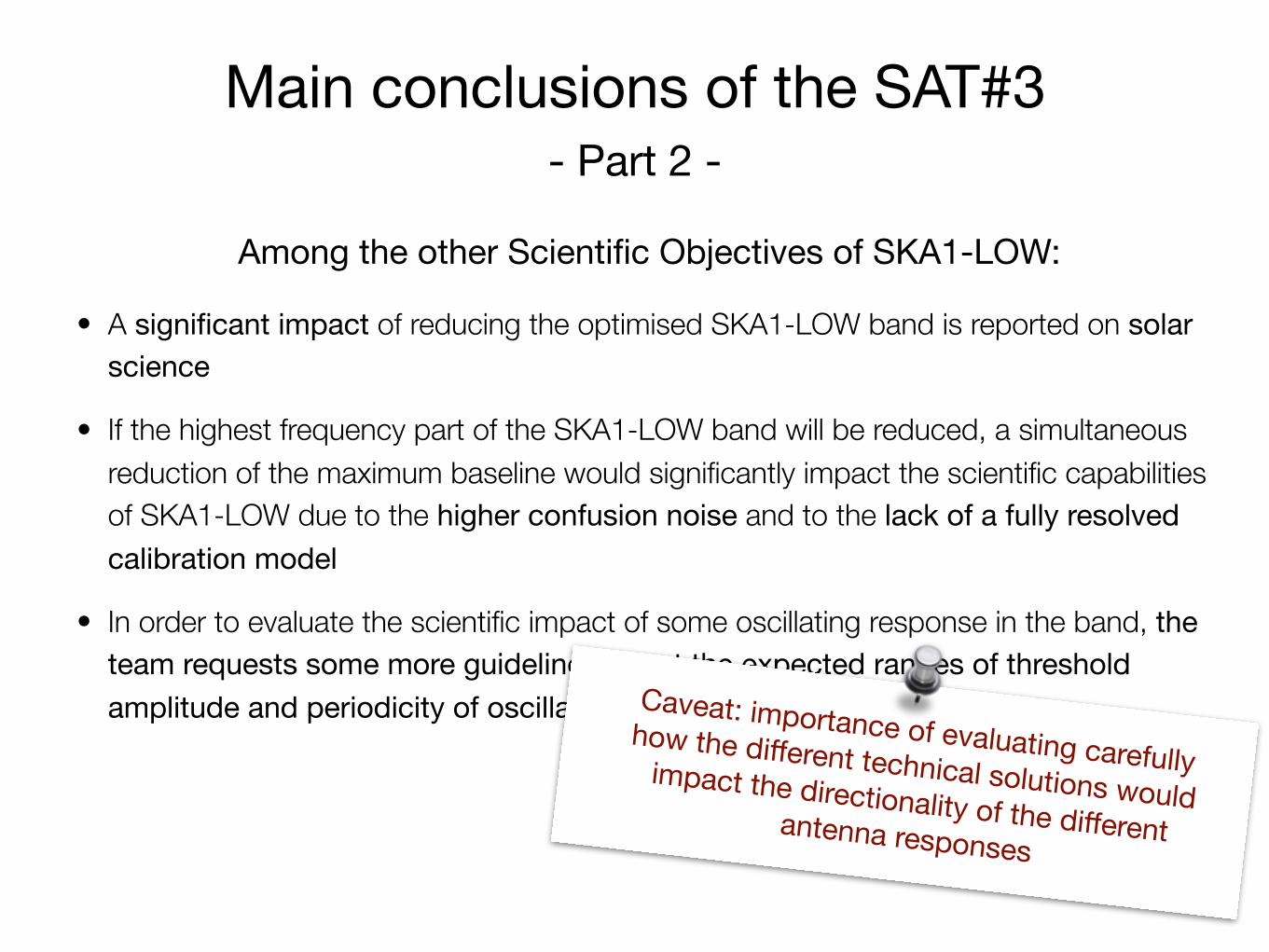
Main conclusions of the SAT#3- Part 2 -

Among the other Scientific Objectives of SKA1-LOW:

• A significant impact of reducing the optimised SKA1-LOW band is reported on solar science

• If the highest frequency part of the SKA1-LOW band will be reduced, a simultaneous reduction of the maximum baseline would significantly impact the scientific capabilities of SKA1-LOW due to the higher confusion noise and to the lack of a fully resolved calibration model

• In order to evaluate the scientific impact of some oscillating response in the band, the team requests some more guidelines about the expected ranges of threshold amplitude and periodicity of oscillation. Caveat: importance of evaluating carefully

how the different technical solutions would impact the directionality of the different antenna responses

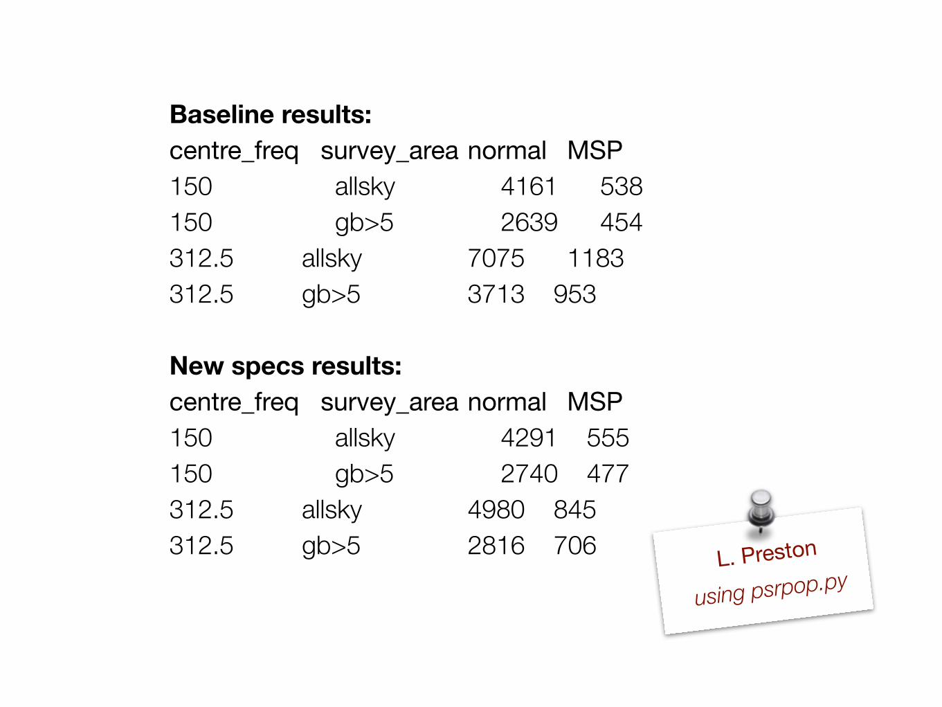
Baseline results: centre_freq survey_areanormal MSP150 allsky 4161 538 150 gb>5 2639 454 312.5 allsky 7075 1183 312.5 gb>5 3713 953

New specs results: centre_freq survey_areanormal MSP150 allsky 4291 555 150 gb>5 2740 477 312.5 allsky 4980 845 312.5 gb>5 2816 706 L. Preston

using psrpop.py

science assessment team #3 - ska indico (indico) · annalisa bonafede & chiara ferrari (with...

Documents