scheduling problem - optimization online · scheduling problem wagner emanoel costa ......

New VNS heuristic for Total Flowtime FlowshopScheduling Problem

Wagner Emanoel Costa Marco César GoldbargElizabeth G. Goldbarg

Technical Report - UFRN-DIMAp-2011-103-RT - Relatório TécnicoMarch - 2011 - Março

The contents of this document are the sole responsibility of the authors.O conteúdo do presente documento é de única responsabilidade dos autores.

Departamento de Informática e Matemática AplicadaUniversidade Federal do Rio Grande do Norte

www.dimap.ufrn.br

New VNS heuristic for Total Flowtime FlowshopScheduling Problem

Wagner Emanoel Costa ∗

[email protected]

Marco César Goldbarg †

[email protected]

Elizabeth G. Goldbarg ‡

[email protected]

Abstract. This paper develops a new VNS approach to Permutational Flow shop Sche-duling Problem with Total Flow time criterion. There are many hybrid approaches inthe problem’s literature, that make use of VNS internally, usually applying job insertneighbourhood followed by job interchange neighbourhood. In this study differentways to combine both neighbourhoods were examined. All tests use the benchmarkdata set from [18]. The results indicates, that there is a more profitable way to com-bine both neighbourhoods than the one frequently used in literature. The new VNSproduces results comparable with state-of-art methods, and obtained 25 novel soluti-ons.

Keywords: Flow-shop, Scheduling, Total Flow-time, Heuristics, VNS.

Resumo. Este documento desenvolve uma nova abordagem VNS para o problemaflow shop de permutação com critério total flow time. Existem muitas abordagenshíbridas, na literatura do problema, que utilizam algum tipo de VNS internamente,normalmente combinando as vizinhanças job insert e job interchange. Neste estudo,compara-se maneiras distintas de se combinar as duas vizinhanças. Todos os testesrealizados utilizam o conjunto de teste de [18]. Os resultados obtidos apontam parauma maneira mais proveitosa de se combinar as duas vizinhança tão comuns na li-teratudo do problema. A nova VNS produz resultados comparavéis com métodos doestado-da-arte, e encontrou 25 novas soluções.

Palavras-Chave: Flow-shop, Scheduling, Total Flow-time, Heuristics, VNS.

1 IntroductionIn permutational flow shop scheduling problem there is a set of jobs J = {1, 2, . . . , n}.

Each of n jobs has to be processed by a set of m machines M = {1, 2, . . . ,m}, sequentially

∗Programa de Pós-graduação em Sistemas e Computação, UFRN†Departamento de Informática e Matemática Aplicada - UFRN/CCET/DIMAp‡Departamento de Informática e Matemática Aplicada - UFRN/CCET/DIMAp

1

New VNS heuristic for Total Flowtime Flowshop Scheduling Problem 2

from the first machine to the last, in the same order. Each job j requires tjr units of time onmachine r. Each machine can process at most one job at any given time, and it can not be inter-rupted. Each job is available at time zero, and can be processed by at most one machine in anygiven time. Here the focus is to find the permutation of jobs Π = {π1, π2, . . . , πn}, such that thetotal completion time of jobs, named Total flow time (TFT ), is minimised. Equation 1 expressmathematically the concept of total flow time of a given permutation, Π, where C (πi,m) standsfor the completion time of job in position i of Π, πi.

TFT (Π) =n∑i=1

C (πi,m) (1)

The values of C (πi,m) can be evaluated using equations 2 to 5. Equations 2 and 3define the completion time relative to the first job in permutation Π, π1. Equation 2 definesthe completion time of the first job, π1, on the first machine as time required to complete itsprocessing, t1

1,1. It provides a base case for equation 3. Equation 3 defines the completiontime of π1 on machine r, 1 < r ≤ m, as the completion time of π1 on the previous machine,C(π1, r − 1), plus the processing time of job π1 on machine r, t1

1,r.

C (π1, 1) = tπ1,1 (2)

C (π1, r) = C (π1, r − 1) + tπ1,r ∀r ∈ {2, . . . ,m} (3)

Equations 4 and 5 evaluate the completion times for all jobs πi, 1 < i ≤ n. For the firstmachine, r = 1, C(πi, 1) is defined as the sum of the completion time of the previous job onthe first machine, C(πi−1, 1), with the processing time of πi, t1i,1. For all remaining machines,1 < r ≤ m, completion time of job πi, C(πi, r), 1 < i ≤ n, depends on two factors. First, thetime on which job πi will conclude its processing on the previous machine, r− 1, and thereforebecome available to be processed on machine r. Second, machine r can process job πi only, if rhas finished processing the previous job, πi−1. If machine r has not concluded the previous job,πi−1, than job πi will wait machine r conclusion of job πi−1. Equation 5 express both factors,and defines the completion time, C(πi, r), 1 < i ≤ n and 1 < r ≤ m, as the sum of processingtime t1i,r, with the greatest value between C(πi, r − 1) and C(πi−1, r).

C (πi, 1) = C (πi−1, 1) + tπi,1 ∀i ∈ {2, . . . , n} (4)

C (πi, r) =max {C (πi, r − 1) , C (πi−1, r)}+ tπi,r

∀i ∈ {2, . . . , n} ∀r ∈ {2, . . . ,m} (5)

Due to the fact, that the decision problem associated with TFT is NP-Complete in thestrong sense when m ≥ 2, [4], many heuristics approaches have been proposed to this problem.There are constructive methods such as [10, 3, 14, 15, 12], local search methods [10, 1], geneticalgorithms [13, 23, 21, 22], ant colonies [16, 24], particle swarm optimisation [19, 9, 8], beecolony optimization [20], hybrid discrete differential evolutionary algorithm [20], VNS andEDA-VNS [7].

From the cited approaches, the works of [23, 21, 7, 20, 22] are the ones which producedthe current state-of-art results.

A significant number of the state-of-art heuristics combines two neighbourhoods, namedjob insert and job interchange, in a internal VND procedure. The two neighbourhoods are


combined in the same order and in the same way in the works of [23, 7, 20, 22]. And so far nostudy has been reported, examining distinct combinations.

The present work exams different way to combine both neighbourhoods. The experimentsindicate, that a different combination from the one used in literature is more effective for theproblem. This new VNS approach is tested over all 120 instances of Taillard’s data set, [18],achieving 26 novel solutions.

The remaining of this paper is organised as follows. Section 2 reports a brief literaturereview of the problem. Section 3 describes the VNS approach, describes job insert and jobinterchange neighbourhoods and the different ways to combine both of them, and paramenterstested in the experiments. Section 4 reports the experiments to determine which combination ofneighbourhoods performs better, using a subset of instances from [18]. Section 5 describes thecomputational experiments and results obtained over all 120 instances of the data set. Section6 exposes the conclusions and future works.

2 Literature ReviewThis section reviews some methods proposed to PFSP with TFT criterion. Because the

literature of PFSP is extensive, this review is lmited to some constructive methods in literature,and meta-heuristic approaches that compose the current state-of-art of the problem.

The method of Rajendran and Ziegler [15] evaluates the lower bound for each job avai-lable to be assigned, m different solutions are created by changing how many machines areconsidered while evaluating the lower bound. For instance, the first solution is constructed bysorting the jobs, in non-decreasing order, by the weighted sum of processing times of all mmachines. The weights are defined in such way that one unit of processing time of a machine,r = j, has greater impact than one unit of time of subsequent machines, r > j. Equation 6shows the formula for the unweighted total flowtime. The equation for the weighted total flow-time is slightly different, but the weighted case is not the topic of this work. The processing timeof the first machine is removed, and the jobs re-sorted considering only the processing times ofthe m − 1 machines. This procedure is repeated, removing the data from one machine at eachiteration, until the last solution is created, when only the processing time of the last machineis taken into account. The best solution among the m created ones is then submitted to a localsearch procedure using job insert neighbourhood.

m∑r=j

(m− r + 1)Tri j ∈ {1, . . . ,m} (6)

The method H(1) presented in [10] weights down two criteria: weighted sum of machineidle time (IT ) and artificial flowtime (AT ). The idle time criterion for selecting job i when kjobs were already selected (ITik) is defined by Eq. (7), where wrk is calculated with Eq. (8).The term max {C(i, r − 1)− C(πk, r), 0} stands for the idle time of machine r. The weights,as defined on Eq. (8), stress that idle times on early machines are undesirable, for they delaythe remaining jobs. Such stress is stronger if there are many unscheduled jobs (small value ofk), and drops when the number k of scheduled jobs increases.

ITik =m∑r=2

wrkmax {C(i, r − 1)− C(πk, r), 0} (7)

wrk =m

r + k(m−r)n−2

(8)


The artificial flowtime (ATik) of candidate job i after k jobs were schedule refers to theTFT value obtained after including unscheduled job i, plus the time of an artificial job placedat the end of the sequence of jobs. The processing time of the artificial job on each machine isequal to the average processing time of all unscheduled jobs, excluding job i, on the correspon-dent machine.

Both criteria, ITik and ATik are combined according to Eq. (9).

fik = (n− k − 2)ITik + ATik (9)

Also, Liu and Reeves [10] propose a class of constructive heuristics named H(x), wherex is an integer, 1 ≤ x ≤ n. Each variant differs on the number of solutions it produces whichis given by x. While H(1) produces only one solution, H(2) produces 2 solutions and so on.These methods create new solutions by changing the initial job. Once the greedy criterion usedin these heuristics is adaptive, different initial jobs produce different solutions. H(1) uses thejob with the best value according to the greedy criterion as the initial job. H(2) creates twosolutions using each of the two best evaluated jobs as the initial job. Thus, the first solutiongenerated by H(2) is exactly the same one produce by H(1). The second solution uses thesecond best job as the initial one. A special case is H( n

10) which uses the same principle,

producing n10

solutions with the best n10

initial jobs. The work of [10] also proposes the use ofjob interchange local search to further improve the greedy solution obtained.

Framinan et al. [3] define a queue based on the sum of the processing times of eachjob. The job on top of the queue is inserted in the best possible position in the partial solution.Later the inserted job can be interchanged with any other job in the partial solution in order tominimise the current value of the total flowtime. Nagano and Moccellin [12] create the queue inthe same way as in [2]. The algorithm iteratively removes the first job in the queue and placesit at the end of the partial solution. Local search methods, job insert and interchange, are thenapplied over the partial sequence to minimise total flowtime.

The iterated local search proposed by Dong et al. [1] adopts the job at index neigh-bourhood created by [16]. This neighbourhood consists of job insert moves; the order in whichneighbours solutions are created is dependant of the best solution found so far. In Dong et al.[1] each time the local search procedure gets trapped in local optima, a perturbation over the so-lution is performed and local search resumed. In this case the perturbation consists of randomlyinterchanging six adjacent jobs in the solution.

The hybrid genetic algorithm of Zhang et al. [23] applies a data mining procedure overits population, creating a table that maps jobs to positions and counts how many “good” so-lutions have a given association job/position. An assignment procedure creates a solution thatwill be used during crossover operations to preserve building blocks in the new solutions. So-lutions obtained after crossover are submitted to local searches (with job insert and interchangeneighbourhoods). The hybrid genetic with local search of Tseng and Lin [21] uses an ortho-gonal crossover operator to recombine solutions. New solutions are submitted to two localsearches that use the job insert neighbourhood. One local search method is driven to minimiseTFT while the other looks for minimising idle times. The latter is used to escape local optimaachieved by the former and then minimisation of TFT is resumed. The asynchronous geneticalgorithm, AGA, of [22], has a population of 40 solutions, one of them generated using H

(nm

)heuristic, where n

mare created using the H criterion, followed by interchange local search , the

other 39 are randomly generated. Each iteration the evolution process submit solution to E-VNS(an specific VNS approach), crossover and E-VNS a second time. If all individual in populationhave the same TFT value, the population is restarted, by random generating 38 individuals,keeping the best solution in the current pool of solutions and inserting the solution generated


by LR(nm

)again. The E-VNS uses job insert local search and job interchange. When using

job insert local search, a job πi is randomly selected. E-VNS will attempt to re-insert πi ona different position j, also randomly selected. If such attempt improves current solution, thenew solution is accepted and a new iteration of job insert occurs, selecting another random jobto be re-inserted. E-VNS execute 50 iterations of job insert. After them, 50 iterations of jobinterchange occurs, where the jobs to be interchange are randomly selected, if any improvementis achieved the solution is accepted and E-VNS resumes job insert local search. The number oftimes job insert can be resumed is limited by a value, randomly selected each time E-VNS iscalled, between 10 and 60, therefore is possible to E-VNS to terminate not trapped in a localoptimum. AGA uses a two point crossover defined in [11]. The pair of parents used in crossoverare randomly selected. The crossover chooses two random points, s and t, of a parent, the blockof jobs within the index (πi, s ≤ i ≤ t) are copied to their respective positions in a new solution,the remaining positions are filled following the job order on the second parent. Such crossoveris applied twice for each pair of parents creating 2 new solutions. Each iteration applies thecrossover operator repeatedly, until 40 new solutions are created, replacing the previous popu-lation. E-VNS is applied over the new solutions. AGA stops if a time limit of 0.4 × n × mseconds is achieved.

Rajendran and Ziegler [16] propose two ant colonies for the problem, they are namedMMAS and PACO. Both of them apply three iterations of job at index local search once a solu-tion has been fully constructed. MMAS and PACO differ on how the probabilities are assignedto unscheduled jobs while constructing the solution. MMAS adopts uniform distribution for thebest five options, while PACO gives distinct probabilities to the five best options. The ant colonynamed SACO [24] starts using uniform probability distribution and evolves the probabilities ofthe pheromones using Kullback-Liebler divergence (see [24] for further details).

The PSO of Tasgetiren et al. [19] uses a real representation of solution and a rule is used todecode the real representation into a permutational representation. The particles move towardsthe best global point and the best previous position visited. A variable neighbourhood descent(VND) approach (using interchange and job insert neighbourhoods) is defined and applied to thebest solution in the population each generation. The PSO of Liao et al. [9] represents a solutionusing a discrete binary matrix B, where job i is assigned to position j if the entry bij = 1.The velocity represents probabilities of changes within B. This PSO uses two local searches(interchange and job insert) but limits the neighbourhood size. Depending on the jobs positions,the search procedure considers only movements within a distance of 12 positions (e.g. a job inthe first position cannot be inserted in position 14 or further, neither can it be interchanged withanother job placed in position 14 or above). The PSO of Jarboui et al. [8] uses the permutationrepresentation and applies a simulated annealing method to optimise solutions whose TFT iswithin 2% of the best TFT value obtained up so far.

The VNS of Jarboui et al. [7] uses two neighbourhoods: job insert and interchange. Itstarts using job insert. Once this neighbourhood cannot improve the current solution, the proce-dure migrates to interchange neighbourhood and keeps using interchange moves until no impro-vement can be reached, when it reverts to using job insert. If both neighbourhoods fail to furtherimprove a solution, this VNS makes a copy of the best solution found, applies over it a randominterchange move, and resumes optimisation using job insert neighbourhood. The algorithmalternates between the two neighbourhoods until both of them are not able to produce improve-ments on the current solution. At this point, the algorithm applies a random interchange moveon the best solution found so far and resumes optimisation with the job insert neighbourhood.

EDA-VNS [7] is a hybrid evolutionary approach. It uses a population of 10 solutionswhere a subset Q of three solutions is selected. A probabilistic model is constructed based on


Q which is used to generate new solutions. If a new solution is better than the worst solutionin the population, the new one replaces the worst solution. There is a probability to apply VNSover a solution. Such probability is related to objective function, the closer the value is to thebest found fow-time value the better are the chances that VNS will be applied over a solution.The closer the value of a given solution is to the best flowtime value found so far, the better thechances of VNS is applied to that solution. The chances drop exponentially for farther valuesto a minimum of 1%.

Tasgetiren et al. [20] propose two approaches for TFT : a bee colony optimisation (namedDABC) and a hybrid evolutionary approach (hDDE). There is a population of ten bees in DABC,each one executing one of three activities. In the first activity, named employed bee phase,the bee exploits its current solution by randomly choosing between three methods: job insert,interchange or iterated greedy neighbourhood [17]. Once a neighbour is chosen, it is furtherimproved using VNS. In the second activity, named onlooker phase, the bee migrates to anothersolution, randomly picking two solutions from the other bees and keeping the better one. Then,the bee creates a neighbour of the chosen solution, using the same schemes from employed bee,and applies the VNS of Jarboui et al. [7] afterwards. In the third activity, named scout, the beegenerates two random solutions, keeps the worst one and applies the iterated greedy move overit. The algorithm hDDE also uses a population with 10 individuals. Its solution representationis discrete. Mutation is done by a random insert or interchange move. The crossover operatortakes a muted individual and combines it with a non-mutated solution. For a given position pos,the crossover picks a random number c within [0, 1]. If c is smaller than a constant CR = 0.9,the value from the mutated solution fills position pos, otherwise the value for pos comes fromthe non-mutated one. There is a probability of 1% of applying VNS (insert and interchangemoves only) over an individual. The iterated greedy procedure is applied only over the bestindividual of the population. Crossover and mutation rates are 90% and 20%, respectively.

The results produced by AGA [22], DABC, hDDE [20], VNS, EDA-VNS [7], HGA [23]and HGLS [21] are used as references for the experiments presented here, once these methods,present the best results over Flowshop instances created by Taillard [18], as far as the authors’knowledge concerns. These instances have been used as test set for flowshop TFT and areused here on the computational experiments to assess the proposed approach performance incomparison to the state-of-art methods.

3 Variable Neighbourhood Search - VNSVNS is a metaheuristic approach proposed in 1997 by Hansen & Mladenovic for the p-

median problem, [5]. In a recent review of VNS [6], the creators of VNS define it as “. . . ametaheuristic which systematically exploits the idea of neighbourhood change, both in descentto local minima and in escape from the valleys which contain them”.

Because of its simplicity and efficiency, VNS is often hybridised with other heuristics inorder to achieve solutions of higher quality. VNS have few parameters, at the same time, it hasa historic of good results in many problems including flowshop. The approaches presented by[7], VNS and EDA-VNS, are examples of how VNS can be effective by itself or hybridisedwith an evolutionary approach.

In order to implement VNS the parameters to be defined in a VNS are:

1. A initial solution.

2. A perturbation scheme, named Shake procedure, used to escape local optimum commonto multiple neighbourhoods;


3. A set of local searches neighbourhoods;

4. A scheme to define when to change the neighbourhood.

The first two items are simple to solve. An initial solution can be generated randomlyor using greedy procedure. The work of [1] tested many greedy heuristic as source for initialsolution for its local search methods, when compaed with other greedy approaches. Their ex-periments conclude that H heuristics proposed by [10] produced better results. Therefore Hmethods are tested in section 4. The second item, Shake, can be easily implemented usingrandom moves from a given neighbourhood,as suggested in [6]. This parameter is also tested insection 4. The remaining of this section is devoted to items 3 and 4, describing neighbourhoodsand VNS approaches tested.

Considering the particular case of permutational flow shop with TFT criterion, two localsearches methods are repeatedly used in literature. They are job insert local search, also referredas shift local search, and the job interchange local search, [23, 7, 20, 22]. The neighbourhoodstructures used in these local search are explained next.

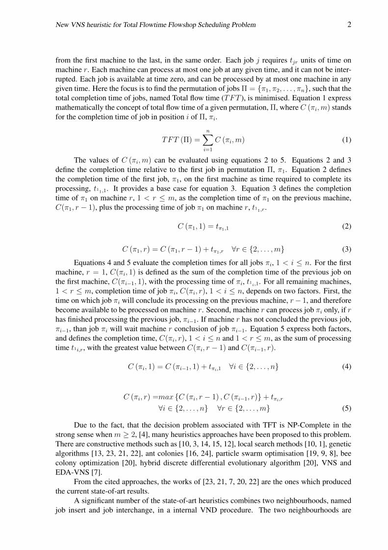
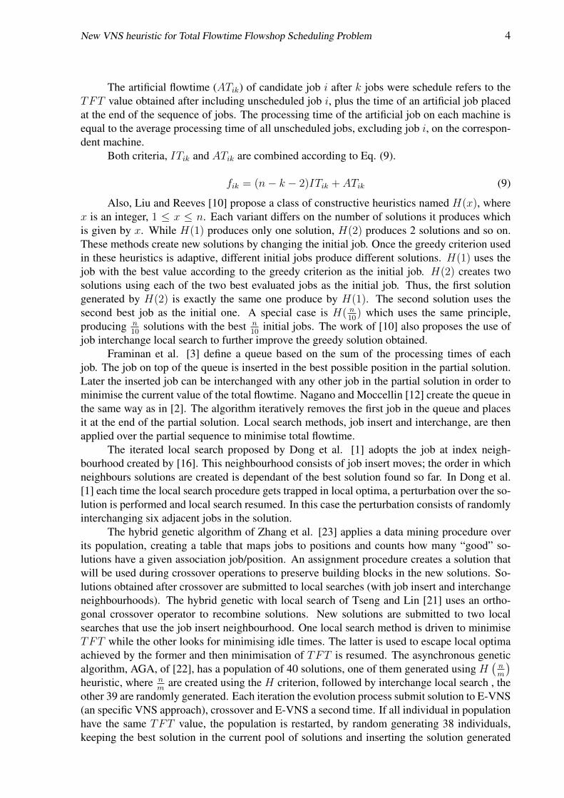
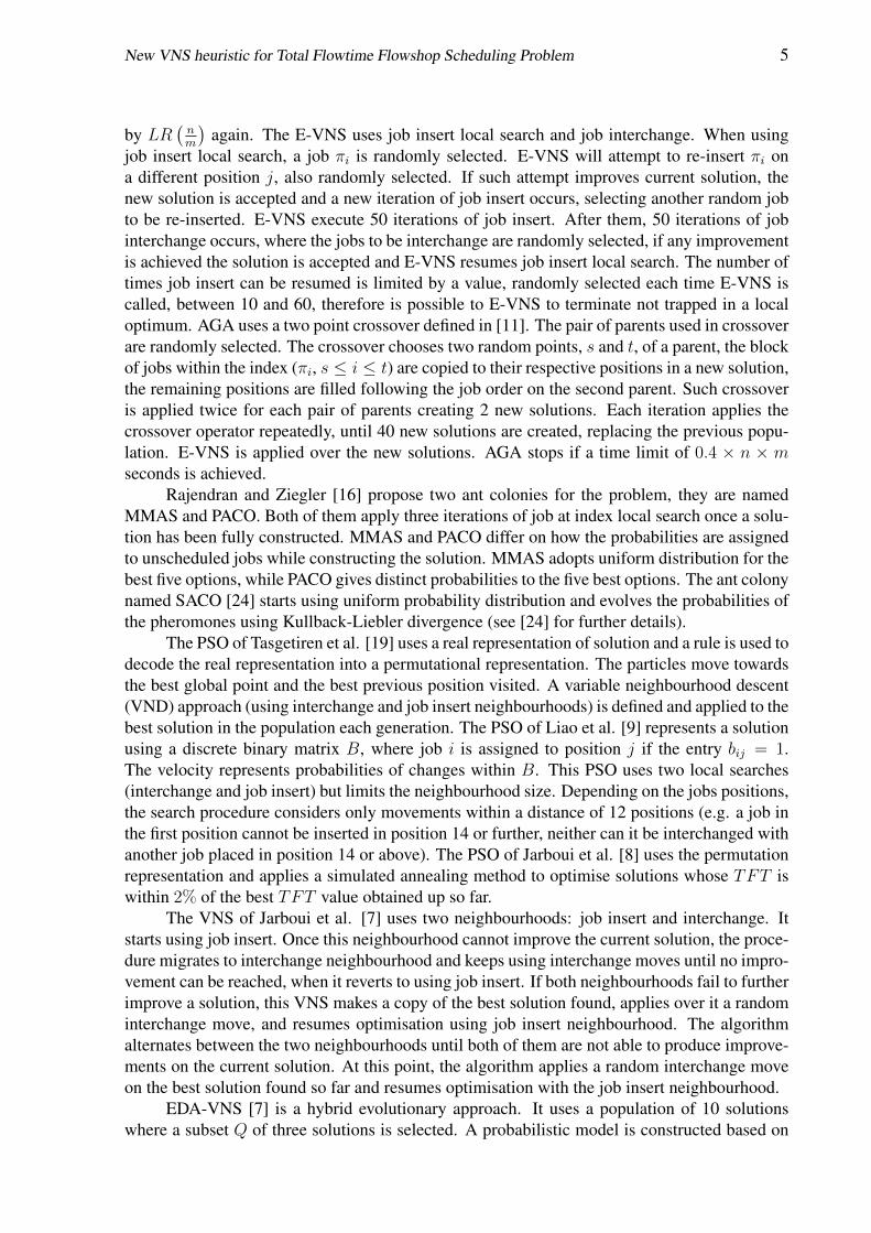
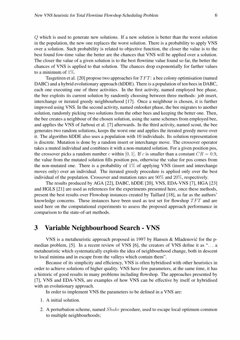
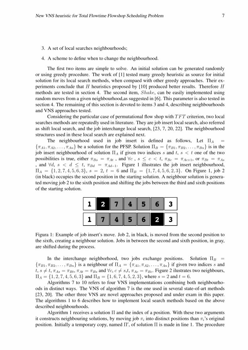
The neighbourhood used in job insert is defined as follows, Let ΠA ={πA1, πA2, . . . , πAn} be a solution for the PFSP. Solution ΠB = {πB1, πB2, . . . , πBn} is in thejob insert neighbourhood of solution ΠA if given two indices s and t, s < t one of the twopossibilities is true, either πBs = πAt , and ∀c , s ≤ c < t, πBc = πAc+1, or πBt = πAs, and ∀d, s < d ≤ t, πBd = πAd−1. Figure 1 illustrates the job insert neighbourhood,ΠA = {1, 2, 7, 4, 5, 6, 3}, s = 2, t = 6 and ΠB = {1, 7, 4, 5, 6, 2, 3}. On Figure 1, job 2(in black) occupies the second position in the starting solution. A neighbour solution is genera-ted moving job 2 to the sixth position and shifting the jobs between the third and sixth positionsof the starting solution.

Figura 1: Example of job insert’s move. Job 2, in black, is moved from the second position tothe sixth, creating a neighbour solution. Jobs in between the second and sixth position, in gray,are shifted during the process.

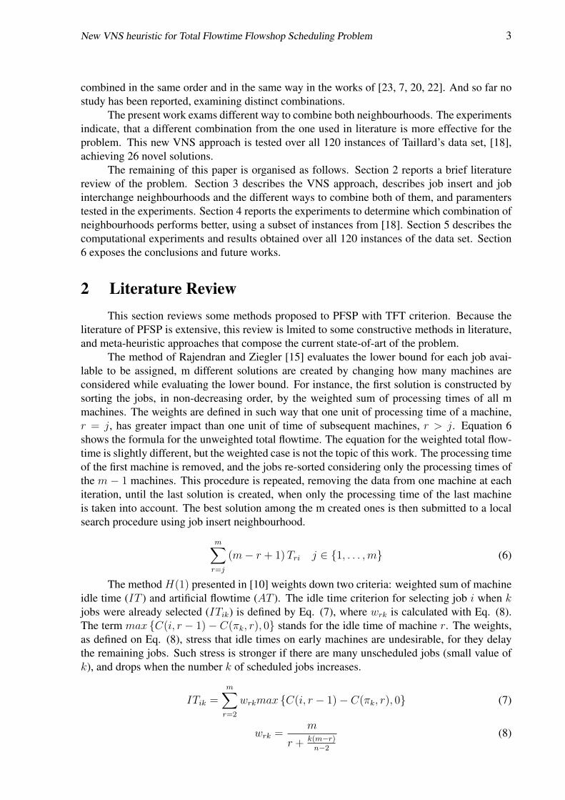
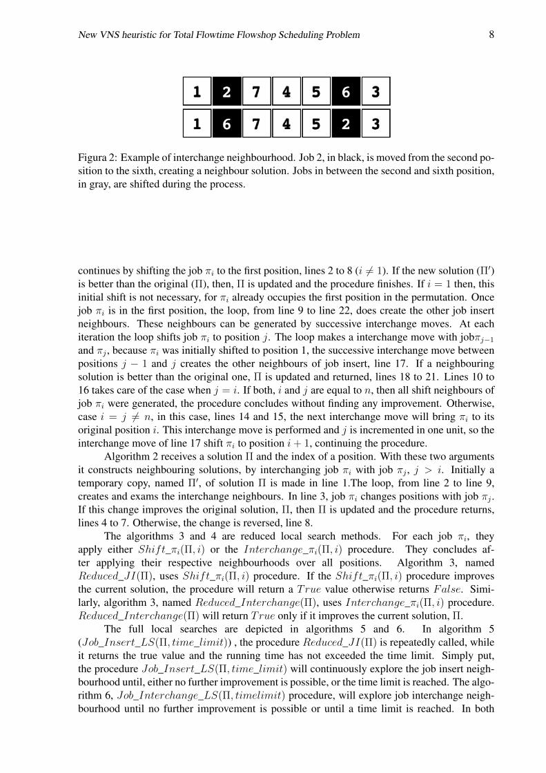
In the interchange neighborhood, two jobs exchange positions. Solution ΠB ={πB1, πB2, . . . , πBn} is a neighbour of ΠA = {πA1, πA2, . . . , πAn} if given two indices s andt, s 6= t, πAs = πBt, πAt = πBs and ∀c, c 6= s,t, πAc = πBc. Figure 2 ilustrates two neighbours,ΠA = {1, 2, 7, 4, 5, 6, 3} and ΠB = {1, 6, 7, 4, 5, 2, 3}, where s = 2 and t = 6.

Algorithms 7 to 10 refers to four VNS implementations combining both neighbourho-ods in distinct ways. The VNS of algorithm 7 is the one used in several state-of-art methods[23, 20]. The other three VNS are novel approaches proposed and under exam in this paper.The algorithms 1 to 6 describes how to implement local search methods based on the abovedescribed neighbourhoods.

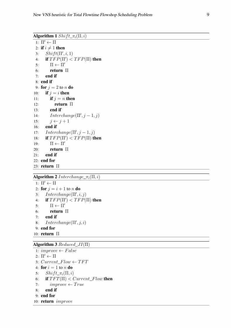
Algorithm 1 receives a solution Π and the index of a position. With these two argumentsit constructs neighbouring solutions, by moving job πi into distinct positions than πi’s originalposition. Initially a temporary copy, named Π′, of solution Π is made in line 1. The procedure


Figura 2: Example of interchange neighbourhood. Job 2, in black, is moved from the second po-sition to the sixth, creating a neighbour solution. Jobs in between the second and sixth position,in gray, are shifted during the process.

continues by shifting the job πi to the first position, lines 2 to 8 (i 6= 1). If the new solution (Π′)is better than the original (Π), then, Π is updated and the procedure finishes. If i = 1 then, thisinitial shift is not necessary, for πi already occupies the first position in the permutation. Oncejob πi is in the first position, the loop, from line 9 to line 22, does create the other job insertneighbours. These neighbours can be generated by successive interchange moves. At eachiteration the loop shifts job πi to position j. The loop makes a interchange move with jobπj−1and πj , because πi was initially shifted to position 1, the successive interchange move betweenpositions j − 1 and j creates the other neighbours of job insert, line 17. If a neighbouringsolution is better than the original one, Π is updated and returned, lines 18 to 21. Lines 10 to16 takes care of the case when j = i. If both, i and j are equal to n, then all shift neighbours ofjob πi were generated, the procedure concludes without finding any improvement. Otherwise,case i = j 6= n, in this case, lines 14 and 15, the next interchange move will bring πi to itsoriginal position i. This interchange move is performed and j is incremented in one unit, so theinterchange move of line 17 shift πi to position i+ 1, continuing the procedure.

Algorithm 2 receives a solution Π and the index of a position. With these two argumentsit constructs neighbouring solutions, by interchanging job πi with job πj , j > i. Initially atemporary copy, named Π′, of solution Π is made in line 1.The loop, from line 2 to line 9,creates and exams the interchange neighbours. In line 3, job πi changes positions with job πj .If this change improves the original solution, Π, then Π is updated and the procedure returns,lines 4 to 7. Otherwise, the change is reversed, line 8.

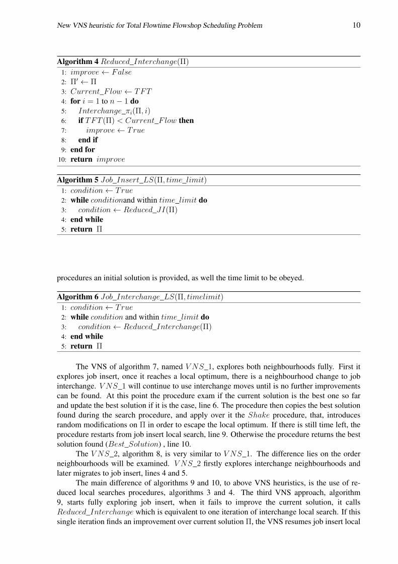
The algorithms 3 and 4 are reduced local search methods. For each job πi, theyapply either Shift_πi(Π, i) or the Interchange_πi(Π, i) procedure. They concludes af-ter applying their respective neighbourhoods over all positions. Algorithm 3, namedReduced_JI(Π), uses Shift_πi(Π, i) procedure. If the Shift_πi(Π, i) procedure improvesthe current solution, the procedure will return a True value otherwise returns False. Simi-larly, algorithm 3, named Reduced_Interchange(Π), uses Interchange_πi(Π, i) procedure.Reduced_Interchange(Π) will return True only if it improves the current solution, Π.

The full local searches are depicted in algorithms 5 and 6. In algorithm 5(Job_Insert_LS(Π, time_limit)) , the procedure Reduced_JI(Π) is repeatedly called, whileit returns the true value and the running time has not exceeded the time limit. Simply put,the procedure Job_Insert_LS(Π, time_limit) will continuously explore the job insert neigh-bourhood until, either no further improvement is possible, or the time limit is reached. The algo-rithm 6, Job_Interchange_LS(Π, timelimit) procedure, will explore job interchange neigh-bourhood until no further improvement is possible or until a time limit is reached. In both


Algorithm 1 Shift_πi(Π, i)1: Π′ ← Π2: if i 6= 1 then3: Shift(Π′, i, 1)4: if TFP (Π′) < TFP (Π) then5: Π← Π′

6: return Π7: end if8: end if9: for j = 2 to n do

10: if j = i then11: if j = n then12: return Π13: end if14: Interchange(Π′, j − 1, j)15: j ← j + 116: end if17: Interchange(Π′, j − 1, j)18: if TFP (Π′) < TFP (Π) then19: Π← Π′

20: return Π21: end if22: end for23: return Π

Algorithm 2 Interchange_πi(Π, i)1: Π′ ← Π2: for j = i+ 1 to n do3: Interchange(Π′, i, j)4: if TFP (Π′) < TFP (Π) then5: Π← Π′

6: return Π7: end if8: Interchange(Π′, j, i)9: end for

10: return Π

Algorithm 3 Reduced_JI(Π)

1: improve← False2: Π′ ← Π3: Current_Flow ← TFT4: for i = 1 to n do5: Shift_πi(Π, i)6: if TFT (Π) < Current_Flow then7: improve← True8: end if9: end for

10: return improve


Algorithm 4 Reduced_Interchange(Π)

1: improve← False2: Π′ ← Π3: Current_Flow ← TFT4: for i = 1 to n− 1 do5: Interchange_πi(Π, i)6: if TFT (Π) < Current_Flow then7: improve← True8: end if9: end for

10: return improve

Algorithm 5 Job_Insert_LS(Π, time_limit)1: condition← True2: while conditionand within time_limit do3: condition← Reduced_JI(Π)4: end while5: return Π

procedures an initial solution is provided, as well the time limit to be obeyed.

Algorithm 6 Job_Interchange_LS(Π, timelimit)

1: condition← True2: while condition and within time_limit do3: condition← Reduced_Interchange(Π)4: end while5: return Π

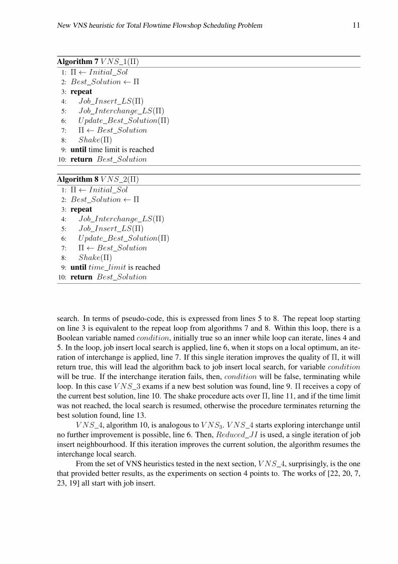
The VNS of algorithm 7, named V NS_1, explores both neighbourhoods fully. First itexplores job insert, once it reaches a local optimum, there is a neighbourhood change to jobinterchange. V NS_1 will continue to use interchange moves until is no further improvementscan be found. At this point the procedure exam if the current solution is the best one so farand update the best solution if it is the case, line 6. The procedure then copies the best solutionfound during the search procedure, and apply over it the Shake procedure, that, introducesrandom modifications on Π in order to escape the local optimum. If there is still time left, theprocedure restarts from job insert local search, line 9. Otherwise the procedure returns the bestsolution found (Best_Solution) , line 10.

The V NS_2, algorithm 8, is very similar to V NS_1. The difference lies on the orderneighbourhoods will be examined. V NS_2 firstly explores interchange neighbourhoods andlater migrates to job insert, lines 4 and 5.

The main difference of algorithms 9 and 10, to above VNS heuristics, is the use of re-duced local searches procedures, algorithms 3 and 4. The third VNS approach, algorithm9, starts fully exploring job insert, when it fails to improve the current solution, it callsReduced_Interchange which is equivalent to one iteration of interchange local search. If thissingle iteration finds an improvement over current solution Π, the VNS resumes job insert local


Algorithm 7 V NS_1(Π)

1: Π← Initial_Sol2: Best_Solution← Π3: repeat4: Job_Insert_LS(Π)5: Job_Interchange_LS(Π)6: Update_Best_Solution(Π)7: Π← Best_Solution8: Shake(Π)9: until time limit is reached

10: return Best_Solution

Algorithm 8 V NS_2(Π)

1: Π← Initial_Sol2: Best_Solution← Π3: repeat4: Job_Interchange_LS(Π)5: Job_Insert_LS(Π)6: Update_Best_Solution(Π)7: Π← Best_Solution8: Shake(Π)9: until time_limit is reached

10: return Best_Solution

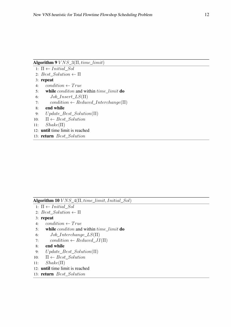
search. In terms of pseudo-code, this is expressed from lines 5 to 8. The repeat loop startingon line 3 is equivalent to the repeat loop from algorithms 7 and 8. Within this loop, there is aBoolean variable named condition, initially true so an inner while loop can iterate, lines 4 and5. In the loop, job insert local search is applied, line 6, when it stops on a local optimum, an ite-ration of interchange is applied, line 7. If this single iteration improves the quality of Π, it willreturn true, this will lead the algorithm back to job insert local search, for variable conditionwill be true. If the interchange iteration fails, then, condition will be false, terminating whileloop. In this case V NS_3 exams if a new best solution was found, line 9. Π receives a copy ofthe current best solution, line 10. The shake procedure acts over Π, line 11, and if the time limitwas not reached, the local search is resumed, otherwise the procedure terminates returning thebest solution found, line 13.

V NS_4, algorithm 10, is analogous to V NS3. V NS_4 starts exploring interchange untilno further improvement is possible, line 6. Then, Reduced_JI is used, a single iteration of jobinsert neighbourhood. If this iteration improves the current solution, the algorithm resumes theinterchange local search.

From the set of VNS heuristics tested in the next section, V NS_4, surprisingly, is the onethat provided better results, as the experiments on section 4 points to. The works of [22, 20, 7,23, 19] all start with job insert.


Algorithm 9 V NS_3(Π, time_limit)1: Π← Initial_Sol2: Best_Solution← Π3: repeat4: condition← True5: while conditon and within time_limit do6: Job_Insert_LS(Π)7: condition← Reduced_Interchange(Π)8: end while9: Update_Best_Solution(Π)

10: Π← Best_Solution11: Shake(Π)12: until time limit is reached13: return Best_Solution

Algorithm 10 V NS_4(Π, time_limit, Initial_Sol)1: Π← Initial_Sol2: Best_Solution← Π3: repeat4: condition← True5: while conditon and within time_limit do6: Job_Interchange_LS(Π)7: condition← Reduced_JI(Π)8: end while9: Update_Best_Solution(Π)

10: Π← Best_Solution11: Shake(Π)12: until time limit is reached13: return Best_Solution


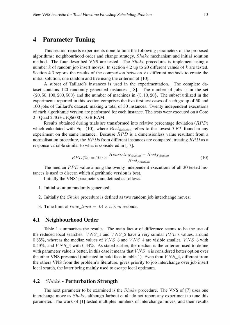
4 Parameter TuningThis section reports experiments done to tune the following parameters of the proposed

algorithms: neighbourhood order and change strategy, Shake mechanism and initial solutionmethod. The four described VNS are tested. The Shake procedures is implement using anumber k of random job insert moves. In section 4.2 up to 20 different values of k are tested.Section 4.3 reports the results of the comparison between six different methods to create theinitial solution, one random and five using the criterion of [10].

A subset of Taillard’s instances is used in the experimentation. The complete da-taset contains 120 randomly generated instances [18]. The number of jobs is in the set{20, 50, 100, 200, 500} and the number of machines in {5, 10, 20}. The subset utilized in theexperiments reported in this section comprises the five first test cases of each group of 50 and100 jobs of Taillard’s dataset, making a total of 30 instances. Twenty independent executionsof each algorithmic version are performed for each instance. The tests were executed on a Core2 - Quad 2.4GHz (Q6600), 1GB RAM.

Results obtained during trials are transformed into relative percentage deviation (RPD)which calculated with Eq. (10), where BestSolution refers to the lowest TFT found in anyexperiment on the same instance. Because RPD is a dimensionless value resultant from anormalisation procedure, the RPDs from different instances are compared, treating RPD as aresponse variable similar to what is considered in [17].

RPD(%) = 100× HeuristicSolution −BestSolutionBestSolution

(10)

The median RPD value among the twenty independent executions of all 30 tested ins-tances is used to discern which algorithmic version is best.

Initially the VNS’ parameters are defined as follows:

1. Initial solution randomly generated;

2. Initially the Shake procedure is defined as two random job interchange moves;

3. Time limit of time_limit = 0.4× n×m seconds.

4.1 Neighbourhood OrderTable 1 summarises the results. The main factor of difference seems to be the use of

the reduced local searches. V NS_1 and V NS_2 have a very similar RPD’s values, around0.65%, whereas the median values of V NS_3 and V NS_4 are visible smaller. V NS_3 with0.49%, and V NS_4 with 0.44%. As stated earlier, the median is the criterion used to definewith parameter value is better, in this case it means that V NS_4 is considered better option overthe other VNS presented (indicated in bold face in table 1). Even thou V NS_4, different fromthe others VNS from the problem’s literature, gives priority to job interchange over job insertlocal search, the latter being mainly used to escape local optimum.

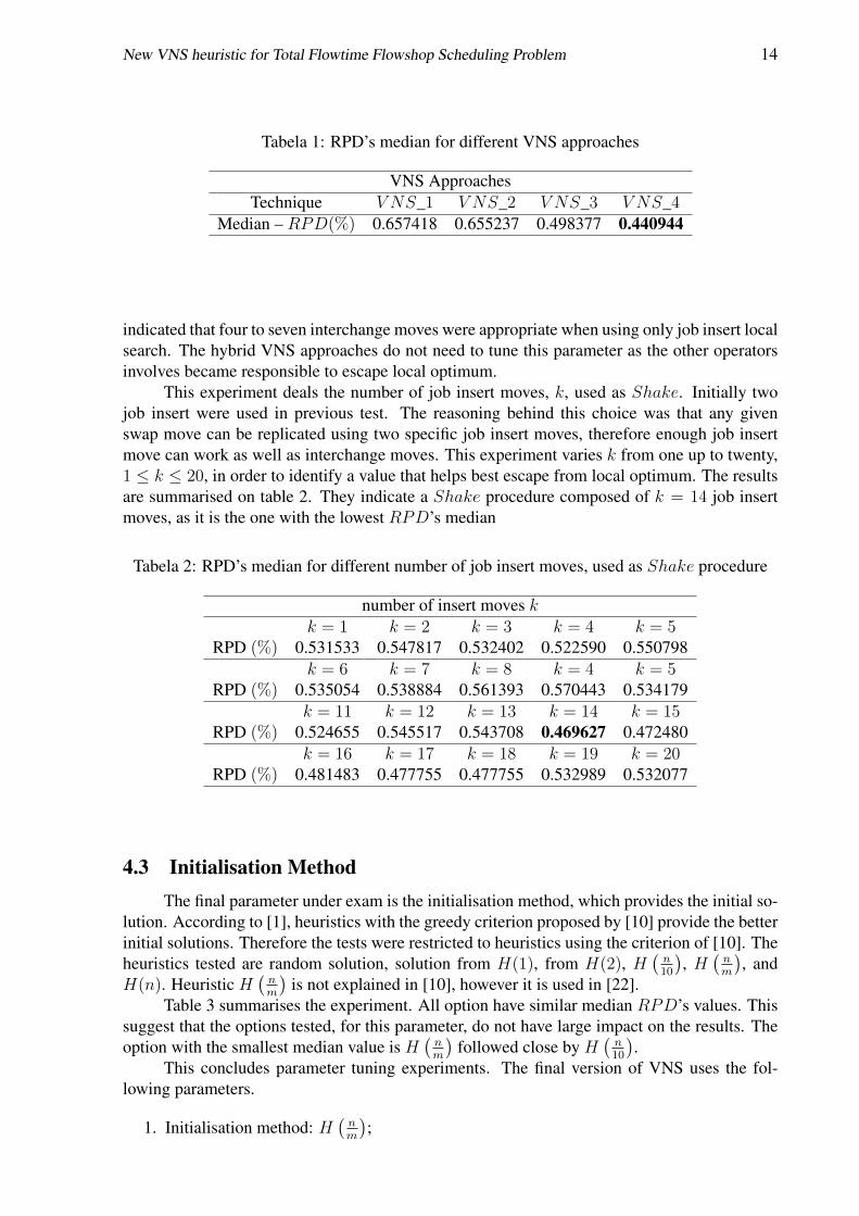
4.2 Shake - Perturbation StrengthThe next parameter to be examined is the Shake procedure. The VNS of [7] uses one

interchange move as Shake, although Jarboui et al. do not report any experiment to tune thisparameter. The work of [1] tested multiples numbers of interchange moves, and their results


Tabela 1: RPD’s median for different VNS approaches

VNS ApproachesTechnique V NS_1 V NS_2 V NS_3 V NS_4

Median – RPD(%) 0.657418 0.655237 0.498377 0.440944

indicated that four to seven interchange moves were appropriate when using only job insert localsearch. The hybrid VNS approaches do not need to tune this parameter as the other operatorsinvolves became responsible to escape local optimum.

This experiment deals the number of job insert moves, k, used as Shake. Initially twojob insert were used in previous test. The reasoning behind this choice was that any givenswap move can be replicated using two specific job insert moves, therefore enough job insertmove can work as well as interchange moves. This experiment varies k from one up to twenty,1 ≤ k ≤ 20, in order to identify a value that helps best escape from local optimum. The resultsare summarised on table 2. They indicate a Shake procedure composed of k = 14 job insertmoves, as it is the one with the lowest RPD’s median

Tabela 2: RPD’s median for different number of job insert moves, used as Shake procedure

number of insert moves kk = 1 k = 2 k = 3 k = 4 k = 5

RPD (%) 0.531533 0.547817 0.532402 0.522590 0.550798k = 6 k = 7 k = 8 k = 4 k = 5

RPD (%) 0.535054 0.538884 0.561393 0.570443 0.534179k = 11 k = 12 k = 13 k = 14 k = 15

RPD (%) 0.524655 0.545517 0.543708 0.469627 0.472480k = 16 k = 17 k = 18 k = 19 k = 20

RPD (%) 0.481483 0.477755 0.477755 0.532989 0.532077

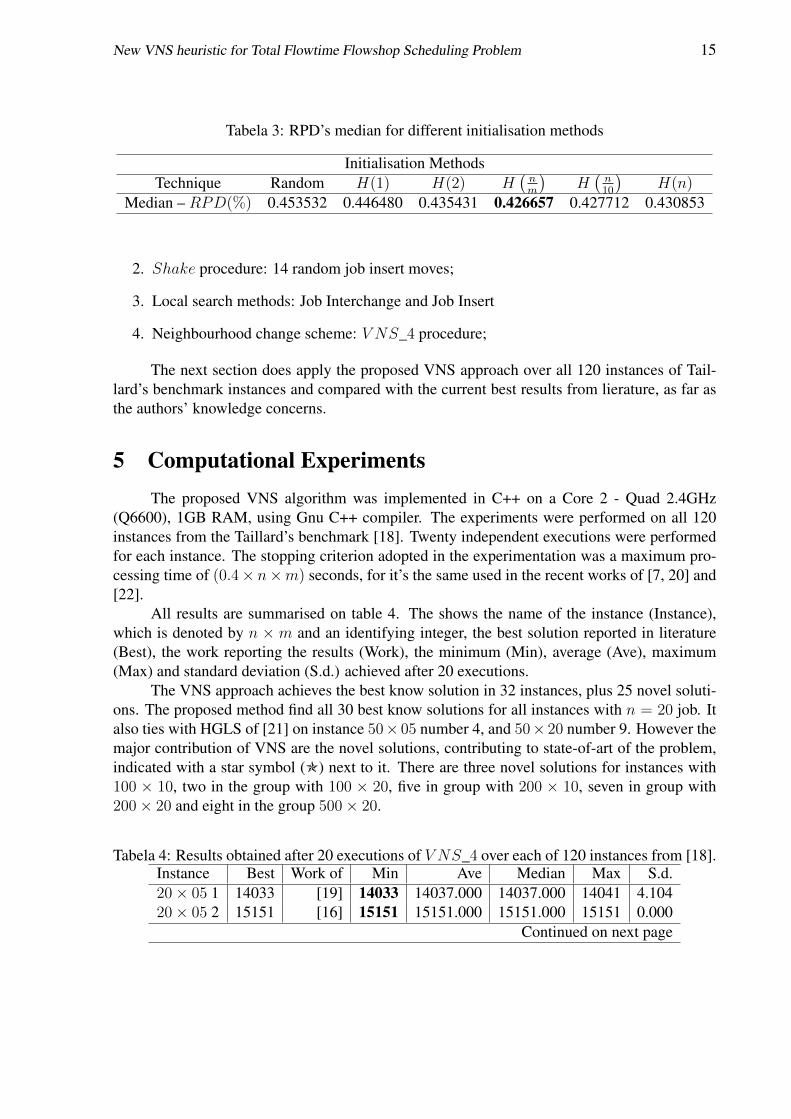
4.3 Initialisation MethodThe final parameter under exam is the initialisation method, which provides the initial so-

lution. According to [1], heuristics with the greedy criterion proposed by [10] provide the betterinitial solutions. Therefore the tests were restricted to heuristics using the criterion of [10]. Theheuristics tested are random solution, solution from H(1), from H(2), H

(n10

), H

(nm

), and

H(n). Heuristic H(nm

)is not explained in [10], however it is used in [22].

Table 3 summarises the experiment. All option have similar median RPD’s values. Thissuggest that the options tested, for this parameter, do not have large impact on the results. Theoption with the smallest median value is H

(nm

)followed close by H

(n10

).

This concludes parameter tuning experiments. The final version of VNS uses the fol-lowing parameters.

1. Initialisation method: H(nm

);


Tabela 3: RPD’s median for different initialisation methods

Initialisation MethodsTechnique Random H(1) H(2) H

(nm

)H(n10

)H(n)

Median – RPD(%) 0.453532 0.446480 0.435431 0.426657 0.427712 0.430853

2. Shake procedure: 14 random job insert moves;

3. Local search methods: Job Interchange and Job Insert

4. Neighbourhood change scheme: V NS_4 procedure;

The next section does apply the proposed VNS approach over all 120 instances of Tail-lard’s benchmark instances and compared with the current best results from lierature, as far asthe authors’ knowledge concerns.

5 Computational ExperimentsThe proposed VNS algorithm was implemented in C++ on a Core 2 - Quad 2.4GHz

(Q6600), 1GB RAM, using Gnu C++ compiler. The experiments were performed on all 120instances from the Taillard’s benchmark [18]. Twenty independent executions were performedfor each instance. The stopping criterion adopted in the experimentation was a maximum pro-cessing time of (0.4× n×m) seconds, for it’s the same used in the recent works of [7, 20] and[22].

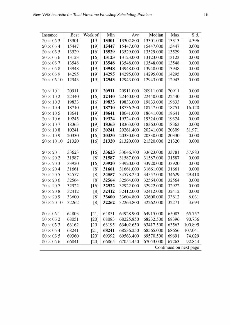
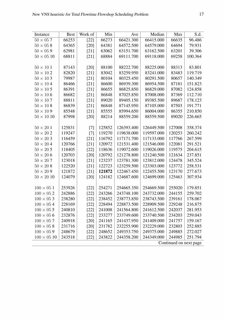
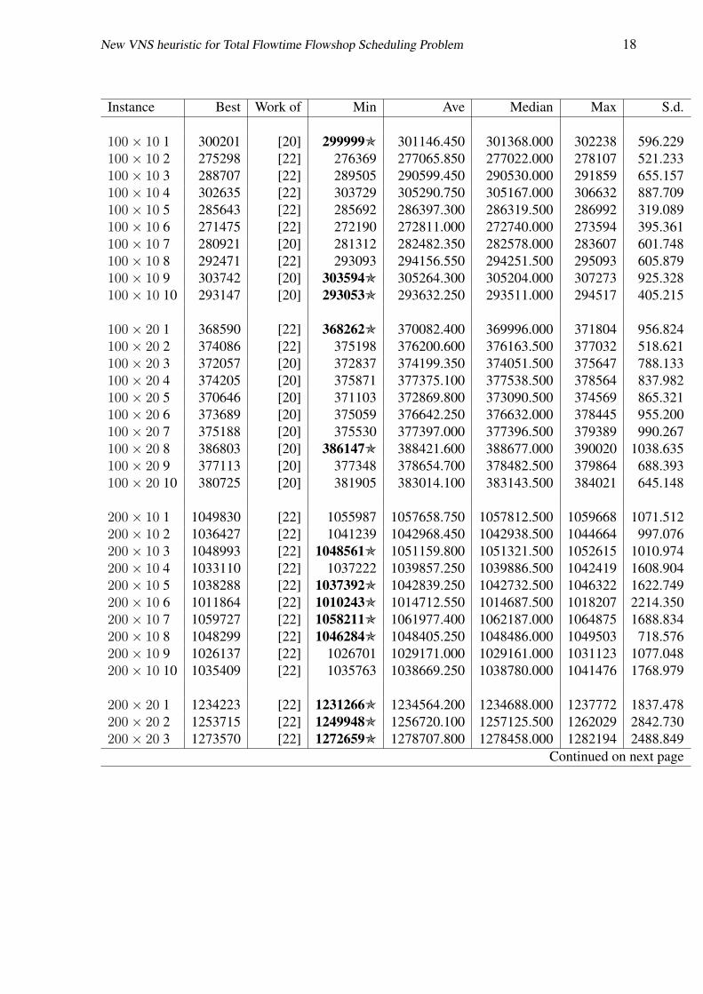
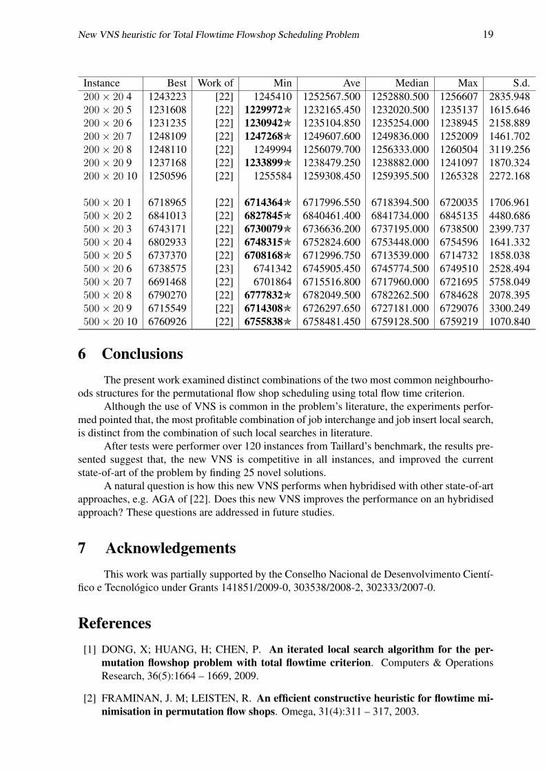
All results are summarised on table 4. The shows the name of the instance (Instance),which is denoted by n × m and an identifying integer, the best solution reported in literature(Best), the work reporting the results (Work), the minimum (Min), average (Ave), maximum(Max) and standard deviation (S.d.) achieved after 20 executions.

The VNS approach achieves the best know solution in 32 instances, plus 25 novel soluti-ons. The proposed method find all 30 best know solutions for all instances with n = 20 job. Italso ties with HGLS of [21] on instance 50× 05 number 4, and 50× 20 number 9. However themajor contribution of VNS are the novel solutions, contributing to state-of-art of the problem,indicated with a star symbol (O) next to it. There are three novel solutions for instances with100 × 10, two in the group with 100 × 20, five in group with 200 × 10, seven in group with200× 20 and eight in the group 500× 20.

Tabela 4: Results obtained after 20 executions of V NS_4 over each of 120 instances from [18].Instance Best Work of Min Ave Median Max S.d.20× 05 1 14033 [19] 14033 14037.000 14037.000 14041 4.10420× 05 2 15151 [16] 15151 15151.000 15151.000 15151 0.000

Continued on next page


Instance Best Work of Min Ave Median Max S.d.20× 05 3 13301 [19] 13301 13302.800 13301.000 13313 4.39620× 05 4 15447 [19] 15447 15447.000 15447.000 15447 0.00020× 05 5 13529 [16] 13529 13529.000 13529.000 13529 0.00020× 05 6 13123 [16] 13123 13123.000 13123.000 13123 0.00020× 05 7 13548 [19] 13548 13548.000 13548.000 13548 0.00020× 05 8 13948 [19] 13948 13948.000 13948.000 13948 0.00020× 05 9 14295 [19] 14295 14295.000 14295.000 14295 0.00020× 05 10 12943 [19] 12943 12943.000 12943.000 12943 0.000

20× 10 1 20911 [19] 20911 20911.000 20911.000 20911 0.00020× 10 2 22440 [16] 22440 22440.000 22440.000 22440 0.00020× 10 3 19833 [16] 19833 19833.000 19833.000 19833 0.00020× 10 4 18710 [19] 18710 18736.200 18747.000 18751 16.12020× 10 5 18641 [19] 18641 18641.000 18641.000 18641 0.00020× 10 6 19245 [16] 19324 19324.000 19324.000 19324 0.00020× 10 7 18363 [19] 18363 18363.000 18363.000 18363 0.00020× 10 8 10241 [16] 20241 20261.400 20241.000 20309 31.97120× 10 9 20330 [16] 20330 20330.000 20330.000 20330 0.00020× 10 10 21320 [16] 21320 21320.000 21320.000 21320 0.000

20× 20 1 33623 [16] 33623 33646.700 33623.000 33781 57.88320× 20 2 31587 [8] 31587 31587.000 31587.000 31587 0.00020× 20 3 33920 [16] 33920 33920.000 33920.000 33920 0.00020× 20 4 31661 [8] 31661 31661.000 31661.000 31661 0.00020× 20 5 34557 [8] 34557 34578.250 34557.000 34629 29.41020× 20 6 32564 [8] 32564 32564.000 32564.000 32564 0.00020× 20 7 32922 [16] 32922 32922.000 32922.000 32922 0.00020× 20 8 32412 [8] 32412 32412.000 32412.000 32412 0.00020× 20 9 33600 [8] 33600 33604.800 33600.000 33612 6.03120× 20 10 32262 [8] 32262 32263.800 32262.000 32271 3.694

50× 05 1 64803 [21] 64851 64928.900 64915.000 65083 65.75750× 05 2 68051 [20] 68083 68225.850 68232.500 68396 90.73650× 05 3 63162 [20] 63195 63402.650 63417.500 63563 100.89550× 05 4 68241 [21] 68241 68536.250 68565.000 68656 107.04150× 05 5 69360 [20] 69392 69563.400 69570.500 69691 74.02950× 05 6 66841 [20] 66865 67054.450 67053.000 67263 92.844



Instance Best Work of Min Ave Median Max S.d.50× 05 7 66253 [22] 66273 66421.300 66415.000 66635 96.48650× 05 8 64365 [20] 64381 64572.500 64579.000 64694 79.93150× 05 9 62981 [21] 63062 63151.700 63162.500 63201 39.30650× 05 10 68811 [21] 68884 69111.700 69118.000 69258 100.364

50× 10 1 87143 [20] 88100 88222.700 88225.000 88313 83.80150× 10 2 82820 [21] 83042 83259.950 83241.000 83483 119.71950× 10 3 79987 [21] 80104 80325.450 80291.500 80657 140.34950× 10 4 86466 [21] 86600 86939.300 86954.500 87181 151.82350× 10 5 86391 [21] 86655 86825.850 86829.000 87082 124.85850× 10 6 86682 [21] 86848 87025.850 87008.000 87369 112.71050× 10 7 88811 [21] 89020 89405.150 89385.500 89687 178.12350× 10 8 86839 [21] 86848 87145.950 87105.000 87503 191.77150× 10 9 85548 [21] 85555 85994.650 86004.000 86355 210.85050× 10 10 87998 [20] 88214 88559.200 88559.500 89020 226.665

50× 20 1 125831 [7] 125852 126393.400 126449.500 127008 358.37450× 20 2 119247 [7] 119270 119638.000 119597.000 120253 260.24250× 20 3 116459 [21] 116792 117171.700 117133.000 117766 267.59950× 20 4 120766 [21] 120972 121531.400 121546.000 122081 291.52150× 20 5 118405 [22] 118636 119072.600 119026.000 119575 204.61550× 20 6 120703 [20] 120792 121278.800 121240.500 121634 237.85150× 20 7 123018 [21] 123237 123781.300 123812.000 124478 345.52450× 20 8 122520 [21] 122723 123259.500 123303.000 123772 258.53150× 20 9 121872 [21] 121872 122467.450 122455.500 123170 277.67350× 20 10 124079 [20] 124182 124687.600 124699.000 125463 307.934

100× 05 1 253926 [22] 254271 254665.350 254669.500 255020 179.851100× 05 2 242886 [22] 243266 243748.100 243732.000 244155 259.702100× 05 3 238280 [22] 238452 238773.850 238743.500 239161 178.067100× 05 4 228169 [22] 228494 228873.500 228909.500 229248 216.875100× 05 5 240810 [22] 241008 241564.800 241612.500 242037 281.953100× 05 6 232876 [22] 233277 233749.600 233740.500 234203 259.043100× 05 7 240918 [20] 241165 241437.950 241409.000 241757 159.167100× 05 8 231716 [20] 231782 232255.900 232229.000 232803 252.885100× 05 9 248679 [22] 248652 249353.750 249375.000 249885 272.027100× 05 10 243518 [22] 243822 244358.200 244349.000 244985 251.794



Instance Best Work of Min Ave Median Max S.d.

100× 10 1 300201 [20] 299999O 301146.450 301368.000 302238 596.229100× 10 2 275298 [22] 276369 277065.850 277022.000 278107 521.233100× 10 3 288707 [22] 289505 290599.450 290530.000 291859 655.157100× 10 4 302635 [22] 303729 305290.750 305167.000 306632 887.709100× 10 5 285643 [22] 285692 286397.300 286319.500 286992 319.089100× 10 6 271475 [22] 272190 272811.000 272740.000 273594 395.361100× 10 7 280921 [20] 281312 282482.350 282578.000 283607 601.748100× 10 8 292471 [22] 293093 294156.550 294251.500 295093 605.879100× 10 9 303742 [20] 303594O 305264.300 305204.000 307273 925.328100× 10 10 293147 [20] 293053O 293632.250 293511.000 294517 405.215

100× 20 1 368590 [22] 368262O 370082.400 369996.000 371804 956.824100× 20 2 374086 [22] 375198 376200.600 376163.500 377032 518.621100× 20 3 372057 [20] 372837 374199.350 374051.500 375647 788.133100× 20 4 374205 [20] 375871 377375.100 377538.500 378564 837.982100× 20 5 370646 [20] 371103 372869.800 373090.500 374569 865.321100× 20 6 373689 [20] 375059 376642.250 376632.000 378445 955.200100× 20 7 375188 [20] 375530 377397.000 377396.500 379389 990.267100× 20 8 386803 [20] 386147O 388421.600 388677.000 390020 1038.635100× 20 9 377113 [20] 377348 378654.700 378482.500 379864 688.393100× 20 10 380725 [20] 381905 383014.100 383143.500 384021 645.148

200× 10 1 1049830 [22] 1055987 1057658.750 1057812.500 1059668 1071.512200× 10 2 1036427 [22] 1041239 1042968.450 1042938.500 1044664 997.076200× 10 3 1048993 [22] 1048561O 1051159.800 1051321.500 1052615 1010.974200× 10 4 1033110 [22] 1037222 1039857.250 1039886.500 1042419 1608.904200× 10 5 1038288 [22] 1037392O 1042839.250 1042732.500 1046322 1622.749200× 10 6 1011864 [22] 1010243O 1014712.550 1014687.500 1018207 2214.350200× 10 7 1059727 [22] 1058211O 1061977.400 1062187.000 1064875 1688.834200× 10 8 1048299 [22] 1046284O 1048405.250 1048486.000 1049503 718.576200× 10 9 1026137 [22] 1026701 1029171.000 1029161.000 1031123 1077.048200× 10 10 1035409 [22] 1035763 1038669.250 1038780.000 1041476 1768.979

200× 20 1 1234223 [22] 1231266O 1234564.200 1234688.000 1237772 1837.478200× 20 2 1253715 [22] 1249948O 1256720.100 1257125.500 1262029 2842.730200× 20 3 1273570 [22] 1272659O 1278707.800 1278458.000 1282194 2488.849



Instance Best Work of Min Ave Median Max S.d.200× 20 4 1243223 [22] 1245410 1252567.500 1252880.500 1256607 2835.948200× 20 5 1231608 [22] 1229972O 1232165.450 1232020.500 1235137 1615.646200× 20 6 1231235 [22] 1230942O 1235104.850 1235254.000 1238945 2158.889200× 20 7 1248109 [22] 1247268O 1249607.600 1249836.000 1252009 1461.702200× 20 8 1248110 [22] 1249994 1256079.700 1256333.000 1260504 3119.256200× 20 9 1237168 [22] 1233899O 1238479.250 1238882.000 1241097 1870.324200× 20 10 1250596 [22] 1255584 1259308.450 1259395.500 1265328 2272.168

500× 20 1 6718965 [22] 6714364O 6717996.550 6718394.500 6720035 1706.961500× 20 2 6841013 [22] 6827845O 6840461.400 6841734.000 6845135 4480.686500× 20 3 6743171 [22] 6730079O 6736636.200 6737195.000 6738500 2399.737500× 20 4 6802933 [22] 6748315O 6752824.600 6753448.000 6754596 1641.332500× 20 5 6737370 [22] 6708168O 6712996.750 6713539.000 6714732 1858.038500× 20 6 6738575 [23] 6741342 6745905.450 6745774.500 6749510 2528.494500× 20 7 6691468 [22] 6701864 6715516.800 6717960.000 6721695 5758.049500× 20 8 6790270 [22] 6777832O 6782049.500 6782262.500 6784628 2078.395500× 20 9 6715549 [22] 6714308O 6726297.650 6727181.000 6729076 3300.249500× 20 10 6760926 [22] 6755838O 6758481.450 6759128.500 6759219 1070.840

6 ConclusionsThe present work examined distinct combinations of the two most common neighbourho-

ods structures for the permutational flow shop scheduling using total flow time criterion.Although the use of VNS is common in the problem’s literature, the experiments perfor-

med pointed that, the most profitable combination of job interchange and job insert local search,is distinct from the combination of such local searches in literature.

After tests were performer over 120 instances from Taillard’s benchmark, the results pre-sented suggest that, the new VNS is competitive in all instances, and improved the currentstate-of-art of the problem by finding 25 novel solutions.

A natural question is how this new VNS performs when hybridised with other state-of-artapproaches, e.g. AGA of [22]. Does this new VNS improves the performance on an hybridisedapproach? These questions are addressed in future studies.

7 AcknowledgementsThis work was partially supported by the Conselho Nacional de Desenvolvimento Cientí-

fico e Tecnológico under Grants 141851/2009-0, 303538/2008-2, 302333/2007-0.

References[1] DONG, X; HUANG, H; CHEN, P. An iterated local search algorithm for the per-

mutation flowshop problem with total flowtime criterion. Computers & OperationsResearch, 36(5):1664 – 1669, 2009.

[2] FRAMINAN, J. M; LEISTEN, R. An efficient constructive heuristic for flowtime mi-nimisation in permutation flow shops. Omega, 31(4):311 – 317, 2003.


[3] FRAMINAN, J. M; LEISTEN, R; RUIZ-USANO, R. Efficient heuristics for flowshopsequencing with the objectives of makespan and flowtime minimisation. EuropeanJournal of Operational Research, 141(3):559–569, 2002.

[4] GRAHAM, R; LAWLER, E; LENSTRA, J; KAN, A. R. Optimization and approxi-mation in deterministic sequencing and scheduling: A survey. Annals of DiscreteMathematics, 5:287 – 326, 1979.

[5] HANSEN, P; MLADENOVIC, N. Variable neighborhood search for the p-median.Location Sci, 5:207 – 226, 1997.

[6] HANSEN, P; MLADENOVIC, N; PÉREZ, J. A. M. Variable neighbourhood search:methods and applications. Operations Research, p. 319 – 360, 2008.

[7] JARBOUI, B; EDDALY, M; SIARRY, P. An estimation of distribution algorithm forminimizing the total flowtime in permutation flowshop scheduling problems. Com-puters & Operations Research, 36(9):2638 – 2646, 2009.

[8] JARBOUI, B; IBRAHIM, S; SIARRY, P; REBAI, A. A combinatorial particle swarmoptimisation for solving permutation flowshop problems. Computers and IndustrialEngineering, 54:526 — 538, 2008.

[9] LIAO, C.-J; TSENG, C.-T; LUARN, P. A discrete version of particle swarm optimiza-tion for flowshop scheduling problems. Computers & Operations Research, 34:3099 –3111, 2007.

[10] LIU, J; REEVES, C. R. Constructive and composite heuristic solutions to the p//∑ci

scheduling problem. European Journal of Operational Research, 132:439 – 452, 2001.

[11] MURATA, T; ISHIBUCHI, H; TANAKA, H. Genetic algorithms for flowshop schedu-ling problems. Computers & Industrial Engineering, 30(4):1061 – 1071, 1996.

[12] NAGANO, M. S; MOCCELLIN, J. V. Reducing mean flow time in permutation flowshop. Journal of the Operational Research Society, 59:1700 – 1707, 2007.

[13] NAGANO, M. S; RUIZ, R; LORENA, L. A. N. A constructive genetic algorithm forpermutation flowshop scheduling. Computers & Industrial Engineering, 55(1):195 –207, 2008.

[14] RAJENDRAN, C. Heuristic algorithm for scheduling in a flowshop to minimize totalflowtime. International Journal of Production Economics, 29:65 – 73, 1993.

[15] RAJENDRAN, C; ZIEGLER, H. An efficient heuristic for scheduling in a flowshop tominimize total weighted flowtime of jobs. European Journal of Operational Research,103:129 – 138, 1997.

[16] RAJENDRAN, C; ZIEGLER, H. Ant-colony algorithms for permutation flowshopscheduling to minimize makespan/total flowtime of jobs. European Journal of Operati-onal Research, 155:426 – 438, 2004.

[17] RUIZ, R; STÜTZLE, T. A simple and effective iterated greedy algorithm for theflowshop scheduling problem. European Journal of Operational Research, 177(3):2033–2049, 2007.


[18] TAILLARD, E. D. Benchmarks for basic scheduling problems. European Journal ofOperational Research, 64:278 – 285, 1993.

[19] TASGETIREN, M. F; LIANG, Y.-C; SEVKLI, M; GENCYILMAZ, G. A particle swarmoptimization algorithm for makespan and total flowtime minimization in the per-mutation flowshop sequencing problem. European Journal of Operational Research,177:1930 – 1947, 2007.

[20] TASGETIREN, M. F; PAN, Q.-K; SUGANTHAN, P. N; CHEN, A. H.-L. A discreteartificial bee colony algorithm for the permutation flow shop scheduling problemwith total flowtime criterion. In: PROCEEDINGS OF THE IEEE WORLD CONGRESSON COMPUTATIONAL INTELLIGENCE (WCCI-2010), p. 137–144. IEEE, 2010.

[21] TSENG, L.-Y; LIN, Y.-T. A hybrid genetic local search algorithm for the permutationflowshop scheduling problem. European Journal of Operational Research, 198(1):84–92,Oct. 2009.

[22] XU, X; XU, Z; GU, X. An asynchronous genetic local search algorithm for the permu-tation flowshop scheduling problem with total flowtime minimization. Expert Systemswith Applications, In Press:–, 2010.

[23] ZHANG, Y; LI, X; WANG, Q. Hybrid genetic algorithm for permutation flowshopscheduling problems with total flowtime minimization. European Journal of Operatio-nal Research, 169(3):869 – 876, 2009.

[24] ZHANG, Y; LI, X; WANG, Q; ZHU, J. Similarity based ant-colony algorithm forpermutation flowshop scheduling problems with total flowtime minimization. In:INTERNATIONAL CONFERENCE ON COMPUTER SUPPORTED COOPERATIVEWORK IN DESIGN, p. 582–589, Los Alamitos, CA, USA, April 2009. IEEE ComputerSociety.

scheduling problem - optimization online · scheduling problem wagner emanoel costa ......

Documents