scene illuminant classiﬁcation: brighter is...

Tominaga et al. Vol. 18, No. 1 /January 2001 /J. Opt. Soc. Am. A 55

Scene illuminant classification: brighter is better

Shoji Tominaga and Satoru Ebisui

Department of Engineering Informatics, Osaka Electro-Communication University, Neyagawa,Osaka 572-8530, Japan

Brian A. Wandell

Image Systems Engineering, Stanford University, Stanford, California 94305

Received January 3, 2000; revised manuscript received July 11, 2000; accepted July 28, 2000

Knowledge of the scene illuminant spectral power distribution is useful for many imaging applications, such ascolor image reproduction and automatic algorithms for image database applications. In many applicationsaccurate spectral characterization of the illuminant is impossible because the input device acquires only threespectral samples. In such applications it is sensible to set a more limited objective of classifying the illumi-nant as belonging to one of several likely types. We describe a data set of natural images with measuredilluminants for testing illuminant classification algorithms. One simple type of algorithm is described andevaluated by using the new data set. The empirical measurements show that illuminant information is morereliable in bright regions than in dark regions. Theoretical predictions of the algorithm’s classification per-formance with respect to scene illuminant blackbody color temperature are tested and confirmed by using thenatural-image data set. © 2001 Optical Society of America

OCIS code: 330.1690.

1. INTRODUCTIONThe estimation of scene illumination from image data isimportant in several color engineering applications. Inone application, color balancing for image reproduction,data acquired under one illuminant are rendered under asecond (different) illuminant. A satisfactory color repro-duction requires transforming the captured data, prior todisplay, to account for the illumination difference. Henceknowledge about the original scene illumination is a keystep in the process. A second application is image data-base retrieval. Objects with different colors can producethe same image data when captured under different illu-minants. Hence accurately retrieving objects on the ba-sis of color requires an estimate of the scene illuminant.

Here we report two new contributions to the work onilluminant classification. First, we introduce an empiri-cal data set of natural images that can be used to test il-luminant classification algorithms.1 Second, we reviewand evaluate some simple approaches to summarizingscene illumination. We focus on one method, which wecall sensor correlation, and describe some of its strengthsand weaknesses with respect to classifying illuminants ofnatural images.

2. BACKGROUNDBecause of its significance, the theory of illuminant esti-mation has a long history in the fields of color science, im-age understanding, and image processing. A variety ofmethods for estimating the illuminant spectral power dis-tribution have been proposed, and each assumes thatthere are significant physical constraints on the set ofpossible illuminant spectra.

Several illuminant estimation algorithms have ex-

0740-3232/2001/010055-10$15.00 ©

pressed the physical constraint by assuming that the po-tential spectra fall within a low-dimensional linear model.The approach is useful in cases when the set of possiblespectral power distributions are well characterized, suchas daylight illuminants.2 Linear models representstrong a priori information about the image illuminants,and accepting this knowledge in the form of a linearmodel allows the development of simple estimationalgorithms.3–9 A shortcoming of linear models is thatthey always include illuminants that are physically non-realizable or unlikely to arise in practice. Many simplelinear estimation procedures do not exclude such solu-tions, and in the presence of significant sensor noise poorperformance can result. Brainard and Freeman9 care-fully state and analyze a Bayesian analysis of the prob-lem that substantially improves upon the original formu-lation.

Finlayson et al.10 suggest another interesting approachto the problem. (We refer to their collection of papers asFHH.) They begin with the assumption that the scene il-luminant is one of a relatively small number of likely il-luminants, such as the variety of daylight and indoor con-ditions in which images are acquired. Rather thanestimating the spectral power distribution of the illumi-nant, the algorithm chooses the most likely scene illumi-nant from a fixed set. Classification rather than estima-tion is appropriate for applications, such as photography,when the vast majority of images are very likely to be cap-tured under one of a small set of scene illuminants.

In describing their algorithms, FHH emphasize twoproperties. First, the illuminant is chosen by a simplecorrelation between a summary of the image data and aprecomputed statistic that characterizes each illuminant.In fact, the algorithm draws its name, ‘‘Color by Correla-

2001 Optical Society of America

56 J. Opt. Soc. Am. A/Vol. 18, No. 1 /January 2001 Tominaga et al.

tion,’’ from this operation. Second, the algorithm oper-ates on a chromaticity representation of the data (see Ref.11, p. 1034). Hence we refer to FHH’s method as chro-maticity correlation.

Nearly all of the descriptions of the chromaticity corre-lation method are based on simulations, and these simu-lations do not include many features of natural images orreal cameras. As part of our work on illuminant estima-tion, we decided to acquire a set of natural images andmeasure the correlated color temperature to summarizethe scene illuminant. Here we describe the data set andreport on our experimental results. These analyses haveled us to propose modifications of the algorithm that wethink are essential for classifying scene illuminants accu-rately.

3. EXPERIMENTAL METHODSA. Image CaptureThe image data used in these experiments were obtainedwith a Minolta camera (RD-175). The spectral respon-sivities of this camera were measured in separate experi-ments with a monochromator (see, e.g., Ref. 8). Likemost modern cameras, the Minolta camera includesspecial-purpose processing to transform the sensor dataprior to output. For the experiments described here, thisprocessing was disabled.

When the camera is operated in this way, the transduc-tion curve that relates input intensity to digital count islinear for the three sensor types. It is still possible, how-ever, to adjust the sensor gain into one of two differentmodes. Figure 1 shows the spectral-sensitivity functionsof the camera in these two modes. In one mode, appro-priate for imaging under tungsten illumination (say, illu-minant A), the blue-sensor gain is high. In a secondmode, appropriate for imaging under daylight (D65), theblue-sensor gain is much lower. As we describe below,operating in the high blue-sensor gain improves the per-formance of the scene illuminant classification. Henceall analyses were performed in this mode. The imagesrendered as examples below have been color balancedonly for display purposes.

At the time of image acquisition, we estimated thescene illuminant color temperature by placing a referencewhite in the scene and measuring the reflected light witha spectroradiometer. The correlated color temperatureTm can be determined from the CIE (x, y) chromaticitycoordinates of the measured spectrum by using standardmethods (Wyszecki and Stiles,12, p. 225). Specification ofa single color temperature for a complex scene is only anapproximation to the complex spatial structure of the il-luminant. Given that the goal of the classification is toprovide a single estimate of the color temperature, thisempirical approximation is a necessary starting point.Methods for improving this approximation will be takenup in Section 6.

Although they are not critical for this study, it is inter-esting to note that the Minolta camera includes threeCCD sensor arrays. One array contains a striped pat-tern of red and blue sensors, and the other two arrayscomprise green sensors that are slightly shifted in the im-age plane. This arrangement provides high spatial reso-

lution for the green data set. The red and blue sensorswere interpolated linearly and were combined with thegreen data in the analyses of this paper.

Finally, to improve the quality of the measured images,each image was acquired along with a dark frame of thesame exposure duration. The dark-frame values weremeasured and subtracted from every measured image toreduce the effects of read noise in the sensors.

B. Illuminant SetThe scene illuminants chosen for classification wereblackbody radiators at color temperatures spanning2500–8500 K in 500-K increments. Blackbody radiatorsare used frequently to approximate scene illuminants in

Fig. 1. Spectral-sensitivity functions of a camera: (a) tungstenmode, (b) daylight mode.

Fig. 2. Spectral power distributions of black body radiators.


commercial imaging. Although the blackbody radiatorsare defined by a single parameter, color temperature, thespectral power distributions of these illuminants are notwell described by a one-dimensional linear model (see Fig.2). The equation of the spectral radiant power of theblackbody radiators as a function of temperature T (inkelvins) is given by the formula12

M~l! 5 c1l25@exp~c2 /lT ! 2 1#21, (1)

where c1 5 3.7418 3 10216 Wm2, c2 5 1.4388 3 1022

m K, and l is wavelength (m). The set of blackbody ra-diators includes sources whose spectral power distribu-tions are close to CIE standard lights commonly used incolor rendering, namely, illuminant A (an incandescentlamp with 2856 K) and D65 (daylight with a correlatedcolor temperature of 6504 K).

In this paper the blackbody radiators are used not toilluminate natural scenes but to calibrate the measuringsystem and estimate the illuminant.

4. COMPUTATIONAL METHODSA. Illuminant GamutThe scene illuminant classification algorithms describedhere use a set of illuminant gamuts to define the range ofsensor responses. The illuminant gamuts capture a pri-ori knowledge about the illuminants. One precomputesthe gamuts by choosing a representative set of surfacesand predicting the camera response to these surfaces un-der each illuminant. The illuminant gamuts describedbelow were created with a database of surface spectral re-flectances made available by Vrhel et al.13 together withthe reflectances of the Macbeth Color Checker. TheVrhel database consists of 354 measured reflectance spec-tra of different materials collected from Munsell chips,paint chips, and natural products. The illuminantgamut may be made larger or smaller by selecting a dif-ferent database of surface-reflectance functions.

The illuminant gamuts are computed with the threesensors described in Fig. 1. The sensor responses arepredicted with

F RGBG 5 E

400

700

S~l!M~l!F r~l!

g~l!

b~l!Gdl, (2)

where S(l) is the surface spectral-reflectance function;r(l), g(l), and b(l) are the spectral-sensitivity func-tions; and M(l) is the blackbody radiator. These(R, G, B) values are used to define the illuminant gam-uts with methods that are more fully described below.

Creation of the illuminant gamuts is a central part ofthe classification algorithms, and the engineer has someability to structure the gamuts by choosing a coordinateframe and selecting the objects that will be used to repre-sent typical surfaces. In general, the gamuts should sat-isfy two conflicting criteria. First, it is important thatthe illuminant gamuts provide good coverage of the mea-surement space. Second, when two illuminants requiredifferent image processing, it is desirable that the corre-sponding illuminant gamuts have little overlap. Smalloverlap between a pair of illuminant gamuts is an indica-tor that the algorithm should be able to discriminate well

between the illuminant pair. In considering the illumi-nant classification algorithms, we have examined severalcoordinate systems with these criteria in mind.

Finlayson11 used chromaticity coordinates to representthe gamuts: (R/B, G/B, 1) 5 (r, g, 1). Like all chro-

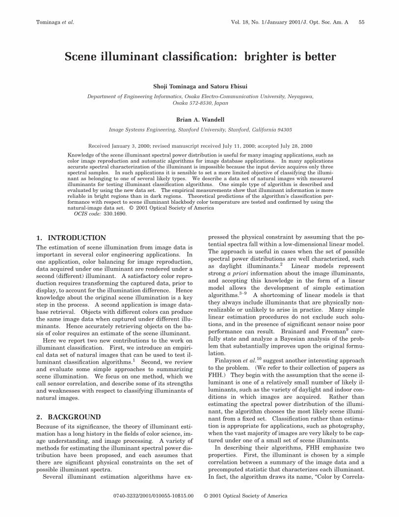
Fig. 3. Illuminant gamuts for blackbody radiators in the (r, b)chromaticity plane.

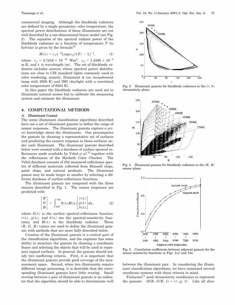
Fig. 4. Illuminant gamuts for blackbody radiators in the (R, B)sensor plane.

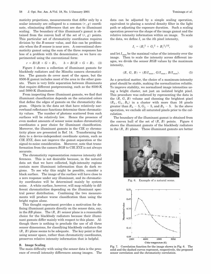
Fig. 5. Correlation coefficients between adjacent gamuts for thesensor sensitivity functions in Figs. 1(a) and 1(b).


maticity projections, measurements that differ only by ascalar intensity are collapsed to a common (r, g) coordi-nate, eliminating differences that are due to illuminantscaling. The boundary of this illuminant’s gamut is ob-tained from the convex hull of the set of (r, g) points.This particular set of chromaticity coordinates requiresdivision by the B-sensor value, and this can be problem-atic when the B sensor is near zero. A conventional chro-maticity gamut using the sum of the three responses hasless of a problem with the denominator, so we have ex-perimented using the conventional form:

r 5 R/~R 1 G 1 B !, b 5 B/~R 1 G 1 B !. (3)

Figure 3 shows a collection of illuminant gamuts forblackbody radiators and the Minolta camera chromatici-ties. The gamuts do cover most of the space, but the8500-K gamut includes most of the area in the other gam-uts. There is very little separation between illuminantsthat require different postprocessing, such as the 8500-Kand 5000-K illuminants.

From inspecting these illuminant gamuts, we find thatilluminant classification depends on the saturated colorsthat define the edges of gamuts on the chromaticity dia-gram. Objects in the data set that have relatively nar-rowband reflectance functions determine these chromatic-ity values. The number of photons scattered from suchsurfaces will be relatively low. Hence the presence ofeven modest amounts of sensor noise makes chromaticitycoordinates a poor choice for illuminant classification.Moreover, the illuminant gamuts in the CIE xy chroma-ticity plane are presented in Ref. 14. Transforming thedata to a device-independent coordinate system, such asCIE XYZ, does not improve the gamut separation or thesignal-to-noise consideration. Moreover, note that trans-formation from the camera RGB to CIE XYZ is not alwaysaccurate.

The chromaticity representation removes intensity dif-ferences. This is not desirable because, in the naturaldata set that we have collected, high-intensity regionscontain more illuminant information than do dark re-gions. To see why this might be possible, consider ablack surface. The image of the surface will have close toa zero response under any illuminant, and its chromatic-ity coordinates will be determined mainly by systemnoise. A white surface, however, will map reliably to dif-ferent chromaticities depending on the illuminant spec-tral power distribution. Combining the two measure-ments will produce worse classification than using thebright region alone.

This thought experiment provides a motivation for de-fining illuminant gamuts directly on the sensor data, say,in the RB plane. The (R, B) sensor plane is a reasonablechoice for the blackbody radiators because their illumi-nant gamuts differ mainly with respect to this plane. Al-though there is nothing to preclude the use of all threesensor dimensions, for classifying blackbody radiators the(R, B) plane seems to be adequate. The key point is thatusing sensor space, rather than chromaticity coordinates,preserves relative intensity information that is helpful.

B. Image ScalingThe main difficulty with using the sensor data is the pres-ence of overall intensity differences among images. The

data can be adjusted by a simple scaling operation,equivalent to placing a neutral density filter in the lightpath or adjusting the exposure duration. Such a scalingoperation preserves the shape of the image gamut and therelative intensity information within an image. To scalethe data, we define Ii as the ith pixel intensity,

Ii 5 ~Ri2 1 Gi

2 1 Bi2!1/2, (4)

and let Imax be the maximal value of the intensity over theimage. Then to scale the intensity across different im-ages, we divide the sensor RGB values by the maximumintensity,

~R, G, B ! 5 ~R/Imax , G/Imax , B/Imax!. (5)

As a practical matter, the choice of a maximum-intensitypixel should be stable, making the normalization reliable.To improve stability, we normalized image intensities us-ing a bright cluster, not just an isolated bright pixel.This procedure was enforced by representing the data inthe (R, G, B) volume and choosing the brightest pixel(Rb , Gb , Bb) in a cluster with more than 16 pixelsgreater than Rb 2 5, Gb 2 5, and Bb 2 5. In the aboveoperation, we exclude all saturated pixels prior to the cal-culation.

The boundary of the illuminant gamut is obtained fromthe convex hull of the set of (R, B) points. Figure 4shows the illuminant gamuts of the blackbody radiatorsin the (R, B) plane. These illuminant gamuts are better

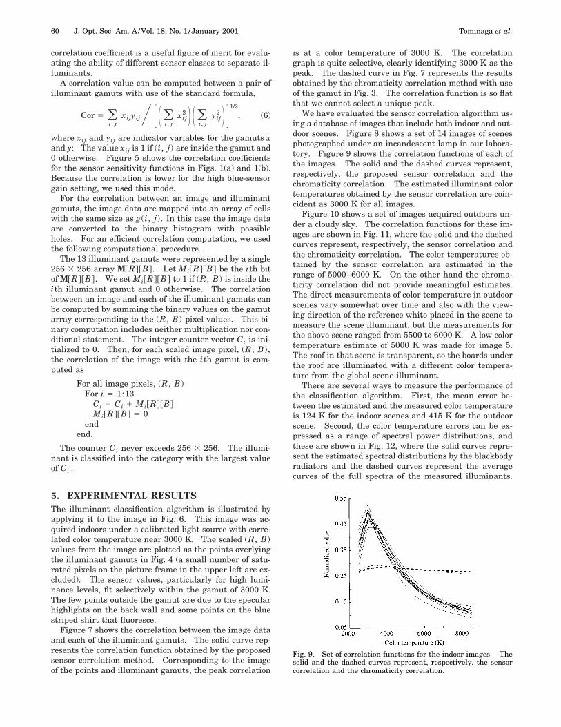
Fig. 6. Example of a natural scene.

Fig. 7. Correlation function for the image shown in Fig. 6. Thesolid and the dashed curves represent, respectively, the proposedsensor correlation and the chromaticity correlation.


Fig. 8. Set of 14 images of indoor scenes under an incandescent lamp.

separated than those in the chromaticity plane, and thebest separation occurs for high-intensity values. As wewill confirm experimentally, the dark regions contributeno significant information to the classification choice anddo not limit performance in this plane. The gamut in thesensor space comes to a point at the high end, so that nomatter what surfaces are in the image, the most intenseregions track the illuminant variation better.

C. Image and Gamut CorrelationTo quantify the overlap, either between image data andilluminant gamuts or between a pair of gamuts, we calcu-late the correlation suggested by FHH. The RB plane isdivided into a regular grid (i, j) with small even intervals(usually 256 3 256). The illuminant gamuts are repre-sented by setting a g(i, j) value to 1 or 0 depending onwhether the cell falls inside the convex hull. The gamut


correlation coefficient is a useful figure of merit for evalu-ating the ability of different sensor classes to separate il-luminants.

A correlation value can be computed between a pair ofilluminant gamuts with use of the standard formula,

Cor 5 (i, j

xijyijY FS (i, j

xij2 D S (

i, jyij

2 D G1/2

, (6)

where xij and yij are indicator variables for the gamuts xand y: The value xij is 1 if (i, j) are inside the gamut and0 otherwise. Figure 5 shows the correlation coefficientsfor the sensor sensitivity functions in Figs. 1(a) and 1(b).Because the correlation is lower for the high blue-sensorgain setting, we used this mode.

For the correlation between an image and illuminantgamuts, the image data are mapped into an array of cellswith the same size as g(i, j). In this case the image dataare converted to the binary histogram with possibleholes. For an efficient correlation computation, we usedthe following computational procedure.

The 13 illuminant gamuts were represented by a single256 3 256 array M@R#@B#. Let Mi@R#@B# be the ith bitof M@R#@B#. We set Mi@R#@B# to 1 if (R, B) is inside theith illuminant gamut and 0 otherwise. The correlationbetween an image and each of the illuminant gamuts canbe computed by summing the binary values on the gamutarray corresponding to the (R, B) pixel values. This bi-nary computation includes neither multiplication nor con-ditional statement. The integer counter vector Ci is ini-tialized to 0. Then, for each scaled image pixel, (R, B),the correlation of the image with the ith gamut is com-puted as

For all image pixels, (R, B)For i 5 1:13

Ci 5 Ci 1 Mi@R#@B#Mi@R#@B# 5 0

endend.

The counter Ci never exceeds 256 3 256. The illumi-nant is classified into the category with the largest valueof Ci .

5. EXPERIMENTAL RESULTSThe illuminant classification algorithm is illustrated byapplying it to the image in Fig. 6. This image was ac-quired indoors under a calibrated light source with corre-lated color temperature near 3000 K. The scaled (R, B)values from the image are plotted as the points overlyingthe illuminant gamuts in Fig. 4 (a small number of satu-rated pixels on the picture frame in the upper left are ex-cluded). The sensor values, particularly for high lumi-nance levels, fit selectively within the gamut of 3000 K.The few points outside the gamut are due to the specularhighlights on the back wall and some points on the bluestriped shirt that fluoresce.

Figure 7 shows the correlation between the image dataand each of the illuminant gamuts. The solid curve rep-resents the correlation function obtained by the proposedsensor correlation method. Corresponding to the imageof the points and illuminant gamuts, the peak correlation

is at a color temperature of 3000 K. The correlationgraph is quite selective, clearly identifying 3000 K as thepeak. The dashed curve in Fig. 7 represents the resultsobtained by the chromaticity correlation method with useof the gamut in Fig. 3. The correlation function is so flatthat we cannot select a unique peak.

We have evaluated the sensor correlation algorithm us-ing a database of images that include both indoor and out-door scenes. Figure 8 shows a set of 14 images of scenesphotographed under an incandescent lamp in our labora-tory. Figure 9 shows the correlation functions of each ofthe images. The solid and the dashed curves represent,respectively, the proposed sensor correlation and thechromaticity correlation. The estimated illuminant colortemperatures obtained by the sensor correlation are coin-cident as 3000 K for all images.

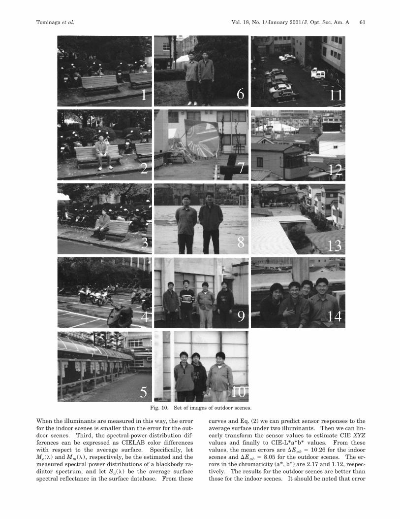
Figure 10 shows a set of images acquired outdoors un-der a cloudy sky. The correlation functions for these im-ages are shown in Fig. 11, where the solid and the dashedcurves represent, respectively, the sensor correlation andthe chromaticity correlation. The color temperatures ob-tained by the sensor correlation are estimated in therange of 5000–6000 K. On the other hand the chroma-ticity correlation did not provide meaningful estimates.The direct measurements of color temperature in outdoorscenes vary somewhat over time and also with the view-ing direction of the reference white placed in the scene tomeasure the scene illuminant, but the measurements forthe above scene ranged from 5500 to 6000 K. A low colortemperature estimate of 5000 K was made for image 5.The roof in that scene is transparent, so the boards underthe roof are illuminated with a different color tempera-ture from the global scene illuminant.

There are several ways to measure the performance ofthe classification algorithm. First, the mean error be-tween the estimated and the measured color temperatureis 124 K for the indoor scenes and 415 K for the outdoorscene. Second, the color temperature errors can be ex-pressed as a range of spectral power distributions, andthese are shown in Fig. 12, where the solid curves repre-sent the estimated spectral distributions by the blackbodyradiators and the dashed curves represent the averagecurves of the full spectra of the measured illuminants.

Fig. 9. Set of correlation functions for the indoor images. Thesolid and the dashed curves represent, respectively, the sensorcorrelation and the chromaticity correlation.


Fig. 10. Set of images of outdoor scenes.

When the illuminants are measured in this way, the errorfor the indoor scenes is smaller than the error for the out-door scenes. Third, the spectral-power-distribution dif-ferences can be expressed as CIELAB color differenceswith respect to the average surface. Specifically, letMe(l) and Mm(l), respectively, be the estimated and themeasured spectral power distributions of a blackbody ra-diator spectrum, and let Sa(l) be the average surfacespectral reflectance in the surface database. From these

curves and Eq. (2) we can predict sensor responses to theaverage surface under two illuminants. Then we can lin-early transform the sensor values to estimate CIE XYZvalues and finally to CIE-L*a* b* values. From thesevalues, the mean errors are DEab 5 10.26 for the indoorscenes and DEab 5 8.05 for the outdoor scenes. The er-rors in the chromaticity (a* , b* ) are 2.17 and 1.12, respec-tively. The results for the outdoor scenes are better thanthose for the indoor scenes. It should be noted that error


in the color temperature scale does not always correspondto color difference in the perceptually uniform scale.

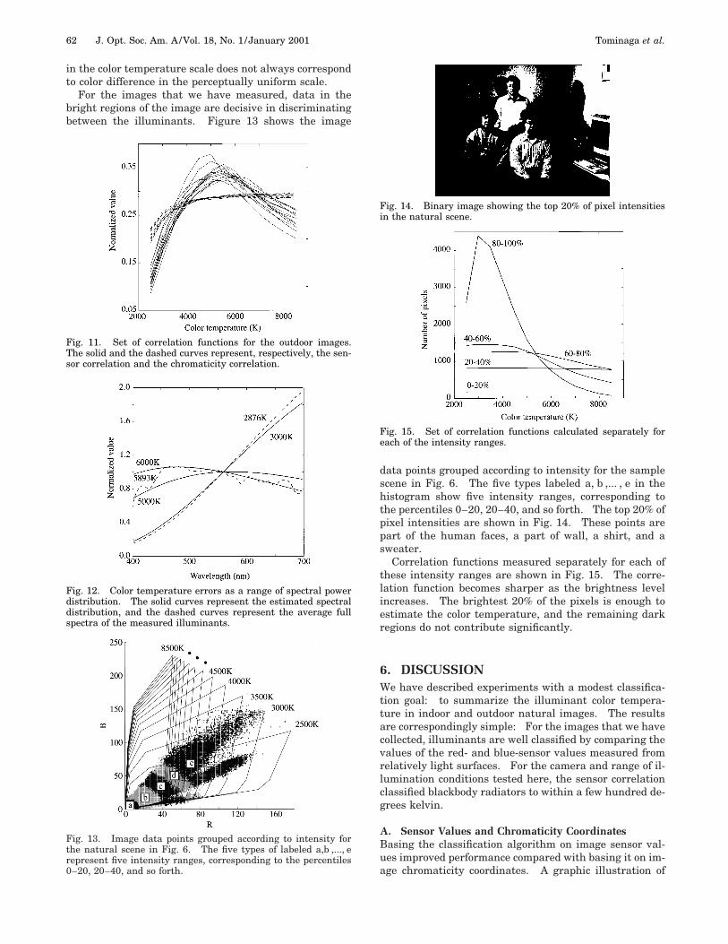
For the images that we have measured, data in thebright regions of the image are decisive in discriminatingbetween the illuminants. Figure 13 shows the image

Fig. 11. Set of correlation functions for the outdoor images.The solid and the dashed curves represent, respectively, the sen-sor correlation and the chromaticity correlation.

Fig. 12. Color temperature errors as a range of spectral powerdistribution. The solid curves represent the estimated spectraldistribution, and the dashed curves represent the average fullspectra of the measured illuminants.

Fig. 13. Image data points grouped according to intensity forthe natural scene in Fig. 6. The five types of labeled a,b ,..., erepresent five intensity ranges, corresponding to the percentiles0–20, 20–40, and so forth.

data points grouped according to intensity for the samplescene in Fig. 6. The five types labeled a, b ,... , e in thehistogram show five intensity ranges, corresponding tothe percentiles 0–20, 20–40, and so forth. The top 20% ofpixel intensities are shown in Fig. 14. These points arepart of the human faces, a part of wall, a shirt, and asweater.

Correlation functions measured separately for each ofthese intensity ranges are shown in Fig. 15. The corre-lation function becomes sharper as the brightness levelincreases. The brightest 20% of the pixels is enough toestimate the color temperature, and the remaining darkregions do not contribute significantly.

6. DISCUSSIONWe have described experiments with a modest classifica-tion goal: to summarize the illuminant color tempera-ture in indoor and outdoor natural images. The resultsare correspondingly simple: For the images that we havecollected, illuminants are well classified by comparing thevalues of the red- and blue-sensor values measured fromrelatively light surfaces. For the camera and range of il-lumination conditions tested here, the sensor correlationclassified blackbody radiators to within a few hundred de-grees kelvin.

A. Sensor Values and Chromaticity CoordinatesBasing the classification algorithm on image sensor val-ues improved performance compared with basing it on im-age chromaticity coordinates. A graphic illustration of

Fig. 14. Binary image showing the top 20% of pixel intensitiesin the natural scene.

Fig. 15. Set of correlation functions calculated separately foreach of the intensity ranges.


why this might be possible is shown in Fig. 16. This im-age illustrates the difference between sensor values andchromaticity coordinates using a simple two-dimensionalgraphical example. Panel (a) shows three image pointsin the (R, B) sensor plane. These points are plotted aschromaticity coordinates, so the original sensor measure-ments could have been made at any of the values indi-cated by the dashed lines. Panel (b) shows two possibledistributions of the original data. The left graph shows adistribution in which the chromaticity coordinates ofpoints with relatively large blue-sensor responses aremore intense. This pattern of responses would be ex-pected under a blue-sky illumination. The right graphshows a distribution in which the chromaticity coordi-nates of points with relatively large red-sensor values aremore intense. This pattern of responses would be ex-pected under a tungsten illumination. It is straightfor-ward to distinguish the intensity information, shown bythe position of the points in the left and right graphs ofpanel (b), under high and low color temperatures. Whenthe analysis begins with chromaticity coordinates, thisrelative intensity information is unavailable.

B. Surface Shape and Illuminant DistributionForsyth first introduced the canonical sensor spacegamut.15 The analysis developed in that paper includedthe assumption that surfaces are flat and that the illumi-nant does not vary over space. This might cause someconcern in applying the algorithm to natural images, yetwe have observed that neither assumption is essential tothe classification method. Surface-reflectance scaling bygeometric changes and illuminant intensity scaling byshading variation leave the convex hull of the sensorgamut unchanged. Both of these effects (illuminationscaling and variations in surface orientation) are presentin the test images, and neither effect challenges the algo-rithm.

C. LimitationsThe experiments and methods that we have describedhave several limitations. Overcoming certain of these

Fig. 16. Graphical example illustrating the difference betweensensor values and chromaticity coordinates.

limitations will require additional work, but a solutioncan be foreseen. For example, we have performed ourcalculations using only two of the three color channels.This limitation could be lifted at the cost of increasedcomputation. Also, the selection of surfaces for definingthe gamut should be refined and based on better informa-tion regarding typical pictorial content. It is also pos-sible to introduce Bayesian methods into the computa-tional procedure. The cost of using a more complexalgorithm, and the difficulty in identifying the probabili-ties of observing illuminants and surfaces within an im-age, must be weighed against the benefits of includingsuch processing.

The most serious limitation, however, concerns the im-plicit model of the scene. Although the use of a singlecolor temperature to characterize the scene illuminant isa reasonable starting point and is common practice inphotography, the approximation is not accurate. Indirectillumination scattered from large objects in the scene,shadows, transparencies, and geometrical relationshipsbetween small light sources and surface orientation allmake the image scene spatially complex. Identifying thecomplex pattern of the global illumination is needed forapplications in computer-graphics rendering (see Ref. 16).But this complexity is well beyond the illumination esti-mates derived from the simple methods described hereand serves only to raise additional research questions.

Finally, the classification method described here, likemany others in common use, is vulnerable to variabilityin the collection of scene surfaces. For any illuminant itis possible to choose a collection of surfaces that will causethe algorithm to make incorrect classifications. This vul-nerability is true of nearly all classification algorithmsthat have been proposed to date. Human perception ap-pears to be less susceptible to this type of error (see, e.g.,Ref. 17), and the size and potential significance of the gapbetween algorithm and human performance will be inter-esting to explore.

ACKNOWLEDGMENTSThis work was supported by Dainippon Screen MFG, Ja-pan, and support was provided to the Stanford Program-mable Digital Camera program by Agilent, Canon, East-man Kodak, Hewlett-Packard, Intel, and IntervalResearch corporations. We thank Y. Nayatani, H. Hel-Or, M. Bax, J. DiCarlo, and J. Farrell for useful discus-sions and comments on the manuscript.

Address correspondence to Shoji Tominaga, Depart-ment of Engineering Informatics, Osaka Electro-Communication University, Neyagawa, Osaka 572-8530,Japan. E-mail, [email protected]; phone, 81-72-820-4562; fax, 81-72-824-0014.

REFERENCES1. The image data used in this paper will be available at

http://www.osakac.ac.jp/labs/shoji/.2. D. B. Judd, D. L. MacAdam, and W. S. Stiles, ‘‘Spectral dis-

tribution of typical daylight as a function of correlated colortemperature,’’ J. Opt. Soc. Am. 54, 1031–1040 (1964).

3. L. T. Maloney and B. A. Wandell, ‘‘Color constancy: amethod for recovering surface spectral reflectance,’’ J. Opt.Soc. Am. A 3, 29–33 (1986).


4. S. Tominaga and B. A. Wandell, ‘‘The standard surface re-flectance model and illuminant estimation,’’ J. Opt. Soc.Am. A 6, 576–584 (1989).

5. B. V. Funt, M. S. Drew, and J. Ho, ‘‘Color constancy frommutual reflection,’’ Int. J. Comput. Vis. 6, 5–24 (1991).

6. M. D’Zmura and G. Iverson, ‘‘Color constancy: I. Basictheory of two-stage linear recovery of spectral descriptionsfor lights and surfaces,’’ J. Opt. Soc. Am. A 10, 2148–2165(1993).

7. M. D’Zmura, G. Iverson, and B. Singer, ‘‘Probabilistic colorconstancy,’’ in R. D. Luce et al., eds., Geometric Representa-tions of Perceptual Phenomena (Erlbaum, Mahway, N.J.,1995), pp. 187–202.

8. S. Tominaga, ‘‘Multichannel vision system for estimatingsurface and illumination functions,’’ J. Opt. Soc. Am. A 13,2163–2173 (1996).

9. D. H. Brainard and W. T. Freeman, ‘‘Bayesian color con-stancy,’’ J. Opt. Soc. Am. A 14, 1393–1411 (1997).

10. G. D. Finlayson, P. M. Hubel, and S. Hordley, ‘‘Color by cor-relation,’’ in Proceedings of the Fifth Color Imaging Confer-ence (Society for Imaging Science and Technology, Spring-field, Va., 1997), pp. 6–11.

11. G. D. Finlayson, ‘‘Color in perspective,’’ IEEE Trans. Pat-tern Anal. Mach. Intell. 18, 1034–1038 (1996).

12. G. Wyszecki and W. S. Stiles, Color Science: Concepts andMethods, Quantitative Data and Formulae (Wiley, NewYork, 1982).

13. M. J. Vrhel, R. Gershon, and L. S. Iwan, ‘‘Measurement andanalysis of object reflectance spectra,’’ Color Res. Appl. 19,4–9 (1994).

14. S. Tominaga, S. Ebisui, and B. A. Wandell, ‘‘Color tempera-ture estimation of scene illumination,’’ in Proceedings of theSeventh Color Imaging Conference (Society for Imaging Sci-ence and Technology, Springfield, Va., 1999), pp. 42–47.

15. D. A. Forstyth, ‘‘A novel algorithm for color constancy,’’ Int.J. Comput. Vis. 5, 5–36 (1990).

16. Y. Yu, P. Debevec, J. Malik, and T. Hawkins, ‘‘Inverse glo-bal illumination: recovering reflectance models of realscenes from photographs,’’ Special Interest Group on Com-puter Graphics and Interactive Techniques (SIGGRAPH)99, 215–224 (1999).

17. D. H. Brainard, ‘‘Color constancy in the nearly natural im-age. 2. Achromatic loci,’’ J. Opt. Soc. Am. A 15, 307–325(1998).

scene illuminant classiﬁcation: brighter is...

Documents