scenario based water resources model to support policy making · scenario based water resources...
TRANSCRIPT

Scenario Based Water Resources
Model to Support Policy Making

Scenario Based Water Resources Model to Support Policy Making
November 2008
Client World Bank
Authors Peter Droogers
Chris Perry
Report FutureWater: 79
FutureWater
Costerweg 1G
6702 AA Wageningen
The Netherlands
+31 (0)317 460050
www.futurewater.nl

Contents
1 Introduction 3
2 Models 5 2.1 Concepts 5
2.1.1 Introduction 5 2.1.2 Concepts of modelling 7 2.1.3 Model classification 8 2.1.4 Existing model overviews 9 2.1.5 Model reviews 10
2.2 WEAP model 11 2.2.1 Background 11 2.2.2 WEAP approach 12 2.2.3 Program structure 13
3 Scen Basin 17
4 Scen Basin Results 21 4.1 Base Line 21 4.2 Scenario: Climate Change 24 4.3 Intervention: Advanced Irrigation Technique 24 4.4 Intervention: Improve Domestic Use 25 4.5 Intervention: Land Use Changes 25 4.6 Intervention: sustainable groundwater use 25 4.7 Comparison of scenarios 26
5 Conclusions and Recommendations 31
6 References 33
Appendix 1: Tutorial Output Analysis 35 Introduction 35 Basin-wide water balance 37 Irrigated areas 43
Appendix 2: WEAP Tips and Tricks 46
2

1 Introduction Appropriate planning in water resources, and more specifically in irrigation, is becoming increasingly important given the challenges of already-stressed water resources, climate change, growing population, increase in prosperity, potential food shortages, etc. However, policy makers and planners are often constrained, in this context of increasing complexity, by insufficient knowledge and tools to evaluate the consequences of alternative interventions and thus make the appropriate decisions. Furthermore, important misconceptions often underlie strategies proposed to address these problems. To illuminate these issues, a scenario-based policy oriented demonstration model is presented here. The term “model” here refers more to a demonstration tool rather than a software package. The model as developed includes physical processes, but at a lumped and parametric level. Most importantly, the model will focus on scenario1 and intervention analysis, so that policy makers can better understand and evaluate the impact and interactions of a certain change or decision they plan to make, and the changing environment in which they are operating. The objective of this study is to: Present a scenario-based water resources model that enables policy makers to explore the impact of interventions and changes at the basin level. The report starts with a general overview of the use of simulation models in water resources planning. Since this report focuses on scenario analysis, the WEAP model will be explained in more detail. Chapter 3 will introduce a hypothetical basin to be used to demonstrate the use of scenario analysis models. The actual scenario analysis is presented in Chapter 4. The report ends with conclusions and recommendations for the future. Finally, Appendix 1 describes a hands-on tutorial to practice concepts described in this manual.
1 The terms scenario and intervention are loosely used. Similar terms used as well are: coping strategy, story line, impact analysis. It is important to distinguish between an external change (eg climate) that cannot be controlled by the relevant decision maker, and an intervention that can be controlled. Obviously, this is decision maker specific. E.g. a water manager would see climate change as an external change, while world leaders would see this as a process they can influence (at least in principle).
3

4
2 Models
2.1 Concepts
2.1.1 Introduction
Water related problems are diverse and location specific, but water shortage is frequently the most pressing issue. Increasing international and intersectoral competition for scarce water, in the context of growing demand for food, and uncertain impacts of climate change is a central challenge for the next decades. Seckler et al. (1999) estimated that by 2025 cereal production will have to increase by 38% to meet world food demands. The World Water Vision, an outcome from the Second World Water Forum in The Hague in 2000, estimated a similar figure of 40% based on various projections and modelling exercises (Cosgrove and Rijsberman, 2000). These figures were more or less confirmed by projections based on an econometric model which showed that the rate of increase of grain demand will be about 2% per year for the 2000-2020 period (Koyama, 1998). To produce this increasing amount of food, substantial amounts of water are required. Global estimates of water consumption by sector indicate that irrigated agriculture consumes 85% from all the withdrawals and that this consumptive use will increase by 20% in 2025 (Shiklomanov, 1998). Gleick (2000) presented estimates on the amount of water required to produce daily food diets per region. According to his figures large differences can be found between regions ranging from 1,760 liters per day per person for Sub-Saharan Africa to 5,020 for North America. Differences come from the larger number of calories consumed and the higher fraction of water-intensive meat in the diet of a North American. This increase in food and water requirements coincides with a growing evidence of existing water scarcity. A study by the United Nations (UN, 1997) revealed that one-third of the world’s total population of 5.7 billion lives under conditions of relative water scarcity and 450 million people are under severe water stress. Relative Water Demand (RWD) is expressed as the fraction water demand over water supply. A RWD greater then 0.2 is classified as relative water scarce, while a RWD greater then 0.4 as severe water stress. However, these values as mentioned by the UN are based on national-level totals, ignoring the fact that huge spatial differences occur, especially within larger countries. Vörösmarty et al. (2000) showed that including these in-country differences, 1.8 billion people live in areas with sever water stress. Using their global water model and some projections for climate change, population growth and economic growth, they concluded that the number of people living in sever water stress will have grown to 2.2 billion by the year 2025. A study published by the International Water Management Institute (Seckler et al., 1999), based on country analysis, indicated that by the year 2025, 8 percent of the population of countries studied (India and China where treated separately, because of their extreme variations within the country) will have major water scarcity problems. Countries accounting for 80% of the study population need to increase withdrawals to meet future requirements, and only for 12% of the population is no action required. Although the exact numbers on how severe water stress actually is, or will be in the near future, and how much more food we should produce, differ to some extent, the main trend is unambiguous: more water for food and water will be scarcer.
5

These references address the global scale, but at smaller scales--countries, regions and basins--policymakers face difficult choices in addressing their water problems. This, in combination with the “think globally, act locally” principle, makes the basin the most appropriate scale to focus on. Data are essential to assess the current condition of water resources and to understand past trends. However, to explore options for the future tools are required that are able to explore the impact of future trends and how we can adapt to these in the most sustainable way. Simulation models are the appropriate tools to do these analyses. R.K Linsley, a pioneer in the development of hydrologic simulation at Stanford University wrote already in 1976: “In summary then it can be said that the answer to ‘Why simulate?’ is given by the following points:
1. Simulation is generally more adequate because it involves fewer approximations than conventional [ie physically-based] methods.
2. Simulation gives a more useful answer because it gives a more complete answer. 3. Simulation allows adjustment for change that conventional methods cannot do
effectively. 4. Simulation costs no more than the use of reliable conventional methods (excluding
empirical formulae which should not be used in any case). 5. Data for simulation is easily obtained on magnetic tape from the Climatic Data Service
or the Geological Survey. 6. No more work or time is required to complete a simulation study than for a thorough
hydrologic analysis with conventional methods. Often the time and cost requirements are less.
7. In any case, if the time and cost are measured against the quality and completeness of the results, simulation is far ahead of the conventional techniques.
8. Even though the available data are limited, simulation can still be useful because the data are used in a physically rational computational program.”
These points are still valid today, and can be more or less summarised by the two main objectives of model application: (i) understanding processes and how they interact, and (ii) scenarios analyses. Understanding processes is something that starts at during model development. In order to build our models we must have a clear picture on how processes in the real world function and how we can mimic these in our models. The main challenge is not in trying to build in all processes we understand, which is in fact impossible, but lies in our capability to simplify things and concentrate on the most relevant processes of the model under construction. The main reason for the success of models in understanding processes is that models can provide output over an unlimited time-scale, at an unlimited spatial resolution, and for difficult to observe sub-processes (e.g. Droogers and Bastiaanssen, 2002). These three items are the weak point in experiments, but are at the same time exactly the components in the concept of sustainable water resources management. The most important aspect of applying models, however, is in their use to explore different scenarios. These scenarios can capture aspects that cannot directly be influenced, such as population growth and climate change (Droogers and Aerts, 2005). These are often referred to as projections. Contrary to this are the management scenarios or interventions where water
6
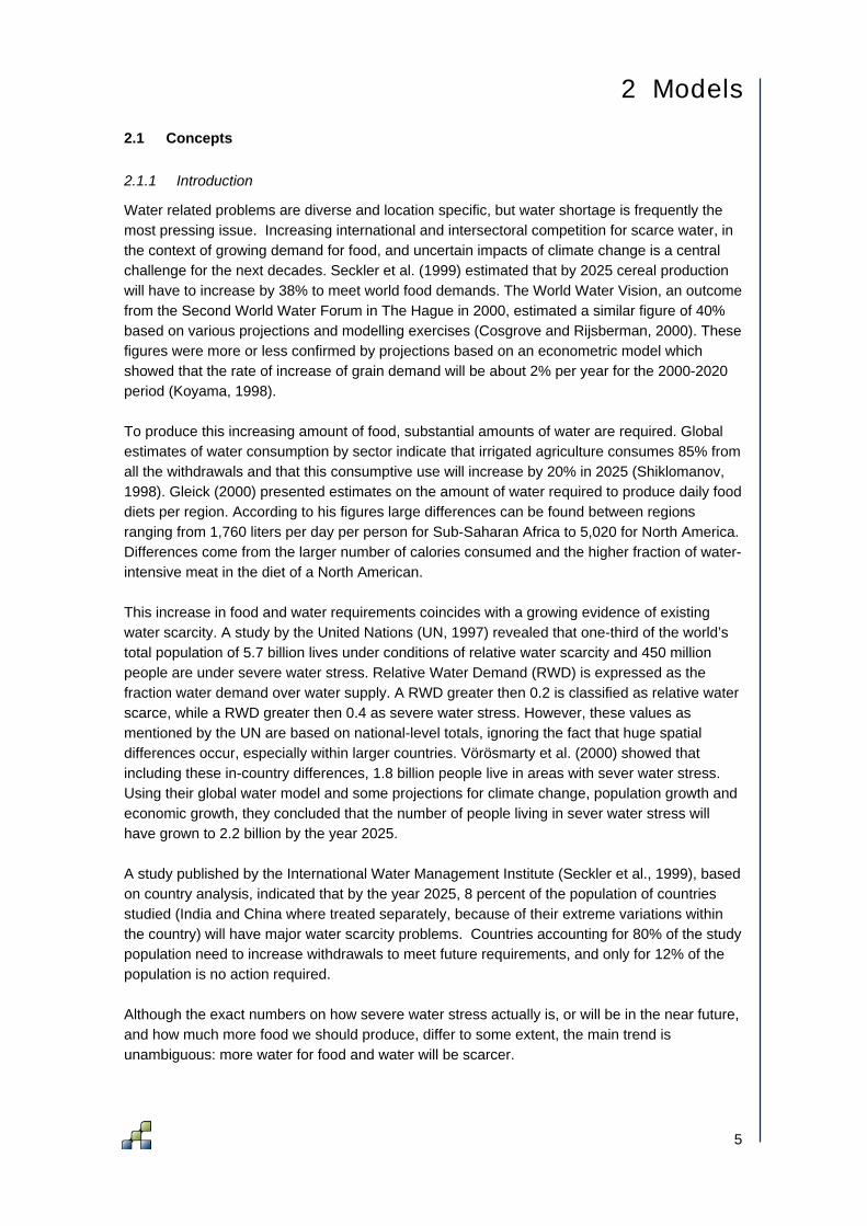
managers and policy makers can make decisions that will have a direct impact. Examples are changes in reservoir operation rules, water allocation between sectors, investment in infrastructure such as water treatment or desalinization plants, and agricultural/irrigation practices. In other words: models enable to change focus from a re-active towards a pro-active approach. (Figure 1).
Understand current water resources
Understand past water resources
Options for future- technical- socio-economic- policy oriented
Trend
•Remote Sensing•Observations•Analysis•Statistics
•Models?
Past
Today
Future
Figure 1. The concept of using simulation models in scenario analysis.
2.1.2 Concepts of modelling
The term modelling is broad and includes everything where reality is imitated. The Webster dictionary distinguishes 13 different meanings for the word “model”: where the following definition is most close to the one this study is focusing on: “a system of postulates, data, and inferences presented as a mathematical description of an entity or state of affairs”. However, we will restrict our definition here to computer models and that a model should have a certain degree of process-oriented approach, excluding statistical, regression oriented models. This leads to the following definition: “a model is a computer based mathematical representation of dynamic processes”. The history of hydrological and agro-hydrological models, based on this somewhat restricted definition, is relatively short. One of the first models is the so-called Stanford Watershed Model (SWM) developed by Crawford and Linsley in 1966, but the main principles are still used in current catchment models to convert rainfall into runoff. SWM did not have much physics included as the catchment was just represented by a set of storage reservoirs linked to each other. The value of parameters describing the interaction between these different reservoirs was obtained by trying to optimise the simulated and the observed streamflows. At the other end of the spectrum are the field-scale models describing unsaturated flow processes in the soil and root water uptake. One of the first to be developed was the SWATR model by Feddes et al. (1978) based on Richards’ equation. Since these models are based on points and use the concept that unsaturated flow is dominated only by vertical transport of water, much more physics could be built in from the beginning. A huge number of hydrological models exist, and applications are growing rapidly. The number of pages on the Internet including “hydrological model” is over 1.2 million (using Google on January 2007). Using the same search engine with “water resources model” provides 86 million pages found (Figure 2). A critical question for hydrological model studies is therefore related to the selection of the most appropriate model. One of the most important issues to consider is the spatial scale to be incorporated in the study and how much physical detail to be included. Figure 3 illustrates the negative correlation between the physical detail of the model applied and spatial
7

scale of application. The figure indicates also the position of commonly used models in this continuum.
Figure 2. Number of pages returned with “water resources model” (January 2007).
Figure 3. Spatial and physical detail of hydrological models.
2.1.3 Model classification
The number of existing hydrological simulation models is probably in the tens of thousands. Even if we exclude the one-off models developed for a specific study and count only the more generic applied models it must exceed a thousand. Some existing model overviews include numerous models: IRRISOFT (2000): 105, USBR (2002): 100, CAMASE (2005): 211, and REM (2006): 675, amongst others. Interesting is that there seems to be no standard model or models emerging in catchment modelling, contrary to for example in groundwater modelling where ModFlow is the de-facto standard. Two hypotheses for this lack of standard can be brought forward. The first one is that model development is still in its initial phase, despite some 25 years of history, and therefore it is easy to start developing one’s own model that can compete with similar existing ones with a reasonable amount of time and effort--indeed a serious scientist is considered to have his/her own model or has at least developed one during his or her PhD studies. A second possible reason for the large number of models might be that hydrological
8

processes are so complex and diverse that each case requires its specific model or set of models. It is therefore interesting to see how models can be classified and see whether such a classification might be helpful in selecting the appropriate model given a certain question or problem to be solved. Probably, the most generally used classification is the spatial scale the model deals with and the amount of physics included (Figure 3). These two characteristics determine such other model characteristics as data need, expected accuracy, required expertise, and user-friendliness amongst others.
2.1.4 Existing model overviews
A substantial number of overviews exist listing available models and providing a short summary of each. Most of this information is provided by the developers of the model themselves and tends therefore to be biased towards the capabilities of the model. The most commonly referenced overviews are discussed briefly here, keeping in mind that these are changing rapidly, in size and number, since the Internet provides almost unlimited options to start and update such an overview in a automatic or semi-automatic way. A clear example is the Hydrologic Modelling Inventory project from the United States Bureau of Reclamation, where about 100 mainly river basin models are registered by model developers (USBR, 2002). An overview of agro-ecosystem models is provided by a consortium named CAMASE (Concerted Action for the development and testing of quantitative Methods for research on Agricultural Systems and the Environment; CAMASE, 2005). The following types of models are distinguished: crop science, soil science, crop protection, forestry, farming systems, and land use studies, environmental science, and agricultural economics. A total of 211 models are included and for each model a nice general overview is provided. Unfortunately the last update of the register was in 1996 and advances in model development over the last decade are not taken into account. The United States Geological Survey (USGS, 2006) provides an overview of all their own models (about 50) divided into five categories: geochemical, groundwater, surface water, water quality, and general. Some of the models are somewhat outdated, but some commonly used ones are included too. All the models are in the public domain and can be used without restrictions. For most of the models source code is provided as well. The United States Department of Agriculture also provides models to be used in crop-water related issues. The National Water and Climate Center of the USDA has an irrigation page (NWCC, 2006) with some water management tools related to field scale irrigation. The United States Environmental Protection Agency is very active in supporting model development. The SWAT model, originating from their research programs, might have the potential to become the de-facto standard in basin scale modelling, and has been included in the BASINS package (BASINS, 2006). More linkages to models and other model overviews are provided too (EPA, 2006). Modelling efforts of USGS, USDA, USACE, and EPA, combined with some other models, are brought together by the USGS Surface water quality and flow Modelling Interest Group (SMIG,
9

2006a). SMIG has set up the most complete references to model archives nowadays including links to 40 archives (SMIG, 2006b). The most up-to-date overview of models using crop growth modelling is the Register of Ecological Models (REM, 2006), with 675 models as of 12-Dec-2005. Besides this overview of models the same website provides general conceptual definitions and links to other websites about modelling.
2.1.5 Model reviews
In the previous section an overview of existing model inventories has been given. Although useful as a catalogue it does not provide any independent guide to model quality. The “best” model does not exist: selection is a function of the application and questions to be answered. A few studies have been undertaken where a limited number of models have been thoroughly tested and reviewed. The majority of these studies focus on two or three models that are rather similar in nature and in most cases it was concluded that the models perform comparably. A survey of Australian catchment managers, model users and model developers revealed the following conclusions about the state of catchment modelling in the late 1990's (http://www.catchment.crc.org. au/toolkit/current.htm):
• There are almost as many models as there are modellers, and there is significant duplication of effort in model building.
• The standard of computer code employed in these models, and their supporting documentation is generally poor.
• User interfaces are generally poor and inconsistent in their design and function. • There are no agreed standards on how to code, document and deliver the models to
end-users. • Virtually no holistic modelling is being undertaken at large spatial scales, partly due to
the lack of a suitable paradigm for linking models. • Access to many catchment models is restricted.
This negative viewpoint is to a certain extent still valid, although a some modelling tools have overcome most of these shortcomings. However, the perspective of many water managers is still quite suspicious about model application and only by demonstration projects can those views change. The Texas Natural Resource Conservation Commission evaluated 19 river basin models, referred to as Water Availability Models, in order to select the most suitable model for management of water resources, including issuing new water right permits (TNRCC, 1998). A total of 26 evaluation criteria were identified as important functions and characteristics for selecting a model that fits the needs of the 23 river basins in Texas. Most important was the ability of the model to support water rights simulation. During the evaluation process, each model was assessed and ranked in order of its ability to meet each criterion. The 19 models in the first phase narrowed down to five: WRAP, MODSIM, STATEMOD, MIKE BASIN, and OASIS. Models not selected included WEAP (no appropriation doctrine) and SWAT (not intuitive and user-friendly). The final conclusion was to use the WRAP model with the HEC-PREPRO GUI. As mentioned, the study focused only on models able to assist in water rights questions.
10

A similar study was performed to select an appropriate river basin model to be used by the Mekong River Commission (MRC, 2000). In fact, it was already decided that considering the requirements of the MRC not one single model could fulfil the needs, but three different types of model were necessary: hydrological (rainfall-runoff), basin water resources, and hydrodynamic. Three main criteria were used to select the most appropriate model: technical capability, user friendliness, and sustainability. Considering the hydrological models 11 were evaluated and the SWAT model was considered as the most suitable one. Since water quality and sediment processes were required models like SLURP were not selected. Interesting is that grid based models were not recommended as they were considered as relatively new. The selected basin simulation model was IQQM. ISIS was reviewed as the best model to be used to simulate the hydrodynamic processes. An actual model comparison, where models were really tested using existing data, was initiated by the Hydrology Laboratory (HL) of the National Weather Service (NWS), USA. The comparison is limited to hydrological models and their ability to reproduce hydrographs, based on detailed radar rainfall data. This model comparison, referred to as DMIP (Distributed Model Intercomparison Project, 2002) has the intention to invite the academic community and other researchers to help guide the NWS's distributed modelling research by participating in a comparison of distributed models applied to test data sets. Results have been published recently, but no clear conclusions were drawn (Reed et al., 2004). For the purpose of this study the WEAP model is recommended as the most appropriate tool. WEAP follows an integrated approach to water development that places water supply projects in the context of multi-sectoral, prioritised demands, and water quality and ecosystem preservation and protection. WEAP incorporates these values into a practical tool for water resources planning and policy analysis. WEAP places demand-side issues such as water use patterns, equipment performance, re-use strategies, costs, and water allocation schemes on an equal footing with supply-side topics such as stream flow, groundwater resources, reservoirs, and water transfers. WEAP is also distinguished by its integrated approach to simulating both the natural (e.g. rainfall, evapo-transpirative demands, runoff, baseflow) and engineered components (e.g. reservoirs, groundwater pumping) of water systems, allowing the planner access to a more comprehensive view of the broad range of factors that must be considered in managing water resources for present and future use. WEAP is an effective tool for examining alternative water development and management options.
2.2 WEAP model
2.2.1 Background
WEAP is short for Water Evaluation and Planning System. It is a microcomputer tool for integrated water resources planning. It provides a comprehensive, flexible and user-friendly framework for policy analysis (SEI, 2005). Many regions face formidable freshwater management challenges. Allocation of limited water resources, environmental quality, and policies for sustainable water use are issues of increasing concern. Conventional supply-oriented simulation models are not always adequate. Over the last decade, an integrated approach to water development has emerged that places water
11

supply projects in the context of demand-side issues, water quality and ecosystem preservation. WEAP aims to incorporate these values into a practical tool for water resources planning.
WEAP is distinguished by its integrated approach to simulating water systems and by its policy orientation. WEAP is a desktop laboratory for examining alternative water development and management strategies (SEI, 2005).
2.2.2 WEAP approach
WEAP is operating on the basic principles of a water balance. The analyst represents the system in terms of its various supply sources (e.g. rainfall, rivers, creeks, groundwater, and reservoirs); withdrawal, transmission and wastewater treatment facilities; ecosystem requirements, water demands and pollution generation. The data structure and level of detail can easily be customised to meet the requirements of a particular analysis, and to reflect the limits imposed by available data. Operating on these basic principles WEAP is applicable to many scales; municipal and agricultural systems, single catchments or complex transboundary river systems. WEAP not only incorporates water allocation but also water quality and ecosystem preservation modules. This makes the model suitable for simulating many of the fresh water problems that exist in the world nowadays (SEI, 2005a).
WEAP applications generally involve several steps. The study definition sets up the time frame, spatial boundary, system components and configuration of the problem. The Current Accounts, which can be viewed as a calibration step in the development of an application, provide a snapshot of the actual water demand, pollution loads, resources and supplies for the system. Key assumptions may be built into the Current Accounts to represent policies, costs and factors that affect demand, pollution, supply and hydrology. Scenarios build on the Current Accounts and allow exploration of the impact of alternative assumptions or policies on future water availability and use. Finally, the Scenarios are evaluated with regard to water sufficiency, costs and benefits, compatibility with environmental targets, and sensitivity to uncertainty in key variables (SEI, 2005). WEAP calculates a water and pollution mass balance for every node and link in the system. Water is dispatched to meet instream and consumptive requirements, subject to demand priorities, supply preferences, mass balance and other constraints. Point loads of pollution into receiving bodies of water are computed, and instream concentrations of polluting elements are calculated. WEAP operates on a monthly time step, from the first month of the Current Accounts year through the last month of the last Scenario year. Each month is independent of the previous month, except for reservoir and aquifer storage. Thus, all of the water entering the system in a month (e.g. head flow, groundwater recharge, or runoff into reaches) is either stored in an aquifer or reservoir, or leaves the system by the end of the month (e.g. outflow from end of river, demand site consumption, reservoir or river reach evaporation, transmission and return flow link losses). Because the time scale is relatively long (monthly), all flows are assumed to occur instantaneously. Thus, a demand site can withdraw water from the river, consume some, return the rest to a wastewater treatment plant that treats it and returns it to the river. This return flow is available for use in the same month to downstream demands (SEI, 2005b).
12

Each month the calculations (algorithms) follow this order (SEI, 2005b):
1. Annual demand and monthly supply requirements for each demand site and flow requirement.
2. Runoff and infiltration from catchments, irrigation. 3. Inflows and outflows of water for every node and link in the system. This includes
calculating withdrawals from supply sources to meet demand, and dispatching reservoirs. This step is solved by a linear program (LP), which attempts to optimise coverage of demand site and instream flow requirements, subject to demand priorities, supply preferences, mass balance and other constraints.
4. Pollution generation by demand sites, flows and treatment of pollutants, and loadings on receiving bodies, concentrations in rivers.
5. Hydropower generation. 6. Capital and operating costs and revenues.
2.2.3 Program structure
WEAP consists of five main views: (i) schematic, (ii) data, (iii) results, (iv) overviews, and (v) notes. These views are listed as graphical icons on the “View Bar”, located on the left of the screen. Click an icon in the View Bar to select one of the views. For the Results and Overviews view, WEAP will calculate scenarios before the view is displayed, if any changes have been made to the system or the scenarios.
Figure 4. Example of the WEAP Schematic view.
2.2.3.1 Schematic view
In the Schematic view the basic structure of the model is created (Figure 4). Objects from the item menu are dragged and dropped into the system. First the river is created and the demand sites and supply sites are positioned appropriately in the system. Pictorial files can be added as
13
a background layer. The river, demand sites and supply sites are linked to each other by transmission links, runoff/infiltration links or return flow links.
2.2.3.2 Data view
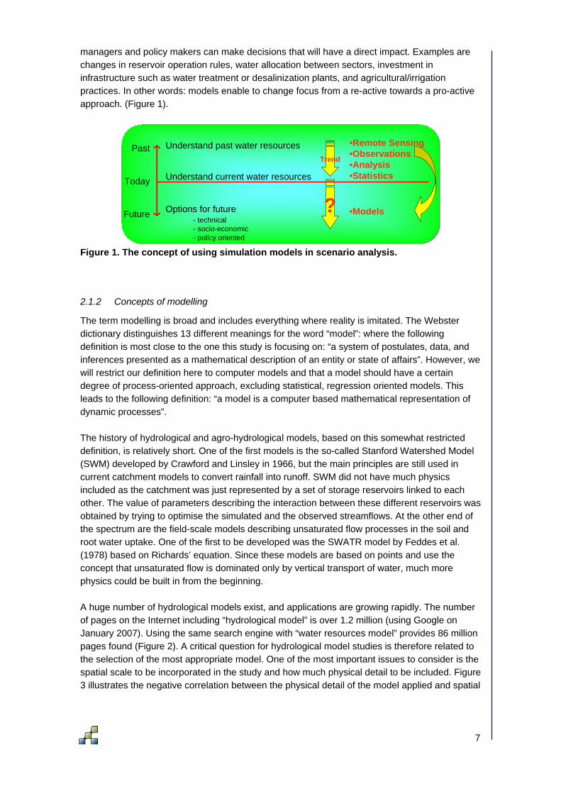
Adding data to the model is done in the Data view. The Data view is structured as a data tree with branches. The main branches are named Key assumptions, Demand sites, Hydrology, Supply and Resources and Water quality. The objects created in the Schematic view are shown in the branches. Further subdivisions of a demand site can be created by the analyst. The example in Figure 5 shows further sub-division of the demand sites into land use classes. The Data view allows creation of variables and relationships, entering assumptions and projections using mathematical expressions, and dynamically linking to input files (SEI, 2005).
Figure 5. Example of the WEAP Data view.
2.2.3.3 Result view
Clicking the Results view will force WEAP to run its monthly simulation and report projections of all aspects of the system, including demand site requirements and coverage, streamflow, instream flow requirement satisfaction, reservoir and groundwater storage, hydropower generation, evaporation, transmission losses, wastewater treatment, pollution loads, and costs. The Results view is a general purpose reporting tool for reviewing the results of scenario calculations in either chart or table form, or displayed schematically (Figure 6). Monthly or yearly results can be displayed for any time period within the study horizon. The reports are available either as graphs, tables or maps and can be saved as text, graphic or spreadsheet files. Each report can be customised by changing: the list of nodes displayed (e.g. demand sites), scenarios, time period, graph type, unit, gridlines, color, or background image. Customised reports can be saved as a "favorite" for later retrieval. Up to 25 "favorites" can be displayed side
14

by side by grouping them into an "overview". Using favorites and overviews, the user can easily assemble a customised set of reports that highlight the key results of the analysis (Figure 7). In addition to its role as WEAP's main reporting tool, the Results view is also important as the main place where intermediate results can be analysed to ensure that data, assumptions and models are valid and consistent. The reports are grouped into five main categories:
• Demand • Supply and Resources • Catchments • Water Quality • Financial
Details about output generated by WEAP can be found in Table 1. This Table indicates also the processes that are included in WEAP and to which level of detail output can be obtained.
Figure 6. Example of the WEAP Results view.
Figure 7. Example of the WEAP Overviews view.
15
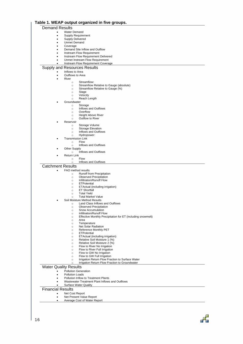
Table 1. WEAP output organized in five groups. Demand Results
• Water Demand • Supply Requirement • Supply Delivered • Unmet Demand • Coverage • Demand Site Inflow and Outflow • Instream Flow Requirement • Instream Flow Requirement Delivered • Unmet Instream Flow Requirement • Instream Flow Requirement Coverage
Supply and Resources Results • Inflows to Area • Outflows to Area • River
o Streamfiow: o Streamfiow Relative to Gauge (absolute) o Streamfiow Relative to Gauge (%) o Stage o Velocity o Reach Length
• Groundwater o Storage o Inflows and Outflows o Overflow o Height Above River o Outflow to River
• Reservoir o Storage Volume o Storage Elevation o Inflows and Outflows o Hydropower:
• Transmission Link o Flow o Inflows and Outflows
• Other Supply o Inflows and Outflows
• Return Link o Flow o Inflows and Outflows
Catchment Results • FAO method results
o Runoff from Precipitation o Observed Precipitation o Infiltration/Runoff Flow o ETPotential o ETActual (including irrigation) o ET Shortfall o Total Yield o Total Market Value
• Soil Moisture Method Results o Land Class Inflows and Outflows o Observed Precipitation o Snow Accumulation o Infiltration/Runoff Flow o Effective Monthly Precipitation for ET (including snowmelt) o Area o Temperature o Net Solar Radiation o Reference Monthly PET o ETPotential o ETActual (including irrigation) o Relative Soil Moisture 1 (%) o Relative Soil Moisture 2 (%) o Flow to River No Irrigation o Flow to River Full Irrigation o Flow to GW No Irrigation o Flow to GW Full Irrigation o Irrigation Return Flow Fraction to Surface Water o Irrigation Return Flow Fraction to Groundwater
Water Quality Results • Pollution Generation • Pollution Loads • Pollution Inflow to Treatment Plants • Wastewater Treatment Plant Inflows and Outflows • Surface Water Quality
Financial Results • Net Cost Report • Net Present Value Report • Average Cost of Water Report
16

3 Scen Basin The model developed for this study is, given the scope of the project, based on a hypothetical river basin. The choice of a hypothetical basin, rather than a real one, was made to ensure that the focus will be on conceptual issues, and not on the capabilities of the model to mimic reality—which has been demonstrated in other applications of the model. For this exercise, this is an essential consideration, given that the vast majority of papers published in water resources journals end with the final conclusion “the model was able to simulate the observed stream flows”. Here, we are demonstrating the capacity to capture impacts and explore alternatives—and it is generally agreed that the relative accuracy of a model (= comparing base line to scenarios) is higher than the absolute accuracy (= comparing observed to simulated flows). This point is hardly explored in literature, but essential for policy making support (Droogers et al., 2008). To ensure that the hypothetical basin has a degree of realism, it is based on a real river basin in Northern-Africa. To keep the focus of the model on conceptual issues, simplifications and generalizations have been made. The hypothetical basin will be referred to as Scen Basin. Main characteristics of Scen Basin are:
• Area 3,600,000 ha • Population: 7 millions • Four catchment areas • Irrigated area: 300,000 ha • Annual rainfall: 600 mm (Figure 10) • Annual ETref: 1500 mm (Figure 10)
Catch03
Catch02
Catch01
Catch04
60 km60 km
Figure 8. Scen Basin including the four catchment areas.
17

Figure 9. Scen Basin as represented in WEAP. To represent Scen Basin in WEAP the following schematic notes were created (Figure 9):
• 1 main river and 3 tributaries • 3 towns • 2 main irrigation schemes
o Irri01 = 50,000 ha o Irri02 = 250,000 ha
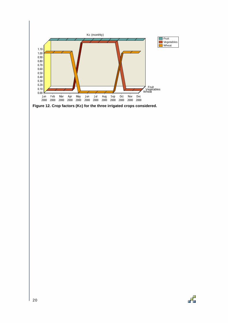
• 4 catchment areas • 3 irrigated crops
o winter wheat o summer vegetables o fruits
• 2 reservoirs o Res01: 3700 MCM o Res01: 6000 MCM
• 1 aquifer Some input for the model can be seen in the following Figures.
18

Precipitation (monthly)
Jan2000
Feb2000
Mar2000
Apr2000
May2000
Jun2000
Jul2000
Aug2000
Sep2000
Oct2000
Nov2000
Dec2000
mm
/mon
th
100
90
80
70
60
50
40
30
20
10
0
ETref (monthly)
Jan2000
Feb2000
Mar2000
Apr2000
May2000
Jun2000
Jul2000
Aug2000
Sep2000
Oct2000
Nov2000
Dec2000
mm
180
160
140
120
100
80
60
40
20
0
Figure 10. Monthly precipitation and ETref.
Figure 11. Typical example of input screen in WEAP: area for catchments and irrigation systems.
19
FruitVegetablesWheat
Kc (monthly)
Jan2000
Feb2000
Mar2000
Apr2000
May2000
Jun2000
Jul2000
Aug2000
Sep2000
Oct2000
Nov2000
Dec2000
1.101.000.900.800.700.600.500.400.300.200.100.00
FruitVegetables
Wheat
Figure 12. Crop factors (Kc) for the three irrigated crops considered.
20

4 Scen Basin Results
4.1 Base Line
The model as described in the previous chapter is applied to obtain results for the so-called base line: the current situation. Results of the base line will than be compared to a set of scenarios (external changes) and interventions (changes influenced by decision makers). A comparison between the base line, scenarios and interventions must be based on relevant indicators. The model has been set up to run for five successive years, all assuming similar conditions. These five years were run to ensure that the model reaches an equilibrium stage and results are not affected by initial conditions. Only results of the last year (2005) were considered. The following set of indicators has been defined to compare the different scenario results:
• Basin wide o Total precipitation (MCM/y) o Basin outflow (MCM/y) o Reservoir changes (MCM/y) o Aquifer changes (MCM/y) o Total consumption (MCM/y) o Water demand (MCM/y)
• Irrigation o ETpotential (MCM/y) o Actual crop transpiration (MCM/y) o Actual soil evaporation (MCM/y) o ETshortfall (MCM/y)
• Domestic o Demand (MCM/y) o Unmet demand (MCM/y)
The actual value of these indicators can be obtained from the Results tab of the WEAP interface (see for a detailed tutorial Appendix 1):
• Basin wide o Total precipitation
Catchments > Observed Precipitation
o Basin outflow Supply and Resources > Rivers > River > Streamflow > 24 \ Reach
o Reservoir changes (= Dec 2005 - Dec 2004) Supply and Resources > Reservoirs > Storage Volumes (select only Res01 and Res02)
o Aquifer changes (= Dec 2005 - Dec 2004) Supply and Resources > Groundwater > Storage
o Total Consumption Demand > Demand Sites Inflows and Outflows > Consumption
o Total demand Demand > Water Demand
• Irrigated agriculture
21

o ET actual Catchments > ETActual (select: Levels 2 and Group)
o ET shortage Catchments > ET Shortfall
Key output of the model will be presented here by some Figures. Actual numbers belonging to these indicators can be found in Table 2. The main results and conclusions for the base line (current) situation indicate:
• In the model the catchment areas with the forests and the shrublands are considered as water demanders as well. It is not only the irrigation and domestic/industry demanding water.
• Irrigation is not the major consumer of water, but forests and natural vegetation are. Consumption of urban water is very low.
• There is an overall water shortage in the basin while at the same time there is outflow to the sea. There are some unavoidable losses (fast runoff from rainfall, sewerage, timing) and there might be some losses that might be reduced.
• Aquifer levels are declining quite rapidly. • From the irrigated areas water is consumed beneficial by crop transpiration, but quite
some water is lost unbeneficial by soil evaporation.
Catch01 Catch02 Catch03 Catch04 City01 City02 City03 Irri01 Irri02
Water Demand (not including loss, reuse and DSM)Scenario: Actual, All months
2005
Bill
ion
Cub
ic M
eter
11.0
10.0
9.0
8.0
7.0
6.0
5.0
4.0
3.0
2.0
1.0
0.0
Figure 13. Results Base Line: annual demand for each area.
22

Forest Fruit Rainfed Shrubland Vegetables Wheat
ETActual (including irrigation)Scenario: Actual, All months
2005
Milli
on C
ubic
Met
er
9,000
8,5008,0007,500
7,0006,5006,000
5,5005,000
4,5004,0003,500
3,0002,5002,000
1,5001,000
5000
Figure 14. Results Base Line: annual actual evapotranspiration per vegetation type.
Irri01 Irri02
Demand Site Coverage (% of requirement met)Scenario: Actual, All months
Jan2005
Feb2005
Mar2005
Apr2005
May2005
Jun2005
Jul2005
Aug2005
Sep2005
Oct2005
Nov2005
Dec2005
Per
cent
100
90
80
70
60
50
40
30
20
10
0
Figure 15. Results Base Line: water supply as percentage of water requirements.
23

24. Reach
Streamflow (below node or reach listed)Scenario: Actual, All months, River: Scen
Jan2005
Feb2005
Mar2005
Apr2005
May2005
Jun2005
Jul2005
Aug2005
Sep2005
Oct2005
Nov2005
Dec2005
Mill
ion
Cub
ic M
eter
180
160
140
120
100
80
60
40
20
0
Figure 16. Results Base Line: outflow to the sea.
4.2 Scenario: Climate Change
It is expected that climate change will have a substantial impact on water resources. The IPCC (Intergovernmental Panel on Climate Change) in its latest fourth Assessment Report published climate change projections. For the country where the Scen Basin is located the projections for the end of this century indicate that precipitation will decrease by 30 to 50%. At the same time temperatures are expected to increase by about 3 to 4 degrees, which will increase water requirements and potential evapotranspiration substantially. This has been implemented in WEAP by the following assumptions:
• Precipitation: decrease by 40% WEAP > Data > Key Assumptions > Climate > Rainfall > 600 360 mm
• Potential evapotranspiration: increase by 20% WEAP > Data > Key Assumptions > Climate > ETref > 1500 1800 mm
4.3 Intervention: Advanced Irrigation Technique
Modernization of irrigation systems is often considered as a viable intervention to overcome water shortages. Moreover, modernization opens the way to expand even the existing areal of irrigated agriculture. WEAP is not developed to study detailed irrigation technologies, but is using a lumped approach to irrigation systems. However, WEAP is very strong in exploring interactions with all other water resources and water demands within a basin. Improved irrigation techniques are in WEAP represented by two processes: non-beneficial soil evaporation and percolation to groundwater. By introducing advanced irrigation systems, like
24

pressurized systems, we assume that non-beneficial soil evaporation can be reduced by 50% (from 20% to 10%), and fraction of irrigation water available to the plant increased from 50% to 80%. This is implemented in WEAP as:
• Soil evaporation WEAP > Data > Key Assumptions > IrrigationSystems > Elosses > 20% 10%
• Irrigations WEAP > Data > Key Assumptions > IrrigationSystems > IrrigationFraction >
50% 20%
These assumed water savings are accompanied by an extension of the irrigation area. Since losses are reduced by 20%, one would expect that an increase in the irrigated area by 20% will be logical. This is implemented in WEAP as:
• Expanded areal irrigation WEAP > Data > Demand Sites and Catchments > Irr01 > 50,000 ha 50,000 *
1.2 ha WEAP > Data > Demand Sites and Catchments > Irr02 > 250,000 ha 250,000
* 1.2 ha
Appendix 2 provides more information on how these advanced irrigation techniques are actually implemented and processed by WEAP.
4.4 Intervention: Improve Domestic Use
In the base line model 100 liter water per person per day is provided for drinking water. A very extreme intervention is assumed where this 100 liter is reduced by 50% to 50 liter per person per day:
• Reduce domestic supply WEAP > Data > Key Assumptions > City > Allocation > 36.5 18.25 m3
4.5 Intervention: Land Use Changes
To improve the quality of the catchments extensive reforestation is planned. In the current situation 50% of the catchment is covered by forests and 40% by shrubland. It is explored what the impact would be on water resources if half of the shrublands will be converted to forests.
• Increase forest area WEAP > Data > Demand Sites and Catchments > Catch0x > forest > 50% 70% WEAP > Data > Demand Sites and Catchments > Catch0x > shrub > 40% 20%
4.6 Intervention: sustainable groundwater use
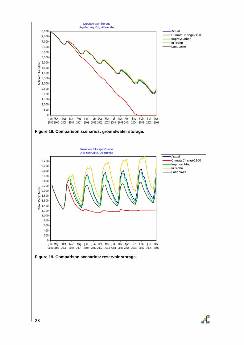
Table 2 and Figure 18 demonstrate that groundwater depletion is a real problem in the basin. On an annual base overexploitation is in the order of 900 MCM for all scenarios. Therefore drastic interventions have to be taken to ensure sustainable groundwater use.
25
Firstly, it is important to understand the groundwater dynamics. In Figure 20 total inflows and outflows of the groundwater is depicted. The irrigation systems is the major extractor of the groundwater, extractions from the city are very low. In terms of recharge the natural catchment plays a key role and percolation from the upstream irrigation system contributes by about 100 MCM per year. Depletion of the groundwater is in fact one of the major sources for the downstream irrigation system. The intervention of introducing advanced irrigation systems reduces the percolation of the upstream irrigation system resulting in even less water available for the groundwater. Only drastic measures such as reducing abstraction can make groundwater extraction sustainable. In Figure 21 groundwater levels for the current situation and three levels of conservation abstraction show that groundwater extraction has to be reduced substantially to make the system sustainable.
4.7 Comparison of scenarios
Summary results of the comparison between the scenarios are shown by some Figures hereafter and summarized in Table 2. It should be emphasized again that results are obtained from a hypothetical basin and also input for the scenarios was conducted using global knowledge rather than site specific information. However, it has been proven that for scenario analysis the concept of relative accuracy (comparing scenarios) in contrast to actual accuracy (comparing observations with simulation), assure that results as presented reflects a good indication of trends (Bormann, 2005; Droogers et al., 2008). Results as presented can be summarized by:
• Climate change will have a tremendous impact on the basin. Aquifer levels will drop down, overall water shortage will increase and irrigated agricultural production will decrease substantial. One should keep in mind that for this specific basin climate change will alter rainfall substantially (minus 30%).
• The irrigation technology intervention will have a positive impact on the overall basin water resources. The assumed saving of water by 40% (10% by reducing soil evaporation and 30% by drainage and seepage reduction) is in reality much lower. Main reason is that quite some of these interventions reduce reuse of water, rather than leading to real water savings. In fact only the reduction in soil evaporation and the reduced outflow to the sea might be considered as real savings.
• The assumed reduction in urban water consumption by 50% has hardly any impact on the basin as a whole.
• Finally the forestation of some of the shrublands have quite some impact on the water resources in the basin. Forests transpire more water than shrublands resulting in overall increasing water shortage. Obviously, these forest might provide eco-services that are not included in the current model. The potential positive impact on soil erosion of forestation is also not considered.
26

Table 2. Indicator values for all scenarios Basin wide Base Line CC2100 IrrTech Urban Landcover
Total precipitation (MCM/y) 21,600 12,960 21,960 21,600 21,600 Basin outflow (MCM/y) 2,659 1,161 2,034 2,635 2,399 Reservoir changes (MCM/y) 0 -10 0 0 0 Aquifer changes (MCM/y) -931 0 -861 -920 -951 Total consumption (MCM/y) 18,011 11,789 19,066 18,046 18,249 Unmet demand (MCM/y) 38,614 59,912 36,656 38,546 41,118
Irrigation ETpotential (MCM/y) 5,917 6,470 6,476 5,924 5,786 Tactual (MCM/y) 3,094 1,622 4,463 3,108 2,833 Eactual (MCM/y) 841 379 384 848 710 Unmet (MCM/y) 1,982 4,469 1,629 1,968 2,243
Domestic Demand (MCM/y) 256 256 256 128 256 Unmet demand (MCM/y) 79 188 50 39 95
Actual ClimateChange2100 ImproveUrban IrrTechn Landcover
Streamflow (below node or reach listed)Scen Nodes and Reaches: Below Catchment Inf low Node 6, All months, River: Scen
2005
Milli
on C
ubic
Met
er
2,600
2,400
2,200
2,000
1,800
1,600
1,400
1,200
1,000
800
600
400
200
0
Figure 17. Comparison scenarios: Outflow to sea.
27
Actual ClimateChange2100 ImproveUrban IrrTechn Landcover
Groundw ater StorageAquifer: Aqui01, All months
Jan2000
May2000
Oct2000
Mar2001
Aug2001
Jan2002
Jun2002
Oct2002
Mar2003
Jul2003
Dec2003
Apr2004
Sep2004
Feb2005
Jul2005
Dec2005
Milli
on C
ubic
Met
er
8,000
7,500
7,000
6,500
6,000
5,500
5,000
4,500
4,000
3,500
3,000
2,500
2,000
1,500
1,000
500
0
Figure 18. Comparison scenarios: groundwater storage.
Actual ClimateChange2100 ImproveUrban IrrTechn Landcover
Reservoir Storage VolumeAll Reservoirs, All months
Jan2000
May2000
Oct2000
Mar2001
Aug2001
Jan2002
Jun2002
Oct2002
Mar2003
Jul2003
Dec2003
Apr2004
Sep2004
Feb2005
Jul2005
Dec2005
Milli
on C
ubic
Met
er
3,200
3,000
2,800
2,600
2,400
2,200
2,000
1,800
1,600
1,400
1,200
1,000
800
600
400
200
0
Figure 19. Comparison scenarios: reservoir storage.
28

-3,000
-2,000
-1,000
0
1,000
2,000
3,000
Actual IrrTech GroundW60% GroundW20%
(MC
M)
Inflow from Catch04 Inflow from from Irri01Outflow to City02 Outflow to Irri02Depletion
Figure 20. Groundwater inflows and outflows for 4 scenarios.
Actual ConsGroundwater20 ConsGroundwater40 ConsGroundwater60
Groundw ater StorageAll Aquifers, All months
Jan2000
May2000
Sep2000
Jan2001
May2001
Sep2001
Jan2002
May2002
Sep2002
Jan2003
May2003
Sep2003
Jan2004
May2004
Sep2004
Jan2005
May2005
Sep2005
Milli
on C
ubic
Met
er
8,000
7,500
7,000
6,500
6,000
5,500
5,000
4,500
4,000
3,500
3,000
2,500
2,000
1,500
1,000
500
0
Figure 21. Groundwater inflows and outflows for groundwater conservation interventions.
29

Actual ConsGroundwater20 ConsGroundwater40 ConsGroundwater60
ET Shortfall (ETPotential - ETActual)All months
2005
Milli
on C
ubic
Met
er
1,8001,7001,600
1,5001,400
1,3001,200
1,1001,000
900
800700
600500400
300200
1000
Figure 22. Groundwater inflows and outflows for groundwater conservation interventions.
30

5 Conclusions and Recommendations The overall objective of this study was to demonstrate that a policy oriented model —in this case the WEAP model— could facilitate decision making by clarifying the dependencies, in a basin context, of alternative management or investment strategies, as well as the potential impacts of external factors such as climate change. Scenario analysis based on such models is a powerful tool, especially when scenarios can be evaluated in parallel. The study was based on a hypothetical basin, reflecting real conditions and issues as occurring in Northern Africa. As emphasized earlier, the approach presented here has one particular goal: decision support in a transparent way. Results obtained from such analysis may require additional work—indeed the outcome of this type of analysis will often be identification of the need for detailed study of a particularly sensitive or complex issue, through collection of field data or application of a more specific model. For the case study presented here, which approximates the situation in many countries, it is clear that solutions to overcome water shortages are not easy to find. The study demonstrated, for example, that advanced irrigation techniques must be evaluated in a basin context to fully understand the potential benefits. It was also demonstrated that forestation plans should be evaluated carefully for their impact of basin-wide water resources. Finally, climate change will have a major impact on water-short basins. The approach followed in this study was straightforward and no downscaling of projected climate changes was conducted. However, the same model and approach can be followed if the downscaled climate projections are available. The following set of recommendations can be deduced from the study:
• A hydrological approach (= looking at all sectors at all domains) should be done prior to any intervention. A transparent set of definitions, based on hydrology, is required (Perry, 2007).
• The use of policy-oriented tools will not generally provide the high accuracy that can be obtained by physical based models, but such policy-oriented models do provide a transparent basis for user-driven discussions among different disciplines.
• A limited set of indicators should be used to compare overall impact of interventions. • Interaction between different sectors and domains should always be taken into
consideration. • Developing a standardized representation of a basin —using WEAP or a similar
model— will facilitate continuing interactions among concerned stakeholders from all sectors and disciplines as new opportunities and challenges emerge.
31

32

6 References BASINS. 2006. BASINS, Better Assessment Science Integrating Point and Nonpoint Sources.
http://www.epa.gov/waterscience/basins/index.html Bormann, H. 2005. Evaluation of hydrological models for scenario analyses: signal-to-noise-
ratio between scenario effects and model uncertainty. Advances in Geosciences, 5: 43–48.
CAMASE. 2005. Agro-ecosystems models. http://library.wur.nl/camase/ Cosgrove, W.J., F.R. Rijsberman. 2000. World Water Vision: Making water everybody's
business. London, UK: Earthscan. Crawford, N.H., R.K. Linsley. 1966. Digital Simulation in Hydrology: Stanford Watershed Model
IV, Stanford Univ., Dept. Civ. Eng. Tech. Rep. 39, 1966. DMIP. 2002. Distributed Model Intercomparison Project. http://www.nws.noaa.gov/oh/hrl/dmip/ Droogers, P., J. Aerts. 2005. Adaptation strategies to climate change and climate variability: a
comparative study between seven contrasting river basins. Physics and Chemistry of the Earth 30, pp339-346,
Droogers, P., W.G.M. Bastiaanssen. 2002. Irrigation performance using hydrological and remote sensing modelling. Journal of Irrigation and Drainage Engineering 128: 11-18.
Droogers, P., A. Van Loon, W. Immerzeel. 2008. Quantifying the impact of model inaccuracy in climate change impact assessment studies using an agro-hydrological model. Hydrology and Earth System Sciences 12: 1-10.
EPA. 2006. Environmental Protection Agency, Information Sources. http://www.epa.gov/epahome/ models.htm
IRRISOFT. 2000. Database on IRRIGATION & HYDROLOGY SOFTWARE. http://www.wiz.uni-kassel.de/kww/irrisoft/irrisoft_i.html#index
Koyama, O. 1998. Projecting the future world food situation. Japan International Research Center for Agricultural Sciences Newsletter 15. http://ss.jircas.affrc.go.jp/kanko/newsletter/nl1998/no.15/04koyamc.htm.
Linsley, R.K. 1976. Why Simulation? Hydrocomp Simulation Network Newsletter, Vol: 8-5. http://www.hydrocomp.com/whysim.html
MRC, Mekong River Commission. 2000. Review of Available Models. Water Utilisation Project Component
NWCC. 2006. Water Management Models. http://www.wcc.nrcs.usda.gov/nrcsirrig/irrig-mgt-models.html
Perry, C. 2007. Efficient Irrigation; Inefficient Communication; Flawed Recommendations. Irrigation and Drainage 56: 367-378
Reed, S., V. Koren, M. Smith, Z. Zhang, F. Moreda, D.J. Seo. 2004. Overall distributed model intercomparison project results. Journal of Hydrology, Volume 298, Issue 1-4: 27-60.
REM. 2006. Register of Ecological Models (REM). http://www.wiz.uni-kassel.de/ecobas.html Seckler, D., R. Barker, U. Amarasinghe. 1999. Water scarcity in the twenty-first century. Water
Resources Development 15: 29-42. SEI. 2005. WEAP water evaluation and planning system, Tutorial, Stockholm Environmental
Institute, Boston Center, Tellus Institute. SMIG. 2006a. Surface-water quality and flow modelling interest group.
http://smig.usgs.gov/SMIG/SMIG.html SMIG. 2006b. Archives of Models and Modelling Tools.
http://smig.usgs.gov/SMIG/model_archives.html
33

TNRCC, Texas Natural Resource Conservation Commission. 1998. An Evaluation of Existing Water Availability Models. Technical Paper #2. http://www.tnrcc.state.tx.us/ permitting/waterperm/wrpa/wam.html
United Nations. 1997. Comprehensive Assessment of the Freshwater Resources of the World (overview document) World Meteorological Organization, Geneva.
USBR. 2002. Hydrologic Modelling Inventory. http://www.usbr.gov/pmts/rivers/hmi/2002hmi/ index.html
USGS. 2006. Water Resources Applications Software. http://water.usgs.gov/software/
34

Appendix 1: Tutorial Output Analysis
Introduction
Once a model has been built, it can be used to explore various scenarios. The standard approach for every scenario analysis is to compare a base line with one or more scenarios using predefined indicators. These indicators should be limited in numbers, but at the same time highlighting key aspects. Essential is to ensure that the right spatial extent is applied. In this tutorial we select: (i) the entire basin and (ii) the two irrigation systems. The following indicators have been selected as a coherent set: Basin level:
• Total available water: o rainfall
• Outflow o to sea
• Total use o natural vegetation o irrigation o rainfed o domestic
• Unmet demand Irrigation level:
• Total available water: o rainfall o allocations
• Beneficial use: o crop transpiration o reusable outflow
• Non-beneficial use: o soil evaporation o non-reusable outflow
Based on these indicators water balances for the two domains (basin, irrigation) can be constructed. In this hands-on tutorial the output of WEAP will be used to obtain these indicators. Start WEAP and select the Scen Basin:
Area > Open > Scen_v0x
35

At the left hand site are five buttons (Schematic, Data, Results, Overviews, Notes). Press the Results button. If something has changed in the input data, WEAP will ask whether a simulation has to be conducted. Just answer with Yes.
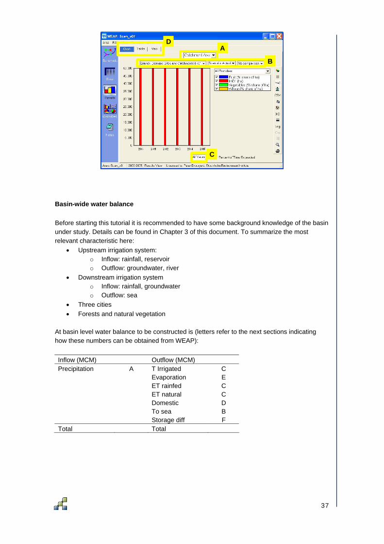
The Result screen might to be somewhat overwhelming at the first glance. WEAP offers an unlimited number of results that can be aggregated by years, months, scenarios, nodes, etc. Moreover, results can be presented as tables, graphs and maps. The following Figure shows where to start with the output analysis:
• A: main results selection with 6 main items, including various sub-selections • B: select all nodes or one or more specific nodes, and select scenario • C: select the period • D: output as graph, table or map. Normally graph output is good to start and chance to
table for exact numbers.
36
A
B
C
D
Basin-wide water balance
Before starting this tutorial it is recommended to have some background knowledge of the basin under study. Details can be found in Chapter 3 of this document. To summarize the most relevant characteristic here:
• Upstream irrigation system: o Inflow: rainfall, reservoir o Outflow: groundwater, river
• Downstream irrigation system o Inflow: rainfall, groundwater o Outflow: sea
• Three cities • Forests and natural vegetation
At basin level water balance to be constructed is (letters refer to the next sections indicating how these numbers can be obtained from WEAP): Inflow (MCM) Outflow (MCM) Precipitation A T Irrigated C Evaporation E ET rainfed C ET natural C Domestic D To sea B Storage diff F Total Total
37

A: Precipitation To obtain total available water at basin level, only rainfall is relevant as no inter-basin transfer takes place. The Figure below shows how to do this in the WEAP interface. This will be described in the context of this manual as:
Catchments > Observed Precipitation
To get the same results as numbers press the Table tab:
This Table shows that total rainfall, and thus total water availability at basin scale, is 21,600 MCM1 for the year 2005. This corresponds to what was provided as input for the model: 600 mm and 3,600,000 ha. B: Outflow to sea Next question to be answered is what happens with this 21,600 MCM. Part of it might flow out of the basin into the sea. There are two outflow points: waste water from City03 and outflow of the main river. Outflow from the river can be obtained by:
Supply and Resources > River > Streamflow > Below Catchment Inflow Node 6
1 MCM is Million Cubic Meter (106 m3)
38

To obtain outflow to the sea from City03:
Supply and Resources > Return Link > Flows
Using the Table tab one can see that for 2005 a total of 2,659 MCM flows into the sea of which the city only contributes 68.6 MCM. Notice that these return flows can be considered as real losses as reuse is not possible. C: Actual evapotranspiration Water is also consumed by vegetation (natural, rainfed and irrigated agriculture) and domestic use. In order to get the actual evapotranspiration of all vegetation one can use:
Catchments > ETActual
Interesting is that most evapotranspiration occurs at the Catch01 to Catch04, and is thus natural vegetation and some rainfed crops. Using the Level option and setting this at 2 one can get the distribution for the various vegetation types. In the basin, most water is consumed by forests and shrublands.
39
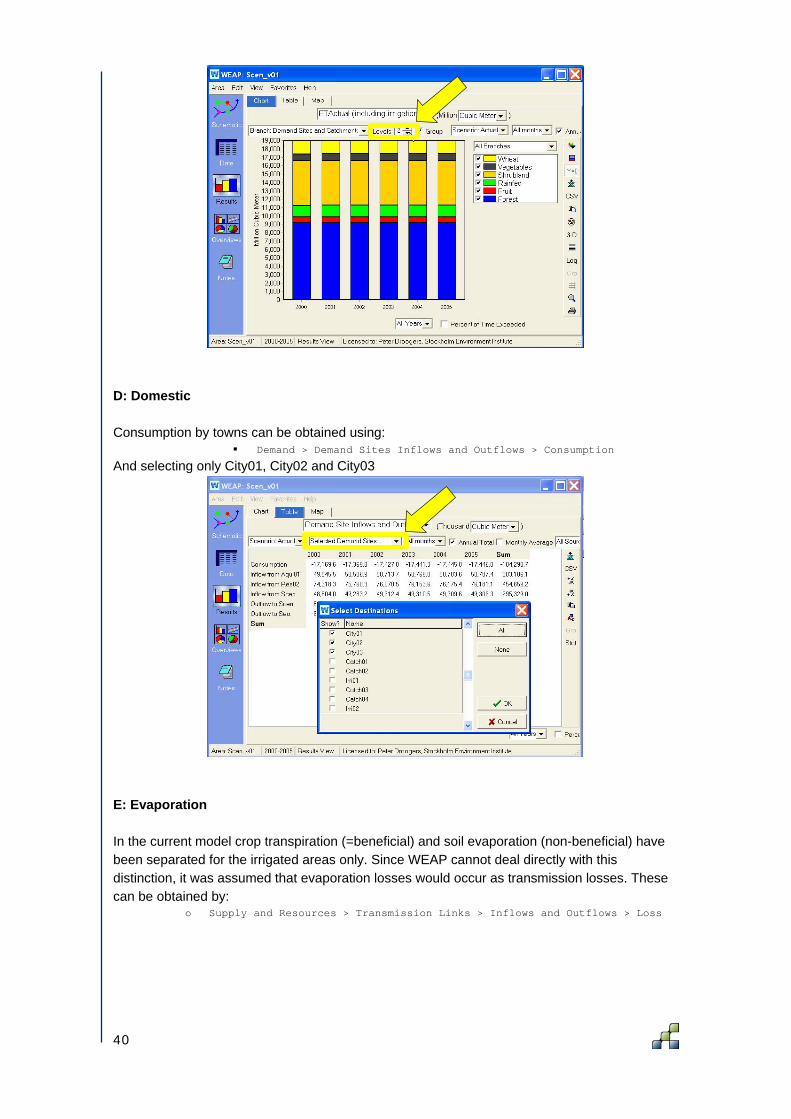
D: Domestic Consumption by towns can be obtained using:
Demand > Demand Sites Inflows and Outflows > Consumption
And selecting only City01, City02 and City03
E: Evaporation In the current model crop transpiration (=beneficial) and soil evaporation (non-beneficial) have been separated for the irrigated areas only. Since WEAP cannot deal directly with this distinction, it was assumed that evaporation losses would occur as transmission losses. These can be obtained by:
o Supply and Resources > Transmission Links > Inflows and Outflows > Loss
40

These evaporation losses are in total 840.7 MCM for the year 2005. F: Storage changes The last component to get the water balance closed is changes in storage for the aquifer and the reservoir over 2005. For the reservoir one should compare the reservoir levels of December 2004 with the levels of December 2005:
o Supply and Resources > Reservoir > Storage Volume.
It is clear that within a year huge difference between reservoir levels exist, but variation from year to year (Dec 2004 to Dec 2005) is negligible. The aquifer in the basin shows a substantial drop down over the years:
o Supply and Resources > Groundwater > Storage
41

Comparing December 2004 (3,346 MCM) to December 2005 (2,416 MCM) indicates that quite some water was withdrawn from the aquifer (930 MCM). Unmet demand Although not necessary for the water balance, it is good to know what the total water shortage is in the basin. WEAP is also able to provide this so-called unmet demand for the basin.
Demand > Unmet Demand
WEAP evaluates also the unmet demand for natural vegetation, defined as the actual minus the potential evapotranspiration. Obviously, this is something water managers cannot influence as this is a function of the precipitation. Note also that the unmet demand for cities is very low and for the two irrigated areas 700 and 3,300 MCM respectively. Basin water balance Based on the numbers collected the entire water balance from the basin can be constructed:
42
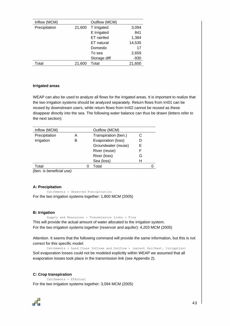
Inflow (MCM) Outflow (MCM) Precipitation 21,600 T Irrigated 3,094 E Irrigated 841 ET rainfed 1,384 ET natural 14,535 Domestic 17 To sea 2,659 Storage diff -930Total 21,600 Total 21,600
Irrigated areas
WEAP can also be used to analyze all flows for the irrigated areas. It is important to realize that the two irrigation systems should be analyzed separately. Return flows from Irri01 can be reused by downstream users, while return flows from Irri02 cannot be reused as these disappear directly into the sea. The following water balance can thus be drawn (letters refer to the next section): Inflow (MCM) Outflow (MCM) Precipitation A Transpiration (ben.) C Irrigation B Evaporation (loss) D Groundwater (reuse) E River (reuse) F River (loss) G Sea (loss) H Total 0 Total 0
(ben. is beneficial use) A: Precipitation
Catchments > Observed Precipitation
For the two irrigation systems together: 1,800 MCM (2005) B: Irrigation
Supply and Resources > Transmission Links > Flow
This will provide the actual amount of water allocated to the irrigation system. For the two irrigation systems together (reservoir and aquifer): 4,203 MCM (2005) Attention. It seems that the following command will provide the same information, but this is not correct for this specific model:
Catchments > Land Class Inflows and Outflow > (select Src/Dest. Irrigation)
Soil evaporation losses could not be modeled explicitly within WEAP we assumed that all evaporation losses took place in the transmission link (see Appendix 2). C: Crop transpiration
Catchments > ETActual
For the two irrigation systems together: 3,094 MCM (2005)
43
E: Evaporation
• Supply and Resources > Transmission Links > Inflows and Outflows > Loss
For the two irrigation systems together: 841 MCM (2005) F: Groundwater
• Catchments > Infiltration/Runoff Flow
Flows to the groundwater occur only from Irri01. Note that these flows cannot be considered as losses, as these are reused by downstream users. H: Outflow to river
Catchments > Infiltration/Runoff Flow
Outflow to the river should be sometimes considered as reusable flows (upstream system) and sometimes as real losses (downstream system). Unmet demand
Catchments > ETshortfall
Total unmet demand (shortage) for the two systems is 1,982 MCM. Irrigation system water balance Based on the numbers collected above, the water balance for the two irrigation systems can be constructed: Inflow (MCM) Outflow (MCM) Precipitation 1,800 Transpiration (ben.) 3,094Irrigation (surfacew) 2,191 Evaporation (loss) 841Irrigation (groundw) 2,012 Groundwater (reuse) 97 Drainage (reuse) 227 Drainage (loss) 1,744 Total 6,003 Total 6,003
It is important to treat the component of the outflow differently:
• beneficial outflow: crop transpiration • non-beneficial outflow: soil evaporation, drainage (downstream) • reusable outflow: percolation (upstream), drainage (upstream)
Only based on this classification water managers and policy makers can make the appropriate choice of where to improve water management.
44

-125
-100
-75
-50
-25
0
25
50
75
100
125
Rel
ativ
e Fl
ows
(%)
Precipitation
Irrigation
Transpiration
Soil evaporationGroundwater recharge
Runoff
Upstream Downstream
Transpiration
Evaporation
Groundwater
Drainage
Transpiration
Evaporation
Drainage
Irr01
Irr02
45
Appendix 2: WEAP Tips and Tricks Soil evaporation losses It is highly recommended to make a clear distinction between crop transpiration and soil evaporation. The first one can be considered as beneficial, since vegetation growth is a function of crop transpiration. In contrast to this is soil evaporation which is an non-beneficial loss of water. Given the nature of the WEAP model, this distinction between crop transpiration and soil evaporation can not be made. More physical based models, such as SWAP and SWAT, can deal with this but are at the same time much more data demanding and more complex to do scenario analysis. In order to make the distinction between beneficial crop transpiration and non-beneficial soil evaporation in WEAP the following procedure can be applied.
• The Transmission link (irrigation canal) is considered as an integrated part of the entire Catchment (irrigation system).
• In a Transmission link losses from the system can be defined as percentage of the flow: o WEAP > Data > Supply and Resources > Linking Demands and Supply > to
Irr01 > from Res01 > Loss from System
• To get the output of these evaporation losses: o WEAP > Results > Supply and Resources > Transmission Links > Inflows and
Outflows > Loss
or: o WEAP > Data > Supply and Resources > Outflows from Areas > Transmission
Link from Res01 to Irri01
Note that this approach is somewhat static and assumes only that a percentage of the incoming flow is lost by soil evaporation and ignores soil evaporation from rainfall. Irrigation Efficiency The classical term “irrigation efficiency” can be implemented in WEAP in various ways. The first option is to assume that percolation will be explicitly defined, using
• In a Transmission link percolation to groundwater can be defined as percentage of the flow:
o WEAP > Data > Supply and Resources > Linking Demands and Supply > to Irr01 > from Res01 > Loss to Groundwater
Note that the term “loss” is not completely correct in this respect as water percolates to the groundwater and might be reused. A somewhat better option to use is the Irrigation Fraction as the water not used for evapotranspiration will flow to the groundwater and/or surface water.
WEAP > Data > Demand Sites and Catchments > Irri01 > Irrigation Fraction
The distribution of water flowing to the groundwater and to the surface water is defined in o WEAP > Data > Supply and Resources > Runoff and Infiltration > from
Irri01 > Runoff Fraction
46

Non trivial output In WEAP some of the results that can be obtained for Catchments might be confusing. Here is a list of output that should be handled with care:
• Inflows to Area. For Catchments this means only precipitation: WEAP > Result > Supply and Resources > Inflows to Area
Same result can be obtained by: WEAP > Result > Catchments > Observed Precipitation
• Outflow from Area. For City this means the actual consumption. To get the inflow,
consumption and outflow use: WEAP > Result > Demand Site > Demand Site Inflows and Outflows
Same result can be obtained by: WEAP > Result > Supply and Resources > Return Link > Flows
47