scaling, wavelets, image compression, and encoding - …msong/research/julia.pdf · scaling,...
TRANSCRIPT
Scaling, wavelets, image compression, andencoding
Palle E. T. Jorgensen and Myung-Sin Song
Abstract In this paper we develop a family of multi-scale algorithms with the useof filter functions in higher dimension.
While our primary application is to images, i.e., processesin two dimensions, weprove our theorems in a more general context, allowing dimension 3 and higher.
The key tool for our algorithms is the use of tensor products of representationsof certain algebras, the Cuntz algebrasON , from the theory of algebras of operatorsin Hilbert space. Our main result offers a matrix algorithm for computing coeffi-cients for images or signals in specific resolution subspaces. A special feature withour matrix operations is that they involve products and iteration of slanted matrices.Slanted matrices, while large, have many zeros, i.e., are sparse. We prove that as theoperations increase the degree of sparseness of the matrices increase. As a result,only a few terms in the expansions will be needed for achieving a good approxi-mation to the image which is being processed. Our expansionsare local in a strongsense.
An additional advantage with the use of representations of the algebrasON, andtensor products is that we get easy formulas for generating all the choices of matri-ces going into our algorithms.
1 Introduction
The paper is organized as follows: first motivation, history, and discussion of ourapplications. Since a number of our techniques use operatortheory, we have a sepa-
Palle E. T. JorgensenDepartment of Mathematics, The University of Iowa, Iowa City, IA52242, USA e-mail:[email protected]
Myung-Sin SongDepartment of Mathematics and Statistics, Southern Illinois University Edwardsville, Ed-wardsville, IL62026, USA e-mail:[email protected]
1
2 Palle E. T. Jorgensen and Myung-Sin Song
rate section with these results. We feel they are of independent interest, but we havedeveloped them here tailored to use for image processing.
A key tool in our algorithms is the use of slanted matrices, and tensor productsof representations. This material receives separate sections. The significance of theslanted property is that matrix products of slanted matrices become increasinglymore sparse (i.e., the resulting matrices have wide patterns of zeros) which makescomputations fast.
Motivation and Applications. We consider interconnections between three sub-jects which are not customarily thought to have much to do with one another: (1) thetheory of stochastic processes, (2) wavelets, and (3) sub-band filters (in the sense ofsignal processing).
While connections between (2) and (3) have gained recent prominence, see forexample [9], applications of these ideas to stochastic integration is of more recentvintage. Nonetheless, there is always an element of noise inthe processing of signalswith systems of filters. But this has not yet been modeled withstochastic processes,and it hasn’t previously been clear which processes do the best job.
Recall however that the notion of low-pass and high-pass filters derives in partfrom probability theory. Here high and low refers to frequency bands, but there maywell be more than two bands (not just high and low, but a finite range of bands). Theidea behind this is that signals can be decomposed accordingto their frequencies,with each term in the decomposition corresponding to a rangeof a chosen frequencyinterval, for example high and low. Sub-band filtering amounts to an assignment offilter functions which accomplish this: each of the filters will then block signalsin one band, and passes the others. This is known to allow for transmission of thesignal over a medium, for example wireless. It was discovered recently (see [9]),perhaps surprisingly, that the functions which give good filters in this context servea different purpose as well: they offer the parameters whichaccount for families ofwavelet bases, for example families of bases functions in the Hilbert spaceL2(R).Indeed the simplest quadrature-mirror filter is known to produce the Haar waveletbasis inL2(R).
It is further shown in [9] that both principles (2) and (3) aregoverned by fami-lies of representations of one of the Cuntz algebrasON, with the numberN in thesubscript equal to the number of sub-bands in the particularmodel. So for the Haarcase,N = 2.
A main purpose in this paper is pointing out that fractional Brownian motion(fBm) may be understood with the data in (2) and (3), and as a result that fBmmay be understood with the use of a family of representationsof ON; albeit a quitedifferent family of representations from those used in [9].
A second purpose we wish to accomplish is to show that the operators and rep-resentations we use in one dimension can be put together in a tensor product con-struction and then account for those filters which allow for processing of digitalimages. Here we think of both black and white, in which case wewill be using asingle matrix of pixel numbers. In the case of color images, the same idea applies,but then we will rather be using three matrices accounting for exposure of each ofthe three primary colors. If one particular family F of representations of one of the
Scaling, wavelets, image compression, and encoding 3
Cuntz algebrasON is used in 1D, then for 2D (images) we show that the relevantfamilies of representations ofON are obtained fromF with the use of tensor productof pairs of representations, each one chosen fromF .
1.1 Interdisciplinary dimensions
While there is a variety of interdisciplinary dimensions, math (harmonic, numerical,functional, ... ), computer science, engineering, physics, image science, we will offersome pointers here some pointers to engineering, signal andimage processing.
Engineering departments teach courses in digital images, as witnessed by suchstandard texts as [11]. Since 1997, there was a separate track of advances involvingcolor images and wireless communication, the color appearance of surfaces in theworld as a property that allows us to identify objects, see e.g., [17, 29], and [8, 7, 30].
From statistical inference we mention [28]. Color imaging devices such as scan-ners, cameras, and printers, see [26]. And on the more theoretical side, CS, [10].
2 History and Motivation
Here we discuss such tools from engineering as sub-band filters, and their manifoldvariations. They are ubiquitous in the processing of multi-scale data, such as arisesin wavelet expansions.
A powerful tool in the processing of signals or images, in fact going back tothe earliest algorithms, is that of subdividing the data into sub-bands of frequen-cies. In the simplest case of speech signals, this may involve a sub-division into thelow frequency range, and the high. An underlying assumptionfor this is that thedata admits such a selection of a totalfinite range for the set of all frequencies. Ifsuch a finite frequency interval can be chosen we talk about bandlimited analog sig-nals. Now depending of the choice of analysis and synthesis method to be used, thesuitability of bandlimited signals may vary. Shannon proved that once a frequencybandB has been chosen, then there is a Fourier representation for the signals, astime-series, with frequencies inB which allow reconstruction from a discrete set ofsamples in the time variable, sampled in an arithmetic progression at a suitable rate,the Nyquist rate. The theorem is commonly called the Shannonsampling theorem,and is also known as Nyquist—Shannon—Kotelnikov, Whittaker—Shannon, WKS,etc., sampling theorem, as well as the Cardinal Theorem of Interpolation Theory.
While this motivates a variety of later analogues to digital(A/D) tools, the currenttechniques have gone far beyond Fourier analysis.
Here we will focus on tools based on such multi-scale which are popular inwavelet analysis. But the basic idea of dividing the total space of data into sub-spaces corresponding to bands, typically frequency bands,will be preserved. Inpassing from speech to images, we will be aiming at the processes underlying the
4 Palle E. T. Jorgensen and Myung-Sin Song
processing of digital images, i.e., images arising as a matrix (or checkerboard) ofpixel numbers, or in case of color-images a linked system of three checkerboards,with the three representing the primary colors.
While finite or infinite families of nested subspaces are ubiquitous in mathemat-ics, and have been popular in Hilbert space theory for generations (at least since the1930s), this idea was revived in a different guise in 1986 by Stephane Mallat. It hassince found a variety of application to multiscale processes such as analysis on frac-tals. In its adaptation to wavelets, the idea is now referredto as the multiresolutionmethod.
What made the idea especially popular in the wavelet community was thatit offered a skeleton on which various discrete algorithms in applied mathematicscould be attached and turned into wavelet constructions in harmonic analysis. Infact what we now call multiresolutions have come to signify acrucial link betweenthe world of discrete wavelet algorithms, which are popularin computational math-ematics and in engineering (signal/image processing, datamining, etc.) on the oneside, and on the other side continuous wavelet bases in function spaces, especially inL2(Rd). Further, the multiresolution idea closely mimics how fractals are analyzedwith the use of finite function systems.
3 Operator Theory
Those key ideas multi-scale, wavelets, image processing, and the operator theoryinvolved discussed about, and used inside our paper are covered in a number of ref-erences. Especially relevant are the following [9, 3, 2, 4, 16, 19, 20, 21], but thereader will find additional important reference lists in thebooks [9] and [19]. A keyidea in the analysis we present here is to select a Hilbert space which will representthe total space of data; it may beL2(Rd) for a suitable chosend for dimension; orit may be anyone of a carefully selected closed subspaces. A representation of afunction ind variables into an expansion relative to an orthogonal basis(or a framebasis) corresponds to a subdivision of the total space into one-dimensional sub-spaces. But to get started one must typically select a fixed subspace which representa resolution of the data (or image) under consideration, then the further subdivisioninto closed subspaces can be accomplished with a scaling: The result is a family ofclosed subspaces, each representing a detail. There will then be a system of isome-tries which account for these subspaces, and there will be a scaling operation whichmakes (mathematically) precise the scale-similarity of the data in different detail-components of the total decomposition.
In wavelets, the scaling is by a number, for example 2, for dyadic wavelets. Inthis case, there will be two frequency bands. If the scale is instead by a positiveintegerN > 2, then there will beN natural frequency bands.
For images, or higher dimensional date, it is then natural touse an invertibled×dmatrix (over the integers), sayA, to model a choice of scaling. Scaling will then be
Scaling, wavelets, image compression, and encoding 5
modeled with powers ofA, i.e., withA j as j ranges over the integersZ. In this case,the number of frequency bands will beN := |det(A)|.
Here we review a harmonic analysis of isometries in Hilbert space. Our resultsare developed with view to applications to multi-scale processes. In the Hilbertspace framework, this takes the form of an exhaustion of closed subspaces, a mono-tone family of closed subspaces where one arises from the other by an applicationof a scaling operator.
But in mathematics, or more precisely in operator theory, the underlying ideadates back to work of John von Neumann, Norbert Wiener, and Herman Wold,where nested and closed subspaces in Hilbert space were usedextensively in anaxiomatic approach to stationary processes, especially for time series. Wold provedthat any (stationary) time series can be decomposed into twodifferent parts: Thefirst (deterministic) part can be exactly described by a linear combination of its ownpast, while the second part is the opposite extreme; it isunitary, in the language ofvon Neumann.
von Neumann’s version of the same theorem is a pillar in operator theory. Itstates that every isometry in a Hilbert spaceH is the unique sum of a shift isometryand a unitary operator, i.e., the initial Hilbert spaceH splits canonically as anorthogonal sum of two subspacesHs andHu in H , one which carries the shiftoperator, and the otherHu the unitary part. The shift isometry is defined from anested scale of closed spacesVn, such that the intersection of these spaces isHu.Specifically,
· · · ⊂V−1⊂V0⊂V1⊂V2⊂ ·· · ⊂Vn⊂Vn+1⊂ ·· ·∧
n
Vn = Hu, and∨
n
Vn = H .
However, Stephane Mallat was motivated by the notion of scales of resolutionsin the sense of optics. This in turn is based on a certain “artificial-intelligence”approach to vision and optics, developed earlier by David Marr at MIT, an approachwhich imitates the mechanism of vision in the human eye.
The connection from these developments in the 1980s back to von Neumannis this: Each of the closed subspacesVn corresponds to a level of resolution in such away that a larger subspace represents a finer resolution. Resolutions are relative, notabsolute! In this view, the relative complement of the smaller (or coarser) subspacein larger space then represents the visual detail which is added in passing from ablurred image to a finer one, i.e., to a finer visual resolution.
Subsequently, this view became popular in the wavelet community, as it of-fered a repository for the fundamental father and the motherfunctions, also calledthe scaling functionϕ , and the wavelet functionψ (see details below). Via a systemof translation and scaling operators, these functions thengenerate nested subspaces,and we recover the scaling identities which initialize the appropriate algorithms.This is now called the family of pyramid algorithms in wavelet analysis. The ap-proach itself is called the multiresolution approach (MRA)to wavelets. And in themeantime various generalizations (GMRAs) have emerged.
6 Palle E. T. Jorgensen and Myung-Sin Song
In all of this, there was a second “accident” at play: As it turned out, pyramidalgorithms in wavelet analysis now lend themselves via multiresolutions, or nestedscales of closed subspaces, to an analysis based on frequency bands. Here we referto bands of frequencies as they have already been used for a long time in signalprocessing.
One reason for the success in varied disciplines of the same geometric ideais perhaps that it is closely modeled on how we historically have represented num-bers in the positional number system. Analogies to the Euclidean algorithm seemespecially compelling.
3.0.1 Multiresolutions
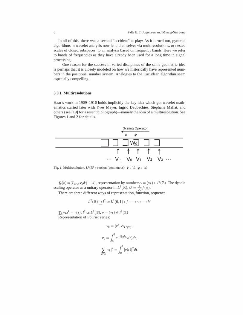
Haar’s work in 1909–1910 holds implicitly the key idea whichgot wavelet math-ematics started later with Yves Meyer, Ingrid Daubechies, Stephane Mallat, andothers (see [19] for a resent bibliograph)—namely the idea of a multiresolution. SeeFigures 1 and 2 for details.
W0
V-1 V0 V1 V2 V3
Scaling Operator
ψϕ
... ...
Fig. 1 Multiresolution.L2(Rd)-version (continuous);ϕ ∈V0, ψ ∈W0.
fv(x) = ∑k∈Z vkϕ(·−k), representation by numbersv= (vk)∈ l2(Z). The dyadicscaling operator as a unitary operator inL2(R), U = 1√
2f ( x
2).There are three different ways of representation, function, sequence
L2(R)⊃∼
l2 ≃ L2(0,1) : f ←→ v←→V
∑k vkzk = v(z), l2 ≃ L2(T), v = (vk) ∈ l2(Z)Representation of Fourier series:
vk = 〈zk,v〉L2(T),
vk =
∫ 1
0e−i2πktv(t)dt,
∑k∈Z
|vk|2 =
∫ 1
0|v(t)|2dt.
Scaling, wavelets, image compression, and encoding 7
Generating functions (engineering term):
H(z) = ∑k∈Z
hkzk wherez= ei2πt , andzk = ei2πkt
An equivalent form of the dyadic scaling operatorU in L2(R), U : Vϕ →Vϕ , soU restricts to an isometry in the subspaceVϕ .
(Uϕ)(x) =1√2
ϕ(x2)
=√
2∑j
h jϕ(x− j).
Setϕk = ϕ(·−k); then we have
(Uϕk)(x) =1√2
ϕk(x2)
=1√2
ϕ(x2−k)
=1√2
ϕ(x−2k
2)
=√
2∑j
h jϕ(x−2k− j)
=√
2∑j
h jϕ2k+ j .
It follows that
U ∑k
vkϕk =√
2∑l
∑k
vkh2k−l
=√
2∑l
h2k−l ϕ(x− l) if we let l = 2k− j.
As a result, we get:(MHv)l =
√2 ∑
k∈Z
h2k+lvk;
and(MHδp)l =
√2 ∑
k∈Z
h2k+lδp,k = h2p+l .
Lemma 1. Setting W: fv→∑k∈Z vkϕ(·−k) ∈Vϕ , and(S0 fv)(z) := H(z) fv(z2), wethen get the intertwining identity WS0 = UW on Vϕ .
Proof.
8 Palle E. T. Jorgensen and Myung-Sin Song
(WS0 fv)(x) = (W fS0v)(x)
= ∑k∈Z
(S0v)kϕ(x−k)
=1√2
∑k∈Z
vkϕ(x2−k)
=1√2
fv(x2) = (UW fv)(x).
Note that the isometryS0 = SH andS1 = SG areO2 Cuntz algebra.
√2
. . ....
......
· · · h2p−l h2p−l+2 · · ·· · · h2p−l−1 h2p−l+1 · · ·
......
.... . .
Sj0S1 are isometries forj = 0,1,2, · · · that generateO∞,
Q j = Sj0S1(S
j0S1)
∗ = Sj0S1S∗1S∗ j
0 =S1S∗1=1−S0S∗0
Sj0S∗ j
0Pj
−Sj+10 S∗ j+1
0Pj+1
,
n
∑j=0
Q j =n
∑j=0
(Pj −Pj+1) = I −Pn+1 →N→∞
I
sincePn+1 = Sn+1
0 S∗n+10 → 0 by pure isometry lemma in [19].
Recall an isometrySin a Hilbert spaceH is a shift if and only if limN→∞ SNS∗N =0. L2 is same as resolution space≃ Vϕ . The operators are as follows:Q0 = S1S∗1,Q1 = S0S1S∗1S∗0 = S0S1(S0S1)
∗. Note thatQ0 = I −P0, andQ j = Pj−Pj+1.ψ j ,k(x) = 2− j/2ψ(2− jx+k), j = 0,1,2, · · ·
∑∑c j ,kψ j ,k = ∑∑ fv(Q j v)k = ∑∑(Sj0S1S∗1S∗ j
0 v)kψ j ,k
If we now take the adjoint of these matrices, these correspond to the isometries.
S∗0∼M∗H ∼ F0,
S∗1 ∼M∗G∼ F1.
Theorem 1.The wavelet representation is given by slanted matrices as follows:∑∑(F1F j
0 v)kψ j ,k = fv
c j ,k = 〈ψ j ,k, f 〉=∫
ψ j ,k(x) f (x)dx.
· · · ⊂V−1⊂V0⊂V1⊂ ·· · , V0+W0 = V1.
Scaling, wavelets, image compression, and encoding 9
S0S1
S0...
S0S1
S0
S1... 2
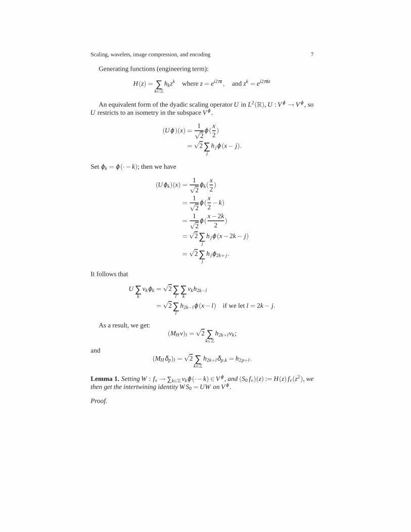
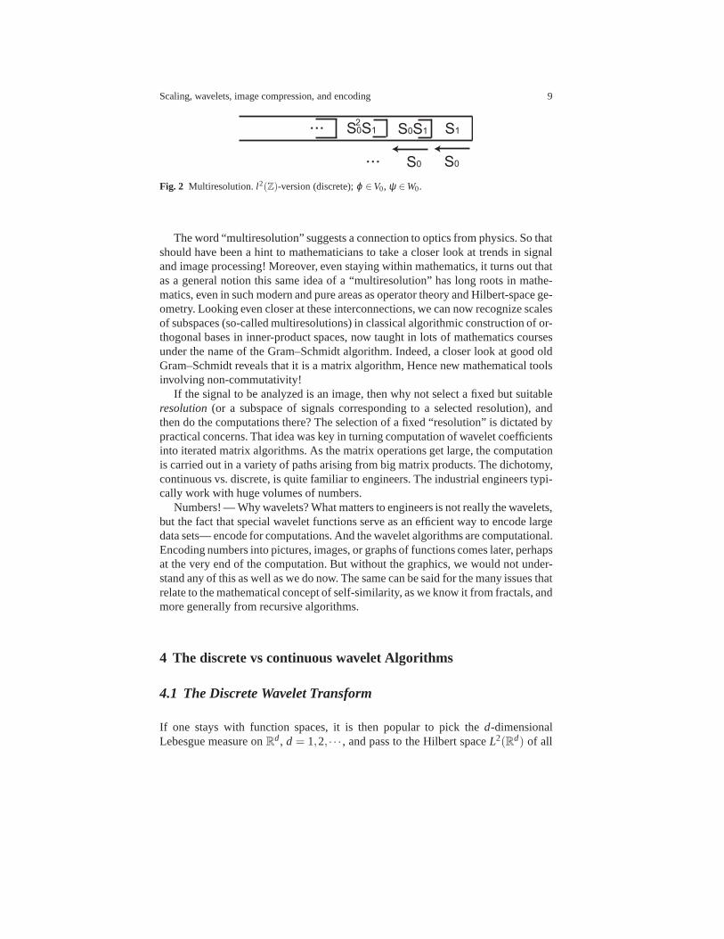
Fig. 2 Multiresolution.l2(Z)-version (discrete);ϕ ∈V0, ψ ∈W0.
The word “multiresolution” suggests a connection to opticsfrom physics. So thatshould have been a hint to mathematicians to take a closer look at trends in signaland image processing! Moreover, even staying within mathematics, it turns out thatas a general notion this same idea of a “multiresolution” haslong roots in mathe-matics, even in such modern and pure areas as operator theoryand Hilbert-space ge-ometry. Looking even closer at these interconnections, we can now recognize scalesof subspaces (so-called multiresolutions) in classical algorithmic construction of or-thogonal bases in inner-product spaces, now taught in lots of mathematics coursesunder the name of the Gram–Schmidt algorithm. Indeed, a closer look at good oldGram–Schmidt reveals that it is a matrix algorithm, Hence new mathematical toolsinvolving non-commutativity!
If the signal to be analyzed is an image, then why not select a fixed but suitableresolution(or a subspace of signals corresponding to a selected resolution), andthen do the computations there? The selection of a fixed “resolution” is dictated bypractical concerns. That idea was key in turning computation of wavelet coefficientsinto iterated matrix algorithms. As the matrix operations get large, the computationis carried out in a variety of paths arising from big matrix products. The dichotomy,continuous vs. discrete, is quite familiar to engineers. The industrial engineers typi-cally work with huge volumes of numbers.
Numbers! — Why wavelets? What matters to engineers is not really the wavelets,but the fact that special wavelet functions serve as an efficient way to encode largedata sets— encode for computations. And the wavelet algorithms are computational.Encoding numbers into pictures, images, or graphs of functions comes later, perhapsat the very end of the computation. But without the graphics,we would not under-stand any of this as well as we do now. The same can be said for the many issues thatrelate to the mathematical concept of self-similarity, as we know it from fractals, andmore generally from recursive algorithms.
4 The discrete vs continuous wavelet Algorithms
4.1 The Discrete Wavelet Transform
If one stays with function spaces, it is then popular to pick the d-dimensionalLebesgue measure onRd, d = 1,2, · · · , and pass to the Hilbert spaceL2(Rd) of all
10 Palle E. T. Jorgensen and Myung-Sin Song
square integrable functions onRd, referring to d-dimensional Lebesgue measure. Awavelet basis refers to a family of basis functions forL2(Rd) generated from a finiteset of normalized functionsψi , the indexi chosen from a fixed and finite index setI ,and from two operations, one called scaling, and the other translation. The scaling istypically specified by ad by d matrix over the integersZ such that all the eigenval-ues in modulus are bigger than one, lie outside the closed unit disk in the complexplane. Thed-lattice is denotedZd , and the translations will be by vectors selectedfrom Zd. We say that we have a wavelet basis if the triple indexed family
ψi, j ,k(x) := |detA| j/2ψ(A jx+k)
forms an orthonormal basis (ONB) forL2(Rd) as i varies inI , j ∈ Z, andk ∈ Rd.The word “orthonormal” for a familyF of vectors in a Hilbert spaceH refers tothe norm and the inner product inH : The vectors in an orthonormal family F areassumed to have norm one, and to be mutually orthogonal. If the family is also total(i.e., the vectors inF span a subspace which is dense inH ), we say thatF is anorthonormal basis (ONB.)
While there are other popular wavelet bases, for example frame bases, and dualbases (see e.g., [6, 15] and the papers cited there), the ONBsare the most agreeableat least from the mathematical point of view.
That there are bases of this kind is not at all clear, and the subject of wavelets inthis continuous context has gained much from its connections to the discrete worldof signal- and image processing.
Here we shall outline some of these connections with an emphasis on the math-ematical context. So we will be stressing the theory of Hilbert space, and boundedlinear operators acting in Hilbert spaceH , both individual operators, and familiesof operators which form algebras.
As was noticed recently the operators which specify particular subband algo-rithms from the discrete world of signal- processing turn out to satisfy relations thatwere found (or rediscovered independently) in the theory ofoperator algebras, andwhich go under the name of Cuntz algebras, denotedON if n is the number of bands.For additional details, see e.g., [19].
In symbols theC∗−algebra has generators(Si)N−1i=0 , and the relations are
N−1
∑i=0
SiS∗i = 1 (see Fig.3) (1)
(where1 is the identity element inON) and
N−1
∑i=0
SiS∗i = 1, andS∗i Sj = δi, j1. (2)
In a representation on a Hilbert space, sayH , the symbolsSi turn into boundedoperators, also denotedSi , and the identity element1 turns into the identity operatorI in H , i.e., the operatorI : h→ h, for h∈H . In operator language, the two formu-
Scaling, wavelets, image compression, and encoding 11
las 1 and 2 state that eachSi is an isometry inH , and that te respective rangesSiH
are mutually orthogonal, i.e.,SiH ⊥ SjH for i 6= j. Introducing the projectionsPi = SiS∗i , we getPiPj = δi, jPi , and
N−1
∑i=0
Pi = I .
Example 1.Fix N ∈ Z+. Then the easiest representation ofON is the following: LetH := l2(Z≥0), whereΓ := Z≥0 = {0}∪N = {0,1,2, · · ·}.
SetZN = {0,1, · · · ,N−1}= Z/NZ = the cyclic group of orderN.We shall denote canonical ONB inH = l2(Γ ) by |x〉 = δx with Dirac’s formal-
ism. Fori ∈ ZN setSi = ρ(si), given by
Si |x〉= |Nx+ i〉, x∈ Γ (3)
then
S∗i |x〉={| x−i
N 〉 if x− i ≡ 0 modN
0 otherwise.
The reader may easily verify the two relations in (2) by hand.For the use of Rep(ON,H ) in signal/image processing, more complicated for-
mulas than (3) are needed for the operatorsSi = ρ(si).
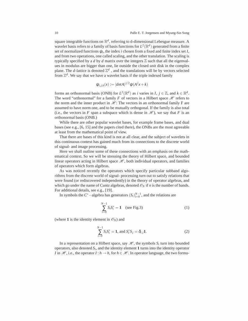
In the engineering literature this takes the form of programming diagrams:
Si*
Input Output
down-sampling up-sampling
Si
.
.
.
.
.
.
.
.
.
Fig. 3 Perfect reconstruction in a subband filtering as used in signal and image processing.
If the process of Figure 3 is repeated, we arrive at the discrete wavelet transformor stated in the form of images (n = 5)But to get successful subband filters, we must employ a more subtle family of
representations than those of (3) in Example 1. We now turn tothe study of thoserepresentations.
Selecting a resolution subspaceV0 = closure span{ϕ(·−k)|k∈ Z}, we arrive ata wavelet subdivision{ψ j ,k| j ≥ 0,k∈ Z}, whereψ j ,k(x) = 2 j/2ψ(2 jx−k), and the
12 Palle E. T. Jorgensen and Myung-Sin Song
first detail level
second detail level
third detail level
SH
SV SD
S0SDS0SV
S0SH
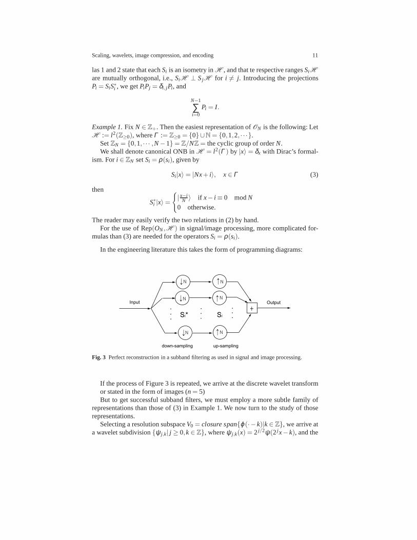
Fig. 4 The subdivided squares represent the use of the pyramid subdivision algorithm to imageprocessing, as it is used on pixel squares. At each subdivision step the top left-hand square repre-sents averages of nearby pixel numbers, averages taken withrespect to the chosen low-pass filter;while the three directions, horizontal, vertical, and diagonal represent detail differences, with thethree represented by separate bands and filters. So in this model, there are four bands, and theymay be realized by a tensor product construction applied to dyadic filters in the separate x- andthe y-directions in the plane. For the discrete WT used in image-processing, we use iteration offour isometriesS0,SH ,SV ,andSD with mutually orthogonal ranges, and satisfying the followingsum-ruleS0S∗0 +SHS∗H +SVS∗V +SDS∗D = I , with I denoting the identity operator in an appropriatel2-space.
continuous expansionf = ∑ j ,k〈ψ j ,k| f 〉ψ j ,k or the discrete analogue derived fromthe isometries,i = 1,2, · · · ,N−1,Sk
0Si for k = 0,1,2, · · · ; called the discrete wavelettransform.
Scaling, wavelets, image compression, and encoding 13
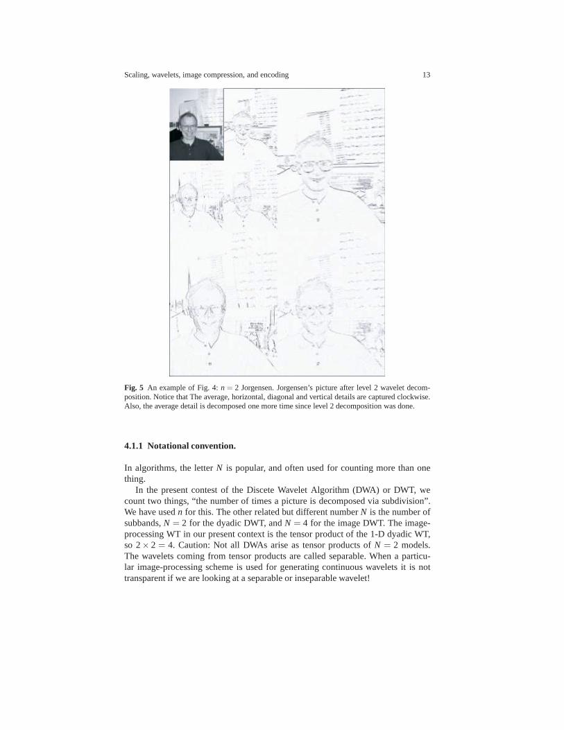
Fig. 5 An example of Fig. 4:n = 2 Jorgensen. Jorgensen’s picture after level 2 wavelet decom-position. Notice that The average, horizontal, diagonal and vertical details are captured clockwise.Also, the average detail is decomposed one more time since level 2 decomposition was done.
4.1.1 Notational convention.
In algorithms, the letterN is popular, and often used for counting more than onething.
In the present contest of the Discete Wavelet Algorithm (DWA) or DWT, wecount two things, “the number of times a picture is decomposed via subdivision”.We have usedn for this. The other related but different numberN is the number ofsubbands,N = 2 for the dyadic DWT, andN = 4 for the image DWT. The image-processing WT in our present context is the tensor product ofthe 1-D dyadic WT,so 2× 2 = 4. Caution: Not all DWAs arise as tensor products ofN = 2 models.The wavelets coming from tensor products are called separable. When a particu-lar image-processing scheme is used for generating continuous wavelets it is nottransparent if we are looking at a separable or inseparable wavelet!
14 Palle E. T. Jorgensen and Myung-Sin Song
To clarify the distinction, it is helpful to look at the representations of the Cuntzrelations by operators in Hilbert space. We are dealing withrepresentations of thetwo distinct algebrasO2, andO4; two frequency subbands vs 4 subbands. Notethat the CuntzO2, andO4 are given axiomatic, or purely symbolically. It is onlywhen subband filters are chosen that we get representations.This also means thatthe choice ofN is made initially; and the sameN is used in different runs of theprograms. In contrast, the number of times a picture is decomposed varies from oneexperiment to the next!
Summary: N = 2 for the dyadic DWT: The operators in the representation areS0
, S1. One average operator, and one detail operator. The detail operatorS1 “counts”local detail variations.
Image-processing. ThenN = 4 is fixed as we run different images in the DWT:The operators are now:S0, SH , SV , SD. One average operator, and three detail oper-ator for local detail variations in the three directions in the plane.
4.1.2 Increasing the dimension
In wavelet theory, [13] there is a tradition for reservingϕ for the father function andψ for the mother function. A 1-level wavelet transform of anN×M image can berepresented as
f 7→
a1 | h1
−− −−v1 | d1
(4)
where the subimagesh1,d1,a1 andv1 each have the dimension ofN/2 byM/2.
a1 = V1m⊗V1
n : ϕA(x,y) = ϕ(x)ϕ(y) = ∑i ∑ j hih jϕ(2x− i)ϕ(2y− j)h1 = V1
m⊗W1n : ψH(x,y) = ψ(x)ϕ(y) = ∑i ∑ j gih jϕ(2x− i)ϕ(2y− j)
v1 = W1m⊗V1
n : ψV(x,y) = ϕ(x)ψ(y) = ∑i ∑ j hig jϕ(2x− i)ϕ(2y− j)d1 = W1
m⊗W1n : ψD(x,y) = ψ(x)ψ(y) = ∑i ∑ j gig jϕ(2x− i)ϕ(2y− j)
(5)
whereϕ is the father function andψ is the mother function in sense of wavelet,V space denotes the average space and theW spaces are the difference space frommultiresolution analysis (MRA) [13].
We now introduce operatorsTH andTG in l2 such that the expression on the RHSin (5) becomesTH ⊗TH , TG⊗TH , TH ⊗TG andTG⊗TG, respectively.
We use the following representation of the two wavelet functionsϕ (father func-tion), andψ (mother function). A choice of filter coefficients(h j) and(g j) is made.
In the formulas, we have the following two indexed number systemsa := (hi)andd := (gi), a is for averages, andd is for local differences. They are really theinput for the DWT. But they also are the key link between the two transforms, thediscrete and continuous. The link is made up of the followingscaling identities:
Scaling, wavelets, image compression, and encoding 15
ϕ(x) = 2∑i∈Z
hiϕ(2x− i);
ψ(x) = 2∑i∈Z
giϕ(2x− i);
and (low-pass normalization)∑i∈Z hi = 1. The scalars(hi) may be real or complex;they may be finite or infinite in number. If there are four of them, it is called the “fourtap”, etc. The finite case is best for computations since it corresponds to compactlysupported functions. This means that the two functionsϕ andψ will vanish outsidesome finite interval on a real line.
The two number systems are further subjected to orthgonality relations, of which
∑i∈Z
hihi+2k =12
δ0,k (6)
is the best known.The systemsh and g are both low-pass and high-pass filter coefficients. In 5,
a1 denotes the first averaged image, which consists of average intensity values ofthe original image. Note that onlyϕ function,V space andh coefficients are usedhere. Similarly,h1 denotes the first detail image of horizontal components, whichconsists of intensity difference along the vertical axis ofthe original image. Notethatϕ function is used ony andψ function onx, W space forx values andV spacefor y values; and bothh andg coefficients are used accordingly. The datav1 denotesthe first detail image of vertical components, which consists of intensity differencealong the horizontal axis of the original image. Note thatϕ function is used onxandψ function ony, W space fory values andV space forx values; and bothhandg coefficients are used accordingly. Finally,d1 denotes the first detail image ofdiagonal components, which consists of intensity difference along the diagonal axisof the original image. The original image is reconstructed from the decomposedimage by taking the sum of the averaged image and the detail images and scaling bya scaling factor. It could be noted that onlyψ function,W space andg coefficientsare used here. See [37, 34].
This decomposition not only limits to one step but it can be done again and againon the averaged detail depending on the size of the image. Once it stops at certainlevel, quantization (see [33, 36]) is done on the image. Thisquantization step maybe lossy or lossless. Then the lossless entropy encoding is done on the decomposedand quantized image.
The relevance of the system of identities (6) may be summarized as follows. Set
m0(z) :=12 ∑
k∈Z
hkzk for all z∈ T;
gk := (−1)kh1−k for all k∈ Z;
m1(z) :=12 ∑
k∈Z
gkzk; and
16 Palle E. T. Jorgensen and Myung-Sin Song
(Sj f )(z) =√
2mj(z) f (z2), for j = 0,1, f ∈ L2(T), z∈ T.
Then the following conditions are equivalent:
(a)The system of equations (6) is satisfied.(b)The operatorsS0 andS1 satisfy the Cuntz relations.(c)We have perfect reconstruction in the subband system of Figure 3.
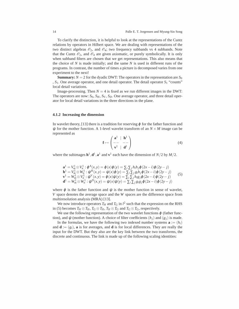
Note that the two operatorsS0 and S1 have equivalent matrix representations.Recall that by Parseval’s formula we haveL2(T)≃ l2(Z). So representingS0 insteadas an∞×∞ matrix acting on column vectorsx = (x j) j∈Z we get
(S0x)i =√
2 ∑j∈Z
hi−2 jx j
and for the adjoint operatorF0 := S∗0, we get the matrix representation
(F0x)i =1√2
∑j∈Z
h j−2ix j
with the overbar signifying complex conjugation. This is computational significanceto the two matrix representations, both the matrix forS0, and forF0 := S∗0, is slanted.However, the slanting of one is the mirror-image of the other, i.e.,
S0 : S0* : . . . .
. .
.
.
. . .
.
.
.
. .
. . . .
4.1.3 Significance of slanting
The slanted matrix representations refers to the corresponding operators inL2. Ingeneral operators in Hilbert function spaces have many matrix representations, onefor each orthonormal basis (ONB), but here we are concerned with the ONB con-sisting of the Fourier frequencieszj , j ∈ Z. So in our matrix representations for theS operators and their adjoints we will be acting on column vectors, each infinitecolumn representing a vector in the sequence spacel2. A vector inl2 is said to be offinite size if it has only a finite set of non-zero entries.
It is the matrixF0 that is effective for iterated matrix computation. Reason:Whena column vectorx of a fixed size, say 2 s is multiplied, or acted on byF0, the result
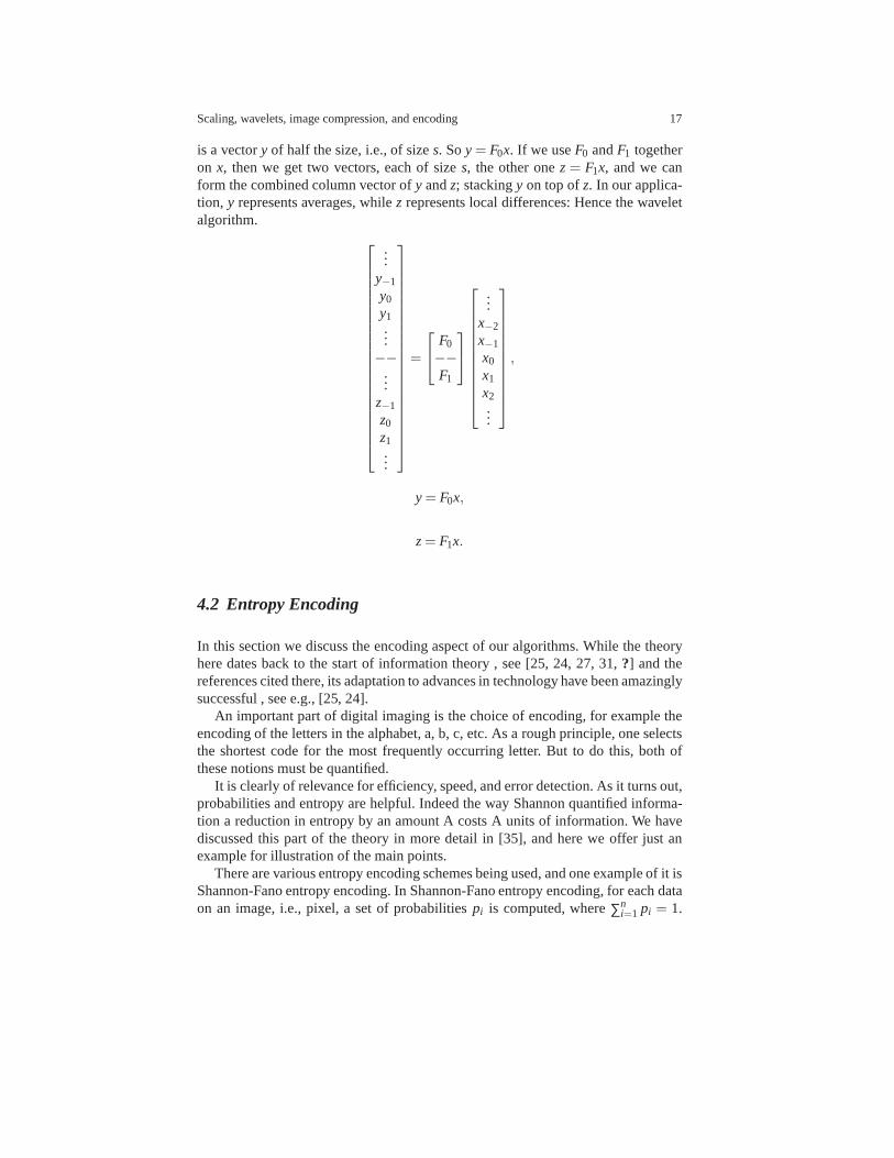
Scaling, wavelets, image compression, and encoding 17
is a vectory of half the size, i.e., of sizes. Soy = F0x. If we useF0 andF1 togetheron x, then we get two vectors, each of sizes, the other onez = F1x, and we canform the combined column vector ofy andz; stackingy on top ofz. In our applica-tion, y represents averages, whilez represents local differences: Hence the waveletalgorithm.
...y−1
y0
y1...−−
...z−1
z0
z1...
=
F0
−−F1
...x−2
x−1
x0
x1
x2...
,
y = F0x,
z= F1x.
4.2 Entropy Encoding
In this section we discuss the encoding aspect of our algorithms. While the theoryhere dates back to the start of information theory , see [25, 24, 27, 31,?] and thereferences cited there, its adaptation to advances in technology have been amazinglysuccessful , see e.g., [25, 24].
An important part of digital imaging is the choice of encoding, for example theencoding of the letters in the alphabet, a, b, c, etc. As a rough principle, one selectsthe shortest code for the most frequently occurring letter.But to do this, both ofthese notions must be quantified.
It is clearly of relevance for efficiency, speed, and error detection. As it turns out,probabilities and entropy are helpful. Indeed the way Shannon quantified informa-tion a reduction in entropy by an amount A costs A units of information. We havediscussed this part of the theory in more detail in [35], and here we offer just anexample for illustration of the main points.
There are various entropy encoding schemes being used, and one example of it isShannon-Fano entropy encoding. In Shannon-Fano entropy encoding, for each dataon an image, i.e., pixel, a set of probabilitiespi is computed, where∑n
i=1 pi = 1.
18 Palle E. T. Jorgensen and Myung-Sin Song
The entropy of this set gives the measure of how much choice isinvolved, in theselection of the pixel value of average.
Definition 1. Shannon’s entropyE(p1, p2, . . . , pn) which satisfy the following:
• E is a continuous function ofpi .• E should be steadily increasing function ofn.• If the choice is made ink successive stages, thenE = sum of the entropies of
choices at each stage, with weights corresponding to the probabilities of thestages.
E = −k∑ni=1 pi logpi . k controls the units of the entropy, which is ”bits.” logs are
taken base 2. [5, 32]
Shannon-Fano entropy encoding is done according to the probabilities of dataand the method is as follows:
• The data is listed with their probabilities in decreasing order of their probabilities.• The list is divided into two parts that has roughly equal probability.• Start the code for those data in the first part with a 0 bit and for those in the
second part with a 1.• Continue recursively until each subdivision contains justone data. [5, 32]
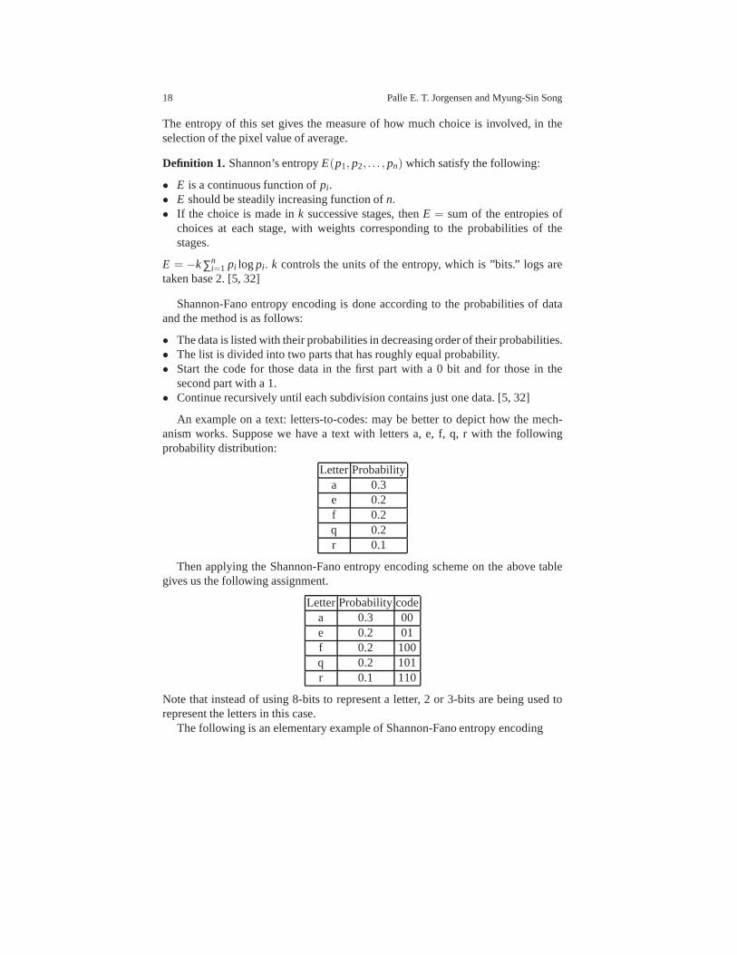
An example on a text: letters-to-codes: may be better to depict how the mech-anism works. Suppose we have a text with letters a, e, f, q, r with the followingprobability distribution:
LetterProbabilitya 0.3e 0.2f 0.2q 0.2r 0.1
Then applying the Shannon-Fano entropy encoding scheme on the above tablegives us the following assignment.
LetterProbabilitycodea 0.3 00e 0.2 01f 0.2 100q 0.2 101r 0.1 110
Note that instead of using 8-bits to represent a letter, 2 or 3-bits are being used torepresent the letters in this case.
The following is an elementary example of Shannon-Fano entropy encoding
Scaling, wavelets, image compression, and encoding 19
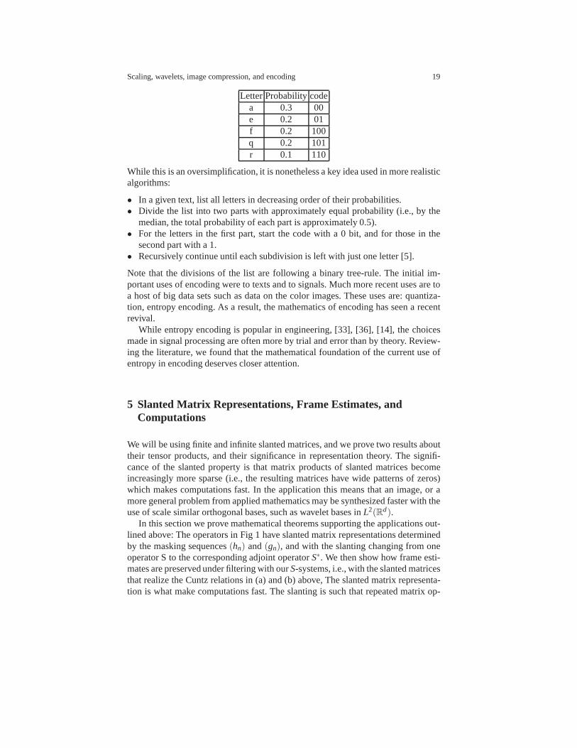
LetterProbabilitycodea 0.3 00e 0.2 01f 0.2 100q 0.2 101r 0.1 110
While this is an oversimplification, it is nonetheless a key idea used in more realisticalgorithms:
• In a given text, list all letters in decreasing order of theirprobabilities.• Divide the list into two parts with approximately equal probability (i.e., by the
median, the total probability of each part is approximately0.5).• For the letters in the first part, start the code with a 0 bit, and for those in the
second part with a 1.• Recursively continue until each subdivision is left with just one letter [5].
Note that the divisions of the list are following a binary tree-rule. The initial im-portant uses of encoding were to texts and to signals. Much more recent uses are toa host of big data sets such as data on the color images. These uses are: quantiza-tion, entropy encoding. As a result, the mathematics of encoding has seen a recentrevival.
While entropy encoding is popular in engineering, [33], [36], [14], the choicesmade in signal processing are often more by trial and error than by theory. Review-ing the literature, we found that the mathematical foundation of the current use ofentropy in encoding deserves closer attention.
5 Slanted Matrix Representations, Frame Estimates, andComputations
We will be using finite and infinite slanted matrices, and we prove two results abouttheir tensor products, and their significance in representation theory. The signifi-cance of the slanted property is that matrix products of slanted matrices becomeincreasingly more sparse (i.e., the resulting matrices have wide patterns of zeros)which makes computations fast. In the application this means that an image, or amore general problem from applied mathematics may be synthesized faster with theuse of scale similar orthogonal bases, such as wavelet basesin L2(Rd).
In this section we prove mathematical theorems supporting the applications out-lined above: The operators in Fig 1 have slanted matrix representations determinedby the masking sequences(hn) and(gn), and with the slanting changing from oneoperator S to the corresponding adjoint operatorS∗. We then show how frame esti-mates are preserved under filtering with ourS-systems, i.e., with the slanted matricesthat realize the Cuntz relations in (a) and (b) above, The slanted matrix representa-tion is what make computations fast. The slanting is such that repeated matrix op-
20 Palle E. T. Jorgensen and Myung-Sin Song
erations in the processing make for more sparse matrices, and hence for a smallernumber of computational steps in digital program operations for image processing.
We begin by introducing the Cuntz operatorsS . The two operators come fromthe two masking sequences(hn) and(gn) , also called filter-coefficients, also calledlow-pass and high-pass filters.
Definition 2. If (hn)n∈Z is a double infinite sequence of complex numbers, i.e.,hn ∈C, for all n∈ Z; set
(S0x)(m) =√
2 ∑n∈Z
hm−2nx(n) (7)
and adjoint(S∗0x)(m) =
√2 ∑
n∈Z
hn−2mx(n); for all m∈ Z. (8)
Then
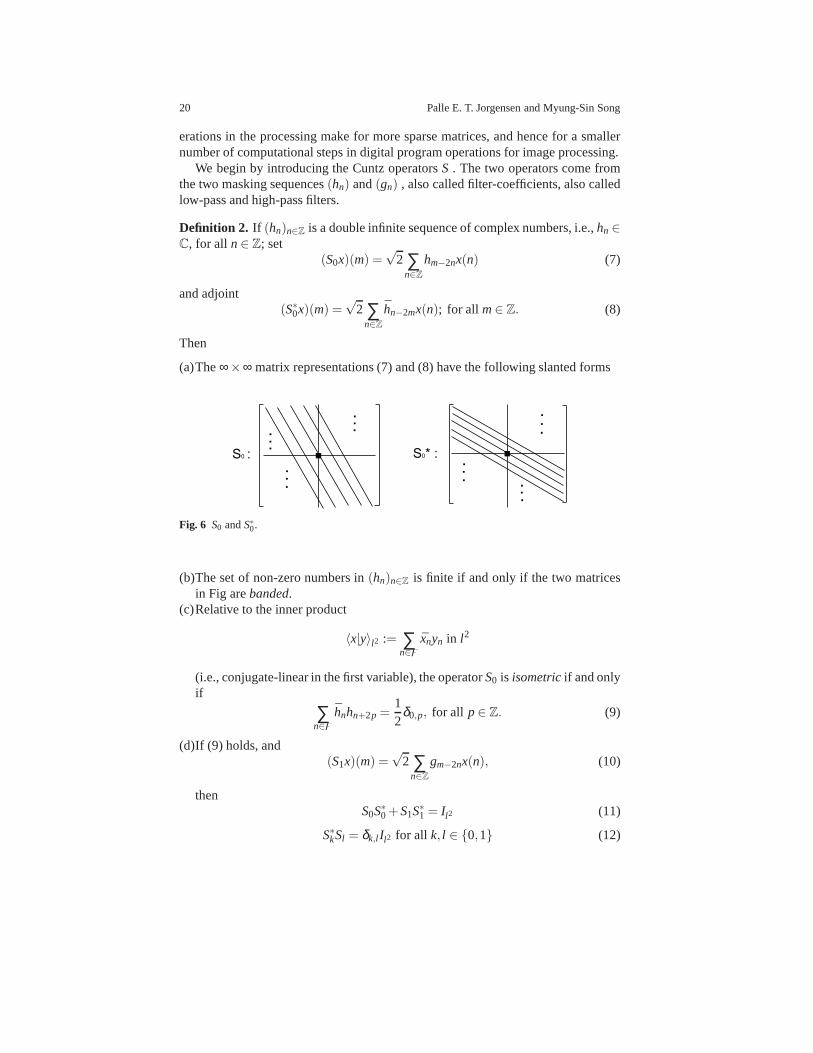
(a)The∞×∞ matrix representations (7) and (8) have the following slanted forms
S0 : S0* : . . . .
. .
.
.
. . .
.
.
.
. .
. . . .
Fig. 6 S0 andS∗0.
(b)The set of non-zero numbers in(hn)n∈Z is finite if and only if the two matricesin Fig arebanded.
(c)Relative to the inner product
〈x|y〉l2 := ∑n∈
xnyn in l2
(i.e., conjugate-linear in the first variable), the operator S0 is isometricif and onlyif
∑n∈
hnhn+2p =12
δ0,p, for all p∈ Z. (9)
(d)If (9) holds, and(S1x)(m) =
√2 ∑
n∈Z
gm−2nx(n), (10)
thenS0S∗0 +S1S∗1 = Il2 (11)
S∗kSl = δk,l Il2 for all k, l ∈ {0,1} (12)
Scaling, wavelets, image compression, and encoding 21
(the Cuntz relations) holds for
gn := (−1)ng1−n, n∈ Z.
Proof. By Parseval’s identity and Fourier transforms, we have theisometricisomor-phisml2(Z)≃ L2(T) whereT = {z∈C : |z|= 1} is equipped with Haar measure.
Hence the assertions (a)-(d) may be checked instead in the following functionrepresentation:
f (z) = ∑n∈
x(n)zn, (13)
m0(z) = ∑n∈
hnzn, (14)
m1(z) = ∑n∈
gnzn; (15)
setting
(Sj f )(z) = mj(z) f (z2), for all z∈ T, for all f ∈ L2(T), j = 0,1. (16)
In this form, the reader may check that conditions (a)-(d) are equivalent to the fol-lowing unitary principle: For almost everyz∈T (relative to Haar measure), we havethat the 2×2 matrix
U(z) =
(m0(z) m0(−z)m1(z) m1(−z)
)(17)
is unitary; i.e., thatU(z)∗ = U(z)−1, almost everyz∈ T, where(U∗)k,l := Ul ,k de-notes the adjoint matrix.
5.0.1 WARNING:
Note that the tensor product of two matrix-functions (17) does not have the sameform. Nonetheless, there is a more indirect way of creating new multiresolution-wavelet filters from old ones with the use of tensor-product;see details below.
SupposeA is an index set and(vα)α∈A ⊂ l2(Z) is a system of vectors subject tothe frame bound(B < ∞)
∑α∈A
|〈vα |x〉l2|2 ≤ B‖x‖2l2, for all x∈ l2. (18)
Setwj ,k := Sj
0S1vα , j ∈ N0 = {0,1,2, . . .},α ∈ A. (19)
If the unitarity condition (17) in the lemma is satisfied, then the induced system (19)satisfies the same frame bound (18).
Proof. Introducing Dirac’s notation for rank-one operators:
|u〉〈v||x〉= 〈v|x〉|u〉, (20)
22 Palle E. T. Jorgensen and Myung-Sin Song
we see that (18) is equivalent to the following operator estimate
∑α∈A
|vα〉〈vα | ≤ BIl2 (21)
where we use the standard ordering of the Hermitian operators, alias matrices.For the system(wj ,α )( j ,α)∈N0×A in (19), we therefore get
∑( j ,α)∈N0×A
|wj ,α〉〈wj ,α |= ∑j∑α
Sj0S1|vα〉〈vα |S∗1S∗ j
0
≤by(21)
B∑j
Sj0S1S∗1S∗ j
0 ≤ B,
Since
∑j
Sj0S1S∗1S∗
j
0 = I −Sn+10 S∗n+1
0 ≤ I for all n.
But the RHS in the last expression is the limit of the finite partial sums
N
∑j=0
Sj0S1S∗1S∗ j
0 =N
∑j=0
Sj0(I −S0S∗0)S
∗ j0 (22)
= Il2−SN+10 S∗
N+1
0 (23)
≤ Il2 since (24)
PN+1 := SN+10 S∗N+1
0 is a projection for allN ∈ N0. In fact
· · · ≤ PN+1≤ PN ≤ ·· · ≤ P1 = S0S∗0;
andP1 denotes the projection ontoS1l2.
5.0.2 Digital Image Compression
In [23], we showed that use of Karhunen-Loeve’s theorem enables us to pick thebest basis for encoding, thus to minimize the entropy and error, to better representan image for optimal storage or transmission. Here, optimalmeans it uses leastmemory space to represent the data; i.e., instead of using 16bits, use 11 bits. Sothe best basis found would allow us to better represent the digital image with lessstorage memory.
The particular orthonomal bases (ONBs) and frames which we use come fromthe operator theoretic context of the Karhunen-Loeve theorem [1]. In approximationproblems involving a stochastic component (for example noise removal in time-series or data resulting from image processing) one typically ends up with correla-tion kernels; in some cases as frame kernels.
Summary of the mathematics used in the various steps of the image compressionflow chart in Figure 3 (on next page):
Scaling, wavelets, image compression, and encoding 23
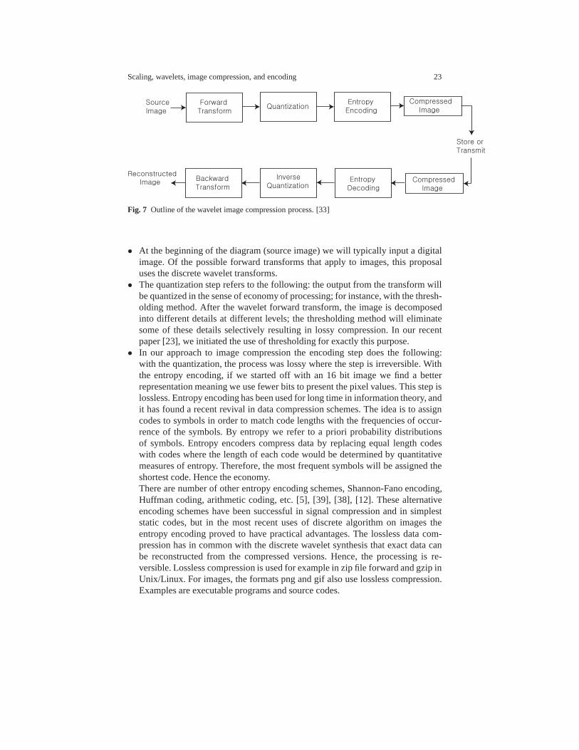
Fig. 7 Outline of the wavelet image compression process. [33]
• At the beginning of the diagram (source image) we will typically input a digitalimage. Of the possible forward transforms that apply to images, this proposaluses the discrete wavelet transforms.
• The quantization step refers to the following: the output from the transform willbe quantized in the sense of economy of processing; for instance, with the thresh-olding method. After the wavelet forward transform, the image is decomposedinto different details at different levels; the thresholding method will eliminatesome of these details selectively resulting in lossy compression. In our recentpaper [23], we initiated the use of thresholding for exactlythis purpose.
• In our approach to image compression the encoding step does the following:with the quantization, the process was lossy where the step is irreversible. Withthe entropy encoding, if we started off with an 16 bit image wefind a betterrepresentation meaning we use fewer bits to present the pixel values. This step islossless. Entropy encoding has been used for long time in information theory, andit has found a recent revival in data compression schemes. The idea is to assigncodes to symbols in order to match code lengths with the frequencies of occur-rence of the symbols. By entropy we refer to a priori probability distributionsof symbols. Entropy encoders compress data by replacing equal length codeswith codes where the length of each code would be determined by quantitativemeasures of entropy. Therefore, the most frequent symbols will be assigned theshortest code. Hence the economy.There are number of other entropy encoding schemes, Shannon-Fano encoding,Huffman coding, arithmetic coding, etc. [5], [39], [38], [12]. These alternativeencoding schemes have been successful in signal compression and in simpleststatic codes, but in the most recent uses of discrete algorithm on images theentropy encoding proved to have practical advantages. The lossless data com-pression has in common with the discrete wavelet synthesis that exact data canbe reconstructed from the compressed versions. Hence, the processing is re-versible. Lossless compression is used for example in zip file forward and gzip inUnix/Linux. For images, the formats png and gif also use lossless compression.Examples are executable programs and source codes.
24 Palle E. T. Jorgensen and Myung-Sin Song
In carrying out compression, one generates the statisticaloutput from the inputdata, and the next step maps the input data into bit-streams,achieving economyby mapping data into shorter output codes.
• The result of the three steps is the compressed information which could be storedin the memory or transmitted through internet. The technology in both ECW (En-hanced Compressed Wavelet technology) and JPEG2000 allow for fast loadingand display of large image files. JPEG2000 is wavelet-based image compression[19], [18]. There is a different brand new compressing scheme called EnhancedCompressed Wavelet technology (ECW). Both JPEG2000 and ECWare used inreconstruction as well.
5.1 Reconstruction
The methods described above apply to reconstruction questions from signal pro-cessing. Below we describe three important instances of this:
(i) In entropy decoding, the fewer bits assigned to represent the digital image aremapped back to the original number of bits without losing anyinformation.
(ii)In inverse quantization, there is not much of recovery to be obtained if threshold-ing was used for that was a lossy compression. For other quantization methods,this may yield some recovery.
(iii)The backward transform is the wavelet inverse transform where the decomposedimage is reconstructed back into an image that is of the same size as the originalimage in dimension but maybe of smaller size in memory.
LetT = R/Z≃{z∈C; |z|= 1}. LetA be ad×d matrix overZ such that‖λ‖> 1for all λ ∈ spec(A). Then the order of the groupA−1Zd/Zd is |detA| := N. ConsiderA−1Zd/Zd as a subgroup inTd = Rd/Zd.
We shall need the following bijection correspondence:
Definition 3. Forz∈ Td, zj = ei2πθ j , 1≤ j ≤ d, set
zA = (ei2πη j )d, (25)
whereAθ = η , (26)
i.e., ∑dj=1Ak jθ j = ηk, 1≤ k≤ d. Then forz∈ Td, the set{w ∈ Td;wA = z} is in
bijection correspondence with the finite groupA−1Zd/Zd.
Definition 4. LetUN(C) be the group of all unitaryN×N matrices, and letU AN (Td)
be the group of all measurable function
Td ∋ z 7→U(z) ∈UN(C). (27)
Let M AN (Td) be the multiresolution functions,
Scaling, wavelets, image compression, and encoding 25
Td ∋ z 7→M(z) = (mj(z))
N1 ∈C
N; (28)
i.e., satisfying1N ∑
w∈Td,wA=z
mj(w)mk(w) = δ j ,k. (29)
Example 2.Let{k j}Nj=1 be a selection of representatives for the groupZd/AZd; then
M0(z) = (zkj )Nj=1 (30)
is in M AN(Td).
Forz∈ Td andk∈ Zd we write
zk = (zk11 zk2
2 · · ·zkdd ) multinomial. (31)
Lemma 2. There is a bijection betweenU AN (Td) andM A
N (Td) given as follows:
(i) If u ∈U AN (Td) set
MU (z) = U(zA)M0(z) (32)
where M0 is the function in (30).(ii)If M ∈M A
N(Td), setUM(z) = (Ui, j(z))
Ni, j=1 (33)
with
Ui, j(z) =1N ∑
w∈Td,wA=z
M j(w)Mi(w). (34)
Proof. Case (i). GivenU ∈U AN (Td), we compute
1N ∑
wA=z
(MU )i(w)(MU) j(w) =by (32)
1N ∑
wA=z
(U(z)(wk)i(U(z)(wk) j
=1N ∑
wA=z
wki wkj
=1N ∑
wA=z
wkj−ki
= δi, j
where we have used the usual Fourier duality for the two finitegroups
A−1Z
d/Zd ≃ Z
d/AZd; (35)
i.e., a finite Fourier transform.Case (ii). GivenM ∈M A
N (Td), we computeUi, j(z) according to (34). The claimis thatU(z) = (Ui, j(z)) is in UN(C), i.e.,
26 Palle E. T. Jorgensen and Myung-Sin Song
N
∑l=1
Ul , j(z)Ul , j(z) = δi, j for all z∈ Td. (36)
Proof. Proof of (36):
N
∑l=1
Ul , j(z)Ul , j(z)
=by (34)
1N2 ∑
l∑w
∑w′
Mi(w)Ml (w)M j(w′)Ml (w′)
=1N ∑
w∑w′
δw,w′Mi(w)M j (w′)
=1N ∑
wMi(w)M j(w)
=by (30)
δi, j .
This completes the proof of (36) and therefore the Lemma. In the summations weconsider independent pairsw,w′ ∈ Td satisfyingwA = w′A = z. So each ranges overa set of cardinalityN = |detA|.
In the simplest case ofN = 2, d = 1, we have just two frequency bands, are twofilter functions
M =
(m0
m1
)
see (28), (29). In that case we select the two points±1 in bt. In additive notation,these represents the two elements in1
2Z/Z viewed as a subgroup ofT≃ R/Z. Theband-conditions are thenM0(1) = 1 andM1(−1) = 1, in addition notation:
Multi-band: high-pass/low-pass. IfN > 2, there will be more than two frequencybands. They can be written with the use of duality for the finite groupA−1Zd/Zd
in (36). Recall|detA| = N, and the group is cyclic of orderN. The matrix for itsFourier transform matrix is denotedHN with H Hadamard.
HN =1√N
(ei 2π jk
N
)
j ,k∈ZN
. (37)
Lemma 3. If U ∈ U AN (Td) and MU = U(zA)M0(z) is the multiresolution for the
lemma thenT
d ∋ z 7→HNMU(z) (38)
satisfying the multi-band frequency pass condition.
Proof. Immediate.
Lemma 4. Let M be a multi-band frequency pass function, see (38), and assumecontinuity at the zero-multi frequency, i.e., at the unit element inTd (with multi-plicative notation).
Scaling, wavelets, image compression, and encoding 27
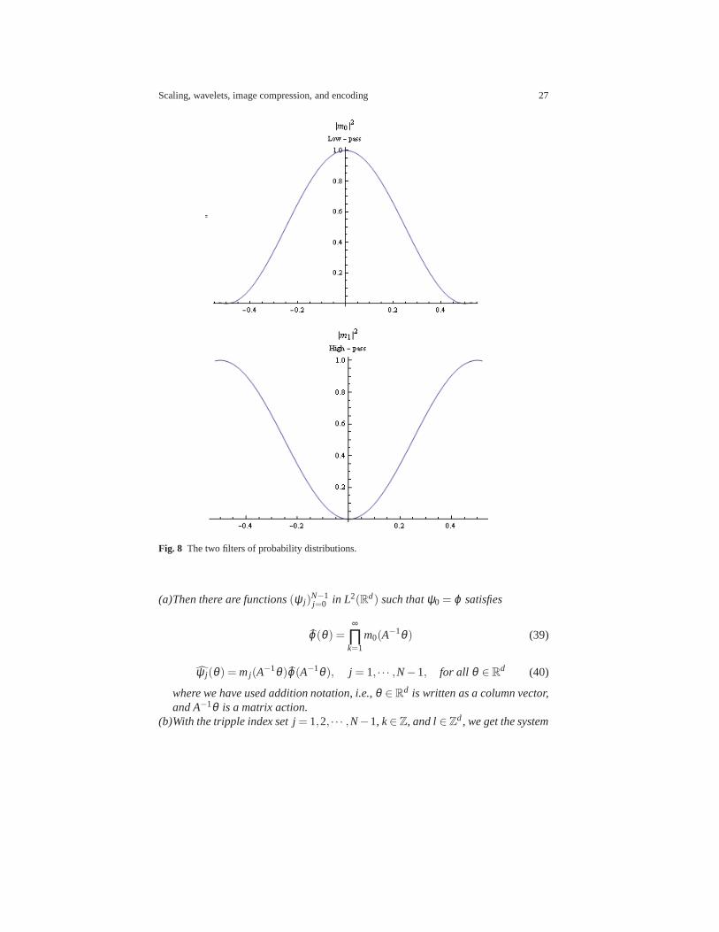
Fig. 8 The two filters of probability distributions.
(a)Then there are functions(ψ j)N−1j=0 in L2(Rd) such thatψ0 = ϕ satisfies
ϕ(θ ) =∞
∏k=1
m0(A−1θ ) (39)
ψ j(θ ) = mj(A−1θ )ϕ(A−1θ ), j = 1, · · · ,N−1, for all θ ∈R
d (40)
where we have used addition notation, i.e.,θ ∈Rd is written as a column vector,and A−1θ is a matrix action.
(b)With the tripple index set j= 1,2, · · · ,N−1, k∈ Z, and l∈Zd, we get the system
28 Palle E. T. Jorgensen and Myung-Sin Song
ψ j ,k,l (x) = |detA|k/2ψ j(Akx− l). (41)
(c)While the system in (41) in general does not form an orthonormal basis (ONB) inL2(Rd), it satisfies the following Parseval-fram condition: For every f ∈ L2(Rd),we have ∫
Rd| f (x)|2dx= ∑
1≤ j<N∑k∈Z
∑l∈Zd
|〈ψ j ,k,l , f 〉L2(Rd)|2 (42)
with the expression〈·, ·〉L2(Rd) on the RHS in (42) representing the usual L2(Rd)inner product
〈ψ , f 〉L2(Rd) =∫
Rdψ(x) f (x)dx. (43)
Proof. The essential idea is contained in [9], and the remaining details are left tothe reader.
Remark 1.The condition in (42) (Parseval-frame) is weaker than ONB, referring tofunction(ψ j ,k,l ) in (41). Rather thant asking for an ONB inL2(Rd), we seek insteada Parseval-frame. But there is a variety of explicit additional conditions on the givenwavelet filter from (39) and (40) which imply that(ψ j ,k,l ) is in fact an ONB.
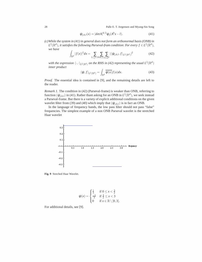
In the language of frequency bands, the low pass filter shouldnot pass “false”frequencies. The simplest example of a non ONB Parseval wavelet is the stretchedHaar wavelet
Fig. 9 Streched Haar Wavelet.
ψ(x) =
13 if 0 ≤ x < 3
2−13 if 3
2 ≤ x < 3
0 if x∈ R\ [0,3].
For additional details, see [9].
Scaling, wavelets, image compression, and encoding 29
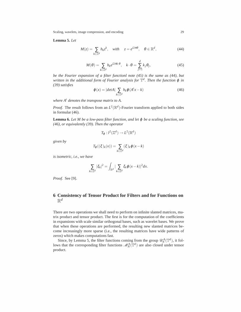
Lemma 5. Let
M(z) = ∑k∈Zd
hkzk, with z= ei2πθ , θ ∈ R
d, (44)
M(θ ) = ∑k∈Zd
hkei2πk·θ , k ·θ =
d
∑j=1
k jθ j , (45)
be the Fourier expansion of a filter functionl note (45) is thesame as (44), butwritten in the additional form of Fourier analysis forTd. Then the functionϕ in(39) satisfies
ϕ(x) = |detA| ∑k∈Zd
hkϕ(Atx−k) (46)
where At denotes the transpose matrix to A.
Proof. The result follows from anL2(Rd)-Fourier transform applied to both sidesin formular (46).
Lemma 6. Let M be a low-pass filter function, and letϕ be a scaling function, see(46), or equivalently (39). Then the operator
Tϕ : l2(Zd)→ L2(Rd)
given byTϕ((ξ )k(x)) = ∑
k∈Zd
(ξ )kϕ(x−k)
is isometric, i.e., we have
∑k∈Zd
|ξk|2 =
∫
Rd| ∑k∈Zd
ξkϕ(x−k)|2dx.
Proof. See [9].
6 Consistency of Tensor Product for Filters and for Functions onRd
There are two operations we shall need to perform on infinite slanted matrices, ma-trix product and tensor product. The first is for the computation of the coefficientsin expansions with scale similar orthogonal bases, such as wavelet bases. We provethat when these operations are performed, the resulting newslanted matrices be-come increasingly more sparse (i.e., the resulting matrices have wide patterns ofzeros) which makes computations fast.
Since, by Lemma 5, the filter functions coming from the groupU AN (Td), it fol-
lows that the corresponding filter functionsM AN(Td) are also closed under tensor
product.
30 Palle E. T. Jorgensen and Myung-Sin Song
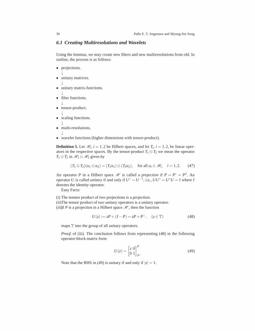
6.1 Creating Multiresolutions and Wavelets
Using the lemmas, we may create new filters and new multiresolutions from old. Inoutline, the process is as follows:
• projections.↓
• unitary matrices.↓
• unitary matrix-functions.↓
• filter functions.↓
• tensor-product.↓
• scaling functions.↓
• multi-resolutions.↓
• wavelet functions (higher dimensions with tensor-product).
Definition 5. Let Hi , i = 1,2 be Hilbert spaces, and letTi , i = 1,2, be linear oper-ators in the respective spaces. By the tensor-productT1⊗T2 we mean the operatorT1⊗T2 in H1⊗H2 given by
(T1⊗T2)(u1⊗u2) = (T1u1)⊗ (T2u2), for all ui ∈Hi , i = 1,2. (47)
An operatorP in a Hilbert spaceH is called aprojection if P = P∗ = P2. AnoperatorU is calledunitary if and only if U∗ = U−1, i.e.,UU∗ = U∗U = I whereIdenotes the identity operator.
Easy Facts:
(i) The tenstor product of two projections is a projection.(ii)The tensor product of two unitary operators is a unitaryoperator.(iii)If P is a projection in a Hilbert spaceH , then the function
U(z) := zP+(I −P) = zP+P⊥, (z∈ T) (48)
mapsT into the group of all unitary operators.
Proof. of (iii). The conclusion follows from representing (48) in the followingoperator-block matrix form
U(z) =
[z 00 1
]P
P⊥(49)
Note that the RHS in (49) is unitary if and only if|z|= 1.
Scaling, wavelets, image compression, and encoding 31
Definition 6. (1)LetA be ad×d matrix onbzsuch that spec(A)⊂{λ ∈C; |λ |> 1}.Let Zd πA→Zd/AZd =: QA be the natural quotient mapping. IfρA : Zd/AZd→ bzd
satisfyingπA◦ρA = id, we saw that
Td ∋ z 7→
(zρA(q)
)
q∈QA
is a multiresolution filter onTd.(2)If B is ae×ematric overZ such that spec(B)⊂ {λ ∈ C; |λ |> 1}, we introduce
QB = Ze/BZe andρB as in (1) by analogy. We then get ad + e multiresolutionfilter
Td×T
e∋ (z,w) 7→(
zρA(q)wρB(r))
q∈QA,r∈QB
.
(3)If NA := |detA|, andNB := |detB|, then the filter in (2) takes values inbcNA+NB.
Corollary 1. The families of multiresolution filtersM ANA
(Td) is closed under tensorproduct, i.e.,
MANA
(Td)⊗MBNB
(Te)⊂MA⊗BNA·NB
(Td+e).
Proof. By the lemma, we only need to observed that the unitary matrix-functionsTd ∋ z 7→UA(z) ∈UNA(C) are closed under tensor-product, i.e.,
Td⊗T
e∋ (z,w) 7→UA(z)⊗UB(w) ∈UNA·NB(C).
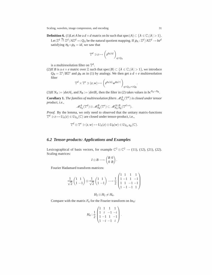
6.2 Tensor-products: Applications and Examples
Lexicographical of basis vectors, for exampleC2⊗C2 → (11), (12), (21), (22).Scaling matrices:
I ⊗B−→(
B 00 B
).
Fourier Hadamard transform matrices:
1√2
(1 11 −1
)⊗ 1√
2
(1 11 −1
)−→ 1
2
1 1 1 11 −1 1 −11 1 −1 −11 −1 −1 1
H2⊗H2 6= H4.
Compare with the matrixF4 for the Fourier transform onbz4:
H4 :12
1 1 1 11 i −1 −i1 −1 1 −11 −i −1 i
.
32 Palle E. T. Jorgensen and Myung-Sin Song
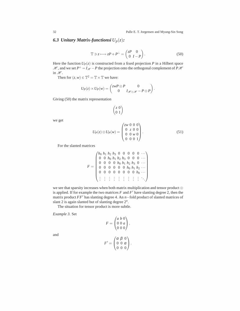
6.3 Unitary Matrix-functionsi Up(z):
T ∋ z 7−→ zP+P⊥ =
(zP 00 I −P
). (50)
Here the functionUP(z) is constructed from a fixed projectionP in a Hilbert spaceH , and we setP⊥= IH −P the projection onto the orthogonal complement ofPH
in H .Then for(z,w) ∈ T2 = T×T we have:
UP(z)×UP(w) =
(zwP⊗P 0
0 IH ⊗H −P⊗P
).
Giving (50) the matrix representation(
z 00 1
)
we get
UP(z)⊗UP(w) =
zw0 0 00 z 0 00 0 w 00 0 0 1
. (51)
For the slanted matrices
F =
h0 h1 h2 h3 0 0 0 0 0 · · ·0 0 h0 h1 h2 h3 0 0 0 · · ·0 0 0 0 h0 h1 h2 h3 0 · · ·0 0 0 0 0 0 h0 h1 h2 · · ·0 0 0 0 0 0 0 0h0 · · ·...
......
......
......
......
. . .
we see that sparsity increases when both matrix multiplication and tensor product⊗is applied. If for example the two matricesF andF ′ have slanting degree 2, then thematrix productFF ′ has slanting degree 4. Ann−fold product of slanted matrices ofslant 2 is again slanted but of slanting degree 2n.
The situation for tensor product is more subtle.
Example 3.Set
F =
a b 00 0 a0 0 0
,
and
F ′ =
α β 00 0 α0 0 0
.
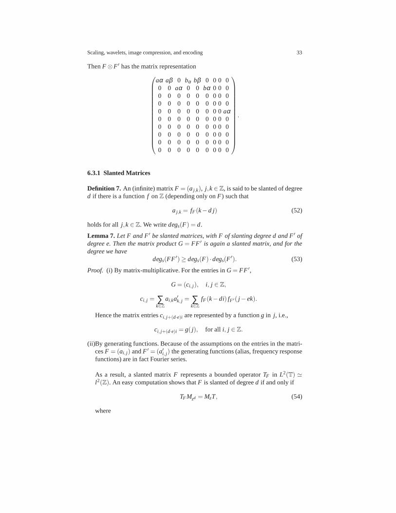
Scaling, wavelets, image compression, and encoding 33
ThenF⊗F ′ has the matrix representation
aα aβ 0 bα bβ 0 0 0 00 0 aα 0 0 bα 0 0 00 0 0 0 0 0 0 0 00 0 0 0 0 0 0 0 00 0 0 0 0 0 0 0aα0 0 0 0 0 0 0 0 00 0 0 0 0 0 0 0 00 0 0 0 0 0 0 0 00 0 0 0 0 0 0 0 00 0 0 0 0 0 0 0 0
.
6.3.1 Slanted Matrices
Definition 7. An (infinite) matrixF = (a j ,k), j,k∈ Z, is said to be slanted of degreed if there is a functionf onZ (depending only onF) such that
a j ,k = fF(k−d j) (52)
holds for all j,k∈ Z. We writedegs(F) = d.
Lemma 7. Let F and F′ be slanted matrices, with F of slanting degree d and F′ ofdegree e. Then the matrix product G= FF ′ is again a slanted matrix, and for thedegree we have
degs(FF ′)≥ degs(F) ·degs(F′). (53)
Proof. (i) By matrix-multiplicative. For the entries inG = FF ′,
G = (ci, j ), i, j ∈ Z,
ci, j = ∑k∈Z
ai,ka′k, j = ∑
k∈Z
fF(k−di) fF ′( j−ek).
Hence the matrix entriesci, j+(d·e)i are represented by a functiong in j, i.e.,
ci, j+(d·e)i = g( j), for all i, j ∈ Z.
(ii)By generating functions. Because of the assumptions onthe entries in the matri-cesF = (ai, j) andF ′ = (a′i, j) the generating functions (alias, frequency responsefunctions) are in fact Fourier series.
As a result, a slanted matrixF represents a bounded operatorTF in L2(T) ≃l2(Z). An easy computation shows thatF is slanted of degreed if and only if
TFMzd = MzT, (54)
where
34 Palle E. T. Jorgensen and Myung-Sin Song
(Mzξ )(z) = zξ (z), for all z∈ T;
and(Mzdξ )(z) = zdξ (z), ξ ∈ L2(T);
i.e.,Mzd = (Mz)d, d ∈ Z+.
As a result, we haveTFMzd = MzTF , and (55)
TF ′Mze = MzTF ′ . Since (56)
TG = TFTF ′ we get (57)
MzTG =by(57)
MzTFTF ′
=by(55)
TFMzdTF ′
=by(56)
TFTF ′M(zd)e
= TGMzd·e,
proving the assertion in the lemma.
The proof of the following result is analogous to that in Lemma 7 above.
Lemma 8. Let F and F′ be slanted matrices withZ as index set for rows andcolumns, or possibly subset ofZ. If degs(F) = d, and degs(F ′) = e, then F⊗F ′
is slanted relative to the index setZ2 by vector degree(d,e). Setting
(F⊗F ′)(i, j),(k,l) = Fi,kF′j ,l (58)
there is a function g onZ2 such that
(F⊗F ′)(i, j),(k,l) = g(k−di, l −e j) for all (i, j) ∈ Z2 and all (k, l) ∈ Z
2.
7 Rep(ON,H )
Here we show that the algorithms developed in the previous two sections may foundfrom certain representations of an algebra in a family indexed by a positive integerN, called the Cuntz algebrasON.
It will be important to make a distribution betweenON as aC∗-algebra, and itsrepresentation by operators in some Hilbert space. As we show distinct representa-tion of ON yield distinct algorithms, distinct wavelets, and distinct matrix computa-tions.
It is known thatON is the unique (up to isomorphism)C∗-algebra on generated(si)i ∈ ZN, and relations
Scaling, wavelets, image compression, and encoding 35
s∗i sj = δi, j1, ∑i∈ZN
sis∗i = 1. (59)
Heresi in (59) is a symbolic expression and 1 denotes the unit-element in theC∗-algebra generated by{si ; i ∈ZN}. Hence a representationρ of ON acting on a Hilbert
spaceH , ρ ∈ Rep(ON,H ), is a system of operatorsSi = S(ρ)i = ρ(si) satisfying
the same relations (59), but with 1 replaced byIH = ρ(1) = the identity operator inH .
From (59) it follows thatON⊗OM = ONM. Hence it follows from an analysis oftensor-product of representation that not all
ρ ∈ Rep(ON,H )
is a tensor product of a pair of representations, one ofON and the second ofOM.
References
1. Ash, R. B.Information Theory. Dover Publications Inc., New York, (1990) Corrected reprintof the 1965 original.
2. Aldroubi, A., Cabrelli, C., Hardin, D., Molter, U.: Optimal Shift Invariant Spaces and TheirParseval Frame Generators. Appl. Comput. Harmon. Anal.23, 2, 273–283 (2007)
3. Albeverio, S. and Jorgensen, P. E. T. and Paolucci, A. M. Multiresolution Wavelet Analysisof Integer Scale Bessel Functions.: J. Math. Phys.48, 7, 073516 (2007)
4. Ball, J. A. and Vinnikov, V.: Functional Models for representations of the Cuntz algebra. Op-erator theory, systems theory and scattering theory: multidimensional generalizations, Oper.Theory Adv. Appl.157, 1–60, Birkhauser, Basel (2005)
5. Cleary J. G. Witten I. H. Bell, T. C. Text Compression, Prentice Hall, Englewood Cliffs,(1990)
6. Baggett, L., Jorgensen, P. E. T., Merrill, K., Packer, J. Anon-MRA Cr frame wavelet withrapid decay.Acta Appl. Math., (2005)
7. Bose, T.,: Digital Signal and Image Processing, Wiley (2003)8. Bose, T., Chen, M.-Q., Thamvichai, R. Stability of the 2-DGivone-Roesser model with peri-
odic coefficients: IEEE Trans. Circuits Syst. I. Regul. Pap.54, 3, 566–578 (2007)9. Bratelli, O., Jorgensen, P. E. T.Wavelets Through a Looking Glass: The World of the Spec-
trum. Birkhauser, (2002)10. Burger, W.: Principles of Digital Image Processing: Fundamental Techniques, Springer
(2009)11. Burdick, H. E.: Digital Imaging: Theory and Applications, Mcgraw-Hill (1997)12. John G. Cleary, J. G., Witten, I. H. A comparison of enumerative and adaptive codes.IEEE
Trans. Inform. Theory, 30(2, part 2) 306–315, (1984)13. Daubechies, I.Ten lectures on wavelets, volume 61 ofCBMS-NSF Regional Conference
Series in Applied Mathematics. (1992)14. Donoho, D. L., Vetterli, M., DeVore, R. A., Daubechies, I. Data compression and harmonic
analysis.IEEE Trans. Inform. Theory, 44, 6, 2435–2476, (1998)15. Dutkay, D. E., Roysland, K. Covariant representations for matrix-valued transfer operators.
arXiv:math/0701453, (2007)16. Hutchinson, J. E.: Fractals and self-similarity. Indiana Univ. Math. J.30, 5, 713–747 (1981)17. Green, P., MacDonald, L.: Colour Engineering: Achieving Device Independent Colour, Wiley
(2002)
36 Palle E. T. Jorgensen and Myung-Sin Song
18. Jaffard, S., Meyer, Y., Ryan, R. D.Wavelets Tools for science & technology.. Society forIndustrial and Applied Mathematics (SIAM), Philadelphia,PA, revised edition, (2001)
19. Jorgensen, P. E. T.Analysis and probability: wavelets, signals, fractals, volume 234 ofGrad-uate Texts in Mathematics. Springer, New York, (2006)
20. Jorgensen, P. E. T., Kornelson, K., Shuman, K.: Harmonicanalysis of iterated function sys-tems with overlap. J. Math. Phys.48, 8, 083511 (2007)
21. Jorgensen, P. E. T., Mohari, A.: Localized bases inL2(0,1) and their use in the analysis ofBrownian motion. J. Approx. Theory151, 1, 20–41 (2008)
22. Jorgensen, P. E. T., Song, M.-S. Comparison of discrete and continuous wavelet transforms.Springer Encyclopedia of Complexity and Systems Science, (2007)
23. Jorgensen, P. E. T., Song, M.-S. Entropy encoding, hilbert space, and karhunen-loeve trans-forms. J. Math. Phys., 48, 10, 103503, (2007)
24. MacKay, D. J. C.: Information Theory, Inference and Learning Algorithms, Cambridge Uni-versity Press, New York, (2003)
25. Keyl, M.: Fundamentals of Quantum Information Theory, Phys. Rep.369, 5, 431–548, (2002)26. Rastislav L., Plataniotis, K. N.: Color Image Processing: Methods and Applications, CRC; 1
edition (2006)27. Roman, S.: Introduction to Coding and Information Theory: Undergraduate Texts in Mathe-
matics. Springer-Verlag, New York, (1997)28. Lukac, R., Plataniotis, K. N., Venetsanopoulos, A. N.: Bayer pattern demosaicking using
local-correlation approach. Computational science—ICCS2004. Part IV, Lecture Notes inComput. Sci.3039, 26–33, Berlin, Springer (2004)
29. MacDonald, L. (Editor), Luo, M. R. (Editor): Colour Image Science: Exploiting Digital Me-dia, Wiley; 1 edition (2002)
30. Russ, J. C.,The image processing handbook, 5th edn. (CRC Press, Boca Raton, FL, (2007)31. Salomon, D.: Data compression. The complete reference.4th edn. With contributions by Gio-
vanni Motta and David Bryant. Springer-Verlag, London, (2007)32. Shannon C.E., Weaver W.: The Mathematical Theory of Communication. University of Illi-
nois Press, Urbana and Chicago (1998)33. Skodras, A., Christopoulos, C., Ebrahimi, T. Jpeg 2000 still image compression standard”
ieee signal processing magazine.IEEE Signal processing Magazine, 18, 36–58, (2001)34. Song, M.-S. Wavelet image compression. InOperator theory, operator algebras, and appli-
cations, 414Contemp. Math., 41–73. Amer. Math. Soc., Providence, RI, (2006)35. Song, M.-S. Entropy encoding in wavelet image compression. Representations, Wavelets and
Frames A Celebration of the Mathematical Work of Lawrence Baggett, 293–311, (2008)36. Usevitch, B. E. A tutorial on modern lossy wavelet image compression: Foundations of jpeg
2000. IEEE Signal processing Magazine, 18, 22–35, (2001)37. Walker, J. S.A Primer on Wavelets and their Scientific Applications. Chapman & Hall, CRC,
(1999)38. Witten, I. H. Adaptive text mining: inferring structurefrom sequences.J. Discrete Algorithms,
2, 2, 137–159, (2004)39. Witten, I. H., Neal, R. M., Cleary, J. G. Arithmetic coding for data compression.Comm. of
the ACM, 30, 6, 520–540, (1987)