Scale Effects in Large Scale Watershed Modeling

Mustafa M. Aral and Orhan Gunduz

Multimedia Environmental Simulations LaboratorySchool of Civil and Environmental Engineering

Georgia Institute of TechnologyAtlanta, GA USA

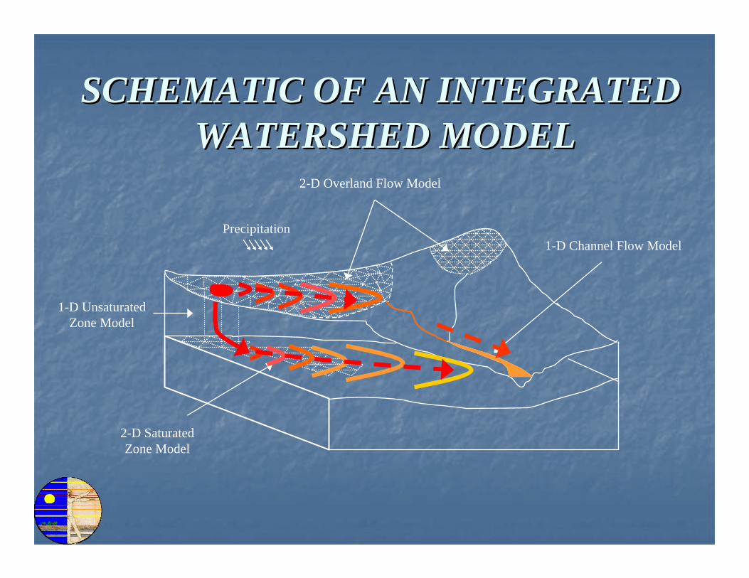
Precipitation

2-D Overland Flow Model

1-D Channel Flow Model

1-D UnsaturatedZone Model

2-D SaturatedZone Model

SCHEMATIC OF AN INTEGRATED SCHEMATIC OF AN INTEGRATED WATERSHED MODELWATERSHED MODEL

COMPLEXITIES.........COMPLEXITIES.........

MultiMulti--pathway flow and contaminant pathway flow and contaminant transport problem.transport problem.Integrated modeling of all pathways is the Integrated modeling of all pathways is the key.key.Each process pathway has its own Each process pathway has its own characteristic scale.characteristic scale.What should be the optimal scale of a What should be the optimal scale of a fully integrated model?fully integrated model?

MODELING TOOLSMODELING TOOLS

Lumped parameter modelsLumped parameter models

Distributed parameter modelsDistributed parameter models

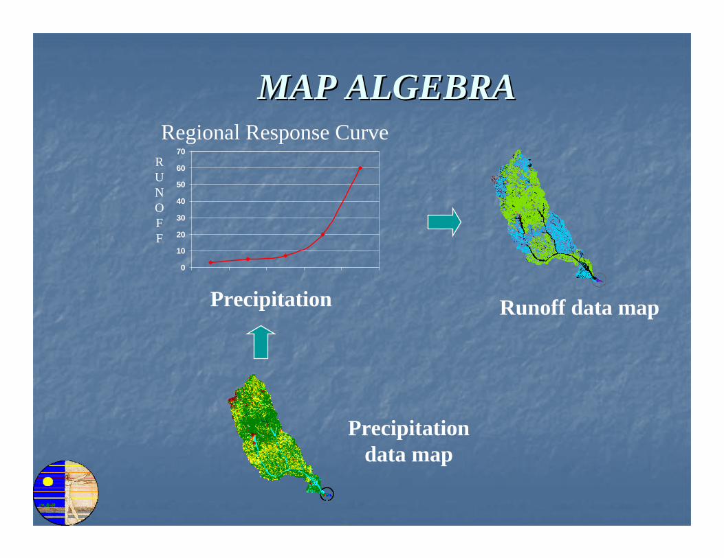
MAP ALGEBRAMAP ALGEBRA

Precipitation data map

Runoff data map

0

10

20

30

40

50

60

70

Precipitation

RUNOFF

Regional Response Curve

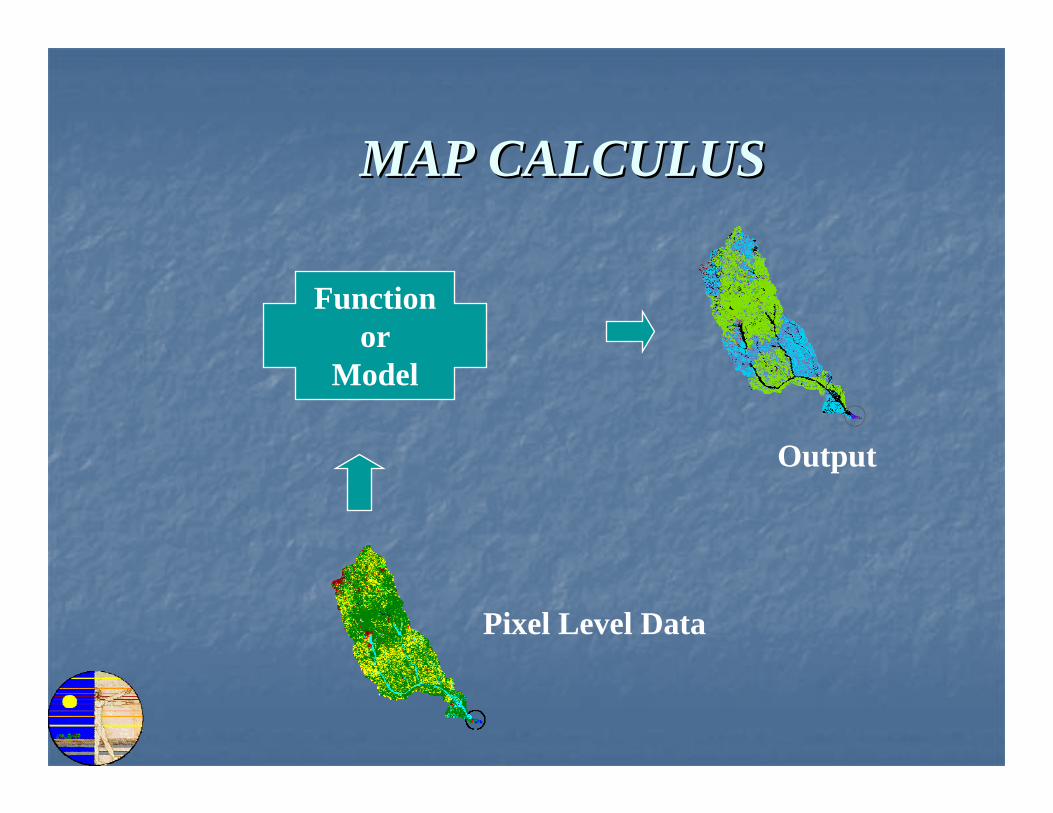
MAP CALCULUSMAP CALCULUS

Pixel Level Data

Output

Functionor

Model

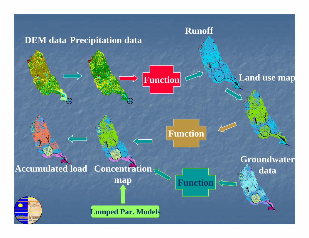
DEM data Precipitation data

Land use map

Concentrationmap

Accumulated load

Function

Function

Function

Groundwaterdata

Lumped Par. Models

Runoff

WHAT IS A SCALE?WHAT IS A SCALE?

Spatial or temporal dimensions at Spatial or temporal dimensions at which entities, patterns, and which entities, patterns, and processes can be observed and processes can be observed and characterized to capture the characterized to capture the important details of a important details of a hydrologic/hydrologic/hydrogeologichydrogeologic process.process.

SCALINGSCALING

The transfer of data or information The transfer of data or information across scales or linking subacross scales or linking sub--process process models through a unified scale is models through a unified scale is referred to as referred to as ““scaling.scaling.””

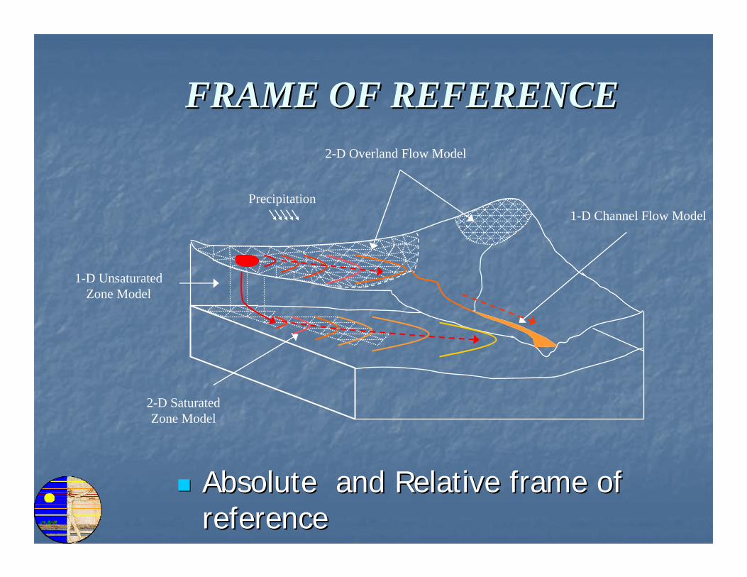
FRAME OF REFERENCEFRAME OF REFERENCE

Absolute and Relative frame of Absolute and Relative frame of referencereference

Precipitation

2-D Overland Flow Model

1-D Channel Flow Model

2-D SaturatedZone Model

1-D UnsaturatedZone Model

SCALE EFFECTSSCALE EFFECTS

Heterogeneity.Heterogeneity.

SubSub--process scales.process scales.

Nonlinearity.Nonlinearity.

SCALING PROBLEMSSCALING PROBLEMS

When largeWhen large--scale models are used to scale models are used to predict smallpredict small--scale events, or when smallscale events, or when small--scale models are used to predict largescale models are used to predict large--scale events, problems may arise.scale events, problems may arise.

Problems also arise when integrated Problems also arise when integrated models are used across scales.models are used across scales.

FUNCTIONAL SCALEFUNCTIONAL SCALE

At what spatial and temporal scale At what spatial and temporal scale does the final model performs does the final model performs optimally; and,optimally; and,

What scale should be selected to What scale should be selected to implement the final integrated implement the final integrated model? model?

SUBSUB--PROCESSESPROCESSES

Integrated river channel flow and groundwater flow.

Integrated overland flow, unsaturated and saturated groundwater flow.

Integrated watershed model.

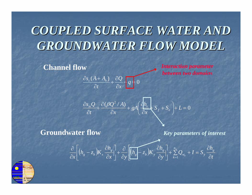
COUPLED SURFACE WATER AND COUPLED SURFACE WATER AND GROUNDWATER FLOW MODELGROUNDWATER FLOW MODEL

0)(=−

∂∂

+∂+∂ q

xQ

tAAs oc

0)/( 2

=+⎟⎠⎞

⎜⎝⎛ ++∂∂

+∂

∂+

∂∂ LSS

xhgA

xAQ

tQs

efrm β

( ) ( )t

hSIQ

yh

Kzhyx

hKzh

xg

y

n

kw

gybg

gxbg

w

k ∂

∂=+∑+⎥

⎦

⎤⎢⎣

⎡∂

∂−

∂∂

+⎥⎦

⎤⎢⎣

⎡∂

∂−

∂∂

=1

Channel flow

Groundwater flow

Interaction parameterbetween two domains

Key parameters of interest

zbDatum

hg

hr

mr

zr

AQUIFER

Impervious Layer

RIVER

wr

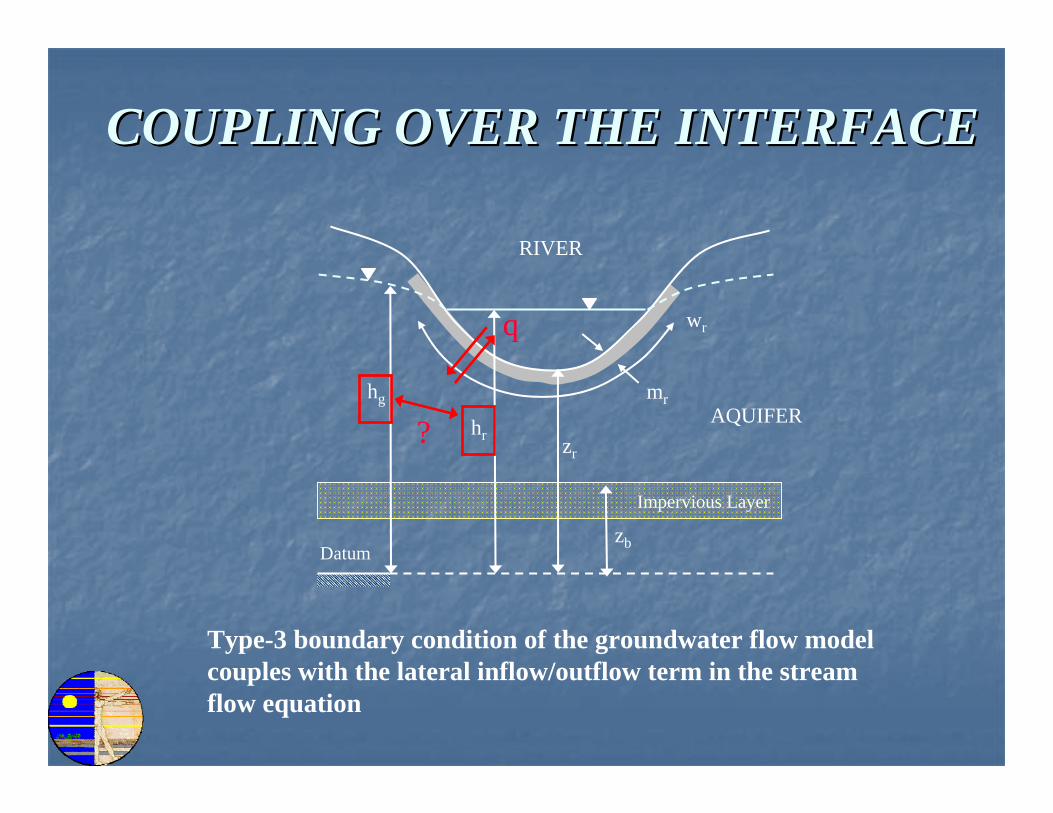
COUPLING OVER THE INTERFACECOUPLING OVER THE INTERFACE

Type-3 boundary condition of the groundwater flow model couples with the lateral inflow/outflow term in the stream flow equation

q

?

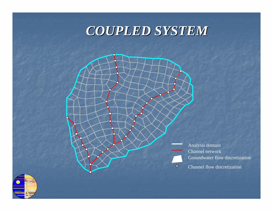
Analysis domain

Groundwater flow discretizationChannel network

Channel flow discretization

COUPLED SYSTEMCOUPLED SYSTEM

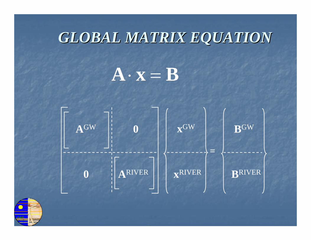
0

0AGW

=

BGW

BRIVER

xGW

xRIVERARIVER

GLOBAL MATRIX EQUATIONGLOBAL MATRIX EQUATION

BxA =⋅

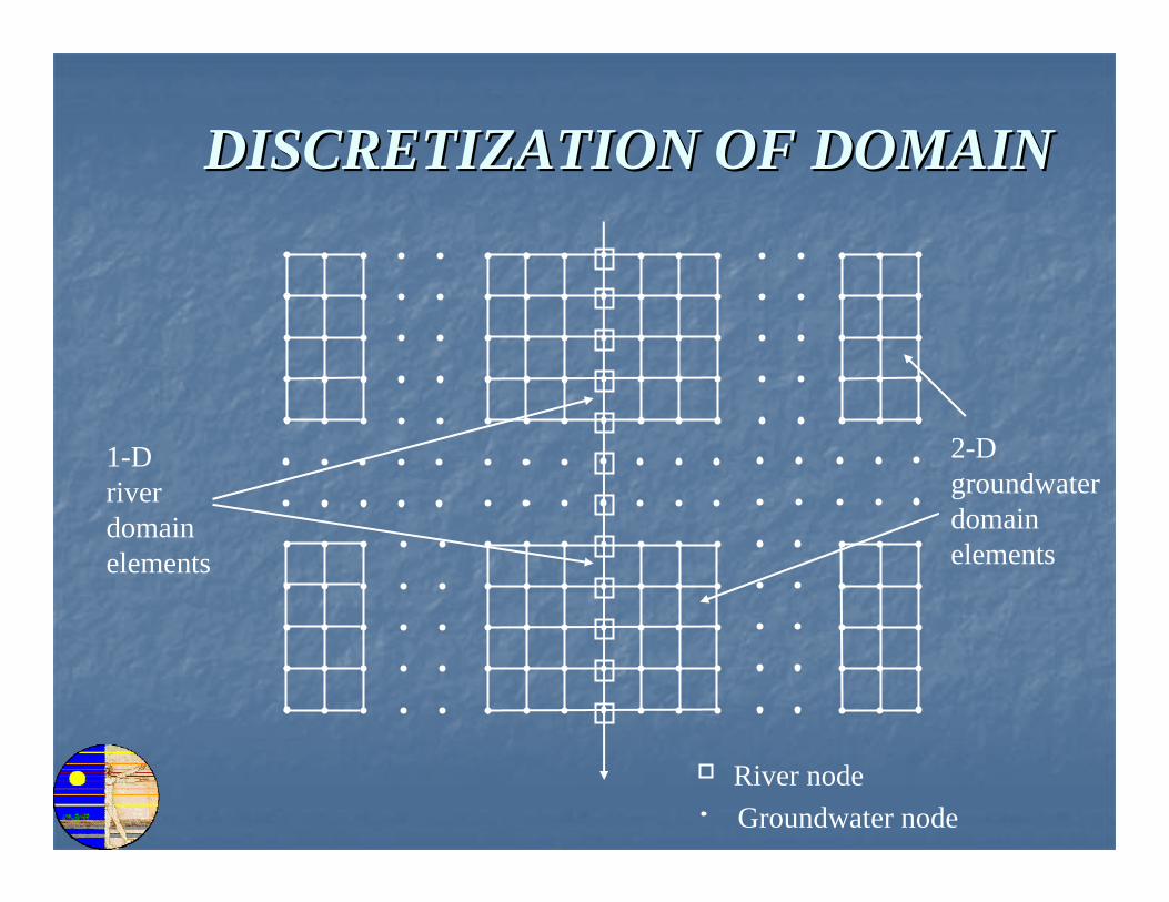
2-Dgroundwaterdomain elements

1-Driver domain elements

River nodeGroundwater node

DISCRETIZATION OF DOMAINDISCRETIZATION OF DOMAIN

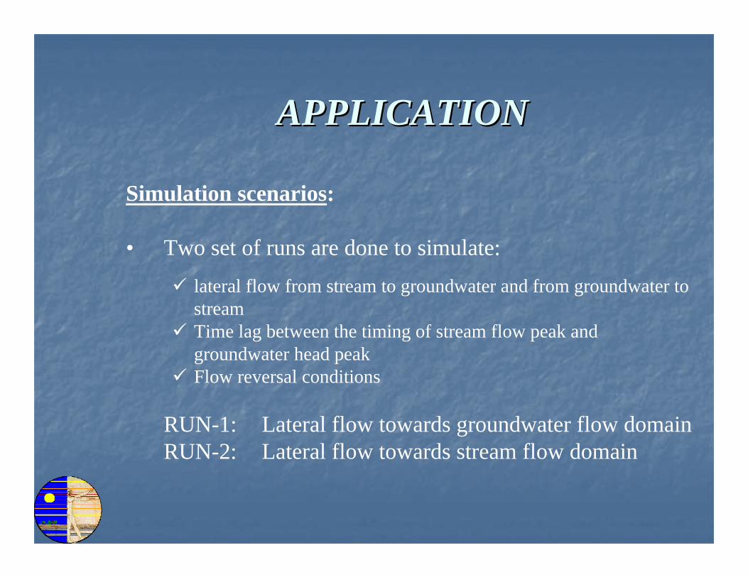
APPLICATIONAPPLICATION

Simulation scenarios:

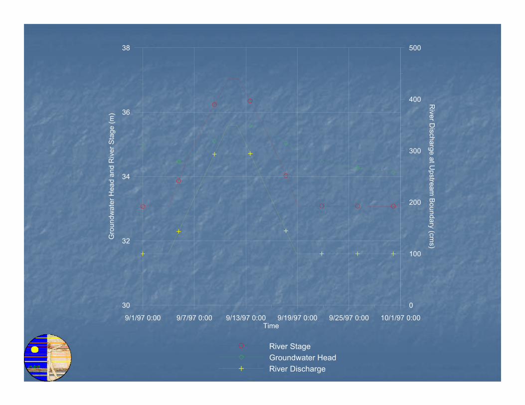
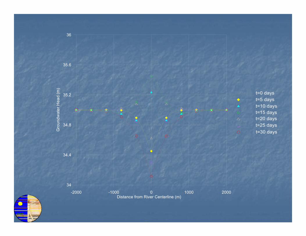
• Two set of runs are done to simulate:lateral flow from stream to groundwater and from groundwater to streamTime lag between the timing of stream flow peak and groundwater head peakFlow reversal conditions

RUN-1: Lateral flow towards groundwater flow domainRUN-2: Lateral flow towards stream flow domain

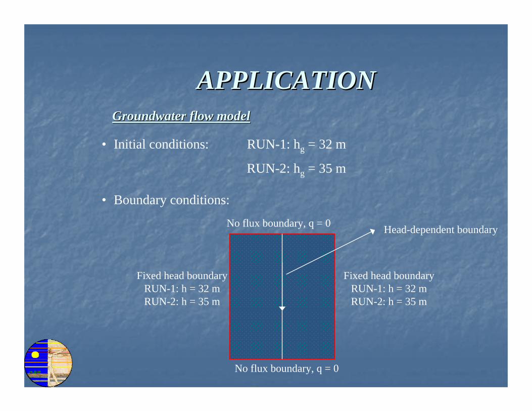
Groundwater flow modelGroundwater flow model

• Initial conditions: RUN-1: hg = 32 m

RUN-2: hg = 35 m

APPLICATIONAPPLICATION

• Boundary conditions:

No flux boundary, q = 0

No flux boundary, q = 0

Fixed head boundaryRUN-1: h = 32 mRUN-2: h = 35 m

Fixed head boundaryRUN-1: h = 32 mRUN-2: h = 35 m

Head-dependent boundary

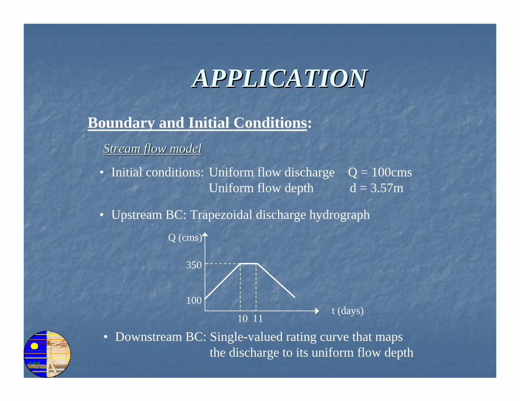
APPLICATIONAPPLICATIONBoundary and Initial Conditions:

Stream flow modelStream flow model

• Upstream BC: Trapezoidal discharge hydrograph

• Initial conditions: Uniform flow discharge Q = 100cms Uniform flow depth d = 3.57m

• Downstream BC: Single-valued rating curve that maps the discharge to its uniform flow depth

t (days)

Q (cms)

10

100

350

11

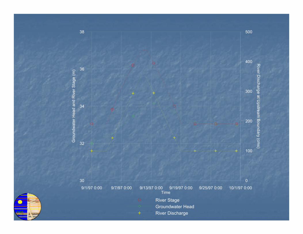
River DischargeGroundwater HeadRiver Stage

9/1/97 0:00 9/7/97 0:00 9/13/97 0:00 9/19/97 0:00 9/25/97 0:00 10/1/97 0:00Time

30

32

34

36

38

Gro

undw

ater

Hea

d an

d R

iver

Sta

ge (m

)

0

100

200

300

400

500

River D

ischarge atUpstream

Boundary

(cms)

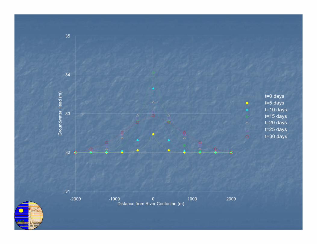
-2000 -1000 0 1000 2000Distance from River Centerline (m)

31

32

33

34

35

Gro

undw

ater

Hea

d (m

)

t=0 dayst=5 dayst=10 dayst=15 dayst=20 dayst=25 dayst=30 days

River DischargeGroundwater HeadRiver Stage

9/1/97 0:00 9/7/97 0:00 9/13/97 0:00 9/19/97 0:00 9/25/97 0:00 10/1/97 0:00Time

30

32

34

36

38

Gro

undw

ater

Hea

d an

d R

iver

Sta

ge (m

)

0

100

200

300

400

500

River D

ischarge atUpstream

Boundary

(cms)

-2000 -1000 0 1000 2000Distance from River Centerline (m)

34

34.4

34.8

35.2

35.6

36

Gro

undw

ater

Hea

d (m

)

t=0 dayst=5 dayst=10 dayst=15 dayst=20 dayst=25 dayst=30 days

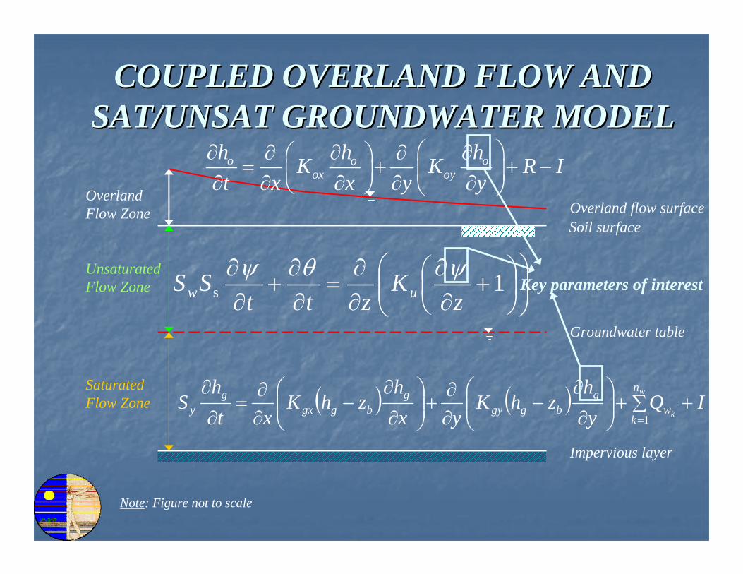
Soil surface

Groundwater table

SaturatedFlow Zone

UnsaturatedFlow Zone

OverlandFlow Zone Overland flow surface

Impervious layer

Note: Figure not to scale

Key parameters of interest

o o oox oy

h h hK K R It x x y y

⎛ ⎞∂ ∂ ∂∂ ∂⎛ ⎞= + + −⎜ ⎟⎜ ⎟∂ ∂ ∂ ∂ ∂⎝ ⎠ ⎝ ⎠

( ) ( ) IQyh

zhKyx

hzhK

xth

Sw

k

n

kw

gbggy

gbggx

gy +∑+⎟⎟

⎠

⎞⎜⎜⎝

⎛∂

∂−

∂∂

+⎟⎟⎠

⎞⎜⎜⎝

⎛∂

∂−

∂∂

=∂

∂=1

⎟⎟⎠

⎞⎜⎜⎝

⎛⎟⎠⎞

⎜⎝⎛ +∂∂

∂∂

=∂∂

+∂∂ 1s z

Kztt

SS uwψθψ

COUPLED OVERLAND FLOW AND COUPLED OVERLAND FLOW AND SAT/UNSAT GROUNDWATER MODELSAT/UNSAT GROUNDWATER MODEL

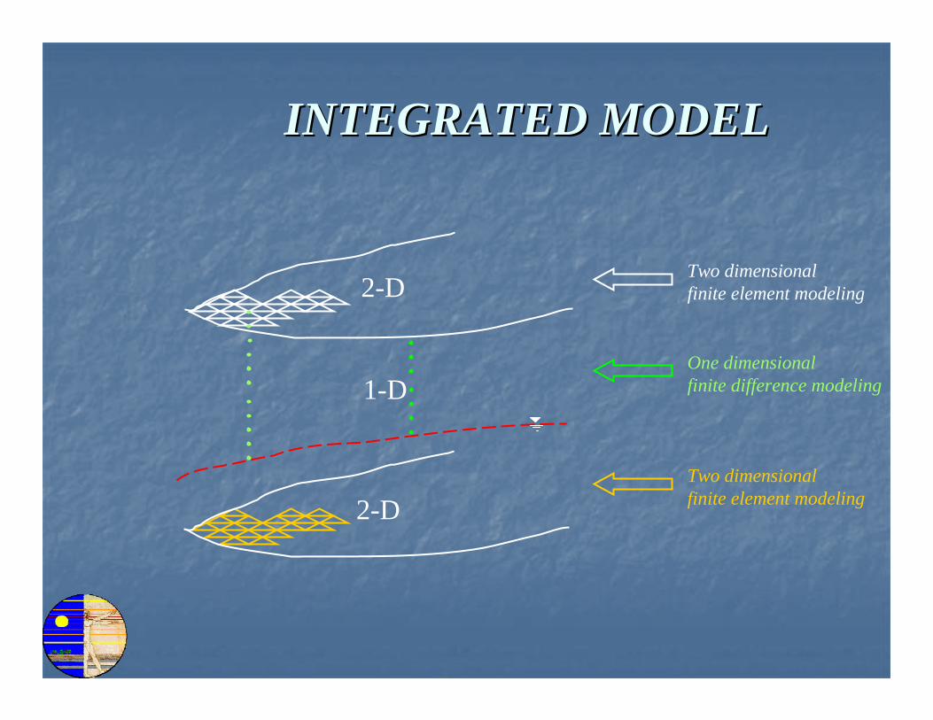
2-D

2-D

1-D

INTEGRATED MODELINTEGRATED MODEL

Two dimensional finite element modeling

One dimensional finite difference modeling

Two dimensional finite element modeling

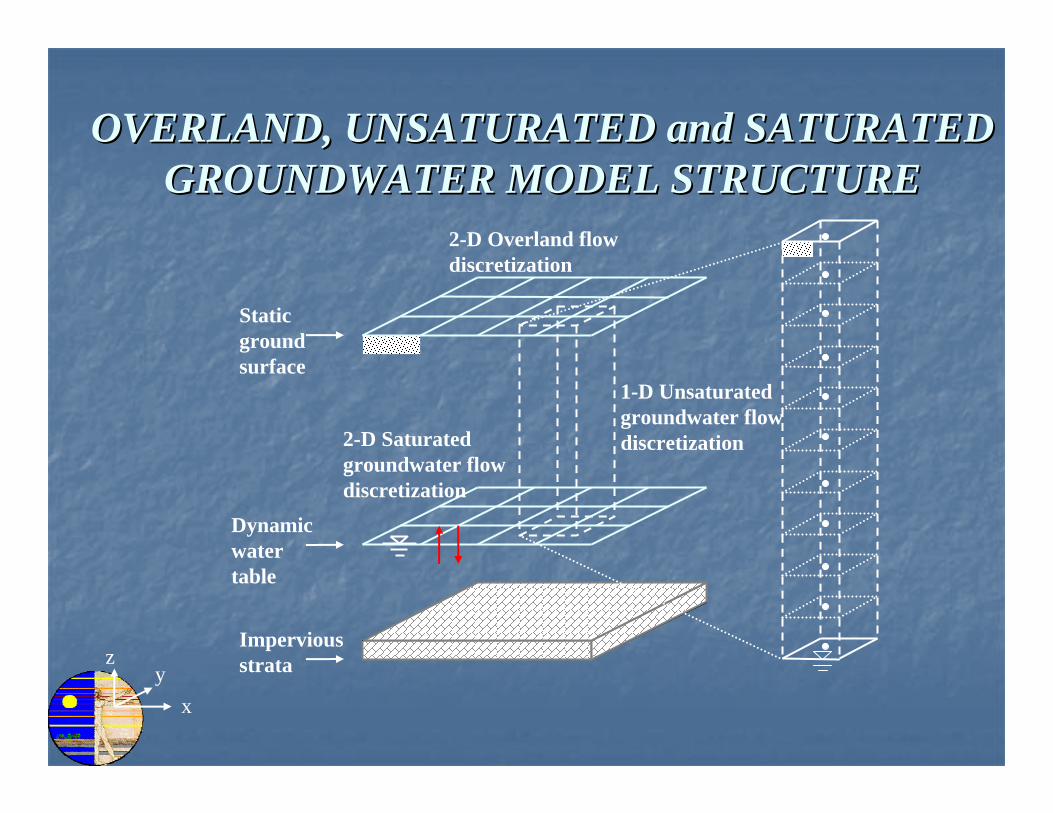
Dynamicwater table

Staticground surface

Imperviousstrataz

yx

2-D Overland flowdiscretization

2-D Saturatedgroundwater flowdiscretization

1-D Unsaturatedgroundwater flow discretization

OVERLAND, UNSATURATED and SATURATED OVERLAND, UNSATURATED and SATURATED GROUNDWATER MODEL STRUCTUREGROUNDWATER MODEL STRUCTURE

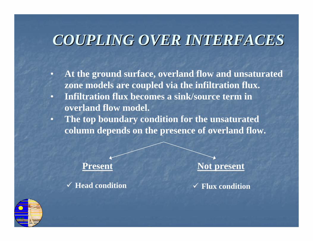
COUPLING OVER INTERFACESCOUPLING OVER INTERFACES

• At the ground surface, overland flow and unsaturated zone models are coupled via the infiltration flux.

• Infiltration flux becomes a sink/source term in overland flow model.

• The top boundary condition for the unsaturated column depends on the presence of overland flow.

Present Not present

Head condition Flux condition

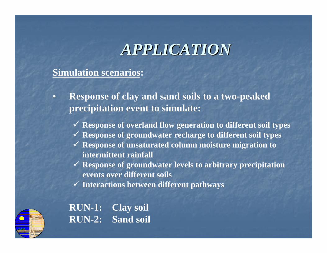
APPLICATIONAPPLICATIONSimulation scenarios:

• Response of clay and sand soils to a two-peaked precipitation event to simulate:

Response of overland flow generation to different soil typesResponse of groundwater recharge to different soil typesResponse of unsaturated column moisture migration to intermittent rainfallResponse of groundwater levels to arbitrary precipitation events over different soilsInteractions between different pathways

RUN-1: Clay soilRUN-2: Sand soil

APPLICATIONAPPLICATIONPhysical Setup:

• 40 m wide X 500 m long hypothetical rectangular plot0 < x < 500 m and 0 < y < 40 m

• Uniform slope in x-direction, Sox = 0.001 m/m• No slope in y-direction, Soy = 0.0 m/m• Essentially one-dimensional flow• Response to a two-peaked precipitation event:

0 2000 4000 6000Time (sec)

0

2E-005

4E-005

6E-005

8E-005

0.0001

Rai

nfal

l Rat

e (m

/s)

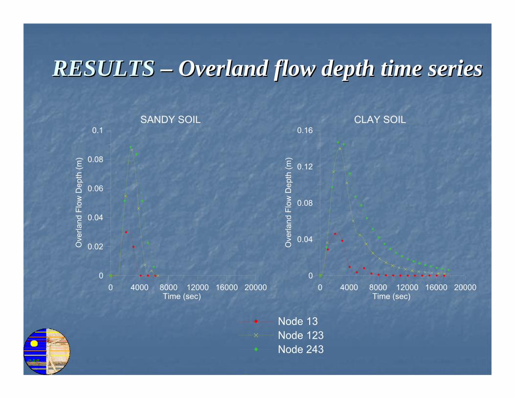
RESULTSRESULTS –– Overland flow depth time seriesOverland flow depth time series

0 4000 8000 12000 16000 20000Time (sec)

0

0.04

0.08

0.12

0.16

Ove

rland

Flo

w D

epth

(m)

CLAY SOIL

Node 13Node 123Node 243

0 4000 8000 12000 16000 20000Time (sec)

0

0.02

0.04

0.06

0.08

0.1

Ove

rland

Flo

w D

epth

(m)

SANDY SOIL

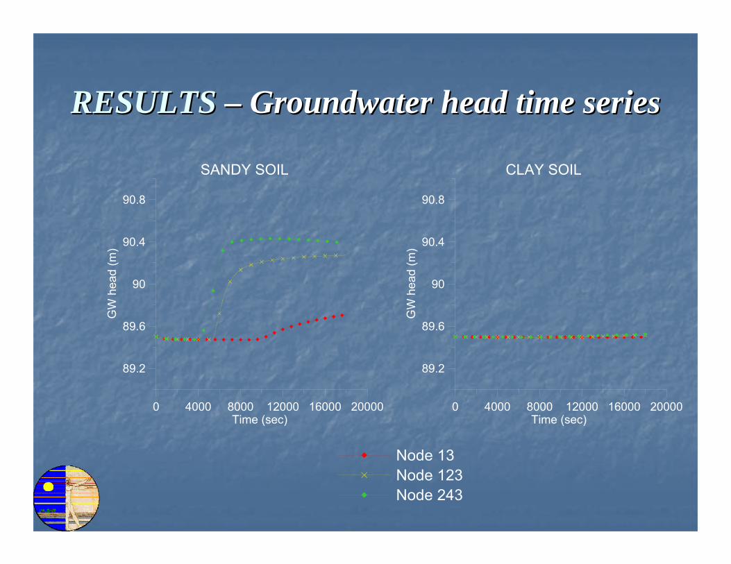
RESULTS RESULTS –– Groundwater head time seriesGroundwater head time series

0 4000 8000 12000 16000 20000Time (sec)

89.2

89.6

90

90.4

90.8

GW

hea

d (m

)

SANDY SOIL

Node 13Node 123Node 243

0 4000 8000 12000 16000 20000Time (sec)

89.2

89.6

90

90.4

90.8

GW

hea

d (m

)

CLAY SOIL

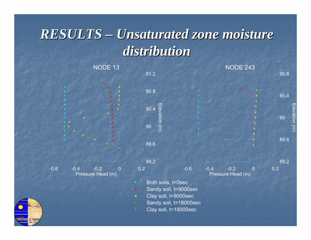
RESULTSRESULTS –– Unsaturated zone moisture Unsaturated zone moisture distributiondistribution

-0.6 -0.4 -0.2 0 0.2Pressure Head (m)

89.2

89.6

90

90.4

90.8

Elevation

(m)

NODE 243

Both soils, t=0secSandy soil, t=9000sec Clay soil, t=9000secSandy soil, t=18000secClay soil, t=18000sec

-0.6 -0.4 -0.2 0 0.2Pressure Head (m)

89.2

89.6

90

90.4

90.8

91.2

Elevation

(m)

NODE 13

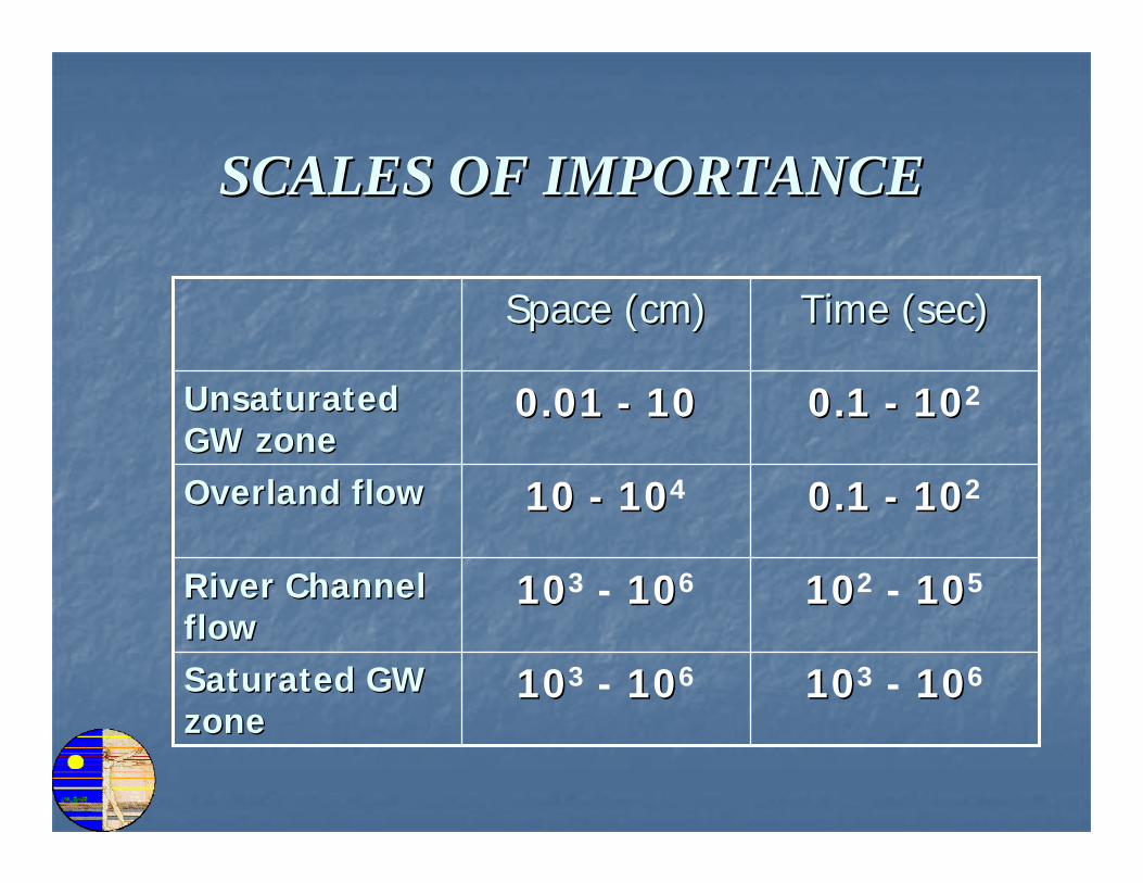
SCALES OF IMPORTANCESCALES OF IMPORTANCE

10103 - 1010610103 - 10106Saturated GW Saturated GW zonezone

10102 - 1010510103 - 10106River Channel River Channel flowflow

0.1 0.1 -- 1010210 10 -- 10104Overland flowOverland flow

0.1 0.1 -- 101020.01 0.01 -- 1010Unsaturated Unsaturated GW zoneGW zone

Time (sec)Time (sec)Space (cm)Space (cm)

HYBRID MODELS ARE THEHYBRID MODELS ARE THE

SOLUTION TO INTEGRATEDSOLUTION TO INTEGRATED

WATERSHED MODELING WATERSHED MODELING SYSTEMSSYSTEMS

APPLICATION:APPLICATION:

Analysis of Coastal Georgia EcosystemStressors Using GIS Integrated RemotelySensed Imagery and Modeling:A Pilot Study for Lower Altamaha River Basin

http://groups.ce.gatech.edu/Research/MESL/research/altamaha/index.htm

Georgia Sea Grant College Program of the National Sea Grant Program.

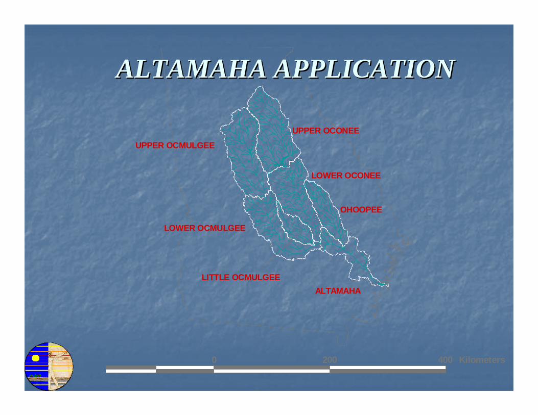
LOWER OCMULGEE

UPPER OCMULGEEUPPER OCONEE

OHOOPEE

ALTAMAHA

LOWER OCONEE

LITTLE OCMULGEE

0 200 400 Kilometers

ALTAMAHA APPLICATIONALTAMAHA APPLICATION

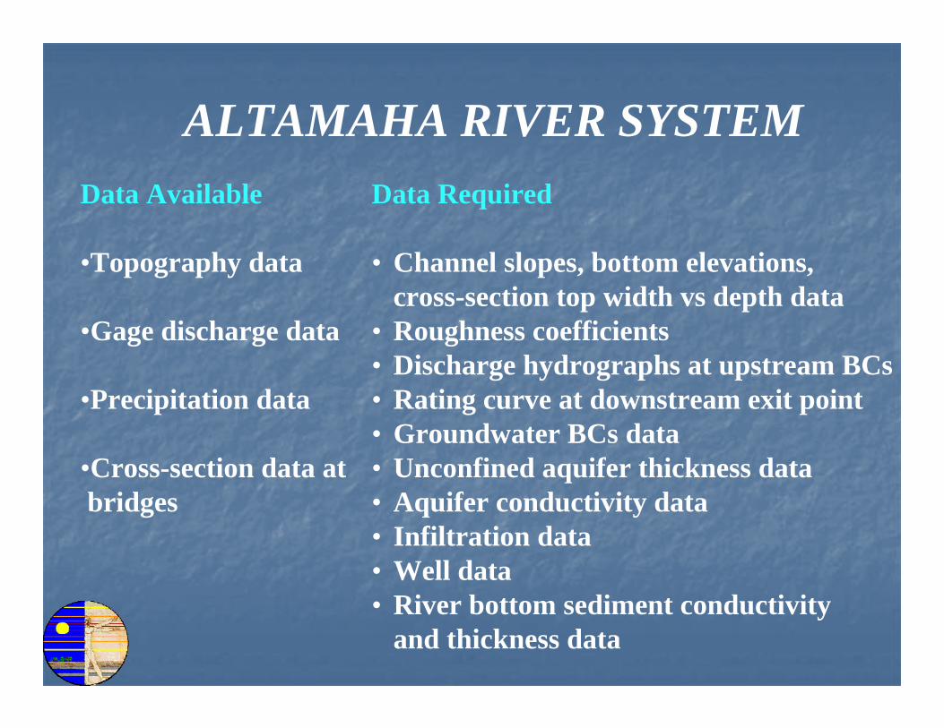
ALTAMAHA RIVER SYSTEMData Required

• Channel slopes, bottom elevations,cross-section top width vs depth data

• Roughness coefficients• Discharge hydrographs at upstream BCs• Rating curve at downstream exit point• Groundwater BCs data• Unconfined aquifer thickness data• Aquifer conductivity data• Infiltration data• Well data• River bottom sediment conductivity

and thickness data

Data Available

•Topography data

•Gage discharge data

•Precipitation data

•Cross-section data at bridges

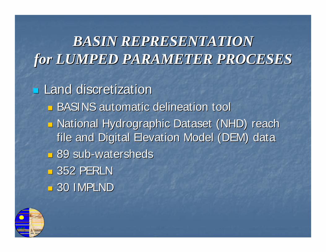
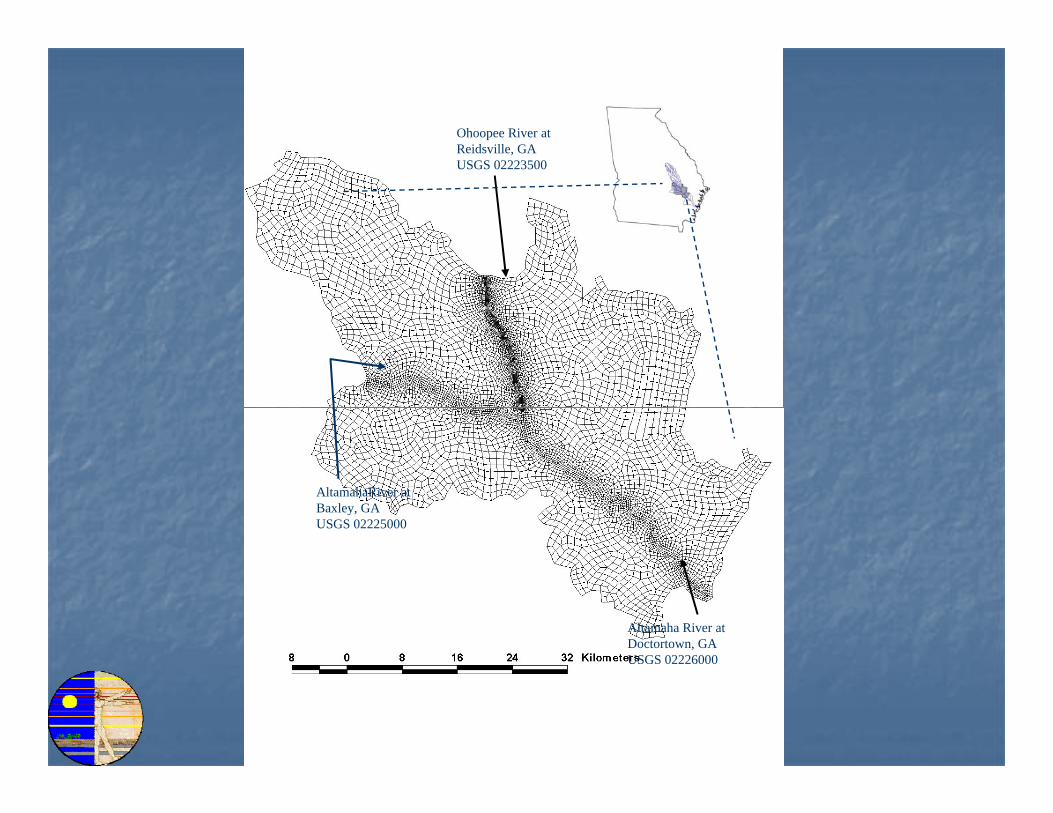
BASIN REPRESENTATIONBASIN REPRESENTATIONfor LUMPED PARAMETER PROCESESfor LUMPED PARAMETER PROCESES

Land discretizationLand discretizationBASINS automatic delineation toolBASINS automatic delineation toolNational Hydrographic Dataset (NHD) reach National Hydrographic Dataset (NHD) reach file and Digital Elevation Model (DEM) data file and Digital Elevation Model (DEM) data 89 sub89 sub--watershedswatersheds352 PERLN352 PERLN30 IMPLND30 IMPLND

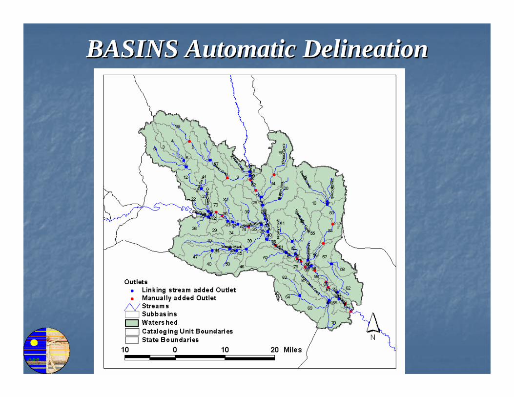
BASINS Automatic DelineationBASINS Automatic Delineation

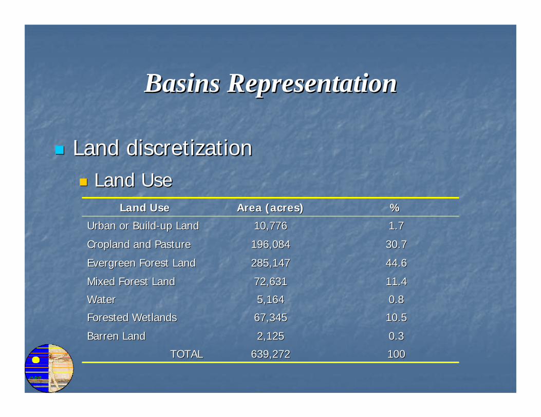
Basins RepresentationBasins Representation

Land discretizationLand discretizationLand UseLand Use

11.411.472,63172,631Mixed Forest LandMixed Forest Land

0.30.32,1252,125Barren LandBarren Land

%%Area (acres)Area (acres)Land UseLand Use

1.71.710,77610,776Urban or BuildUrban or Build--up Land up Land

30.730.7196,084196,084Cropland and Pasture Cropland and Pasture

44.644.6285,147285,147Evergreen Forest LandEvergreen Forest Land

100100639,272639,272TOTALTOTAL

10.510.567,34567,345Forested WetlandsForested Wetlands

0.80.85,1645,164WaterWater

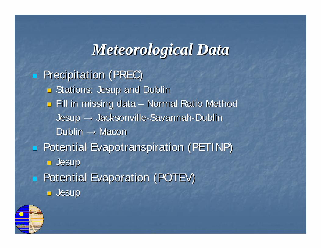
Meteorological DataMeteorological DataPrecipitation (PREC)Precipitation (PREC)

Stations: Stations: JesupJesup and Dublinand DublinFill in missing data Fill in missing data –– Normal Ratio Method Normal Ratio Method JesupJesup →→ JacksonvilleJacksonville--SavannahSavannah--DublinDublinDublin Dublin →→ MaconMacon

Potential Potential EvapotranspirationEvapotranspiration (PETINP)(PETINP)JesupJesup

Potential Evaporation (POTEV)Potential Evaporation (POTEV)JesupJesup

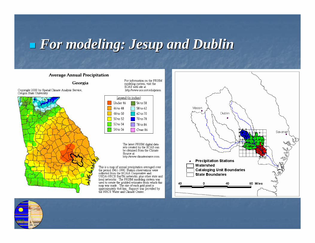
For modeling: For modeling: JesupJesup and Dublinand Dublin

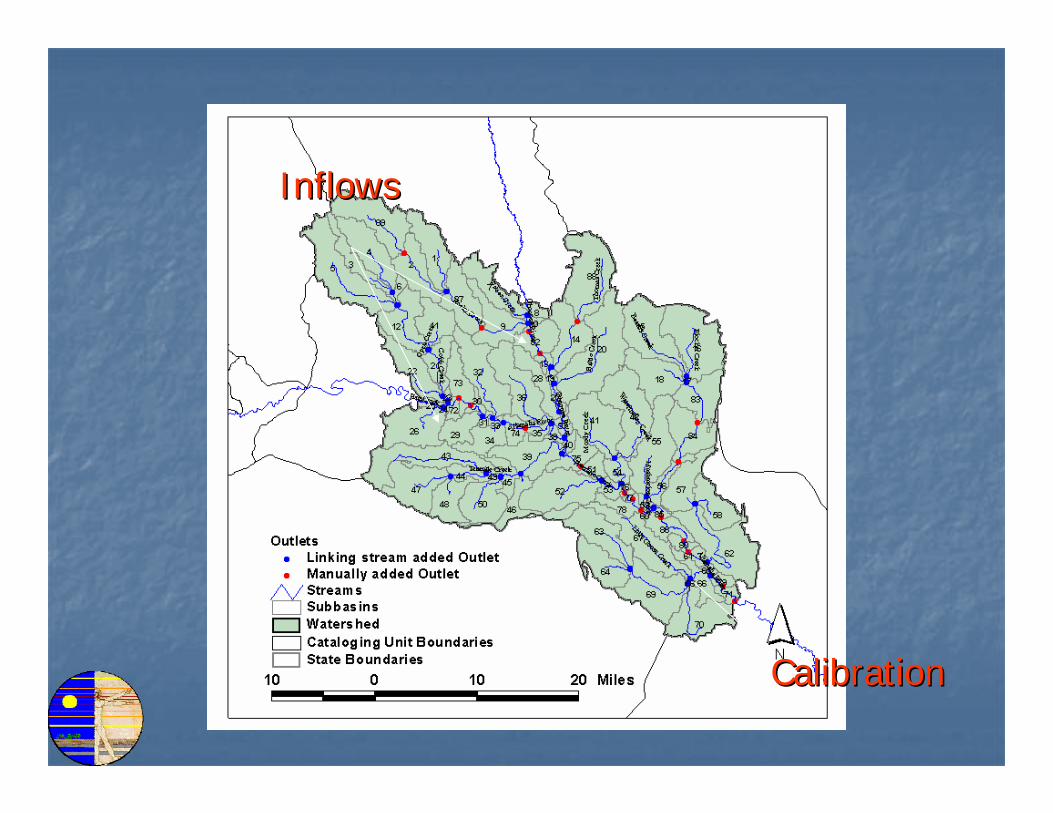
InflowsInflows

CalibrationCalibration

AltamahaRiver

OhoopeeRiver

USGS 02225000Baxley, GA

USGS 02225500Reidsville, GA

USGS 02226000Doctortown, GA

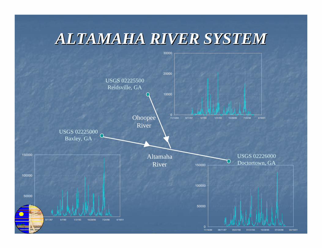
ALTAMAHA RIVER SYSTEMALTAMAHA RIVER SYSTEM

0

50000

100000

150000

11/14/84 8/11/87 5/7/90 1/31/93 10/28/95 7/24/98 4/19/01

0

10000

20000

30000

11/14/84 8/11/87 5/7/90 1/31/93 10/28/95 7/24/98 4/19/01

0

50000

100000

150000

11/14/84 08/11/87 05/07/90 01/31/93 10/28/95 07/24/98 04/19/01

Ohoopee River at Reidsville, GAUSGS 02223500

AltamahaRiver at Baxley, GAUSGS 02225000

Altamaha River at Doctortown, GAUSGS 02226000

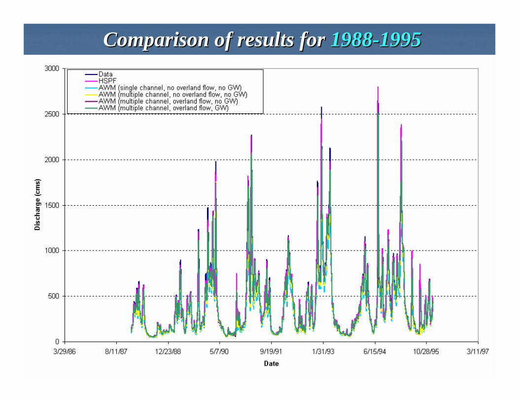
Comparison of results for Comparison of results for 19881988--19951995

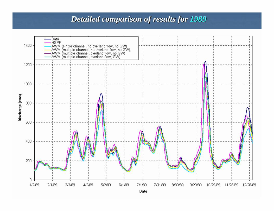
Detailed comparison of results for Detailed comparison of results for 19891989

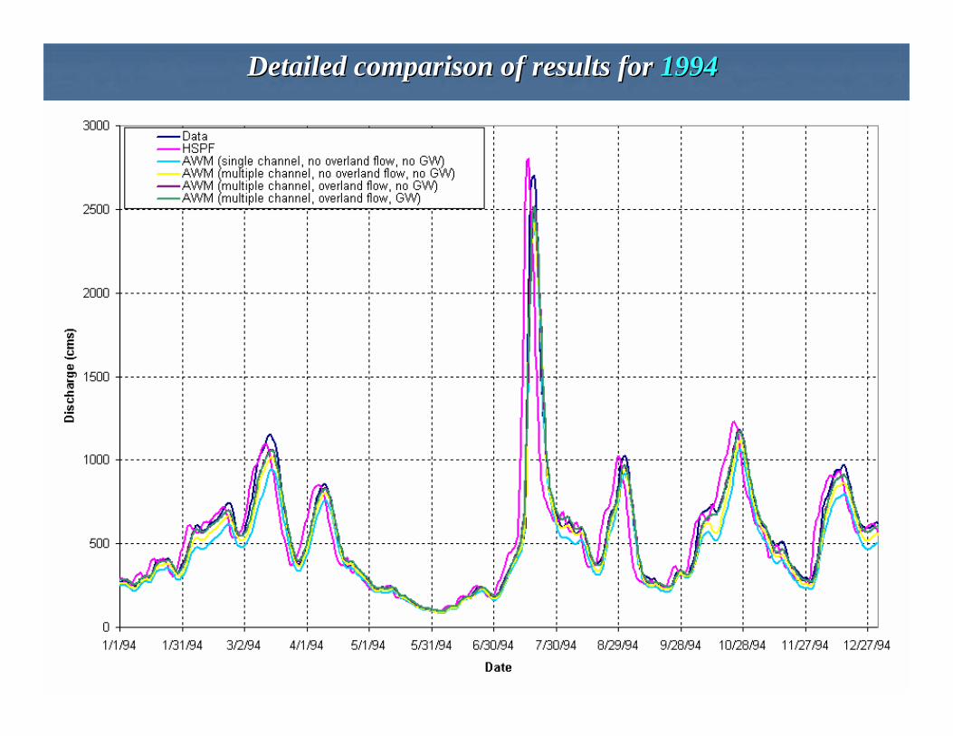
Detailed comparison of results for Detailed comparison of results for 19941994

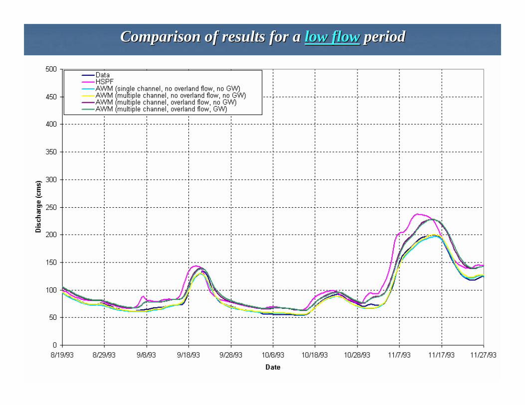
Comparison of results for a Comparison of results for a low flowlow flow period period

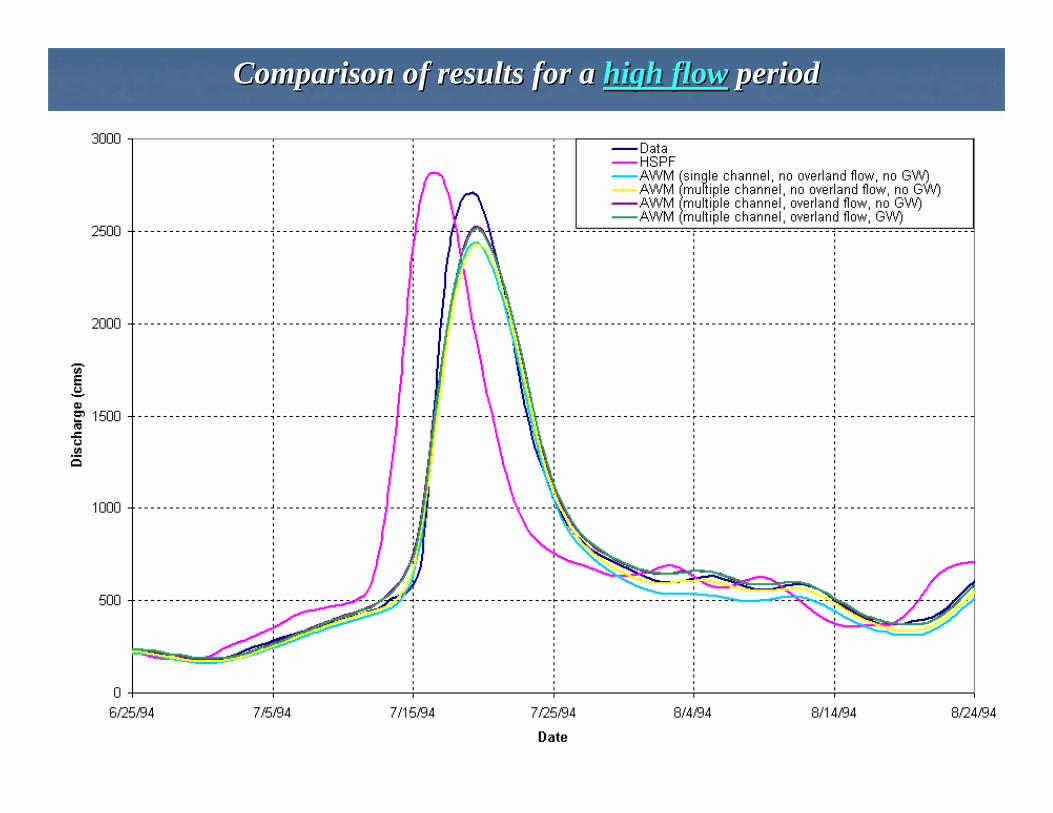
Comparison of results for a Comparison of results for a high flowhigh flow period period

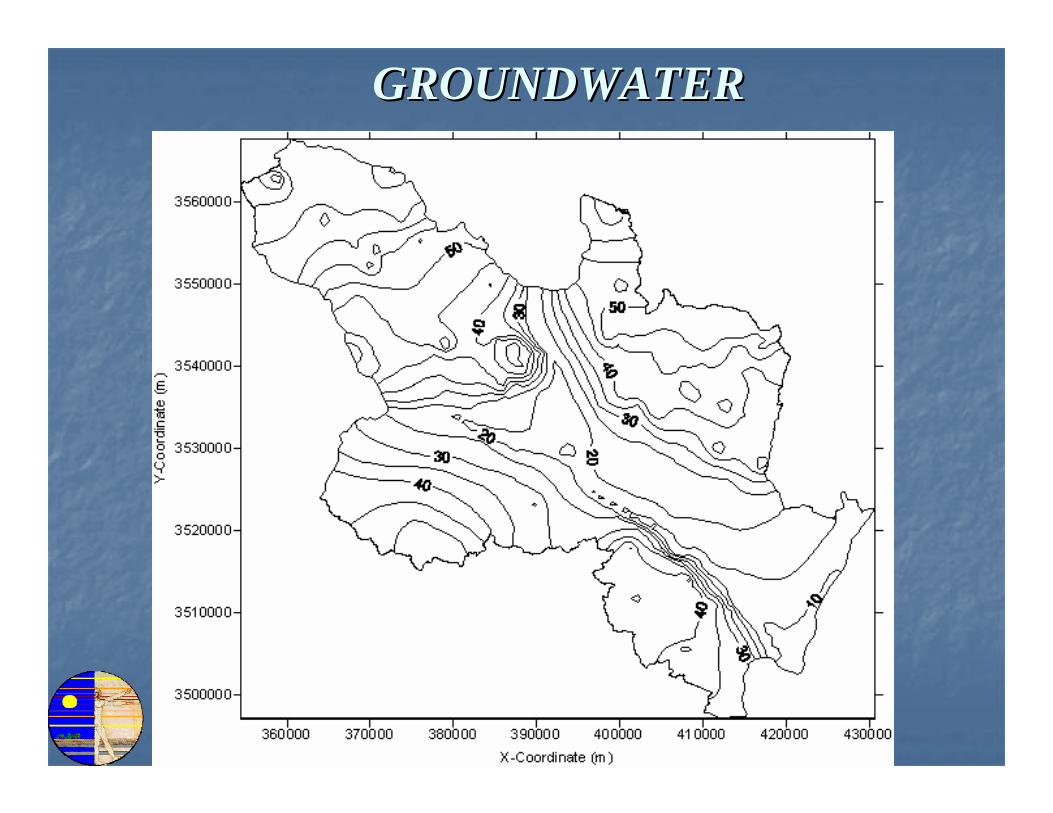
GROUNDWATERGROUNDWATER

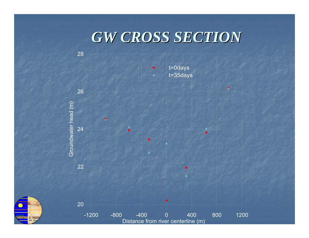
GW CROSS SECTIONGW CROSS SECTION

-1200 -800 -400 0 400 800 1200Distance from river centerline (m)

20

22

24

26

28

Gro

undw

ater

hea

d (m

)t=0dayst=35days

CONCLUSIONSCONCLUSIONS

Order of importance of the subOrder of importance of the sub--process;process;

Domain of importance;Domain of importance;

Functional scales; and,Functional scales; and,

Hybrid modeling concepts Hybrid modeling concepts

CONCLUSIONSCONCLUSIONS

Selection of the smallest scale in an Selection of the smallest scale in an integrated model as functional scale is not integrated model as functional scale is not possible.possible.

Hybrid modeling approach is necessary.Hybrid modeling approach is necessary.

Functional scale based on .....Functional scale based on .....

ACKNOWLEDGEMENTS

This research is partly sponsored by the Georgia Sea Grant College Program.

We would like to express our gratitude to Dr. Mac RawsonDr. Mac Rawson, Director of Georgia Sea Grant College Program for his continuous support throughout this study.

For additional information or For additional information or questions, you may contact:questions, you may contact:

M. M. Aral: maral@ce.gatech.eduhttp://groups.ce.gatech.edu/Research/MESL/

MESLMESLMESL