ORIGINAL PAPER Open Access

Saving and investment causality: implicationsfor financial integration in transition countriesof Eastern Europe

Manuchehr Irandoust1

# The Author(s) 2017. This article is an open access publication

Abstract Numerous studies have been devoted to the Feldstein-Horioka puzzle.However, no consensus has been reached in the literature. This paper examinesthe causal relationship between domestic saving and investment rates in sixtransition economies (Estonia, Latvia, Lithuania, Ukraine, Belarus, and RussianFederation). Theoretically, the presence of any type of causal structure betweenthese two series in a country implies that national capital markets are not open;hence capital flows are impeded. Therefore, the paper employs the bootstrappanel Granger causality approach that accounts for both cross-sectional depen-dence and slope heterogeneity across countries to determine the causal struc-ture. The findings show that there is a causality between the series, therebyimplying that capital is not perfectly mobile internationally in any of thecountries under review, but it is more mobile in Estonia, Russian Federation,and Latvia than Lithuania, Belarus, and Ukraine. The underdevelopment offinancial markets in these countries as well as the demand for foreign capitalto finance domestic investment projects and the lack of adequate economic andfinancial reforms might have driven these results.

Keywords Capital mobility . Saving . Investment . Eastern Europe . Causality

JEL classification F3 . F4

Int Econ Econ PolicyDOI 10.1007/s10368-017-0390-6

* Manuchehr Irandoustmanuchehr.irandoust@hkr.se; manuch.dost@gmail.com

1 School of Business Studies, Department of Economics and Finance, Kristianstad University, 29139 Kristianstad, Sweden

1 Introduction

This paper examines the causal linkage between saving and investment for sixEastern European countries (Estonia, Latvia, Lithuania, Ukraine, Belarus, andRussian Federation). In their seminal work, Feldstein and Horioka (1980)examined the relationship between saving and investment, and they foundsaving and investment to be highly positively correlated in 16 OECD countriesand suggested that international capital mobility was low in these countries.Therefore, if the capital markets are integrated, domestic investment could befinanced by foreign savings, and domestic saving could also seek out higherforeign return, thereby implying a low correlation between saving and invest-ment. In the presence of integration of current financial markets, this resultreveals a contradiction, which is currently known as the Feldstein-Horiokapuzzle. Many theoretical and empirical studies have attempted to resolve thispuzzle in the past three decades.

On the one hand, previous studies have confirmed the Feldstein and Horiokafindings using a variety of approaches and employing cross-sectional, time-series and panel data. On the other hand, several papers have challengedFeldstein and Horioka’s conclusion. Theoretically, in the short-run a positivesaving-investment correlation may arise, despite capital being perfectly mobileacross national borders, because of country-size (Harberger 1980; Murphy 1984;Baxter and Crucini 1993; Bahmani-Oskooee and Chakrabarti 2005), common-ness in technological or productivity shocks (Rasin 1993; Glick and Rogoff1995; Eiriksson 2011), non-traded goods (Frankel 1986; Dooley et al. 1987),current account targeting (Summers 1982), endogenous fiscal policy (Levy1995), international trading costs (Backus et al. 1992; Obstfeld and Rogoff2000), long-run solvency constraint (Coakley et al. 1996), financial frictions(Bai and Zhang 2010), common deflator (Chu 2012) and long-run risk compo-nent in the shock process (Chang and Smith 2014).

Nonetheless, most previous studies are subject to criticism. The cross-sectionstudies in literature on the saving-investment relationship have several limita-tions which are well-known (eg., Sinn 1992). In the case of time-series studies,inferences about the existence of cointegration suffer from well-known powerdeficiencies and it has been argued that the saving-investment associationcaptures some degree of international capital mobility so that it reflects asystemic property because capital mobility in one country must imply mobilityin at least one other country so that the notion of measuring capital mobilitycountry by country is somewhat anomalous (Feldstein and Bachetta 1991).

The panel cointegration approach adopted in many studies also has somedeficiencies which stem from stationarity problems, cross-sectional dependenceand slope homogeneity assumptions. The panel cointegration approach adoptedin this paper circumvent these problems by simultaneously allowing forcountry-specific differences in the form of unobserved country effects unlikecross-country studies and combining information from the time series dimensionwith that obtained from the cross section of units. Furthermore, it has twoimportant advantages. First, it is not required to test the unit root andcointegration (i.e. the variables are used in their levels, without any stationarity

M. Irandoust

conditions). Second, additional panel information can also be obtained given thecontemporaneous correlations across countries (i.e. the equations denote aSeemingly Unrelated Regressions system- SUR system). To the best of theauthor’s knowledge, this paper is the first to apply the bootstrap panel Grangercausality approach to examine the relationship between saving and investment.

The remainder of this paper is organized as follows: Section 2 reviews some stylizedfacts about economic and financial structure of the sample countries. Section 3 providesempirical framework, data, and methodology. Section 4 presents the empirical results.Section 5 offers some discussion. Section 6 concludes.

2 Some stylized facts

2.1 Baltic states1

After regaining independence in 1991, the governments of the Baltics startedcomprehensive programs of economic and political reform. In order to achieveeconomic growth and improve living standards, the Baltics made a rapid shiftfrom a planned economy to an open market system by establishing the relevantlegal framework and economic institutions. The priority was given to theliberalization of prices, external trade, and a stable exchange system, as wellas to the privatization of small and medium-size enterprises. The Baltic coun-tries liberalized their capital accounts relatively quickly compared to othertransition countries. The economic situation in early 1990s was very difficultas real output contracted sharply and prices soared. The economic and politicalcollapse of the Soviet Union created very high inflation that sharply erodedliving standards. The trade and financial links between the independent BalticStates and other countries were disrupted, generating a number of demand andsupply shocks such as major adjustment in the relative prices of tradable goods,loss of traditional export markets in the East, as well as dis-functioning ofpayment and monetary arrangements.

Under these circumstances, the Baltic States found little scope for a gradu-alist approach in policy response. The Baltics introduced their own currencieswith fixed exchange rates relatively early during transition because it wasbelieved that fixed exchange rate arrangements were more suited in light oflack of accumulated experience with independent central banking. Fixed ex-change rate regimes, supported by tight fiscal policies and structural reforms,helped to restore macroeconomic stability and contain inflation in the region.Thereafter, output stabilized relatively rapidly and economic recovery began inEstonia, Latvia, and Lithuania in 1994 and GDP growth turned positive inEstonia, Lithuania, and Latvia. During 1995–1998 average GDP growth rangedfrom 6.6% in Estonia to 4% in Latvia. Despite the liberalization of most prices,inflation was quickly brought under control. CPI inflation dropped from almost1000% in 1992 to below 30% in all three countries by 1996 and declined to a

1 This part is mainly based on European Commission (2009, 2010, 2015), Grigonytė (2010), and UNCTAD(2016).

Saving and investment causality

single digit by 1998. On the other hand, the current account deficit started toincrease rapidly from 1994, and amounted to 5.5% of GDP in Latvia, 10% inLithuania, and 11% in Estonia by 1997.

The privatization-related FDI inflows covered a part of the domestic saving-investment gap, e.g., in 1993–1997 average annual FDI inflows amounted to6% of GDP in Estonia and Latvia, but only 2% in Lithuania. In Estonia, mostsmall enterprises were privatized by heavily on vouchers but also used tendersfor strategic investors. Furthermore, improved bankruptcy procedures and mod-ernized legal and regulatory framework also played an important role inreforming the economies. Estonia was slightly ahead of the other two Balticsin this area. Compared to other transition economies, the Baltics made fasterprogress in reducing the role of the state in the economy and creating abusiness-friendly environment. Tight fiscal policy was a very important factorcontributing to the stabilization and reform process. The level of governmentspending and public debt was lower in the Baltics than in the EU-15 and othertransition economies.

As a result of the prudent fiscal policies in the Baltics the debt remainedvery low by international standards. In 1995, Estonian debt equaled 9% of GDPand declined to 3.5% in 2007. Latvian debt remained rather low until 2007,close to 9% of GDP. In Lithuania, the debt-to-GDP ratio was on an increasingtrend until 2000 but started to decline afterwards mainly due to strong GDPgrowth and in 2007 it was equal to 17% of GDP. The first real economic shockfor the Baltic economies after the collapse of the planned economy took placewith the Russian financial crisis in 1998. The crisis caused a recession in theBaltic states and this was accompanied by a collapse in trade and losses in thefinancial system. On the real side, Baltic exporters, which were dependent onRussian markets, were dealing with a very sharp deterioration in terms of tradefollowing the devaluation of the rouble by more than 70% during 1998–1999,while imported Russian commodities were linked to the U.S. dollar.

Although Russia’s share of the Baltics’ external trade had declined evenbefore the crisis, it remained at around one-fifth of exports for Estonia andLatvia, and around one third in Lithuania. In 1999, economic growth turnednegative in Estonia and Lithuania, and dropped sharply in Latvia. In all threecountries, the budget surpluses also turned into deficits. In parallel with thetrade crisis, the financial sector faced loan losses from their exposures tocompanies which were dependent on the Russian market. The adjustment phase,which started already before the financial turmoil began to unfold in 2008, wasconsiderably intensified by global developments. In 2009, GDP decreased byalmost 13% in Estonia, 18.0% in Latvia and Lithuania. However, GDP growthrates for the three Baltic countries remain at around 3% per year during 2013–2015.

However, FDI inflows to the Baltic countries were attracted by differentfactors during the decade of economic transition. On the one hand, FDI wasmainly driven by the availability of relatively low-cost resources as the privat-ization process created business opportunities for foreign investors in themanufacturing sector. On the other hand, an underdeveloped services sectoropened up scope for horizontal FDI. Particularly, the privatization of public

M. Irandoust

utilities and liberalization of the banking sector attracted significant FDI in-flows. At the same time, the Baltic states’ convenient geographical location,located between the EU, Russia and the Commonwealth of Independent States(CIS) countries, as well as EU membership attracted efficiency-seeking FDI.The successful structural reforms and a relatively stable macroeconomic envi-ronment were the main reasons for attracting FDI to the Baltics.

FDI into Estonia amounted to $2799 million in 2005, $1565 million in 2012,$546 million in 2013, and $208 million in 2015. In Latvia, FDI was $2324million in 2007, $1453 million in 2011, $1109 million in 2012, and $643million in 2015. FDI into Lithuania amounted to $2015 million, $1446 million,$469 million, and $863 million in 2007, 2011, 2013, and 2015, respectively.On average, FDI inflows during the period 1993–2014 were 7.24% of GDP inEstonia, 3.87% in Latvia, and 2.91% in Lithuania. Estonia has outperformed theother two countries since 1997, when it overtook Latvia, and especially sinceEU accession. This was largely due to the establishment of Nordic banks inEstonia. Analyzing the various components of FDI for the three Baltic countriesover the last decades, it shows that FDI inflows in Latvia and Lithuania havebeen dominated by equity capital, (mostly in the form of acquisitions and greenfield investment), while Estonia has received on average a much higher shareof reinvested earnings probably due to the Estonian corporate tax system whichwas reformed in 2000. The tax rate on reinvested earnings was reduced to zero,whereas the tax on corporate income was set to 21% in order to support theaccumulation of domestically-generated capital.

Generally speaking, all Baltic countries have been quite successful withrespect to structural reforms, Estonia has moved not only faster than itsneighbors with the timing and the implementation of reforms but also carriedout more reforms in the areas of enterprise and competition policy than Latviaand Lithuania. The two latter types of reform would reduce the abuse of marketpower and improve effective corporate control exercised through domesticfinancial institutions and markets, thereby supporting market-drivenrestructuring.

2.2 Russian Federation, Belarus, and Ukraine2

Ukraine

Shortly after independence in August 1991, the Ukrainian Government lib-eralized most prices and created a legal framework for privatization, butwidespread resistance to reform within the government and the legislaturehindered reform efforts and led to some backtracking. Consequently, outputby 1999 had fallen to less than 40% of the 1991 level. Sharply decliningoutput, lack of access to financial markets, and massive monetary expansionto finance government spending resulted in hyperinflation. Thus, in 1996 theUkrainian central bank replaced the old currency, the karbovanets, with the

2 This part is mainly based on The Economist (2014), KPMG (2011, 2013), Mehmet Ogutcu (2002), Cooper(2009), and UNCTAD (2016).

Saving and investment causality

hryvnia and attempted to keep it stable in relation to the dollar. The currencycontinued to be unstable through the late 1990s.

Once Russia started to raise energy prices (in the aftermath of gradualadjustment of its own relative price structure), Ukraine was badly hit becauseof the high-energy intensity of Ukraine’s economy (high percentage of themetal industry for instance). This made the Ukrainian economy vulnerable toexternal shocks. The IMF encouraged Ukraine to quicken the pace and scope ofreforms to promote economic growth. Ukrainian Government officials eliminat-ed most tax and customs privileges in 2005 budget law, brought more economicactivity out of Ukraine’s large shadow economy, but more improvements wereneeded, including fighting corruption, developing capital markets, and improv-ing the legislative framework. The economy contracted around 15% in 2009,among the worst economic performances in the world. The government issuedshort-term debt at interest rates as high as 15% and many analysts were worriedthat the country will soon default on its debt.

After the global crisis, and as the euro crisis intensified, Ukraine sufferedfrom a drought in capital flows which put strong downward pressure on thehryvnia. Protecting the currency drained the central bank’s reserves, whichdropped from a high of $40 billion in 2011 to about $12 billion in 2014.Then, the central bank admitted defeat and let the currency float. Currencydepreciation was an economic headache for Ukraine in the short term. Abouthalf of its public debt was in foreign currencies: as the hrvynia lost value,Ukraine’s debt burden rose. Moreover, Ukraine was badly hit by the financialcrisis which resulted in GDP to fall by 15% in 2009. In 2010, the IMF agreedto loan Ukraine $15 billion. The IMF ended up freezing the deal in 2011 afterKiev failed to touch the costly subsidies.

Progressively lowering the rate of corporation tax has also weakened thestate’s finances. Corruption, poor governance, interstate conflict, and politicalsituation are other major problems. The Ukrainian shadow economy is one ofthe biggest in the world-at around 50% of GDP, according to IMF. Businessesoperating underground tend not to pay taxes, further depriving the governmentof funds. Ukraine needed to find about $25 billion in 2014 to finance its largecurrent-account deficit and to meet foreign creditors. FDI was $267 million,$10,913 million, $8401 million, $4499 million, $410 million, and $2961 mil-lion in 1995, 2008, 2012, 2013, 2014, and 2015, respectively. However, thelevel of reforms in Ukraine with respect to privatization, banking reforms, andinfrastructure have been half-hearted.

2.2.1 Russian Federation

The first seven years of Russia’s transition from the Soviet central plannedeconomy (1991–1998) were not easy. During the period, Russia lost 30% of itsGDP and also suffered very high rates of inflation- over 2000% in 1992 andover 800% in 1993- before it declined to more tolerable levels of around 20%by the end of the 1990s. Nevertheless, the country’s fixed exchange rate regimetogether with its fragile fiscal position appeared to be unsustainable when theinternational markets got affected by spillover effects of financial distress

M. Irandoust

elsewhere in the world. In the course of 1998, the outbreak of a severebanking, currency and sovereign debt crisis could not be prevented. This ledto a significant decrease in the value of the ruble, eventually forcing theRussian government to devalue the ruble in 1998. Russia did not performmuch better in the foreign sector and FDI flows were not significant giventhe size and needs of the Russian economy. The cumulative figure for FDI inRussia from 1991 through the end of 2001 shows $18.2 billion, or only 5% ofdomestic fixed capital formation.

Furthermore, Russia was incurring serious capital flight- some $150 billionworth between 1992 and 1999. During the period, the Russian government hadlarge budget deficits that reached as high as 9.8% of GDP, forcing the govern-ment to finance debt at very high interest rates. Russia’s economic problemsintensified by the financial crisis in 1998. The crisis led to the demise of manyRussian banks which had held government debt. The crisis caused: Russianinterest rates soared aimed inconsistent macroeconomic policy which triggeredthe crises. Hence, prices on the Russian stock market plummeted; and the valueof the Russian ruble sank. During 1998, the ruble lost 60% of its (nominal)value in terms of the dollar. In addition, foreign reserves decreased substantiallyduring that time. The reserves, including gold, dropped from $18.4 billion to$12.5 billion, and real GDP declined 4.9% in 1998.

Russian economy was vulnerable because of more fundamental problems related tothe economic policy and economic structure. These included the failure to institute taxreform, property rights, and bankruptcy laws and procedures. Later on, Russia madesome attempts to perform economic reform during this period by moving from thecentrally planned economic system and introducing market prices for most goods andservices. This made the Russian ruble convertible for trade transactions, and theeconomy was opened to foreign trade and investment.

Russia also lifted its restrictions on capital inflows. After 2005, FDI inflowsgrew exponentially, due to investments in newly liberalized sectors. Afterreaching record heights in 2008, the financial crisis led to a collapse in FDI,as the global economy entered into a recession. Since the severe drop in 2009,FDI has recovered partially, reaching USD 30188 million in 2012, USD 53397million in 2013, USD 29152 million in 2014, and USD 9825 million in 2015.Foreign investors remain motivated by the continued strong growth of theconsumer market and affordable labor costs, together with productivity gains.They also continue to be attracted by high returns in energy and other natural-resource related projects. During 2007–2011, the US was a leading investor inRussia with 122 projects, corresponding to 16% of total projects. The secondlargest investor was Germany, with 99 projects in different sectors. In 2011,investments from the Netherlands accounted for 12% of total FDI in Russia.

2.2.2 Belarus

Since early 2000s, the economic situation in Belarus was characterized by adynamic economic growth. The annual growth rate of GDP at constant pricesover five years through 2008 was around 10%. On the one hand, as a state-dominated economy, with only limited relationships with the world financial

Saving and investment causality

markets, has been less affected by the severe effects of the financial crisis. Onthe other hand, a sharp decline in both Russian economic subsidies and foreigntrade with Russia stemming from the global crisis has had a significant impacton the Belarusian economy, albeit with some lag. Consequently, in 2009, GDPgrowth was marginal at 0.2%, while external financing, primarily from the IMF,allowed for keeping the economy stable. The gradual recovery following in2010 resulted in a substantial increase of wages and the already high level offinancing of government programs. As a result, the annual GDP grew by 7.6%in real terms, which was at the cost of a further increase of the current accountdeficit and inflationary pressures.

This crisis stemmed from the fact that the authorities kept the de-facto fixedexchange rate regime for too long (and the exchange rate remained too strong).As the Russian ruble floated much more freely and Russia reduced the afore-mentioned forms of subsidies (and some other) to Belarus the country’s balanceof payments came under pressure. Significant control and influence of the stateon the economy were the main prerequisites of the crisis. The authorities usedgrowth-promoting policies, expansionary credit practices and broadly appliedgenerous financing of various state programs. This was together with a signif-icant boost of wages and an increase in demand for value-added, primarilyimported goods. Thus, the crisis emerged from devaluation expectations in 2011as a result of diminishing foreign exchange reserves of the National Bank.

To tackle the situation, the government devalued the currency to the basketof currencies by more than 50% (56% to USD). However, this was believed tobe a late and inadequate response, as the National Bank’s foreign reserves werenot sufficient to provide effective support to the market demand of the hardcurrency even after the devaluation. To create the country’s foreign exchangereserves, the authorities were actively looking for external funding, which wasmost likely to come from the foreign anti-crisis organizations and massiveprivatization. The results of the crisis generated a significant effect on allsectors of the economy lacking funds in foreign currencies to pay for importedproduction inputs and goods. While the Government reported a growth of GDPby 11.1% in 2011 on an annual basis, CPI for the six months of the year grewby a record 43.8% since June 2010.

Belarus has a substantial and relatively well-developed industrial base due toits history as an Bassembly plant^ in the former Soviet Union (49% of GDP in1990). The contribution of added value of industry in GDP amounted to 26.8%in 2010. In addition, the country has a broad agricultural base and is fully self-sufficient in agricultural production and also provides export opportunities. TheBelarusian economy is dominated by state controlled sectors. Privatization talkshave been re-activated in 2009 and 2010, partly in response to IMF/ WorldBank recommendations, and again in 2011 as an attempt to tackle the crisis.

FDI into the Belarusian economy was relatively moderate through 1990–2006. Due to the Government’s first steps towards liberalizing the economy andthe promotion of investment opportunities, in 2007 the Belarusian economyreceived USD 1.79 billion of net FDI, five times higher than in 2006. In 2008,the country’s economy received USD 2150 million in FDI. FDI into Belarusamounted to USD 1877 million in 2009, USD 1393 million in 2010, USD 4002

M. Irandoust

million in 2011, USD 1429 million in 2012, USD 2230 million in 2013, USD1828 million in 2014, and USD 1584 million in 2015. However, FDI inBelarus averaged 314.50 USD million from 2000 until 2016, reaching an all-time high of 2734.30 USD million in the fourth quarter of 2011. A majorsource of FDI to Belarus in 2010 was Russia (USD 820.4 million or 60.8% ofgross FDI inflow). Significant shares of FDI originated also from Germany,Switzerland, China, and Iran. Equity injections totally USD 111.3 million alsowent into the banking sector.

3 Empirical framework, data, and methodology

Capital mobility is important issue because, in a world with high capitalmobility, national governments can follow expansionary fiscal policies withoutconfronting large-scale crowding out implied by these policies. Furthermore, theexistence of high capital mobility rules out the constraints imposed by domesticcredit markets and money supplies. Thus, monetary policy is rendered muchless effective under this condition. The presence of internationally mobilecapital also means that capital owners do not bear the full burden of corporateincome tax. In a such environment, capital may freely move to a country wherethe return is higher, i.e., taxes are lower.

The saving-investment approach to capital mobility was first presented byFeldstein and Horioka (1980). It is based on the assumption that, in a worldwith perfect capital mobility, a country will indicate very little correlationbetween domestic saving and investment in the long run. If perfect capitalmobility does not exist, then differences among the country’s investment ratesshould correspond to differences in its respective saving rates. Thus, by com-paring the correlations between domestic saving and investment rates in variouscountries, one can determine the degree of capital mobility.

However, our study is based upon the same postulated relationships betweendomestic investment and saving rates; but it is not concerned with assessing thecorrelation between them. Rather, this study attempts to present further evi-dence on capital mobility by exploring the causal relationship between savingand investment rates in six eastern European countries. In a world withimperfect capital mobility, changes in saving must create changes in investmentand vice versa. Thus, the presence of any form of causal relationship betweenthese two series must be interpreted as an indication that national capitalmarkets are not open; capital flows are hindered; hence there is no financialintegration. If, however, no causality is found, one can conclude that theeconomy is open and capital is mobile (Leachman 1990).

The data are downloaded from the World Bank’s World Development Indi-cators. Given the data availability, the annual data (1995–2014) for the follow-ing economies are used: Estonia, Latvia, Lithuania, Ukraine, Belarus, andRussian Federation. These countries were chosen because of the fact that theywere economically and politically very dependent on the former Soviet Unionand it would be interesting to study their capital markets’ progress after theirindependence. The selection of time period is dictated by the availability of

Saving and investment causality

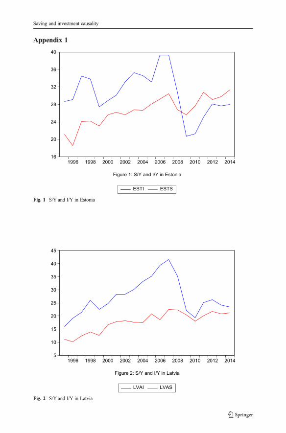
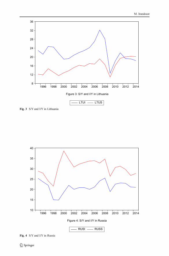
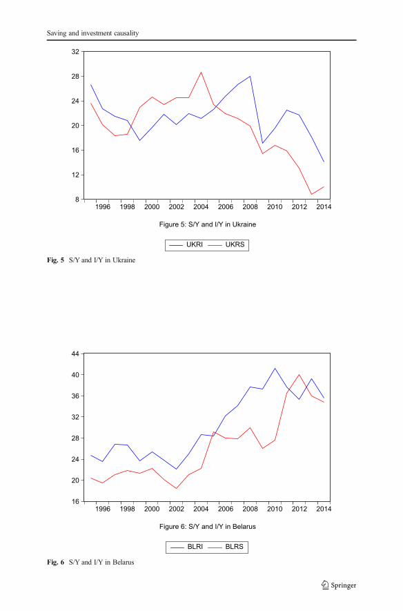
data. Investment (INV) is the ratio of gross domestic investment to GDP (I/Y)and saving (SAV) is the ratio of gross domestic saving to GDP (S/Y). Figures 1,2, 3, 4, 5 and 6 (Appendix 1) illustrates the variables for each country and inAppendix 2, data sources, definition of variables, study period are collectedtogether.

The estimation follows the bootstrap panel Granger causality proposed byKónya (2006). This approach has two important advantages. First, it is notrequired to test the unit root and cointegration (i.e. the variables are used intheir levels, without any stationarity conditions). Second, additional panel in-formation can also be obtained given the contemporaneous correlations acrosscountries (i.e. the equations denote a Seemingly Unrelated Regressions system-SUR system).

Two steps should be followed before applying the bootstrap panel Granger causality:testing the panel for cross-sectional dependence and testing for cross-country hetero-geneity. The first issue implies the transmission of shocks from one variable to others.In other words, all countries in the sample are influenced by globalization and havecommon economic characteristics. The second issue indicates that a significant eco-nomic connection in one country is not necessarily replicated by the others.

A set of three tests is constructed in order to check the cross-sectionaldependence assumption: the Breusch and Pagan (1980) cross-sectional depen-dence (CDBP) test, the Pesaran (2004) cross-sectional dependence (CDP) test,and the Pesaran et al. (2008) bias-adjusted LM test (LMadj). Regarding the country-specific heterogeneity assumption, the slope homogeneity tests ( �Δ andΔ−

adj) of Pesaran

and Yamagata (2008) are used (Appendix 3 provides more information about thesetests). The Kónya's (2006) approach considers both issues, based on SUR systemsestimation and identification of Wald tests with country-specific bootstrap criticalvalues. This procedure allows us to consider all variables in their levels and performcausality output for each country:

SAV1;t ¼ α1;1 þ ∑lm1i¼1β1;1;iSAV1;t−i þ ∑1n1

i¼1δ1;1;iINV1;t−i þ ε1;1;t;SAV2;t ¼ α1;2 þ ∑lm1

i¼1β1;2;iSAV2;t−i þ ∑1n1i¼1δ1;2;iINV2;t−i þ ε1;2;t;

SAVN ;t ¼ α1;N þ ∑lm1i¼1β1;N ;iSAVN ;t−i þ ∑1n1

i¼1δ1;N ;iINVN ;t−i þ ε1;N ;t;

ð1Þ

and

INV1;t ¼ α2;1 þ ∑lm2i¼1β2;1;iSAV1;t−i þ ∑ln2

i¼1δ2;1;iINV1;t−i þ ε2;1;t;INV2;t ¼ α2;2 þ ∑lm2

i¼1β2;2;iSAV2;t−i þ ∑ln2i¼1δ2;2;iINV2;t−i þ ε2;2;t;

INVN ;t ¼ α2;N þ ∑lm2i¼1β2;N ;iSAVN ;t−i þ ∑ln2

i¼1δ2;N ;iINVN ;t−i þ ε2;N ;t;

ð2Þ

In equation systems (1) and (2), SAV is the ratio of gross domestic saving to GDP,INV denotes the ratio of gross domestic investment to GDP, N is the number of panelmembers, t is the time period (t = 1,…,T), and i is the lag length selected in the system.The common coefficient is α, the slopes are β, and δ, while ε is the error term.

M. Irandoust

To test for Granger causality in this system, alternative causal relations for eachcountry are likely to be found: (i) there is one-way Granger causality from X to Y if notall δ1,i are zero, but all β2,i are zero; (ii) there is one-way Granger causality from Y to Xif all δ1,i are zero, but not all β2,i are zero; (iii) there is two-way Granger causalitybetween X and Y if neither δ1,I nor β2,i are zero; and (iv) there is no Granger causalitybetween X and Y if all δ1,i and β2,i are zero. It is also allowed the maximal lags to differacross variables, but the same across equations. In this study, the system is estimated byeach possible pair of lm1, ln1, lm2, and ln2, and it is assumed that 1 to 4 lags exist. Thenthe combinations that minimize the Schwarz Bayesian Criterion are chosen.

By inspecting the data, we find that most break dates correspond tomajor events suchas the financial crisis of 1997–1998 and 2007–2008 and the economic downturn of2001. Due to the existence of these structural breaks, we should incorporate these breaksinto our testing model; otherwise, the results will be biased. Since Kónya (2006) cannotallow different break dates into the testing model, we follow the procedure adopted byTsong and Lee (2011) and Bahmani-Oskooee et al. (2014) to adjust the data as follows:

yt¼ yt−α− ∑

mþ1

l¼1θlDUl;t− ∑

mþ1

i¼1ρiDTi;t−εt; ð3Þ

where, ŷt (either SAVor INV) is adjusted by the effect of possible structural breaks, ytis SAV or INV, DUt and DTt are defined as the following:

DUk;t ¼ 10

�if TBk−1≺t≺TBk

otherwiseð4Þ

DTk;t ¼ t−TBk−10

�i f TBk−1≺t≺TBk

otherwiseð5Þ

4 Estimation results

Table 1 reports the results of cross-sectional dependence tests (CDBP, CDp, and LMadj)and slope homogeneity tests ( �Δ and Δ−

adj). The first set of tests, for cross-sectional

dependence, clearly reveals that the null hypothesis of no cross-sectional dependence isrejected for all significance levels. More precisely, this implies that there is a cross-sectional dependence in the case of our sample countries. Any shock in one country istransmitted to others, the SUR system estimator being more appropriate than country-by-country pooled OLS estimator. The second part of the Table shows that the nullhypothesis of slope homogeneity is rejected for both tests and for all significance levels.In this case, the economic relationship in one country is not replicated by the others. As

Saving and investment causality

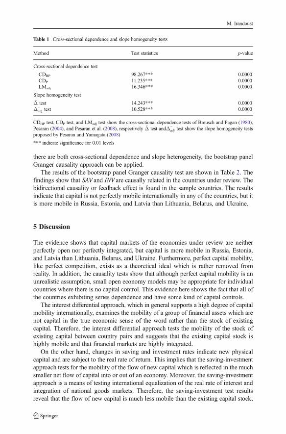
there are both cross-sectional dependence and slope heterogeneity, the bootstrap panelGranger causality approach can be applied.

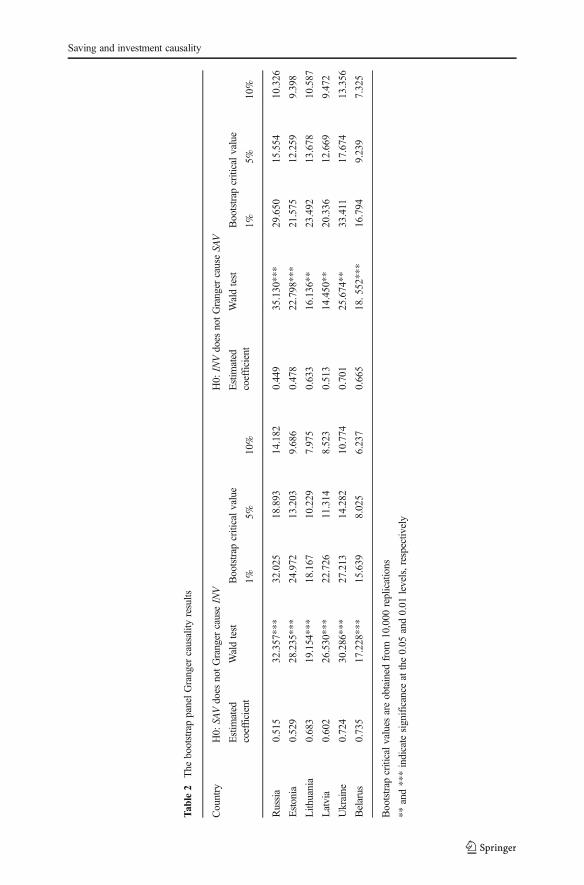
The results of the bootstrap panel Granger causality test are shown in Table 2. Thefindings show that SAV and INV are causally related in the countries under review. Thebidirectional causality or feedback effect is found in the sample countries. The resultsindicate that capital is not perfectly mobile internationally in any of the countries, but itis more mobile in Russia, Estonia, and Latvia than Lithuania, Belarus, and Ukraine.

5 Discussion

The evidence shows that capital markets of the economies under review are neitherperfectly open nor perfectly integrated, but capital is more mobile in Russia, Estonia,and Latvia than Lithuania, Belarus, and Ukraine. Furthermore, perfect capital mobility,like perfect competition, exists as a theoretical ideal which is rather removed fromreality. In addition, the causality tests show that although perfect capital mobility is anunrealistic assumption, small open economy models may be appropriate for individualcountries where there is no capital control. This evidence here shows the fact that all ofthe countries exhibiting series dependence and have some kind of capital controls.

The interest differential approach, which in general supports a high degree of capitalmobility internationally, examines the mobility of a group of financial assets which arenot capital in the true economic sense of the word rather than the stock of existingcapital. Therefore, the interest differential approach tests the mobility of the stock ofexisting capital between country pairs and suggests that the existing capital stock ishighly mobile and that financial markets are highly integrated.

On the other hand, changes in saving and investment rates indicate new physicalcapital and are subject to the real rate of return. This implies that the saving-investmentapproach tests for the mobility of the flow of new capital which is reflected in the muchsmaller net flow of capital into or out of an economy. Moreover, the saving-investmentapproach is a means of testing international equalization of the real rate of interest andintegration of national goods markets. Therefore, the saving-investment test resultsreveal that the flow of new capital is much less mobile than the existing capital stock;

Table 1 Cross-sectional dependence and slope homogeneity tests

Method Test statistics p-value

Cross-sectional dependence test

CDBP

CDP

LMadj

98.267***11.235***16.346***

0.00000.00000.0000

Slope homogeneity test�Δ testΔ−

adj test14.243***10.528***

0.00000.0000

CDBP test, CDP test, and LMadj test show the cross-sectional dependence tests of Breusch and Pagan (1980),Pesaran (2004), and Pesaran et al. (2008), respectively �Δ test andΔ−

adj test show the slope homogeneity testsproposed by Pesaran and Yamagata (2008)

*** indicate significance for 0.01 levels

M. Irandoust

Tab

le2

The

bootstrappanelGranger

causality

results

Country

H0:

SAVdoes

notGranger

causeINV

H0:

INVdoes

notGranger

causeSA

V

Estim

ated

coefficient

Waldtest

Bootstrap

criticalvalue

Estim

ated

coefficient

Waldtest

Bootstrap

criticalvalue

1%5%

10%

1%5%

10%

Russia

0.515

32.357***

32.025

18.893

14.182

0.449

35.130***

29.650

15.554

10.326

Estonia

0.529

28.235***

24.972

13.203

9.686

0.478

22.798***

21.575

12.259

9.398

Lithuania

0.683

19.154***

18.167

10.229

7.975

0.633

16.136**

23.492

13.678

10.587

Latvia

0.602

26.530***

22.726

11.314

8.523

0.513

14.450**

20.336

12.669

9.472

Ukraine

0.724

30.286***

27.213

14.282

10.774

0.701

25.674**

33.411

17.674

13.356

Belarus

0.735

17.228***

15.639

8.025

6.237

0.665

18.5

52***

16.794

9.239

7.325

Bootstrap

criticalvalues

areobtained

from

10,000

replications

**and***indicatesignificance

atthe0.05

and0.01

levels,respectively

Saving and investment causality

and as a by-product, real rates of return are not equal nor are good’s markets integratedacross countries.

According to the analysis of saving and investments causality, the eastern Europeancountries under review are not perfectly integrated into the world capital market.However, they could significantly increase the degree of international capital mobilityby the removal of capital controls and further barriers that limit the import and export ofcapital. In order to avoid the side effects of lifting barriers to capital account activitysuch as crises, an increase in debt, and financial instability, removal of barriers shouldbe coordinated with certain macroeconomic policies. These are: a developed financialsector capable of coping with volatility in capital flows; the steady absence of asubstantial capital account deficit; a sufficient level of international reserve assets; afloating exchange rate; and a cautious fiscal policy.

Beside, a low degree of financial integration as a s result of a high value of savingsretention, it has also been argued that the finding of a high value of savings retentioncoefficients also indicates: (i) high political and currency risk of overseas securities holding;(ii) a low degree of human capital mobility; (iii) a solvency constraint by open capitalmarkets; (iv) a lack of consumption smoothing in response to productivity shocks; and (v)effective use of policy instruments by governments in targeting the current account.3

6 Conclusion

Previous studies of causality and panel cointegration between saving and investmentdoes not consider cross-sectional dependence and slop heterogeneity across countries.On the basis of the bootstrap panel Granger causality test (that accounts for both cross-sectional dependence and heterogeneity across countries), one can conclude that for thecountries under review (Russian Federation, Estonia, Latvia, Lithuania, Belarus, andUkraine) in general, changes in the saving rate lead to changes in the investment rate orvice versa. The underdevelopment of financial markets in these countries as well as thedemand for foreign capital to finance domestic investment projects and the lack ofadequate economic and financial reforms might have driven these results.

The integration of financial markets into the world capital market is important foreconomic growth in eastern European countries since the access to foreign capitalincreases the number of investments and entails the transfer of technology through FDI.Financial market integration is furthermore necessary for an efficient monetary policyin an enlarged monetary union, since different degrees of financial market integrationcause different reactions on monetary shocks.

Acknowledgements The useful comments of three anonymous referees are really appreciated. Of course,any remaining error is mine.

3 These issues have also been discussed in Bahmani-Oskooee and Chakrabarti (2005), Nell and Santos (2008),and Pelgrin and Schich (2008).

M. Irandoust

16

20

24

28

32

36

40

1996 1998 2000 2002 2004 2006 2008 2010 2012 2014

ESTI ESTS

Figure 1: S/Y and I/Y in Estonia

Fig. 1 S/Y and I/Y in Estonia

5

10

15

20

25

30

35

40

45

1996 1998 2000 2002 2004 2006 2008 2010 2012 2014

LVAI LVAS

Figure 2: S/Y and I/Y in Latvia

Fig. 2 S/Y and I/Y in Latvia

Appendix 1

Saving and investment causality

10

15

20

25

30

35

40

1996 1998 2000 2002 2004 2006 2008 2010 2012 2014

RUSI RUSS

Figure 4: S/Y and I/Y in Russia

Fig. 4 S/Y and I/Y in Russia

8

12

16

20

24

28

32

36

1996 1998 2000 2002 2004 2006 2008 2010 2012 2014

LTUI LTUS

Figure 3: S/Y and I/Y in Lithuania

Fig. 3 S/Y and I/Y in Lithuania

M. Irandoust

16

20

24

28

32

36

40

44

1996 1998 2000 2002 2004 2006 2008 2010 2012 2014

BLRI BLRS

Figure 6: S/Y and I/Y in Belarus

Fig. 6 S/Y and I/Y in Belarus

8

12

16

20

24

28

32

1996 1998 2000 2002 2004 2006 2008 2010 2012 2014

UKRI UKRS

Figure 5: S/Y and I/Y in Ukraine

Fig. 5 S/Y and I/Y in Ukraine

Saving and investment causality

Appendix 2

Sample. The annual data (1995–2014) for the following economies are used: Estonia,Latvia, Lithuania, Ukraine, Belarus, and Russian Federation.

Definition of variables. Investment (INV) is the ratio of gross domestic investmentto GDP (I/Y) and saving (SAV) is the ratio of gross domestic saving to GDP (S/Y).

Source of data. The data are downloaded from the World Bank’s World DevelopmentIndicators.

Appendix 3

Cross-sectional dependence testsBreusch and Pagan's (1980) LM test has been used in many empirical

studies to test cross-sectional dependency. LM statistics can be calculated usingthe following panel model:

yit ¼ αi þ β∘

i xit þ μit; i ¼ 1; 2;…;N t ¼ 1; 2;…; T ; ð6Þ

where i is the cross-section dimension, t is the time dimension, xit is k × 1 vector ofexplanatory variables while αi and βi are the individual intercepts and slope coefficientsthat are allowed to differ across states. In the LM test, the null hypothesis of no cross-sectional dependenceH0: Cov(μit,μjt) = 0 for all t and i ≠ j is tested against the alternativehypothesis of cross-sectional dependence H1: Cov(μit,μjt) ≠ 0 for at least one pair of i ≠ j.For testing the null hypothesis, Breusch and Pagan (1980) developed the following test:

CDBP ¼ T ∑N−1

i¼1∑N

j¼iþ1ρ∧2

ij; ð7Þ

where ρ∧2

ijis the estimated correlation coefficient among the residuals obtained from

individual OLS estimation of Eq. (6). Under the null hypothesis, the LM statistic has anasymptotic chi-square distribution with N(N-1)/2 degrees of freedom. Pesaran (2004)proposes that the LM test is only valid when N is relatively small and T is sufficientlylarge. To overcoming this problem, Pesaran (2004) introduces the following LMstatistic for the cross-section dependency test:

CDp ¼ffiffiffiffiffiffiffiffiffiffiffiffiffiffiffiffiffi

1

N N−1ð Þ

s∑N−1

i¼1∑N

j¼iþ1T ρ

∧2

ij−1

!; ð8Þ

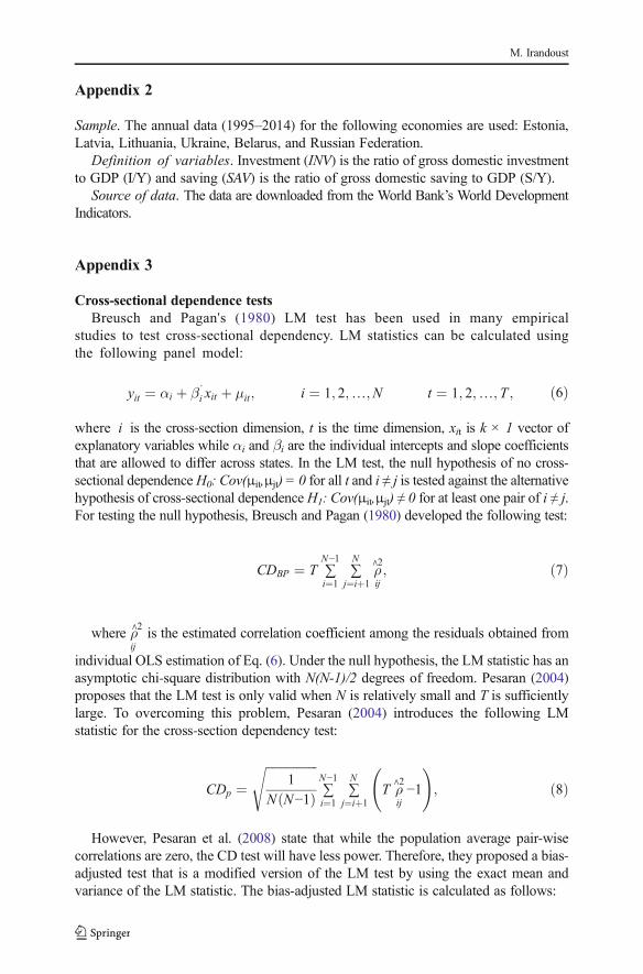
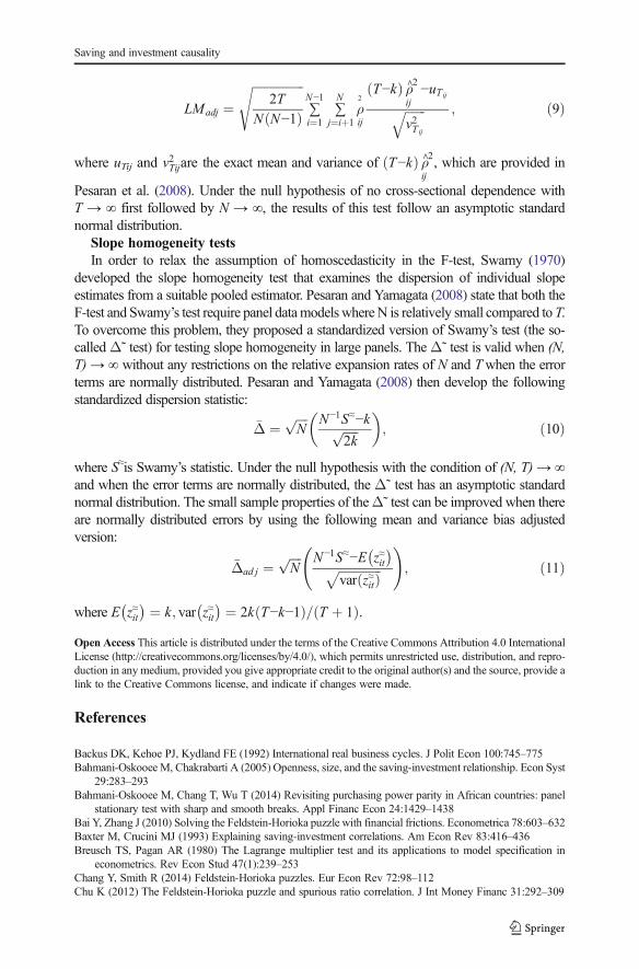
However, Pesaran et al. (2008) state that while the population average pair-wisecorrelations are zero, the CD test will have less power. Therefore, they proposed a bias-adjusted test that is a modified version of the LM test by using the exact mean andvariance of the LM statistic. The bias-adjusted LM statistic is calculated as follows:

M. Irandoust

LMadj ¼ffiffiffiffiffiffiffiffiffiffiffiffiffiffiffiffiffi

2TN N−1ð Þ

s∑N−1

i¼1∑N

j¼iþ1ρ2

ij

T−kð Þ ρ∧2ij

−uTijffiffiffiffiffiffiffiv2Tij

q ; ð9Þ

where uTij and v2Tijare the exact mean and variance of T−kð Þ ρ∧2ij, which are provided in

Pesaran et al. (2008). Under the null hypothesis of no cross-sectional dependence withT → ∞ first followed by N → ∞, the results of this test follow an asymptotic standardnormal distribution.

Slope homogeneity testsIn order to relax the assumption of homoscedasticity in the F-test, Swamy (1970)

developed the slope homogeneity test that examines the dispersion of individual slopeestimates from a suitable pooled estimator. Pesaran and Yamagata (2008) state that both theF-test and Swamy’s test require panel datamodelswhereN is relatively small compared toT.To overcome this problem, they proposed a standardized version of Swamy’s test (the so-calledΔ˜ test) for testing slope homogeneity in large panels. TheΔ˜ test is valid when (N,T) → ∞ without any restrictions on the relative expansion rates of N and Twhen the errorterms are normally distributed. Pesaran and Yamagata (2008) then develop the followingstandardized dispersion statistic:

�Δ ¼ffiffiffiffiN

p N−1S≈−kffiffiffiffiffi2k

p� �

; ð10Þ

where S≈is Swamy’s statistic. Under the null hypothesis with the condition of (N, T) → ∞and when the error terms are normally distributed, the Δ˜ test has an asymptotic standardnormal distribution. The small sample properties of theΔ˜ test can be improved when thereare normally distributed errors by using the following mean and variance bias adjustedversion:

�Δad j ¼ffiffiffiffiN

p N−1S≈−E z≈it� �

ffiffiffiffiffiffiffiffiffiffiffiffiffiffivar z≈itð Þp

!; ð11Þ

where E z≈it� � ¼ k; var z≈it

� � ¼ 2k T−k−1ð Þ= T þ 1ð Þ.Open Access This article is distributed under the terms of the Creative Commons Attribution 4.0 InternationalLicense (http://creativecommons.org/licenses/by/4.0/), which permits unrestricted use, distribution, and repro-duction in any medium, provided you give appropriate credit to the original author(s) and the source, provide alink to the Creative Commons license, and indicate if changes were made.

References

Backus DK, Kehoe PJ, Kydland FE (1992) International real business cycles. J Polit Econ 100:745–775Bahmani-Oskooee M, Chakrabarti A (2005) Openness, size, and the saving-investment relationship. Econ Syst

29:283–293Bahmani-Oskooee M, Chang T, Wu T (2014) Revisiting purchasing power parity in African countries: panel

stationary test with sharp and smooth breaks. Appl Financ Econ 24:1429–1438Bai Y, Zhang J (2010) Solving the Feldstein-Horioka puzzle with financial frictions. Econometrica 78:603–632Baxter M, Crucini MJ (1993) Explaining saving-investment correlations. Am Econ Rev 83:416–436Breusch TS, Pagan AR (1980) The Lagrange multiplier test and its applications to model specification in

econometrics. Rev Econ Stud 47(1):239–253Chang Y, Smith R (2014) Feldstein-Horioka puzzles. Eur Econ Rev 72:98–112Chu K (2012) The Feldstein-Horioka puzzle and spurious ratio correlation. J Int Money Financ 31:292–309

Saving and investment causality

Coakley J, Kulasi F, Smith R (1996) Current account solvency and the Feldstein-Horioka puzzle. EconomicJournal 106:620–627

CooperWH (2009) Russia’s economic performance and policies and their implications for the United. Congressionalresearch service, June

DooleyMP, Frankel J,MathiesonDJ (1987) International capitalmobility- what do saving-investment correlations tellus? IMF staff papers, September, 34. International Monetary Fund, Washington, DC, pp 503–530

Eiriksson AA (2011) The saving-investment correlation and origins of productivity shocks. Japan and the WorldEconomy 23(2011):40–47

European Commission (2009) Taxation trends in the European Union, DG TAXUD. http://ec.europa.eu/taxation_customs/resources/documents/taxation/gen_info/economic_analysis/tax_structures/2009/2009_full_text_en.pdf

European Commission (2010) Cross-country study economic policy challenges in the Baltics. Occasional paper 58European Commission (2015) European economic forecast. European Economy, no. 2/2015Feldstein M, Bachetta P (1991) National saving and international investment. In: Bernheim D, Shoven J (eds)

National Saving and economic performance. Univ. of Chicago Press, Chicago, pp 201–226Feldstein M, Horioka C (1980) Domestic savings and international capital flows. Econ J 90:314–329Frankel JA (1986) International capital mobility and crowding-out in the US economy: imperfect integration

of financial markets or of goods markets? In: Hafer RW (ed) How open is the US economy? LexingtonBooks, Federal Reserve Bank of St. Louis, Lexington, pp 33–67

Glick R, Rogoff K (1995) Global versus country-specific productivity shocks and the current account. J MonetEcon 35:159–192

Grigonytė D (2010) FDI and structural reforms in the Baltic states economic analysis from the EuropeanCommission’s Directorate-General for Economic and Financial Affairs 7, no. 5

Harberger A (1980) Vignettes on the world capital market. Am Econ Rev 70:331–337Jansen WJ (1996) The Feldstein-Horioka test of international capital mobility: is it feasible? IMF working

paper, 96/100. International Monetary Fund, Washington, DCKónya L (2006) Exports and growth: granger causality analysis on OECD countries with a panel data

approach. Econ Model 23:978–992KPMG (2011) Investment in Belarus. KPMG report. Minsk, JulyKPMG (2013) Investing in Russia: An overview of the current investment climate in Russia. KPMG report. AprilLeachman LL (1990) Causality between investment and saving rates: inferences for the international mobility

of capital among OECD countries. Int Econ J 4(3):23–39Levy D (1995) Investment-saving co-movement under endogenous fiscal policy. Open Econ Rev 6(3):237–254Murphy R (1984) Capital mobility and the relationship between saving and investment rates in OECD

countries. J Int Money Financ 3:327–342Nell KS, Santos LD (2008) The Feldstein-Horioka hypothesis versus the long-run solvency constraint model:

a critical assessment. Econ Lett 98:66–70Obstfeld M, Rogoff K (2000) The Six Major Puzzles in International Macroeconomics: Is There a Common

Cause? NBERWorking Paper, W7777, CambridgeOgutcu M (2002) Attracting foreign direct investment for Russia’s modernization battling against the odds.

OECD-Russia Investment Roundtable, Saint PetersburgPelgrin F, Schich S (2008) International capital mobility: what do national saving-investment dynamics tell us?

J Int Money Financ 27:331–344Pesaran MH (2004) General diagnostic tests for cross section dependence in panels. Cambridge Working

Papers in Economics No. 0435. Faculty of Economics, University of CambridgePesaran MH, Yamagata T (2008) Testing slope homogeneity in large panels. J Econ 142:50–93Pesaran MH, Ullah A, Yamagata T (2008) A bias-adjusted LM test of error cross-section independence.

Econometrics Journal 11:105–127Rasin A (1993) The dynamic-optimizing approach to the current account: Theory and evidence. NBER

Working Paper, W4334. National Bureau of Economic Research, CambridgeSinn S (1992) Saving-investment correlations and capital mobility: on the evidence from annual data.

Economic Journal 102:1162–1170Summers LH (1982) Tax policy, the rate of return and savings. NBERWorking Paper, W995. National Bureau

of Economic Research, CambridgeSwamy PAVB (1970) Efficient inference in a random coefficient regression model. Econometrica 38:311–323The Economist (2014) Why is Ukraine’s economy in such a mess? March, London. https://www.economist.

com/blogs/freeexchange/2014/03/ukraine-and-russiaTsong CC, Lee CF (2011) Asymmetric inflation dynamics evidence from quantile regression analysis. J

Macroecon 33:668–680UNCTAD (2016) World Investment Report. Geneva

M. Irandoust