sap ase performance and tuning series query processing and abstract plans en
DESCRIPTION
SAP SYBASE ASE 16TRANSCRIPT

PUBLIC
SAP Adaptive Server Enterprise 16.0 SP02Document Version: 1.0 – 2015-09-03
Performance and Tuning Series: Query Processing and Abstract Plans

Content
1 Understanding Query Processing. . . . . . . . . . . . . . . . . . . . . . . . . . . . . . . . . . . . . . . . . . . . . . . 101.1 Query Optimizer. . . . . . . . . . . . . . . . . . . . . . . . . . . . . . . . . . . . . . . . . . . . . . . . . . . . . . . . . . . . . 11
Factors Analyzed in Optimizing Queries. . . . . . . . . . . . . . . . . . . . . . . . . . . . . . . . . . . . . . . . . . 13Setting the Query Optimization Level. . . . . . . . . . . . . . . . . . . . . . . . . . . . . . . . . . . . . . . . . . . . 14Transformations for Query Optimization. . . . . . . . . . . . . . . . . . . . . . . . . . . . . . . . . . . . . . . . . 15Handling Search Arguments and Useful Indexes. . . . . . . . . . . . . . . . . . . . . . . . . . . . . . . . . . . . 19Nonequality Operators. . . . . . . . . . . . . . . . . . . . . . . . . . . . . . . . . . . . . . . . . . . . . . . . . . . . . . 19Handling Joins. . . . . . . . . . . . . . . . . . . . . . . . . . . . . . . . . . . . . . . . . . . . . . . . . . . . . . . . . . . 20
1.2 Optimization Goals. . . . . . . . . . . . . . . . . . . . . . . . . . . . . . . . . . . . . . . . . . . . . . . . . . . . . . . . . . . 22Limiting the Time Spent Optimizing a Query. . . . . . . . . . . . . . . . . . . . . . . . . . . . . . . . . . . . . . .23
1.3 Parallelism. . . . . . . . . . . . . . . . . . . . . . . . . . . . . . . . . . . . . . . . . . . . . . . . . . . . . . . . . . . . . . . . .241.4 Optimization Issues. . . . . . . . . . . . . . . . . . . . . . . . . . . . . . . . . . . . . . . . . . . . . . . . . . . . . . . . . . 241.5 Lava Query Execution Engine. . . . . . . . . . . . . . . . . . . . . . . . . . . . . . . . . . . . . . . . . . . . . . . . . . . .26
Lava Query Plans. . . . . . . . . . . . . . . . . . . . . . . . . . . . . . . . . . . . . . . . . . . . . . . . . . . . . . . . . . 271.6 Update Operations. . . . . . . . . . . . . . . . . . . . . . . . . . . . . . . . . . . . . . . . . . . . . . . . . . . . . . . . . . . 40
Direct Updates. . . . . . . . . . . . . . . . . . . . . . . . . . . . . . . . . . . . . . . . . . . . . . . . . . . . . . . . . . . 40Deferred Updates. . . . . . . . . . . . . . . . . . . . . . . . . . . . . . . . . . . . . . . . . . . . . . . . . . . . . . . . . 42Deferred Index Inserts. . . . . . . . . . . . . . . . . . . . . . . . . . . . . . . . . . . . . . . . . . . . . . . . . . . . . . 43Restrictions on Update Modes Through Joins. . . . . . . . . . . . . . . . . . . . . . . . . . . . . . . . . . . . . .45Optimizing Updates. . . . . . . . . . . . . . . . . . . . . . . . . . . . . . . . . . . . . . . . . . . . . . . . . . . . . . . . 46Using sp_sysmon While Tuning Updates. . . . . . . . . . . . . . . . . . . . . . . . . . . . . . . . . . . . . . . . . 47
2 Using showplan. . . . . . . . . . . . . . . . . . . . . . . . . . . . . . . . . . . . . . . . . . . . . . . . . . . . . . . . . . . . 492.1 Displaying a Query Plan. . . . . . . . . . . . . . . . . . . . . . . . . . . . . . . . . . . . . . . . . . . . . . . . . . . . . . . .49
Query Plans in Version 15.0 and Later. . . . . . . . . . . . . . . . . . . . . . . . . . . . . . . . . . . . . . . . . . . 492.2 Using set showplan with noexec. . . . . . . . . . . . . . . . . . . . . . . . . . . . . . . . . . . . . . . . . . . . . . . . . .502.3 Statement-Level Output. . . . . . . . . . . . . . . . . . . . . . . . . . . . . . . . . . . . . . . . . . . . . . . . . . . . . . . 532.4 Query Plan Shape. . . . . . . . . . . . . . . . . . . . . . . . . . . . . . . . . . . . . . . . . . . . . . . . . . . . . . . . . . . . 56
Query Plan Operators. . . . . . . . . . . . . . . . . . . . . . . . . . . . . . . . . . . . . . . . . . . . . . . . . . . . . . 59EMIT Operator. . . . . . . . . . . . . . . . . . . . . . . . . . . . . . . . . . . . . . . . . . . . . . . . . . . . . . . . . . . 59SCAN Operator. . . . . . . . . . . . . . . . . . . . . . . . . . . . . . . . . . . . . . . . . . . . . . . . . . . . . . . . . . . 59FROM Cache Message. . . . . . . . . . . . . . . . . . . . . . . . . . . . . . . . . . . . . . . . . . . . . . . . . . . . . . 60FROM or LIST. . . . . . . . . . . . . . . . . . . . . . . . . . . . . . . . . . . . . . . . . . . . . . . . . . . . . . . . . . . . 60FROM TABLE. . . . . . . . . . . . . . . . . . . . . . . . . . . . . . . . . . . . . . . . . . . . . . . . . . . . . . . . . . . . .61
2.5 Union Operators. . . . . . . . . . . . . . . . . . . . . . . . . . . . . . . . . . . . . . . . . . . . . . . . . . . . . . . . . . . . . 87UNION ALL Operator. . . . . . . . . . . . . . . . . . . . . . . . . . . . . . . . . . . . . . . . . . . . . . . . . . . . . . . 87MERGE UNION Operator. . . . . . . . . . . . . . . . . . . . . . . . . . . . . . . . . . . . . . . . . . . . . . . . . . . . 88
2P U B L I C© 2015 SAP SE or an SAP affiliate company. All rights reserved.
Performance and Tuning Series: Query Processing and Abstract PlansContent

HASH UNION Operator. . . . . . . . . . . . . . . . . . . . . . . . . . . . . . . . . . . . . . . . . . . . . . . . . . . . . 88SCALAR AGGREGATE Operator. . . . . . . . . . . . . . . . . . . . . . . . . . . . . . . . . . . . . . . . . . . . . . . 89RESTRICT Operator. . . . . . . . . . . . . . . . . . . . . . . . . . . . . . . . . . . . . . . . . . . . . . . . . . . . . . . 90SORT Operator. . . . . . . . . . . . . . . . . . . . . . . . . . . . . . . . . . . . . . . . . . . . . . . . . . . . . . . . . . . 90STORE Operator. . . . . . . . . . . . . . . . . . . . . . . . . . . . . . . . . . . . . . . . . . . . . . . . . . . . . . . . . . 92SEQUENCER Operator. . . . . . . . . . . . . . . . . . . . . . . . . . . . . . . . . . . . . . . . . . . . . . . . . . . . . .93REMOTE SCAN Operator. . . . . . . . . . . . . . . . . . . . . . . . . . . . . . . . . . . . . . . . . . . . . . . . . . . . 95SCROLL Operator. . . . . . . . . . . . . . . . . . . . . . . . . . . . . . . . . . . . . . . . . . . . . . . . . . . . . . . . . 95RID JOIN Operator. . . . . . . . . . . . . . . . . . . . . . . . . . . . . . . . . . . . . . . . . . . . . . . . . . . . . . . . .96SQLFILTER Operator. . . . . . . . . . . . . . . . . . . . . . . . . . . . . . . . . . . . . . . . . . . . . . . . . . . . . . . 97EXCHANGE Operator. . . . . . . . . . . . . . . . . . . . . . . . . . . . . . . . . . . . . . . . . . . . . . . . . . . . . . .98
2.6 INSTEAD-OF TRIGGER Operators. . . . . . . . . . . . . . . . . . . . . . . . . . . . . . . . . . . . . . . . . . . . . . . 100INSTEAD-OF TRIGGER Operator. . . . . . . . . . . . . . . . . . . . . . . . . . . . . . . . . . . . . . . . . . . . . . 100CURSOR SCAN Operator. . . . . . . . . . . . . . . . . . . . . . . . . . . . . . . . . . . . . . . . . . . . . . . . . . . 101deferred_index and deferred_varcol Messages. . . . . . . . . . . . . . . . . . . . . . . . . . . . . . . . . . . . 102
3 Displaying Query Optimization Strategies and Estimates. . . . . . . . . . . . . . . . . . . . . . . . . . . . 1033.1 set Commands for Text Format Messages. . . . . . . . . . . . . . . . . . . . . . . . . . . . . . . . . . . . . . . . . 103
Viewing Statistics on User-Created Temporary Tables. . . . . . . . . . . . . . . . . . . . . . . . . . . . . . 1043.2 Using set Commands to Generate XML Format Messages. . . . . . . . . . . . . . . . . . . . . . . . . . . . . . 105
Using show_execio_xml to Diagnose Query Plans. . . . . . . . . . . . . . . . . . . . . . . . . . . . . . . . . . 107Showing Cached Plans in XML. . . . . . . . . . . . . . . . . . . . . . . . . . . . . . . . . . . . . . . . . . . . . . . .109
3.3 Diagnostic Usage Scenarios. . . . . . . . . . . . . . . . . . . . . . . . . . . . . . . . . . . . . . . . . . . . . . . . . . . . 1133.4 Analyzing Dynamic Parameters. . . . . . . . . . . . . . . . . . . . . . . . . . . . . . . . . . . . . . . . . . . . . . . . . 116
4 Finding Slow Running Queries. . . . . . . . . . . . . . . . . . . . . . . . . . . . . . . . . . . . . . . . . . . . . . . . . 1184.1 Saving Diagnostics to a Trace File. . . . . . . . . . . . . . . . . . . . . . . . . . . . . . . . . . . . . . . . . . . . . . . . 118
set Options That Save Diagnostic Information to a Trace File. . . . . . . . . . . . . . . . . . . . . . . . . . 119Determining the Traced Sessions. . . . . . . . . . . . . . . . . . . . . . . . . . . . . . . . . . . . . . . . . . . . . 120
4.2 Displaying SQL Text. . . . . . . . . . . . . . . . . . . . . . . . . . . . . . . . . . . . . . . . . . . . . . . . . . . . . . . . . . 1214.3 Retaining Session Settings. . . . . . . . . . . . . . . . . . . . . . . . . . . . . . . . . . . . . . . . . . . . . . . . . . . . .123
5 Parallel Query Processing. . . . . . . . . . . . . . . . . . . . . . . . . . . . . . . . . . . . . . . . . . . . . . . . . . . . 1255.1 Queries That Benefit from Parallel Processing. . . . . . . . . . . . . . . . . . . . . . . . . . . . . . . . . . . . . . . 1255.2 Enabling Parallelism . . . . . . . . . . . . . . . . . . . . . . . . . . . . . . . . . . . . . . . . . . . . . . . . . . . . . . . . . 126
Setting the Number of Worker Processes. . . . . . . . . . . . . . . . . . . . . . . . . . . . . . . . . . . . . . . . 126Setting max parallel degree. . . . . . . . . . . . . . . . . . . . . . . . . . . . . . . . . . . . . . . . . . . . . . . . . . 127Setting max resource granularity. . . . . . . . . . . . . . . . . . . . . . . . . . . . . . . . . . . . . . . . . . . . . . 127Setting max repartition degree. . . . . . . . . . . . . . . . . . . . . . . . . . . . . . . . . . . . . . . . . . . . . . . 128Setting max scan parallel degree. . . . . . . . . . . . . . . . . . . . . . . . . . . . . . . . . . . . . . . . . . . . . . 129Setting prod-consumer overlap factor. . . . . . . . . . . . . . . . . . . . . . . . . . . . . . . . . . . . . . . . . . 129Setting min pages for parallel scan. . . . . . . . . . . . . . . . . . . . . . . . . . . . . . . . . . . . . . . . . . . . 130
Performance and Tuning Series: Query Processing and Abstract PlansContent
P U B L I C© 2015 SAP SE or an SAP affiliate company. All rights reserved. 3

Setting max query parallel degree. . . . . . . . . . . . . . . . . . . . . . . . . . . . . . . . . . . . . . . . . . . . . 1305.3 Controlling Parallelism at the Session Level. . . . . . . . . . . . . . . . . . . . . . . . . . . . . . . . . . . . . . . . . 1315.4 Controlling Query Parallelism. . . . . . . . . . . . . . . . . . . . . . . . . . . . . . . . . . . . . . . . . . . . . . . . . . . 1325.5 Using Parallelism Selectively. . . . . . . . . . . . . . . . . . . . . . . . . . . . . . . . . . . . . . . . . . . . . . . . . . . 1335.6 Using Parallelism with Large Numbers of Partitions. . . . . . . . . . . . . . . . . . . . . . . . . . . . . . . . . . . 1345.7 When Parallel Query Results Differ. . . . . . . . . . . . . . . . . . . . . . . . . . . . . . . . . . . . . . . . . . . . . . . 136
Queries That Use set rowcount. . . . . . . . . . . . . . . . . . . . . . . . . . . . . . . . . . . . . . . . . . . . . . . 136Queries That Set Local Variables. . . . . . . . . . . . . . . . . . . . . . . . . . . . . . . . . . . . . . . . . . . . . . 136
5.8 Understanding Parallel Query Plans. . . . . . . . . . . . . . . . . . . . . . . . . . . . . . . . . . . . . . . . . . . . . . 1375.9 Parallel Query Execution Model . . . . . . . . . . . . . . . . . . . . . . . . . . . . . . . . . . . . . . . . . . . . . . . . . 139
EXCHANGE Operator. . . . . . . . . . . . . . . . . . . . . . . . . . . . . . . . . . . . . . . . . . . . . . . . . . . . . . 139Using Parallelism in SQL Operations. . . . . . . . . . . . . . . . . . . . . . . . . . . . . . . . . . . . . . . . . . . 144Partition Elimination. . . . . . . . . . . . . . . . . . . . . . . . . . . . . . . . . . . . . . . . . . . . . . . . . . . . . . . 174Partition Skew. . . . . . . . . . . . . . . . . . . . . . . . . . . . . . . . . . . . . . . . . . . . . . . . . . . . . . . . . . . 175Why Queries Do Not Run in Parallel. . . . . . . . . . . . . . . . . . . . . . . . . . . . . . . . . . . . . . . . . . . . 175Runtime Adjustments. . . . . . . . . . . . . . . . . . . . . . . . . . . . . . . . . . . . . . . . . . . . . . . . . . . . . . 176Recognizing and Managing Runtime Adjustments. . . . . . . . . . . . . . . . . . . . . . . . . . . . . . . . . . 176
5.10 Dynamic Thread Assignment. . . . . . . . . . . . . . . . . . . . . . . . . . . . . . . . . . . . . . . . . . . . . . . . . . . 177
6 Eager and Lazy Aggregation. . . . . . . . . . . . . . . . . . . . . . . . . . . . . . . . . . . . . . . . . . . . . . . . . . 1796.1 Eager Aggregation. . . . . . . . . . . . . . . . . . . . . . . . . . . . . . . . . . . . . . . . . . . . . . . . . . . . . . . . . . .1796.2 Aggregation and Query Processing. . . . . . . . . . . . . . . . . . . . . . . . . . . . . . . . . . . . . . . . . . . . . . .1806.3 Examples Using Eager Aggregation. . . . . . . . . . . . . . . . . . . . . . . . . . . . . . . . . . . . . . . . . . . . . . .1826.4 Using Eager Aggregation. . . . . . . . . . . . . . . . . . . . . . . . . . . . . . . . . . . . . . . . . . . . . . . . . . . . . . 186
Enabling Eager Aggregation. . . . . . . . . . . . . . . . . . . . . . . . . . . . . . . . . . . . . . . . . . . . . . . . . 186Checking for Eager Aggregation. . . . . . . . . . . . . . . . . . . . . . . . . . . . . . . . . . . . . . . . . . . . . . 187Forcing Eager Aggregation with Abstract Plans. . . . . . . . . . . . . . . . . . . . . . . . . . . . . . . . . . . . 189
7 Controlling Optimization. . . . . . . . . . . . . . . . . . . . . . . . . . . . . . . . . . . . . . . . . . . . . . . . . . . . . 1917.1 Special Optimizing Techniques. . . . . . . . . . . . . . . . . . . . . . . . . . . . . . . . . . . . . . . . . . . . . . . . . . 1917.2 Viewing Current Optimizer Settings. . . . . . . . . . . . . . . . . . . . . . . . . . . . . . . . . . . . . . . . . . . . . . 1927.3 Optimizer Diagnostic Utility. . . . . . . . . . . . . . . . . . . . . . . . . . . . . . . . . . . . . . . . . . . . . . . . . . . . 194
Configuring SAP ASE to Run sp_opt_querystats. . . . . . . . . . . . . . . . . . . . . . . . . . . . . . . . . . . 194Running sp_opt_querystats. . . . . . . . . . . . . . . . . . . . . . . . . . . . . . . . . . . . . . . . . . . . . . . . . .195
7.4 Query Plan Optimization with Bloom Filters. . . . . . . . . . . . . . . . . . . . . . . . . . . . . . . . . . . . . . . . . 195Example of showplan Output for Bloom Filters. . . . . . . . . . . . . . . . . . . . . . . . . . . . . . . . . . . . 196Example of Lava Operator Tree for Bloom Filters. . . . . . . . . . . . . . . . . . . . . . . . . . . . . . . . . . .197Disabling Bloom Filters. . . . . . . . . . . . . . . . . . . . . . . . . . . . . . . . . . . . . . . . . . . . . . . . . . . . . 198
7.5 Specifying Query Processor Choices. . . . . . . . . . . . . . . . . . . . . . . . . . . . . . . . . . . . . . . . . . . . . .1987.6 Specifying Table Order in Joins. . . . . . . . . . . . . . . . . . . . . . . . . . . . . . . . . . . . . . . . . . . . . . . . . 1997.7 Specifying the Number of Tables Considered by the Query Processor. . . . . . . . . . . . . . . . . . . . . . 2007.8 Specifying the Query Index. . . . . . . . . . . . . . . . . . . . . . . . . . . . . . . . . . . . . . . . . . . . . . . . . . . . 201
4P U B L I C© 2015 SAP SE or an SAP affiliate company. All rights reserved.
Performance and Tuning Series: Query Processing and Abstract PlansContent

7.9 Specifying I/O Size in a Query. . . . . . . . . . . . . . . . . . . . . . . . . . . . . . . . . . . . . . . . . . . . . . . . . . 203Index Type and Large I/O Size. . . . . . . . . . . . . . . . . . . . . . . . . . . . . . . . . . . . . . . . . . . . . . . 204When Prefetch Specification Cannot Be Followed. . . . . . . . . . . . . . . . . . . . . . . . . . . . . . . . . . 204Setting Prefetch. . . . . . . . . . . . . . . . . . . . . . . . . . . . . . . . . . . . . . . . . . . . . . . . . . . . . . . . . 205
7.10 Sharing Query Plans. . . . . . . . . . . . . . . . . . . . . . . . . . . . . . . . . . . . . . . . . . . . . . . . . . . . . . . . . 2067.11 Specifying the Cache Strategy. . . . . . . . . . . . . . . . . . . . . . . . . . . . . . . . . . . . . . . . . . . . . . . . . . 206
Specifying a Cache Strategy in select, delete, and update Statements. . . . . . . . . . . . . . . . . . . 2077.12 Controlling Large I/O and Cache Strategies. . . . . . . . . . . . . . . . . . . . . . . . . . . . . . . . . . . . . . . . 208
Getting Information on Cache Strategies. . . . . . . . . . . . . . . . . . . . . . . . . . . . . . . . . . . . . . . . 2097.13 Configuring for Asynchronous Log Service. . . . . . . . . . . . . . . . . . . . . . . . . . . . . . . . . . . . . . . . . 209
Understanding the User Log Cache (ULC) Architecture. . . . . . . . . . . . . . . . . . . . . . . . . . . . . . 210Using the ALS. . . . . . . . . . . . . . . . . . . . . . . . . . . . . . . . . . . . . . . . . . . . . . . . . . . . . . . . . . . .211
7.14 Enabling and Disabling Merge Joins. . . . . . . . . . . . . . . . . . . . . . . . . . . . . . . . . . . . . . . . . . . . . . 2127.15 Enabling and Disabling Hash Joins. . . . . . . . . . . . . . . . . . . . . . . . . . . . . . . . . . . . . . . . . . . . . . . 2127.16 Enabling and Disabling Join Transitive Closure. . . . . . . . . . . . . . . . . . . . . . . . . . . . . . . . . . . . . . .2137.17 Controlling Literal Parameterization. . . . . . . . . . . . . . . . . . . . . . . . . . . . . . . . . . . . . . . . . . . . . . 2137.18 Suggesting a Degree of Parallelism for a Query. . . . . . . . . . . . . . . . . . . . . . . . . . . . . . . . . . . . . . 215
Query Level Parallel Clause Examples. . . . . . . . . . . . . . . . . . . . . . . . . . . . . . . . . . . . . . . . . . 2167.19 Optimization Goals. . . . . . . . . . . . . . . . . . . . . . . . . . . . . . . . . . . . . . . . . . . . . . . . . . . . . . . . . . 217
Setting Optimization Goals. . . . . . . . . . . . . . . . . . . . . . . . . . . . . . . . . . . . . . . . . . . . . . . . . . 217User-Defined Optimization Goals. . . . . . . . . . . . . . . . . . . . . . . . . . . . . . . . . . . . . . . . . . . . . .218
7.20 Optimization Criteria. . . . . . . . . . . . . . . . . . . . . . . . . . . . . . . . . . . . . . . . . . . . . . . . . . . . . . . . . 221Improved Data Load Performance with ins_by_bulk. . . . . . . . . . . . . . . . . . . . . . . . . . . . . . . . 224Enhancements to Insert Optimization with merge into. . . . . . . . . . . . . . . . . . . . . . . . . . . . . . . 231
7.21 Limiting Optimization Time. . . . . . . . . . . . . . . . . . . . . . . . . . . . . . . . . . . . . . . . . . . . . . . . . . . . 2367.22 Controlling Parallel Optimization. . . . . . . . . . . . . . . . . . . . . . . . . . . . . . . . . . . . . . . . . . . . . . . . 237
number of worker processes Configuration Parameter. . . . . . . . . . . . . . . . . . . . . . . . . . . . . . 237Specifying the Number of Worker Processes Available for Parallel Processing. . . . . . . . . . . . . .238Using max resource granularity to Specify Memory for a Single Query. . . . . . . . . . . . . . . . . . . 238Setting the Number of Worker Processes with max repartition degree. . . . . . . . . . . . . . . . . . . 239
7.23 Concurrency Optimization for Small Tables. . . . . . . . . . . . . . . . . . . . . . . . . . . . . . . . . . . . . . . . 239Effects of Changing a Tables' Locking Scheme. . . . . . . . . . . . . . . . . . . . . . . . . . . . . . . . . . . . 240
7.24 Query Plan Optimization with Star Joins. . . . . . . . . . . . . . . . . . . . . . . . . . . . . . . . . . . . . . . . . . . 240Star Join Hint. . . . . . . . . . . . . . . . . . . . . . . . . . . . . . . . . . . . . . . . . . . . . . . . . . . . . . . . . . . 242Star Join Query Plans Under the use fact_table Hint. . . . . . . . . . . . . . . . . . . . . . . . . . . . . . . . 243
8 Optimization for Cursors. . . . . . . . . . . . . . . . . . . . . . . . . . . . . . . . . . . . . . . . . . . . . . . . . . . . 2488.1 Set-Oriented Versus Row-Oriented Programming. . . . . . . . . . . . . . . . . . . . . . . . . . . . . . . . . . . . 2488.2 Resources Required at Each Stage. . . . . . . . . . . . . . . . . . . . . . . . . . . . . . . . . . . . . . . . . . . . . . .2508.3 Cursor Modes. . . . . . . . . . . . . . . . . . . . . . . . . . . . . . . . . . . . . . . . . . . . . . . . . . . . . . . . . . . . . . 2518.4 Index Use and Requirements for Cursors. . . . . . . . . . . . . . . . . . . . . . . . . . . . . . . . . . . . . . . . . . 2528.5 Comparing Performance with and Without Cursors. . . . . . . . . . . . . . . . . . . . . . . . . . . . . . . . . . . 253
Performance and Tuning Series: Query Processing and Abstract PlansContent
P U B L I C© 2015 SAP SE or an SAP affiliate company. All rights reserved. 5

8.6 Locking with Read-Only Cursors. . . . . . . . . . . . . . . . . . . . . . . . . . . . . . . . . . . . . . . . . . . . . . . . .2558.7 Isolation Levels And Cursors. . . . . . . . . . . . . . . . . . . . . . . . . . . . . . . . . . . . . . . . . . . . . . . . . . . 2568.8 Partitioned Heap Tables and Cursors. . . . . . . . . . . . . . . . . . . . . . . . . . . . . . . . . . . . . . . . . . . . . 2578.9 Optimizing Tips for Cursors. . . . . . . . . . . . . . . . . . . . . . . . . . . . . . . . . . . . . . . . . . . . . . . . . . . . 257
9 Query Processing Metrics. . . . . . . . . . . . . . . . . . . . . . . . . . . . . . . . . . . . . . . . . . . . . . . . . . . . 2619.1 Executing QP Metrics. . . . . . . . . . . . . . . . . . . . . . . . . . . . . . . . . . . . . . . . . . . . . . . . . . . . . . . . 2619.2 Accessing Metrics. . . . . . . . . . . . . . . . . . . . . . . . . . . . . . . . . . . . . . . . . . . . . . . . . . . . . . . . . . 2629.3 Using Metrics. . . . . . . . . . . . . . . . . . . . . . . . . . . . . . . . . . . . . . . . . . . . . . . . . . . . . . . . . . . . . . 263
Examples. . . . . . . . . . . . . . . . . . . . . . . . . . . . . . . . . . . . . . . . . . . . . . . . . . . . . . . . . . . . . . 2639.4 Clearing Metrics. . . . . . . . . . . . . . . . . . . . . . . . . . . . . . . . . . . . . . . . . . . . . . . . . . . . . . . . . . . . 2659.5 Restricting Query Metrics Capture. . . . . . . . . . . . . . . . . . . . . . . . . . . . . . . . . . . . . . . . . . . . . . . 2659.6 Understanding the UID in sysquerymetrics. . . . . . . . . . . . . . . . . . . . . . . . . . . . . . . . . . . . . . . . . 266
10 Using Statistics to Improve Performance. . . . . . . . . . . . . . . . . . . . . . . . . . . . . . . . . . . . . . . .26810.1 Importance of Statistics. . . . . . . . . . . . . . . . . . . . . . . . . . . . . . . . . . . . . . . . . . . . . . . . . . . . . . 268
Nonbinary Character Set Histogram Interpolation. . . . . . . . . . . . . . . . . . . . . . . . . . . . . . . . . 26910.2 Updating Statistics. . . . . . . . . . . . . . . . . . . . . . . . . . . . . . . . . . . . . . . . . . . . . . . . . . . . . . . . . . 269
Recommendations for Adding Statistics for Unindexed Columns. . . . . . . . . . . . . . . . . . . . . . . 270Limitations for Updating Statistics on Proxy Tables and Views. . . . . . . . . . . . . . . . . . . . . . . . . 270update statistics Commands. . . . . . . . . . . . . . . . . . . . . . . . . . . . . . . . . . . . . . . . . . . . . . . . 270Parallel create index with Hash-Based Statistics for High Domains. . . . . . . . . . . . . . . . . . . . . . 272Including Progress Messages with Update Statistics. . . . . . . . . . . . . . . . . . . . . . . . . . . . . . . . 272Using Sampling for update statistics. . . . . . . . . . . . . . . . . . . . . . . . . . . . . . . . . . . . . . . . . . . 273Using Hash-Based update statistics. . . . . . . . . . . . . . . . . . . . . . . . . . . . . . . . . . . . . . . . . . . 274Gathering Hash-Based Statistics with create index. . . . . . . . . . . . . . . . . . . . . . . . . . . . . . . . . 276When Does SAP ASE Perform Scans and Sorts?. . . . . . . . . . . . . . . . . . . . . . . . . . . . . . . . . . . 277Removing “Sticky” Behaviors. . . . . . . . . . . . . . . . . . . . . . . . . . . . . . . . . . . . . . . . . . . . . . . . 279
10.3 Automatically Updating Statistics. . . . . . . . . . . . . . . . . . . . . . . . . . . . . . . . . . . . . . . . . . . . . . . 280datachange Function. . . . . . . . . . . . . . . . . . . . . . . . . . . . . . . . . . . . . . . . . . . . . . . . . . . . . . 281
10.4 Configuring Automatic update statistics. . . . . . . . . . . . . . . . . . . . . . . . . . . . . . . . . . . . . . . . . . . 283Using Job Scheduler to Update Statistics. . . . . . . . . . . . . . . . . . . . . . . . . . . . . . . . . . . . . . . .284Examples of Updating Statistics with datachange. . . . . . . . . . . . . . . . . . . . . . . . . . . . . . . . . . 285
10.5 Column Statistics and Statistics Maintenance. . . . . . . . . . . . . . . . . . . . . . . . . . . . . . . . . . . . . . . 28610.6 Creating and Updating Column Statistics. . . . . . . . . . . . . . . . . . . . . . . . . . . . . . . . . . . . . . . . . . 287
When Additional Statistics May Be Useful. . . . . . . . . . . . . . . . . . . . . . . . . . . . . . . . . . . . . . . 288Adding Statistics for a Column with update statistics. . . . . . . . . . . . . . . . . . . . . . . . . . . . . . . 290Adding Statistics for Minor Columns with update index statistics. . . . . . . . . . . . . . . . . . . . . . . 290Adding Statistics for All Columns with update all statistics. . . . . . . . . . . . . . . . . . . . . . . . . . . . 291
10.7 Choosing Step Numbers for Histograms. . . . . . . . . . . . . . . . . . . . . . . . . . . . . . . . . . . . . . . . . . . 29110.8 Scan Types, Sort Requirements, and Locking . . . . . . . . . . . . . . . . . . . . . . . . . . . . . . . . . . . . . . . 292
Sorts for Unindexed or Nonleading Columns. . . . . . . . . . . . . . . . . . . . . . . . . . . . . . . . . . . . . 293
6P U B L I C© 2015 SAP SE or an SAP affiliate company. All rights reserved.
Performance and Tuning Series: Query Processing and Abstract PlansContent

Locking, Scans, and Sorts During update index | all statistics. . . . . . . . . . . . . . . . . . . . . . . . . .293Using the with consumers Clause. . . . . . . . . . . . . . . . . . . . . . . . . . . . . . . . . . . . . . . . . . . . . 294Reducing the Impact of update statistics on Concurrent Processes. . . . . . . . . . . . . . . . . . . . . 294
10.9 Using the delete statistics Command. . . . . . . . . . . . . . . . . . . . . . . . . . . . . . . . . . . . . . . . . . . . . 29510.10 When Row Counts May Be Inaccurate. . . . . . . . . . . . . . . . . . . . . . . . . . . . . . . . . . . . . . . . . . . . 296
11 Introduction to Abstract Plans. . . . . . . . . . . . . . . . . . . . . . . . . . . . . . . . . . . . . . . . . . . . . . . . 29711.1 Relationship Between Query Text and Query Plans. . . . . . . . . . . . . . . . . . . . . . . . . . . . . . . . . . . 29811.2 Full Versus Partial Plans. . . . . . . . . . . . . . . . . . . . . . . . . . . . . . . . . . . . . . . . . . . . . . . . . . . . . . 298
Creating a Partial Plan. . . . . . . . . . . . . . . . . . . . . . . . . . . . . . . . . . . . . . . . . . . . . . . . . . . . . 30011.3 Abstract Plan Groups. . . . . . . . . . . . . . . . . . . . . . . . . . . . . . . . . . . . . . . . . . . . . . . . . . . . . . . . 30011.4 How Abstract Plans Are Associated with Queries. . . . . . . . . . . . . . . . . . . . . . . . . . . . . . . . . . . . . 301
Using Abstract Plans in Cached Statements. . . . . . . . . . . . . . . . . . . . . . . . . . . . . . . . . . . . . . 301
12 Creating and Using Abstract Plans. . . . . . . . . . . . . . . . . . . . . . . . . . . . . . . . . . . . . . . . . . . . .30312.1 Using set Commands to Capture and Associate Plans. . . . . . . . . . . . . . . . . . . . . . . . . . . . . . . . . 303
Enabling Plan Capture Mode with set plan dump. . . . . . . . . . . . . . . . . . . . . . . . . . . . . . . . . . 303Associating Queries with Stored Plans. . . . . . . . . . . . . . . . . . . . . . . . . . . . . . . . . . . . . . . . . .304Using Replace Mode During Plan Capture. . . . . . . . . . . . . . . . . . . . . . . . . . . . . . . . . . . . . . . 305Using dump, load, and replace Modes Simultaneously. . . . . . . . . . . . . . . . . . . . . . . . . . . . . . 306Compile-Time Changes for Some set Parameters. . . . . . . . . . . . . . . . . . . . . . . . . . . . . . . . . .307Abstract Plan Sharing Between Different Users. . . . . . . . . . . . . . . . . . . . . . . . . . . . . . . . . . . 308
12.2 set plan exists check Option. . . . . . . . . . . . . . . . . . . . . . . . . . . . . . . . . . . . . . . . . . . . . . . . . . . 30812.3 Using Other set Options with Abstract Plans. . . . . . . . . . . . . . . . . . . . . . . . . . . . . . . . . . . . . . . . 309
Using show_abstract_plan to View Plans. . . . . . . . . . . . . . . . . . . . . . . . . . . . . . . . . . . . . . . . 309Using showplan. . . . . . . . . . . . . . . . . . . . . . . . . . . . . . . . . . . . . . . . . . . . . . . . . . . . . . . . . . 310Using noexec and fmtonly. . . . . . . . . . . . . . . . . . . . . . . . . . . . . . . . . . . . . . . . . . . . . . . . . . .310Using forceplan. . . . . . . . . . . . . . . . . . . . . . . . . . . . . . . . . . . . . . . . . . . . . . . . . . . . . . . . . . 311
12.4 Server-Wide Abstract Plan Capture and Association Modes. . . . . . . . . . . . . . . . . . . . . . . . . . . . . .31112.5 Creating Plans Using SQL. . . . . . . . . . . . . . . . . . . . . . . . . . . . . . . . . . . . . . . . . . . . . . . . . . . . . 312
Using create plan. . . . . . . . . . . . . . . . . . . . . . . . . . . . . . . . . . . . . . . . . . . . . . . . . . . . . . . . . 312Using the plan Clause. . . . . . . . . . . . . . . . . . . . . . . . . . . . . . . . . . . . . . . . . . . . . . . . . . . . . . 313
13 Abstract Query Plan Guide. . . . . . . . . . . . . . . . . . . . . . . . . . . . . . . . . . . . . . . . . . . . . . . . . . . 31513.1 Abstract Plan Language. . . . . . . . . . . . . . . . . . . . . . . . . . . . . . . . . . . . . . . . . . . . . . . . . . . . . . .315
Queries, Access Methods, and Abstract Plans. . . . . . . . . . . . . . . . . . . . . . . . . . . . . . . . . . . . .316Derived Tables. . . . . . . . . . . . . . . . . . . . . . . . . . . . . . . . . . . . . . . . . . . . . . . . . . . . . . . . . . . 317
13.2 Identifying Tables. . . . . . . . . . . . . . . . . . . . . . . . . . . . . . . . . . . . . . . . . . . . . . . . . . . . . . . . . . . 31813.3 Identifying Indexes. . . . . . . . . . . . . . . . . . . . . . . . . . . . . . . . . . . . . . . . . . . . . . . . . . . . . . . . . . 31913.4 Specifying Join Order. . . . . . . . . . . . . . . . . . . . . . . . . . . . . . . . . . . . . . . . . . . . . . . . . . . . . . . . 320
Match Between Execution Methods and Abstract Plans. . . . . . . . . . . . . . . . . . . . . . . . . . . . . 322Specifying Join Order for Queries Using Views. . . . . . . . . . . . . . . . . . . . . . . . . . . . . . . . . . . . 322
Performance and Tuning Series: Query Processing and Abstract PlansContent
P U B L I C© 2015 SAP SE or an SAP affiliate company. All rights reserved. 7

13.5 Specifying the Join Type. . . . . . . . . . . . . . . . . . . . . . . . . . . . . . . . . . . . . . . . . . . . . . . . . . . . . . 32313.6 Specifying Partial Plans and Hints. . . . . . . . . . . . . . . . . . . . . . . . . . . . . . . . . . . . . . . . . . . . . . . 324
Grouping Multiple Hints. . . . . . . . . . . . . . . . . . . . . . . . . . . . . . . . . . . . . . . . . . . . . . . . . . . . 326Inconsistent and Illegal Plans Using Hints. . . . . . . . . . . . . . . . . . . . . . . . . . . . . . . . . . . . . . . .326
13.7 Creating Abstract Plans for Subqueries. . . . . . . . . . . . . . . . . . . . . . . . . . . . . . . . . . . . . . . . . . . 327Materialized Subqueries. . . . . . . . . . . . . . . . . . . . . . . . . . . . . . . . . . . . . . . . . . . . . . . . . . . . 327Flattened Subqueries. . . . . . . . . . . . . . . . . . . . . . . . . . . . . . . . . . . . . . . . . . . . . . . . . . . . . . 328Nested Subqueries. . . . . . . . . . . . . . . . . . . . . . . . . . . . . . . . . . . . . . . . . . . . . . . . . . . . . . . 329Subquery Identification and Attachment. . . . . . . . . . . . . . . . . . . . . . . . . . . . . . . . . . . . . . . . 330More Subquery Examples: Reading Ordering and Attachment. . . . . . . . . . . . . . . . . . . . . . . . . 331Modifying Subquery Nesting. . . . . . . . . . . . . . . . . . . . . . . . . . . . . . . . . . . . . . . . . . . . . . . . .332
13.8 Abstract Plans for Materialized Processing of Views. . . . . . . . . . . . . . . . . . . . . . . . . . . . . . . . . . 33313.9 Abstract Plans for Queries Containing Aggregates. . . . . . . . . . . . . . . . . . . . . . . . . . . . . . . . . . . . 33313.10 Abstract Plans for Queries Containing Unions. . . . . . . . . . . . . . . . . . . . . . . . . . . . . . . . . . . . . . . 33413.11 Using Abstract Plans When Queries Need Ordering. . . . . . . . . . . . . . . . . . . . . . . . . . . . . . . . . . . 33513.12 Specifying the Reformatting Strategy. . . . . . . . . . . . . . . . . . . . . . . . . . . . . . . . . . . . . . . . . . . . . 33613.13 Specifying the OR Strategy. . . . . . . . . . . . . . . . . . . . . . . . . . . . . . . . . . . . . . . . . . . . . . . . . . . . 33713.14 When the store Operator Is Not Specified. . . . . . . . . . . . . . . . . . . . . . . . . . . . . . . . . . . . . . . . . . 33713.15 Abstract Plans for Parallel Processing. . . . . . . . . . . . . . . . . . . . . . . . . . . . . . . . . . . . . . . . . . . . 33813.16 Tips on Writing Abstract Plans. . . . . . . . . . . . . . . . . . . . . . . . . . . . . . . . . . . . . . . . . . . . . . . . . . 33913.17 Abstract Plans at the Query Level. . . . . . . . . . . . . . . . . . . . . . . . . . . . . . . . . . . . . . . . . . . . . . . .339
Operator Name Alignment for Abstract Plan and Optimizer Criteria. . . . . . . . . . . . . . . . . . . . . 340Extending the Optimizer Criteria set Syntax. . . . . . . . . . . . . . . . . . . . . . . . . . . . . . . . . . . . . . 341
13.18 Comparing Plans. . . . . . . . . . . . . . . . . . . . . . . . . . . . . . . . . . . . . . . . . . . . . . . . . . . . . . . . . . . .341Effects of Enabling Server-Wide Capture Mode. . . . . . . . . . . . . . . . . . . . . . . . . . . . . . . . . . . .342Time and Space to Copy Plans. . . . . . . . . . . . . . . . . . . . . . . . . . . . . . . . . . . . . . . . . . . . . . . 343
13.19 Abstract Plans for Stored Procedures. . . . . . . . . . . . . . . . . . . . . . . . . . . . . . . . . . . . . . . . . . . . .343Procedures and Plan Ownership. . . . . . . . . . . . . . . . . . . . . . . . . . . . . . . . . . . . . . . . . . . . . . 344Procedures with Variable Execution Paths and Optimization. . . . . . . . . . . . . . . . . . . . . . . . . . 344
13.20 Ad Hoc Queries and Abstract Plans. . . . . . . . . . . . . . . . . . . . . . . . . . . . . . . . . . . . . . . . . . . . . . 345
14 Managing Abstract Plans with System Procedures. . . . . . . . . . . . . . . . . . . . . . . . . . . . . . . . 34614.1 Creating a Group. . . . . . . . . . . . . . . . . . . . . . . . . . . . . . . . . . . . . . . . . . . . . . . . . . . . . . . . . . . 34614.2 Dropping a Group. . . . . . . . . . . . . . . . . . . . . . . . . . . . . . . . . . . . . . . . . . . . . . . . . . . . . . . . . . . 34714.3 Getting Information About a Group. . . . . . . . . . . . . . . . . . . . . . . . . . . . . . . . . . . . . . . . . . . . . . .34714.4 Renaming a Group. . . . . . . . . . . . . . . . . . . . . . . . . . . . . . . . . . . . . . . . . . . . . . . . . . . . . . . . . . 34914.5 Finding Abstract Plans. . . . . . . . . . . . . . . . . . . . . . . . . . . . . . . . . . . . . . . . . . . . . . . . . . . . . . . 35014.6 Managing Individual Abstract Plans. . . . . . . . . . . . . . . . . . . . . . . . . . . . . . . . . . . . . . . . . . . . . . .351
Viewing a Plan. . . . . . . . . . . . . . . . . . . . . . . . . . . . . . . . . . . . . . . . . . . . . . . . . . . . . . . . . . . 351Copying a Plan to Another Group. . . . . . . . . . . . . . . . . . . . . . . . . . . . . . . . . . . . . . . . . . . . . 352Dropping an Individual Abstract Plan. . . . . . . . . . . . . . . . . . . . . . . . . . . . . . . . . . . . . . . . . . . 352Comparing Two Abstract Plans. . . . . . . . . . . . . . . . . . . . . . . . . . . . . . . . . . . . . . . . . . . . . . . 353
8P U B L I C© 2015 SAP SE or an SAP affiliate company. All rights reserved.
Performance and Tuning Series: Query Processing and Abstract PlansContent

Changing an Existing Plan. . . . . . . . . . . . . . . . . . . . . . . . . . . . . . . . . . . . . . . . . . . . . . . . . . .35414.7 Managing All Plans in a Group. . . . . . . . . . . . . . . . . . . . . . . . . . . . . . . . . . . . . . . . . . . . . . . . . . 354
Copying All Plans in a Group. . . . . . . . . . . . . . . . . . . . . . . . . . . . . . . . . . . . . . . . . . . . . . . . . 354Comparing All Plans in a Group. . . . . . . . . . . . . . . . . . . . . . . . . . . . . . . . . . . . . . . . . . . . . . . 355Dropping All Abstract Plans in a Group. . . . . . . . . . . . . . . . . . . . . . . . . . . . . . . . . . . . . . . . . .357
14.8 Importing and Exporting Groups of Plans. . . . . . . . . . . . . . . . . . . . . . . . . . . . . . . . . . . . . . . . . . 357Exporting Plans to a User Table. . . . . . . . . . . . . . . . . . . . . . . . . . . . . . . . . . . . . . . . . . . . . . .358Importing Plans from a User Table. . . . . . . . . . . . . . . . . . . . . . . . . . . . . . . . . . . . . . . . . . . . 358
Performance and Tuning Series: Query Processing and Abstract PlansContent
P U B L I C© 2015 SAP SE or an SAP affiliate company. All rights reserved. 9

1 Understanding Query Processing
The query processor yields highly efficient query plans that execute using minimal resources, and ensure that results are consistent and correct.
To process a query efficiently, the query processor uses:
● A query that you specify● Statistics about the tables, indexes, and columns named in the query● Configurable variables
The query processor executes several steps using several modules:
1. The parser converts the text of the SQL statement to an internal representation called a query tree.2. This query tree is normalized. This involves determining column and table names, transforming the query
tree into conjugate normal form (CNF), and resolving datatypes. At this point, you can determine if the statement may benefit from using the statement cache.
3. The preprocessor transforms the query tree for some types of SQL statements, such as SQL statements with subqueries and views, to a more efficient query tree.
4. The optimizer analyzes the possible combinations of operations (join ordering, access and join methods, parallelism) to execute the SQL statement, and selects an efficient one based on the cost estimates of the alternatives.
5. The code generator converts the query plan generated by the optimizer into a format more suitable for the query execution engine.
6. The procedural engine executes command statements such as create table, execute procedure, and declare cursor directly. For data manipulation language (DML) statements, such as select, insert, delete, and update, the engine sets up the execution environment for all query plans and calls the query execution engine.
7. The query execution engine executes the ordered steps specified in the query plan provided by the code generator.
10P U B L I C© 2015 SAP SE or an SAP affiliate company. All rights reserved.
Performance and Tuning Series: Query Processing and Abstract PlansUnderstanding Query Processing

1.1 Query Optimizer
The query optimizer provides speed and efficiency for online transaction processing (OLTP) and operational decision-support systems (DSS) environments. You can choose an optimization strategy that best suits your query environment.
The query optimizer is self-tuning and infrequently relies on worktables for materialization between steps of operations; however, the query optimizer may use more worktables when it determines that hash and merge operations are more effective.
Some of the key features of the query optimizer include support for:
● Optimization techniques and query execution operator supports that enhance query performance, such as:○ On-the-fly grouping and ordering operator support using in-memory sorting and hashing for queries
with group by and order by clauses○ hash and merge join operator support for efficient join operations○ index union and index intersection strategies for queries with predicates on different
indexesThe table below lists optimization techniques and operator support provided in SAP Adaptive Server Enterprise (SAP ASE). Many of these techniques map directly to the operators supported in the query execution.
● Improved index selection, especially for joins with or clauses, and joins with and search arguments (SARGs) with mismatched but compatible datatypes
● Improved costing that employs join histograms to prevent inaccuracies that might otherwise arise due to data skews in joining columns
● New cost-based pruning and timeout mechanisms in join ordering and plan strategies for large, multiway joins, and for star and snowflake schema joins
● New optimization techniques to support data and index partitioning (building blocks for parallelism) that are especially beneficial for very large data sets
● Improved query optimization techniques for vertical and horizontal parallelism.● Improved problem diagnosis and resolution through:
○ Searchable XML format trace outputs○ Detailed diagnostic output from new set commands.
Table 1: Optimization Operator Support
Operator Description
hash join Determines whether the query optimizer may use the hash join algorithm. hash join may consume more runtime resources, but is valuable when the joining columns do not have useful indexes or when a relatively large number of rows satisfy the join condition, compared to the product of the number of rows in the joined tables.
hash union distinct Determines whether the query optimizer may use the hash union distinct algorithm, which is inefficient if most rows are distinct.
Performance and Tuning Series: Query Processing and Abstract PlansUnderstanding Query Processing
P U B L I C© 2015 SAP SE or an SAP affiliate company. All rights reserved. 11

Operator Description
merge join Determines whether the query optimizer may use the merge join algorithm, which relies on ordered input. merge join is most valuable when input is ordered on the merge key, for example, from an index scan. merge join is less valuable if sort operators are required to order input.
merge union all Determines whether the query optimizer may use the merge algorithm for union all. merge union all maintains the ordering of the result rows from the union input. merge union all is particularly valuable if the input is ordered and a parent operator (such as merge join) benefits from that ordering. Otherwise, merge union all may require sort operators that reduce efficiency.
merge union distinct
Determines whether the query optimizer may use the merge algorithm for union. merge union distinct is similar to merge union all, except that duplicate rows are not retained. merge union distinct requires ordered input and provides ordered output.
nested-loop-join The nested-loop-join algorithm is the most common type of join method and is most useful in simple OLTP queries that do not require ordering.
append union all Determines whether the query optimizer may use the append algorithm for union all.
distinct hashing Determines whether the query optimizer may use a hashing algorithm to eliminate duplicates, which is very efficient when there are few distinct values compared to the number of rows.
distinct sorted Determines whether the query optimizer may use a single-pass algorithm to eliminate duplicates. distinct sorted relies on an ordered input stream, and may increase the number of sort operators if its input is not ordered.
group-sorted Determines whether the query optimizer may use an on-the-fly grouping algorithm. group-sorted relies on an input stream sorted on the grouping columns, and it preserves this ordering in its output.
distinct sorting Determines whether the query optimizer may use the sorting algorithm to eliminate duplicates. distinct sorting is useful when the input is not ordered (for example, if there is no index) and the output ordering generated by the sorting algorithm could benefit; for example, in a merge join.
group hashing Determines whether the query optimizer may use a group hashing algorithm to process aggregates.
Technique Description
multi table store ind
Determines whether the query optimizer may use reformatting on the result of a multiple table join. Using multi table store ind may increase the use of worktables.
12P U B L I C© 2015 SAP SE or an SAP affiliate company. All rights reserved.
Performance and Tuning Series: Query Processing and Abstract PlansUnderstanding Query Processing

Technique Description
opportunistic distinct view
Determines whether the query optimizer may use a more flexible algorithm when enforcing distinctness.
index intersection Determines whether the query optimizer may use the intersection of multiple index scans as part of the query plan in the search space.
Related Information
Parallel Query Processing [page 125]Displaying Query Optimization Strategies and Estimates [page 103]Lava Query Execution Engine [page 26]
1.1.1 Factors Analyzed in Optimizing Queries
Query plans consist of retrieval tactics and an ordered set of execution steps, which retrieve the data needed by the query.
In developing query plans, the query optimizer examines:
● The size of each table in the query, both in rows and data pages, and the number of OAM and allocation pages to be read.
● The indexes that exist on the tables and columns used in the query, the type of index, and the height, number of leaf pages, and cluster ratios for each index.
● The index coverage of the query; that is, whether the query can be satisfied by retrieving data from the index leaf pages without accessing the data pages. SAP ASE can use indexes that cover queries, even if no where clauses are included in the query.
● The density and distribution of keys in the indexes.● The size of the available data cache or caches, the size of I/O supported by the caches, and the cache
strategy to be used.● The cost of physical and logical reads; that is, reads of physical I/O pages from the disk, and of logical I/O
reads from main memory.● join clauses, with the best join order and join type, considering the costs and number of scans
required for each join and the usefulness of indexes in limiting the I/O.● Whether building a worktable (an internal, temporary table) with an index on the join columns is faster
than repeated table scans if there are no useful indexes for the inner table in a join.● Whether the query contains a max or min aggregate that can use an index to find the value without
scanning the table.● Whether data or index pages must be used repeatedly, to satisfy a query such as a join, or whether a
fetch-and-discard strategy can be employed because the pages need to be scanned only once.
For each plan, the query optimizer determines the total cost by computing the costs of logical and physical I/Os, and CPU processing. If there are proxy tables, additional network related costs are evaluated as well. The query optimizer then selects the cheapest plan.
Performance and Tuning Series: Query Processing and Abstract PlansUnderstanding Query Processing
P U B L I C© 2015 SAP SE or an SAP affiliate company. All rights reserved. 13

The query processor for SAP ASE versions 15.0.2 and later defers the optimization of statements in a stored procedure until it executes the statement. This benefits the query processor because the values for local variables are available for optimization for their respective statements.
Earlier versions of SAP ASE used default guesses for selectivity estimates on predicates using local variables.
1.1.2 Setting the Query Optimization Level
SAP ASE includes optimizer changes with many of its versions. You can determine which optimizer changes to include in the query processor.
Context
These changes may improve your performance, or they may not be necessary for your site.
Optimizer changes include:
● Optimizer level changes – changes that are reflected in a specific version of SAP ASE. Optimizer levels are named for the version of SAP ASE in which they were included with this format:ase+<version_number>+<esd_number>For example, ase1503esd2 includes the optimizer functionality added to SAP ASE version 15.0.3 ESD #2
● Optimizer criteria changes – specific optimizer functionality, usually added with a change request (that is, a CR). Optimizer criteria names use these formats:○ cr+<change_request_number> – for example, cr497066○ A descriptive title – for example, imdb_costing, which includes PIO costing for scans for in-memory
databases.
Performance related optimizer changes are not enabled by default, so applications already running efficiently are not affected by—nor benefit from—optimizer changes when you upgrade to the latest ESD level.
NoteAlthough enabling these changes increases query performance for many applications, SAP recommends that you perform additional testing in your own environment.
Procedure
Use one of these methods to set the optimization levels or optimization criteria:
○ Use set plan optlevel to set optimization criteria or optimization levels for the current session. For example:
set plan optlevel ase_current
14P U B L I C© 2015 SAP SE or an SAP affiliate company. All rights reserved.
Performance and Tuning Series: Query Processing and Abstract PlansUnderstanding Query Processing

○ Set the optimizer level with a login trigger. Use alter login to set the optimization levels for individual logins. This sets the optimization level to ase105esd2 for users associated with my_login:
alter login my_login modify login script "my_proc" where my_proc =create proc my_procasset plan optlevel ase1503esd2 set cr545180 off
○ Set optimization levels globally with the optimizer level configuration parameter:
sp_configure "optimizer level", 0, "ase_current"
○ Set optimization levels within abstract plans. For example:
select name from sysdatabase plan "(use optlevel ase_current)"
○ Set individual optimization criteria with the set command. However, SAP recommends performance testing because some enhancements may improve some queries, but other queries may not benefit from the enhancements.Use sp_options to view all available optimization criteria in the current release level:
sp_options "show"
Category: Query Tuning name currentsetting defaultsetting scope---------------------- -------------- --------------- ------optlevel ase_default ase_default 3optgoal allrows_mix allrows_mix 3opttimeoutlimit 10 10 2repartition_degree 1 1 2scan_parallel_degree 0 1 2. . . print_csi_initialization_info 0 0 0 print_csi_diagnostic_output 0 0 0
When enabling or disabling individual optimization criteria, the optimization level remains set to the previous setting, with additional individual changes to the settings. For example:
set plan optlevel ase_current set full_index_filter onselect @@optlevel sp_options "show", "full_index_filter"
1.1.3 Transformations for Query Optimization
After a query is parsed and preprocessed, but before the query optimizer begins its plan analysis, the query is transformed to increase the number of clauses that can be optimized.
The transformation changes made by the optimizer are transparent unless you examine the output of such query tuning tools as showplan, dbcc(200), statistics io, or the set commands. If you run queries that benefit from the addition of optimized search arguments, the added clauses are visible. In showplan output, it appears as “Keys are” messages for tables for which you specify no search argument or join.
Performance and Tuning Series: Query Processing and Abstract PlansUnderstanding Query Processing
P U B L I C© 2015 SAP SE or an SAP affiliate company. All rights reserved. 15
Search Arguments Converted to Equivalent Arguments
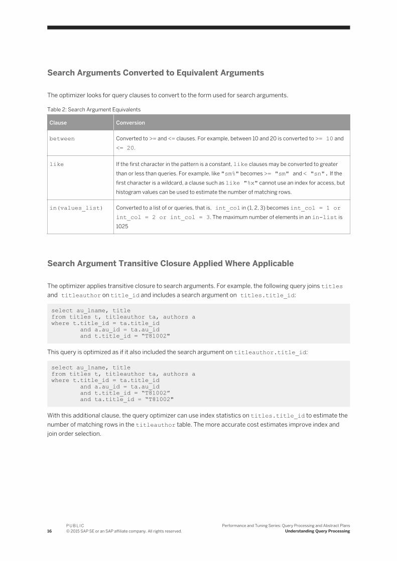
The optimizer looks for query clauses to convert to the form used for search arguments.
Table 2: Search Argument Equivalents
Clause Conversion
between Converted to >= and <= clauses. For example, between 10 and 20 is converted to >= 10 and <= 20.
like If the first character in the pattern is a constant, like clauses may be converted to greater than or less than queries. For example, like "sm%" becomes >= "sm" and < "sn". If the first character is a wildcard, a clause such as like "%x" cannot use an index for access, but histogram values can be used to estimate the number of matching rows.
in(values_list) Converted to a list of or queries, that is, int_col in (1, 2, 3) becomes int_col = 1 or int_col = 2 or int_col = 3. The maximum number of elements in an in-list is 1025
Search Argument Transitive Closure Applied Where Applicable
The optimizer applies transitive closure to search arguments. For example, the following query joins titles and titleauthor on title_id and includes a search argument on titles.title_id:
select au_lname, title from titles t, titleauthor ta, authors awhere t.title_id = ta.title_id and a.au_id = ta.au_id and t.title_id = “T81002"
This query is optimized as if it also included the search argument on titleauthor.title_id:
select au_lname, title from titles t, titleauthor ta, authors awhere t.title_id = ta.title_id and a.au_id = ta.au_id and t.title_id = “T81002” and ta.title_id = “T81002"
With this additional clause, the query optimizer can use index statistics on titles.title_id to estimate the number of matching rows in the titleauthor table. The more accurate cost estimates improve index and join order selection.
16P U B L I C© 2015 SAP SE or an SAP affiliate company. All rights reserved.
Performance and Tuning Series: Query Processing and Abstract PlansUnderstanding Query Processing

Equijoin Predicate Transitive Closure Applied Where Applicable
The optimizer applies transitive closure to join columns for a normal equi-join. The following query specifies the equi-join of t1.c11 and t2.c21, and the equi-join of t2.c21 and t3.c31:
select * from t1, t2, t3where t1.c11 = t2.c21 and t2.c21 = t3.c31 and t3.c31 = 1
Without join transitive closure, the only join orders considered are (t1, t2, t3), (t2, t1, t3), (t2, t3, t1),and (t3, t2, t1). By adding the join on t1.c11 = t3.31, the query processor expands the list of join orders to include: (t1, t3, t2) and (t3, t1, t2). Search argument transitive closure applies the condition specified by t3.c31 = 1 to the join columns of t1 and t2.
Similarly, equi-join transitive closure is also applied to equi-joins with or predicates as follows:
select * from R,S where R.a = S.a and (R.a = 5 OR S.b = 6)
The query optimizer infers that this would be equivalent to:
select * from R,S where R.a = S.a and (S.a = 5 or S.b = 6)
The or predicate could be evaluated on the scan of S and possibly be used for an or optimization, thereby effectively using the indexes of S.
Another example of join transitive closure is its application to complex SARGs, so that a query such as:
select * from R,S where R.a = S.a and (R.a + S.b = 6)
is transformed and inferred as:
select * from R,S where R.a = S.a and (S.a + S.b = 6)
The complex predicate could be evaluated on the scan of S, resulting in significant performance improvements due to early result set filtering.
Transitive closure is used only for normal equi-joins, as shown. join transitive closure is not performed for:
● Non-equi-joins; for example, t1.c1 > t2.c2● Outer joins; for example, t1.c11 *= t2.c2, or left join or right join● Joins across subquery boundaries● Joins used to check referential integrity or the with check option on views
Performance and Tuning Series: Query Processing and Abstract PlansUnderstanding Query Processing
P U B L I C© 2015 SAP SE or an SAP affiliate company. All rights reserved. 17

NoteAs of SAP ASE 15.0, the sp_configure option to turn on or off join transitive closure and sort merge join is discontinued. Whenever applicable, join transitive closure is always applied in SAP ASE 15.0 and later.
Predicate Transformation and Factoring to Provide Additional Optimization Paths
Predicate transformation and factoring increases the number of choices available to the query processor. It adds optimizable clauses to a query by extracting clauses from blocks of predicates linked with or into clauses linked by and. The additional optimized clauses mean there are more access paths available for query execution. The original or predicates are retained to ensure query correctness.
During predicate transformation:
1. Simple predicates (joins, search arguments, and in lists) that are an exact match in each or clause are extracted. In the query in step 3, below, this clause matches exactly in each block, so it is extracted:
t.pub_id = p.pub_id
between clauses are converted to greater-than-or-equal and less-than-or-equal clauses before predicate transformation. The sample query uses between 15 in both query blocks (though the end ranges are different). The equivalent clause is extracted by step 1:
price >=15
2. Search arguments on the same table are extracted; all terms that reference the same table are treated as a single predicate during expansion. Both type and price are columns in the titles table, so the extracted clauses are:
(type = "travel" and price >=15 and price <= 30) or (type = "business" and price >= 15 and price <= 50)
3. in lists and or clauses are extracted. If there are multiple in lists for a table within a blocks, only the first is extracted. The extracted lists for the sample query are:
p.pub_id in (“P220”, “P583”, “P780”) or p.pub_id in (“P651", “P066", “P629”)
Since these steps can overlap and extract the same clause, duplicates are eliminated.Each generated term is examined to determine whether it can be used as an optimized search argument or a join clause. Only those terms that are useful in query optimization are retained.The additional clauses are added to the query clauses specified by the user.For example, all clauses optimized in this query are enclosed in the or clauses:
select p.pub_id, price from publishers p, titles twhere ( t.pub_id = p.pub_id
18P U B L I C© 2015 SAP SE or an SAP affiliate company. All rights reserved.
Performance and Tuning Series: Query Processing and Abstract PlansUnderstanding Query Processing

and type = “travel" and price between 15 and 30 and p.pub_id in (“P220", “P583", “P780") )or ( t.pub_id = p.pub_id and type = “business" and price between 15 and 50 and p.pub_id in (“P651", “P066", “P629") )
Predicate transformation pulls clauses linked with and from blocks of clauses linked with or, such as those shown above. It extracts only clauses that occur in all parenthesized blocks. If the example above had a clause in one of the blocks linked with or that did not appear in the other clause, that clause would not be extracted.
1.1.4 Handling Search Arguments and Useful Indexes
It is important that you distinguish between the where and having clause predicates that are used to optimize the query, and those that are used later during query processing to filter the returned rows.
You can use search arguments to determine the access path to data rows when a column in the where clause matches an index key. You can use the index to locate and retrieve the matching data rows. Once the row has been located in the data cache or has been read into the data cache from disk, any remaining clauses are applied.
For example, if the authors table has on an index on au_lname and another on city, either index can be used to locate the matching rows for this query:
select au_lname, city, state from authorswhere city = “Washington" and au_lname = “Catmull"
The query optimizer uses statistics, including histograms, the number of rows in the table, the index heights, and the cluster ratios for the index and data pages to determine which index provides the cheapest access. The index that provides the cheapest access to the data pages is chosen and used to execute the query, and the other clause is applied to the data rows once they have been accessed.
1.1.5 Nonequality Operators
The nonequality operators—<, >, and !=—require special consideration.
The query optimizer checks whether it should cover nonclustered indexes if the column is indexed, and uses a nonmatching index scan if an index covers the query. However, if the index does not cover the query, the table is accessed through a row ID lookup of the data pages during the index scan.
Performance and Tuning Series: Query Processing and Abstract PlansUnderstanding Query Processing
P U B L I C© 2015 SAP SE or an SAP affiliate company. All rights reserved. 19
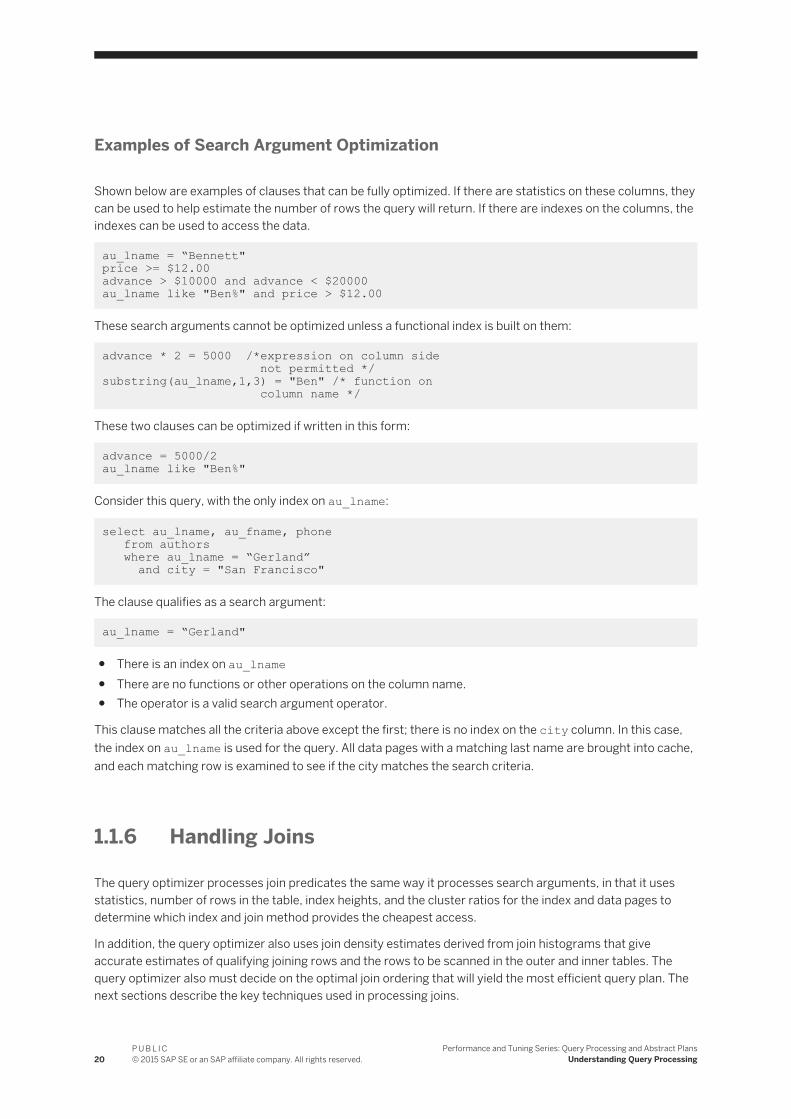
Examples of Search Argument Optimization
Shown below are examples of clauses that can be fully optimized. If there are statistics on these columns, they can be used to help estimate the number of rows the query will return. If there are indexes on the columns, the indexes can be used to access the data.
au_lname = “Bennett" price >= $12.00advance > $10000 and advance < $20000 au_lname like "Ben%" and price > $12.00
These search arguments cannot be optimized unless a functional index is built on them:
advance * 2 = 5000 /*expression on column side not permitted */substring(au_lname,1,3) = "Ben" /* function on column name */
These two clauses can be optimized if written in this form:
advance = 5000/2 au_lname like "Ben%"
Consider this query, with the only index on au_lname:
select au_lname, au_fname, phone from authors where au_lname = “Gerland” and city = "San Francisco"
The clause qualifies as a search argument:
au_lname = “Gerland"
● There is an index on au_lname● There are no functions or other operations on the column name.● The operator is a valid search argument operator.
This clause matches all the criteria above except the first; there is no index on the city column. In this case, the index on au_lname is used for the query. All data pages with a matching last name are brought into cache, and each matching row is examined to see if the city matches the search criteria.
1.1.6 Handling Joins
The query optimizer processes join predicates the same way it processes search arguments, in that it uses statistics, number of rows in the table, index heights, and the cluster ratios for the index and data pages to determine which index and join method provides the cheapest access.
In addition, the query optimizer also uses join density estimates derived from join histograms that give accurate estimates of qualifying joining rows and the rows to be scanned in the outer and inner tables. The query optimizer also must decide on the optimal join ordering that will yield the most efficient query plan. The next sections describe the key techniques used in processing joins.
20P U B L I C© 2015 SAP SE or an SAP affiliate company. All rights reserved.
Performance and Tuning Series: Query Processing and Abstract PlansUnderstanding Query Processing

Join Density and Join Histograms
The query optimizer uses a cost model for joins that uses table-normalized histograms of the joining attributes. This technique gives an exact value for the skewed values (that is, frequency count) and uses the range cell densities from each histogram to estimate the cell counts of corresponding range cells.
The join density is dynamically computed from the “join histogram,” which considers the joining of histograms from both sides of the join operator. The first histogram join occurs typically between two base tables when both attributes have histograms. Every histogram join creates a new histogram on the corresponding attribute of the parent join's projection.
The outcome of the join histogram technique is accurate join selectivity estimates, even if data distributions of the joining columns are skewed, resulting in superior join orders and performance.
Expression Histogramming Selectivity Estimates
Histogramming estimates are applied to single column predicates if the histogram exists on the column, resulting in more accurate row estimates, and improved join order selection for query plans. Versions earlier than 15.0.2 used default "guesses" for selectivity estimates.
In this example, if the expression is very selective, it may be better to place table t1 at the beginning of the join order:
select * from t1,t2 where substring(t1.charcol, 1, 3) = "LMC" and t1.a1 = t2.b
Joins with Mixed Datatypes
A basic requirement is for the ability to build keys for index lookups whenever possible, without regard to mixed datatypes of any of the join predicates versus the index key. Consider the following query:
create table T1 (c1 int, c2 int) create table T2 (c1 int, c2 float)create index i1 on T1(c2)create index i1 on T2(c2) select * from T1, T2 where T1.c2=T2.c2
Assume that T1.c2 is of type int and has an index on it, and that T2.c2 is of type float with an index.
As long as datatypes are implicitly convertible, the query optimizer can use index scans to process the join. In other words, the query optimizer uses the column value from the outer table to position the index scan on the inner table, even when the lookup value from the outer table has a different datatype than the respective index attribute of the inner table.
Performance and Tuning Series: Query Processing and Abstract PlansUnderstanding Query Processing
P U B L I C© 2015 SAP SE or an SAP affiliate company. All rights reserved. 21

Joins with Expressions and or Predicates
See Transformations for Query Optimization > Predicate Transformation and Factoring to Provide Additional Optimization Paths for description of how the query optimizer handles joins with expressions and or predicates.
Join Ordering
One of the key tasks of the query optimizer is to generate a query plan for join queries so that the order of the relations in the joins processed during query execution is optimal. This involves elaborate plan search strategies that can consume significant time and memory. The query optimizer uses several effective techniques to obtain the optimal join ordering. The key techniques are:
● Use of a greedy strategy to obtain an initial good ordering that can be used as an upper boundary to prune out other, subsequent join orderings. The greedy strategy employs join row estimates and the nested-loop-join method to arrive at the initial ordering.
● An exhaustive ordering strategy follows the greedy strategy. In this strategy, a potentially better join ordering replaces the join ordering obtained in the greedy strategy. This ordering may employ any join method.
● Use of extensive cost-based and rule-based pruning techniques eliminates undesirable join orders from consideration. The key aspect of the pruning technique is that it always compares partial join orders (the prefix of a potential join ordering) against the best complete join ordering to decide whether to proceed with the given prefix. This significantly improves the time required determine an optimal join order.
● The query optimizer can recognize and process star or snowflake schema joins and process their join ordering in the most efficient way. A typical star schema join involves a large Fact table that has equi-join predicates that join it with several Dimension tables. The Dimension tables have no join predicates connecting each other; that is, there are no joins between the Dimension tables themselves, but there are join predicates between the Dimension tables and the Fact table. The query optimizer employs special join ordering techniques during which the large Fact table is pushed to the end of the join order and the Dimension tables are pulled up front, yielding highly efficient query plans. The query optimizer does not, however, use this technique if the star schema joins contain subqueries, outer joins, or or predicates.
1.2 Optimization Goals
Use optimization goals to match query demands with the best optimization techniques, thus ensuring optimal use of the optimizer’s time and resources.
The query optimizer allows you to configure three types of optimization goals, which you can specify at three tiers: server level, session level, and query level.
Set the optimization goal at the desired level. The server-level optimization goal is overridden at the session level, which is overridden at the query level.
These optimization goals allow you to choose an optimization strategy that best fits your query environment:
22P U B L I C© 2015 SAP SE or an SAP affiliate company. All rights reserved.
Performance and Tuning Series: Query Processing and Abstract PlansUnderstanding Query Processing

● allrows_mix – the default goal, and the most useful goal in a mixed-query environment. allows_mix balances the needs of OLTP and DSS query environments.
● allrows_dss – the most useful goal for operational DSS queries of medium to high complexity. Currently, this goal is provided on an experimental basis.
● allrows_oltp – the optimizer considers only nested-loop joins.
At the server level, use sp_configure. For example:
sp_configure "optimization goal", 0, "allrows_mix"
At the session level, use set plan optgoal. For example:
set plan optgoal allrows_dss
At the query level, use a select or other DML command. For example:
select * from A order by A.a plan "(use optgoal allrows_dss)"
In general, you can set query-level optimization goals using select, update, and delete statements. However, you cannot set query-level optimization goals in pure insert statements, although you can set optimization goals in insert…select statements.
1.2.1 Limiting the Time Spent Optimizing a Query
Long-running and complex queries can be time consuming and costly to optimize. The timeout mechanism helps limit the time investment, while supplying a satisfactory query plan.
Context
The query optimizer provides a mechanism by which the optimizer can limit the time taken by long-running and complex queries; timing out allows the query processor to stop optimizing when it is reasonable to do so.
The optimizer triggers timeout during optimization when both these circumstances are met:
● At least one complete plan has been retained as the best plan, and● The user configured timeout percentage limit has been exceeded.
You can limit the amount of time SAP ASE spends optimizing a query at every level, using the optimization timeout limit parameter, which you can set to any value between 0 and 1000. optimization timeout limit represents the percentage of estimated query execution time that SAP ASE must spend to optimize the query. For example, specifying a value of 10 tells SAP ASE to spend 10% of the estimated query execution time in optimizing the query. Similarly, a value of 1000 tells SAP ASE to spend 1000% of the estimated query execution time, or 10 times the estimated query execution time, in optimizing the query.
See System Administration Guide, Volume 1 > Setting Configuration Parameters for more information about optimization timeout limit.
Performance and Tuning Series: Query Processing and Abstract PlansUnderstanding Query Processing
P U B L I C© 2015 SAP SE or an SAP affiliate company. All rights reserved. 23

A large timeout value may be useful for optimization of stored procedures with complex queries. Generally, longer optimization time of the stored procedures yields better plans; the longer optimization time can be amortized over several executions of the stored procedure.
A small timeout value may be used when you want a faster compilation time from complex ad hoc queries that normally take a long time to compile. However, for most queries, the default timeout value of 10 should suffice.
Procedure
Use sp_configure to set the optimization timeout limit configuration parameter at the server level. For example, to limit optimization time to 10% of total query processing time, enter:
sp_configure “optimization timeout limit", 10
Use set to set timeout at the session level:
set plan opttimeoutlimit <<n>>
where <n> is any integer between 0 and 4000.
Use select to limit optimization time at the query level:
select * from <<table>> plan "(use opttimeoutlimit <<n>>)"
<where n> is any integer between 0 and 1000.
1.3 Parallelism
SAP ASE supports horizontal and vertical parallelism for query execution. Vertical parallelism is the ability to run multiple operators at the same time by employing different system resources such as CPUs, disks, and so on. Horizontal parallelism is the ability to run multiple instances of an operator on the specified portion of the data.
See System Administration Guide, Volume 1 > Setting Configuration Parameters for a more detailed discussion of parallel query optimization in SAP ASE.
1.4 Optimization Issues
Although the query optimizer can efficiently optimize most queries, various issues may affect the optimizer’s efficiency.
Including:
● If statistics have not been updated recently, the actual data distribution may not match the values used to optimize queries.
24P U B L I C© 2015 SAP SE or an SAP affiliate company. All rights reserved.
Performance and Tuning Series: Query Processing and Abstract PlansUnderstanding Query Processing

● The rows referenced by a specified transaction may not fit the pattern reflected by the index statistics.● An index may access a large portion of the table.● where clauses (search arguments or SARGS) are written in a form that cannot be optimized.● No appropriate index exists for a critical query.● A stored procedure was compiled before significant changes to the underlying tables were performed.● No statistics exists for the SARG or joining columns.
These situations highlight the need to follow some best practices that allow the query optimizer to perform at its full potential:
Creating Search Arguments
Follow these guidelines when you write search arguments for your queries:
● Avoid functions, arithmetic operations, and other expressions on the column side of search clauses. When possible, move functions and other operations to the expression side of the clause.
● Use as many search arguments as you can, to give the query processor as much as possible to work with.● If a query has more than 400 predicates for a table, put the most potentially useful clauses near the
beginning of the query, since only the first 102 SARGs on each table are used during optimization. (All of the search conditions are used to qualify the rows.)
● Queries using > (greater than) may perform better if you can rewrite them to use >= (greater than or equal to). For example, this query, with an index on int_col, uses the index to find the first value where int_col equals 3, and then scans forward to find the first value that is greater than 3. If there are many rows where int_col equals 3, the server must scan many pages to find the first row where int_col is greater than 3:
select * from table1 where int_col > 3
It is more efficient to write the query this way:
select * from table1 where int_col >= 4
This optimization is more difficult with character strings and floating-point data.● Check the showplan output to see which keys and indexes are used.● If an index is not being used when you expect it to be, use output from the set commands in Table 3-1 on
page 114 to see whether the query processor is considering the index.
SQL Derived Tables
Queries expressed as a single SQL statement exploit the query processor better than queries expressed in two or more SQL statements.
SQL-derived tables enable you to express, in a single step, what might otherwise require several SQL statements and temporary tables, especially where intermediate aggregate results must be stored. For example:
select dt_1.* from
Performance and Tuning Series: Query Processing and Abstract PlansUnderstanding Query Processing
P U B L I C© 2015 SAP SE or an SAP affiliate company. All rights reserved. 25

(select sum(total_sales) from titles_west group by total_sales) dt_1(sales_sum), (select sum(total_sales) from titles_east group by total_sales) dt_2(sales_sum) where dt_1.sales_sum = dt_2.sales_sum
Here, aggregate results are obtained from the SQL derived tables dt_1 and dt_2, and a join is computed between the two SQL derived tables. Everything is accomplished in a single SQL statement.
See Transact-SQL Users Guide > SQL Derived Tables.
Tuning According to Object Sizes
To understand query and system behavior, know the sizes of your tables and indexes.
At several stages of tuning work, you need size data to:
● Understand statistics i/o reports for a specific query plan.● Understand the query processor's choice of query plan. The SAP ASE cost-based query processor
estimates the physical and logical I/O required for each possible access method and selects the cheapest method.
● Determine object placement, based on the sizes of database objects and on the expected I/O patterns on the objects.To improve performance, distribute database objects across physical devices, so that reads and writes to disk are evenly distributed.Object placement is described in the Performance and Tuning Series: Physical Database Tuning.
● Understand changes in performance. If objects grow, their performance characteristics can change. For example, consider a table that is heavily used and is usually 100 percent cached. If the table grows too large for its cache, queries that access the table can suffer poor performance. This is particularly true of joins that require multiple scans.
● Do capacity planning. Whether you are designing a new system or planning for the growth of an existing system, you must know the space requirements to plan for physical disks and memory needs.
● Understand output from sp_sysmon reports on physical I/O.
See the System Administration Guide: Volume 2 for more information on sizing.
1.5 Lava Query Execution Engine
In SAP ASE, all query plans are submitted to the procedural execution engine for execution.
The procedural execution engine drives execution of the query plan by:
● Executing simple SQL statements such as set, while, and goto directly.● Calling out to the utility modules of the query plan to execute create table and create index and
other utility commands.● Setting up the context for and driving the execution of stored procedures and triggers.
26P U B L I C© 2015 SAP SE or an SAP affiliate company. All rights reserved.
Performance and Tuning Series: Query Processing and Abstract PlansUnderstanding Query Processing

● Setting up the execution context and calling the query execution engine to execute query plans for select, insert, delete, and update statements.
● Setting up the cursor execution context for cursor open, fetch, and close statements, and calling the query execution engine to execute these statements.
● Doing transaction processing and post execution cleanup.
The procedural execution engine in SAP ASE 15.0 and later passes all query plans generated by the new query optimizer to the lava query execution engine.
The lava query execution engine executes lava query plans. All query plans chosen by the optimizer are compiled into lava query plans. However, SQL statements that are not optimized, such as set or create, are compiled into query plans like those in versions of SAP ASE earlier than 15.0, and are not executed by the lava query execution engine. Non-lava query plans are either executed by the procedural execution engine or by utility modules called by the procedural engine. SAP ASE version 15.0 and later has two distinct kinds of query plans and this is clearly seen in the showplan output..
Related Information
Displaying Query Optimization Strategies and Estimates [page 103]
1.5.1 Lava Query Plans
A lava query plan is built as an upside down tree of lava operators: the top lava operator can have one or more child operators, which in turn can have one or more child operators, and so on, thus building a bottom-up tree of operators.
The exact shape of the tree and the operators in it are chosen by the optimizer.
Below is an example of a lava query plan for this query:
Select o.id from sysobjects o, syscolumns c where o.id <= 1 and o.id < 2
Performance and Tuning Series: Query Processing and Abstract PlansUnderstanding Query Processing
P U B L I C© 2015 SAP SE or an SAP affiliate company. All rights reserved. 27

The lava query plan for this query consists of four lava operators. The top operator is an Emit (also called Root) operator that dispatches the results of query execution either by sending the rows to the client or by assigning values to local variables.
The only child operator of the Emit is a NestedLoopJoin (NL Join) that uses the nested loop join algorithm to join the rows coming from its two child operators:
● The scan of sysobjects● The scan of syscolumns
Since the optimizer optimizes all select, insert, delete and update statements, these are always compiled into lava query plans and executed by the lava query engine.
Some SQL statements are compiled into hybrid query plans. Such plans have multiple steps, some of which are executed by the Utility modules, and a final step that is a lava query plan. An example is the select into statement; select into is compiled into a two-step query plan:
● create table creates the target table of the statement.● A lava query plan to inserts the rows into the target table. To execute this query plan, the Procedural
Execution Engine calls the create table utility to execute the first step to create the table.
Then the procedural engine calls the lava query execution engine to execute the lava query plan to select and insert the rows into the target table.
The two other SQL statements that generate hybrid query plans are alter table (but only when data copying is required) and reorg rebuild.
The bcp utility generates a lava query plan and calls the lava query execution engine to execute the plan.
1.5.1.1 Lava Query Execution
Execution of a lava query plan involves five phases.
Each lava operator has a method with the same name as the phase, which is invoked for each of these phases.
The phases of query plan execution are:
Phase Description
Acquire Acquires resources needed for execution, such as memory buffers and creating worktables.
Invokes the acquire method of the Emit operator. The Emit operator calls Acquire of its child, the NLJoin operator, which in turn calls Acquire on its left-child operator (the index scan of sysobjects) and then on its right child operator (the index scan of syscolumns).
Open Invokes the Open method of the Emit operator. The Emit operator calls Open on the NLJoin operator, which calls Open only on its left-child operator.
Next Generates the next result row.
Invokes the Next method of the Emit operator. Emit calls Next on the NLJoin operator, which calls Next on its left child, the Index Scan of sysobjects. The index scan operator reads the first row
28P U B L I C© 2015 SAP SE or an SAP affiliate company. All rights reserved.
Performance and Tuning Series: Query Processing and Abstract PlansUnderstanding Query Processing

Phase Description
from sysobjects and returns it to the NLJoin operator. The NLJoin operator then calls the Open method of its right child operator, the Index Scan of syscolumns. Then the NLJoin operator calls the Next method of the Index Scan of syscolumns to get a row that matches the joining key of the row from sysobjects. When a matching row has been found, it is returned to the Emit operator, which sends it back to the client. Repeated invocations of the Next method of the Emit operator generate more result rows.
Close Cleans up; for example, notifies the access layer that scanning is complete or truncates worktables
After all rows have been returned, invokes the Close method of the Emit operator, which in turn calls Close of the NLJoin operator, which in turn calls Close on both of its child operators.
Release Releases resources acquired during Acquire, such as memory buffers, drops worktables.
Invokes the Release method of the Emit operator is invoked and the calls to the Release method of the other operators is propagated down the query plan.
1.5.1.2 Lava Operators
Lava query plans are built of lava operators. Each lava operator is a self-contained software object that implements one of the basic physical operations that the optimizer uses to build query plans.
Each lava operator has five methods that can be called by its parent operator. These five methods correspond to the five phases of query execution:
● Acquire● Open● Next● Close● Release
Because the lava operators all provide the same methods (that is, the same API), they can be interchanged like building blocks in a lava query plan. For example, you can replace the NLJoin operator with a MergeJoin operator or a HashJoin operator without impacting any of the other three operators in the query plan.
The lava operators that can be chosen by the optimizer to build lava query plans are listed below:
Operator Description
BulkOp Executes the part of bcp processing that is done in the lava query engine. Only found in query plans that are created by the bcp utility, not those created by the optimizer.
CacheScanOp Reads rows from an in-memory table.
DelTextOp Deletes text page chains as part of alter table drop column processing.
Performance and Tuning Series: Query Processing and Abstract PlansUnderstanding Query Processing
P U B L I C© 2015 SAP SE or an SAP affiliate company. All rights reserved. 29

Operator Description
DeleteOp Deletes rows from a local table.Deletes rows from a proxy table when the entire SQL statement cannot be shipped to the remote server. See also RemoteScanOp.
EmitOp (RootOp) Routes query execution result rows. Can send results to the client or assign result values to local variables or fetch into variables. An EmitOp is always the top operator in a lava query plan.
EmitExchangeOp Routes result rows from a subplan that is executed in parallel to the ExchangeOp in the parent plan fragment. EmitExchangeOp always appears directly under an ExchangeOp. See Parallel Query Processing [page 125].
GroupSortedOp (Aggregation)
Performs vector aggregation (group by) when the input rows are already sorted on the group-by columns. See also HashVectorAggOp.
GroupSorted (Distinct) Eliminates duplicate rows. Requires the input rows to be sorted on all columns. See also HashDistinctOp and SortOp (Distinct).
HashVectorAggOp Performs vector aggregation (group by). Uses a Hash algorithm to group the input rows, so no requirements on ordering of the input rows. See also GroupSortedOp (Aggregation).
HashDistinctOp Eliminates duplicate rows using a hashing algorithm to find duplicate rows. See also GroupSortedOp (Distinct) and SortOp (Distinct).
HashJoinOp Performs a join of two input row streams using the HashJoin algorithm.
HashUnionOp Performs a union operation of two or more input row streams using a hashing algorithm to find and eliminate duplicate rows. See also MergeUnionOp and UnionAllOp.
InsScrollOp Implements extra processing needed to support insensitive scrollable cursors. See also SemiInsScrollOp.
InsertOp Inserts rows to a local table.Inserts rows to a proxy table when the entire SQL statement cannot be shipped to the remote server. See also RemoteScanOp.
MergeJoinOp Performs a join of two streams of rows that are sorted on the joining columns using the mergejoin algorithm.
MergeUnionOp Performs a union or union all operation on two or more sorted input streams. Guarantees that the output stream retains the ordering of the input streams. See also HashUnionOp and UnionAllOp.
NestedLoopJoinOp Performs a join of two input streams using the NestedLoopJoin algorithm.
NaryNestedLoopJoinOp Performs a join of three or more input streams using an enhanced NestedLoopJoin algorithm. This operator replaces a left-deep tree of
30P U B L I C© 2015 SAP SE or an SAP affiliate company. All rights reserved.
Performance and Tuning Series: Query Processing and Abstract PlansUnderstanding Query Processing

Operator Description
NestedLoopJoin operators and can lead to significant performance improvements when rows of some of the input streams can be skipped.
OrScanOp Inserts the in or or values into an in-memory table, sorts the values, and removes the duplicates.Then returns the values, one at a time. Only used for SQL statements with in clauses or multiple or clauses on the same column.
PtnScanOp Reads rows from a local table (partitioned or not) using either a table scan or an index scan to access the rows.
RIDJoinOp Receives one or more row identifiers (RIDs) from its left-child operator and calls on its right-child operator (PtnScanOp) to find the corresponding rows. Used only on SQL statements with or clauses on different columns of the same table.
RIFilterOp (Direct) Drives the execution of a subplan to enforce referential integrity constraints that can be checked on a row-by-row basis.Appears only in insert, delete, or update queries on tables with referential integrity constraints.
RIFilterOp (Deferred) Drives the execution of a sub-plan to enforce referential integrity constraints that can only be checked after all rows that are affected by the query have been processed.
RemoteScanOp Accesses proxy tables. The RemoteScanOp can:
● Read rows from a single proxy table for further processing in a lava query plan on the local host.
● Pass complete SQL statements to a remote host for execution: insert, delete, update, and select statements. In this case, the lava query plan consists of an EmitOp with a RemoteScanOp as its only child operator.
● Pass an arbitrarily complex query plan fragment to a remote host for execution and read in the result rows (function shipping).
RestrictOp Evaluates expressions.
SQFilterOp Drives the execution of a subplan to execute one or more subqueries.
ScalarAggOp Performs scalar aggregation, such as aggregates without group by.
SemiInsScrollOp Performs extra processing to support semi-insensitive scrollable cursors. See also InsScrollOp.
SequencerOp Enforces sequential execution of different sub-plans in the query plan.
SortOp Sorts its input rows based upon specified keys.
SortOp (Distinct) Sorts its input and removes duplicate rows. See also HashDisitnctOp and GroupSortedOp (Distinct).
Performance and Tuning Series: Query Processing and Abstract PlansUnderstanding Query Processing
P U B L I C© 2015 SAP SE or an SAP affiliate company. All rights reserved. 31

Operator Description
StoreOp Creates and coordinates the filling of a worktable, and creates a clustered index on the worktable if required. StoreOp can only have an InsertOp as a child; the InsertOp populates the worktable.
UnionAllOp Performs a union all operation on two or more input streams. See also HashUnionOp and MergeUnionOp.
UpdateOp Changes the value of columns in rows of a local table or of a proxy table when the entire update statement cannot be sent to the remote server. See also RemoteScanOp.
ExchangeOp Enables and coordinates parallel execution of lava query plans. The ExchangeOp can be inserted between almost any two lava operators in a query plan to divide the plan into sub-plans that can be executed in parallel. See Parallel Query Processing.
1.5.1.3 Simplified Native Access Plans on Linux
SAP ASE on Linux includes an additional, just-in-time compilation phase that, when enabled, compiles lava execution plans into native code. This native plan feature is available as part of the MemScale licensed option.
This feature is available for nonclustered SAP ASE servers on Linux x86-64/amd64, running in threaded-kernel mode, when you enable it using the simplified native access plan configuration parameter to enable this feature. See simplified native access plan (Linux Only) in the System Administration Guide Volume 1.
Simplified native access plans are transparent to the user. When enabled, SAP ASE uses simplified native access plans whenever qualified plans are available.
This feature supports:
● Statement cache plans, including those used for dynamic SQL (prepared statements).● Plans with user stored procedures.
The second time you execute an ad hoc query-cached lava plan or the first time you execute a lava plan in a user stored procedure/dynamic prepared statement, SAP ASE examines the plan and generates an intermediate representation (IR) of its simplified native access plan. This IR program is then compiled into a native code function, which, when invoked, produces the same result as the original lava plan.
The primary advantage for converting lava plans into simplified native access plans is that invoking these native code plans directly allows SAP ASE to execute extreme online transaction processing (XOLTP) queries much more rapidly
When enabled, this feature runs automatically on any lava plan-based Transact-SQL command, depending on the query plan type and table type used in the execution. Lava query plans supported for native code compilation are:
● Statement cache plans, including those used for dynamic SQL (prepared statements).● Plans with user stored procedures.
32P U B L I C© 2015 SAP SE or an SAP affiliate company. All rights reserved.
Performance and Tuning Series: Query Processing and Abstract PlansUnderstanding Query Processing

● Datarows locking table/index serial scan, with optional dynamic partition elimination● Scan and PtnScan (partition acan) sperators● Restrict operator● Emit operator, including EmitSndOp and EmitNoSndOp● OrScan operator● Nested loop join operator without worktable usage (for example, no reformatting)● NaryNLJ operator● Scalar aggregate operator● insert, update, delete operator● union all operator● ScalarOp operator
Unsupported lava plans continue to execute using the lava execution engine; the process is transparent to user. In addition to such unsupported plans (that is, those not listed in the list above), plans with the following operations are also not supported by the simplified native access plan feature:
● Cursors● RID scan● LOB datatype● Remote tables● Parallel plans● The compute clause● Versions of TDS, the server/client communication protocol used by ASE, lower than 5● Java datatypes● Precomputed result sets or materialized views● SQL replication● Bulk insert● instead of triggers● select for update● All-pages lock and data-page lock● Nested SQL● merge statement● NetScan● Outer joins● Sort operator● Sequencer operator● User-defined function● RID join operator● Hash join operator● Merge join operator● Merge union operator● Update index operator● Store and StoreIndex operator● BloomFilter operator● Referential Integrity● SQFilter operator
Performance and Tuning Series: Query Processing and Abstract PlansUnderstanding Query Processing
P U B L I C© 2015 SAP SE or an SAP affiliate company. All rights reserved. 33

● GroupSort operator● AMC query● Identity and timestamp column exist
1.5.1.3.1 Disable ASLR
Disable the Address Space Layout Randomization (ASLR) feature on Linux before enabling simplified native access plans.
Context
When Address Space Layout Randomization is enabled, the SAP ASE cannot communicate over the shared memory segment with the compile server for generated code sections. When you try to generate a simplified native access plan without disabling ASLR, you see a message similar to:
kernel PCI(M1): ERROR: llvmcs_bootstrap; PCI Bridge can not interact with LLVMCS over randomized address space (see your platform kernel.randomize_va_space).
See your Linux operating system documentation for more information on ASLR and the kernel.randomize_va_space setting.
Perform the following to turn all randomization off in your system.
Procedure
1. Edit the /etc/sysctl.conf file to include the following line:
kernel.randomize_va_space=0
2. For the action to take effect, log in as the super user (root) and enter:
/sbin/sysctl -p
1.5.1.3.2 Enabling SNAPs
Enable configuration parameters to use simplified native access plans.
See System Administration Guide: Volume 1 > Setting Configuration Parameters for details on configuration parameters..
34P U B L I C© 2015 SAP SE or an SAP affiliate company. All rights reserved.
Performance and Tuning Series: Query Processing and Abstract PlansUnderstanding Query Processing

Parameter Description
enable mem scale
The MemScale option is a licensed option introduced in SAP ASE version 16.0 SP02 as part of the SQL Server Administration group.
Turning the sp_config enable mem scale option on enables all of the features included in the ASE_MEMSCALE license, including the Simplified Native Access Plan feature:
sp_configure "enable mem scale", 1
When you enable an individual feature that is part of the MemScale option, the license manager verifies that you have the ASE_MEMSCALE license, and that you have enabled the enable mem scale option.
streamlined dynamic SQL
Enable the streamlined dynamic SQL configuration parameter:
sp_configure "streamlined dynamic SQL", 1
This parameter enables the statement cache to store dynamic SQL statements.
NoteEnable this parameter even if you are not using dynamic SQL.
enable pci Enable the PCI Bridge for SAP ASE
SAP ASE requires the sybpcidb database when you enable PCI Bridge, as it contains all the configuration data for PCI Bridge and its associated pluggable component adaptors (PCAs). There are, however, no separate entries to add to sybpcidb to use simplified native access plans.
To enable PCI Bridge:
1. As system administrator, create the sybpcidb database using the srvbuild or sybconfig installation and configuration utilities, or by running the $SYBASE/$SYBASE_ASE/scripts/installpcidb script. See the SAP ASE Installation Guide > Managing Java in the Database During Installations and Upgrades for details.
2. Enable PCI Bridge:
sp_configure 'enable pci', 1
3. Restart SAP ASE.When SAP ASE brings up the compile server, you see a message similar to the following from the kernel, in either the SAP ASE errorlog, or the SAP ASE console output:Bootstrapping LLVM Compile Server [llvmcs] – Compile Server process running PID xxxxx
simplified native access plan
Set the simplified native access plan configuration plan to 1:
sp_configure "simplified native access plan", 1
The default is 0 (zero), which disables the feature. The configuration parameter is dynamic; you do not need to restart SAP ASE.
Performance and Tuning Series: Query Processing and Abstract PlansUnderstanding Query Processing
P U B L I C© 2015 SAP SE or an SAP affiliate company. All rights reserved. 35

statement cache size
To use simplified native access plans with statement cache plans (including dynamic SQL), activate the statement cache by setting the statement cache size configuration parameter to the size of the cache in 2K pages (the default value is 0). See System Administration Guide Volume 2 > Configuring Memory > The Statement Cache for details on the statement cache.
You need not enable this parameter if you only plan to use SNAP with user-stored procedures.
1.5.1.3.3 SNAPs and the Compile Server
To maintain complete separation between the SAP ASE dataserver process and the compilation process that happens for the Simplified Native Access Plan feature, SAP ASE bring up a separate operating system process called "compile server."
The new feature uses a compile server to generate the native code for SNAP.
The compile server is transparent to the user; you do not need to enable any configuration for it to run.
With the SNAP feature enabled, the SAP ASE server brings up and monitors the compile server. When necessary, SAP ASE server resets the compile server to keep it in a healthy state.
Whenever the compile server is not available momentarily, any new SNAP automatically falls back to the original lava query plan execution.
1.5.1.3.4 Checking Whether a Plan is a Candidate for SNAP
Use the output from showplan to determine whether a plan can be used with the Simplified Native Access Plan feature.
To verify whether a plan is a candidate for SNAP, use showplan. You see output similar to the following:
use tempdb gocreate table t1(c1 int) lock datarowsgoset showplan ongoselect * from t1goQUERY PLAN FOR STATEMENT 1 (at line 1). STEP 1 The type of query is EXECUTE. Executing a newly cached statement (SSQL_ID = 849326342).QUERY PLAN FOR STATEMENT 1 (at line 1).Optimized using Serial ModeTo be prepared at runtime using simplified native access plan. STEP 1 The type of query is SELECT. 1 operator(s) under root |ROOT:EMIT Operator (VA = 1) | | |SCAN Operator (VA = 0)
36P U B L I C© 2015 SAP SE or an SAP affiliate company. All rights reserved.
Performance and Tuning Series: Query Processing and Abstract PlansUnderstanding Query Processing

| | FROM TABLE | | t1 | | Table Scan. | | Forward Scan. | | Positioning at start of table. | | Using I/O Size 16 Kbytes for data pages. | | With LRU Buffer Replacement Strategy for data pages. c1 ----------- (0 rows affected)1> select * from t12> goQUERY PLAN FOR STATEMENT 1 (at line 1). STEP 1 The type of query is EXECUTE. Executing a previously cached statement (SSQL_ID = 849326342).QUERY PLAN FOR STATEMENT 1 (at line 1).Optimized using Serial ModeTo be prepared at runtime using simplified native access plan. STEP 1 The type of query is SELECT. 1 operator(s) under root |ROOT:EMIT Operator (VA = 1) | | |SCAN Operator (VA = 0) | | FROM TABLE | | t1 | | Table Scan. | | Forward Scan. | | Positioning at start of table. | | Using I/O Size 16 Kbytes for data pages. | | With LRU Buffer Replacement Strategy for data pages. c1 ----------- (0 rows affected)1> set statistics plancost on2> goQUERY PLAN FOR STATEMENT 1 (at line 1). STEP 1 The type of query is SET STATISTICS ON.1> select * from t12> goQUERY PLAN FOR STATEMENT 1 (at line 1). STEP 1 The type of query is EXECUTE. Executing a previously cached statement (SSQL_ID = 849326342).QUERY PLAN FOR STATEMENT 1 (at line 1).Optimized using Serial ModePrepared at runtime using simplified native access plan. STEP 1 The type of query is SELECT. 1 operator(s) under root |ROOT:EMIT Operator (VA = 1) | | |SCAN Operator (VA = 0) | | FROM TABLE | | t1 | | Table Scan. | | Forward Scan. | | Positioning at start of table. | | Using I/O Size 16 Kbytes for data pages. | | With LRU Buffer Replacement Strategy for data pages.========== Executed using Simplified Native Access Plan ====================================================================== c1 ----------- (0 rows affected) 1>
Performance and Tuning Series: Query Processing and Abstract PlansUnderstanding Query Processing
P U B L I C© 2015 SAP SE or an SAP affiliate company. All rights reserved. 37

For a candidate plan, depending on whether SNAP generation has been started, showplan prints these additional messages:
● When a candidate plan is first being executed:
To be prepared at runtime using simplified native access plan.
● When a candidate plan has started its SNAP generation and its just-in-time compilation:
Prepared at runtime using simplified native access plan.
NoteThis message, however, does not indicate whether the simplified native access plan is ready, or whether it is being used for the current execution.
To verify whether a simplified native access plan was ready and is indeed being used for the current execution, view the contents from set statistics plancost on. Instead of a header indicating lava exec statistics, you see:
========= Executed using Simplified Native Access Plan =========
If SAP ASE cannot generate a simplified native access plan for a query plan, find out why by turning on trace flag 11886 at the session level. For example, this diagnostics message indicates that the query plan cannot generate SNAP because it includes compute clause:
"...snap_reasons=... (SNAP_REASON_COMPUTE)"
This example indicates that the query plan cannot execute SNAP because the session client's TDS version is lower than 5.0.0:
"...no_snap_exec, !FE_ROWFMT_OK"
1.5.1.3.5 Monitoring SNAPs on Linux
Use the monState and monCachedProcedures monitoring tables to obtain information about Simplified Native Access Plans.
The monState monitoring table includes these two columns:
Column Description
SnapsGenerated This column displays the number of simplified native access plans compiled since the SAP ASE server was last restarted.
SnapsExecuted This column displays the number of actual query plan executions using Simplified Native Access Plans since the SAP ASE server was last restarted.
For example, the following query can return the above added counter information:
select Selects+Updates+Deletes+Inserts+Merges as "Totals", SnapsGenerated, SnapsExecuted from master..monState
38P U B L I C© 2015 SAP SE or an SAP affiliate company. All rights reserved.
Performance and Tuning Series: Query Processing and Abstract PlansUnderstanding Query Processing

Since SnapsExecuted is a subset of the total number of query plans executed, by comparing the values between Totals and SnapsExecuted, you can see how frequently simplified native access plans have been used.
To enable these monState columns, set the enable monitoring configuration parameter to 1:
sp_configure "enable monitoring", 1
The monCachedProcedures monitoring table includes these four columns that allow you to obtain information about the generation and execution of individual SNAPs:
Column Description
SnapCodegenTime This column displays the total number of microseconds of CPU time used by the stored procedure plan's SNAP code generation for simplified native access plans.
SnapJITTime This column displays the total number of microseconds of CPU time used by the stored procedure plan's SNAP JIT compilation.
SnapExecutionTime This column displays the total accumulated amount of elapsed time, in microseconds, that the stored procedure plan's SNAP has executed across multiple procedure executions.
SnapExecutionCount This column displays the number of times the stored procedure plan's SNAP has executed.
If you use these counters in user stored procedures, the values are the accumulated numbers across multiple compiled queries within the same procedure.
For example, the following query can return the above added counter information:
select ExecutionCount as "Total Count", ExecutionTime as "Total Time", SnapCodegenTime, SnapJITTime, SnapExecutionTime, SnapExecutionCount from master..monCachedProcedures
To enable these monCachedProcedures columns, set these two configuration parameters:
● Set enable monitoring configuration parameter to 1:
sp_configure "enable monitoring", 1
● Set statement statistics active configuration parameter to 1:
sp_configure "statement statistics active", 1
1.5.1.3.6 Removing Plans and Stored Procedures
Remove SNAPs and stored procedures.
Context
Whenever SAP ASE removes the original lava query plan, its corresponding SNAP is also removed.
Performance and Tuning Series: Query Processing and Abstract PlansUnderstanding Query Processing
P U B L I C© 2015 SAP SE or an SAP affiliate company. All rights reserved. 39

Procedure
● To remove a generated SNAP for statement cached plans, use a purge command such as dbcc purgesqlplan.
● To remove user stored procedures, use the exec ... with recompile command.
1.6 Update Operations
SAP ASE handles updates in different ways, depending on data changes and the indexes used to locate the rows.
The two major types of updates are deferred updates and direct updates. SAP ASE performs direct updates whenever possible.
1.6.1 Direct Updates
SAP ASE performs direct updates in a single pass, by locating the affected index and data rows, writing records for the changes to the transaction log, and making the changes to affected data and index pages.
There are three techniques for performing direct updates:
● In-place updates● Cheap direct updates● Expensive direct updates
Direct updates require less overhead than deferred updates and are generally faster, as they limit the number of log scans, reduce logging, save traversal of index B-trees (reducing lock contention), and save I/O because SAP ASE does not have to refetch pages to perform modifications based on log records.
In-Place Updates
SAP ASE performs in-place updates whenever possible. Subsequent rows on the page are not moved; row IDs remain the same and the pointers in the row offset table are not changed.
For an in-place update, the following requirements must be met:
● The row being changed cannot change its length.● The column being updated cannot be the key, or part of the key, of a clustered index on an allpages-locked
table. Because the rows in a clustered index on an allpages-locked table are stored in key order, a change to the key almost always means that the row location is changed.
● One or more indexes must be unique or must allow duplicates.● The update statement satisfies the conditions listed in “Restrictions on update modes through joins” on
page 35.
40P U B L I C© 2015 SAP SE or an SAP affiliate company. All rights reserved.
Performance and Tuning Series: Query Processing and Abstract PlansUnderstanding Query Processing

● The affected columns are not used for referential integrity.● There cannot be a trigger on the column.● The table cannot be replicated (via Replication Server).
An in-place update is the fastest type of update because it makes a single change to the data page. It changes all affected index entries by deleting the old index rows and inserting the new index row. In-place updates affect only indexes whose keys are changed by the update, since the page and row locations are not changed.
Cheap Direct Updates
If SAP ASE cannot perform an update in place, it tries to perform a cheap direct update—changing the row and rewriting it at the same offset on the page.
Subsequent rows on the page are moved up or down so that data remains contiguous on the page, but row IDs remain the same. The pointers in the row offset table change to reflect the new locations.
A cheap direct update must meet these requirements:
● The length of the data in the row is changed, but the row still fits on the same data page, or the row length is not changed, but there is a trigger on the table or the table is replicated.
● The column being updated cannot be the key, or part of the key, of a clustered index. Because SAP ASE stores the rows of a clustered index in key order, a change to the key almost always means that the row location is changed.
● One or more indexes must be unique or must allow duplicates.● The update statement satisfies the conditions listed in “Restrictions on Update Modes Through Joins."● The affected columns are not used for referential integrity.
Cheap direct updates are almost as fast as in-place updates. They require the same amount of I/O, but slightly more processing. Two changes are made to the data page (the row and the offset table). Any changed index keys are updated by deleting old values and inserting new values. Cheap direct updates affect only indexes whose keys are changed by the update, since the page and row ID are not changed.
Expensive Direct Updates
If the data does not fit on the same page, SAP ASE performs an expensive direct update, if possible. An expensive direct update deletes the data row, including all index entries, and then inserts the modified row and index entries.
SAP ASE uses a table scan or an index to find the row in its original location and then deletes the row. If the table has a clustered index, SAP ASE uses the index to determine the new location for the row; otherwise, SAP ASE inserts the new row at the end of the heap.
An expensive direct update must meet these requirements:
● The length of a data row is changed so that the row no longer fits on the same data page, and the row is moved to a different page, or the update affects key columns for the clustered index.
● The index used to find the row is not changed by the update.● The update statement satisfies the conditions listed in “Restrictions on update modes through joins” on
page 35.
Performance and Tuning Series: Query Processing and Abstract PlansUnderstanding Query Processing
P U B L I C© 2015 SAP SE or an SAP affiliate company. All rights reserved. 41

● The affected columns are not used for referential integrity.
An expensive direct update is the slowest type of direct update. The delete is performed on one data page, and the insert is performed on a different data page. All index entries must be updated, since the row location is changed.
1.6.2 Deferred Updates
SAP ASE uses deferred updates when direct update conditions are not met. A deferred update is the slowest type of update.
In a deferred update, SAP ASE:
● Locates the affected data rows, writing the log records for deferred delete and insert of the data pages as rows are located.
● Reads the log records for the transaction and performs the deletes on the data pages and any affected index rows.
● Reads the log records a second time, and performs all inserts on the data pages, and inserts any affected index rows.
When Deferred Updates Are Required
Deferred updates are always required for certain updates.
Including:
● Updates that use self-joins● Updates to columns used for self-referential integrity● Updates to a table referenced in a correlated subquery
Deferred updates are also required when:
● An update moves a row to a new page while the table is being accessed by a table scan or a clustered index.
● Duplicate rows are not allowed in the table, and there is no unique index to prevent them.● The index used to find the data row is not unique, and the row is moved because the update changes the
clustered index key or because the new row does not fit on the page.
Deferred updates incur more overhead than direct updates because they require SAP ASE to reread the transaction log to make the final changes to the data and indexes. This involves additional traversal of the index trees.
For example, if there is a clustered index on title, this query performs a deferred update:
update titles set title = "Portable C Software" where title = "Designing Portable Software"
42P U B L I C© 2015 SAP SE or an SAP affiliate company. All rights reserved.
Performance and Tuning Series: Query Processing and Abstract PlansUnderstanding Query Processing

1.6.3 Deferred Index Inserts
SAP ASE performs deferred index updates when the update affects the index used to access the table or when the update affects columns in a unique index.
In this type of update, SAP ASE:
● Deletes the index entries in direct mode● Updates the data page in direct mode, writing the deferred insert records for the index● Reads the log records for the transaction and inserts the new values in the index in deferred mode
Deferred index insert mode must be used when the update changes the index used to find the row or when the update affects a unique index. A query must update a single, qualifying row only once—deferred index update mode ensures that a row is found only once during the index scan and that the query does not prematurely violate a uniqueness constraint.
The update described below changes only the last name, but the index row is moved from one page to the next. To perform the update, SAP ASE:
1. Reads index page 1133, deletes the index row for “Greene” from that page, and logs a deferred index scan record.
2. Changes “Green” to “Hubbard” on the data page in direct mode and continues the index scan to see if more rows need to be updated.
3. Inserts the new index row for “Hubbard” on page 1127.
This figure shows the index and data pages prior to the deferred update operation, and the sequence in which the deferred update changes the data and index pages.
Performance and Tuning Series: Query Processing and Abstract PlansUnderstanding Query Processing
P U B L I C© 2015 SAP SE or an SAP affiliate company. All rights reserved. 43

Assume a similar update to the titles table:
update titles set title = "Computer Phobic’s Manual", advance = advance * 2 where title like "Computer Phob%"
This query shows a potential problem. If a scan of the nonclustered index on the title column found “Computer Phobia Manual,” changed the title, and multiplied the advance by 2, and then found the new index row “Computer Phobic’s Manual” and multiplied the advance by 2, the advance wold be very skewed against the reality.
A deferred index delete may be faster than an expensive direct update, or it may be substantially slower, depending on the number of log records that need to be scanned and whether the log pages are still in cache.
44P U B L I C© 2015 SAP SE or an SAP affiliate company. All rights reserved.
Performance and Tuning Series: Query Processing and Abstract PlansUnderstanding Query Processing

During deferred update of a data row, there can be a significant time interval between the delete of the index row and the insert of the new index row. During this interval, there is no index row corresponding to the data row. If a process scans the index during this interval at isolation level 0, it does not return the old or new value of the data row.
1.6.4 Restrictions on Update Modes Through Joins
Updates and deletes that involve joins can be performed in direct, deferred_varcol, or deferred_index mode when the table being updated is the outermost table in the join order, or when it is preceded in the join order by tables in which only a single row qualifies.
Deletes and Updates in Triggers Versus Referential Integrity
Triggers that join user tables with the deleted or inserted tables are run in deferred mode.
If you are using triggers solely to implement referential integrity, and not to cascade updates and deletes, then using declarative referential integrity in place of triggers may avoid the penalty of deferred updates in triggers.
1.6.4.1 Joins and Subqueries in Update and Delete Statements
The use of the from clause to perform joins in update and delete statements is a Transact-SQL extension to ANSI SQL.
Subqueries in ANSI SQL form can be used in place of joins for some updates and deletes.
This example uses the from syntax to perform a join:
update t1 set t1.c1 = t1.c1 + 50 from t1, t2where t1.c1 = t2.c1 and t2.c2 = 1
The following example shows the equivalent update using a subquery:
update t1 set c1 = c1 + 50 where t1.c1 in (select t2.c1 from t2 where t2.c2 = 1)
The update mode that is used for the join query depends on whether the updated table is the outermost query in the join order—if it is not the outermost table, the update is performed in deferred mode. The update that uses a subquery is always performed as a direct, deferred_varcol, or deferred_index update.
For a query that uses the from syntax and performs a deferred update due to the join order, use showplan and statistics io to determine whether rewriting the query using a subquery can improve performance. Not all queries using from can be rewritten to use subqueries.
Performance and Tuning Series: Query Processing and Abstract PlansUnderstanding Query Processing
P U B L I C© 2015 SAP SE or an SAP affiliate company. All rights reserved. 45

1.6.5 Optimizing Updates
showplan messages provide information about whether an update is performed in direct mode or deferred mode.
If a direct update is not possible, SAP ASE updates the data row in deferred mode. There are times when the optimizer cannot know whether a direct update or a deferred update will be performed, so two showplan messages are provided:
● The “deferred_varcol” message shows that the update may change the length of the row because a variable-length column is being updated. If the updated row fits on the page, the update is performed in direct mode; if the update does not fit on the page, the update is performed in deferred mode.
● The “deferred_index” message indicates that the changes to the data pages and the deletes to the index pages are performed in direct mode, but the inserts to the index pages are performed in deferred mode.
These types of direct updates depend on information that is available only at runtime, since the page actually has to be fetched and examined to determine whether the row fits on the page.
1.6.5.1 Designing for Direct Updates
When you design and code your applications, be aware of the differences that can cause deferred updates.
To help avoid deferred updates:
● Create at least one unique index on the table to encourage more direct updates.● Whenever possible, use nonkey columns in the where clause when updating a different key.● If you do not use null values in your columns, declare them as not null in your create table
statement.
The table below shows how indexes affect the update mode for three different types of updates. In all cases, duplicate rows are not allowed. For the indexed cases, the index is on title_id. The three types of updates are:
● Update of a variable-length key column:
update titles set title_id = <value> where title_id = "T1234"
● Update of a fixed-length nonkey column:
update titles set pub_date = <value> where title_id = "T1234"
● Update of a variable-length nonkey column:
update titles set notes = <value> where title_id = "T1234"
The table below shows how a unique index can promote a more efficient update mode than a nonunique index on the same key. Pay particular attention to the differences between direct and deferred in the shaded areas of the table. For example, with a unique clustered index, all of these updates can be performed in direct mode, but they must be performed in deferred mode if the index is nonunique.
46P U B L I C© 2015 SAP SE or an SAP affiliate company. All rights reserved.
Performance and Tuning Series: Query Processing and Abstract PlansUnderstanding Query Processing

For a table with a nonunique clustered index, a unique index on any other column in the table provides improved update performance. In some cases, you may want to add an IDENTITY column to a table to include the column as a key in an index that would otherwise be nonunique.
Table 3: Effects of Indexing on Update Mode
Update To:
Index Variable-Length Key
Fixed-Length Column
Variable-Length Column
No index N/A direct deferred_varcol
Clustered, unique direct direct direct
Clustered, not unique deferred deferred deferred
Clustered, not unique, with a unique index on another column
deferred direct deferred_varcol
Nonclustered, unique deferred_varcol direct direct
Nonclustered, not unique deferred_varcol direct deferred_varcol
If the key for an index is fixed length, the only difference in update modes from those shown in the table occurs for nonclustered indexes. For a nonclustered, nonunique index, the update mode is deferred_index for updates to the key. For a nonclustered, unique indOrex, the update mode is direct for updates to the key.
If the length of varchar or varbinary is close to the maximum length, use char or binary instead. Each variable-length column adds row overhead and increases the possibility of deferred updates.
Using max_rows_per_page to reduce the number of rows allowed on a page increases direct updates, because an update that increases the length of a variable-length column may still fit on the same page.
For more information on using max_rows_per_page, see the Performance and Tuning Series: Physical Database Tuning.
1.6.6 Using sp_sysmon While Tuning Updates
You can use showplan to determine whether an update is deferred or direct, but showplan does not provide detailed information about the type of update. Output from sp_sysmon or SAP ASE Monitor supplies detailed statistics about the types of updates performed during a sample interval.
Procedure
Run sp_sysmon as you tune updates, and look for reduced numbers of deferred updates, reduced locking, and reduced I/O.
Performance and Tuning Series: Query Processing and Abstract PlansUnderstanding Query Processing
P U B L I C© 2015 SAP SE or an SAP affiliate company. All rights reserved. 47

See the Performance and Tuning Series: Monitoring SAP Adaptive Server with sp_sysmon.
48P U B L I C© 2015 SAP SE or an SAP affiliate company. All rights reserved.
Performance and Tuning Series: Query Processing and Abstract PlansUnderstanding Query Processing

2 Using showplan
The showplan utility displays the query plan in a text-based format for each SQL statement in a batch or stored procedure, and includes a number of messages.
2.1 Displaying a Query Plan
You can use showplan with other set commands.
Procedure
To see query plans, use:
set showplan on
To stop displaying query plans, use:
set showplan off
To display query plans for a stored procedure, but not execute them, use the set fmtonly command.
NoteDo not use set noexec with stored procedures—compilation and execution does not occur and you do not receive the necessary output.
Related Information
Creating and Using Abstract Plans [page 303]
2.1.1 Query Plans in Version 15.0 and Later
SAP ASE traditionally classifies Transact-SQL statements into either: optimizable or nonoptimizable.
● For example, this query is optimizable because it has many relations (tables):
select * from t1, t2, t3, t4
Performance and Tuning Series: Query Processing and Abstract PlansUsing showplan
P U B L I C© 2015 SAP SE or an SAP affiliate company. All rights reserved. 49

where t1.c1 = t2.c1 and . . . order by t3.c4
The query processor requires the join order, type of join, search arguments, and ordering to be optimized.● Nonoptimizable. Utility commands like update statistics and dbcc are not optimized.
Versions 15.0 and later generate new showplan output for optimizable statements. The utility commands currently generate nearly identical showplan output compared with earlier versions.
Some of the new features of the query plans that showplan output includes:
● Plan elements – query plans can be composed from over thirty different operators.● Plan shape – query plans are upside-down trees of operators. In general, more operators in a query plan
result in more combinations of possible tree shapes. Query plans in version 15.0 and later can be more complex than those found in earlier versions. Nested indentation is provided to assist in visualizing the tree shape of these query plans.
● Subplans that are executed in parallel.
The query processor may return a different query plan depending on whether you configure set plan optgoal for allrows_oltp, allrows_mix, or allrows_dss (unless you force a plan with forceplan).
● allrows_oltp – the query processor uses the nested-loop join operator.● allrows_mix – the query processor allows both nested-loop joins and merge joins. The query processor
measures their relative costs to determine which join it uses.● allrows_dss – the query processor uses nested-loop, merge-, or hash-joins. The query processor
measures their relative costs to determine which join it uses.
2.2 Using set showplan with noexec
You can use set noexec with set showplan on to view a query plan without executing the query.
For example, this query prints the query plan but also executes the queries, which might be time consuming:
set showplan on goselect * from really_big_tableselect * from really_really_big_table go
However, if you include set noexec, you can view the query plan without running the query.
Stored procedures are compiled when they are first used, or if the resultant compiled plan is already in use by another session, so set noexec can have unexpected results, and SAP® recommends that you use set fmtonly on instead. If you include a stored procedures inside another stored procedure, the second stored procedure is not run when you enable set noexec. For example, if you create two stored procedures:
create procedure sp_B as begin select * from authors end
50P U B L I C© 2015 SAP SE or an SAP affiliate company. All rights reserved.
Performance and Tuning Series: Query Processing and Abstract PlansUsing showplan

and
create procedure sp_A as begin select * from titles execute sp_B end
Individually, their query plans look like this:
set showplan on sp_B
QUERY PLAN FOR STATEMENT 1 (at line 1). STEP 1 The type of query is EXECUTE.QUERY PLAN FOR STATEMENT 1 (at line 4). STEP 1 The type of query is SELECT. 1 operator(s) under root |ROOT:EMIT Operator (VA = 1) | | |SCAN Operator (VA = 0) | | FROM TABLE | | titles | | Table Scan. | | Forward Scan. | | Positioning at start of table. | | Using I/O Size 2 Kbytes for data pages. | | With LRU Buffer Replacement Strategy for data pages.
If you enable set noexec:
set noexec on goset showplan ongoexec proc A go
SAP ASE produces no showplan output for procedure B because noexec is enabled, so SAP ASE is not actually executing or compiling procedure B, and does not print any showplan output. If noexec was not enabled, SAP ASE would have compiled and printed plans for both A and B stored procedures.
But if you use set fmtonly on:
use pubs2 gocreate procedure sp_Basbegin select * from authorsendgocreate procedure sp_Aasbegin select * from titles execute sp_Bendgoset showplan on
Performance and Tuning Series: Query Processing and Abstract PlansUsing showplan
P U B L I C© 2015 SAP SE or an SAP affiliate company. All rights reserved. 51

goset fmtonly ongoQUERY PLAN FOR STATEMENT 1 (at line 1). STEP 1 The type of query is SET OPTION ON.sp_BgoQUERY PLAN FOR STATEMENT 1 (at line 1). STEP 1 The type of query is EXECUTE.QUERY PLAN FOR STATEMENT 1 (at line 4). STEP 1 The type of query is SELECT. 1 operator(s) under root |ROOT:EMIT Operator (VA = 1) | | |SCAN Operator (VA = 0) | | FROM TABLE | | authors | | Table Scan. | | Forward Scan. | | Positioning at start of table. | | Using I/O Size 2 Kbytes for data pages. | | With LRU Buffer Replacement Strategy for data pages. au_id au_lname au_fname phone address city state country postalcode---------- -------------------------------------- -------------------- ------------ ---------------------------------------- ------------------ ----- ---------- ----------(0 rows affected)(return status = 0)sp_AgoQUERY PLAN FOR STATEMENT 1 (at line 1). STEP 1 The type of query is EXECUTE.QUERY PLAN FOR STATEMENT 1 (at line 4). STEP 1 The type of query is SELECT. 1 operator(s) under root |ROOT:EMIT Operator (VA = 1) | | |SCAN Operator (VA = 0) | | FROM TABLE | | titles | | Table Scan. | | Forward Scan. | | Positioning at start of table. | | Using I/O Size 2 Kbytes for data pages. | | With LRU Buffer Replacement Strategy for data pages. QUERY PLAN FOR STATEMENT 2 (at line 5). STEP 1 The type of query is EXECUTE.title_id title type pub_id price advance total_sales notes pubdate contract-------- -------------------------------------------------------------------- ----------- -------- ------------------- ----------------------- ----------- ---------------------------------------------------------------------------------------------------------------------------------------------------------------------------------------------------
52P U B L I C© 2015 SAP SE or an SAP affiliate company. All rights reserved.
Performance and Tuning Series: Query Processing and Abstract PlansUsing showplan

-------------------- --------(0 rows affected)QUERY PLAN FOR STATEMENT 1 (at line 4). STEP 1 The type of query is SELECT. 1 operator(s) under root |ROOT:EMIT Operator (VA = 1) | | |SCAN Operator (VA = 0) | | FROM TABLE | | authors | | Table Scan. | | Forward Scan. | | Positioning at start of table. | | Using I/O Size 2 Kbytes for data pages. | | With LRU Buffer Replacement Strategy for data pages. au_id au_lname au_fname phone address city state country postalcode---------- -------------------------------------- -------------------- ------------ ---------------------------------------- ------------------ ----- ---------- ----------
Both stored procedures are run and you see the resulting showplan output.
2.3 Statement-Level Output
The first section of showplan output for each query plan presents statement-level information.
This information includes the statement and line number in the batch or stored procedure of the query for which the query plan was generated:
QUERY PLAN FOR STATEMENT N (at line N).
This message may be followed by a series of messages that apply to the statement’s entire query plan. If the query plan was generated using an abstract plan about how the abstract plan was forced:
● If an explicit abstract plan was given by a plan clause in the SQL statement, the message is:
Optimized using the Abstract Plan in the PLAN clause.
● If an abstract plan has been internally generated (that is, for alter table and reorg commands that are executed in parallel), the message is:
Optimized using the forced options (internally generated Abstract Plan).
● If a new statement is cached, the output includes:
STEP 1 The type of query is EXECUTE. Executing a newly cached statement.
● If a cached statement is reused, the output includes:
STEP 1 The type of query is EXECUTE. Executing a previously cached statement.
Performance and Tuning Series: Query Processing and Abstract PlansUsing showplan
P U B L I C© 2015 SAP SE or an SAP affiliate company. All rights reserved. 53

● If the query recompiles the statement, the output includes:
QUERY PLAN IS RECOMPILED DUE TO SCHEMACT. THE RECOMPILED QUERY PLAN IS:. . .QUERY PLAN FOR STATEMENT 1 (at line 1) . . .
● If an abstract plan has been retrieved from sysqueryplans because automatic abstract plan usage is enabled, the message is:
Optimized using an Abstract Plan (ID : <N>).
● If the query plan is a parallel query plan, the following message shows the number of processes (coordinator plus worker) that are required to execute the query plan:
Executed in parallel by coordinating process and <N> worker processes.
● If the query plan was optimized using simulated statistics, this message appears next:
Optimized using simulated statistics.
● The output includes VA= which indicates the virtual address for the operator, and the order in which each operator is executed. The query processor starts at VA=0. Generally, scan nodes (leaf nodes) are executed first.
NoteThe VA= in the showplan output is available for SAP ASE version 15.0.2 ESD #2 and later. You will not see VA= in earlier versions of SAP ASE.
● SAP ASE uses a scan descriptor for each database object that is accessed during query execution. By default, each connection (or each worker process for parallel query plans) has 28 scan descriptors. If the query plan requires access to more than 28 database objects, auxiliary scan descriptors are allocated from a global pool. If the query plan uses auxiliary scan descriptors, this message is printed, showing the total number required:
Auxiliary scan descriptors required: <N>
● This message shows the total number of operators appearing in the query plan:
<N> operator(s) under root
● The next message shows the type of query for the query plan. For query plans, the query type is select, insert, delete, or update:
The type of query is SELECT.
● A final statement-level message is printed at the end of showplan output if SAP ASE is configured to enable resource limits. The message displays the optimizer’s total estimated cost of logical and physical I/O:
Total estimated I/O cost for statement <N> (at line <M>): <X>.
The following query, with showplan output, shows some of these messages:
use pubs2 go
54P U B L I C© 2015 SAP SE or an SAP affiliate company. All rights reserved.
Performance and Tuning Series: Query Processing and Abstract PlansUsing showplan

set showplan ongoselect stores.stor_name, sales.ord_numfrom stores, sales, salesdetailwhere salesdetail.stor_id = sales.stor_idand stores.stor_id = sales.stor_idplan " ( m_join ( i_scan salesdetailind salesdetail)( m_join ( i_scan salesind sales ) ( sort ( t_scan stores ) ) ) )"QUERY PLAN FOR STATEMENT 1 (at line 1).Optimized using the Abstract Plan in the PLAN clause.STEP 1The type of query is SELECT.6 operator(s) under rootROOT:EMIT Operator (VA = 6) |MERGE JOIN Operator (Join Type: Inner Join) (VA = 5) | Using Worktable3 for internal storage. | Key Count: 1 | Key Ordering: ASC | | |SCAN Operator (VA = 0) | | FROM TABLE | | salesdetail | | Index : salesdetailind | | Forward Scan. | | Positioning at index start. | | Index contains all needed columns. Base table will not be read. | | Using I/O Size 2 Kbytes for index leaf pages. | | With LRU Buffer Replacement Strategy for index leaf pages. | | |MERGE JOIN Operator (Join Type: Inner Join) (VA = 4) | | Using Worktable2 for internal storage. | | Key Count: 1 | | Key Ordering: ASC | | | | |SCAN Operator (VA = 1) | | | FROM TABLE | | | sales | | | Table Scan. | | | Forward Scan. | | | Positioning at start of table. | | | Using I/O Size 2 Kbytes for data pages. | | | With LRU Buffer Replacement Strategy for data pages. | | | | |SORT Operator (VA = 3) | | | Using Worktable1 for internal storage. | | | | | | |SCAN Operator (VA = 2) | | | | FROM TABLE | | | | stores | | | | Table Scan. | | | | Forward Scan. | | | | Positioning at start of table. | | | | Using I/O Size 2 Kbytes for data pages. | | | | With LRU Buffer Replacement Strategy for data pages.
After the statement level output, the query plan appears. The showplan output of the query plan consists of two components:
● The names of the operators (some provide additional information) to show which operations are being executed in the query plan.
● Vertical bars (the “|” symbol) with indentation to show the shape of the query plan operator tree.
Performance and Tuning Series: Query Processing and Abstract PlansUsing showplan
P U B L I C© 2015 SAP SE or an SAP affiliate company. All rights reserved. 55

2.4 Query Plan Shape
The position of each operator in a query plan tree determines its order of execution.
Execution starts down the left-most branch of the tree and proceeds to the right. To illustrate execution, this section steps through the execution of the query plan for the example in the previous section. This figure shows a graphical representation of the query plan.
To generate a result row, the EMIT operator calls for a row from its child, the MERGE JOIN operator (1), which calls for a row from its left child, the SCAN operator for salesdetailind. When EMIT receives a row from its left child, MERGE JOIN operator (1) calls for a row from its right child, MERGE JOIN operator (2). MERGE JOIN operator (2) calls for a row from its left child, the SCAN operator for sales.
When it receives a row from its left child, MERGE JOIN operator (2) calls for a row from its right child, the SCAN operator. The SCAN operator is a data-blocking operator. That is, it needs all of its input rows before it can sort them, so the SORT operator keeps calling for rows from its child, the SCAN operator for stores, until all rows have been returned. Then the SORT operator sorts the rows and passes the first row to the MERGE JOIN operator (2).
The MERGE JOIN operator (2) keeps calling for rows from either the left or right child operators until it gets two rows that match on the joining keys. The matching row is then passed up to MERGE JOIN operator (1). MERGE JOIN operator (1) also calls for rows from its child operators until a match is found, which is then passed up to the EMIT operator to be returned to the client. In effect, the operators are processed using a left-deep postfix recursive strategy.
56P U B L I C© 2015 SAP SE or an SAP affiliate company. All rights reserved.
Performance and Tuning Series: Query Processing and Abstract PlansUsing showplan

The figure below shows a graphical representation of an alternate query plan for the same example query. This query plan contains all of the same operators, but the shape of the tree is different.
NoteSAP ASE wraps output that is greater than 128 columns wide.
The showplan output corresponding to the query plan in the figure above is:
QUERY PLAN FOR STATEMENT 1 (at line 1). 6 operator(s) under rootThe type of query is SELECT.ROOT:EMIT Operator |MERGE JOIN Operator (Join Type: Inner Join) | Using Worktable3 for internal storage. | Key Count: 1 | Key Ordering: ASC | | |MERGE JOIN Operator (Join Type: Inner Join) | | Using Worktable2 for internal storage. | | Key Count: 1 | | Key Ordering: ASC | | | | |SCAN Operator | | | FROM TABLE | | | sales | | | Table Scan. | | | Forward Scan. | | | Positioning at start of table. | | | Using I/O Size 2 Kbytes for data pages.
Performance and Tuning Series: Query Processing and Abstract PlansUsing showplan
P U B L I C© 2015 SAP SE or an SAP affiliate company. All rights reserved. 57

| | | With LRU Buffer Replacement Strategy for data pages. | | | | |SORT Operator | | | Using Worktable1 for internal storage. | | | | | | |SCAN Operator | | | | FROM TABLE | | | | stores | | | | Table Scan. | | | | Forward Scan. | | | | Positioning at start of table. | | | | Using I/O Size 2 Kbytes for data pages. | | | | With LRU Buffer Replacement Strategy for data pages. | | |SCAN Operator | | FROM TABLE | | salesdetail | | Index : salesdetailind | | Forward Scan. | | Positioning at index start. | | Index contains all needed columns. Base table will not be read. | | Using I/O Size 2 Kbytes for index leaf pages. | | With LRU Buffer Replacement Strategy for index leaf pages.
The showplan output conveys the shape of the query plan by using indentation and the pipe (“|”) symbol to indicate which operators are under which and which ones are on the same or different branches of the tree. There are two rules to interpreting the tree shape:
● The pipe “|” symbols form a vertical line that starts at the operator’s name and continue down past all of the operators that are under it on the same branch.
● Child operators are indented to the left for each level of nesting.
Using these rules, the shape of the query plan in the second figure can be derived from the previous showplan output with the following steps:
1. The ROOT or EMIT operator is at the top of the query plan tree.2. MERGE JOIN operator (1) is the left child of the ROOT. The vertical line that starts at MERGE JOIN operator
(1) travels down the length of the entire output, so all of the other operators are below MERGE JOIN operator (1) and on the same branch.
3. The left child operator of the MERGE JOIN operator (1) is MERGE JOIN operator (2).4. The vertical line that starts at MERGE JOIN operator (2) travels down past a SCAN, a SORT, and another
SCAN operator before it ends. These operators are all nested as a subbranch under MERGE JOIN operator (2).
5. The first SCAN under MERGE JOIN operator (2) is its left child, the SCAN of the sales table.6. The SORT operator is the right child of MERGE JOIN operator (2) and the SCAN of the stores table is the
only child of the SORT operator.7. Below the output for the SCAN of the stores table, several vertical lines end. This indicates that a branch
of the tree has ended.8. The next output is for the SCAN of the salesdetail table. It has the same indentation as MERGE JOIN
operator (2), indicating that it is on the same level. In fact, this SCAN is the right child of MERGE JOIN operator (1).
58P U B L I C© 2015 SAP SE or an SAP affiliate company. All rights reserved.
Performance and Tuning Series: Query Processing and Abstract PlansUsing showplan

NoteMost operators are either unary or binary. That is, they have either a single child operator or two child operators directly beneath. Operators that have more than two child operators are called “nary”. Operators that have no children are leaf operators in the tree and are termed “nullary.”
Another way to get a graphical representation of the query plan is to use the command set statistics plancost on. See Reference Manual: Commands for more information. This command is used to compare the estimated and actual costs in a query plan. It prints its output as a semigraphical tree representing the query plan tree. It is a very useful tool for diagnosing query performance problems.
2.4.1 Query Plan Operators
Query plan operators include the EMIT, SCAN, FROM cache message, FROM or LIST, and FROM TABLE.
2.4.2 EMIT Operator
The EMIT operator appears at the top of every query plan.
EMIT is the root of the query plan tree and always has exactly one child operator. The EMIT operator routes the result rows of the query by sending them to the client (an application or another SAP ASE instance) or by assigning values from the result row to local variables or fetch into variables.
2.4.3 SCAN Operator
The SCAN operator reads rows into the query plan and makes them available for further processing by the other operators in the query plan.
The SCAN operator is a leaf operator; that is, it never has any child operators. The SCAN operator can read rows from multiple sources, so the showplan message identifying it is always followed by a FROM message to identify what kind of SCAN is being performed. The FROM messages are: FROM CACHE, FROM OR, FROM LIST, and FROM TABLE.
Performance and Tuning Series: Query Processing and Abstract PlansUsing showplan
P U B L I C© 2015 SAP SE or an SAP affiliate company. All rights reserved. 59

2.4.4 FROM Cache Message
The FROM cache message shows that a CACHE SCAN operator is reading a single-row in-memory table.
2.4.5 FROM or LIST
An OR list has as many as <N> rows; one for each distinct OR or IN value specified in the query.
The first message shows that an OR scan is reading rows from an in-memory table that contains values from an IN list or multiple or clauses on the same column. The OR list appears only in query plans that use the special or strategy for in lists. The second message shows the maximum number of rows (<N>) that the in-memory table can have. Since OR list eliminates duplicate values when filling the in-memory table, <N> may be less than the number of values appearing in the SQL statement. As an example, the following query generates a query plan with the special or strategy and an OR list:
select s.id from sysobjects s where s.id in (1, 0, 1, 2, 3) goQUERY PLAN FOR STATEMENT 1 (at line 1).STEP 1 The type of query is SELECT. 4 operator(s) under root ROOT:EMIT Operator (VA = 4) |NESTED LOOP JOIN Operator (VA = 3) (Join Type: Inner Join) | | |SCAN Operator (VA = 2) | | FROM OR List | | OR List has up to 5 rows of OR/IN values. | | |RESTRICT Operator (VA = 2)(0)(0)(0)(8)(0) | | |SCAN Operator (VA = 1) | | | FROM TABLE | | | sysobjects | | | s | | | Using Clustered Index. | | | Index : csysobjects | | | Forward Scan. | | | Positioning by key. | | | Index contains all needed columns. Base table will not be read. | | | Keys are: | | | id ASC | | | Using I/O Size 2 Kbytes for index leaf pages. | | | With LRU Buffer Replacement Strategy for index leaf pages.
This example has five values in the IN list, but only four are distinct, so the OR list puts only the four distinct values in its in-memory table. In the example query plan, the OR list is the left-child operator of the NESTED LOOP JOIN operator and a SCAN operator is the right child of the NESTED LOOP JOIN operator. When this plan executes, the NESTED LOOP JOIN operator calls the or command to return a row from its in-memory table, then the NESTED LOOP JOIN operator calls on the SCAN operator to find all matching rows (one at a time), using the clustered index for lookup. This example query plan is much more efficient than reading all of the rows of sysobjects and comparing the value of sysobjects.id in each row to the five values in the IN list.
60P U B L I C© 2015 SAP SE or an SAP affiliate company. All rights reserved.
Performance and Tuning Series: Query Processing and Abstract PlansUsing showplan

2.4.6 FROM TABLE
FROM TABLE shows that a PARTITION SCAN operator is reading a database table.
A second message gives the table name, and, if there is a correlation name, it is printed on the next line. Under the FROM TABLE message in the previous example output, sysobjects is the table name and s is the correlation name. The previous example also shows additional messages under the FROM TABLE message. These messages give more information about how the PARTITION SCAN operator is directing the access layer of SAP ASE to get the rows from the table being scanned.
The messages below indicate whether the scan is a table scan or an index scan:
● Table Scan – the rows are fetched by reading the pages of the table.● Using Clustered Index – a clustered index is used to fetch the rows of the table.● Index: <indexname> – an index is used to fetch the table rows. If this message is not preceded by
“using clustered index,” a nonclustered index is used. <indexname> is the name of the index that will be used.
These messages indicate the direction of a table or index scan. The scan direction depends on the ordering specified when the indexes were created and the order specified for columns in the order by clause or other useful orderings that can be exploited by operators further up in the query plan (for example, a sorted ordering for a merge-join strategy).
Backward scans can be used when the order by clause contains the ascending or descending qualifiers on index keys, exactly opposite of those in the create index clause:
Forward scan Backward scan
The scan-direction messages are followed by positioning messages, which describe how access to a table or to the leaf level of an index takes place:
● Positioning at start of table – a table scan that starts at the first row of the table and goes forward.
● Positioning at end of table – a table scan that starts at the last row of the table and goes backward.
● Positioning by key – the index is used to position the scan at the first qualifying row.● Positioning at index start/positioning at index end – these messages are similar to the
corresponding messages for table scans, except that an index is being scanned instead of a table.
If the scan can be limited due to the nature of the query, the following messages describe how:
● Scanning only the last page of the table – appears when the scan uses an index and is searching for the maximum value for scalar aggregation. If the index is on the column whose maximum is sought, and the index values are in ascending order, the maximum value will be on the last page.
● Scanning only up to the first qualifying row – appears when the scan uses an index and is searching for the minimum value for scalar aggregation.
NoteIf the index key is sorted in descending order, the above messages for minimum and maximum aggregates are reversed.
Performance and Tuning Series: Query Processing and Abstract PlansUsing showplan
P U B L I C© 2015 SAP SE or an SAP affiliate company. All rights reserved. 61

In some cases, the index being scanned contains all of the columns of the table that are needed in the query. In such a case, this message is printed:
Index contains all needed columns. Base table will not be read.
If an index contains all the columns needed by the query, the optimizer may choose an Index Scan over a Table Scan even though there are no useful keys on the index columns. The amount of I/O required to read the index can be significantly less than that required to read the base table. Index scans that do not require base table pages to be read are called covered index scans.
If an index scan is using keys to position the scan, this message prints:
● Keys are: Key <ASC/DESC>
This message shows the names of the columns used as keys (each key on its own output line) and shows the index ordering on that key: ASC for ascending and DESC for descending.
After the messages that describe the type of access being used by the scan operator, messages about the I/O sizes and buffer cache strategy are printed.
I/O Size Messages
The I/O messages report the I/O sizes used in the query.
Using I/O size <N> Kbtyes for data pages.
Using I/O size< N> Kbtyes for index leaf pages.
Possible I/O sizes are 2, 4, 8, and 16 kilobytes.
If the table, index, or database used in the query uses a data cache with large I/O pools, the optimizer can choose large I/O. It can choose to use one I/O size for reading index leaf pages, and a different size for data pages. The choice depends on the pool size available in the cache, the number of pages to be read, the cache bindings for the objects, and the cluster ratio for the table or index pages.
Either (or both) of these messages can appear in the showplan output for a SCAN operator. For a table scan, only the first message is printed; for a covered index scan, only the second message is printed. For an Index Scan that requires base table access, both messages are printed.
After each I/O size message, a cache strategy message is printed:
● With <LRU/MRU> Buffer Replacement Strategy for data pages.
With <LRU/MRU> Buffer Replacement Strategy for index leaf pages.
In an LRU replacement strategy, the most recently accessed pages are positioned in the cache to be retained as long as possible. In an MRU Replacement Strategy, the most recently accessed pages are positioned in the cache for quick replacement.
62P U B L I C© 2015 SAP SE or an SAP affiliate company. All rights reserved.
Performance and Tuning Series: Query Processing and Abstract PlansUsing showplan

Sample I/O and cache messages are shown in the following query:
use pubs2 goset showplan ongoselect au_fname, au_lname, au_id from authorswhere au_lname = "Williams"goQUERY PLAN FOR STATEMENT 1 (at line 1).1 operator(s) under rootThe type of query is SELECT.ROOT:EMIT Operator (VA = 1) |SCAN Operator (VA = 0) | FROM TABLE | authors | Index : aunmind | Forward Scan. | Positioning by key. | Keys are: | au_lname ASC | Using I/O Size 2 Kbytes for index leaf pages. | With LRU Buffer Replacement Strategy for index leaf pages. | Using I/O Size 2 Kbytes for data pages. | With LRU Buffer Replacement Strategy for data pages.
The SCAN operator of the authors table uses the index aunmind, but must also read the base table pages to get all of the required columns from authors. In this example, there are two I/O size messages, each followed by the corresponding buffer replacement message.
There are two kinds of table SCAN operators that have their own messages—the RID SCAN and the LOG SCAN.
RID Scan
The Positioning by Row IDentifier (RID) scan is found only in query plans that use the second or strategy that the optimizer can choose, the general or strategy.
The general or strategy may be used when multiple or clauses are present on different columns. An example of a query for which the optimizer can choose a general or strategy and its showplan output is:
use pubs2 goset showplan ongoselect id from sysobjects where id = 4 or name = 'foo'QUERY PLAN FOR STATEMENT 1 (at line 1).6 operator(s) under rootThe type of query is SELECT.ROOT:EMIT Operator (VA = 6) |RID JOIN Operator (VA = 5) | Using Worktable2 for internal storage. | | |HASH UNION Operator has 2 children. | | Using Worktable1 for internal storage. | | | | |SCAN Operator (VA = 0) | | | FROM TABLE | | | sysobjects | | | Using Clustered Index. | | | Index : csysobjects
Performance and Tuning Series: Query Processing and Abstract PlansUsing showplan
P U B L I C© 2015 SAP SE or an SAP affiliate company. All rights reserved. 63

| | | Forward Scan. | | | Positioning by key. | | | Index contains all needed columns. Base table will not be read. | | | Keys are: | | | id ASC | | | Using I/O Size 2 Kbytes for index leaf pages. | | | With LRU Buffer Replacement Strategy for index leaf pages. | | | | |SCAN Operator (VA = 1) | | | FROM TABLE | | | sysobjects | | | Index : ncsysobjects | | | Forward Scan. | | | Positioning by key. | | | Index contains all needed columns. Base table will not be read. | | | Keys are: | | | name ASC | | | Using I/O Size 2 Kbytes for index leaf pages. | | | With LRU Buffer Replacement Strategy for index leaf pages. | | |RESTRICT Operator (VA = 4)(0)(0)(0)(11)(0) | | | | |SCAN Operator(VA = 3) | | | FROM TABLE | | | sysobjects | | | Using Dynamic Index. | | | Forward Scan. | | | Positioning by Row IDentifier (RID). | | | Using I/O Size 2 Kbytes for data pages. | | | With LRU Buffer Replacement Strategy for data pages.
In this example, the where clause contains two disjunctions, each on a different column (id and name). There are indexes on each of these columns (csysobjects and ncsysobjects), so the optimizer chose a query plan that uses an index scan to find all rows whose id column is 4 and another index scan to find all rows whose name is “foo.”
Since it is possible that a single row has both an ID of 4 and a name of “foo,” that row would appear twice in the result set. To eliminate these duplicate rows, the index scans return only the row identifiers (RIDs) of the qualifying rows. The two streams of RIDs are concatenated by the HASH UNION operator, which also removes any duplicate RIDs.
]The stream of unique RIDs is passed to the RID JOIN operator. The rid join operator creates a worktable and fills it with a single-column row with each RID. The RID JOIN operator then passes its worktable of RIDs to the RID SCAN operator. The RID SCAN operator passes the worktable to the access layer, where it is treated as a keyless nonclustered index and the rows corresponding to the RIDs are fetched and returned.
The last SCAN in the showplan output is the RID SCAN. As can be seen from the example output, the RID SCAN output contains many of the messages already discussed above, but it also contains two messages that are printed only for the RID SCAN:
● Using Dynamic Index – indicates the SCAN is using the worktable with RIDs that was built during execution by the RID JOIN operator as an index to locate the matching rows.
● Positioning by Row Identifier (RID) – indicates the rows are being located directly by the RID.
Log Scan
Log Scan appears only in triggers that access inserted or deleted tables.
64P U B L I C© 2015 SAP SE or an SAP affiliate company. All rights reserved.
Performance and Tuning Series: Query Processing and Abstract PlansUsing showplan

These tables are dynamically built by scanning the transaction log when the trigger is executed. Triggers are executed only after insert, delete, or update queries modify a table with a trigger defined on it for the specific query type. The following example is a delete query on the titles table, which has a delete trigger called deltitle defined on it:
use pubs2 goset showplan ongodelete from titles where title_id = 'xxxx'QUERY PLAN FOR STATEMENT 1 (at line 1).STEP 1 The type of query is DELETE. 2 operator(s) under root |ROOT:EMIT Operator (VA = 2) |DELETE Operator (VA = 1) | The update mode is direct. | | |SCAN Operator (VA = 0) | | FROM TABLE | | titles | | Using Clustered Index. | | Index : titleidind | | Forward Scan. | | Positioning by key. | | Keys are: | | title_id ASC | | Using I/O Size 2 Kbytes for data pages. | | With LRU Buffer Replacement Strategy for data pages. | | TO TABLE | titles | Using I/O Size 2 Kbytes for data pages.
The showplan output up to this point is for the actual delete query. The output below is for the trigger, deltitle.
QUERY PLAN FOR STATEMENT 1 (at line 5). STEP 1The type of query is COND.6 operator(s) under rootROOT:EMIT Operator (VA = 6) |RESTRICT Operator (VA = 5)(0)(0)(0)(5)(0) | | |SCALAR AGGREGATE Operator (VA = 4) | | Evaluate Ungrouped COUNT AGGREGATE. | | | | |MERGE JOIN Operator (Join Type: Inner Join) (VA = 3) | | | Using Worktable2 for internal storage. | | | Key Count: 1 | | | Key Ordering: ASC | | | | | | |SORT Operator (VA = 1) | | | | Using Worktable1 for internal storage. | | | | | | | | |SCAN Operator (VA = 0) | | | | | FROM TABLE | | | | | titles | | | | | Log Scan. | | | | | Forward Scan. | | | | | Positioning at start of table. | | | | | Using I/O Size 2 Kbytes for data pages. | | | | | With MRU Buffer Replacement Strategy for data pages. | | | | | | |SCAN Operator (VA = 2)
Performance and Tuning Series: Query Processing and Abstract PlansUsing showplan
P U B L I C© 2015 SAP SE or an SAP affiliate company. All rights reserved. 65

| | | | FROM TABLE | | | | salesdetail | | | | Index : titleidind | | | | Forward Scan. | | | | Positioning at index start. | | | | Index contains all needed columns. Base table will not be read. | | | | Using I/O Size 2 Kbytes for index leaf pages. | | | | With LRU Buffer Replacement Strategy for index leaf pages.QUERY PLAN FOR STATEMENT 2 (at line 8). STEP 1 The type of query is ROLLBACK TRANSACTION.QUERY PLAN FOR STATEMENT 3 (at line 9). STEP 1 The type of query is PRINT.QUERY PLAN FOR STATEMENT 4 (at line 0). STEP 1 The type of query is GOTO.
The procedure that defines the deltitle trigger consists of four SQL statements. Use sp_helptext deltitle to display the text of deltitle. The first statement in deltitle has been compiled into a query plan, the other three statements are compiled into legacy query plans and are executed by the procedural execution engine, not the query execution engine.
The showplan output for the SCAN operator for the titles table indicates that it is doing a scan of the log by printing Log Scan.
DELETE, INSERT, and UPDATE Operators
The DELETE, INSERT, and UPDATE operators usually have only one child operator. However, they can have as many as two additional child operators to enforce referential integrity constraints and to deallocate text data in the case of alter table drop of a text column.
These operators modify data by inserting, deleting, or updating rows belonging to a target table.
Child operators of DML operators can be SCAN operators, JOIN operators, or any data streaming operator.
The data modification can be done using different update modes, as specified by this message:
The Update Mode is <<Update Mode>>.
The table update mode may be direct, deferred, deferred for an index, or deferred for a variable column. The update mode for a worktable is always direct.
The target table for the data modification is displayed in this message:
TO TABLE <<Table Name>>
Also displayed is the I/O size used for the data modification:
Using I/O Size <<N>> Kbytes for data pages.
The next example uses the DELETE operator:
use pubs2 go
66P U B L I C© 2015 SAP SE or an SAP affiliate company. All rights reserved.
Performance and Tuning Series: Query Processing and Abstract PlansUsing showplan

set showplan ongodelete from authors where postalcode = '90210'QUERY PLAN FOR STATEMENT 1 (at line 1).STEP 1The type of query is DELETE.2 operator(s) under rootROOT:EMIT Operator (VA = 2) |DELETE Operator (VA = 1) | The update mode is direct. | | |SCAN Operator (VA = 0) | | FROM TABLE | | authors | | Table Scan. | | Forward Scan. | | Positioning at start of table. | | Using I/O Size 4 Kbytes for data pages. | | With LRU Buffer Replacement Strategy for data pages. | | TO TABLE | authors | Using I/O Size 4 Kbytes for data pages.
TEXT DELETE Operator
Another type of query plan where DELETE, INSERT, and UPDATE operator can have more than one child operator is the alter table drop textcol command, where textcol is the name of a column that has a datatype of text, image, or unitext.
This version of command used the TEXT DELETE operator in its query plan. For example:
use tempdb gocreate table t1 (c1 int, c2 text, c3 text)goset showplan ongoalter table t1 drop c2QUERY PLAN FOR STATEMENT 1 (at line 1).Optimized using the Abstract Plan in the PLAN clause.STEP 1The type of query is ALTER TABLE.5 operator(s) under rootROOT:EMIT Operator (VA = 5) |INSERT Operator (VA = 52) | The update mode is direct. | | |RESTRICT Operator (VA = 1)(0)(0)(3)(0)(0) | | | | |SCAN Operator (VA = 0) | | | FROM TABLE | | | t1 | | | Table Scan. | | | Forward Scan. | | | Positioning at start of table. | | | Using I/O Size 2 Kbytes for data pages. | | | With LRU Buffer Replacement Strategy for data pages. | | |TEXT DELETE Operator | | The update mode is direct. | |
Performance and Tuning Series: Query Processing and Abstract PlansUsing showplan
P U B L I C© 2015 SAP SE or an SAP affiliate company. All rights reserved. 67

| | |SCAN Operator (VA = 3) | | | FROM TABLE | | | t1 | | | Table Scan. | | | Forward Scan. | | | Positioning at start of table. | | | Using I/O Size 2 Kbytes for data pages. | | | With LRU Buffer Replacement Strategy for data pages. | | TO TABLE | #syb__altab | Using I/O Size 2 Kbytes for data pages.
One of the two text columns in t1 is dropped, using the alter table command. The showplan output has the appearance of a select into query plan because alter table internally generated a select into query plan.
The INSERT operator calls on its left child operator, the SCAN of t1, to read the rows of t1, and builds new rows with only the c1 and c3 columns inserted into #syb_altab. When all the new rows have been inserted into #syb_altab, the INSERT operator calls on its right child, the TEXT DELETE operator, to delete the text page chains for the c2 columns that have been dropped from t1.
Postprocessing replaces the original pages of t1 with those of #syb_altab to complete the alter table command.
The TEXT DELETE operator appears only in alter table commands that drop some, but not all text columns of a table, and it always appears as the right child of an INSERT operator.
The TEXT DELETE operator displays the update mode message, exactly like the INSERT, UPDATE, and DELETE operators.
Query Plans for Referential Integrity Enforcement
When the INSERT, UPDATE, and DELETE operators are used on a table that has one or more referential integrity constraints, the showplan output also shows the DIRECT RI FILTER and DEFERRED RI FILTER child operators of the DML operator. The type of referential integrity constraint determines whether one or both of these operators are present.
The following example is for an insert into the titles table of the pubs3 database. This table has a column called pub_id that references the pub_id column of the publishers table. The referential integrity constraint on titles.pub_id requires that every value that is inserted into titles.pub_id must have a corresponding value in publishers.pub_id.
The query and its query plan are:
use pubs3 goset showplan oninsert into titles values ("AB1234", "Abcdefg", "test", "9999", 9.95, 1000.00, 10, null, getdate(),1)QUERY PLAN FOR STATEMENT 1 (at line 1).STEP 1The type of query is INSERT.4 operator(s) under rootROOT:EMIT Operator (VA = 3) |INSERT Operator (VA = 2)
68P U B L I C© 2015 SAP SE or an SAP affiliate company. All rights reserved.
Performance and Tuning Series: Query Processing and Abstract PlansUsing showplan

| The update mode is direct. | | |SCAN Operator (VA = 1) | | FROM CACHE | | |DIRECT RI FILTER Operator has 1 children. | | | | |SCAN Operator (VA = 0) | | | FROM TABLE | | | publishers | | | Index : publishers_6240022232 | | | Forward Scan. | | | Positioning by key.
| | | Index contains all needed columns. Base table will not be read. | | | Keys are: | | | pub_id ASC | | | Using I/O Size 2 Kbytes for index leaf pages. | | | With LRU Buffer Replacement Strategy for index leaf pages. | | TO TABLE | titles | Using I/O Size 2 Kbytes for data pages.
In the query plan, the INSERT operator’s left child operator is a CACHE SCAN, which returns the row of values to be inserted into titles. The INSERT operator’s right child is a DIRECT RI FILTER operator.
The DIRECT RI FILTER operator executes a scan of the publishers table to find a row with a value of pub_id that matches the value of pub_id to be inserted into titles. If a matching row is found, the DIRECT RI FILTER operator allows the insert to proceed, but if a matching value of pub_id is not found in publishers, the DIRECT RI FILTER operator aborts the command.
In this example, the DIRECT RI FILTER can check and enforce the referential integrity constraint on titles for each row that is inserted, as it is inserted.
The next example shows a DIRECT RI FILTER operating in a different mode, together with a DEFERRED RI FILTER operator:
use pubs3 goset showplan ongoupdate publishers set pub_id = '0001'QUERY PLAN FOR STATEMENT 1 (at line 1).STEP 1The type of query is UPDATE.13 operator(s) under rootROOT:EMIT Operator (VA = 13) |UPDATE Operator (VA = 1) | The update mode is deferred_index. | | |SCAN Operator (VA = 0) | | FROM TABLE | | publishers | | Table Scan. | | Forward Scan. | | Positioning at start of table. | | Using I/O Size 2 Kbytes for data pages. | | With LRU Buffer Replacement Strategy for data pages. | | |DIRECT RI FILTER Operator (VA = 7) has 1 children. | |
Performance and Tuning Series: Query Processing and Abstract PlansUsing showplan
P U B L I C© 2015 SAP SE or an SAP affiliate company. All rights reserved. 69

| | |INSERT Operator (VA = 6) | | | The update mode is direct. | | | | | | |SQFILTER Operator (VA = 5) has 2 children. | | | | | | | | |SCAN Operator (VA = 2) | | | | | FROM CACHE | | | | | | | | Run subquery 1 (at nesting level 0). | | | | | | | |QUERY PLAN FOR SUBQUERY 1 (at nesting level 0 and at line 0). | | | | | | | | Non-correlated Subquery. | | | | Subquery under an EXISTS predicate. | | | | | | | | |SCALAR AGGREGATE Operator (VA = 4) | | | | | Evaluate Ungrouped ANY AGGREGATE. | | | | | Scanning only up to the first qualifying row. | | | | | | | | | | |SCAN Operator (VA = 3) | | | | | | FROM TABLE | | | | | | titles | | | | | | Table Scan. | | | | | | Forward Scan. | | | | | | Positioning at start of table. | | | | | | Using I/O Size 2 Kbytes for data pages. | | | | | | With LRU Buffer Replacement strategy for data pages. | | | | | | | | END OF QUERY PLAN FOR SUBQUERY 1. | | | | | | TO TABLE | | | Worktable1. | | |DEFERRED RI FILTER Operator has (VA = 12) 1 children. | | | | |SQFILTER Operator (VA = 11) has 2 children. | | | | | | |SCAN Operator (VA = 8) | | | | FROM TABLE | | | | Worktable1. | | | | Table Scan. | | | | Forward Scan. | | | | Positioning at start of table. | | | | Using I/O Size 2 Kbytes for data pages. | | | | With LRU Buffer Replacement Strategy for data pages. | | | | | | Run subquery 1 (at nesting level 0). | | | | | | QUERY PLAN FOR SUBQUERY 1 (at nesting level 0 and at line 0). | | | | | | Non-correlated Subquery. | | | Subquery under an EXISTS predicate. | | | | | | |SCALAR AGGREGATE Operator (VA = 10) | | | | Evaluate Ungrouped ANY AGGREGATE. | | | | Scanning only up to the first qualifying row. | | | | | | | | |SCAN Operator (VA = 9) | | | | | FROM TABLE | | | | | publishers | | | | | Index : publishers_6240022232 | | | | | Forward Scan. | | | | | Positioning by key. | | | | | Index contains all needed columns. Base table will not be read. | | | | | Keys are:
70P U B L I C© 2015 SAP SE or an SAP affiliate company. All rights reserved.
Performance and Tuning Series: Query Processing and Abstract PlansUsing showplan

| | | | | pub_id ASC | | | | | Using I/O Size 2 Kbytes for index leaf pages. | | | | | With LRU Buffer Replacement Strategy for index leaf pages. | | | | | | END OF QUERY PLAN FOR SUBQUERY 1. | | TO TABLE | publishers | Using I/O Size 2 Kbytes for data pages.
The referential integrity constraint on titles requires that for every value of titles.pub_id there must exist a value of publishers.pub_id. However, this example query is changing the values of publisher.pub_id, so a check must be made to maintain the referential integrity constraint.
The example query can change the value of publishers.pub_id for several rows in publishers, so a check to make sure that all of the values of titles.pub_id still exist in publisher.pub_id cannot be done until all rows of publishers have been processed.
This example calls for deferred referential integrity checking: as each row of publishers is read, the UPDATE operator calls upon the DIRECT RI FILTER operator to search titles for a row with the same value of pub_id as the value that is about to be changed. If a row is found, it indicates that this value of pub_id must still exist in publishers to maintain the referential integrity constraint on titles, so the value of pub_id is inserted into WorkTable1.
After all of the rows of publishers have been updated, the UPDATE operator calls upon the DEFERRED RI FILTER operator to execute its subquery to verify that all of the values in Worktable1 still exist in publishers. The left child operator of the DEFERRED RI FILTER is a SCAN which reads the rows from Worktable1. The right child is a SQFILTER operator that executes an existence subquery to check for a matching value in publishers. If a matching value is not found, the command is aborted.
The examples in this section used simple referential integrity constraints, between only two tables. SAP ASE allows up to 192 constraints per table, so it can generate much more complex query plans. When multiple constraints must be enforced, there is still only a single DIRECT RI FILTER or DEFERRED RI FILTER operator in the query plan, but these operators can have multiple subplans, one for each constraint that must be enforced.
JOIN Operators
SAP ASE provides four primary JOIN operator strategies: NESTED LOOP JOIN, MERGE JOIN, HASH JOIN, and NARY NESTED LOOP JOIN, which is a variant of NESTED LOOP JOIN.
In versions earlier than 15.0, NESTED LOOP JOIN was the primary JOIN strategy. MERGE JOIN was also available, but was, by default, not enabled.
Each JOIN operator is described in further detail below, including a general description of the each algorithm. These descriptions give a high-level overview of the processing required for each JOIN strategy.
Performance and Tuning Series: Query Processing and Abstract PlansUsing showplan
P U B L I C© 2015 SAP SE or an SAP affiliate company. All rights reserved. 71

NESTED LOOP JOIN
NESTED LOOP JOIN, the simplest join strategy, is a binary operator with the left child forming the outer data stream and the right child forming the inner data stream.
For every row from the outer data stream, the inner data stream is opened. Often, the right child is a scan operator. Opening the inner data stream effectively positions the scan on the first row that qualifies all of the searchable arguments.
The qualifying row is returned to the NESTED LOOP JOIN’s parent operator. Subsequent calls to the join operator continue to return qualifying rows from the inner stream.
After the last qualifying row from the inner stream is returned for the current outer row, the inner stream is closed. A call is made to get the next qualifying row from the outer stream. The values from this row provide the searchable arguments used to open and position the scan on the inner stream. This process continues until the NESTED LOOP JOIN’s left child returns End Of Scan.
-- Collect all of the title ids for books written by "Bloom". select ta.title_idfrom titleauthor ta, authors awhere a.au_id = ta.au_idand au_lname = "Bloom"go QUERY PLAN FOR STATEMENT 1 (at line 2).STEP 1The type of query is SELECT.3 operator(s) under rootROOT:EMIT Operator (VA = 3) |NESTED LOOP JOIN Operator (Join Type: Inner Join) | | |SCAN Operator (VA = 0) | | FROM TABLE | | authors | | a | | Index : aunmind | | Forward Scan. | | Positioning by key. | | Keys are: | | au_lname ASC | | Using I/O Size 2 Kbytes for index leaf pages. | | With LRU Buffer Replacement Strategy for index leaf pages. | | Using I/O Size 2 Kbytes for data pages. | | With LRU Buffer Replacement Strategy for data pages. | | |SCAN Operator (VA = 1) | | FROM TABLE | | titleauthor | | ta | | Using Clustered Index. | | Index : taind | | Forward Scan. | | Positioning by key. | | Keys are: | | au_id ASC | | Using I/O Size 2 Kbytes for data pages. | | With LRU Buffer Replacement Strategy for data pages.
The authors table is joined with the titleauthor table. A NESTED LOOP JOIN strategy has been chosen. The NESTED LOOP JOIN operator’s type is “Inner Join.” First, the authors table is opened and positioned on the first row (using the aunmind index) containing an l_name value of “Bloom.” Then, the titleauthor table is opened and positioned on the first row with an au_id equal to the au_id value of the current authors’ row
72P U B L I C© 2015 SAP SE or an SAP affiliate company. All rights reserved.
Performance and Tuning Series: Query Processing and Abstract PlansUsing showplan
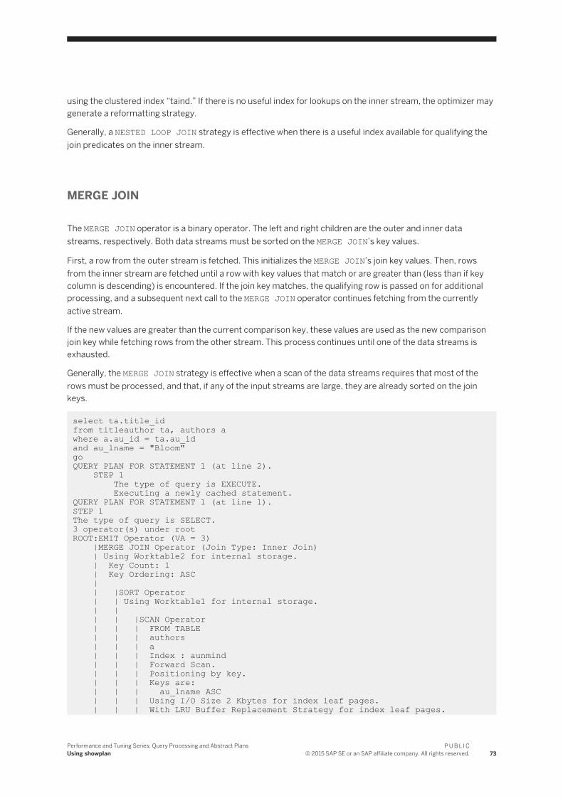
using the clustered index “taind.” If there is no useful index for lookups on the inner stream, the optimizer may generate a reformatting strategy.
Generally, a NESTED LOOP JOIN strategy is effective when there is a useful index available for qualifying the join predicates on the inner stream.
MERGE JOIN
The MERGE JOIN operator is a binary operator. The left and right children are the outer and inner data streams, respectively. Both data streams must be sorted on the MERGE JOIN’s key values.
First, a row from the outer stream is fetched. This initializes the MERGE JOIN’s join key values. Then, rows from the inner stream are fetched until a row with key values that match or are greater than (less than if key column is descending) is encountered. If the join key matches, the qualifying row is passed on for additional processing, and a subsequent next call to the MERGE JOIN operator continues fetching from the currently active stream.
If the new values are greater than the current comparison key, these values are used as the new comparison join key while fetching rows from the other stream. This process continues until one of the data streams is exhausted.
Generally, the MERGE JOIN strategy is effective when a scan of the data streams requires that most of the rows must be processed, and that, if any of the input streams are large, they are already sorted on the join keys.
select ta.title_id from titleauthor ta, authors awhere a.au_id = ta.au_idand au_lname = "Bloom"goQUERY PLAN FOR STATEMENT 1 (at line 2). STEP 1 The type of query is EXECUTE. Executing a newly cached statement.QUERY PLAN FOR STATEMENT 1 (at line 1).STEP 1The type of query is SELECT.3 operator(s) under rootROOT:EMIT Operator (VA = 3) |MERGE JOIN Operator (Join Type: Inner Join) | Using Worktable2 for internal storage. | Key Count: 1 | Key Ordering: ASC | | |SORT Operator | | Using Worktable1 for internal storage. | | | | |SCAN Operator | | | FROM TABLE | | | authors | | | a | | | Index : aunmind | | | Forward Scan. | | | Positioning by key. | | | Keys are: | | | au_lname ASC | | | Using I/O Size 2 Kbytes for index leaf pages. | | | With LRU Buffer Replacement Strategy for index leaf pages.
Performance and Tuning Series: Query Processing and Abstract PlansUsing showplan
P U B L I C© 2015 SAP SE or an SAP affiliate company. All rights reserved. 73

| | | Using I/O Size 2 Kbytes for data pages. | | | With LRU Buffer Replacement Strategy for data pages. | | |SCAN Operator | | FROM TABLE | | titleauthor | | ta | | Index : auidind | | Forward Scan. | | Positioning at index start. | | Using I/O Size 2 Kbytes for index leaf pages. | | With LRU Buffer Replacement Strategy for index leaf pages. | | Using I/O Size 2 Kbytes for data pages. | | With LRU Buffer Replacement Strategy for data pages.
In this example, a sort operator is the left child, or outer stream. The data source for the sort operator is the authors table. The sort operator is required because the authors table has no index on au_id that would otherwise provide the necessary sorted order. A scan of the titleauthor table is the right child/inner stream. The scan uses the auidind index, which provides the necessary ordering for the MERGE JOIN strategy.
A row is fetched from the outer stream (the authors table is the original source) to establish an initial join key comparison value. Then rows are fetched from the titleauthor table until a row with a join key equal to or greater than the comparison key is found.
Inner stream rows with matching keys are stored in a cache in case they need to be refetched. These rows are refetched when the outer stream contains duplicate keys. When a titleauthor.au_id value that is greater than the current join key comparison value is fetched, the MERGE JOIN operator starts fetching from the outer stream until a join key value equal to or greater than the current titleauthor.au_id value is found. The scan of the inner stream resumes at that point.
The MERGE JOIN operator’s showplan output contains a message indicating the worktable to be used for the inner stream’s backing store. The worktable is written to if the inner rows with duplicate join keys no longer fits in cached memory. The width of a cached row is limited to 64 kilobytes.
HASH JOIN Operator
The HASH JOIN operator is a binary operator. The left child generates the build input stream. The right child generates the probe input stream.
The build set is generated by completely draining the build input stream when the first row is requested from the HASH JOIN operator. Every row is read from the input stream and hashed into an appropriate bucket using the hash key.
If there is not enough memory to hold the entire build set, then a portion of it spills to disk. This portion is referred to as a hash partition and should not be confused with table partitions. A hash partition consists of a collection of hash buckets. After the entire left child’s stream has been drained, the probe input is read.
Each row from the probe set is hashed. A lookup is done in the corresponding build bucket to check for rows with matching hash keys. This occurs if the build set’s bucket is memory resident. If it has been spilled, the probe row is written to the corresponding spilled probe partition. When a probe row’s key matches a build row’s key, then the necessary projection of the two row’s columns is passed up for additional processing.
Spilled partitions are processed in subsequent recursive passes of the HASH JOIN algorithm. New hash seeds are used in each pass so that the data is redistributed across different hash buckets. This recursive processing
74P U B L I C© 2015 SAP SE or an SAP affiliate company. All rights reserved.
Performance and Tuning Series: Query Processing and Abstract PlansUsing showplan

continues until the last spilled partition is completely memory resident. When a hash partition from the build set contains many duplicates, the HASH JOIN operator reverts back to NESTED LOOP JOIN processing.
Generally, the HASH JOIN strategy is good in cases where most of the rows from the source sets must be processed and there are no inherent useful orderings on the join keys or there are no interesting orderings that can be promoted to calling operators (for example, an order by clause on the join key). HASH JOINs perform particularly well if one of the data sets is small enough to be memory resident. In this case, no spilling occurs and no I/O is needed to perform that HASH JOIN algorithm.
select ta.title_id from titleauthor ta, authors awhere a.au_id = ta.au_idand au_lname = "Bloom"QUERY PLAN FOR STATEMENT 1 (at line 2).3 operator(s) under rootThe type of query is SELECT.ROOT:EMIT Operator |HASH JOIN Operator (Join Type: Inner Join) | Using Worktable1 for internal storage. | | |SCAN Operator | | FROM TABLE | | authors | | a | | Index : aunmind | | Forward Scan. | | Positioning by key. | | Keys are: | | au_lname ASC | | Using I/O Size 2 Kbytes for index leaf pages. | | With LRU Buffer Replacement Strategy for index leaf pages. | | Using I/O Size 2 Kbytes for data pages. | | With LRU Buffer Replacement Strategy for data pages. | | |SCAN Operator | | FROM TABLE | | titleauthor | | ta | | Index : auidind | | Forward Scan. | | Positioning at index start. | | Using I/O Size 2 Kbytes for index leaf pages. | | With LRU Buffer Replacement Strategy for index leaf pages. | | Using I/O Size 2 Kbytes for data pages. | | With LRU Buffer Replacement Strategy for data pages.
In this example, the source of the build input stream is an index scan of author.aunmind.Only rows with an au_lname value of “Bloom” are returned from this scan. These rows are then hashed on their au_id value and placed into their corresponding hash bucket. After the initial build phase is completed, the probe stream is opened and scanned. Each row from the source index, titleauthor.auidind, is hashed on the au_id column. The resulting hash value is used to determine which bucket in the build set should be searched for matching hash keys. Each row from the build set’s hash bucket is compared to the probe row’s hash key for equality. If the row matches, the titleauthor.au_id column is returned to the EMIT operator.
The HASH JOIN operator’s showplan output contains a message indicating the worktable to be used for the spilled partition’s backing store. The input row width is limited to 64 kilobytes.
Performance and Tuning Series: Query Processing and Abstract PlansUsing showplan
P U B L I C© 2015 SAP SE or an SAP affiliate company. All rights reserved. 75

Hash Join Operator Performance for Parallel Queries
SAP ASE versions 16.0 and later implement performance improvements and a reduction in resource usage for certain parallel query plans involving HASH JOIN operators.
A HASH JOIN operation includes two steps:
1. Building a hash table containing the joining columns of the outer stream of rows to be joined, and2. Probing the hash table with the joining column values of each of the rows in the inner stream to be joined
SAP ASE 16.0 replaces the HASH JOIN operator with the HASH PROBE and the HASH BUILD operators, and includes the replicated EXCHANGE operator between these operators. The HASH BUILD operator builds the hash table and the HASH PROBE operator reads the inner stream and probes the hash table to find matching rows (in earlier releases of SAP ASE, the HASH JOIN operator performed both these steps).
A single worker thread executes the HASH BUILD operator, building a single hash table. The query engine passes this hash table through memory pipes to all producers executing the HASH PROBE operator. These producers share this hash table and probe it for matches to the joining columns in their inner streams. Earlier releases of SAP ASE required multiple producers to execute the HASH JOIN operator.
This is an example of showplan output for a query plan using the HASH JOIN operator:
| | |EXCHANGE Operator (VA = 6) (Merged)| |Executed in parallel by 4 Producer and 1 Consumer processes.| | | | |EXCHANGE:EMIT Operator (VA = 5)| | | | | | |HASH JOIN Operator (VA = 4) (Join Type: Inner Join)| | | | Using Worktable1 for internal storage.| | | | Key Count: 1| | | | | | | | |EXCHANGE Operator (VA = 2) (Replicated)| | | | |Executed in parallel by 1 Producer and 4 Consumer processes.| | | | | | | | | | |EXCHANGE:EMIT Operator (VA = 1) | | | | | |
A query plan must include these attributes for the query processor to use the HASH JOIN improvements:
● The query processor executes the HASH JOIN operator (VA = 4) in parallel (the example above includes four Producers in the EXCHANGE Operator (VA = 6).
● The left child Operator of the HASH JOIN Operator is a Replicated EXCHANGE Operator (VA = 2) with a single Producer
If the query does not meet this criteria, the query processor uses the single HASH JOIN operator.
The benefits of the SAP ASE 16.0 query plan are that it:
● Avoids the performance degradation caused by copying all of the rows through the memory pipes to the producers executing the HASH JOIN operator. Instead, the query engine passes a single row containing a reference to the hash table built by the HASH PROBE operator through the pipes.
● Does not require the extra memory and disk resources needed by each producer to build its own hash table. Instead, it shares a single hash table.
This is an example of showplan output for query plans using the improved hash join processing:
|
76P U B L I C© 2015 SAP SE or an SAP affiliate company. All rights reserved.
Performance and Tuning Series: Query Processing and Abstract PlansUsing showplan

| |EXCHANGE Operator (VA = 7) (Merged)| |Executed in parallel by 4 Producer and 1 Consumer processes.| | | | |EXCHANGE:EMIT Operator (VA = 6)| | | | | | |HASH JOIN PROBE Operator (VA = 5) (Join Type: Inner Join)| | | | Using Worktable2 for internal storage.| | | | Key Count: 1| | | | | | | | |EXCHANGE Operator (VA = 3) (Replicated)| | | | |Executed in parallel by 1 Producer and 4 Consumer processes.| | | | | | | | | | |EXCHANGE:EMIT Operator (VA = 2)| | | | | | | | | | | | |HASH JOIN BUILD Operator (VA = 1) (Join Type: Inner Join)| | | | | | | Using Worktable1 for internal storage.| | | | | | | Key Count: 1| | | | | | |
NARY NESTED LOOP JOIN Operator
The NARY NESTED LOOP JOIN strategy is never evaluated or chosen by the optimizer. It is an operator that is constructed during code generation.
If the compiler finds series of two or more left-deep NESTED LOOP JOINs, it attempts to transform them into a NARY NESTED LOOP JOIN operator. Two additional requirements allow for transformation scan; each NESTED LOOP JOIN operator has an “inner join” type and the right child of each NESTED LOOP JOIN is a SCAN operator. A RESTRICT operator is permitted above the SCAN operator.
NARY NESTED LOOP JOIN execution has a performance benefit over the execution of a series of NESTED LOOP JOIN operators. The example below demonstrates a fundamental difference between the two methods of execution.
With a series of NESTED LOOP JOIN, a scan may eliminate rows based on searchable argument values initialized by an earlier scan. That scan may not be the one that immediately preceded the failing scan. With a series of NESTED LOOP JOINs, the previous scan would be completely drained although it has no effect on the failing scan. This could result in a significant amount of needless I/O. With NARY NESTED LOOP JOINs, the next row fetched comes from the scan that produced the failing searchable argument value, which is far more efficient.
select a.au_id, au_fname, au_lname from titles t, titleauthor ta, authors awhere a.au_id = ta.au_idand ta.title_id = t.title_idand a.au_id = t.title_id and au_lname = "Bloom"
QUERY PLAN FOR STATEMENT 1 (at line 1). STEP 1The type of query is SELECT.4 operator(s) under root |ROOT:EMIT Operator (VA = 4) | | |N-ARY NESTED LOOP JOIN Operator (VA = 3) has 3 children. | | | | | SCAN Operator (VA = 0)
Performance and Tuning Series: Query Processing and Abstract PlansUsing showplan
P U B L I C© 2015 SAP SE or an SAP affiliate company. All rights reserved. 77

| | | FROM TABLE | | | authors | | | a | | | Table Scan. | | | Forward Scan. | | | Positioning at start of table. | | | Using I/O Size 2 Kbytes for data pages. | | | With LRU Buffer Replacement Strategy for data pages. | | | |SCAN Operator (VA = 1) | | | FROM TABLE | | | titleauthor | | | ta | | | Table Scan. | | | Forward Scan. | | | Positioning at start of table. | | | Using I/O Size 2 Kbytes for data pages. | | | With LRU Buffer Replacement Strategy for data pages. | | | | | SCAN Operator (VA = 2) | | | FROM TABLE | | | titles | | | t | | | Index : titles_6720023942 | | | Forward Scan. | | | Positioning by key. | | | Index contains all needed columns. Base table will not be read. | | | Keys are: | | | title_id ASC | | | Using I/O Size 2 Kbytes for index leaf pages. | | | With LRU Buffer Replacement Strategy for index leaf pages.
78P U B L I C© 2015 SAP SE or an SAP affiliate company. All rights reserved.
Performance and Tuning Series: Query Processing and Abstract PlansUsing showplan

All query processor operators are assigned a virtual address. The lines in this figure with VA = report the virtual address for a given operator.
The effective join order is authors, titleauthor, titles. A RESTRICT operator is the parent operator of the scan on titleauthors. This plan is transformed into the NARY NESTED LOOP JOIN plan below:
The transformation retains the original join order of authors, titleauthor, and titles. In this example, the scan of titles has two searchable arguments on it—ta.title_id = t.title_id and a.au_id = t.title_id. So, the scan of titles fails because of the searchable argument value established by the scan of titleauthor, or it fails because of the searchable argument value established by the scan of authors. If no rows are returned from a scan of titles because of the searchable argument value set by the scan of authors, there is no point in continuing the scan of titleauthor. For every row fetched from titleauthor, the scan of titles fails. It is only when a new row is fetched from authors that the scan of titles might succeed. This is why NARY NESTED LOOP JOINs have been implemented; they eliminate the useless draining of tables that have no impact on the rows returned by successive scans.
In the example, the NARY NESTED LOOP JOIN operator closes the scan of titleauthor, fetches a new row from authors, and repositions the scan of titleauthor based on the au_id fetched from authors. Again, this can be a significant performance improvement as it eliminates the needless draining of the titleauthor table and the associated I/O that could occur.
Performance and Tuning Series: Query Processing and Abstract PlansUsing showplan
P U B L I C© 2015 SAP SE or an SAP affiliate company. All rights reserved. 79

Semijoin Operator
The semijoin is a variant of NESTED LOOP JOIN operator, and includes the NESTED LOOP JOIN operator in its result set.
When you make a semi-join between two tables, SAP ASE returns the rows from the first table that contain one or more matches in the second table (a regular join returns the matching rows from the first table only once). That is, instead of scanning a table to return all matching values, an semijoin returns rows when it finds the first matching value and then stops processing. Semijoins are also known as “existence joins.”
For example, if you perform a semijoin on the titles and titleauthor tables:
select title from titleswhere title_id in (select title_id from titleauthor) and title like "A Tutorial%"
QUERY PLAN FOR STATEMENT 1 (at line 1). STEP 1 The type of query is SELECT. 4 operator(s) under root|ROOT:EMIT Operator (VA = 4) | | |NESTED LOOP JOIN Operator (VA = 3) (Join Type: Left Semi Join) | | | | |RESTRICT Operator (VA = 1)(0)(0)(0)(6)(0) | | | | | | |SCAN Operator (VA = 0) | | | | FROM TABLE | | | | titles | | | | Index : titleind | | | | Forward Scan. | | | | Positioning by key. | | | | Keys are: | | | | title ASC | | | | Using I/O Size 2 Kbytes for index leaf pages. | | | | With LRU Buffer Replacement Strategy for index leaf pages. | | | | Using I/O Size 2 Kbytes for data pages. | | | | With LRU Buffer Replacement Strategy for data pages. | | | | |SCAN Operator (VA = 2) | | | FROM TABLE | | | titleauthor | | | Index : titleidind | | | Forward Scan. | | | Positioning by key. | | | Index contains all needed columns. Base table will not be read. | | | Keys are: | | | title_id ASC | | | Using I/O Size 2 Kbytes for index leaf pages. | | | With LRU Buffer Replacement Strategy for index leaf pages.
Distinct Operators
There are three unary operators you can use to enforce distinctness: GROUP SORTED Distinct, SORT Distinct, and HASH Distinct. Each has advantages and disadvantages. The optimizer chooses an efficient distinct operator with respect to its use within the entire query plan’s context.
80P U B L I C© 2015 SAP SE or an SAP affiliate company. All rights reserved.
Performance and Tuning Series: Query Processing and Abstract PlansUsing showplan

GROUP SORTED Distinct Operator
You can use the GROUP SORTED Distinct operator to apply distinctness. GROUP SORTED Distinct requires that the input stream is already sorted on the distinct columns. It reads a row from its child operator and initializes the current distinct columns’ values to be filtered.
The row is returned to the parent operator. When the GROUP SORTED operator is called again to fetch another row, it fetches another row from its child and compares the values to the current cached values. If the value is a duplicate, the row is discarded and the child is called again to fetch a new row.
This process continues until a new distinct row is found. The distinct columns’ values for this row are cached and are used later to eliminate nondistinct rows. The current row is returned to the parent operator for further processing.
The GROUP SORTED Distinct operator returns a sorted stream. The fact that it returns a sorted and distinct data stream are properties that the optimizer can use to improve performance in additional upstream processing. The GROUP SORTED Distinct operator is a nonblocking operator. It returns a distinct row to its parent as soon as it is fetched. It does not require the entire input stream to be processed before it can start returning rows. The following query collects distinct last and first author’s names:
select distinct au_lname, au_fname from authorswhere au_lname = "Bloom"QUERY PLAN FOR STATEMENT 1 (at line 2).STEP 1The type of query is SELECT.2 operator(s) under rootROOT:EMIT Operator (VA = 2) |GROUP SORTED Operator (VA = 1) |Distinct | | |SCAN Operator (VA = 0) | | FROM TABLE | | authors | | Index : aunmind | | Forward Scan. | | Positioning by key. | | Index contains all needed columns. Base table will not be read. | | Keys are: | | au_lname ASC | | Using I/O Size 2 Kbytes for index leaf pages. | | With LRU Buffer Replacement Strategy for index leaf pages.
The GROUP SORTED Distinct operator is chosen in this query plan to apply the distinct property because the scan operator is returning rows in sorted order for the distinct columns au_lname and au_fname. GROUP SORTED incurs no I/O and minimal CPU overhead.
You can use the GROUP SORTED Distinct operator to implement vector aggregation. The showplan output prints the line Distinct to indicate that this GROUP SORTED Distinct operator is implementing the distinct property.
SORT Distinct Operator
The SORT Distinct operator does not require that its input stream is already sorted on the distinct key columns. It is a blocking operator that drains its child operator’s stream and sorts the rows as they are read.
Performance and Tuning Series: Query Processing and Abstract PlansUsing showplan
P U B L I C© 2015 SAP SE or an SAP affiliate company. All rights reserved. 81
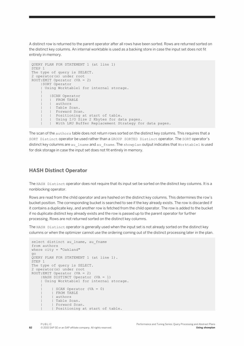
A distinct row is returned to the parent operator after all rows have been sorted. Rows are returned sorted on the distinct key columns. An internal worktable is used as a backing store in case the input set does not fit entirely in memory.
QUERY PLAN FOR STATEMENT 1 (at line 1) STEP 1The type of query is SELECT.2 operator(s) under rootROOT:EMIT Operator (VA = 2) |SORT Operator | Using Worktable1 for internal storage. | | |SCAN Operator | | FROM TABLE | | authors | | Table Scan. | | Forward Scan. | | Positioning at start of table. | | Using I/O Size 2 Kbytes for data pages. | | With LRU Buffer Replacement Strategy for data pages.
The scan of the authors table does not return rows sorted on the distinct key columns. This requires that a SORT Distinct operator be used rather than a GROUP SORTED Distinct operator. The SORT operator’s distinct key columns are au_lname and au_fname. The showplan output indicates that Worktable1 is used for disk storage in case the input set does not fit entirely in memory.
HASH Distinct Operator
The HASH Distinct operator does not require that its input set be sorted on the distinct key columns. It is a nonblocking operator.
Rows are read from the child operator and are hashed on the distinct key columns. This determines the row’s bucket position. The corresponding bucket is searched to see if the key already exists. The row is discarded if it contains a duplicate key, and another row is fetched from the child operator. The row is added to the bucket if no duplicate distinct key already exists and the row is passed up to the parent operator for further processing. Rows are not returned sorted on the distinct key columns.
The HASH Distinct operator is generally used when the input set is not already sorted on the distinct key columns or when the optimizer cannot use the ordering coming out of the distinct processing later in the plan.
select distinct au_lname, au_fname from authors where city = "Oakland"goQUERY PLAN FOR STATEMENT 1 (at line 1).STEP 1The type of query is SELECT.2 operator(s) under rootROOT:EMIT Operator (VA = 2) |HASH DISTINCT Operator (VA = 1) | Using Worktable1 for internal storage. | | | SCAN Operator (VA = 0) | | FROM TABLE | | authors | | Table Scan. | | Forward Scan. | | Positioning at start of table.
82P U B L I C© 2015 SAP SE or an SAP affiliate company. All rights reserved.
Performance and Tuning Series: Query Processing and Abstract PlansUsing showplan

| | Using I/O Size 2 Kbytes for data pages. | | With LRU Buffer Replacement Strategy for data pages.
In this example, the output of the authors table scan is not sorted. The optimizer can choose either a SORT Distinct or HASH Distinct operator strategy. The ordering provided by a SORT Distinct strategy is not useful anywhere else in the plan, so the optimizer will probably choose a HASH Distinct strategy. The optimizer’s decision is ultimately based on cost estimates. The HASH Distinct is typically less expensive for unsorted input streams can eliminate rows on the fly for resident partitions. The SORT Distinct operator cannot eliminate any rows until the entire data set has been sorted.
The showplan output for the HASH Distinct operator reports that Worktable1 will be used. A worktable is needed in case the distinct row result set cannot fit in memory. In that case, partially processed groups are written to disk.
Compute by Message
Processing is done in the EMIT operator, and requires that the EMIT operator’s input stream be sorted according to any order by requirements in the query. The processing is similar to what is done in the GROUP SORTED AGGREGATE operator.
Each row read from the child is checked to see if it starts a new group. If it does not, aggregate functions are applied as appropriate to the query’s requested groups. If a new group is started, the current group and its aggregated values are returned to the user. A new group is then started and its aggregate values are initialized from the new row’s values. This example collects an ordered list of all cities and reports a count of the number of entries for each city after the city list.
select city from authorsorder by citycompute count(city) by cityQUERY PLAN FOR STATEMENT 1 (at line 1).STEP 1The type of query is SELECT.2 operator(s) under rootEmit with Compute semanticsROOT:EMIT Operator (VA = 2) |SORT Operator (VA = 1) | Using Worktable1 for internal storage. | | |SCAN Operator (VA = 0) | | FROM TABLE | | authors | | Table Scan. | | Forward Scan. | | Positioning at start of table. | | Using I/O Size 2 Kbytes for data pages. | | With LRU Buffer Replacement Strategy for data pages.
In this example, the EMIT operator’s input stream is sorted on the city attribute. For each row, the compute by count value is incremented. When a new city value is fetched, the current city’s values and associated count value is returned to the user. The new city value becomes the new compute by grouping value and its count is initialized to one.
Performance and Tuning Series: Query Processing and Abstract PlansUsing showplan
P U B L I C© 2015 SAP SE or an SAP affiliate company. All rights reserved. 83

Related Information
Vector Aggregation Operators [page 84]
2.4.6.1 Vector Aggregation Operators
There are three unary operators used for vector aggregation: the GROUP SORTED COUNT AGGREGATE, the HASH VECTOR AGGREGATE, and the GROUP INSERTING operators.
GROUP SORTED COUNT AGGREGATE Operator
The GROUP SORTED COUNT AGGREGATE operator requires that input set to be sorted on the group by columns. The algorithm is very similar to that of GROUP SORTED Distinct.
A row is read from the child operator. If the row is the start of a new vector, its grouping columns are cached and the aggregation results are initialized.
If the row belongs to the current group being processed, the aggregate functions are applied to the aggregate results. When the child operator returns a row that starts a new group or End Of Scan, the current vector and its aggregated values are returned to the parent operator.
The first row in the GROUP SORTED COUNT AGGREGATE operator is returned after an entire group is processed, where the first row in the GROUP SORTED Distinct operator is returned at the start of a new group. This example collects a list of all cities with the number of authors that live in each city.
select city, total_authors = count(*) from authorsgroup by cityplan"(group_sorted(sort (scan authors)))"QUERY PLAN FOR STATEMENT 1 (at line 1).Optimized using the Abstract Plan in the PLAN clause.STEP 1The type of query is SELECT.3 operator(s) under rootROOT:EMIT Operator (VA = 3) |GROUP SORTED Operator (VA = 2) | Evaluate Grouped COUNT AGGREGATE. | | |SORT Operator (VA = 1) | | Using Worktable1 for internal storage. | | | | | SCAN Operator (VA = 0) | | | FROM TABLE | | | authors | | | Table Scan. | | | Forward Scan. | | | Positioning at start of table. | | | Using I/O Size 2 Kbytes for data pages. | | | With LRU Buffer Replacement Strategy for data pages.
84P U B L I C© 2015 SAP SE or an SAP affiliate company. All rights reserved.
Performance and Tuning Series: Query Processing and Abstract PlansUsing showplan

In this query plan, the scan of authors does not return rows in grouping order. A SORT operator is applied to order the stream based on the grouping column city. At this point, a GROUP SORTED COUNT AGGREGATE operator can be applied to evaluate the count aggregate.
The GROUP SORTED COUNT AGGREGATE operator showplan output reports the aggregate functions being applied as:
| Evaluate Grouped COUNT AGGREGATE.
HASH VECTOR AGGREGATE operator
The HASH VECTOR AGGREGATE operator is a blocking operator.
All rows from the child operator must be processed before the first row from the HASH VECTOR AGGREGATE operator can be returned to its parent operator. Other than this, the algorithm is similar to the HASH Distinct operator’s algorithm.
Rows are fetched from the child operator. Each row is hashed on the query’s grouping columns. The bucket that is hashed is searched to see if the vector already exists.
If the group by values do not exist, the vector is added and the aggregate values are initialized using this first row. If the group by values do exist, the current row is aggregated to the existing values. This example collects a list of all cities with the number of authors that live in each city.
select city, total_authors = count(*) from authorsgroup by cityQUERY PLAN FOR STATEMENT 1 (at line 1).STEP 1The type of query is SELECT.2 operator(s) under rootROOT:EMIT Operator (VA = 2) |HASH VECTOR AGGREGATE Operator (VA = 1) | GROUP BY | Evaluate Grouped COUNT AGGREGATE. | Using Worktable1 for internal storage. | Key Count: 1 | | |SCAN Operator (VA = 0) | | FROM TABLE | | authors | | Table Scan. | | Forward Scan. | | Using I/O Size 2 Kbytes for data pages. | | With LRU Buffer Replacement Strategy for data pages.
In this query plan, the HASH VECTOR AGGREGATE operator reads all of the rows from its child operator, which is scanning the authors table. Each row is checked to see if there is already an entry bucket entry for the current city value. If there is not, a hash entry row is added with the new city grouping value and the count result is initialized to 1. If there is already a hash entry for the new row’s city value, the aggregation function is applied. In this case, the count result is incriminated.
The showplan output prints a group by message specifically for the HASH VECTOR AGGREGATE operator, then prints the grouped aggregation messages:
| Evaluate Grouped COUNT AGGREGATE.
Performance and Tuning Series: Query Processing and Abstract PlansUsing showplan
P U B L I C© 2015 SAP SE or an SAP affiliate company. All rights reserved. 85

The showplan output reports used to store spilled groups and unprocessed rows:
| Using Worktable1 for internal storage.
GROUP INSERTING Operator
GROUP INSERTING is a blocking operator. All rows from the child operator must be processed before the first row can be returned from the GROUP INSERTING.
GROUP INSERTING is limited to 31 or fewer columns in the group by clause. The operator starts by creating a worktable with a clustered index of the grouping columns. As each row is fetched from the child, a lookup into the work table is done based on the grouping columns. If no row is found, then the row is inserted. This effectively creates a new group and initializes its aggregate values. If a row is found, the new aggregate values are updated based on evaluating the new values. The GROUP INSERTING operator returns rows ordered by the grouping columns.
select city, total_authors = count(*) from authorsgroup by cityplan '(group_inserting (i_scan auidind authors ))'
QUERY PLAN FOR STATEMENT 1 (at line 1). Optimized using the Abstract Plan in the PLAN clause.STEP 1The type of query is SELECT.2 operator(s) under root |ROOT:EMIT Operator (VA = 2)|| |GROUP INSERTING Operator (VA = 1)| | GROUP BY| | Evaluate Grouped COUNT AGGREGATE| | Using Worktable1 for internal storage.| || | |SCAN Operator (VA = 0)| | | FROM TABLE| | | authors| | | Table Scan.| | | Forward Scan.| | | Positioning at start of table.| | | Using I/O Size 2 Kbytes for data pages. | | | With LRU Buffer Replacement Strategy for data pages.
In this example, the group inserting operator starts by building a worktable with a clustered index keyed on the city column. The group inserting operator proceeds to drain the authors table. For each row, a lookup is done on the city value. If there is no row in the aggregation worktable with the current city value, then the row is inserted. This creates a new group for the current city value with an initialized count value. If the row for the current city value is found, then an evaluation is done to increment the COUNT AGGREGATE value.
86P U B L I C© 2015 SAP SE or an SAP affiliate company. All rights reserved.
Performance and Tuning Series: Query Processing and Abstract PlansUsing showplan

2.5 Union Operators
SAP ASE UNION operators include the UNION ALL, MERGE UNION, and HASH UNION operators.
2.5.1 UNION ALL Operator
The UNION ALL operator merges several compatible input streams without performing any duplicate elimination. Every data row that enters the UNION ALL operator is included in the operator’s output stream.
The UNION ALL operator is a nary operator that displays this message:
UNION ALL OPERATOR has <N> children.
<N> is the number of input streams into the operator.
This example demonstrates the use of UNION ALL:
select * from sysindexes where id < 100 union all select * from sysindexes where id > 200
QUERY PLAN FOR STATEMENT 1 (at line 1).
STEP 1 The type of query is SELECT.3 operator(s) under root |ROOT:EMIT Operator (VA = 3) | | |UNION ALL Operator (VA = 2) has 2 children. | |
| | |SCAN Operator (VA = 0) | | | FROM TABLE | | | sysindexes | | | Using Clustered Index. | | | Index : csysindexes | | | Forward Scan. | | | Positioning by key. | | | Keys are: | | | id ASC | | | Using I/O Size 2 Kbytes for index leaf pages. | | | With LRU Buffer Replacement Strategy for index leaf pages. | | | Using I/O Size 2 Kbytes for data pages. | | | With LRU Buffer Replacement Strategy for data pages. | | | | |SCAN Operator (VA = 1) | | | FROM TABLE | | | sysindexes | | | Using Clustered Index | | | Index : csysindexes | | | Forward scan. | | | Positioning by key. | | | Keys are: | | | id ASC | | | Using I/O Size 2 Kbytes for index leaf pages. | | | With LRU Buffer Replacement Strategy for index leaf pages.
Performance and Tuning Series: Query Processing and Abstract PlansUsing showplan
P U B L I C© 2015 SAP SE or an SAP affiliate company. All rights reserved. 87
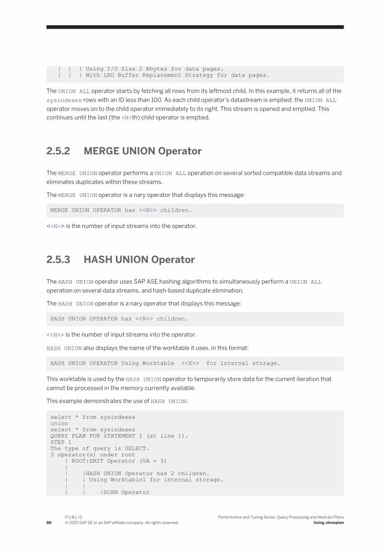
| | | Using I/O Size 2 Kbytes for data pages. | | | With LRU Buffer Replacement Strategy for data pages.
The UNION ALL operator starts by fetching all rows from its leftmost child. In this example, it returns all of the sysindexes rows with an ID less than 100. As each child operator’s datastream is emptied, the UNION ALL operator moves on to the child operator immediately to its right. This stream is opened and emptied. This continues until the last (the <N>th) child operator is emptied.
2.5.2 MERGE UNION Operator
The MERGE UNION operator performs a UNION ALL operation on several sorted compatible data streams and eliminates duplicates within these streams.
The MERGE UNION operator is a nary operator that displays this message:
MERGE UNION OPERATOR has <<N>> children.
<<N>> is the number of input streams into the operator.
2.5.3 HASH UNION Operator
The HASH UNION operator uses SAP ASE hashing algorithms to simultaneously perform a UNION ALL operation on several data streams, and hash-based duplicate elimination.
The HASH UNION operator is a nary operator that displays this message:
HASH UNION OPERATOR has <<N>> children.
<<N>> is the number of input streams into the operator.
HASH UNION also displays the name of the worktable it uses, in this format:
HASH UNION OPERATOR Using Worktable <<X>> for internal storage.
This worktable is used by the HASH UNION operator to temporarily store data for the current iteration that cannot be processed in the memory currently available.
This example demonstrates the use of HASH UNION:
select * from sysindexes unionselect * from sysindexesQUERY PLAN FOR STATEMENT 1 (at line 1).STEP 1The type of query is SELECT.3 operator(s) under root | ROOT:EMIT Operator (VA = 3) | | |HASH UNION Operator has 2 children. | | Using Worktable1 for internal storage. | | | | |SCAN Operator
88P U B L I C© 2015 SAP SE or an SAP affiliate company. All rights reserved.
Performance and Tuning Series: Query Processing and Abstract PlansUsing showplan

| | | FROM TABLE | | | sysindexes | | | Table Scan. | | | Forward Scan. | | | Positioning at start of table. | | | Using I/O Size 2 Kbytes for data pages. | | | With LRU Buffer Replacement Strategy for data pages. | | | |SCAN Operator (VA = 1) | | | FROM TABLE | | | sysindexes | | | Table Scan. | | | Forward Scan. | | | Positioning at start of table. | | | Using I/O size 2 Kbytes for data pages. | | | With LRU Buffer Replacement Strategy for data pages.
2.5.4 SCALAR AGGREGATE Operator
The SCALAR AGGREGATE operator keeps track of running information about an input data stream, such as the number of rows in the stream, or the maximum value of a given column in the stream.
The SCALAR AGGREGATE operator prints a list of up to 10 messages describing the scalar aggregation operations it executes. The message has the following format:
Evaluate Ungrouped <Type of Aggregate> Aggregate
<Type of Aggregate> can be any of the following: count, sum, average, min, max, any, once-unique, count-unique, sum-unique, average-unique, or once.
The following query performs a SCALAR AGGREGATE (that is, unwrapped) aggregation on the authors table in the pubs2 database:
select count(*) from authors QUERY PLAN FOR STATEMENT 1 (at line 1).STEP 1The type of query is SELECT.2 operator(s) under rootROOT:EMIT Operator (VA = 2) |SCALAR AGGREGATE Operator (VA = 1) | Evaluate Ungrouped COUNT AGGREGATE. | | |SCAN Operator (VA =0) | | FROM TABLE | | authors | | Index : aunmind | | Forward Scan. | | Positioning at index start. | | Index contains all needed columns. Base table will not be read. | | Using I/O Size 4 Kbytes for index leaf pages. | | With LRU Buffer Replacement Strategy for index leaf pages.
The SCALAR AGGREGATE message indicates that the query to be executed is an ungrouped count aggregation.
Performance and Tuning Series: Query Processing and Abstract PlansUsing showplan
P U B L I C© 2015 SAP SE or an SAP affiliate company. All rights reserved. 89

2.5.5 RESTRICT Operator
The RESTRICT operator is a unary operator that evaluates expressions based on column values.
The RESTRICT operator is associated with multiple column evaluations lists that can be processed before fetching a row from the child operator, after fetching a row from the child operator, or to compute the value of virtual columns after fetching a row from the child operator.
2.5.6 SORT Operator
The SORT operator has only one child operator within the query plan. Its role is to generate an output data stream from the input stream, using a specified sorting key.
The SORT operator may execute a streaming sort when possible, but may also have to store results temporarily into a worktable. The SORT operator displays the worktable’s name in this format:
Using Worktable<N> for internal storage.
where <<N>> is a numeric identifier for the worktable within the showplan output.
Here is an example of a simple query plan using a SORT operator and a worktable:
select au_id from authors order by postalcode QUERY PLAN FOR STATEMENT 1 (at line 1).STEP 1The type of query is SELECT.2 operator(s) under rootROOT:EMIT Operator (VA = 2) |SORT Operator (VA = 1) | Using Worktable1 for internal storage. | | |SCAN Operator (VA = 0) | | FROM TABLE | | authors | | Table Scan. | | Forward Scan. | | Positioning at start of table. | | Using I/O Size 4 Kbytes for data pages. | | With LRU Buffer Replacement Strategy for data pages.
The SORT operator drains its child operator and sorts the rows. In this case, it sorts each row fetched from the authors table using the postalcode attribute. If all of the rows fit into memory, then no data is spilled to disk. But, if the input data’s size exceeds the available buffer space, then sorted runs are spilled to disk. These runs are recursively merged into larger sorted runs until there are fewer runs than there are available buffers to read and merge the runs with.
2.5.6.1 SORT Operator Performance for Parallel Queries
SAP ASE version 16.0 and later improves the performance on certain parallel queries that include SORT operators.
To benefit from the changes, the parallel query must include:
90P U B L I C© 2015 SAP SE or an SAP affiliate company. All rights reserved.
Performance and Tuning Series: Query Processing and Abstract PlansUsing showplan

● A SORT operator that appears on top of the Exchange operator● Exchange operator must be a Replicated Exchange with a single producer and multiple consumers.
If the query does not meet this criteria, the query processor uses the standard SORT operator included with SAP ASE versions earlier than 16.0 (also called the DEFAULT sort).
This example is from a version of SAP ASE earlier than 16.0, and does not include the SORT operator changes:
| | | | |MERGE JOIN Operator (Join Type: Inner Join) (VA = 5) | | | | | Using Worktable2 for internal storage.| | | | | Key Count: 1| | | | | Key Ordering: ASC| | | | || | | | | |SORT Operator (VA = 3)| | | | | | Using Worktable1 for internal storage.| | | | | || | | | | | |EXCHANGE Operator (VA = 2) (Replicated)| | | | | | |Executed in parallel by 1 Producer and 8 Consumer processes.| | | | | | || | | | | | | |EXCHANGE:EMIT Operator (VA = 1)| | | | | | | || | | | | | | | |SCAN Operator (VA = 0)| | | | | | | | | FROM TABLE| | | | | | | | | t2| | | | | | | | | Table Scan.| | | | | | | | | Forward Scan.| | | | | | | | | Positioning at start of table.| | | | | | | | | Using I/O Size 16 Kbytes for data pages.| | | | | | | | | With LRU Buffer Replacement Strategy for data pages.
However, SAP ASE version 16.0 and later moves the build part of the SORT operator below the Exchange Operator and keeps the sort-table reading part above the Exchange, which results in this query execution plan for the same query
| | | | |MERGE JOIN Operator (Join Type: Inner Join) (VA = 6) | | | | | Using Worktable3 for internal storage.| | | | | Key Count: 1| | | | | Key Ordering: ASC| | | | || | | | | |SORT (GETSORTED) Operator (VA = 4)| | | | | | Using Worktable2 for internal storage.| | | | | || | | | | | |EXCHANGE Operator (VA = 3) (Replicated)| | | | | | |Executed in parallel by 1 Producer and 8 Consumer processes.| | | | | | || | | | | | | |EXCHANGE:EMIT Operator (VA = 2)| | | | | | | || | | | | | | | |SORT (SORTBUILD) Operator (VA = 1)| | | | | | | | | Using Worktable1 for internal storage.| | | | | | | | || | | | | | | | | |SCAN Operator (VA = 0)| | | | | | | | | | FROM TABLE| | | | | | | | | | t2| | | | | | | | | | Table Scan.| | | | | | | | | | Forward Scan.| | | | | | | | | | Positioning at start of table.| | | | | | | | | | Using I/O Size 16 Kbytes for data pages. | | | | | | | | | | With LRU Buffer Replacement Strategy for data pages.
The benefits of the new parallel SORT operator are that it:
Performance and Tuning Series: Query Processing and Abstract PlansUsing showplan
P U B L I C© 2015 SAP SE or an SAP affiliate company. All rights reserved. 91

● Splits the SORT operator into two operators: SORTBUILD and GETSORTED. A single sort table built by the SORTBUILD is used by multiple instances of GETSORTED for a parallel reading of sorted rows, reducing the I/Os. The DEFAULT SORT operator plan creates multiple copies of SortTables (8 Consumer processes in the first example).
● Sends a single row containing meta data from the SORTBUILD operator to multiple instances of GETSORTED operator, providing a reference for accessing the sort-table directly, which avoids copying and propagating many rows via Exchange.
The parallel SORT operator includes these restrictions:
● Does not support Repartitioned Exchange. However, SORT operators that occur above Repartitioned Exchange use the DEFAULT sort in the query execution plan.
● Although abstract plans do not explicitly support forcing GETSORTED and SORTBUILD, you can force these plans by making sure the SORT operator appears above the Replicated Exchange.
● SAP ASE implicitly disables dynamic thread assignment (DTA) for the query execution plan that contains GETSORTED and SORTBUILD operators.
2.5.7 STORE Operator
The STORE operator creates a worktable, fills it, and possibly creates an index on it.
As part of the execution of a query plan, the worktable is used by other operators in the plan. A SEQUENCER operator guarantees that the plan fragment corresponding to the worktable and potential index creation is executed before other plan fragments that use the worktable. This is important when a plan is executed in parallel, because execution processes operate asynchronously.
Reformatting strategies use the STORE operator to create a worktable with a clustered index on it.
If the STORE operator is used for a reformatting operation, it prints this message:
Worktable <X> created, in <L> locking mode for reformatting.
The locking mode <L> has to be one of “allpages,” “datapages,” or “datarows.”
The STORE operator also prints this message:
Creating clustered index.
If the STORE operator is not used for a reformatting operation, it prints this message:
Worktable <X> created, in <L> locking mode.
The following example applies to the STORE operator, as well as to the SEQUENCER operator.
select * from bigun a, bigun b where a.c4 = b.c4 and a.c2 < 10
QUERY PLAN FOR STATEMENT 1 (at line 1). Optimized using the Abstract Plan in the PLAN clause.STEP 1 The type of query is SELECT. 7 operator(s) under root |ROOT:EMIT Operator (VA = 7)
92P U B L I C© 2015 SAP SE or an SAP affiliate company. All rights reserved.
Performance and Tuning Series: Query Processing and Abstract PlansUsing showplan

| | |SEQUENCER Operator (VA = 6) has 2 children. | | | | |STORE Operator (VA = 5) | | | Worktable1 created, in allpages locking mode, for REFORMATTING. | | | Creating clustered index. | | | | | | |INSERT Operator(VA = 4) | | | | The update mode is direct. | | | | | | | | |SCAN Operator(VA = 0) | | | | | FROM TABLE | | | | | bigun | | | | | b | | | | | Table Scan. | | | | | Forward Scan. | | | | | Positioning at start of table. | | | | | Using I/O Size 2 Kbytes for data pages. | | | | | With LRU Buffer Replacement Strategy for data pages. | | | | | | | | TO TABLE (VA = 3) | | | | Worktable1. | | | | |NESTED LOOP JOIN (Join Type: Inner Join)(VA = 7) | | | | | | |SCAN Operator (VA = 2) | | | | FROM TABLE | | | | bigun | | | | a | | | | Table Scan. | | | | Forward Scan. | | | | Positioning at start of table. | | | | Using I/O Size 2 Kbytes for data pages. | | | | With LRU Buffer Replacement Strategy for data pages. | | | | | | |SCAN Operator (VA = 1) | | | | FROM TABLE | | | | Worktable1. | | | | Using Clustered Index. | | | | Forward Scan. | | | | Positioning key. | | | | Using I/O Size 2 Kbytes for data pages. | | | | With LRU Buffer Replacement Strategy for data pages.
In the example plan shown above, the STORE operator is used in a reformatting strategy. It is located directly below the SEQUENCER operator in the leftmost child of the SEQUENCER operator.
The STORE operator creates Worktable1, which is filled by the INSERT operator below it. The STORE operator then creates a clustered index on Worktable1. The index is built on the join key b.c4.
2.5.8 SEQUENCER Operator
The SEQUENCER operator is a nary operator that sequentially executes each child plan below it. It also used in reformatting plans, and certain aggregate processing plans.
The SEQUENCER operator executes each of its child subplans, except for the rightmost one. Once all the left child subplans are executed, the rightmost subplan is executed.
Performance and Tuning Series: Query Processing and Abstract PlansUsing showplan
P U B L I C© 2015 SAP SE or an SAP affiliate company. All rights reserved. 93

The SEQUENCER operator displays this message:
SEQUENCER operator has <N> children.
select * from tab1 a, tab2 b where a.c4 = b.c4 and a.c2 < 10
QUERY PLAN FOR STATEMENT 1 (at line 1). Optimized using the Abstract Plan in the PLAN clause. STEP 1 The type of query is SELECT. 7 operator(s) under root |ROOT:EMIT Operator (VA = 7) | | |SEQUENCER Operator (VA = 6) has 2 children. | | | | |STORE Operator (VA = 5) | | | Worktable1 created, in allpages locking mode, for REFORMATTING. | | | Creating clustered index. | | | | | | |INSERT Operator (VA = 4) | | | | The update mode is direct. | | | | | | | | |SCAN Operator (VA = 0) | | | | | FROM TABLE | | | | | tab2 | | | | | b | | | | | Table Scan. | | | | | Forward Scan. | | | | | Positioning at start of table. | | | | | Using I/O Size 2 Kbytes for data pages. | | | | | With LRU Buffer Replacement Strategy for data pages. | | | | | | | | TO TABLE | | | | Worktable1. | | | | |NESTED LOOP JOIN Operator (Join Type: Inner Join) (VA = 3) | | | | | | |SCAN Operator (VA = 2) | | | | FROM TABLE | | | | tab1 | | | | a | | | | Table Scan. | | | | Forward Scan. | | | | Positioning at start of table. | | | | Using I/O Size 2 Kbytes for data pages. | | | | With LRU Buffer Replacement Strategy for data pages. | | | | | | |SCAN Operator (VA = 1) | | | | FROM TABLE | | | | Worktable1. | | | | Using Clustered Index. | | | | Forward Scan. | | | | Positioning by key. | | | | Using I/O Size 2 Kbytes for data pages. | | | | With LRU Buffer Replacement Strategy for data pages.
In this example, the SEQUENCER operator implements a reformatting strategy. The leftmost branch of the SEQUENCER operator creates a clustered index on Worktable1. This branch is executed and closed before the SEQUENCER operator proceeds to the next child operator. The SEQUENCER operator arrives at the rightmost child, opens, and begins to drain it, returning rows back to its parent operator. The design intent of the SEQUENCER operator is for operators in the rightmost branch to use the worktables created in the preceding outer branches of the SEQUENCER operator. In this example, Worktable1 is used in a nested-loop join
94P U B L I C© 2015 SAP SE or an SAP affiliate company. All rights reserved.
Performance and Tuning Series: Query Processing and Abstract PlansUsing showplan

strategy. The scan of Worktable1 is positioned by a key on its clustered index for each row that comes from the outer scan of tab1.
2.5.9 REMOTE SCAN Operator
The REMOTE SCAN operator sends a SQL query to a remote server for execution. It then processes the results returned by the remote server, if any. REMOTE SCAN displays the formatted text of the SQL query it handles.
REMOTE SCAN has 0 or 1 child operators.
2.5.10 SCROLL Operator
The SCROLL operator encapsulates the functionality of scrollable cursors.
Scrollable cursors may be insensitive, meaning that they display a snapshot of their associated data, taken when the cursor is opened, or semi-sensitive, meaning that the next rows to be fetched are retrieved from the live data.
The SCROLL operator is a unary operator that displays this message:
SCROLL OPERATOR ( Sensitive Type: <T>)
The type may be insensitive or semi-sensitive.
This is an example of a plan featuring an insensitive scrollable cursor:
declare CI insensitive scroll cursor for select au_lname, au_id from authorsgoset showplan ongoopen CIQUERY PLAN FOR STATEMENT 1 (at line 1).STEP 1The type of query is OPEN CURSOR CI.QUERY PLAN FOR STATEMENT 1 (at line 2).STEP 1The type of query is DECLARE CURSOR.2 operator(s) under rootROOT:EMIT Operator (VA = 2) |SCROLL Operator (Sensitive Type: Insensitive) (VA = 1) | Using Worktable1 for internal storage. | | |SCAN Operator (VA = 0) | | FROM TABLE | | authors | | Table Scan. | | Forward Scan. | | Positioning at start of table. | | Using I/O Size 4 Kbytes for data pages. | | With LRU Buffer Replacement Strategy for data pages.
The SCROLL operator is the child operator of the root EMIT operator, and its only child is the SCAN operator on the authors table. SCROLL message specifies that the CI cursor is insensitive.
Performance and Tuning Series: Query Processing and Abstract PlansUsing showplan
P U B L I C© 2015 SAP SE or an SAP affiliate company. All rights reserved. 95

Scrollable cursor rows are initially cached in memory. Worktable1 is used as a backing store for this cache when the amount of data processed exceeds the cache’s physical memory limits.
2.5.11 RID JOIN Operator
The RID JOIN operator is a binary operator that joins two data streams, based on row IDs that are generated for the same source table.
Each data row in a SQL table is associated with a unique row ID (RID). Think of a rid-join as a special case of a self-join query. The left child fills a worktable with the set of uniquely qualifying RIDs. The RIDs are the result of applying a distinct filter to the RIDs returned from two or more disparate index cases of the same source table.
The RID JOIN operator is used to implement the general or strategy. The general-or strategy is often used when a query’s predicate contains a collection of disjunctions that can be qualified by different indexes on the same table. In this case, each index is scanned based on the predicates that can be qualified by that index. For each index row that qualifies, a RID is returned.
The returned RIDs are processed for uniqueness so that the same row is not returned twice, which might happen if two or more of the disjunctions qualify the same row.
The RID JOIN operator inserts the unique RIDs into a worktable. The worktable of unique RIDs is passed to the scan operator in the rid-join’s right branch. The access methods can iteratively fetch the next RID to be processed directly from the worktable, and look up the associated row. This row is then returned to the RID JOIN parent operator.
The RID JOIN operator displays this message:
Using Worktable <N> for internal storage.
This worktable is used to store the unique RIDs generated from the left child.
The following example demonstrates the showplan output for the RID JOIN operator.
select * from tab1 a where a.c1 = 10 or a.c3 = 10 QUERY PLAN FOR STATEMENT 1 (at line 2). STEP 1The type of query is SELECT.6 operator(s) under root. |ROOT:EMIT Operator (VA = 6) | | |RID JOIN Operator (VA = 5) | | Using Worktable2 for internal storage. | | | | |HASH UNION Operator (VA = 6) has 2 children. | | | Key Count: 1 | | | | | | |SCAN Operator (VA = 0) | | | | FROM TABLE | | | | tab1 | | | | a | | | | Index:tab1idx | | | | Forward Scan. | | | | Positioning by key. | | | | Index contains all needed columns. Base table will not be read. | | | | Keys are: | | | | c1 ASC | | | | Using I/O Size 2 Kbytes for index leaf pages.
96P U B L I C© 2015 SAP SE or an SAP affiliate company. All rights reserved.
Performance and Tuning Series: Query Processing and Abstract PlansUsing showplan

| | | | With LRU Buffer Replacement Strategy for index leaf pages. | | | | | | |SCAN Operator (VA = 4) | | | | FROM TABLE | | | | tab1 | | | | a | | | | Index:tab1idx2 | | | | Forward Scan. | | | | Positioning by key. | | | | Index contains all needed columns. Base table will not be read. | | | | Keys are: | | | | c3 ASC | | | | Using I/O Size 2 Kbytes for index leaf pages. | | | | With LRU Buffer Replacement Strategy for index leaf pages. | | | | |RESTRICT Operator (VA = 3) | | | | | | |SCAN Operator (VA = 2) | | | | FROM TABLE | | | | tab1 | | | | a | | | | Using Dynamic Index. | | | | Forward Scan. | | | | Positioning by Row IDentifier (RID). | | | | Using I/O Size 2 Kbytes for data pages. | | | | With LRU Buffer Replacement Strategy for data pages.
In this example, the index tab1idx is scanned to get all RIDs from tab1 that have a c1 value of 10. SAP ASE scans tab1idx2 to get all RIDs from tab1 that have a c3 value of 10.
The HASH UNION operator is used to eliminate duplicate RIDs. There are duplicate RIDs for any tab1 rows where both c1 and c3 rows have a value of 10.
The RID JOIN operator inserts all of the returned rows into Worktable2. Worktable2 is passed to the scan of tab1 after it has been completely filled. The access methods fetch the first RID, look up the associated row, and return it to the RID JOIN operator. On subsequent calls to the tab1’s scan operator, the access methods fetch the next RID to be processed and return its associated row.
2.5.12 SQLFILTER Operator
The SQLFILTER operator is a nary operator that executes subqueries. Its leftmost child represents the outer query, and the other children represent query plan fragments that are associated with one or more subqueries.
The leftmost child generates correlation values that are substituted into the other child plans.
The SQLFILTER operator displays this message:
SQFILTER Operator has <N> children.
This example illustrates the use of SQLFILTER:
select pub_name from publishers where pub_id =(select distinct titles.pub_id from titles where publishers.pub_id = titles.pub_id and price > $1000)
Performance and Tuning Series: Query Processing and Abstract PlansUsing showplan
P U B L I C© 2015 SAP SE or an SAP affiliate company. All rights reserved. 97

QUERY PLAN FOR STATEMENT 1 (at line 1). 4 operator(s) under rootSTEP 1The type of query is SELECT.4 operator(s) under rootROOT:EMIT Operator (VA = 4) |SQFILTER Operator (VA = 3) has 2 children. | | |SCAN Operator (VA = 0) | | FROM TABLE | | publishers | | Table Scan. | | Forward Scan. | | Positioning at start of table. | | Using I/O Size 8 Kbytes for data pages. | | With LRU Buffer Replacement Strategy for data pages. | | Run subquery 1 (at nesting level 1) | | QUERY PLAN FOR SUBQUERY 1 (at nesting level 1 and at line 3) | | Correlated Subquery | Subquery under an EXPRESSION predicate. | | |SCALAR AGGREGATE Operator (VA = 2) | | Evaluate Ungrouped ONCE-UNIQUE AGGREGATE | | | | |SCAN Operator (VA = 1) | | | FROM TABLE | | | titles | | | Table Scan. | | | Forward Scan. | | | Postitioning at start of table. | | | Using I/O Size 8 Kbytes for data pages. | | | With LRU Buffer Replacement Strategy for data pages. | | END OF QUERY PLAN FOR SUBQUERY 1
The SQLFILTER operator has two children in this example. The leftmost child is the query’s outer block. It is a simple scan of the publishers table. The right child is used to evaluate the query’s subquery. SQLFILTER fetch rows from the outer block. For every row from the outer block, SQLFILTER invokes the right child to evaluate the subquery. If the subquery evaluates to TRUE, a row is returned to the SQLFILTER’s parent operator.
2.5.13 EXCHANGE Operator
The EXCHANGE operator is a unary operator that encapsulates parallel processing of queries.
EXCHANGE can be located almost anywhere in a query plan and divides the query plan into plan fragments. A plan fragment is a query plan tree that is rooted at an EMIT or EXCHANGE:EMIT operator and has leaves that are SCAN or EXCHANGE operators. A serial plan is a plan fragment that is executed by a single process.
An EXCHANGE operator’s child operator is always an EXCHANGE:EMIT operator. EXCHANGE:EMIT is the root of a new plan fragment. An EXCHANGE operator has an associated server process called the Beta process that acts as a local execution coordinator for the EXCHANGE operator’s worker processes. Worker processes execute the plan fragment as directed by the parent EXCHANGE operator and its Beta process. The plan fragment is often executed in a parallel fashion, using two or more processes. The EXCHANGE operator and Beta process coordinate activities, including the exchange of data between the fragment boundaries.
98P U B L I C© 2015 SAP SE or an SAP affiliate company. All rights reserved.
Performance and Tuning Series: Query Processing and Abstract PlansUsing showplan

The topmost plan fragment, rooted at an EMIT operator rather than an EXCHANGE:EMIT operator, is executed by the Alpha process. The Alpha process is a consumer process associated with the user connection. The Alpha process is the global coordinator of all of the query plan’s worker processes. It is responsible for initially setting up all of the plan fragment’s worker processes and eventually freeing them. It manages and coordinates all of the fragment’s worker processes in the case of an exception.
The EXCHANGE operator displays this message:
Executed in parallel by <N> producer and <P> consumer processes.
The number of producers refers to the number of worker processes that execute the plan fragment located beneath the EXCHANGE operator. The number of consumers refers to the number of worker processes that execute the plan fragment that contains the EXCHANGE operator. The consumers process the data passed to them by the producers. Data is exchanged between the producer and consumer processes through a pipe set up in the EXCHANGE operator. The producer’s EXCHANGE:EMIT operator writes rows into the pipe while consumers read rows from this pipe. The pipe mechanism synchronizes producer writes and consumer reads such that no data is lost.
This example illustrates a parallel query in the master database against the system table sysmessages:
use master goset showplan ongoselect count(*) from sysmessages t1 plan '(t_scan t1) (prop t1 (parallel 4))QUERY PLAN FOR STATEMENT 1 (at line 1).Optimized using the forced options (internally generated Abstract Plan).Executed in parallel by coordinating process and 4 worker processes.4 operator(s) under rootThe type of query is SELECT.ROOT:EMIT Operator |SCALAR AGGREGATE Operator | Evaluate Ungrouped COUNT AGGREGATE. | | |EXCHANGE Operator | |Executed in parallel by 4 Producer and 1 Consumer processes. | | | | |EXCHANGE:EMIT Operator | | | | | | |SCAN Operator | | | | FROM TABLE | | | | sysmessages | | | | Table Scan. | | | | Forward Scan. | | | | Positioning at start of table. | | | | Executed in parallel with a 4-way hash scan. | | | | Using I/O Size 4 Kbytes for data pages. | | | | With LRU Buffer Replacement Strategy for data pages.
There are two plan fragments in this example. The first fragment in any plan, parallel or not, is always rooted by an EMIT operator. The first fragment in this example consists of the EMIT, SCALAR AGGREGATE, and EXCHANGE operators. This first fragment is always executed by the single Alpha process. In this example, it also acts as the Beta process responsible for managing the EXCHANGE operator’s worker processes.
Performance and Tuning Series: Query Processing and Abstract PlansUsing showplan
P U B L I C© 2015 SAP SE or an SAP affiliate company. All rights reserved. 99

The second plan fragment is rooted at the EXCHANGE:EMIT operator. Its only child operator is the SCAN operator. The SCAN operator is responsible for scanning the sysmessages table. The scan is executed in parallel:
Executed in parallel with a 4-way hash scan
This indicates that each worker process is responsible for approximately a quarter of the table. Pages are assigned to the worker processes based on having the data page ID.
The EXCHANGE:EMIT operator writes data rows to the consumers by writing to a pipe created by its parent EXCHANGE operator. In this example, the pipe is a four-to-one demultiplexer, and include several pipe types that perform quite different behaviors.
2.6 INSTEAD-OF TRIGGER Operators
The operators associated with the instead-of triggers feature are INSTEAD-OF TRIGGER and CURSOR SCAN.
The instead-of trigger feature is available as of SAP ASE version 15.0.2. The instead-of trigger feature uses pseudotables, which allow the user to apply specific actions for inserts, deletes, and updates on views, when these actions would otherwise have been ambiguous.
2.6.1 INSTEAD-OF TRIGGER Operator
The INSTEAD-OF TRIGGER operator appears only in query plans for insert, update, or delete statements on a view that has an instead-of trigger created upon it.
Its function is to create and fill the inserted and deleted pseudotables that are used in the trigger to examine the rows that would have been modified by the original insert, update, or delete query. The only purpose of the query plan that contains an INSTEAD-OF TRIGGER operator is to fill the inserted and deleted tables—the actual operation of the original SQL statement is never attempted on the view referenced in the statement. Rather, it is up to the trigger to perform the updates to the view’s underlying tables based on the data available in the inserted and deleted pseudo tables.
The following is an example of the INSTEAD-OF TRIGGER operator’s showplan output:
create table t12 (c0 int primary key, c1 int null, c2 int null) go. . .create view t12view as select c1,c2 from t12gocreate trigger v12updtrg on t12viewinstead of update asselect * from deletedgoupdate t12view set c1 = 3QUERY PLAN FOR STATEMENT 1 (at line 1). STEP 1 The type of query is SELECT.2 operator(s) under root |ROOT:EMIT Operator (VA = 1)
100P U B L I C© 2015 SAP SE or an SAP affiliate company. All rights reserved.
Performance and Tuning Series: Query Processing and Abstract PlansUsing showplan

| | |INSTEAD-OF TRIGGER Operator | | Using Worktable1 for internal storage. | | Using Worktable2 for internal storage. | | | | |SCAN Operator (VA = 0) | | | FROM TABLE | | | t12 | | | Table Scan. | | | Forward Scan. | | | Positioning at start of table. | | | Using I/O Size 2 Kbytes for data pages. | | | With LRU Buffer Replacement Strategy for data pages.
In this example, the v12updtrig instead-of trigger is defined on the t12view. The update to the t12view results in the creation of the INSTEAD-OF TRIGGER operator. The INSTEAD-OF TRIGGER operator creates two worktables. Worktable1 and Worktable2 are used to hold the inserted and deleted rows, respectively. These worktables are unique in that they persist across statements. Trigger execution results in the following showplan lines getting printed.
QUERY PLAN FOR STATEMENT 1 (at line 3). STEP 1 The type of query is SELECT.1 operator(s) under root |ROOT:EMIT Operator (VA = 1) | | |SCAN Operator (VA = 0) | | FROM CACHE
The showplan statement output above is for the trigger’s statement, select * from deleted. The rows to be deleted from the view were inserted into the “deleted” cache when the initial update statement was executed. Then, the trigger scans the table to report what rows would have been deleted from the t12view view.
2.6.2 CURSOR SCAN Operator
The CURSOR SCAN operator only appears in positioned delete or update (that is, delete <view-name> where current of <cursor_name> ) statements on a view that has an instead-of trigger created upon it. As such, it appears only as a child operator of the INSTEAD-OF TRIGGER operator.
A positioned delete or update accesses only the row on which the cursor is currently positioned. The CURSOR SCAN operator reads the current row of the cursor directly from the EMIT operator of the query plan for the fetch cursor statement. These values are passed to the INSTEAD-OF TRIGGER operator to be inserted into the inserted or deleted pseudo tables (this example uses the same table as the previous example).
declare curs1 cursor for select * from t12view goopen curs1gofetch curs1c1 c2_________ ________ 1 2(1 row affected)set showplan on
Performance and Tuning Series: Query Processing and Abstract PlansUsing showplan
P U B L I C© 2015 SAP SE or an SAP affiliate company. All rights reserved. 101

goupdate t12view set c1 = 3where current of curs1QUERY PLAN FOR STATEMENT (at line 1). STEP 1 The type of query is SELECT.2 operator(s) under root |ROOT:EMIT Operator (VA = 2) | | |INSTEAD-OF TRIGGER Operator (VA = 1) | | Using Worktable1 for internal storage. | | Using Worktable2 for internal storage. | | | | |CURSOR SCAN Operator (VA = 0) | | | FROM EMIT OPERATOR
The showplan output in this example is identical to that from the previous INSTEAD-OF TRIGGER operator example, with one exception. A CURSOR SCAN operator appears as the child operator of the INSTEAD-OF TRIGGER operator rather than a scan of the view’s underlying tables.
The CURSOR SCAN gets the values to be inserted into the pseudo tables by accessing the result of the cursor fetch. This is conveyed by the FROM EMIT OPERATOR message.
QUERY PLAN FOR STATEMENT 1 (at line 3). STEP 1 The type of query is SELECT.1 operator(s) under root |ROOT:EMIT Operator (VA = 1) | | |SCAN Operator (VA = 0) | | FROM CACHE
The showplan statement above is for the trigger’s statement. It is identical to the output in the INSTEAD-OF TRIGGER example.
2.6.3 deferred_index and deferred_varcol Messages
The deferred_index and deferred_varcol showplan messages indicate an update command might be processed as a deferred index update.
The messages are:
The update mode is deferred_varcol. The update mode is deferred_index.
SAP ASE uses deferred_varcol mode when updating one or more variable-length columns. This update may be done in deferred or direct mode, depending on information that is available only at runtime.
SAP ASE uses deferred_index mode when the index is unique or may change as part of the update. In this mode, SAP ASE deletes the index entries in direct mode but inserts them in deferred mode.
102P U B L I C© 2015 SAP SE or an SAP affiliate company. All rights reserved.
Performance and Tuning Series: Query Processing and Abstract PlansUsing showplan

3 Displaying Query Optimization Strategies and Estimates
The query optimization options of the set command print a number of messages.
3.1 set Commands for Text Format Messages
The query optimizer and the query execution layer can generate diagnostic output.
Procedure
To generate diagnostic output in text format, use:
set option { {show | show_lop | show_managers | show_log_props | show_parallel | show_histograms | show_abstract_plan | show_search_engine | show_counters | show_best_plan | show_code_gen | show_pio_costing | show_lio_costing | show_pll_costing | show_elimination | show_missing_stats} {normal | brief | long | on | off} }...
NoteEach option specified must be followed by one of normal, brief, long, on, or off. on and normal are equivalent. Each show option must include one of these choices (normal, brief, and so on); specify more than one option in a single set option command by separating each option or choice pair with commas.
Table 4: Optimizer set Commands for Text Format Messages
Option Definition
show Shows a reasonable collection of details, where the collection depends on the choice of {normal | brief | long | on | off}
show_lop Shows the logical operators used
show_managers Shows the data structure managers used during optimization
show_log_props Shows the logical properties evaluated
Performance and Tuning Series: Query Processing and Abstract PlansDisplaying Query Optimization Strategies and Estimates
P U B L I C© 2015 SAP SE or an SAP affiliate company. All rights reserved. 103

Option Definition
show_parallel Shows details of parallel query optimization
show_histograms Shows the processing of histograms associated with SARG/join columns
show_abstract_plan
Shows the details of an abstract plan
show_search_engine
Shows the details of the join-ordering algorithm
show_counters Shows the optimization counters
show_best_plan Shows the details of the best query plan selected by the optimizer
show_code_gen Shows details of code generation
show_pio_costing Shows estimates of physical input/output (reads/writes from/to the disk)
show_lio_costing Shows estimates of logical input/output (reads/writes from/to memory)
show_pll_costing Shows estimates relating to costing for parallel execution
show_elimination Shows partition elimination
show_missing_stats
Shows details of useful statistics missing from SARG/join columns
3.1.1 Viewing Statistics on User-Created Temporary Tables
How set option displays statistics on temporary tables depends on how you set show_missing_stats.
Procedure
If set show_missing_stats is set to:
○ brief – creates minimal statistics for each query, and show_missing_stats does not report warnings on user created temporary tables.
○ long – creates full statistics for each query, including user-created temporary tables.
You must enable deferred compilation to use the set auto_temptable_stats option. set auto_temptable_stats does not report missing user-created temporary table statistics if deferred compilation is not enabled.
See deferred compilation in the Transact-SQL Users Guide.
104P U B L I C© 2015 SAP SE or an SAP affiliate company. All rights reserved.
Performance and Tuning Series: Query Processing and Abstract PlansDisplaying Query Optimization Strategies and Estimates

3.2 Using set Commands to Generate XML Format Messages
You can regenerate diagnostics as an XML document, which makes it easier for front-end tools to interpret a document.
Context
You can use the native XPath query processor inside SAP ASE to query this output if the XML option is enabled. Either the query optimizer or the query execution layer can generate diagnostics output.
Procedure
To generate an XML document for the diagnostic output, use this set plan command:
set plan for {show_exec_xml, show_opt_xml, show_execio_xml, show_lop_xml, show_managers_xml, show_log_props_xml, show_parallel_xml, show_histograms_xml, show_final_plan_xml, show_abstract_plan_xml, show_search_engine_xml, show_counters_xml, show_best_plan_xml, show_pio_costing_xml, show_lio_costing_xml, show_elimination_xml} to {client | message} on
Option Definition
show_exec_xml Gets the compiled plan output in XML, showing each of the query plan operators.
show_opt_xml Gets optimizer diagnostic output, which shows the different components such as logical operators, output from the managers, some of the search engine diagnostics, and the best query plan.
show_execio_xml Gets the plan output along with estimated and actual I/Os. show_execio_xml also includes the query text.
show_lop_xml Gets the output logical operator tree in XML.
show_managers_xml Shows the output of the different component managers during the preparation phase of the query optimizer.
show_log_props_xml Shows the logical properties for a given equivalence class (one or more groups of relations in the query).
show_parallel_xml Shows the diagnostics related to the optimizer while generating parallel query plans.
Performance and Tuning Series: Query Processing and Abstract PlansDisplaying Query Optimization Strategies and Estimates
P U B L I C© 2015 SAP SE or an SAP affiliate company. All rights reserved. 105

Option Definition
show_histograms_xml Shows diagnostics related to histograms and the merging of histograms.
show_final_plan_xml Gets the plan output. Does not include the estimated and actual I/Os. show_final_plan_xml includes the query text.
show_abstract_plan_xml
Shows the generated abstract plan.
show_search_engine_xml
Shows diagnostics related to the search engine.
show_counters_xml Shows plan object construction/destruction counters.
show_best_plan_xml Shows the best plan in XML.
show_pio_costing_xml
Shows actual physical input/output costing in XML.
show_lio_costing_xml
Shows actual logical input/output costing in XML.
show_elimination_xml
Shows partition elimination in XML.
client When specified, output is sent to the client. By default, this is the error log. When trace flag 3604 is active, however, output is sent to the client connection.
message When specified, output is sent to an internal message buffer.
To turn an option off, specify:
set plan for {show_exec_xml, show_opt_xml, show_execio_xml, show_lop_xml, show_managers_xml, show_log_props_xml, show_parallel_xml, show_histograms_xml,show_final_plan_xml show_abstract_plan_xml, show_search_engine_xml, show_counters_xml, show_best_plan_xml, show_pio_costing_xml, show_lio_costing_xml, show_elimination_xml} off
You need not specify the destination stream when turning the option off.
When message is specified, the client application must get the diagnostics from the buffer using a built-in function called showplan_in_xml(query_num).
<query_num> refers to the number of queries that are cached in the buffer. Currently, a maximum of 20 queries are cached in the buffer. The cache stops collecting query plans when it reaches 20 queries; it ignores the rest of the query plans. However, the message buffer continues to collect query plans. After 20 queries, you can display the message buffer only in its entirety by using a value of 0.
Valid values for query_num are 1 – 20, -1, and 0 (zero). A value of -1 refers to the last XML doc in the cache; a value of 0 refers to the entire message buffer.
106P U B L I C© 2015 SAP SE or an SAP affiliate company. All rights reserved.
Performance and Tuning Series: Query Processing and Abstract PlansDisplaying Query Optimization Strategies and Estimates

The message buffer may overflow. If this occurs, there is no way to log all of the XML document, which may result in a partial and invalid XML document.
When the message buffer is accessed using showplan_in_xml, the buffer is emptied after execution.
You may want to use set textsize to set the maximum text size, as the XML document is printed as a text column and the document is truncated if the column is not large enough. For example, set the text size to 100000 bytes using:
set textsize 100000
When set plan is issued with off, all XML tracing is turned off if all of the trace options have been turned off. Otherwise, only specified options are turned off. Other options previously turned on are still valid and tracing continues on the specified destination stream. When you issue another set plan option, the previous options are joined with the current options, but the destination stream is switched unconditionally to a new one.
3.2.1 Using show_execio_xml to Diagnose Query Plans
show_execio_xml includes diagnostic information that might help you investigate problematic queries.
Context
Information from show_execio_xml includes:
● The version level of the query plan. Each version of the plan is uniquely identified. This is the first version of the plan:
<planVersion>1.0</planVersion>
● The statement number in a batch or stored procedure, along with the line number of the statement in the original text. This is statement number 2, but line number 6, in the query:
<statementNum>2</statementNum> <lineNum>6</lineNum>
● The abstract plan for the query. For example, this is the abstract plan for the query select * from titles:
<abstractPlan> <![CDATA[> ( i_scan titleidind titles ) ( prop titles ( parallel 1) ( prefetch 8 ) ( lru ) )]]> </abstractPlan>
● The logical I/O, physical I/O, and CPU costs:
<costs> <lio> 2 </lio> <pio> 2 </pio> <cpu> 18 </cpu> </costs>
Performance and Tuning Series: Query Processing and Abstract PlansDisplaying Query Optimization Strategies and Estimates
P U B L I C© 2015 SAP SE or an SAP affiliate company. All rights reserved. 107

You can estimate the total costs with this formula (the 25, 2, and 0.1 are constants):25 X <pio> + 2 X< lio> + 0.1 X <cpu>
● The estimated execution resource usage, including the number of threads and auxiliary scan descriptors used by the query plan.
● The number of plans the query engine viewed and the plans it determined were valid, the total time the query spent in the query engine (in milliseconds), the time the query engine took to determine the first legal plan, and the amount of procedure cache used during the optimization process.
<optimizerMetrics> <optTimeMs>6</optTimeMs> <optTimeToFirstPlanMs>3</optTimeToFirstPlanMs> <plansEvaluated>1</plansEvaluated> <plansValid>1</plansValid> <procCacheBytes>140231</procCacheBytes> </optimizerMetrics>
● The last time update statistics was run on the current table and whether the query engine used an estimation constant for a given column that it could have estimated better if statistics were available. This section includes information about columns with missing statistics:
<optimizerStatistics> <statInfo> <objName>titles</objName> <columnStats> <column>title_id</column> <updateTime>Oct 5 2006 4:40:14:730PM</updateTime> </columnStats> <columnStats> <column>title</column> <updateTime>Oct 5 2006 4:40:14:730PM</updateTime> </columnStats> </statInfo> </optimizerStatistics>
● An operator tree that includes table and index scans with information about cache strategies and I/O sizes (inserts, updates, and deletes have the same information for the target table). The operator tree also shows whether updates are performed in “direct” or “deferred” mode. The exchange operator includes information about the number of producer and consumer processes the query used.
<TableScan> <VA>0</VA> <est> <rowCnt>18</rowCnt> <lio>2</lio> <pio>2</pio> <rowSz>218.5555</rowSz> </est> <varNo>0</varNo> <objName>titles</objName> <scanType>TableScan</scanType> <partitionInfo> <partitionCount>1</partitionCount> </partitionInfo> <scanOrder> ForwardScan </scanOrder> <positioning> StartOfTable </positioning> <dataIOSizeInKB>8</dataIOSizeInKB> <dataBufReplStrategy> LRU </dataBufReplStrategy> </TableScan>
108P U B L I C© 2015 SAP SE or an SAP affiliate company. All rights reserved.
Performance and Tuning Series: Query Processing and Abstract PlansDisplaying Query Optimization Strategies and Estimates

3.2.2 Showing Cached Plans in XML
show_cached_plan_in_xml tracks query performance in the statement cache.
Context
For a given query, show_cached_plan_in_xml, identified by its object ID or SSQLID and PlanID, returns:
● The header section, which contains information about the cache statement, such as the statement ID, object ID and the text:
<?xml version="1.0" encoding="UTF-8"?> <query> <statementId>1328134997</statementId> <text> <![CDATA[SQL Text: select name from sysobjects where id = 10]]> </text>
If PlanID is set to 0, show_cached_plan_in_xml displays output for all available plans associated with the cached statement.
● The plan section which contains the plan ID and these subsections:○ Parameter – returns the plan status, the parameters used to compile the query, and the parameter
values that caused the slowest performance.
○ <planId>11</planId> <planStatus> available </planStatus> <execCount>1371</execCount> <maxTime>3</maxTime> <avgTime>0</avgTime> <compileParameters/> <execParameters/>
○ opTree – returns the operators tree, row count, and logical I/O (lio) and physical I/O (pio) estimates for every operator. the opTree sub-section returns query plan and optimizer estimates such as lio, pio and row countThis is an example of an output for the Emit operator.
<opTree> <Emit> <VA>1</VA> <est> <rowCnt>10</rowCnt> <lio>0</lio> <pio>0</pio> <rowSz>22.54878</rowSz> </est> <act> <rowCnt>1</rowCnt> </act> <arity>1</arity> <IndexScan> <VA>0</VA> <est> <rowCnt>10</rowCnt> <lio>0</lio> <pio>0</pio> <rowSz>22.54878</rowSz>
Performance and Tuning Series: Query Processing and Abstract PlansDisplaying Query Optimization Strategies and Estimates
P U B L I C© 2015 SAP SE or an SAP affiliate company. All rights reserved. 109

</est> <act> <rowCnt>1</rowCnt> <lio>3</lio> <pio>0</pio> </act> <varNo>0</varNo> <objName>sysobjects</objName> <scanType>IndexScan</scanType> <indName>csysobjects</indName> <indId>3</indId> <scanOrder> ForwardScan </scanOrder> <positioning> ByKey </positioning> <perKey> <keyCol>id</keyCol> <keyOrder> Ascending </keyOrder> </perKey> <indexIOSizeInKB>2</indexIOSizeInKB> <indexBufReplStrategy> LRU </indexBufReplStrategy> <dataIOSizeInKB>2</dataIOSizeInKB> <dataBufReplStrategy> LRU </dataBufReplStrategy> </IndexScan> </Emit> <opTree>
○ execTree – returns the query plan with the operator internal details. Details vary, depending on the operator. This is an example of an output for the Emit operator.
<Emit> <Details> <VA>5</VA> <Vtuple Label="Output Vtuple"> <collection Label="Columns (#2)"> <Column> <0x0x1462d2838) type:GENERIC_TOKEN len:0 offset:0 valuebuf:0x(nil) status:(0x00000008 (STATNULL)) (constant:0x0x1462d24c0 type:INT4 len:4 maxlen:4 constat: (0x0004 (VARIABLE), 0x0002 (PARAM))) </Column> <Column> (0x0x1462d2878) type:GENERIC_TOKEN len:0 offset:0 valuebuf:0x(nil) status:(0x00000008 (STATNULL)) (constant:0x0x1462d26e8 type:INT4 len:4 maxlen:4 constat: (0x0004 (VARIABLE), 0x0002 (PARAM)) </Column> <Collection> <Collection Label="Evals"> <EVAL> constp: 0x0x1462d2290 status: 0 E_ASSIGN </EVAL> <EVAL> constp: 0x0x1462d2348 status: 0 E_ASSIGN </EVAL> <EVAL> constp: 0x(nil) status: 0 E_END </EVAL> </Collection> </Vtuple> </Details>
110P U B L I C© 2015 SAP SE or an SAP affiliate company. All rights reserved.
Performance and Tuning Series: Query Processing and Abstract PlansDisplaying Query Optimization Strategies and Estimates

3.2.2.1 Show Cached Plans in XML Tags
Return values of query plans rendered in XML are indicated in section tags.
Scan Coverage
The scanCoverage tag indicates whether the index scan for the query plan is “Covered” or “NonCovered”.
select show_cached_plan_in_xml(1139220075, 0) <text><![CDATA[SQL Text: select * from sysobjects group by name]]></text><IndexScan><VA>0</VA>...<scanCoverage> NonCovered </scanCoverage>...</IndexScan>
For more information on covered index scans, see Indexes in the Performance and Tuning Series: Locking and Concurrency Control.
Worktables
The wtObjName tag under WorkTable provides the name of the worktable being used by the query plan. The WorkTable tag is provided under operators where the worktable is created.
select show_cached_plan_in_xml(107219961, 0) go <text><![CDATA[SQL Text: select distinct c1, c2 from t1, t2 where c1 = d1]]></text><opTree>... <MergeJoin> ... <WorkTable> <wtObjName>WorkTable2 </wtObjName> </WorkTable> ... </MergeJoin>
Performance and Tuning Series: Query Processing and Abstract PlansDisplaying Query Optimization Strategies and Estimates
P U B L I C© 2015 SAP SE or an SAP affiliate company. All rights reserved. 111

Dynamic Partition Elimination
The dynamicPartitionElimination indicates performing runtime partition elimination. show_cached_plan_in_xml indicates the compile time partition elimination under the eliminatedPartition tag. For example:
select show_cached_plan_in_xml(435436901,0) go <query> <statementId>435436901</statementId> <text> <![CDATA[. . . <partitionInfo> <partitionCount>3</partitionCount> <eliminatedPartition>1</eliminatedPartition> <eliminatedPartition>3</eliminatedPartition> <dynamicPartitionElimination>No</dynamicPartition Elimination> </partitionInfo> . . .
Total Logical I/O and Total Physical I/O
The totalLio and totalPio tags indicate the total logical I/O and total physical I/O per plan.
There are two sets of totalLio and totalPio tags that indicate the actual and estimated values of the logical and physical I/O.
select show_cached_plan_in_xml(1123220018, 0) go <text> <![CDATA[ SQL Text: select * from titles]]> </text><Plan><optTree>. . . <est> <totalLio>3</totalLio> <totalPio>3</totalPio> </est> <act> <totalLio>3</totalLio> <totalPio>1</totalPio> </act> . . .
Bulk Insert Mode
The bulkInsertRowCount tag indicates the bulk insert mode.
See Viewing Queries with bulkInsertRowCount for more information.
112P U B L I C© 2015 SAP SE or an SAP affiliate company. All rights reserved.
Performance and Tuning Series: Query Processing and Abstract PlansDisplaying Query Optimization Strategies and Estimates

Multiple Indexes Applied in Parallel
The UpdateIndex tag indicates that multiple indexes are applied in parallel.
See Viewing Queries with UpdateIndex for more information.
3.3 Diagnostic Usage Scenarios
If dbcc traceon (3605) is set, trace information is sent to the error log.
For SAP ASE versions 15.0.2 and later, you can use the set switch on. For example:
set switch on 3604 set switch on 3605
For the following examples, if dbcc traceon(3604) is set, trace information is sent to the client’s connection.
Optimization tracing options (dbcc traceon/off(302,310,317)) from versions of SAP ASE earlier than 15.0 are no longer supported.
Use dbcc traceon(3604) or set switch on print_output_to_client to direct trace output to the client process that would otherwise go to the error log. Use dbcc traceon(3605) or set switch on print_output_to_log to direct output to the error log as well as to the client process.
The sa_role has full access to the set commands described in the scenarios below.
For other users, the system administrator must grant and revoke new set tracing permissions to allow set option and set plan for XML, as well as dbcc traceon/off (3604,3605).
For more information, see the grant command description in Reference Manual: Commands.
Scenario A
To send the execution plan XML to the client as trace output, use:
set plan for show_exec_xml to client on
Then run the queries for which the plan is wanted:
select id from sysindexes where id < 0
Performance and Tuning Series: Query Processing and Abstract PlansDisplaying Query Optimization Strategies and Estimates
P U B L I C© 2015 SAP SE or an SAP affiliate company. All rights reserved. 113

Scenario B
To get the execution plan, use the showplan_in_xml function. You can get the output from the last query, or from any of the first 20 queries in a batch or stored procedure.
set plan for show_opt_xml to message on
Run the query as:
select id from sysindexes where id < 0 select name from sysobjects where id > 0goselect showplan_in_xml(0) go
The example generates two XML documents as text streams. You can run an XPath query over this built-in as long as the XML option is enabled in SAP ASE.
select xmlextract("/", showplan_in_xml(-1)) go
This allows the XPath query “/” to be run over the XML doc produced by the last query.
Scenario C
To set multiple options:
set plan for show_exec_xml, show_opt_xml to client on goselect name from sysobjects where id > 0 go
This sets up the output from the optimizer and the query execution engine to send the result to the client, as is done in normal tracing.
set plan for show_exec_xml off goselect name from sysobjects where id > 0 go
The optimizer’s diagnostics are still available, as show_opt_xml is left on.
Scenario D
When running a set of queries in a batch, you can ask for the optimizer plan for the last query.
set plan for show_opt_xml to message on godeclare @v intselect @v = 1select name from sysobjects where id = @v
114P U B L I C© 2015 SAP SE or an SAP affiliate company. All rights reserved.
Performance and Tuning Series: Query Processing and Abstract PlansDisplaying Query Optimization Strategies and Estimates

goselect showplan_in_xml(-1) go
showplan_in_xml() can also be part of the same batch as it works the same way. Any message for the showplan_in_xml() function is ignored for logging.
To create a stored procedure:
create proc PP as declare @v intselect @v = 1select name from sysobjects where id = @vgoexec PPgoselect showplan_in_xml(-1) go
If the stored procedure calls another stored procedure, and the called stored procedure compiles, and optimizer diagnostics are turned on, you get the optimizer diagnostics for the new set of statements as well. The same is true if show_execio_xml is turned on and only the called stored procedure is executed.
Scenario E
To query the output of the showplan_in_xml() function for the query execution plan, which is an XML doc:
set plan for show_exec_xml to message on goselect name from sysobjectsgoselect case when'/Emit/Scan[@Label=“Scan:myobjectss”]' xmltestshowplan_in_xml(-1)then “PASSED” else "FAILED" endgoset plan for show_exec_xml off go
Scenario F
Use show_final_plan_xml to configure SAP ASE to display the query plan as XML output. This output does not include the actual LIO costs, PIO costs, or the row counts. Once show_final_plan_xml is enabled, you can select the query plan from the last run query (which has a query ID of -1). To enable show_final_plan_xml:
set plan for show_final_plan_xml to message on
Run your query, for example:
use pubs2 goselect * from titles
Performance and Tuning Series: Query Processing and Abstract PlansDisplaying Query Optimization Strategies and Estimates
P U B L I C© 2015 SAP SE or an SAP affiliate company. All rights reserved. 115

go
Select the query plan for the last query run using the showplan_in_xml parameter:
select showplan_in_xml(-1)
3.4 Analyzing Dynamic Parameters
Analyze dynamic parameters (indicated by question marks in the query plan) before running a query, which can help you avoid inefficient query plans.
Context
Analyze dynamic parameters using:
● <@@lwpid> global variable – returns the object ID of the most recently prepared lightweight procedure that corresponds to a dynamic SQL prepare statement.
● <@@plwpid> global variable – returns the object ID of the next most recently prepared lightweight procedure that corresponds to a dynamic SQL prepare statement.
● show_dynamic_params_in_xml – displays information about parameters in dynamic SQL statements. See the Reference Manual: Blocks.
Using the value provided by <@@plwpid> as the value for the show_dynamic_params_in_xml <object_id> parameter, SAP ASE displays information about the dynamic parameters in the query. Continue refining the parameters until you find the ones that provide you with the best query plan.
Disable the statement cache before you analyze dynamic parameters for a query. The statement cache reuses query plans to avoid compilation.
The output of show_dynamic_params_in_xml is similar to:
<!ELEMENT query (parameter*)> <!ELEMENT parameter (number, type, column?)><!ELEMENT number (#PCDATA)><!ELEMENT type (#PCDATA)> <!ELEMENT column (#PCDATA)>
The root element of the document is <query>, which can have zero or more <parameter> elements. Each <parameter> element includes:
● number – the dynamic parameter's position in the statement (starting at 1).● type – the datatype.● column – the name of a table and column (in the format <table.column>) associated with the dynamic
parameter, if such an association exists. If no association exists, there is no column information in the output.
116P U B L I C© 2015 SAP SE or an SAP affiliate company. All rights reserved.
Performance and Tuning Series: Query Processing and Abstract PlansDisplaying Query Optimization Strategies and Estimates

A typical use case for analyzing dynamic parameters is:
Procedure
1. Disable statement cache:
set statement_cache off
2. Prepare the statement to be examined that contains the dynamic parameters.3. Select <@@plwpid> to determine the object ID of the most recent lightweight procedure.
4. Run show_dynamic_params_in_xml using the value of <@@plwpid> as the value for <object_id>, and displaying the result in the local variable named <xmldoc1>.
5. Close the statement.6. Enable the statement cache:
set statement_cache on
7. Analyze the results in <xmldoc1>, and select values for the parameters.
Performance and Tuning Series: Query Processing and Abstract PlansDisplaying Query Optimization Strategies and Estimates
P U B L I C© 2015 SAP SE or an SAP affiliate company. All rights reserved. 117
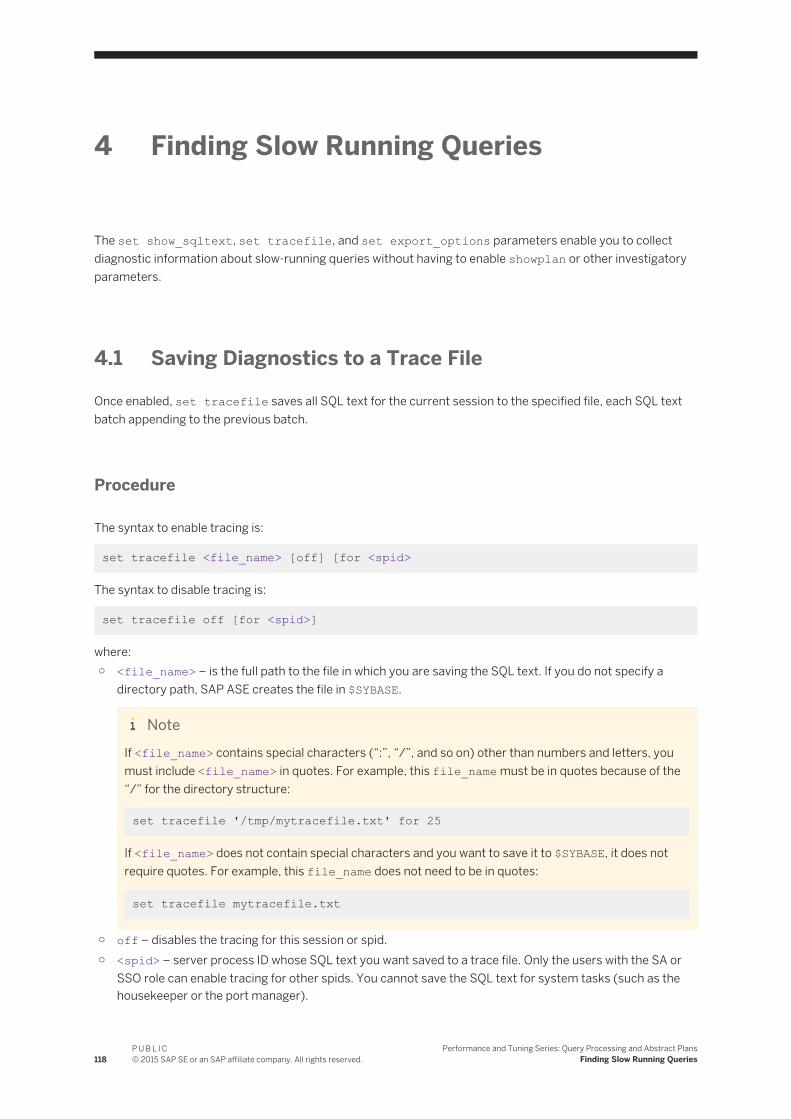
4 Finding Slow Running Queries
The set show_sqltext, set tracefile, and set export_options parameters enable you to collect diagnostic information about slow-running queries without having to enable showplan or other investigatory parameters.
4.1 Saving Diagnostics to a Trace File
Once enabled, set tracefile saves all SQL text for the current session to the specified file, each SQL text batch appending to the previous batch.
Procedure
The syntax to enable tracing is:
set tracefile <file_name> [off] [for <spid>
The syntax to disable tracing is:
set tracefile off [for <spid>]
where:○ <file_name> – is the full path to the file in which you are saving the SQL text. If you do not specify a
directory path, SAP ASE creates the file in $SYBASE.
NoteIf <file_name> contains special characters (“:”, “/”, and so on) other than numbers and letters, you must include <file_name> in quotes. For example, this file_name must be in quotes because of the “/” for the directory structure:
set tracefile '/tmp/mytracefile.txt' for 25
If <file_name> does not contain special characters and you want to save it to $SYBASE, it does not require quotes. For example, this file_name does not need to be in quotes:
set tracefile mytracefile.txt
○ off – disables the tracing for this session or spid.○ <spid> – server process ID whose SQL text you want saved to a trace file. Only the users with the SA or
SSO role can enable tracing for other spids. You cannot save the SQL text for system tasks (such as the housekeeper or the port manager).
118P U B L I C© 2015 SAP SE or an SAP affiliate company. All rights reserved.
Performance and Tuning Series: Query Processing and Abstract PlansFinding Slow Running Queries

Examples:○ This example opens a trace file named sql_text_file for the the current session:
set tracefile '/var/sybase/REL1502/text_dir/sql_text_file'
Subsequent outputs from set showplan, set statistics io, and dbcc traceon(100) are saved in sql_text_file.
○ This example does not specify a directory path, so the trace file is saved in $SYBASE/sql_text_file:
set tracefile 'sql_text_file' for 11
Any SQL run on spid 11 is saved to this tracefile.○ This example saves the SQL text for spid 86:
set tracefile '/var/sybase/REL1502/text_dir/sql_text_file' for 86
○ This example disables set tracefile:
set tracefile off
These are the restrictions for set tracefile:○ You cannot save the SQL text for system tasks (such as the housekeeper or the port manager).○ You must have the sa or sso roles, or be granted set tracing permission, to run enable or disable
tracing.○ set tracefile is not allowed to open an existing file as a tracefile.○ During an SA or SSO session, if you enable set tracfile for a specific spid, all subsequent tracing
commands executed take effect on that spid, not the SA or SSO spid.○ If SAP ASE runs out of file space while writing the tracefile, it closes the file and disables the tracing.○ If an isql session starts tracing for a spid, but the isql session quits without disabling the tracing,
another isql session can begin tracing this spid.○ Tracing occurs for the session for which it is enabled only, not for the session that enabled it.○ You cannot trace more than one session at a time from a single sa or sso session. If you attempt to open a
tracefile for a session for which there is already a trace file open, SAP ASE issues this error message: tracefile is already open for this session.
○ You cannot trace the same session from multiple sa or sso sessions.○ The file storing the trace output is closed when the session being traced quits or when you disable tracing.○ Before you allocate resources for tracing, keep in mind that each tracing requires one file descriptor per
engine.
4.1.1 set Options That Save Diagnostic Information to a Trace File
You can use set tracefile with other set commands and options that provide diagnostic information.
These set commands and options save diagnostic information to a file:
● set show_sqltext [on | off]● set showplan [on | off]
Performance and Tuning Series: Query Processing and Abstract PlansFinding Slow Running Queries
P U B L I C© 2015 SAP SE or an SAP affiliate company. All rights reserved. 119

● set statistics io [on | off]● set statistics time [on | off]● set statistics plancost [on | off]
These are the set options:
● set option show [normal | brief | long | on | off]● set option show_lop [normal | brief | long | on | off]● set option show_parallel [normal | brief | long | on | off]● set option show_search_engine [normal | brief | long | on | off]● set option show_counters [normal | brief | long | on | off]● set option show_managers [normal | brief | long | on | off]● set option show_histograms [normal | brief | long | on | off]● set option show_abstract_plan [normal | brief | long | on | off]● set option show_best_plan [normal | brief | long | on | off]● set option show_code_gen [normal | brief | long | on | off]● set option show_pio_costing [normal | brief | long | on | off]● set option show_lio_costing [normal | brief | long | on | off]● set option show_log_props [normal | brief | long | on | off]● set option show_elimination [normal | brief | long | on | off]
4.1.2 Determining the Traced Sessions
Use sp_helpapptrace to determine which sessions are being traced.
Context
sp_helpapptrace returns the server process IDs (spids) for all the sessions SAP ASE is tracing, the spids of the sessions tracing them, and the name of the trace file.
Procedure
The syntax for sp_helpapptrace is:
sp_helpapptrace
sp_helpapptrace returns these columns:○ traced_spid – spid of the session you are tracing.○ tracer_spid – spid of the session that traced_spid is tracing. Prints “exited” if the tracer_spid
session has exited.
120P U B L I C© 2015 SAP SE or an SAP affiliate company. All rights reserved.
Performance and Tuning Series: Query Processing and Abstract PlansFinding Slow Running Queries

○ trace_file – full path to the tracefile.
For example:
sp_helpapptrace
traced_spid tracer_spid trace_file -------------- ------------- ----------11 exited /tmp/myfile1 13 14 /tpcc/sybase.15_0/myfile2
If a session is tracing another session, but quits without disabling the tracing, SAP ASE allows a new session to rebind with the earlier trace. This means that a sa or sso is not required to finish every trace they start, but can start a trace session, quit, and then rebind to this trace session
4.2 Displaying SQL Text
set show_sqltext allows you to print the SQL text for ad hoc queries, stored procedures, cursors, and dynamic prepared statements.
Context
You do not need to enable the set show_sqltext before you execute the query (as you do with commands like set showplan on) to collect diagnostic information for a SQL session. Instead you can enable it while the commands are running to help determine which query is performing poorly and diagnose their problems.
Procedure
Before you enable show_sqltext, you must first enable dbcc traceon to display the output to standard out:
dbcc traceon(3604)
The syntax for set show_sqltext is:
set show_sqltext {on | off}
For example, this enables show_sqltext:
set show_sqltext on
Once set show_sqltext is enabled, SAP ASE prints all SQL text to standard out for each command or system procedure you enter. Depending on the command or system procedure you run, this output can be extensive.
Performance and Tuning Series: Query Processing and Abstract PlansFinding Slow Running Queries
P U B L I C© 2015 SAP SE or an SAP affiliate company. All rights reserved. 121

For example, if you run sp_who, SAP ASE prints all SQL text associated with this system procedure (the output is abbreviated for space purposes):
sp_who 2007/02/23 02:18:25.77SQL Text: sp_whoSproc: sp_who, Line: 0Sproc: sp_who, Line: 20Sproc: sp_who, Line: 22Sproc: sp_who, Line: 25Sproc: sp_who, Line: 27Sproc: sp_who, Line: 30Sproc: sp_who, Line: 55Sproc: sp_who, Line: 64Sproc: sp_autoformat, Line: 0Sproc: sp_autoformat, Line: 165Sproc: sp_autoformat, Line: 167Sproc: sp_autoformat, Line: 177Sproc: sp_autoformat, Line: 188. . . Sproc: sp_autoformat, Line: 326Sproc: sp_autoformat, Line: 332SQL Text: INSERT #colinfo_af(colid,colname,usertype,type,typename,collength,maxlength,autoformat,selected,selectorder,asname,mbyte) SELECT c.colid,c.name,t.usertype,t.type,t.name,case when c.length < 80 then 80 else c.length end,0,0,0,0,c.name,0 FROM tempdb.dbo.syscolumns c,tempdb.dbo.systypes t WHERE c.id=1949946031 AND c.usertype=t.usertypeSproc: sp_autoformat, Line: 333Sproc: sp_autoformat, Line: 334. . . Sproc: sp_autoformat, Line: 535Sproc: sp_autoformat, Line: 0Sproc: sp_autoformat, Line: 393Sproc: sp_autoformat, Line: 395. . . Sproc: sp_autoformat, Line: 686Sproc: sp_autoformat, Line: 688SQL Text: UPDATE #colinfo_af SET maxlength=(SELECT isnull(max(isnull(char_length(convert(varchar(80),fid)),4)),1) FROM #who1result ), autoformat = 1, mbyte=case when usertype in (24, 25, 34, 35) then 1 else 0 end WHERE colname='fid'Sproc: sp_autoformat, Line: 689Sproc: sp_autoformat, Line: 690. . .Sproc: sp_autoformat, Line: 815Sproc: sp_autoformat, Line: 818 SQL Text: SELECT fid=right(space(80)+isnull(convert(varchar(80),fid),'NULL'),3), spid=right(space(80)+isnull(convert(varchar(80),spid),'NULL'),4), status=SUBSTRING(convert(varchar(80),status),1,8), loginame=SUBSTRING(convert(varchar(80),loginame),1,8), origname=SUBSTRING(convert(varchar(80),origname),1,8), hostname=SUBSTRING(convert(varchar(80),hostname),1,8), blk_spid=right(space(80)+isnull(convert(varchar(80),blk_spid),'NULL'),8), dbname=SUBSTRING(convert(varchar(80),dbname),1,6), tempdbname=SUBSTRING(convert(varchar(80),tempdbname),1,10), cmd=SUBSTRING(convert(varchar(80),cmd),1,17), block_xloid=right(space(80)+isnull(convert(varchar(80),block_xloid),'NULL'),11) FROM #who1result order by fid, spid, dbname
Sproc: sp_autoformat, Line: 819 Sproc: sp_autoformat, Line: 820Sproc: sp_autoformat, Line: 826Sproc: sp_who, Line: 68Sproc: sp_who, Line: 70
122P U B L I C© 2015 SAP SE or an SAP affiliate company. All rights reserved.
Performance and Tuning Series: Query Processing and Abstract PlansFinding Slow Running Queries

fid spid status loginame origname hostname blk_spid dbname tempdbnamecmd block_xloid--- ---- -------- -------- -------- -------- -------- ------------------------- ----------- 0 2 sleeping NULL NULL NULL 0 master tempdbDEADLOCK TUNE 0 0 3 sleeping NULL NULL NULL 0 master tempdbASTC HANDLER 00 4 sleeping NULL NULL NULL 0 master tempdbCHECKPOINT SLEEP 00 5 sleeping NULL NULL NULL 0 master tempdbHK WASH 00 6 sleeping NULL NULL NULL 0 master tempdbHK GC 00 7 sleeping NULL NULL NULL 0 master tempdbHK CHORES 00 8 sleeping NULL NULL NULL 0 master tempdbPORT MANAGER 00 9 sleeping NULL NULL NULL 0 master tempdbNETWORK HANDLER 00 10 sleeping NULL NULL NULL 0 master tempdbLICENSE HEARTBEAT 00 1 running sa sa echo 0 master tempdbINSERT 0(10 rows affected) (return status = 0)
To disable show_sqltext, enter:
set show_sqltext off
Restrictions for show_sqltext:○ You must have the sa or sso roles to run show_sqltext.○ You cannot use show_sqltext to print the SQL text for triggers.○ You cannot use show_sqltext to show a binding variable or a view name.
4.3 Retaining Session Settings
By default, any set parameter changes that are set by a trigger or system procedure are reset when they finish running.
Procedure
Enable set export_options to export the session settings set by a system procedure or trigger to the parent (or issuer) of the stored procedure or trigger. In this example, SAP ASE exports set showplan on to outer_proc, but does not exported it to a parent stored procedure:
create proc inner_proc as set showplan on select * from titles set export_options on
Performance and Tuning Series: Query Processing and Abstract PlansFinding Slow Running Queries
P U B L I C© 2015 SAP SE or an SAP affiliate company. All rights reserved. 123

go create proc outer_proc as exec inner_proc go
124P U B L I C© 2015 SAP SE or an SAP affiliate company. All rights reserved.
Performance and Tuning Series: Query Processing and Abstract PlansFinding Slow Running Queries

5 Parallel Query Processing
Query execution supports both horizontal and vertical parallelism.
Vertical parallelism is the ability to run multiple operators simultaneously by employing different system resources such as CPUs, disks, and so on. Horizontal parallelism is the ability to run multiple instances of an operator on the specified portion of the data.
The way you partition your data greatly affects the efficiency of horizontal parallelism. The logical partitioning of data is useful in operational decision-support systems (DSS) queries where large volumes of data are being processed.
See Transact-SQL Users Guide > Partitioning Tables and Indexes and the Performance and Tuning Series: Physical Database Tuning guide for a more detailed discussion of partitioning on SAP ASE. Understanding different types of partitioning is a prerequisite to understanding this chapter.
SAP ASE also supports pipelined parallelism. Pipelining is a form of vertical parallelism in which intermediate results are piped to higher operators in a query tree. The output of one operator is used as input for another operator. The operator used as input can run simultaneously with the operator feeding the data, which is an essential element in pipelined parallelism. Use parallelism only when multiple resources like disks and CPUs are available. Using parallelism can be detrimental if your system is not configured for resources that can work in tandem. In addition, data must be spread across disk resources in a way that closely ties the logical partitioning of the data with the physical partitioning on parallel devices. The biggest challenge for a parallel system is to control the correct granularity of parallelism. If parallelism is too finely grained, communication and synchronization overhead can offset any benefit that is obtained from parallel operations. Making parallelism too coarse does not permit proper scaling.
5.1 Queries That Benefit from Parallel Processing
When SAP ASE is configured for parallel query processing, the query optimizer evaluates each query to determine whether it is eligible for parallel execution.
If it is eligible, and if the optimizer determines that a parallel query plan can deliver results faster than a serial plan, the query is divided into plan fragments that are processed simultaneously. The results are combined and delivered to the client in a shorter period of time than it takes to process the query serially as a single fragment. Parallel query processing can improve the performance of:
● select statements that scan large numbers of pages but return relatively few rows, such as table scans or clustered index scans with grouped or ungrouped aggregates.
● Table scans or clustered index scans that scan a large number of pages, but have where clauses that return only a small percentage of rows.
● select statements that include union, order by, or distinct, since these query operations can make use of parallel sorting or parallel hashing.
● select statements where a reformatting strategy is chosen by the optimizer, since these can populate worktables in parallel and can make use of parallel sorting.
Performance and Tuning Series: Query Processing and Abstract PlansParallel Query Processing
P U B L I C© 2015 SAP SE or an SAP affiliate company. All rights reserved. 125

● join queries.
Commands that return large, unsorted result sets are unlikely to benefit from parallel processing due to network constraints. In most cases, results can be returned from the database faster than they can be merged and returned to the client over the network.
Parallel DMLs like insert, delete, and update are not supported and so do not benefit from parallelism.
5.2 Enabling Parallelism
Enable the number of worker processes and max parallel degree parameters to configure SAP ASE for parallelism.
To gain optimal performance, be aware of other configuration parameters that affect the quality of plans.
5.2.1 Setting the Number of Worker Processes
Before you enable parallelism, configure the number of worker processes (also referred to as threads) available by setting the configuration parameter number of worker processes.
Context
SAP recommends that you set the value for number of worker processes to one and a half times the total number required at peak load. You can calculate an approximate number using the max parallel degree configuration parameter, which indicates the total number of worker processes that can be used for any query. Depending on the number of connections to the SAP ASE and the approximate number of queries that are run simultaneously, you can use this rule to roughly estimate the value for the number of worker processes that may be needed at any time:
[number of worker processes] = [max parallel degree] X [the number of concurrent connections wanting to run queries in parallel] X [1.5]
Procedure
For example, to set the number of worker processes to 40:
sp_configure "number of worker processes", 40
Any runtime adjustment for the number of threads may have a negative effect on query performance. SAP ASE always tries to optimize thread usage, but it may have already committed to a plan that needs increased resources, and therefore does not guarantee a linear scaledown when it runs with fewer threads.
126P U B L I C© 2015 SAP SE or an SAP affiliate company. All rights reserved.
Performance and Tuning Series: Query Processing and Abstract PlansParallel Query Processing

If the query processor has insufficient worker processes, the processor tries to adjust the query plan during runtime. If a minimal number of worker processes are required but unavailable, the query aborts with this error message:
Insufficient number of worker processes to execute the parallel query. Increase the value of the configuration parameter ‘number of worker processes’
5.2.2 Setting max parallel degree
Use the max parallel degree configuration parameter to configure the maximum amount of parallelism for a query.
Context
This parameter determines the maximum number of threads used to process a a given query.
Procedure
For example, to set max parallel degree to 10, enter:
sp_configure "max parallel degree", 10
Unlike versions earlier than 15.0, this parameter’s value is not entirely enforced by the query optimizer. A complete enforcement process is expensive in terms of optimization time. SAP ASE comes close to the desired setting of max parallel degree and exceeds it only for semantic reasons to guarantee correctness.
5.2.3 Setting max resource granularity
The value of max resource granularity configures the maximum percentage of system resources a query can use.
Context
By default, max resource granularity is 10%. The query engine can avoid memory-intensive strategies, such as hash-based algorithms, when you set max resource granularity to a low value. The optimizer uses max resource granularity to limit the estimated resources in query plan selection, including buffers used in sorting and hashing, and the number of buffers that can be used in the query plan.
Performance and Tuning Series: Query Processing and Abstract PlansParallel Query Processing
P U B L I C© 2015 SAP SE or an SAP affiliate company. All rights reserved. 127

Procedure
To set max resource granularity to 5%, enter:
sp_configure "max resource granularity", 5
If the the query processor’s search engine has consumed more than the configured percentage of procedure cache, and if it has found at least one full plan, the search engine times out and uses the current best plan for the query.
If the query processor does not find a full plan before reaching the value for max resource granularity as a percentage of procedure cache, the search engine continues to search until it finds the next full plan. However, if the search engine reaches 50% of the complete procedure cache and finds no plan, it aborts the query compilation to avoid shutting down the server.
The execution engine uses max resource granularity to limit the number of buffers used during dynamic buffer allocation. Hash-based update statistics uses max resource granularity to limit the amount of tempdb buffer cache used.
5.2.4 Setting max repartition degree
SAP ASE must dynamically repartition intermediate data to match the partitioning scheme of another operand, or to perform an efficient partition elimination.
Context
max repartition degree controls the amount of dynamic repartitioning. If the value of max repartition degree is too high, the number of intermediate partitions could become too large and the system could become flooded with worker processes that compete for resources, which eventually degrades performance. The value for max repartition degree enforces the maximum number of partitions created for any intermediate data. Repartitioning is a CPU-intensive operation. The value of max repartition degree should not exceed the total number of SAP ASE engines.
If all tables and indexes are unpartitioned, SAP ASE uses the value for max repartition degree to provide the number of partitions to create as a result of repartitioning the data. When the value is set to 1, which is the default case, the value of max repartition degree is set to the number of online engines.
Procedure
Use max repartition degree when using the force option to perform a parallel scan on a table or index:
select * from customers (parallel)
For example, if the customers table is unpartitioned and the force option is used, SAP ASE tries to find the inherent partitioning degree of that table or index, which in this case is 1. It uses the number of engines
128P U B L I C© 2015 SAP SE or an SAP affiliate company. All rights reserved.
Performance and Tuning Series: Query Processing and Abstract PlansParallel Query Processing

configured for the server, or whatever degree is best based on the number of pages in the table or index that does not exceed the value of max repartition degree.
To set max repartition degree to 5:
sp_configure "max repartition degree", 5
5.2.5 Setting max scan parallel degree
The max scan parallel degree configuration parameter is used only for backward compatibility, when the data in a partitioned table or index is highly skewed.
Context
If the value of this parameter is greater than 1, SAP ASE uses this value to do a hash-based parallel scan. The value of max scan parallel degree cannot exceed the value of max parallel degree.
5.2.6 Setting prod-consumer overlap factor
prod-consumer overlap factor affects how much pipelined parallelism can be created in a query plan.
Context
The default value is 20%, which means that if two operators in a parent-child relationship are run by separate worker processes, there is a 20% overlap. The remaining 80% of the operation is sequential. This affects the way in which SAP ASE costs two plan fragments. Consider the example of a scan operator under a grouping operation.
Procedure
In such a case, if the scan operator takes <N1> seconds and grouping operations take <N2> seconds, the response time of the two operators is:
0.2 * max (N1, N2) + 0.8 * (N1 + N2)
In setting this parameter, consider the number of online engines on which SAP ASE is running and the complexity of the queries to be run. As a general rule, use thread resources to scan on multiple partitions first. Then, if there are unused thread resources, use them to speed up vertical pipelined parallelism. Do not exceed a value of 50.
Performance and Tuning Series: Query Processing and Abstract PlansParallel Query Processing
P U B L I C© 2015 SAP SE or an SAP affiliate company. All rights reserved. 129

5.2.7 Setting min pages for parallel scan
max pages for parallel scan controls the tables and indexes that can be accessed in parallel.
Context
If the number of pages in a table is below this value, the table is accessed serially. The default value is 200 pages; page size is not relevant. Although the tables and indexes of the table are accessed serially, SAP ASE tries to repartition the data, if that is appropriate, and to use parallelism above the scans, if that is appropriate.
5.2.8 Setting max query parallel degree
max query parallel degree defines the number of worker processes to use for a given query.
Context
This parameter is relevant only if you do not want to enable parallelism globally.
Procedure
You must configure the number of worker processes to a value greater than zero, but max query parallel degree must be set to 1.
When max query parallel degree is set to a value greater than 1, queries are not compiled to use parallelism. Instead, you can specify parallel hints, using abstract plans to compile one or more queries using parallelism.
Use use parallel <N> to define how much parallelism is to be used for a given query. Alternatively, use create plan to specify the query and the number of worker processes to use for it.
130P U B L I C© 2015 SAP SE or an SAP affiliate company. All rights reserved.
Performance and Tuning Series: Query Processing and Abstract PlansParallel Query Processing

5.3 Controlling Parallelism at the Session Level
The set options let you restrict the degree of parallelism on a session basis, in stored procedures, or in triggers.
Context
These options are useful for tuning experiments with parallel queries and can also be used to restrict noncritical queries to run in serial, so that worker processes remain available for other tasks.
Table 5: Session-Level Parallelism Control Parameters
Parameter Function
parallel_degree Sets the maximum number of worker processes for a query in a session, stored procedure, or trigger. Overrides the max parallel degree configuration parameter, but must be less than or equal to the value of max parallel degree.
scan_parallel_degree
Sets the maximum number of worker processes for a hash-based scan during a specific session, stored procedure, or trigger. Overrides the max scan parallel degree configuration parameter and must be less than or equal to the value of max scan parallel degree.
resource_granularity
Overrides the global value max resource granularity and sets it to a session-specific value, which influences whether SAP ASE uses memory-intensive operations.
repartition_degree
Sets the value of max repartition degree for a session. This is the maximum degree to which any intermediate data stream is be repartitioned for semantic purposes.
If you specify a value that is too large for any of the set options, the value of the corresponding configuration parameter is used, and a message reports the value that is in effect. While set parallel_degree, set scan_parallel_degree, set repartition_degree, or set resource_granularity is in effect during a session, the plans for any stored procedures that you execute are not placed in the procedure cache. Procedures executed with these set options in effect may produce less than optimal plans.
Procedure
This example restricts all queries started in the current session to 5 worker processes:
set parallel_degree 5
While this command is in effect, any query on a table with more than 5 partitions cannot use a partition-based scan, unless you enable dynamic thread assignment. Dynamic thread assignment allows a thread to scan other partitions after it completes working on its current partition.
Performance and Tuning Series: Query Processing and Abstract PlansParallel Query Processing
P U B L I C© 2015 SAP SE or an SAP affiliate company. All rights reserved. 131

To remove the session limit, use:
set parallel_degree 0
or:
set scan_parallel_degree 0
To run subsequent queries in serial mode, use:
set parallel_degree 1
or:
set scan_parallel_degree 1
To set resource granularity to 25% of the total resources available in the system, use:
set resource_granularity 25
The same is true for repartition degree as well; you can set it to a value of 5. It cannot, however, exceed the value of max parallel degree.
set repartition_degree 5
5.4 Controlling Query Parallelism
The parallel extension to the from clause of a select command allows users to suggest the number of worker processes used in a select statement.
Context
The degree of parallelism that you specify cannot be more than the value set with sp_configure or the session limit controlled by a set command. If you specify a higher value, the specification is ignored, and the optimizer uses the set or sp_configure limit.
The syntax for the select statement is:
select ...from <tablename> [( [index <index_name>] [parallel [<degree_of_parallelism> | 1 ]] [prefetch <size>] [lru|mru] ) ] , <tablename> [( [index <index_name>] [parallel [<degree_of_parallelism> | 1] [prefetch <size>] [lru|mru] ) ] ...
132P U B L I C© 2015 SAP SE or an SAP affiliate company. All rights reserved.
Performance and Tuning Series: Query Processing and Abstract PlansParallel Query Processing

Procedure
To specify the degree of parallelism for a single query, include parallel after the table name. This example executes in serial:
select * from huge_table (parallel 1)
This example specifies the index to use in the query, and sets the degree of parallelism to 2:
select * from huge_table (index ncix parallel 2)
5.5 Using Parallelism Selectively
Not all queries benefit from parallelism. In general, the optimizer determines which queries will not benefit from parallelism and attempts to run them serially.
Context
When the query processor makes errors in such cases, it is usually because of skewed statistics or incorrect costing as a result of imperfect modeling. Experience will show you whether queries are running better or worse, and you can decide to keep parallel on or off.
If you keep parallel on, and have identified the queries you want to run in serial mode, you can attach an abstract plan hint, as follows:
select count(*) from sysobjects plan “(use parallel 1)”
The same effect is achieved by creating a query plan:
create plan “select count(*) from sysobjects” “use parallel 1”
If, however, you notice that parallelism is resource-intensive or that it does not generate query plans that perform well, use it selectively.
To enable parallelism for selected complex queries:
Procedure
1. Set the number of worker processes to a number greater than zero. For example, to configure 10 worker processes, execute:
sp_configure “number of worker processes”, 10
Performance and Tuning Series: Query Processing and Abstract PlansParallel Query Processing
P U B L I C© 2015 SAP SE or an SAP affiliate company. All rights reserved. 133

2. Set max query parallel degree to a value greater than 1. As a starting point, set it to what you would have used for max parallel degree:
sp_configure “max query parallel degree”, 10
3. The preferred way to force a query to use a parallel plan is to use the abstract plan syntax:
use parallel <N>
where <N> is less than the value of max query parallel degree.
4. To write a query that uses a maximum of 5 threads, use:
select count (*), S1.id from sysobjects S1, sysindexes S2 where S1.id = S2.idgroup by S1.idplan “(use parallel 5)”
This query tells the optimizer to use 5 worker processes, if it can. the only drawback to this approach is that you must alter the actual queries in the application. To avoid this, use create plan:
create plan “select count(*),S1.id from sysobjects S1,sysindexes S2where S1.id = S2.idgroup by S1.id” “(use parallel 5)”
To turn the abstract plan load option on globally, enter:
sp_configure “abstract plan load”, 1
5.6 Using Parallelism with Large Numbers of Partitions
The information in this section also applies when partitioning is configured for manageability, and when partitions are created on physical or logical devices that exhibit little or no parallelism.
Context
For the purpose of this discussion, you have decided to partition a table using range partitioning that represents each week of a year. The issue here is that the query optimizer does not know how the underlying disk system will respond to a 52-way parallel scan. The optimizer must determine the best way to scan the table. If there are enough worker processes configured, the optimizer uses 52 threads to scan the table, which may well cause serious performance issues and be even slower than a serial scan.
134P U B L I C© 2015 SAP SE or an SAP affiliate company. All rights reserved.
Performance and Tuning Series: Query Processing and Abstract PlansParallel Query Processing

Procedure
1. To prevent this, first find out exactly how much parallelism is supported. If you know the devices that are used for this table, you can use the following command on a UNIX system, where the underlying device is called </dev/xx>:
time dd if=/dev/xx of=/dev/null bs=2k skip=8 count = 102400 &
Assume that time records as <x>.
2. Now run two of the same commands concurrently:
time dd if=/dev/xx of=/dev/null bs=2k skip=8 count = 102400 &
3. This time, assume that time is <y>. In a linear scale-up, <x> is the same as <y>, which is probably impossible to achieve. The following identity may suffice:
<x> <=< y> <= (<N>*x)/<k>
Where <N> is the number of simultaneous sessions started and <k> is a constant that identifies an acceptable improvement level. A good approximation of <k> might be 1.4, which says that parallel scan is allowed as long as it delivers 40% better metrics than a serial scan.
Table 6: Parallel scan metrics
Number of Threads Performance Metrics Acceptable for k=1.4
1 200s
2 245s 245 <= (200*2)/1.4; i.e. 245<=285.71
4 560s 560 <= (200*4)/1.4; i.e. 560<=571.42
5 725s 725 <= (200*5)/1.4; i.e. 725<=714.28
This table shows that the disk subsystem did not perform well after four concurrent accesses; the performance numbers went below the acceptable limit established by <k>. In general, read enough data blocks to allow for any skewed readings.
Having established that 4 threads is optimal, provide this hint by binding it to the object using sp_chgattribute in this way:
sp_chgattribute <<tablename>>, “plldegree”, 4
This tells the query optimizer to use a maximum of four threads. It may choose fewer than four threads if it does not find enough resources. The same mechanism can be applied to an index. For example, if an index called auth_ind exists on authors and you want to use two threads to access it, use:
sp_chgattribute “authors.auth_ind”, “plldegree”, 2
You must run sp_chgatttribute from the current database.
Performance and Tuning Series: Query Processing and Abstract PlansParallel Query Processing
P U B L I C© 2015 SAP SE or an SAP affiliate company. All rights reserved. 135

5.7 When Parallel Query Results Differ
When a query does not include scalar aggregates or require a final sorting step, a parallel query might return results in a different order from the same query run in serial, and subsequent executions of the same query in parallel might return results in different orders.
The relative speed of the different worker processes leads to differences in result-set ordering. Each parallel scan behaves differently, due to pages already in cache, lock contention, and so forth. Parallel queries always return the same set of results, just not in the same order.
NoteIf you need a dependable ordering of results, use order by, or run the query in serial mode.
In addition, due to the pacing effects of multiple worker processes reading data pages, two types of queries accessing the same data may return different results when an aggregate or a final sort is not done. They are:
● Queries that use set rowcount● Queries that select a column into a local variable without sufficiently restrictive query clauses
5.7.1 Queries That Use set rowcount
The set rowcount option stops processing from continuing after a certain number of rows are returned to the client.
With serial processing, the results are consistent in repeated executions as long as the query plans are the same. In serial mode, given the same query plan, the same rows are returned in the same order for a given rowcount value, because a single process reads the data pages in the same order every time. With parallel queries, the order of the results and the set of rows returned can differ, because worker processes may access pages sooner or later than other processes. To get consistent results, either use a clause that performs a final sort step, or run the query in serial.
5.7.2 Queries That Set Local Variables
You can set the value of a local variable in a select statement.
Procedure
For example:
select @tid = title_id from titles where type = "business"
136P U B L I C© 2015 SAP SE or an SAP affiliate company. All rights reserved.
Performance and Tuning Series: Query Processing and Abstract PlansParallel Query Processing

The where clause matches multiple rows in the titles table, so the local variable is always set to the value from the last matching row returned by the query. The value is always the same in serial processing, but for parallel query processing, the results depend on which worker process finishes last. To achieve a consistent result, use a clause that performs a final sort step, execute the query in serial mode, or add clauses so that the query arguments select only single rows.
5.8 Understanding Parallel Query Plans
The key to understanding parallel query processing is to understand the basic building blocks in a parallel query plan.
NoteSee Using showplan for an explanation of how to display a query plan in a text-based format for each SQL statement in a batch or stored procedure.
A compiled query plan contains a tree of execution operators that closely resembles the relational semantics of the query. Each query operator implements a relational operation using a specific algorithm. For example, a query operator called the nested-loop join implements the relational join operation. In SAP ASE, the primary operator for parallelism is the exchange operator, which is a control operator that does not implement any relational operation. An exchange operator creates new worker processes that can handle fragments of data. During optimization, SAP ASE strategically places the exchange operator to create operator tree fragments that can run in parallel. All operators found below the exchange operator (down to the next exchange operator) are executed by worker threads that clone the fragment of the operator tree to produce data in parallel. The exchange operator can then redistribute this data to the parent operator above it in the query plan. The exchange operator handles the pipelining and rerouting of data.
In the following sections, the word “degree” is used in two different contexts. When “degree N” of a table or index is referred to, it references the number of partitions contained in a table or index. When the “degree of an operation” or “the degree of a configuration parameter” is referred to, it references the number of partitions generated in the intermediate data stream.
The following example shows how operators in the query processor work in serial with the following query run in the pubs2 database. The table titles is hash-partitioned three ways on the column pub_id.
select * from titles QUERY PLAN FOR STATEMENT 1 (at line 1).1 operator(s) under rootThe type of query is SELECT.ROOT:EMIT Operator |SCAN Operator | FROM TABLE | titles | Table Scan. | Forward Scan. | Positioning at start of table. | Using I/O Size 2 Kbytes for data pages. | With LRU Buffer Replacement Strategy for data pages.
Performance and Tuning Series: Query Processing and Abstract PlansParallel Query Processing
P U B L I C© 2015 SAP SE or an SAP affiliate company. All rights reserved. 137

As this example illustrates, the titles table is being scanned by the scan operator, the details of which appear in the showplan output. The emit operator reads the data from the scan operator and sends it to the client application. A given query can create an arbitrarily complex tree of such operators.
When parallelism is enabled, SAP ASE can perform a simple scan in parallel using the exchange operator above the scan operator. The exchange operator produces three worker processes (based on the three partitions), each of which scans the three disjointed parts of the table and sends the output to the consumer process. The emit operator at the top of the tree does not know that the scans are done in parallel.
Example A:
select * from titles
Executed in parallel by coordinating process and 3 worker processes. 4 operator(s) under rootThe type of query is SELECT.ROOT:EMIT Operator |EXCHANGE Operator (Merged) |Executed in parallel by 3 Producer and 1 Consumer processes. | | |EXCHANGE:EMIT Operator | | | | |RESTRICT Operator | | | | | | |SCAN Operator | | | | FROM TABLE | | | | titles | | | | Table Scan. | | | | Forward Scan. | | | | Positioning at start of table. | | | | Executed in parallel with a 3-way partition scan. | | | | Using I/O Size 2 Kbytes for data pages. | | | | With LRU Buffer Replacement Strategy for data pages.
The operator called EXCHANGE:EMIT is placed under an EXCHANGE operator to route data up to its parent EXCHANGE operator.
Related Information
Using showplan [page 49]EXCHANGE Operator [page 139]
138P U B L I C© 2015 SAP SE or an SAP affiliate company. All rights reserved.
Performance and Tuning Series: Query Processing and Abstract PlansParallel Query Processing

5.9 Parallel Query Execution Model
One of the key components of the parallel query execution model is the EXCHANGE operator. You can see it in the showplan output of a query.
5.9.1 EXCHANGE Operator
The EXCHANGE operator marks the boundary between a producer and a consumer operator (the operators below the EXCHANGE operator produce data and those above it consume data).
In example A, above, which showed a parallel scan of the titles table (select * from titles), the EXCHANGE:EMIT and the SCAN operators produce data. This is shown briefly.
select * from titles The type of query is SELECT.ROOT:EMIT Operator |EXCHANGE Operator (Merged) |Executed in parallel by 3 Producer and 1 Consumer processes. | | |EXCHANGE:EMIT Operator | | | | |RESTRICT Operator | | | | | | |SCAN Operator | | | | FROM TABLE | | | | titles | | | | Table Scan.
This figure shows the process boundary between a producer and a consumer process. In this example, one consumer process reads data from a pipe (which is used as a medium to transfer data across process boundaries) and passes the data to the emit operator, which in turn routes the result to the client. The exchange operator also spawns worker processes, which are called producer threads. The exchange:emit operator writes the data into a pipe managed by the exchange operator.
Performance and Tuning Series: Query Processing and Abstract PlansParallel Query Processing
P U B L I C© 2015 SAP SE or an SAP affiliate company. All rights reserved. 139

There are two plan fragments in this query plan. The plan fragment with the scan and the exchange:emit operators are cloned three ways and then a three-to-one exchange operator writes it into a pipe. The emit operator and the exchange operator are run by a single process, which means there is a single clone of that plan fragment.
Pipe Management
The four types of pipes managed by the exchange operator are distinguished by how they split and merge data streams.
You can determine which type of pipe is being managed by the exchange operator by looking at its description in the showplan output, where the number of producers and consumers are shown. The four pipe types are described below:
● Many-to-one – the exchange operator spawns multiple producer threads and has one consumer task that reads the data from a pipe, to which multiple producer threads write. The exchange operator in the previous example implements a many-to-one exchange. A many-to-one exchange operator can be order-preserving and this technique is employed particularly when doing a parallel sort for an order by clause. The producer's sorted data streams are merged into a single, final, ordered data stream for the consumer. The showplan output shows more than one producer process and one consumer process.
|EXCHANGE Operator (Merged) |Executed in parallel by 3 Producer and 1 Consumer processes
● One-to-many – there is one producer and multiple consumer threads. The producer thread writes data to multiple pipes according to a partitioning scheme devised at query optimization, and then routes data to each of these pipes. Each consumer thread reads data from one of the assigned pipes. This kind of data
140P U B L I C© 2015 SAP SE or an SAP affiliate company. All rights reserved.
Performance and Tuning Series: Query Processing and Abstract PlansParallel Query Processing

split can preserve the ordering of the data. The showplan output shows one producer process and more than one consumer processes:
|EXCHANGE Operator (Repartitioned) |Executed in parallel by 1 Producer and 4 Consumer processes
● Many-to-many – there are multiple producers and multiple consumers. Each producer writes to multiple pipes, and each pipe has multiple consumers. Each stream is written to a pipe. Each consumer thread reads data from one of the assigned pipes.
|EXCHANGE Operator (Repartitioned) |Executed in parallel by 3 Producer and 4 Consumer processes
● Replicated exchange operators – the producer thread writes all of its data to each pipe that the exchange operator configures. The producer thread makes a number of copies of the source data (the number is specified by the query optimizer) equal to the number of pipes in the exchange operator. Each consumer thread reads data from one of the assigned pipes. The showplan output shows this as follows:
|EXCHANGE (Replicated) |Executed in parallel by 3 Producer and 4 Consumer processes
5.9.1.1 Worker Process Model
A parallel query plan is composed of different operators, at least one of which is an exchange operator.
At runtime, a parallel query plan is bound to a set of server processes that, together, execute the query plan in a parallel fashion.
The server process associated with the user connection is called the alpha process because it is the source process from which parallel execution is initiated. In particular, each worker process involved in the execution of the parallel query plan is spawned by the alpha process.
In addition to spawning worker processes, the alpha process initializes all the worker processes involved in the execution of the plan, and creates and destroys the pipes necessary for worker processes to exchange data. The alpha process is, in effect, the global coordinator for the execution of a parallel query plan.
At runtime, SAP ASE associates each exchange operator in the plan with an initial set of worker processes. The worker processes execute the query plan fragment located immediately below the exchange operator.
For the query in Example A, the exchange operator is associated with three worker processes. Each worker process executes the plan fragment made of the exchange:emit operator and of the scan operator.
Performance and Tuning Series: Query Processing and Abstract PlansParallel Query Processing
P U B L I C© 2015 SAP SE or an SAP affiliate company. All rights reserved. 141

Each exchange operator is also associated with a server process named the beta process, which can be either the alpha process or a worker process. The beta process associated with a given exchange operator is the local coordinator for the execution of the plan fragment below the exchange operator. This is primarily relevant for query plans with multi-tiered or nested exchange operators. In the example above, the beta process is the same process as the alpha process, because the plan to be executed has only one level of exchange operators.
The following query illustrates what happens when the query plan contains multiple exchange operators:
select count(*),pub_id, pub_date from titles group by pub_id, pub_date
142P U B L I C© 2015 SAP SE or an SAP affiliate company. All rights reserved.
Performance and Tuning Series: Query Processing and Abstract PlansParallel Query Processing

There are two levels of exchange operators marked as EXCHANGE-1 and EXCHANGE-2 in the figure above. Worker process T4 is the beta process associated with the exchange operator EXCHANGE-2.
The beta process locally orchestrates execution of the plan fragment below the exchange operator; it dispatches query plan information that is needed by the worker processes, and synchronizes the execution of the plan fragment.
A process involved in the execution of a parallel query plan that is neither the alpha process nor a beta process is called a gamma process.
A given parallel query plan is bound at runtime to a unique alpha process, to one or more beta processes, and to at least one gamma process. Any SAP ASE parallel plan needs at least two different processes (alpha and gamma) to be executed in parallel.
To find out the mapping between exchange operators and worker processes, as well as to figure out which process is the alpha process, and which processes are the beta processes, use dbcc traceon(516):
=======Thread to XCHg Map BEGINS======= ALFA thread spid: 17XCHG = 2 <- refers to Xchg-2Comp Count = 2 Exec Count = 2 Range Adjustable Consumer XCHG = 5 Parent thread spid: 34 <- refers to T4 Child thread 0: spid:37 <- refers to T1 Child thread 1: spid: 38 <- refers to T2 Child thread 2: spid: 36 <- refers to T3 Scheduling level: 0
Performance and Tuning Series: Query Processing and Abstract PlansParallel Query Processing
P U B L I C© 2015 SAP SE or an SAP affiliate company. All rights reserved. 143

XCHG = 5 <- refers to Xchg-1 Comp Count = 3 Exec Count = 3Bounds Adjustable Consumer XCHG -1 Parent thread spid: 17 <- refers to Alpha Child thread 0: spid: 34 <- refers to T4 Child thread 1: spid: 35 <- refers to T5Scheduling level: 0 =======Thread to XCHg Map BEGINS=======
5.9.2 Using Parallelism in SQL Operations
Tables and indexes should be partitioned in a way that best reflects the needs of your application. SAP recommends that you put partitions on segments that use different physical disks so that enough I/O parallelism is present.
For example, you can have a well-defined partition based on hashing of certain columns of a table, or certain ranges, or a list of values ascribed to a partition. Hash, range, and list partitions belong to the category of “semantic-based” partitioning—given a row, you can determine to which partition the row belongs.
Round-robin partitioning has no semantics associated with its partitioning. A row can occur in any of its partitions. The choice of columns to partition and the type of partitioning used can have a significant impact on the performance of the application. Think of partitions as a low-cardinality index; the columns on which partitioning must be defined are based on the queries in the application.
The query processing engine and its operators take advantage of the SAP ASE partitioning strategy. Partitioning defined on table and indexes is called static partitioning. In addition, SAP ASE dynamically repartitions data to match the needs for relational operations like joins, vector aggregation, distincts, unions, and so on. Repartitioning is done in streaming mode and no storage is associated with it. Repartitioning is not the same as issuing the alter table repartition command, where static repartitioning is done.
A query plan consists of query execution operators. In SAP ASE, operators belong to one of two categories:
● Attribute-insensitive operators include scans, union alls, and scalar aggregation. Underlying partitions do not affect attribute-insensitive operators.
● Attribute-sensitive operators (for example, join, distinct, union, and vector aggregation) allow for an operation on a given amount of data to be broken into a smaller number of operations on smaller fragments of the data using semantics-based partitioning. Afterwards, a simple union all provides the final result set. The union all is implemented using a many-to-one exchange operator.
The following sections discuss these two classes of operators. The examples in these sections use the following table with enough data to trigger parallel processing.
create table RA2(a1 int, a2 int, a3 int)
144P U B L I C© 2015 SAP SE or an SAP affiliate company. All rights reserved.
Performance and Tuning Series: Query Processing and Abstract PlansParallel Query Processing

5.9.2.1 Parallelism of Attribute-Insensitive Operation
The query processor includes attribute-insensitive scans (serial and parallel), scalar aggregations, and union all operations.
Table Scans
For horizontal parallelism, either at least one of the tables in the query must be partitioned, or the configuration parameter max repartition degree must be greater than 1.
If max repartition degree is set to 1, SAP ASE uses the number of online engines as a hint. When SAP ASE runs horizontal parallelism, it runs multiple versions of a plan fragment in parallel. Each clone of a fragment's operator works on its partition, which can be statically created or dynamically built at execution.
● Serial table scans – the example below shows the serial execution of a query where the table RA2 is scanned using the table scan operator. The result of this operation is routed to the emit operator, which forwards the result to the client.
select * from RA2
QUERY PLAN FOR STATEMENT 1 (at line 1). 1 operator(s) under rootThe type of query is SELECT.ROOT:EMIT Operator |SCAN Operator | FROM TABLE | RA2 | Table Scan. | Forward Scan. | Positioning at start of table. | Using I/O Size 2 Kbytes for data pages. | With LRU Buffer Replacement Strategy for data pages.
In versions earlier than 15.0, SAP ASE did not try to scan an unpartitioned table in parallel using a hash-based scan unless a force option was used. The figure below shows a scan of an allpages-locked table executed in serial mode by a single task T1. The task follows the page chain of the table to read each page, while doing physical I/O if the needed pages are not in the cache.
Performance and Tuning Series: Query Processing and Abstract PlansParallel Query Processing
P U B L I C© 2015 SAP SE or an SAP affiliate company. All rights reserved. 145

● Parallel table scans – you can force a parallel table scan of an unpartitioned table using the SAP ASE
force option. In this case, SAP ASE uses a hash-based scan.● Hash-based table scans – increase the logical I/O for the scan, since each worker process must access
each page to hash on the page ID. For a data-only-locked table, hash-based scans hash either on the extent ID or the allocation page ID, so that only a single worker process scans a page and logical I/O does not increase.The figure below shows how three worker processes divide the work of accessing data pages from an allpages-locked table during a hash-based table scan. Each worker process performs a logical I/O on every page, but each process examines rows on one-third of the pages, as indicated by differently shaded lines. Hash-based table scans are used only if the user forces a parallel degree.
With one engine, the query still benefits from parallel access because one work process can execute while others wait for I/O. If there are multiple engines, some of the worker processes can be running simultaneously.
● Partition-based table scans – if you partition this table as follows:
alter table RA2 partition by range(a1, a2) (p1 values <= (500,100), p2 values <= (1000, 2000))
With the following query, SAP ASE may choose a parallel scan of the table. Parallel scan is chosen only if there are sufficient pages to scan and the partition sizes are similar enough that the query will benefit from parallelism.
select * from RA2 QUERY PLAN FOR STATEMENT 1 (at line 1).Executed in parallel by coordinating process and 2 worker processes.3 operator(s) under rootThe type of query is SELECT.ROOT:EMIT Operator |EXCHANGE Operator (Merged) |Executed in parallel by 2 Producer and 1 Consumer processes. | | |EXCHANGE:EMIT Operator | | | | |SCAN Operator | | | FROM TABLE | | | RA2 | | | Table Scan.
146P U B L I C© 2015 SAP SE or an SAP affiliate company. All rights reserved.
Performance and Tuning Series: Query Processing and Abstract PlansParallel Query Processing

| | | Forward Scan. | | | Positioning at start of table. | | | Executed in parallel with a 2-way partition scan. | | | Using I/O Size 2 Kbytes for data pages. | | | With LRU Buffer Replacement Strategy for data pages.
After partitioning the table, showplan output includes two additional operators, exchange and exchange:emit. This query includes two worker processes, each of which scans a given partition and passes the data to the exchange:emit operator.The figure below shows how a query scans a table that has three partitions on three physical disks. With a single engine, this query can benefit from parallel processing because one worker process can execute while others sleep, waiting for I/O or waiting for locks held by other processes to be released. If multiple engines are available, the worker processes can run simultaneously on multiple engines. Such a configuration can perform extremely well.
Index Scan
Indexes, like tables, can be partitioned or unpartitioned. Local indexes inherit the partitioning strategy of the table. Each local index partition scans data in only one partition. Global indexes have a different partitioning strategy from the base table; they reference one or more partitions.
● Global nonclustered indexes – SAP ASE supports global indexes that are nonclustered and unpartitioned for all table partitioning strategies. Global indexes are supported for compatibility with versions earlier than 15.0; they are also useful in OLTP environments. The index and the data partitions can reside on the same or different storage areas.
● Noncovered scan of global nonclustered index using hashing – to create an unpartitioned global nonclustered index on table RA2, which is partitioned by range, enter:
create index RA2_NC1 on RA2(a3)
This query has a predicate that uses the index key of a3:
select * from RA2 where a3 > 300
Performance and Tuning Series: Query Processing and Abstract PlansParallel Query Processing
P U B L I C© 2015 SAP SE or an SAP affiliate company. All rights reserved. 147

QUERY PLAN FOR STATEMENT 1 (at line 1). . . . . . . . . . . . . . . The type of query is SELECT.ROOT:EMIT Operator |EXCHANGE Operator (Merged) |Executed in parallel by 3 Producer and 1 Consumer processes. | | |EXCHANGE:EMIT Operator | | | | |SCAN Operator | | | FROM TABLE | | | RA2 | | | Index : RA2_NC1 | | | Forward Scan. | | | Positioning by key. | | | Keys are: | | | a3 ASC | | | Executed in parallel with a 3-way hash scan. | | | Using I/O Size 2 Kbytes for index leaf pages. | | | With LRU Buffer Replacement Strategy for index leaf pages. | | | Using I/O Size 2 Kbytes for data pages. | | | With LRU Buffer Replacement Strategy for data pages.
SAP ASE uses an index scan using the index RA2_NC1 using three producer threads spawned by the exchange operator. Each producer thread scans all qualifying leaf pages and uses a hashing algorithm on the row ID of the qualifying data and accesses the data pages to which it belongs. The parallelism in this case is exhibited at the data page level.
148P U B L I C© 2015 SAP SE or an SAP affiliate company. All rights reserved.
Performance and Tuning Series: Query Processing and Abstract PlansParallel Query Processing

Figure 1: Hash-Based Parallel Scan of Global Nonclustered Index
Legend:
If the query does not need to access the data page, then it does not execute in parallel. However, the partitioning columns must be added to the query; therefore, it becomes a noncovered scan:
select a3 from RA2 where a3 > 300
QUERY PLAN FOR STATEMENT 1 (at line 1).
Performance and Tuning Series: Query Processing and Abstract PlansParallel Query Processing
P U B L I C© 2015 SAP SE or an SAP affiliate company. All rights reserved. 149

Executed in parallel by coordinating process and 2 worker processes.
3 operator(s) under root The type of query is SELECT.ROOT:EMIT Operator |EXCHANGE Operator (Merged) |Executed in parallel by 2 Producer and 1 Consumer processes. | | |EXCHANGE:EMIT Operator | | | | |SCAN Operator | | | FROM TABLE | | | RA2 | | | Index : RA2_NC1 | | | Forward Scan. | | | Positioning by key. | | | Keys are: | | | a3 ASC | | | Executed in parallel with a 2-way hash scan. | | | Using I/O Size 2 Kbytes for index leaf pages. | | | With LRU Buffer Replacement Strategy for index leaf pages. | | | Using I/O Size 2 Kbytes for data pages. | | | With LRU Buffer Replacement Strategy for data pages.
● Covered scan using nonclustered global index – if there is a nonclustered index that includes the partitioning column, there is no reason for SAP ASE to access the data pages and the query executes in serial:
create index RA2_NC2 on RA2(a3,a1,a2) select a3 from RA2 where a3 > 300
QUERY PLAN FOR STATEMENT 1 (at line 1). 1 operator(s) under rootThe type of query is SELECT.ROOT:EMIT Operator | SCAN Operator | FROM TABLE
| RA2 | Index : RA2_NC2 | Forward Scan. | Positioning by key. | Index contains all needed columns. Base table will not be read. | Keys are: | a3 ASC | Using I/O Size 2 Kbytes for index leaf pages. | With LRU Buffer Replacement Strategy for index leaf pages.
● Clustered index scans – with a clustered index on an all-pages-locked table, a hash-based scan strategy is not permitted. The only allowable strategy is a partitioned scan. SAP ASE uses a partitioned scan if that is necessary. For a data-only-locked table, a clustered index is usually a placement index, which behaves as a nonclustered index. All discussions pertaining to a nonclustered index on an all-pages-locked table apply to a clustered index on a data-only-locked table as well.
● Local indexes – SAP ASE supports clustered and nonclustered local indexes.● Clustered indexes on partitioned tables – Local clustered indexes allow multiple threads to scan each data
partition in parallel, which can greatly improve performance. To take advantage of this parallelism, use a partitioned clustered index. On a local index, data is sorted separately within each partition. The information in each data partition conforms to the boundaries established when the partitions were created, which makes it possible to enforce unique index keys across the entire table.
150P U B L I C© 2015 SAP SE or an SAP affiliate company. All rights reserved.
Performance and Tuning Series: Query Processing and Abstract PlansParallel Query Processing

Unique, clustered local indexes have the following restrictions:○ Index columns must include all partition columns.○ Partition columns must have the same order as the index definition's partition key.○ Unique, clustered local indexes cannot be included on a round-robin table with more than one
partition.● Nonclustered indexes on partitioned tables – SAP ASE supports local, nonclustered indexes on partitioned
tables.There is, however, a slight difference when using local indexes. When doing a covered index scan of a local nonclustered index, SAP ASE can still use a parallel scan because the index pages are partitioned as well.To illustrate the difference, this example creates a local nonclustered index:
create index RA2_NC2L on RA2(a3,a1,a2) local index select a3 from RA2 where a3 > 300
QUERY PLAN FOR STATEMENT 1 (at line 1). Executed in parallel by coordinating process and 2 worker processes.3 operator(s) under rootThe type of query is SELECT.ROOT:EMIT Operator |EXCHANGE Operator (Merged) |Executed in parallel by 2 Producer and 1 Consumer processes. | | |EXCHANGE:EMIT Operator | | | | |SCAN Operator | | | FROM TABLE | | | RA2 | | | Index : RA2_NC2L | | | Forward Scan. | | | Positioning by key. | | | Index contains all needed columns. Base table will not be read. | | | Keys are: | | | a3 ASC | | | Executed in parallel with a 2-way partition scan. | | | Using I/O Size 2 Kbytes for index leaf pages. | | | With LRU Buffer Replacement Strategy for index leaf pages.
Sometimes, SAP ASE chooses a hash-based scan on a local index. This occurs when a different parallel degree is needed or when the data in the partition is skewed such that a hash-based parallel scan is preferred.
5.9.2.1.1 Joins
If two tables are joined in parallel, SAP ASE tries to use semantics-based partitioning to make the join more efficient, depending on the amount of data being joined and the type of partitioning that each of the operands have.
If the amount of data to be joined is small, but the number of pages to scan for each of the tables is quite significant, SAP ASE serializes the parallel streams from each side and the join is done in serial mode. In this case, the query optimizer determines that it is suboptimal to run a join operation in parallel. In general, one or both of the operands used for the join operators may be any intermediate operator, like another join or a grouping operator, but the examples used show only scans as operands.
Performance and Tuning Series: Query Processing and Abstract PlansParallel Query Processing
P U B L I C© 2015 SAP SE or an SAP affiliate company. All rights reserved. 151

Tables with the Same Useful Parititioning
The partitioning of each operand of a join is useful only with respect to the join predicate. If two tables have the same partitioning, and the partitioning columns are a subset of the join predicate, the tables are said to be equipartitioned. For example, if you create another table, RB2, which is partitioned similarly to that of RA2, using the following command:
create table RB2(b1 int, b2 int, b3 int) partition by range(b1,b2) (p1 values <= (500,100), p2 values <= (1000, 2000))
Then join RB2 with RA2; the scans and the join can be done in parallel without additional repartitioning. SAP ASE can join the first partition of RA2 with the first partition of RB2, then join the second partition of RA2 with the second partition of RB2. This is called an equipartitioned join and is possible only if the two tables join on columns a1, b1 and a2, b2 as shown below:
select * from RA2, RB2 where a1 = b1 and a2 = b2 and a3 < 0
QUERY PLAN FOR STATEMENT 1 (at line 1). Executed in parallel by coordinating process and 2 worker processes.7 operator(s) under rootThe type of query is SELECT.ROOT:EMIT Operator |EXCHANGE Operator (Merged) |Executed in parallel by 2 Producer and 1 Consumer processes. | | |EXCHANGE:EMIT Operator | | | | |NESTED LOOP JOIN Operator (Join Type: Inner Join) | | | | | | |RESTRICT Operator | | | | | | | | |SCAN Operator | | | | | FROM TABLE | | | | | RB2 | | | | | Table Scan. | | | | | Forward Scan. | | | | | Positioning at start of table. | | | | | Executed in parallel with a 2-way partition scan. | | | | | | |RESTRICT Operator | | | | | | | | |SCAN Operator | | | | | FROM TABLE | | | | | RA2 | | | | | Table Scan. | | | | | Forward Scan. | | | | | Positioning at start of table. | | | | | Executed in parallel with a 2-way partition scan.
The exchange operator is shown above the nested-loop join. This implies that exchange spawns two producer threads: the first scans the first partition of RA2 and RB2 and performs the nested-loop join; the second scans the second partition of RA2 and RB2 to do the nested-loop join. The two threads merge the results using a many-to-one (in this case, two-to-one) exchange operator.
152P U B L I C© 2015 SAP SE or an SAP affiliate company. All rights reserved.
Performance and Tuning Series: Query Processing and Abstract PlansParallel Query Processing

One of the Tables with Useful Partitioning
In this example, the table RB2 is repartitioned to a three-way hash partitioning on column b1 using the alter table command.
alter table RB2 partition by hash(b1) (p1, p2, p3)
Now, take a slightly modified join query as shown below:
select * from RA2, RB2 where a1 = b1
The partitioning on table RA2 is not useful because the partitioned columns are not a subset of the joining columns (that is, given a value for the joining column a1, you cannot specify the partition to which it belongs). However, the partitioning on RB2 is helpful because it matches the joining column b1 of RB2. In this case, the query optimizer repartitions table RA2 to match the partitioning of RB2 by using hash partitioning on column a1 of RA2 (the joining column, which is followed by a three-way merge join). The many-to-many (two-to-three) exchange operator above the scan of RA2 does this dynamic repartitioning. The exchange operator above the merge join operator merges the result using a many-to-one (three-to-one, in this case) exchange operator. The showplan output for this query is shown in the following example:
select * from RA2, RB2 where a1 = b1
QUERY PLAN FOR STATEMENT 1 (at line 1). Executed in parallel by coordinating process and 5 worker processes.10 operator(s) under rootThe type of query is SELECT. ROOT:EMIT Operator
|EXCHANGE Operator (Merged) |Executed in parallel by 3 Producer and 1 Consumer processes. | | |EXCHANGE:EMIT Operator | | | | |MERGE JOIN Operator (Join Type: Inner Join) | | | Using Worktable3 for internal storage. | | | Key Count: 1 | | | Key Ordering: ASC | | | | | | |SORT Operator | | | |Using Worktable1 for internal storage. | | | | | | | | |EXCHANGE Operator (Repartitioned) | | | | |Executed in parallel by 2 Producer and 3 Consumer processes. | | | | | | | | | | |EXCHANGE:EMIT Operator | | | | | | | | | | | | |RESTRICT Operator | | | | | | | | | | | | | | |SCAN Operator | | | | | | | | FROM TABLE | | | | | | | | RA2 | | | | | | | | Table Scan. | | | | | | | | Forward Scan. | | | | | | | | Positioning at start of table. | | | | | | | | Executed in parallel with a 2-way partition scan.
Performance and Tuning Series: Query Processing and Abstract PlansParallel Query Processing
P U B L I C© 2015 SAP SE or an SAP affiliate company. All rights reserved. 153

| | | | | | |SORT Operator | | | |Using Worktable2 for internal storage. | | | | | | | | |SCAN Operator | | | | | FROM TABLE | | | | | RB2 | | | | | Table Scan. | | | | | Forward Scan. | | | | | Positioning at start of table. | | | | | Executed in parallel with a 3-way partition scan.
Both Tables Have Useless Partitioning
The next example uses a join where the native partitioning of the tables on both sides is useless. The partitioning on table RA2 is on columns (a1,a2) and that of RB2 is on (b1). The join predicate is on different sets of columns, and the partitioning for both tables does not help at all. One option is to dynamically repartition both sides of the join. By repartitioning table RA2 using a M-to-N (two-to-three) exchange operator, SAP ASE chooses column a3 of table RA2 for repartitioning, as it is involved in the join with table RB2. For identical reasons, table RB2 is also repartitioned three ways on column b3. The repartitioned operands of the join are equipartitioned with respect to the join predicate, which means that the corresponding partitions from each side will join. In general, when repartitioning needs to be done on both sides of the join operator, SAP ASE employs a hash-based partitioning scheme.
select * from RA2, RB2 where a3 = b3
QUERY PLAN FOR STATEMENT 1 (at line 1). Executed in parallel by coordinating process and 8 worker processes.12 operator(s) under rootThe type of query is SELECT.ROOT:EMIT Operator |EXCHANGE Operator (Merged) |Executed in parallel by 3 Producer and 1 Consumer processes. | | |EXCHANGE:EMIT Operator | | | | |MERGE JOIN Operator (Join Type: Inner Join) | | | Using Worktable3 for internal storage. | | | Key Count: 1 | | | Key Ordering: ASC | | | | | | |SORT Operator | | | |Using Worktable1 for internal storage. | | | | | | | | |EXCHANGE Operator (Repartitioned) | | | | |Executed in parallel by 2 Producer and 3 Consumer processes. | | | | | | | | | | |EXCHANGE:EMIT Operator | | | | | | | | | | | | |RESTRICT Operator | | | | | | | | | | | | | | |SCAN Operator | | | | | | | | FROM TABLE | | | | | | | | RA2 | | | | | | | | Table Scan.
154P U B L I C© 2015 SAP SE or an SAP affiliate company. All rights reserved.
Performance and Tuning Series: Query Processing and Abstract PlansParallel Query Processing
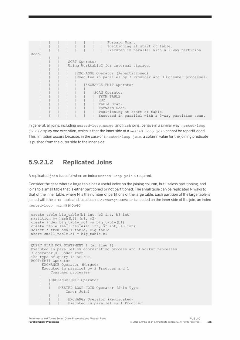
| | | | | | | | Forward Scan. | | | | | | | | Positioning at start of table. | | | | | | | | Executed in parallel with a 2-way partition scan. | | | | | | |SORT Operator | | | |Using Worktable2 for internal storage. | | | | | | | | |EXCHANGE Operator (Repartitioned) | | | | |Executed in parallel by 3 Producer and 3 Consumer processes. | | | | | | | | | | |EXCHANGE:EMIT Operator | | | | | | | | | | | | |SCAN Operator | | | | | | | FROM TABLE | | | | | | | RB2 | | | | | | | Table Scan. | | | | | | | Forward Scan. | | | | | | | Positioning at start of table. | | | | | | | Executed in parallel with a 3-way partition scan.
In general, all joins, including nested-loop, merge, and hash joins, behave in a similar way. nested-loop joins display one exception, which is that the inner side of a nested-loop join cannot be repartitioned. This limitation occurs because, in the case of a nested-loop join, a column value for the joining predicate is pushed from the outer side to the inner side.
5.9.2.1.2 Replicated Joins
A replicated join is useful when an index nested-loop join is required.
Consider the case where a large table has a useful index on the joining column, but useless partitioning, and joins to a small table that is either partitioned or not partitioned. The small table can be replicated N ways to that of the inner table, where N is the number of partitions of the large table. Each partition of the large table is joined with the small table and, because no exchange operator is needed on the inner side of the join, an index nested-loop join is allowed.
create table big_table(b1 int, b2 int, b3 int) partition by hash(b3) (p1, p2)create index big_table_nc1 on big_table(b1)create table small_table(s1 int, s2 int, s3 int)select * from small_table, big_table where small_table.s1 = big_table.b1
QUERY PLAN FOR STATEMENT 1 (at line 1). Executed in parallel by coordinating process and 3 worker processes.7 operator(s) under rootThe type of query is SELECT.ROOT:EMIT Operator |EXCHANGE Operator (Merged) |Executed in parallel by 2 Producer and 1 Consumer processes. | | |EXCHANGE:EMIT Operator | | | | |NESTED LOOP JOIN Operator (Join Type: Inner Join) | | | | | | |EXCHANGE Operator (Replicated) | | | |Executed in parallel by 1 Producer
Performance and Tuning Series: Query Processing and Abstract PlansParallel Query Processing
P U B L I C© 2015 SAP SE or an SAP affiliate company. All rights reserved. 155

and 2 Consumer processes. | | | | | | | | |EXCHANGE:EMIT Operator | | | | | | | | | | |SCAN Operator | | | | | | FROM TABLE | | | | | | small_table | | | | | | Table Scan. | | | | | | |SCAN Operator | | | | FROM TABLE | | | | big_table | | | | Index : big_table_nc1 | | | | Forward Scan. | | | | Positioning by key. | | | | Keys are: | | | | b1 ASC | | | | Executed in parallel with a 2-way hash scan.
5.9.2.1.3 Parallel Reformatting
Parallel reformatting is especially useful when you are working with a nested-loop join. Usually, reformatting refers to materializing the inner side of a nested join into a worktable, then creating an index on the joining predicate.
With parallel queries and nested-loop join, reformatting is also helpful when there is no useful index on the joining column or nested-loop join is the only viable option for a query because of the server/session/query level settings. This is an important option for SAP ASE. The outer side may have useful partitioning and, if not, it can be repartitioned to create that useful partitioning. But for the inner side of a nested-loop join, any repartitioning means that the table must be reformatted into a worktable that uses the new partitioning strategy. The inner scan of a nested-loop join must then access the worktable.
In this next example, partitioning for tables RA2 and RB2 is on columns (a1, a2) and (b1, b2) respectively. The query is run with merge and hash join turned off for the session.
select * from RA2, RB2 where a1 = b1 and a2 = b3
QUERY PLAN FOR STATEMENT 1 (at line 1). Executed in parallel by coordinating process and 12 worker processes.17 operator(s) under rootThe type of query is SELECT.ROOT:EMIT Operator |SEQUENCER Operator has 2 children. | | |EXCHANGE Operator (Merged) | |Executed in parallel by 4 Producer and 1 Consumer processes. | | | | |EXCHANGE:EMIT Operator | | | | | | |STORE Operator | | | | Worktable1 created, in allpages locking mode, for REFORMATTING. | | | | Creating clustered index. | | | | | | | | |INSERT Operator | | | | | The update mode is direct. | | | | | | | | | | |EXCHANGE Operator
156P U B L I C© 2015 SAP SE or an SAP affiliate company. All rights reserved.
Performance and Tuning Series: Query Processing and Abstract PlansParallel Query Processing

(Repartitioned) | | | | | |Executed in parallel by 2 Producer and 4 Consumer processes. | | | | | | | | | | | | |EXCHANGE:EMIT Operator | | | | | | | | | | | | | | |RESTRICT Operator | | | | | | | | | | | | | | | | |SCAN Operator | | | | | | | | | FROM TABLE | | | | | | | | | RB2 | | | | | | | | | Table Scan. | | | | | | | | | Executed in parallel with a 2-way partition scan. | | | | | | | | | | TO TABLE | | | | | Worktable1. | | |EXCHANGE Operator (Merged) | |Executed in parallel by 4 Producer and 1 Consumer processes. | | | | |EXCHANGE:EMIT Operator | | | | | | |NESTED LOOP JOIN Operator (Join Type: Inner Join) | | | | | | | | |EXCHANGE Operator (Repartitioned) | | | | |Executed in parallel by 2 Producer and 4 Consumer processes. | | | | | | | | | | |EXCHANGE:EMIT Operator | | | | | | | | | | | | |RESTRICT Operator | | | | | | | | | | | | | | |SCAN Operator | | | | | | | | FROM TABLE | | | | | | | | RA2 | | | | | | | | Table Scan. | | | | | | | | Executed in parallel with a 2-way partition scan. | | | | |SCAN Operator | | | | | FROM TABLE | | | | | Worktable1. | | | | | Using Clustered Index. | | | | | Forward Scan. | | | | | Positioning by key.
The sequence operator executes all of its child operators but the last, before executing the last child operator. In this case, the sequence operator executes the first child operator, which reformats table RB2 into a worktable using a four-way hash partitioning on columns b1 and b3. The table RA2 is also repartitioned four ways to match the stored partitioning of the worktable.
Performance and Tuning Series: Query Processing and Abstract PlansParallel Query Processing
P U B L I C© 2015 SAP SE or an SAP affiliate company. All rights reserved. 157
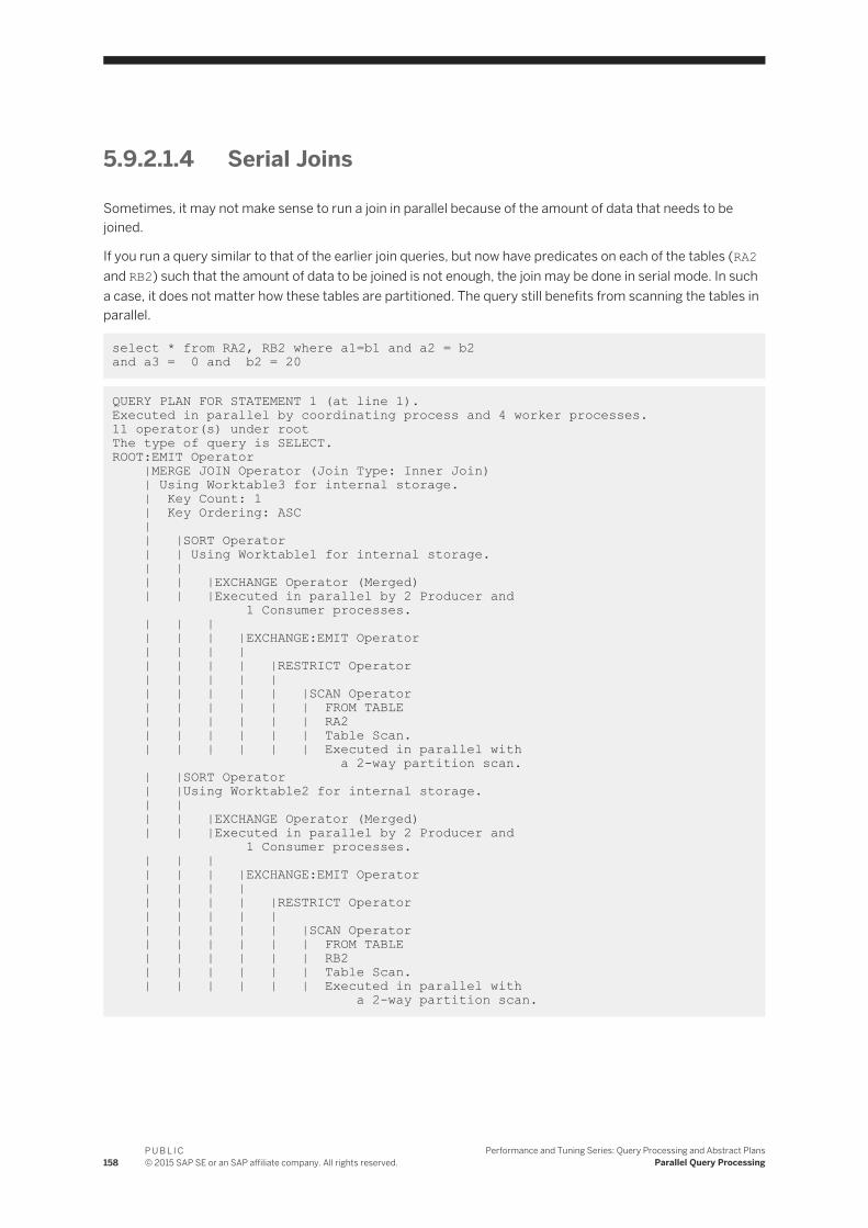
5.9.2.1.4 Serial Joins
Sometimes, it may not make sense to run a join in parallel because of the amount of data that needs to be joined.
If you run a query similar to that of the earlier join queries, but now have predicates on each of the tables (RA2 and RB2) such that the amount of data to be joined is not enough, the join may be done in serial mode. In such a case, it does not matter how these tables are partitioned. The query still benefits from scanning the tables in parallel.
select * from RA2, RB2 where a1=b1 and a2 = b2 and a3 = 0 and b2 = 20
QUERY PLAN FOR STATEMENT 1 (at line 1). Executed in parallel by coordinating process and 4 worker processes.11 operator(s) under rootThe type of query is SELECT.ROOT:EMIT Operator |MERGE JOIN Operator (Join Type: Inner Join) | Using Worktable3 for internal storage. | Key Count: 1 | Key Ordering: ASC | | |SORT Operator | | Using Worktable1 for internal storage. | | | | |EXCHANGE Operator (Merged) | | |Executed in parallel by 2 Producer and 1 Consumer processes. | | | | | | |EXCHANGE:EMIT Operator | | | | | | | | |RESTRICT Operator | | | | | | | | | | |SCAN Operator | | | | | | FROM TABLE | | | | | | RA2 | | | | | | Table Scan. | | | | | | Executed in parallel with a 2-way partition scan. | |SORT Operator | |Using Worktable2 for internal storage. | | | | |EXCHANGE Operator (Merged) | | |Executed in parallel by 2 Producer and 1 Consumer processes. | | | | | | |EXCHANGE:EMIT Operator | | | | | | | | |RESTRICT Operator | | | | | | | | | | |SCAN Operator | | | | | | FROM TABLE | | | | | | RB2 | | | | | | Table Scan. | | | | | | Executed in parallel with a 2-way partition scan.
158P U B L I C© 2015 SAP SE or an SAP affiliate company. All rights reserved.
Performance and Tuning Series: Query Processing and Abstract PlansParallel Query Processing

5.9.2.1.5 Semijoins
Semijoins, which result from flattening of in/exist subqueries, behave the same way as regular inner joins.
However, replicated joins are not used for semijoins, because an outer row can match more than one time in such a situation.
5.9.2.1.6 Outer Joins
In terms of parallel processing for outer joins, replicated joins are not considered. Everything else behaves in a similar way as regular inner joins.
One other point of difference is that no partition elimination is done for any table in an outer join that belongs to the outer group.
5.9.2.1.7 Vector Aggregation
Vector aggregation refers to queries with group-bys. There are different ways SAP ASE can perform vector aggregation. The actual algorithms are not described here; only the technique for parallel evaluation is shown in the following sections.
In-Partitioned Vector Aggregation
If any base or intermediate relation requires a grouping and is partitioned on a subset, or the same columns as that of the columns in the group by clause, the grouping operation can be done in parallel on each of the partitions and the resultant grouped streams merged using a simple N-to-1 exchange.
This is because a given group cannot appear in more than one stream. The same restriction applies to grouping over any SQL query as long as you use semantics-based partitioning on the grouping columns or a subset of them. This method of parallel vector aggregation is called in-partitioned aggregation.
The following query uses a parallel in-partitioned vector aggregation since range partitioning is defined on the columns a1 and a2, which also happens to be the columns on which the aggregation is needed.
select count(*), a1, a2 from RA2 group by a1,a2
QUERY PLAN FOR STATEMENT 1 (at line 1). Executed in parallel by coordinating process and 2 worker processes.4 operator(s) under rootThe type of query is SELECT.ROOT:EMIT Operator |EXCHANGE Operator (Merged) |Executed in parallel by 2 Producer and 1 Consumer processes. | | |EXCHANGE:EMIT Operator
Performance and Tuning Series: Query Processing and Abstract PlansParallel Query Processing
P U B L I C© 2015 SAP SE or an SAP affiliate company. All rights reserved. 159

| | | | |HASH VECTOR AGGREGATE Operator | | | GROUP BY | | | Evaluate Grouped COUNT AGGREGATE. | | | Using Worktable1 for internal storage. | | | | | | |SCAN Operator | | | | FROM TABLE | | | | RA2 | | | | Table Scan. | | | | Forward Scan. | | | | Positioning at start of table. | | | | Executed in parallel with a 2-way partition scan. | | | | Using I/O Size 2 Kbytes for data pages. | | | | With LRU Buffer Replacement Strategy for data pages.
Repartitioned Vector Aggregation
Sometimes, the partitioning of the table or the intermediate results may not be useful for the grouping operation.
It may still be worthwhile to do the grouping operation in parallel by repartitioning the source data to match the grouping columns, then applying the parallel vector aggregation. Such a scenario is shown below, where the partitioning is on columns (a1, a2), but the query requires a vector aggregation on column a1.
select count(*), a1 from RA2 group by a1 QUERY PLAN FOR STATEMENT 1 (at line 1).Executed in parallel by coordinating process and 4 worker processes.6 operator(s) under rootThe type of query is SELECT.ROOT:EMIT Operator |EXCHANGE Operator (Merged) |Executed in parallel by 2 Producer and 1 Consumer processes. | | |EXCHANGE:EMIT Operator | | | | |HASH VECTOR AGGREGATE Operator | | | GROUP BY | | | Evaluate Grouped COUNT AGGREGATE. | | | Using Worktable1 for internal storage. | | | | | | |EXCHANGE Operator (Repartitioned) | | | |Executed in parallel by 2 Producer and 2 Consumer processes. | | | | | | | | |EXCHANGE:EMIT Operator | | | | | | | | | | |SCAN Operator | | | | | | FROM TABLE | | | | | | RA2 | | | | | | Table Scan. | | | | | | Forward Scan. | | | | | | Positioning at start of table. | | | | | | Executed in parallel with a 2-way partition scan.
160P U B L I C© 2015 SAP SE or an SAP affiliate company. All rights reserved.
Performance and Tuning Series: Query Processing and Abstract PlansParallel Query Processing

Two-Phased Vector Aggregation
For the query in the previous example, repartitioning may be expensive. Another possibility is to do a first level of grouping, merge the data using a N-to-1 exchange operator, then do another level of grouping. This is called a two-phased vector aggregation.
Depending on the number of duplicates for the grouping column, SAP ASE can reduce the cardinality of the data streaming through the N-to-1 exchange, which reduces the cost of the second level of grouping.
select count(*), a1 from RA2 group by a1 QUERY PLAN FOR STATEMENT 1 (at line 1).Executed in parallel by coordinating process and 2 worker processes.5 operator(s) under rootThe type of query is SELECT.ROOT:EMIT Operator |HASH VECTOR AGGREGATE Operator | GROUP BY | Evaluate Grouped SUM OR AVERAGE AGGREGATE. | Using Worktable2 for internal storage. | | |EXCHANGE Operator (Merged) | |Executed in parallel by 2 Producer and 1 Consumer processes. | | | | |EXCHANGE:EMIT Operator | | | | | | |HASH VECTOR AGGREGATE Operator | | | | GROUP BY | | | | Evaluate Grouped COUNT AGGREGATE. | | | | Using Worktable1 for internal storage. | | | | | | | | |SCAN Operator | | | | | FROM TABLE | | | | | RA2 | | | | | Table Scan. | | | | | Executed in parallel with a 2-way partition scan.
Serial Vector Aggregation
As with some of the earlier examples, if the amount of data flowing into the grouping operator is restricted by using a predicate, executing that query in parallel may not make much sense. In such a case, the partitions are scanned in parallel and an N-to-1 exchange operator is used to serialize the stream followed by a serial vector aggregation.
select count(*), a1, a2 from RA2 where a1 between 100 and 200group by a1, a2QUERY PLAN FOR STATEMENT 1 (at line 1).Executed in parallel by coordinating process and 2 worker processes.4 operator(s) under rootThe type of query is SELECT.ROOT:EMIT Operator |HASH VECTOR AGGREGATE Operator | GROUP BY | Evaluate Grouped COUNT AGGREGATE.
Performance and Tuning Series: Query Processing and Abstract PlansParallel Query Processing
P U B L I C© 2015 SAP SE or an SAP affiliate company. All rights reserved. 161

| Using Worktable1 for internal storage. | | |EXCHANGE Operator (Merged) | |Executed in parallel by 2 Producer and 1 Consumer processes. | | | | |EXCHANGE:EMIT Operator | | | | | | |SCAN Operator | | | | FROM TABLE | | | | RA2 | | | | Positioning at start of table. | | | | Executed in parallel with a 2-way partition scan.
You cannot always group on the partitioning columns, or take advantage of a table that is already partitioned on the grouping columns. The query optimizer determines if it is better to repartition and perform the grouping in parallel, or merge the data stream in a partitioned table and do the grouping in serial or a two-phased aggregation.
5.9.2.1.8 distinct
Queries with distinct operations are the same as grouped vector aggregation without the aggregation part.
For example:
select distinct a1, a2 from RA2
is same as:
select a1, a2 from RA2 group by a1, a2
All of the methodologies that are applicable to vector aggregates are applicable here as well.
5.9.2.1.9 Queries with an in List
SAP ASE uses an optimized technique to handle an in list, which is a common SQL construct.
So, a construct like:
col in (value1, value2,..valuek)
is same as:
col = value1 OR col = value2 OR .... col = valuek
The values in the in list are put into a special in-memory table and sorted for removal of duplicates.The table is then joined back with the base table using an index nested-loop join. The following example illustrates this with two values in the in list that correspond to two values in the or list:
select * from RA2 where a3 in (1425, 2940) QUERY PLAN FOR STATEMENT 1 (at line 1).
162P U B L I C© 2015 SAP SE or an SAP affiliate company. All rights reserved.
Performance and Tuning Series: Query Processing and Abstract PlansParallel Query Processing

Executed in parallel by coordinating process and 2 worker processes.6 operator(s) under rootThe type of query is SELECT.ROOT:EMIT Operator |EXCHANGE Operator (Merged) |Executed in parallel by 2 Producer and 1 Consumer processes. | | |EXCHANGE:EMIT Operator | | | | |NESTED LOOP JOIN Operator (Join Type: Inner Join) | | | | | | |SCAN Operator | | | | FROM OR List | | | | OR List has up to 2 rows of OR/IN values. | | | | | | |RESTRICT Operator | | | | | | | | |SCAN Operator | | | | | FROM TABLE | | | | | RA2 | | | | | Index : RA2_NC1 | | | | | Forward Scan. | | | | | Positioning by key. | | | | | Keys are: | | | | | a3 ASC | | | | | Executed in parallel with a 2-way hash scan.
5.9.2.1.10 Queries with or Clauses
SAP ASE takes a disjunctive predicate like an or clause and applies each side of the disjunction separately to qualify a set of row IDs (RIDs).
The set of conjunctive predicates on each side of the disjunction must be indexable. Also, the conjunctive predicates on each side of the disjunction cannot have further disjunction within them; that is, it makes little sense to use an arbitrarily deep nesting of disjunctive and conjunctive clauses. In the next example, a disjunctive predicate is taken on the same column (you can have predicates on different columns as long as you have indexes that can do inexpensive scans), but the predicates may qualify an overlapping set of data rows. SAP ASE uses the predicates on each side of the disjunction separately and qualifies a set of row IDs. These row IDs are then subjected to duplicate elimination.
select a3 from RA2 where a3 = 2955 or a3 > 2990 QUERY PLAN FOR STATEMENT 1 (at line 1).Executed in parallel by coordinating process and 2 worker processes.8 operator(s) under rootThe type of query is SELECT.ROOT:EMIT Operator |EXCHANGE Operator (Merged) |Executed in parallel by 2 Producer and 1 Consumer processes. | | |EXCHANGE:EMIT Operator | | | | |RID JOIN Operator | | | Using Worktable2 for internal storage. | | |
Performance and Tuning Series: Query Processing and Abstract PlansParallel Query Processing
P U B L I C© 2015 SAP SE or an SAP affiliate company. All rights reserved. 163

| | | |HASH UNION Operator has 2 children. | | | | Using Worktable1 for internal storage. | | | | | | | | |SCAN Operator | | | | | FROM TABLE | | | | | RA2 | | | | | Index : RA2_NC1 | | | | | Forward Scan. | | | | | Positioning by key. | | | | | Index contains all needed columns.Base table will not be read. | | | | | Keys are: | | | | | a3 ASC | | | | | Executed in parallel with a 2-way hash scan. | | | | | | | | |SCAN Operator | | | | | FROM TABLE | | | | | RA2 | | | | | Index : RA2_NC1 | | | | | Forward Scan. | | | | | Positioning by key. | | | | | Index contains all needed columns. Base table will not be read. | | | | | Keys are: | | | | | a3 ASC | | | | | Executed in parallel with a 2-way hash scan. | | | |RESTRICT Operator | | | | | | | | |SCAN Operator | | | | | FROM TABLE | | | | | RA2 | | | | | Using Dynamic Index. | | | | | Forward Scan. | | | | | Positioning by Row IDentifier (RID.) | | | | | Using I/O Size 2 Kbytes for data pages. | | | | | With LRU Buffer Replacement Strategy for data pages.
Two separate index scans are employed using the index RA2_NC1, which is defined on the column a3. The qualified set of row IDs are then checked for duplicate row IDs, and finally, joined back to the base table. Note the line Positioning by Row Identifier (RID). You can use different indexes for each side of the disjunction, depending on what the predicates are, as long as they are indexable. One way to easily identify this is to run the query separately with each side of the disjunction to make sure that the predicates are indexable. SAP ASE may not choose an index intersection if it seems more expensive than a single scan of the table.
5.9.2.1.11 Queries with an order by Clause
If a query requires sorted output because of the presence of an order by clause, the sort can be applied in parallel.
The sort is avoided if there is some inherent ordering available. If SAP ASE is forced to do the sort, it sees if the sort can be done in parallel. To do that, SAP ASE may repartition an existing data stream or it may use the
164P U B L I C© 2015 SAP SE or an SAP affiliate company. All rights reserved.
Performance and Tuning Series: Query Processing and Abstract PlansParallel Query Processing

existing partitioning scheme, then apply the sort to each of the constituent streams. The resultant data is merged using an N-to-1 order, preserving the exchange operator.
select * from RA2 order by a1, a2 QUERY PLAN FOR STATEMENT 1 (at line 1).Executed in parallel by coordinating process and 2 worker processes.4 operator(s) under rootThe type of query is SELECT.ROOT:EMIT Operator |EXCHANGE Operator (Merged) |Executed in parallel by 2 Producer and 1 Consumer processes. | | |EXCHANGE:EMIT Operator | | | | |SORT Operator | | | Using Worktable1 for internal storage. | | | | | | |SCAN Operator | | | | FROM TABLE | | | | RA2 | | | | Index : RA2_NC2L | | | | Forward Scan. | | | | Positioning at index start. | | | | Executed in parallel with a 2-way partition scan.
Depending upon the volume of data to be sorted, and the available resources, SAP ASE may repartition the data stream to a higher degree than the current degree of the stream, so that the sort operation is faster. The degrees of sorting depends on whether the benefit obtained from doing the sort in parallel far outweighs the overheads of repartitioning.
5.9.2.2 Scalar Aggregation
The Transact-SQL scalar aggregation operation can be done in serial or in parallel.
Two-Phased Scalar Aggregation
In a parallel scalar aggregation, the aggregation operation is performed in two phases, using two scalar aggregate operators.
In the first phase, the lower scalar aggregation operator performs aggregation on the data stream. The result of scalar aggregation from the first phase is merged using a many-to-one exchange operator, and this stream is aggregated a second time.
In case of a count(*) aggregation, the second phase aggregation performs a scalar sum. This is highlighted in the showplan output of the next example.
select count(*) from RA2
QUERY PLAN FOR STATEMENT 1 (at line 1). Executed in parallel by coordinating process and 2 worker processes.5 operator(s) under root
Performance and Tuning Series: Query Processing and Abstract PlansParallel Query Processing
P U B L I C© 2015 SAP SE or an SAP affiliate company. All rights reserved. 165

The type of query is SELECT.ROOT:EMIT Operator |SCALAR AGGREGATE Operator | Evaluate Ungrouped SUM OR AVERAGE AGGREGATE. | | |EXCHANGE Operator (Merged) | |Executed in parallel by 2 Producer and 1 Consumer processes. | | | | |EXCHANGE:EMIT Operator | | | | | | |SCALAR AGGREGATE Operator | | | | Evaluate Ungrouped COUNT AGGREGATE. | | | | | | | | |SCAN Operator | | | | | FROM TABLE | | | | | RA2 | | | | | Table Scan. | | | | | Forward Scan. | | | | | Positioning at start of table. | | | | | Executed in parallel with a 2-way partition scan. | | | | | Using I/O Size 2 Kbytes for data pages. | | | | | With LRU Buffer Replacement Strategy for data pages.
Serial Aggregation
If the amount of data to be aggregated is not enough to guarantee a performance advantage, a serial aggregation may be the preferred technique. In case of a serial aggregation, the result of the scan is merged using a many-to-one exchange operator.
This is shown in the example below, where a selective predicate has been added to minimize the amount of data flowing into the scalar aggregate operator. In such a case, it probably does not make sense to do the aggregation in parallel.
select count(*) from RA2 where a2 = 10
QUERY PLAN FOR STATEMENT 1 (at line 1). Executed in parallel by coordinating process and 2 worker processes.4 operator(s) under rootThe type of query is SELECT.ROOT:EMIT Operator |SCALAR AGGREGATE Operator | Evaluate Ungrouped COUNT AGGREGATE. | | |EXCHANGE Operator (Merged) | |Executed in parallel by 2 Producer and 1 Consumer processes. | | | | |EXCHANGE:EMIT Operator | | | | | | |SCAN Operator | | | | FROM TABLE | | | | RA2 | | | | Table Scan. | | | | Forward Scan.
166P U B L I C© 2015 SAP SE or an SAP affiliate company. All rights reserved.
Performance and Tuning Series: Query Processing and Abstract PlansParallel Query Processing

| | | | Positioning at start of table. | | | | Executed in parallel with a 2-way partition scan. | | | | Using I/O Size 2 Kbytes for data pages. | | | | With LRU Buffer Replacement Strategy for data pages.
5.9.2.3 union all Operator
union all operators are implemented using a physical operator by the same name. union all is a fairly simple operation and should be used in parallel only when a query is moving large amounts of data.
Parallel union all
The only condition to generating a parallel union all is that each of its operands must be of the same degree, irrespective of the type of partitioning they have.
The following example (using table HA2) shows a union all operator being processed in parallel. The position of the exchange operator above the union all operator signifies that it is being processed by multiple threads:
create table HA2(a1 int, a2 int, a3 int) partition by hash(a1, a2) (p1, p2)select * from RA2union allselect * from HA2QUERY PLAN FOR STATEMENT 1 (at line 1).Executed in parallel by coordinating process and 2 worker processes.The type of query is SELECT.ROOT:EMIT Operator |EXCHANGE Operator (Merged) |Executed in parallel by 2 Producer and 1 Consumer processes. | | |EXCHANGE:EMIT Operator | | | | |UNION ALL Operator has 2 children. | | | | | | |SCAN Operator | | | | FROM TABLE | | | | RA2 | | | | Table Scan.. . . . . . . . . . . . . . . . . . . | | | | Executed in parallel with a 2-way partition scan.. . . . . . . . . . . . . . . . . . . | | | | | | |SCAN Operator | | | | FROM TABLE | | | | HA2 | | | | Table Scan. . . . . . . . . . . . . . . . . . . . | | | | Executed in parallel with a 2-way partition scan.
Performance and Tuning Series: Query Processing and Abstract PlansParallel Query Processing
P U B L I C© 2015 SAP SE or an SAP affiliate company. All rights reserved. 167

Serial union all
In the next example, the data from each side of the union operator is restricted by selective predicates on either side.
The amount of data being sent through the union all operator is small enough that decides not to run the unions in parallel. Instead, each scan of the tables RA2 and HA2 are organized by putting 2-to-1 exchange operators on each side of the union. The resultant operands are then processed in parallel by the union all operator:
select * from RA2 where a2 > 2400union allselect * from HA2 where a3 in (10,20)
Executed in parallel by coordinating process and 4 worker processes. 7 operator(s) under rootThe type of query is SELECT. ROOT:EMIT Operator |UNION ALL Operator has 2 children. | | |EXCHANGE Operator (Merged) | |Executed in parallel by 2 Producer and 1 Consumer processes. | | | | |EXCHANGE:EMIT Operator | | | | | | |SCAN Operator | | | | FROM TABLE | | | | RA2 | | | | Table Scan. | | | | Executed in parallel with a 2-way partition scan. | | |EXCHANGE Operator (Merged) | |Executed in parallel by 2 Producer and 1 Consumer processes. | | | | |EXCHANGE:EMIT Operator | | | | | | |SCAN Operator | | | | FROM TABLE | | | | HA2 | | | | Table Scan. | | | | Executed in parallel with a 2-way partition scan.
168P U B L I C© 2015 SAP SE or an SAP affiliate company. All rights reserved.
Performance and Tuning Series: Query Processing and Abstract PlansParallel Query Processing

5.9.2.4 Parallelism of Attribute-Sensitive Operation
Attribute-sensitive operations include joins, vector aggregations, and unions.
5.9.2.5 Subqueries
There are different methods that can reduce the cost of processing subqueries.
Parallel optimization depends on the type of subquery:
● Materialized subqueries – parallel query methods are not considered for the materialization step.● Flattened subqueries – parallel query optimization is considered only when the subquery is flattened to a
regular inner join or a semijoin.● Nested subqueries – parallel operations are considered for the outermost query block in a query
containing a subquery; the inner, nested queries always execute serially. This means that all tables in nested subqueries are accessed serially. In the following example, the table RA2 is accessed in parallel, but the result is that the table is serialized using a two-to-one exchange operator before accessing the subquery. The table RB2 inside the subquery is accessed in serial.
select count(*) from RA2 where not exists (select * from RB2 where RA2.a1 = b1)QUERY PLAN FOR STATEMENT 1 (at line 1).Executed in parallel by coordinating process and 2 worker processes.8 operator(s) under rootThe type of query is SELECT.ROOT:EMIT Operator |SCALAR AGGREGATE Operator | Evaluate Ungrouped COUNT AGGREGATE. | | |SQFILTER Operator has 2 children. | | | | |EXCHANGE Operator (Merged) | | |Executed in parallel by 2 Producer and 1 Consumer processes. | | | | | | |EXCHANGE:EMIT Operator | | | | | | | | |RESTRICT Operator | | | | | | | | | | |SCAN Operator | | | | | | FROM TABLE | | | | | | RA2 | | | | | | Index : RA2_NC2L | | | | | | Forward Scan. | | | | | | Executed in parallel with a 2-way partition scan. | | | | Run subquery 1 (at nesting level 1). | |
| | QUERY PLAN FOR SUBQUERY 1 (at nesting level 1 and at line 2). | | | | Correlated Subquery. | | Subquery under an EXISTS predicate. | | | | |SCALAR AGGREGATE Operator | | | Evaluate Ungrouped ANY AGGREGATE. | | | Scanning only up to the first qualifying row. | | |
Performance and Tuning Series: Query Processing and Abstract PlansParallel Query Processing
P U B L I C© 2015 SAP SE or an SAP affiliate company. All rights reserved. 169

| | | |SCAN Operator | | | | FROM TABLE | | | | RB2 | | | | Table Scan. | | | | Forward Scan. | | | | END OF QUERY PLAN FOR SUBQUERY 1.
The following example shows an in subquery flattened into a semijoin. SAP ASE converts this into an inner join to provide greater flexibility in shuffling the tables in the join order. As seen below, the table RB2, which was originally in the subquery, is now being accessed in parallel.
select * from RA2 where a1 in (select b1 from RB2) QUERY PLAN FOR STATEMENT 1 (at line 1).Executed in parallel by coordinating process and 5 worker processes.10 operator(s) under rootThe type of query is SELECT.ROOT:EMIT Operator |EXCHANGE Operator (Merged) |Executed in parallel by 3 Producer and 1 Consumer processes. | | |EXCHANGE:EMIT Operator | | | | |MERGE JOIN Operator (Join Type: Inner Join) | | | Using Worktable3 for internal storage. | | | Key Count: 1 | | | Key Ordering: ASC | | | | | | |SORT Operator | | | | Using Worktable1 for internal storage. | | | | | | | | |SCAN Operator | | | | | FROM TABLE | | | | | RB2 | | | | | Table Scan. | | | | | Executed in parallel with a 3-way partition scan. | | | | | | |SORT Operator | | | | Using Worktable2 for internal storage. | | | | | | | | |EXCHANGE Operator (Merged) | | | | |Executed in parallel by 2 Producer and 3 Consumer processes. | | | | | | | | | | |EXCHANGE:EMIT Operator | | | | | | | | | | | | |RESTRICT Operator | | | | | | | | | | | | | | |SCAN Operator | | | | | | | | FROM TABLE | | | | | | | | RA2 | | | | | | | | Index : RA2_NC2L | | | | | | | | Forward Scan. | | | | | | | | Positioning at index start. | | | | | | | | Executed in parallel with a 2-way partition scan.
170P U B L I C© 2015 SAP SE or an SAP affiliate company. All rights reserved.
Performance and Tuning Series: Query Processing and Abstract PlansParallel Query Processing

5.9.2.6 select into Clauses
Queries with select into clauses create a new table in which to store the query’s result set.
SAP ASE optimizes the base query portion of a select into command in the same way it does a standard query, considering both parallel and serial access methods. A select into statement that is executed in parallel:
● Creates the new table using the columns specified in the select into statement.● Creates N partitions in the new table, where N is the degree of parallelism that the optimizer chooses for
the insert operation in the query.● Populates the new table with query results, using N worker processes.● Unpartitions the new table, if no specific destination partitioning is required.
Performing a select into statement in parallel requires more steps than an equivalent serial query plan. This is a simple select into done in parallel:
select * into RAT2 from RA2 QUERY PLAN FOR STATEMENT 1 (at line 1).Executed in parallel by coordinating process and 2 worker processes.4 operator(s) under rootThe type of query is INSERT.ROOT:EMIT Operator |EXCHANGE Operator (Merged) |Executed in parallel by 2 Producer and 1 Consumer processes. | | |EXCHANGE:EMIT Operator | | | | |INSERT Operator | | | The update mode is direct. | | | | | | |SCAN Operator | | | | FROM TABLE | | | | RA2 | | | | Table Scan. | | | | Forward Scan. | | | | Positioning at start of table. | | | | Executed in parallel with a 2-way partition scan. | | | | | | TO TABLE | | | RAT2 | | | Using I/O Size 2 Kbytes for data pages.
SAP ASE does not try to increase the degree of the stream coming from the scan of table RA2, and uses it to do a parallel insert into the destination table. The destination table is initially created using round-robin partitioning of degree two. After the insert, the table is unpartitioned.
If the data set to be inserted is not big enough, SAP ASE may choose to insert this data in serial. The scan of the source table can still be done in parallel. The destination table is then created as an unpartitioned table.
The select into allows destination partitioning to be specified. In such a case, the destination table is created using that partitioning, and SAP ASE finds the most optimal way to insert data. If the destination table must be partitioned the same way as the source data, and there is enough data to insert, the insert operator executes in parallel.
Performance and Tuning Series: Query Processing and Abstract PlansParallel Query Processing
P U B L I C© 2015 SAP SE or an SAP affiliate company. All rights reserved. 171

The next example shows the same partitioning for source and destination table, and demonstrates that SAP ASE recognizes this scenario and chooses not to repartition the source data.
select * into new_table partition by range(a1, a2)(p1 values <= (500,100), p2 values <= (1000, 2000)) from RA2QUERY PLAN FOR STATEMENT 1 (at line 1).Executed in parallel by coordinating process and 2 worker processes.4 operator(s) under rootThe type of query is INSERT.ROOT:EMIT Operator |EXCHANGE Operator (Merged) |Executed in parallel by 2 Producer and 1 Consumer processes. | | |EXCHANGE:EMIT Operator | | | | |INSERT Operator | | | The update mode is direct. | | | | | | |SCAN Operator | | | | FROM TABLE | | | | RA2 | | | | Table Scan. | | | | Forward Scan. | | | | Positioning at start of table. | | | | Executed in parallel with a 2-way partition scan. | | | | | | TO TABLE | | | RRA2 | | | Using I/O Size 16 Kbytes for data pages.
If the source partitioning does not match that of the destination table, the source data must be repartitioned. This is illustrated in the next example, where the insert is done in parallel using two worker processes after the data is repartitioned using a 2-to-2 exchange operator that converts the data from range partitioning to hash partitioning.
select * into HHA2 partition by hash(a1, a2)(p1, p2)from RA2QUERY PLAN FOR STATEMENT 1 (at line 1).Executed in parallel by coordinating process and 4 worker processes.6 operator(s) under rootThe type of query is INSERT.ROOT:EMIT Operator|EXCHANGE Operator (Merged)|Executed in parallel by 2 Producer and 1 Consumer processes.|| |EXCHANGE:EMIT Operator| || | |INSERT Operator| | | The update mode is direct.| | || | | |EXCHANGE OperatorEXCHANGE Operator ( Merged)| | | |Executed in parallel by 2 Producer and 2 Consumer processes.| | | || | | | |EXCHANGE:EMIT Operator| | | | || | | | | |SCAN Operator
172P U B L I C© 2015 SAP SE or an SAP affiliate company. All rights reserved.
Performance and Tuning Series: Query Processing and Abstract PlansParallel Query Processing

| | | | | | FROM TABLE| | | | | | RA2| | | | | | Table Scan.| | | | | | Forward Scan.| | | | | | Positioning at start of table.| | | | | | Executed in parallel with a 2-way partition scan.| | || | | TO TABLE| | | HHA2| | | Using I/O Size 16 Kbytes for data pages.
5.9.2.7 insert/delete/update Operations
insert, delete, and update operations are performed in serial.
However, tables other than the destination table used in the query to qualify rows to be deleted or updated, can be accessed in parallel.
delete from RA2 where exists(select * from RB2 where RA2.a1 = b1 and RA2.a2 = b2)QUERY PLAN FOR STATEMENT 1 (at line 1).Executed in parallel by coordinating process and 3 worker processes.9 operator(s) under rootThe type of query is DELETE.ROOT:EMIT Operator|DELETE Operator| The update mode is deferred.|| |NESTED LOOP JOIN Operator (Join Type: Inner Join)| || | |SORT Operator| | | Using Worktable1 for internal storage.| | || | | |EXCHANGE Operator (Merged)| | | |Executed in parallel by 3 Producer and 1 Consumer processes.| | | || | | | |EXCHANGE:EMIT Operator| | | | || | | | | |RESTRICT Operator| | | | | || | | | | | |SCAN Operator| | | | | | | FROM TABLE| | | | | | | RB2| | | | | | | Table Scan.| | | | | | | Forward Scan.| | | | | | | Positioning at start of table.| | | | | | | Executed in parallel with a 3-way partition scan.| | | | | | | Using I/O Size 2 Kbytes for data pages.| | | | | | | With LRU Buffer Replacement Strategy for data pages.| || | |RESTRICT Operator| | || | | |SCAN Operator
Performance and Tuning Series: Query Processing and Abstract PlansParallel Query Processing
P U B L I C© 2015 SAP SE or an SAP affiliate company. All rights reserved. 173

| | | | FROM TABLE| | | | RA2| | | | Index : RA2_NC1| | | | Forward Scan.| | | | Positioning by key.| | | | Keys are:| | | | a3 ASC|| TO TABLE| RA2 | Using I/O Size 2 Kbytes for data pages.
The table RA2, which is being deleted, is scanned and deleted in serial. However, table RB2 was scanned in parallel. The same scenario is true for update or insert statements.
5.9.3 Partition Elimination
One advantage of semantic partitioning is that the query processor may be able to take advantage of this and be able to disqualify range, hash, and list partitions at compile time.
With hash partitions, only equality predicates can be used, whereas for range and list partitions, equality and in-equality predicates can be used to eliminate partitions. For example, consider table RA2 with its semantic partitioning defined on columns a1, a2 where (p1 values <= (500,100) and p2 values <= (1000, 2000)). If there are predicates on columns a1 or columns a1, a2, then it would be possible to do some partition elimination. For example, this statement does not qualify any data:
select * from RA2 where a1 > 1500
You can see this in the showplan output.
QUERY PLAN FOR STATEMENT 1 (at line 1). ................................| | |SCAN Operator| | | FROM TABLE| | | RA2| | | [ Eliminated Partitions : 1 2 ] | | | Index : RA2_NC2L
The phrase Eliminated Partitions identifies the partition in accordance with how it was created and assigns an ordinal number for identification. For table RA2, the partition represented by p1 where (a1, a2) <= (500, 100) is considered to be partition number one and p2 where (a1, a2) > (500, 100) and <= (1000, 2000) is identified as partition number two.
Consider an equality query on a hash-partitioned table where all keys in the hash partitioning have an equality clause. This can be shown by taking table HA2, which is hash-partitioned two ways on columns (a1, a2). The ordinal numbers refer to the order in which partitions are listed in the output of sp_help.
select * from HA2 where a1 = 10 and a2 = 20 QUERY PLAN FOR STATEMENT 1 (at line 1).................................|SCAN Operator| FROM TABLE| HA2| [ Eliminated Partitions : 1 ] | Table Scan.
174P U B L I C© 2015 SAP SE or an SAP affiliate company. All rights reserved.
Performance and Tuning Series: Query Processing and Abstract PlansParallel Query Processing

5.9.4 Partition Skew
Partition skew plays an important part in determining whether a parallel partitioned scan can be used.
Partition skew is defined as the ratio of the size of the largest partition to the average size of a partition. Consider a table with four partitions of sizes 20, 20, 35, and 80 pages. The size of the average partition is (20 + 20 + 35 + 85)/4 = 40 pages. The biggest partition has 85 pages so partition skew is calculated as 85/40 = 2.125. In partitioned scans, the cost of doing a parallel scan is as expensive as doing the scan on the largest partition. Instead, a hash-based partition may turn out to be fast, as each worker process may hash on a page number or an allocation unit and scan its portion of the data. The penalty paid in terms of loss of performance by skewed partitions is not always at the scan level, but rather as more complex operators like several join operations are built over the data. The margin of error increases exponentially in such cases.
Run sp_help on a table to see the partition skews:
sp_help HA2 ........name type partition_type partitions partition_keys ------ -------------------- -------------- -----------HA2 base table hash 2 a1, a2 partition_name partition_id pages segment create_date -------------------------- ------------ ----------- ---------------------------------------- HA2_752002679 752002679 324 default Aug 10 2005 2:05PM HA2_768002736 768002736 343 default Aug 10 2005 2:05PM Partition_Conditions -------------------- NULL Avg_pages Max_pages Min_pages Ratio(Max/Avg) Ratio(Min/Avg) ----------- ----------- ----------- ------------------------------------------------------ 333 343 324 1.030030 0.972973
Alternatively, you can calculate skew by querying the systabstats system catalog, where the number of pages in each partition is listed.
5.9.5 Why Queries Do Not Run in Parallel
SAP ASE does not always run queries in parallel.
Queries are run in serial when:
● There is not enough data to benefit from parallel access.● The query contains no equijoin predicates like:
select * from RA2, RB2 where a1 > b1
● There are not enough resources, such as thread or memory, to run a query in parallel.● Uses a covered scan of a global nonclustered index.
Performance and Tuning Series: Query Processing and Abstract PlansParallel Query Processing
P U B L I C© 2015 SAP SE or an SAP affiliate company. All rights reserved. 175

● Tables and indexes are accessed inside a nested subquery that cannot be flattened.
5.9.6 Runtime Adjustments
If there are not enough worker processes available at runtime, the execution engine attempts to reduce the number of worker processes used by the exchange operators present in the plan.
● First, by attempting to reduce the worker process usage of certain exchange operators in the query plan without resorting to serial recompilation of the query. Depending on the semantics of the query plan, certain exchange operators are adjustable and some are not. Some are limited in the way they can be adjusted.
● Parallel query plans need a minimum number of worker processes to run. When enough worker processes are not available, the query is recompiled serially. When recompilation is impossible, the query is aborted and the appropriate error message is generated.
It does so in two ways:
SAP ASE supports serial recompilation for all:
● Ad hoc select queries, except select into, alter table, and execute immediate queries.● Stored procedures, except select into and alter table queries.
5.9.7 Recognizing and Managing Runtime Adjustments
SAP ASE provides mechanisms to help you observe runtime adjustments of query plans.
● set process_limit_action allows you to abort batches or procedures when runtime adjustments take place.
● showplan prints an adjusted query plan when runtime adjustments occur, and showplan is in effect.
Using set process_limit_action
Use process_limit_action with the set command to monitor the use of adjusted query plans at a session or stored procedure level.
When you set process_limit_action to “abort,” SAP ASE records error 11015 and aborts the query, if an adjusted query plan is required. When you set process_limit_action to “warning,” SAP ASE records error 11014 but still executes the query. For example, this command aborts the batch when a query is adjusted at runtime:
set process_limit_action abort
176P U B L I C© 2015 SAP SE or an SAP affiliate company. All rights reserved.
Performance and Tuning Series: Query Processing and Abstract PlansParallel Query Processing

By examining the occurrences of errors 11014 and 11015 in the error log, you can determine the degree to which SAP ASE uses adjusted query plans instead of optimized query plans. To remove the restriction and allow runtime adjustments, use:
set process_limit_action quiet
See set in the Reference Manual: Commands.
Using showplan
When you use showplan, the optimized plan for a given query is displayed before it runs the query.
When the query plan involves parallel processing, and a runtime adjustment is made, showplan displays this message, followed by the adjusted query plan:
AN ADJUSTED QUERY PLAN IS BEING USED FOR STATEMENT 1 BECAUSE NOT ENOUGH WORKER PROCESSES ARE CURRENTLY AVAILABLE. ADJUSTED QUERY PLAN:
When using set notexec, SAP ASE does not attempt to execute a query, so runtime plans are never displayed.
Reducing the Likelihood of Runtime Adjustments
To reduce the number of runtime adjustments, increase the number of worker processes that are available to parallel queries.
You can do this either by adding more total worker processes to the system or by restricting or eliminating parallel execution for noncritical queries, using either:
● set parallel_degree to set session-level limits on the degree of parallelism, or● The query-level parallel 1 and parallel N clauses to limit the worker process usage of individual
statements.
To reduce the number of runtime adjustments for system procedures, recompile the procedures after changing the degree of parallelism at the server or session level. See sp_recompile in Reference Manual: Procedures.
5.10 Dynamic Thread Assignment
SAP ASE uses dynamic and static thread assignments.
Dynamic thread assignment allows SAP ASE to execute parallel query plans faster and with fewer resources than using static threads. It also allows you to run in parallel many queries that reference static partitioned tables with degrees greater than the requested parallel degree that would not otherwise be allowed to run in
Performance and Tuning Series: Query Processing and Abstract PlansParallel Query Processing
P U B L I C© 2015 SAP SE or an SAP affiliate company. All rights reserved. 177

parallel.SAP ASE applies dynamic thread assignment to parallel lava query plans that are generated for select queries. However, these commands use static thread assignment:
● select into● reorg commands that include a data copy● alter table commands that include a data copy● create index
Dynamic thread assignment improves performance by:
● Executing query plans in parallel with fewer threads in situations where static thread assignment requires recompilation into a serial query plan.
● Executing dynamic load balancing between worker threads: When there are fewer threads executing the query plan than there are work units, the threads that execute the smallest work units complete their task more quickly, freeing themselves to execute the remaining available work units while the threads executing larger work units complete their tasks.
● Using existing semantic partitioning in joins more effectively. Dynamic thread assignment allows a partition-to-partition join when joining two tables that are already partitioned on the joining column, as opposed to static thread assignment, which joins all the partitions of the outer table to all of the partitions of the inner table in one operation. Dynamic thread assignment allows a single worker thread to join the first partition of the outer table to the first partition of the inner table, then reexecutes the query plan fragment to join the second partition, and so on.
Dynamic thread assignment is enabled when you configure SAP ASE for parallelism with the number of worker processes and max parallel degree parameters. See System Administration Guide, Volume 1 > Setting Configuration Parameters.
178P U B L I C© 2015 SAP SE or an SAP affiliate company. All rights reserved.
Performance and Tuning Series: Query Processing and Abstract PlansParallel Query Processing

6 Eager and Lazy Aggregation
Aggregate processing is one of the most useful operations in DBMS environments. It summarizes large amounts of data with an aggregated value.
Including:
● The minimum, maximum, sum, or average value of a column in a specified set of rows● The count of rows that match a condition● Other statistical functions
In SQL, aggregate processing is performed using the aggregation functions min(), max(), count(), sum(), and avg(), and group by and having clauses. The SQL language implements two aggregate processing types, vector aggregation and scalar aggregation. A select-project-join (SPJ) query illustrates these two types of aggregate processing:
select r1, s1 from r, s where r2 = s2
In vector aggregation, the SPJ result set is grouped on the group by clause expressions, and then the select clause aggregation functions are applied to each group. The query produces one result row per group:
select r1, sum (s1) from r, swhere r2 = s2 group by r1
In scalar aggregation, there is no group by clause and the entire SPJ result set is aggregated, as a single group, by the same select clause aggregate functions. The query produces a single result row:
select sum (s1) from r, s where r2 = s2
6.1 Eager Aggregation
Eager aggregation transforms the internal representation of queries and processes them as if the aggregation is performed incrementally: first locally, over each table, producing intermediate aggregate results over smaller local subgroups, then globally after the join, thus combining the local aggregation results to produce the final result set.
These queries, which return the same result set over any data set, are derived table SQL-level rewrites of the vector and scalar aggregation examples above. They illustrate the eager aggregation transformations that SAP ASE performs on the internal representation of the queries.
select r1, sum(sum_s1 * count_r)
Performance and Tuning Series: Query Processing and Abstract PlansEager and Lazy Aggregation
P U B L I C© 2015 SAP SE or an SAP affiliate company. All rights reserved. 179

from (select r1,r2, count_r = count(*) from r group by r1,r2 )gr , (select s2, sum_s1 = sum(s1) from s group by s2 )gswhere r2-s2 group by r1
select sum(sum_s1 * count_r) from (select r2, count_r = count(*) from r group by r2 )gr , (select s2,
sum_s1 = sum(s1) from s group by s2 )gs where r2 = s2
Eager aggregation plans are generated and costed by the optimizer, and can be chosen as the best plan. This form of advanced query optimization can result in orders of magnitude of performance gain, relative to the original SQL query.
6.2 Aggregation and Query Processing
Aggregation can be both costly, and have an important impact on query performance.
● Aggregation generally computes an aggregated value. Vector aggregation is costly, compared to scalar aggregation, as rows must be grouped together to obtain the aggregated result over a group; this implies, in general, a reordering of the rows through sorting or hashing, both costly operations.
● Aggregating after applying cardinality-reducing operators (such as filters) to the input set reduces the cost of aggregation and can thus improve overall query performance.
● Aggregating before applying cardinality-increasing operators (such as joins and unions) to the input set reduces the cost of aggregation and can thus improve overall query performance.
● Aggregating early can reduce the costs of parent operators through reducing their input set cardinality, and can thus improve overall query performance.
● Aggregation can dramatically reduce the cardinality of the input set in the result set, when the grouping columns have relatively few distinct value combinations.
180P U B L I C© 2015 SAP SE or an SAP affiliate company. All rights reserved.
Performance and Tuning Series: Query Processing and Abstract PlansEager and Lazy Aggregation

● Some properties of the aggregation’s input set, as already grouped (for example, when the aggregation is ordered on the grouping columns), reduce the cost of vector aggregation; in scalar aggregation, rows ordered on the aggregated column allow computing a min or max without accessing each input row.
● Plan fragment physical properties have a big impact on aggregation cost.
The naive QP implementation of aggregation places the scalar or vector aggregate operator, as indicated by the SQL query, over the SPJ part of its query block. However, there are algebraic transformations that preserve the semantics of the query and allow aggregation at other places in the operators tree:
● Pushing the aggregation down toward the leaves, to aggregate early (called eager aggregation).● Pulling the aggregation up toward the root, to aggregate late (called lazy aggregation).
Plans obtained through such transformations differ greatly in performance. More importantly to distributed query processing (DQP), the cardinality of intermediate results can be greatly reduced by eager aggregation. Such orders-of-magnitude cardinality reduce cross-node data transfer cost, thus removing the main shortcoming of DQP as opposed to traditional QP.
SAP ASE 15.0.2 and later implements eager aggregation over the leaves of a query plan, which means over the scan operators.
This query illustrates the QP implications of eager aggregation:
select r1, sum(s1) from r,swhere r2 = s2 group by r1
The two index scans, on r(r2) and s(s2) provide the orderings needed by the “r2=s2” merge join. Hash-based grouping is done over the join, as the query specifies it.
The optimizer also generates query plans that perform eager aggregation, also called the push-down of grouping, early grouping, or eager grouping. The SQL representation of the transform using derived tables is:
select r1, sum(sum_s1 * cnt_r) from (select r1, r2, cnt_r = count(*) from r group by r1, r2 ) as gr , (select s2, sum_s1 = sum(s1) from s group by s2 ) as gs
Performance and Tuning Series: Query Processing and Abstract PlansEager and Lazy Aggregation
P U B L I C© 2015 SAP SE or an SAP affiliate company. All rights reserved. 181

where r2 = s2 group by r1
The two eager GroupSorted operators group on the local grouping columns. GroupSorted operators apply to any column projected out for a reason other than that it is an aggregation function argument. These columns include:
● The main grouping columns in the group by clause● Columns needed by predicates not yet applied
To place the cheap GroupSorted operator, the child plan fragment must provide ordering on all the local grouping columns; hence the ir21 index on r(r2, r1).
6.3 Examples Using Eager Aggregation
The most compelling reason to implement eager aggregation is online data archiving, which is a distributed query processing (DQP) installation where recent OLTP read-write data is on one server and historical read-only data is on another server.
Online Data Archiving
The following view, v, offers decision-support system (DSS) applications transparent access to local SAP ASE data in ase_tab and, through the Component Integration Services (CIS) proxy_asiq_tab, to remote historical data on an ASIQ server.
create view v(v1, v2) asselect a1, a2 from ase_tabunion all select q1, q2 from proxy_asiq_tab
182P U B L I C© 2015 SAP SE or an SAP affiliate company. All rights reserved.
Performance and Tuning Series: Query Processing and Abstract PlansEager and Lazy Aggregation

The DSS applications ignore the distributed nature of the data and use such union-in-view tables as the base tables of their complex queries, typically using aggregation:
select t1, sum(v1) from t,vwhere t2=v2 group by t1
After view and union resolution, the following operator tree is obtained:
As this tree uses a CIS proxy table, the CIS layer uses a specialized remote scan operator to generate and ship a plan fragment to the remote site.
As such, this mechanism is suboptimal: the entire history table is shipped through the CIS layer to the SAP ASE side, incurring a large network cost; furthermore, the advanced ASIQ bitmap-based grouping algorithms are not used.
Performance and Tuning Series: Query Processing and Abstract PlansEager and Lazy Aggregation
P U B L I C© 2015 SAP SE or an SAP affiliate company. All rights reserved. 183

Ideally, transformations are performed on the operators tree and grouping on the ASIQ side, so that only aggregated data is transferred.
In this example, there are two operators between the group and the CIS proxy: a join and a union. The next transform pushes grouping below the join and the union, achieving eager aggregation:
184P U B L I C© 2015 SAP SE or an SAP affiliate company. All rights reserved.
Performance and Tuning Series: Query Processing and Abstract PlansEager and Lazy Aggregation

Grouping is now adjacent to the CIS proxy. The CIS layer can now send a grouped query to ASIQ and return aggregated data.
DSS/DQP
The efficient execution of complex aggregated DSS queries in a distributed environment is a challenge not only in online data archivings; it is, in general, a generic DSS/DQP problem in online data archiving DSS/DQP:
● A typical query involves complex joins and unions, and aggregation is performed at the top of the query tree.
● The data is distributed across the nodes, and the intermediate results must be shipped from a producer node to a consumer node for further processing.
Performance and Tuning Series: Query Processing and Abstract PlansEager and Lazy Aggregation
P U B L I C© 2015 SAP SE or an SAP affiliate company. All rights reserved. 185

Single-Node DSS
Although the examples above are for DQP in general, and online data archiving in particular, the eager aggregation performance impact goes beyond shipping intermediate results between DQP nodes.
Eager aggregation enhances the performance of aggregated complex queries by reducing intermediate result sets. Since aggregated complex queries are typical, eager aggregation enhances SAP ASE performance in all DSS applications.
6.4 Using Eager Aggregation
Eager aggregation is an internal query processing feature. You need not change anything at the SQL level when you enable eager aggregation; queries that use aggregation have eager aggregation-based plans automatically enumerated and costed by the optimizer.
6.4.1 Enabling Eager Aggregation
Eager aggregation is controlled by the advanced_aggregation optimizer setting, which is, by default, off in all optimization goals except allrows_dss, where it is on.
Context
Eager aggregation can be enabled, disabled, or reset to the optimizer goal’s default value at either the connection or query level.
Procedure
For example, to enable at the connection level:
set advanced_aggregation on
To enable at the query level:
select r1, sum (s1) from r, swhere r2 = s2group by r1plan "(use advanced_aggregation on)"
186P U B L I C© 2015 SAP SE or an SAP affiliate company. All rights reserved.
Performance and Tuning Series: Query Processing and Abstract PlansEager and Lazy Aggregation

Alternatively, if the optimization goal is set to allrows_dss, eager aggregation is implicitly enabled. In this example, an abstract plan sets allrows_dss at the query level:
select r1, sum (s1) from r, swhere r2 = s2group by r1plan "(use optgoal allrows_dss)"
6.4.2 Checking for Eager Aggregation
When eager aggregation is enabled, the optimizer determines cost, depending on whether the estimated cheapest plan uses eager aggregation or not.
Context
Procedure
View output from the showplan aggregation:
1> select r1, sum(s1) 2> from r, s3> where r2=s24> group by r1 5> go
QUERY PLAN FOR STATEMENT 1 (at line 1). STEP 1The type of query is SELECT.6 operator(s) under root|ROOT:EMIT Operator|| |HASH VECTOR AGGREGATE Operator| | GROUP BY| | Evaluate Grouped SUM OR AVERAGE AGGREGATE.| | Using Worktable2 for internal storage.| | Key Count: 1| || | |MERGE JOIN Operator (Join Type: Inner Join)| | | Using Worktable1 for internal storage.| | | Key Count: 1| | | Key Ordering: ASC| | || | | |GROUP SORTED Operator| | | | Evaluate Grouped COUNT AGGREGATE.| | | || | | | |SCAN Operator| | | | | FROM TABLE| | | | | r
Performance and Tuning Series: Query Processing and Abstract PlansEager and Lazy Aggregation
P U B L I C© 2015 SAP SE or an SAP affiliate company. All rights reserved. 187

| | | | | Index : ir21| | | | | Forward Scan.| | | | | Positioning at index start.| | | | | Index contains all needed columns. Base table will not be read.| | | | | Using I/O Size 2 Kbytes for index leaf pages.| | | | | With LRU Buffer Replacement Strategy for index leaf pages.| | || | | |GROUP SORTED Operator| | | | Evaluate Grouped SUM OR AVERAGE AGGREGATE.| | | || | | | |SCAN Operator| | | | | FROM TABLE| | | | | s| | | | | Index : is21| | | | | Forward Scan.| | | | | Positioning at index start.| | | | | Index contains all needed columns. Base table will not be read.| | | | | Using I/O Size 2 Kbytes for index leaf pages.| | | | | With LRU Buffer Replacement Strategy for index leaf pages.r1----------- ----------- 1 2 2 4 (2 rows affected)
As the query performs vector aggregation over the join of r and s, the hash vector aggregate operator at the top of the query tree is expected in all cases. However, the group sorted operators over the scans of r and of s are not part of the query; they perform the eager aggregation.
When advanced_aggregation is off, the plan does not contain the eager aggregation operators group sorted:
1> set advanced_aggregation off 2> go1> select r1, sum(s1)2> from r, s3> where r2=s24> group by r1 5> go
QUERY PLAN FOR STATEMENT 1 (at line 1). STEP 1The type of query is SELECT.4 operator(s) under root|ROOT:EMIT Operator|| |HASH VECTOR AGGREGATE Operator| | GROUP BY| | Evaluate Grouped SUM OR AVERAGE AGGREGATE.| | Using Worktable2 for internal storage.| | Key Count: 1| || | |MERGE JOIN Operator (Join Type: Inner Join)| | | Using Worktable1 for internal storage.| | | Key Count: 1| | | Key Ordering: ASC| | || | | |SCAN Operator| | | | FROM TABLE| | | | r| | | | Index : ir21| | | | Forward Scan.| | | | Positioning at index start.| | | | Index contains all needed columns. Base table will not be read.| | | | Using I/O Size 2 Kbytes for index leaf pages.
188P U B L I C© 2015 SAP SE or an SAP affiliate company. All rights reserved.
Performance and Tuning Series: Query Processing and Abstract PlansEager and Lazy Aggregation

| | | | With LRU Buffer Replacement Strategy for index leaf pages.| | || | | |SCAN Operator| | | | FROM TABLE| | | | s| | | | Index : is21| | | | Forward Scan.| | | | Positioning at index start.| | | | Index contains all needed columns. Base table will not be read.| | | | Using I/O Size 2 Kbytes for index leaf pages.| | | | With LRU Buffer Replacement Strategy for index leaf pages.r1----------- ----------- 1 2 2 4 (2 rows affected)
6.4.3 Forcing Eager Aggregation with Abstract Plans
The optimizer opportunistically enumerates the cheap GroupSorted-based eager aggregation plans when the child plan fragment provides an ordering on the local grouping columns.
Context
This limitation avoids increasing the optimization search space and time. However, in some cases hash-based eager aggregation produces the cheapest plan. abstract plans can be used in such cases to force eager aggregation. advanced_grouping must be enabled to use such an abstract plan; otherwise the eager aggregation abstract plan is rejected.
Procedure
In the example above, if r has no index on (r1, r2), and if r is large but has few r1--r2 distinct pairs of values, a hash join with eager grouping over r is the best plan, forced by this abstract plan:
1> select r1, sum(s1) 2> from r, s3> where r2=s24> group by r15> plan6> "(group_hashing7> (h_join8> (group_hashing9> (t_scan r)10> )11> (t_scan s)12> )13> )" 14> go
QUERY PLAN FOR STATEMENT 1 (at line 1).
Performance and Tuning Series: Query Processing and Abstract PlansEager and Lazy Aggregation
P U B L I C© 2015 SAP SE or an SAP affiliate company. All rights reserved. 189

Optimized using the Abstract Plan in the PLAN clause.STEP 1The type of query is SELECT.5 operator(s) under root|ROOT:EMIT Operator|| |HASH VECTOR AGGREGATE Operator| | GROUP BY| | Evaluate Grouped SUM OR AVERAGE AGGREGATE.| | Using Worktable3 for internal storage.| | Key Count: 1| || | |HASH JOIN Operator (Join Type: Inner Join)| | | Using Worktable2 for internal storage.| | | Key Count: 1| | || | | |HASH VECTOR AGGREGATE Operator| | | | GROUP BY| | | | Evaluate Grouped COUNT AGGREGATE.| | | | Using Worktable1 for internal storage.| | | | Key Count: 2| | | || | | | |SCAN Operator| | | | | FROM TABLE| | | | | r| | | | | Table Scan.| | | | | Forward Scan.| | | | | Positioning at start of table.| | | | | Using I/O Size 2 Kbytes for data pages.| | | | | With LRU Buffer Replacement Strategy for data pages.| | || | | |SCAN Operator| | | | FROM TABLE| | | | s| | | | Table Scan.| | | | Forward Scan.| | | | Positioning at start of table.| | | | Using I/O Size 2 Kbytes for data pages.| | | | With LRU Buffer Replacement Strategy for data pages.r1----------- -----------1 22 4 (2 rows affected)
The hash vector aggregate operator eagerly aggregates the scan of r, as requested by the abstract plan.
190P U B L I C© 2015 SAP SE or an SAP affiliate company. All rights reserved.
Performance and Tuning Series: Query Processing and Abstract PlansEager and Lazy Aggregation

7 Controlling Optimization
Query processing options affect the query processor’s choice of join order, index, I/O size, and cache strategy.
7.1 Special Optimizing Techniques
Use the optimization techniques with caution, as they allow you to override the decisions made by the query processor and if misused, can have an extremely negative effect on performance. Before optimizing, understand the performance impact of both your individual query, and possible implications for overall system performance.
NoteSAP recommends that, before using any of the optimization techniques, read the Performance and Tuning Series: Basics.
In most situations, advanced, cost-based query processor produces excellent query plans. However, there are times when the query processor does not choose the proper index for optimal performance, or chooses a suboptimal join order, and you must control the access methods for the query. The optimization techniques allow you to take that control.
In addition, while you are tuning, you may want to see the effects of a different join order, I/O size, or cache strategy. Some of the optimization options let you specify query processing or access strategy without costly reconfiguration.
SAP ASE provides tools and query clauses that affect query optimization and advanced query analysis tools that let you understand why the query processor makes the choices that it does.
NoteThis chapter suggests workarounds for certain optimization problems. If the workarounds do not adequately address these problems, call SAP Technical Support.
Performance and Tuning Series: Query Processing and Abstract PlansControlling Optimization
P U B L I C© 2015 SAP SE or an SAP affiliate company. All rights reserved. 191

7.2 Viewing Current Optimizer Settings
Use sp_options to view the current optimizer settings.
Context
Including:
● set plan dump / load ● set plan exists check● set forceplan● set plan optgoal● set [optCriteria]● set plan opttimeoutlimit● set plan replace● set statistics simulate● set metrics_capture● set prefetch● set parallel_degree number● set process_limit_action● set resource_granularity number● set scan_parallel_degree number● set repartition_degree number
sp_options queries the sysoptions fake table, which stores information about each set option, its category, and its current and default settings. sysoptions also contains a bitmap that provides detailed information for each option.
The syntax for sp_options is:
sp_options [ [show | help [, <option_name> | <category_name> |null [, dflt | non_dflt | null [, <spid>] ] ] ] ]
where:
● show – lists the current and default values of all options, grouped according to their category. Issuing sp_options show with an option name specified shows you the current and default value for the individual option. You can also specify a session ID, and whether you want to view options with default settings or options with nondefault settings.
● help – show usage information. Achieve the same result by issuing sp_options with no parameters.● null – indicates the option for which you want to view the settings.● dflt | non_dflt | null – indicates whether to show options with default settings or to show options
with non-default settings.
192P U B L I C© 2015 SAP SE or an SAP affiliate company. All rights reserved.
Performance and Tuning Series: Query Processing and Abstract PlansControlling Optimization

● <spid> – specifies the session ID. Use the session ID to view other session settings.
Procedure
For example, to display the current optimizer settings shown below, enter:
sp_options show Category: Query Tuningname currentsetting defaultsetting scope-------------------------------------------------------------------- ------------------ --------------------- ---------optlevel ase_default ase_current 3optgoal allrows_mix allrows_mix 3opttimeoutlimit 10 10 2repartition_degree 1 1 2scan_parallel_degree 0 1 2resource_granularity 10 10 2. . .outer_join_costing: outer join row counts and histogramming 0 0 7join_duplicate_estimates: avoid overestimates of dups in joins 0 0 7imdb_costing: 0 PIO costing for scans for in-memory database 1 1 7auto_temptable_stats: auto generation of statistics for #temptables 0 0 7use_mixed_dt_sarg_under_specialor: allow special OR in case of mixed . . . 0 0 7timeout_cart_product: timeout queries involving cartesian product and more . . . 0 0 7 (81 rows affected)
See Reference Manual: Procedures.
Any user can query sysoptions:
You can also use string manipulation or a cast. For example, if an option is numeric, you can query sysoptions by entering:
if (isnumeric(currentsetting)) select@int_val = convert(int, currentsetting) ...else select@char_val = currentsetting ...
For more information about sysoptions, see Reference Manual: Tables.
Performance and Tuning Series: Query Processing and Abstract PlansControlling Optimization
P U B L I C© 2015 SAP SE or an SAP affiliate company. All rights reserved. 193

7.3 Optimizer Diagnostic Utility
The sp_opt_querystats system procedure lets you analyze the query plan generated by the optimizer and the factors that influenced its choice of a query plan.
This analysis may help determine if elements in the query or the execution environment affect how SAP ASE executes the query and its performance. You need not run the selected query to perform the analysis.
sp_opt_querystats output includes:
● The query plan generated by showplan● Enabled trace flags and switches● I/O activity for the query generated by set statistics io● Missing statistics found for any of the tables involved in the query● The estimated plan cost calculated by the optimizer● The final plan and cost estimations calculated by the optimizer● The abstract plan for the query● The result of the query if the result set is executed (for example, if noexec is not on)● The logical operator tree for the query generated by set option <show>● Query execution time generated by set statistics time● After you execute the query, the query execution time generated by set statistics time
7.3.1 Configuring SAP ASE to Run sp_opt_querystats
You must install the Job Scheduler before you can configure SAP ASE to run sp_opt_querystats.
Prerequisites
You may need to restart SAP ASE after you install the Job Scheduler. See the Job Scheduler Users Guide.
Procedure
1. If the server is unnamed, set the server name, then restart SAP ASE:
sp_addserver <server_name>, local
2. Any login that runs sp_opt_querystats must have the js_user_role role, and must use a non-null password to log in to SAP ASE.
3. Any role that runs sp_opt_querystats requires the sa_role:
grant role <role_name> to <login_name>
194P U B L I C© 2015 SAP SE or an SAP affiliate company. All rights reserved.
Performance and Tuning Series: Query Processing and Abstract PlansControlling Optimization

4. Create an external login on the loopback server for all users who run sp_opt_querystats:
sp_addexternlogin loopback, <login_name>, <password>, <password>
5. SAP recommends that you set the value for maximum job output to 1000000 to ensure that Job Scheduler can capture all diagnostic output for your queries.
NoteIf sp_opt_querystats truncates the output, increase the value for maximum job output. Increasing this value consumes no additional resources.
7.3.2 Running sp_opt_querystats
Run sp_opt_querystats to analyze a query (the diagnostic information begins with the phrase [BEGIN QUERY ANALYSIS] and ends with [END QUERY ANALYSIS]).
Context
To run sp_opt_querystats, log in to SAP ASE using the login that has the js_user_role.
The syntax is:
sp_opt_querystats "<query_text>" | help [, "<diagnostic_options>" | null [, <database_name>]]
See the Reference Manual: Procedures.
Procedure
For example:
sp_opt_querystats "select * from pubs2..authors where au_id = "172-32-1176"
7.4 Query Plan Optimization with Bloom Filters
SAP ASE includes the bloom filter query plan optimization feature, which improves join performance.
A bloom filter provides early filtering of rows that cannot be joined before they would reach the join operator. Bloom filter is considered only when one child of the join operator must materialize its derived table before the other child is opened. The materializing child is called the build side. The bloom filter uses a bit array to
Performance and Tuning Series: Query Processing and Abstract PlansControlling Optimization
P U B L I C© 2015 SAP SE or an SAP affiliate company. All rights reserved. 195

represent qualifying join key values from the build side. The join then pushes the bit array to the other side, called the probe side. The probe side then uses the bit array to test whether a row, with certain join key values, might match the build side values. If not, the row is filtered from further processing. Bloom filter provides a low-cost approach for eliminating rows before they participate in a full join algorithm.
In SAP ASE, bloom filtering is implemented for hash joins, sort merge joins, and reformatting based nested loop joins. It is applicable only to equi-joins. For hash joins, the build side is part of the hash join itself. For sort merge joins, the build side is the left side sort operator. For reformatting based nested loop joins, the build side is the insert operator for the worktable index creation. Bloom filtering has an added CPU cost when it builds and probes the bit array. The optimizer uses bloom filtering in the final plan if doing so is estimated to reduce the total cost of the join.
The bloom filter is enabled only when optimization criteria join_bloom_filter is on. The join_bloom_filter is on by default under the allrows_dss optimization goal when the optimization level is set to match the 15.7 SP100 or later, as in ase_current.
To view all available current optimizer settings, enter:
sp_options "show"
The memory cost of the bit array has an upper bound of about 512K bytes for the bit array of each bloom filter during execution. For most scenarios, memory cost less than 16K.
The performance of bloom filtering mostly benefits large joins. Test results for query execution elapse time in SAP ASE with bloom filters have shown reductions of 15% to 60%. The added overhead to the plan execution is often very small. The benefits also vary depending on the datatypes of the join key columns. Integer datatypes show the best potential performance gain, while unichar and univarchar datatypes show less.
7.4.1 Example of showplan Output for Bloom Filters
The output of showplan indicates the use of bloom filters in the final plan.
Any use of bloom filters is indicated in showplan output. A single plan can contain multiple bloom filters. Each bloom filter is associated with a unique ID, represented in the output as "bv<id>".
An example of showplan output:
QUERY PLAN FOR STATEMENT 1 (at line 1). Optimized using Parallel Mode Optimized using the Abstract Plan in the PLAN clause. STEP 1 The type of query is SELECT. 8 operator(s) under root | ROOT:EMIT Operator (VA = 8) | | | HASH VECTOR AGGREGATE Operator (VA = 7) | | GROUP BY | | Evaluate Grouped COUNT AGGREGATE. | | Evaluate Grouped SUM OR AVERAGE AGGREGATE. | | Using Worktable4 for internal storage. | | Key Count: 1 | | | | | HASH JOIN Operator (VA = 6) (Join Type: Inner Join) | | | Using Worktable3 for internal storage. | | | Building pushdown bloom filter (bv6). | | | Key Count: 1
196P U B L I C© 2015 SAP SE or an SAP affiliate company. All rights reserved.
Performance and Tuning Series: Query Processing and Abstract PlansControlling Optimization

| | | | | | | SCAN Operator (VA = 0) | | | | FROM TABLE | | | | Location | | | | L | | | | Table Scan. | | | | Forward Scan. | | | | Positioning at start of table. | | | | Using I/O Size 16 Kbytes for data pages. | | | | With LRU Buffer Replacement Strategy for data pages. | | | | | | | HASH JOIN Operator (VA = 5) (Join Type: Inner Join) | | | | Using Worktable2 for internal storage. | | | | Building pushdown bloom filter (bv5). | | | | Key Count: 1 | | | | | | | | | SCAN Operator (VA = 1) | | | | | FROM TABLE | | | | | Customer | | | | | C | | | | | Table Scan. | | | | | Forward Scan. | | | | | Positioning at start of table. | | | | | Using I/O Size 16 Kbytes for data pages. | | | | | With LRU Buffer Replacement Strategy for data pages. | | | | | | | | | HASH JOIN Operator (VA = 4) (Join Type: Inner Join) | | | | | Using Worktable1 for internal storage. | | | | | Building pushdown bloom filter(bv4). | | | | | Key Count: 1 | | | | | | | | | | | SCAN Operator (VA = 2) | | | | | | FROM TABLE | | | | | | Time | | | | | | T | | | | | | Table Scan. | | | | | | Forward Scan. | | | | | | Positioning at start of table. | | | | | | Using I/O Size 16 Kbytes for data pages. | | | | | | With LRU Buffer Replacement Strategy for data pages. | | | | | | | | | | | RESTRICT Operator (VA = 4) | | | | | | Using pushdown bloom filter (bv4, bv5, bv6). | | | | | | | | | | | | | SCAN Operator (VA = 3) | | | | | | | FROM TABLE | | | | | | | Orders | | | | | | | O | | | | | | | Table Scan. | | | | | | | Forward Scan. | | | | | | | Positioning at start of table. | | | | | | | Using I/O Size 16 Kbytes for data pages. | | | | | | | With MRU Buffer Replacement Strategy for data pages.
7.4.2 Example of Lava Operator Tree for Bloom Filters
The lava operator tree indicates the use of bloom filters.
When using the set statistics plancost on command, the bloom filters operator is listed in the lava operator tree. By comparing the actual row count of the child operator and the actual row count of the bloom filter operator, you can calculate how many rows have been filtered out by bloom filter probing.
Performance and Tuning Series: Query Processing and Abstract PlansControlling Optimization
P U B L I C© 2015 SAP SE or an SAP affiliate company. All rights reserved. 197

7.4.3 Disabling Bloom Filters
To disable bloom filters, use the set join_bloom_filter command.
For example, to disable bloom filters at the session level, enter:
1> set join_bloom_filter off 2> go
7.5 Specifying Query Processor Choices
Specify optimization choices by including commands in a query batch or in the text of the query.
Context
You can include:
● The order of tables in a join● The number of tables evaluated at one time during join optimization
198P U B L I C© 2015 SAP SE or an SAP affiliate company. All rights reserved.
Performance and Tuning Series: Query Processing and Abstract PlansControlling Optimization

● The index used for a table access● The I/O size● The cache strategy● The degree of parallelism
Under some circumstances, the query processor does not choose the best plan. Occasionally, the plan choosen by the query processor is only slightly more expensive than the “best” plan, so you must weigh the cost of maintaining forced options against the slower performance of a less than optimal plan.
The commands to specify join order, index, I/O size, or cache strategy, coupled with the query-reporting commands like statistics io and showplan, can help you determine why the query processor makes its choices.
CautionUse the options described in this chapter with caution. Forced query plans may be inappropriate in some situations and may cause poor performance. If you include these options in your applications, regularly check query plans, I/O statistics, and other performance data.
These options are generally intended for use as tools for tuning and experimentation, not as long-term solutions to optimization problems.
7.6 Specifying Table Order in Joins
join orders are optimized to minimize I/O. In most cases, the order that the query processor chooses does not match the order of the from clauses in your select command.
Procedure
To force access tables in the order in which they are listed, use:
set forceplan [on|off]
The query processor still chooses the best access method for each table. If you use forceplan and specify a join order, the query processor may use different indexes on tables than it would with a different table order, or it may not be able to use existing indexes.
You might use this command as a debugging aid if other query analysis tools lead you to suspect that the query processor is not choosing the best join order. Always verify that the order you are forcing reduces I/O and logical reads by using set statistics io on and comparing I/O both with and without forceplan.
If you use forceplan, your routine performance maintenance checks should include verifying that the queries and procedures that use forceplan still require the option to improve performance.
You can include forceplan in the text of stored procedures.
Performance and Tuning Series: Query Processing and Abstract PlansControlling Optimization
P U B L I C© 2015 SAP SE or an SAP affiliate company. All rights reserved. 199

set forceplan forces only join order, and not join type. There is no command for specifying the join type; you can disable merge joins at the server or session level.
You can disable hash joins at the session level. Also remember that an abstract plan allows full plan specification, including join order and join types.
Forcing join order has these risks:○ Misuse can lead to extremely expensive queries. Always test the query thoroughly with statistics io,
and with and without forceplan.○ It requires maintenance. You must regularly check queries and stored procedures that include
forceplan. Also, each new version of SAP ASE may eliminate the problems that lead you to incorporate index forcing, so check all queries that use forced query plans each time a new version is installed.
Before you use forceplan:○ Check the showplan output to determine whether index keys are used as expected.○ Use set option show normal to look for other optimization problems.○ Run update statistics on the index.○ Use update statistics to add statistics for search arguments on unindexed search clauses in the
query, especially for search arguments that match minor keys in compound indexes.○ Use set option show_missing_stats on to look for columns that may need statistics.○ If the query joins more than four tables, use set table count, which may result in an improved join
order.
7.7 Specifying the Number of Tables Considered by the Query Processor
As of version 15.0, the number of permutations simultaneously considered by the query processor is not limited (earlier versions considered only two to four permutations at a time).
Context
The search engine now uses a timeout mechanism to avoid excessive time spent optimizing a query. The set table count setting still affects the initial join order looked at by the search engine, and thus affects the final join order when timeout do occur. If you suspect that an inefficient join order is being chosen when the search engine times out, use set table count to increase the number of tables that are considered, which affects the initial join order considered by the search engine in starting the permutation.
200P U B L I C© 2015 SAP SE or an SAP affiliate company. All rights reserved.
Performance and Tuning Series: Query Processing and Abstract PlansControlling Optimization
Procedure
SAP ASE still optimizes joins by considering permutations of two to four tables at a time, but if you suspect that an inefficient join order is being chosen for a join query, use set table count to increase the number of tables that are considered at the same time:
set table count <int_value>
Valid values are 0 though 8; 0 restores the default behavior.
For example, to specify four-at-a-time optimization, use:
set table count 4
As you decrease the value, you reduce the chance that the query processor considers all possible join orders. Increasing the number of tables considered at one time during join ordering can greatly increase the time it takes to optimize a query.
Since the time it takes to optimize the query is increased with each additional table, set table count is most useful when the execution savings from improved join order outweighs the extra optimizing time. Some examples are:○ If you think that a more optimal join order can shorten total query optimization and execution time,
especially for stored procedures that you expect to be executed many times once a plan is in the procedure cache
○ When saving abstract plans for later use
Use statistics time to check parse and compile time, and statistics io to verify that the improved join order is reducing physical and logical I/O.
If increasing the table count produces an improvement in join optimization, but unacceptably increases CPU time, rewrite the from clause in the query, specifying the tables in the join order indicated by showplan output, and use forceplan to run the query. Be sure that your routine performance maintenance checks include verifying that the join order you are forcing still improves performance.
7.8 Specifying the Query Index
You can use the index <index_name> clause in select, update, and delete statements to specify the index to use for a query.
Context
You can also force a query to perform a table scan by specifying the table name. The syntax is:
select <select_list >from <table_name >[<correlation_name>] (index {<index_name >| <table_name> } )
Performance and Tuning Series: Query Processing and Abstract PlansControlling Optimization
P U B L I C© 2015 SAP SE or an SAP affiliate company. All rights reserved. 201

[, <table_name> ...] where ...
delete <table_name> from <table_name> [<correlation_name>] (index {<index_name >| <table_name> }) ...
update <table_name> set <col_name >= <value >from <table_name> [<correlation_name>] (index {<index_name >| <table_name>})...
Procedure
For example:
select pub_name, title from publishers p, titles t (index date_type) where p.pub_id = t.pub_id and type = "business" and pubdate > "1/1/93"
Specifying an index in a query may be helpful when you suspect that the query processor is choosing a suboptimal query plan. When you do specify the index:○ Always check statistics io for the query to see whether the index you choose requires less I/O than
the query processor’s choice.○ Test a full range of valid values for the query clauses, especially if you are:
○ Tuning queries on tables that have skewed data distribution○ Performing range queries, since the access methods for these queries are sensitive to the size of the
range
Use (index <index_name> only after testing when you are certain that the query performs better with the specified index option. Once you include an index specification in a query, regularly verify that the resulting plan is still better than other choices made by the query processor.
If a unclustered index has the same name as the table, specifying a table name causes the unclustered index to be used. You can force a table scan using select <select_list> from <tablename> (0).
Specifying indexes has these risks:○ Changes in the distribution of data could make the forced index less efficient than other choices.○ Dropping the index means that all queries and procedures that specify the index print an informational
message indicating that the index does not exist. The query is optimized using the best alternative access method.
○ Increased maintenance, since you must periodically check all queries using this option. Also, each new version of may eliminate the problems that lead you to incorporate index forcing, so you should check all queries using forced indexes each time you install a new version.
○ The index must exist at the time the query using it is optimized. You cannot create an index and then use it in a query in the same batch.
Before specifying an index in queries:○ Check showplan output for the “Keys are” message to be sure that the index keys are being used as
expected.
202P U B L I C© 2015 SAP SE or an SAP affiliate company. All rights reserved.
Performance and Tuning Series: Query Processing and Abstract PlansControlling Optimization

○ Use dbcc traceon(3604) or set option show normal to look for other optimization problems.○ Run update statistics on the index.○ If the index is a composite index, run update statistics on the minor keys in the index, if they are used
as search arguments. This can greatly improve query processor cost estimates. Creating statistics for other columns frequently used for search clauses can also improve estimates.
○ Use set option show_missing_stats on to look for columns that may need statistics.
7.9 Specifying I/O Size in a Query
If your server is configured for large I/Os in the default data cache or in named data caches, the query processor may decide to use large I/O in a variety of situations.
Context
Including:
● Queries that scan entire tables● Range queries using clustered indexes, such as queries using >, <, > <x> and < <y>, between, and like
“charstring %”● Queries that scan a large number of index leaf pages
If the cache used by the table or index is configured for 16K I/O, a single I/O can read up to 8 pages simultaneously. Each named data cache can have several pools, each with a different I/O size. Specifying the I/O size in a query causes the I/O for that query to take place in the pool that is configured for that size. See the System Administration Guide: Volume 2 for information about configuring named data caches.
To specify an I/O size that is different from the one chosen by the query processor, add the prefetch specification to the index clause of a select, delete, or update statement. The syntax is:
select <select_list >from <table_name >( [index {<index_name >| <table_name>} ] prefetch <size>) [, <table_name> ...] where ...
delete <table_name> from <table_name> ( [index {<index_name >| <table_name>} ] prefetch <size>) ...
update <table_name> set <col_name> = <value >from <table_name> ( [index {<index_name >| <table_name>} ] prefetch <size>) ...
The valid prefetch size depends on the page size. If no pool of the specified size exists in the data cache used by the object, the query processor chooses the best available size.
Performance and Tuning Series: Query Processing and Abstract PlansControlling Optimization
P U B L I C© 2015 SAP SE or an SAP affiliate company. All rights reserved. 203

Procedure
● If there is a clustered index on au_lname, this query performs 16K I/O while it scans the data pages:
select * from authors (index au_names prefetch 16) where au_lname like "Sm%"
● If a query normally performs large I/O, and you want to check its I/O performance with 2K I/O, you can specify a size of 2K:
select type, avg(price) from titles (index type_price prefetch 2) group by type
NoteReference to large I/Os are on a 2K logical page size server. If you have an 8K page size server, the basic unit for the I/O is 8K. If you have a 16K page size server, the basic unit for the I/O is 16K.
7.9.1 Index Type and Large I/O Size
When you specify an I/O size with prefetch, the specification can affect both the data pages and the leaf-level index pages.
Table 7: Access Methods and Prefetching
Access Method Large I/O Performed On
Table scan Data pages
Clustered index Data pages only, for allpages-locked tables
Data pages and leaf-level index pages for data-only-locked tables
Nonclustered index Data pages and leaf pages of nonclustered index
showplan reports the I/O size used for both data and leaf-level pages.
7.9.2 When Prefetch Specification Cannot Be Followed
In most cases, when you specify an I/O size in a query, the query processor incorporates the I/O size into the query’s plan. However, there are times when the specification cannot be followed, either for the entire query or for a single, large I/O request.
You cannot use large I/O for the query if:
● The cache is not configured for I/O of the specified size. The query processor substitutes the best size available.
204P U B L I C© 2015 SAP SE or an SAP affiliate company. All rights reserved.
Performance and Tuning Series: Query Processing and Abstract PlansControlling Optimization

● sp_cachestrategy has been used to disable large I/O for the table or index.
You cannot use large I/O for a single buffer if:
● Any of the pages included in that I/O request are in another pool in the cache.● The page is on the first extent in an allocation unit. This extent holds the allocation page for the allocation
unit, and only seven data pages.● No buffers are available in the pool for the requested I/O size.
When a large I/O cannot be performed, SAP ASE performs 2K I/O on the specific page or pages in the extent that are needed by the query.
To determine whether the prefetch specification is followed, use showplan to display the query plan and statistics io to see the results on I/O for the query. sp_sysmon reports on the large I/Os requested and denied for each cache.
See the Performance and Tuning Series: Monitoring SAP Adaptive Server with sp_sysmon.
7.9.3 Setting Prefetch
By default, a query uses large I/O whenever a large I/O pool is configured and the query processor determines that large I/O reduces the query cost.
Procedure
● To disable large I/O during a session, use:
set prefetch off
● To reenable large I/O, use:
set prefetch on
If large I/O is turned off for an object using sp_cachestrategy, set prefetch on does not override that setting.
If large I/O is turned off for a session using set prefetch off, you cannot override the setting by specifying a prefetch size as part of a select, delete, or insert statement.
The set prefetch command takes effect in the same batch in which it is run, so you can include it in a stored procedure to affect the execution of the queries in the procedure.
Performance and Tuning Series: Query Processing and Abstract PlansControlling Optimization
P U B L I C© 2015 SAP SE or an SAP affiliate company. All rights reserved. 205

7.10 Sharing Query Plans
Share query plans to avoid creating or recompiling query plans that are identical to existing plans. Shared query plans are cloned from primary query plans under concurrent system.
Procedure
Use sp_configure to enable SAP ASE to use shared query plans. The syntax is:
sp_configure 'enable plan sharing', 1
You should see a performance improvement as query plans shared instead of reusing or recompiling them. You may see a slight change to procedure cache memory usage as primary query plans are pinned in the cache while the shared query plans are used.
For a query plan to be shareable:○ It must be a lightweight procedure (LWP), either:
○ For dynamic SQL, (often used for ODBC/JDBC prepared statements), or:○ Resulting from the operation of the statement cache, where qualifying statements are transformed
into LWPs for reuse○ It is a lava query plan○ It cannot include instead-of-tiggers○ It may include only:
○ declare, insert, delete, update, merge, or select statements○ A single statement, unless the first statement is a declare statement, in which case the query plan
may include two statements○ Serial query plans○ It cannot access plans that reference Java objects
The show_cached_plan_in_xml function describes the sharing of plans under the <planSharing> element. See Showing cached plans in XML > Plan Sharing.
7.11 Specifying the Cache Strategy
For queries that scan a table’s data pages or the leaf level of an unclustered index (covered queries), the query processor chooses one of two cache replacement strategies: the fetch-and-discard, most-recently used (MRU) strategy, or the least-recently used (LRU) strategy.
Context
See the Performance and Tuning Series: Physical Database Tuning.
206P U B L I C© 2015 SAP SE or an SAP affiliate company. All rights reserved.
Performance and Tuning Series: Query Processing and Abstract PlansControlling Optimization

The query processor may choose the MRU strategy for:
● Any query that performs table scans● A range query that uses a clustered index● A covered query that scans the leaf level of a nonclustered index● An inner table in a nested-loop join, if the inner table is larger than the cache● The outer table of a nested-loop join, since it needs to be read only once● Both tables in a merge join.
To affect the cache strategy for objects:
Procedure
● Specify lru or mru in a select, update, or delete statement.● Use sp_cachestrategy to disable or reenable the mru strategy.
If you specify the MRU strategy, and a page is already in the data cache, the page is placed at the MRU end of the cache, rather than at the wash marker.
Specifying the cache strategy affects only data pages and the leaf pages of indexes. Root and intermediate pages always use the LRU strategy.
7.11.1 Specifying a Cache Strategy in select, delete, and update Statements
You can use lru or mru in a select, delete, or update command to specify the I/O size for a query.
Context
You get only sizes based on caches you have configured correctly. For example, if you specify 4K but SAP ASE does not use a 4K page size, the command returns 2K:
select <select_list >from <table_name> (index <index_name> prefetch <size> [lru|mru]) [, <table_name> ...] where ...
delete <table_name> from <table_name> (index <index_name >prefetch <size> [lru|mru]) ...
update <table_name> set <col_name> = <value> from <table_name> (index <index_name >prefetch <size> [lru|mru]) ...
Performance and Tuning Series: Query Processing and Abstract PlansControlling Optimization
P U B L I C© 2015 SAP SE or an SAP affiliate company. All rights reserved. 207

Procedure
For example, to add the LRU replacement strategy to a 16K I/O specification, enter:
select au_lname, au_fname, phone from authors (index au_names prefetch 16 lru)
7.12 Controlling Large I/O and Cache Strategies
Status bits in the sysindexes table identify whether you should consider a table or an index for large I/O prefetch or for MRU replacement strategy.
Context
By default, both are enabled.
Procedure
● To disable or reenable these strategies, use sp_cachestrategy:
sp_cachestrategy <dbname> , [<ownername>.]<tablename> [, <indexname> | "text only" | "table only" [, { prefetch | mru }, { "on" | "off"}]]
For example, to turn off the large I/O prefetch strategy for the au_name_index of the authors table, enter:
sp_cachestrategy pubtune, authors, au_name_index, prefetch, "off"
● To reenable MRU replacement strategy for the titles table:
sp_cachestrategy pubtune, titles, "table only", mru, "on"
Only a system administrator or the object owner can change or view the cache strategy status of an object.
208P U B L I C© 2015 SAP SE or an SAP affiliate company. All rights reserved.
Performance and Tuning Series: Query Processing and Abstract PlansControlling Optimization

7.12.1 Getting Information on Cache Strategies
To see the cache strategy that is in effect for a given object, execute sp_cachestrategy, with the database and object name.
Procedure
This example specifies the pubtune database and the titles table:
sp_cachestrategy pubtune, titles
object name index name large IO MRU ---------------- ---------------- -------- -------- titles NULL ON ON
showplan output shows the cache strategy used for each object, including worktables.
7.13 Configuring for Asynchronous Log Service
Asynchronous log service (ALS) increases scalability and provides higher throughput in logging subsystems for high-end symmetric multiprocessor systems.
Context
You cannot use ALS if you have fewer than four engines; if you attempt to do so, you see an error message.
Procedure
● You can enable, disable, or configure ALS using the sp_dboption stored procedure:
sp_dboption <db Name>, "async log service", "true|false"
After issuing sp_dboption, you must issue a checkpoint in the database for which you are setting the ALS option:
sp_dboption "mydb", "async log service", "true" use mydb checkpoint
Performance and Tuning Series: Query Processing and Abstract PlansControlling Optimization
P U B L I C© 2015 SAP SE or an SAP affiliate company. All rights reserved. 209

● You can use the checkpoint option to identify the one or more databases or use an all clause:
checkpoint [all | [dbname[, dbname[, dbname.....]]]
● To disable ALS, enter:
sp_dboption "mydb", "async log service", "false" use mydb checkpoint
Before you disable ALS, make sure there are no active users in the database. If there are active users in the database when you disable ALS, you see this error message:
Error 3647: Cannot put database in single-user mode. Wait until all users have logged out of the database and issue a CHECKPOINT to disable "async log service".
● Use sp_helpdb to see whether ALS is enabled in a specified database:
sp_helpdb "mydb" ----------mydb 3.0 MB sa 2July 09, 2002 select into/bulkcopy/pllsort, trunc log on chkpt, async log service
For more information on these stored procedures, see the Reference Manual: Procedures.
7.13.1 Understanding the User Log Cache (ULC) Architecture
The logging architecture features the user log cache, or ULC, by which each task owns its own log cache.
Context
No other task can write to this cache, and the task continues writing to the user log cache whenever a transaction generates a log record. When the transaction commits or aborts, or when the log cache fills up, the ULC is flushed to the common log cache, shared by all the current tasks, which is then written to the disk.
Flushing the ULC is the first part of a commit or abort operation, requiring the following steps, each of which can cause delay or increase contention:
Procedure
1. Obtaining a lock on the last log page.2. Allocating new log pages if necessary.3. Copying the log records from the ULC to the log cache.
210P U B L I C© 2015 SAP SE or an SAP affiliate company. All rights reserved.
Performance and Tuning Series: Query Processing and Abstract PlansControlling Optimization

The processes in steps 2 and 3 require you to hold a lock on the last log page, which prevents any other tasks from writing to the log cache or performing commit or abort operations.
4. Flush the log cache to disk.
Step 4 requires repeated scanning of the log cache to issue write commands on dirty buffers.
Repeated scanning can cause contention on the buffer cache spinlock to which the log is bound. Under a large transaction load, contention on this spinlock can be significant.
Results
You can enable ALS on any specified database that has at least one of the following performance issues, if your system runs four or more online engines:
● Heavy contention on the last log pageYou can tell that the last log page is under contention when the sp_sysmon output in the Task Management Report section shows a significantly high value. For example:
Task Management per sec per xact count % of total ----------------------- --------- ---------- -------- -------- Log Semaphore Contention 58.0 0.3 34801 73.1%
● Underutilized bandwidth in the log device
NoteUse ALS only when you identify a single database with high transaction requirements, since setting ALS for multiple databases may cause unexpected variations in throughput and response times. To configure ALS on multiple databases, first check that throughput and response times are satisfactory.
7.13.2 Using the ALS
When using the ALS, two threads scan the dirty buffers (buffers full of data not yet written to the disk), copy the data, and write it to the log.
These threads are:
● The user log cache (ULC) flusher – the ULC flusher is a system task thread that is dedicated to flushing the user log cache of a task into the general log cache. When a task is ready to commit, the user enters a commit request into the flusher queue. Each entry has a handle, by which the ULC flusher can access the ULC of the task that queued the request. The ULC flusher task continuously monitors the flusher queue, removing requests from the queue and servicing them by flushing ULC pages into the log cache.
● The log writer – once the ULC flusher has finished flushing the ULC pages into the log cache, it queues the task request into a wakeup queue. The log writer patrols the dirty buffer chain in the log cache, issuing a write command if it finds dirty buffers, and monitors the wakeup queue for tasks whose pages are all written to disk. Since the log writer patrols the dirty buffer chain, it knows when a buffer is ready to write to disk.
Performance and Tuning Series: Query Processing and Abstract PlansControlling Optimization
P U B L I C© 2015 SAP SE or an SAP affiliate company. All rights reserved. 211

7.14 Enabling and Disabling Merge Joins
By default, merge joins are enabled at the server level, for allrows mix and for allrows_dss optgoal, and are disabled at the server level for other optgoals, including allrows_oltp.
Context
When merge joins are disabled, the server costs only the other join types that are not disabled. To enable merge joins server-wide, set enable merge join to 1. The enable sort-merge joins and JTC configuration parameter from versions of SAP ASE earlier than 15.0 does not affect the 15.0 and later query processor.
The command set merge_join on overrides the server level to allow use of merge joins in a session or stored procedure.
Procedure
● To enable merge joins, use:
set merge_join on
● To disable merge joins, use:
set merge_join off
7.15 Enabling and Disabling Hash Joins
By default, hash joins are enabled only when you run allrows_dss optgoal.
Context
To override the server level setting, and allow use of hash join in a session or stored procedure, use set hash_join on.
212P U B L I C© 2015 SAP SE or an SAP affiliate company. All rights reserved.
Performance and Tuning Series: Query Processing and Abstract PlansControlling Optimization

Procedure
To enable hash joins:
set hash_join on
To disable hash joins, use:
set hash_join off
7.16 Enabling and Disabling Join Transitive Closure
join transitive closure is always enabled and cannot be disabled.
However, because the search engine uses the timeout mechanism to avoid excessive optimization time—even though the timeout setting no longer affects the actual use of transitive closure for the query processor—join transitive closure can still influence the initial join order with which the search engine begins the permutation if timeouts occur.
7.17 Controlling Literal Parameterization
You can automatically convert literal values in SQL queries to parameter descriptions (similar to variables).
Procedure
● To enable or disable enable literal autoparam server-wide, use:
sp_configure "enable literal autoparam", [0 | 1]
Where 1 automatically converts literal values to parameter descriptions, and 0 (the default) disables the feature.
● Set literal parameterization at the session level using:
set literal_autoparam [off | on]
In versions of SAP ASE earlier than 15.0.1, two queries that were identical except for one or more literal values resulted in the statement cache storing two separate query plans, or two additional rows, in sysqueryplans. For example, the query plans for these queries were stored separately, even though they are almost identical:
select count(*) from titles where total_sales > 100 select count(*) from titles where total_sales > 200
Performance and Tuning Series: Query Processing and Abstract PlansControlling Optimization
P U B L I C© 2015 SAP SE or an SAP affiliate company. All rights reserved. 213

If you enable automatic literal parameterization, the SQL text of the select count(*) example referred to above is converted to:
select count(*) from titles where total_sales > @@@V0_INT
Where @@@V0_INT is an internally generated name for the parameter that represents the literal values 100 and 200.
All instances of literal values in the SQL text are replaced by internally generated parameters. For example:
select substring(name, 3, 4) from sysobjects where name in ('systypes', 'syscolumns')
is transformed to:
select substring(name, 3, 4) from sysobjects where name in (@@@V0_VCHAR1,@@@V1_VCHAR1)
Any combination of values that replace the literals, 3, 4, systypes and syscolumns is transformed to the same SQL text with the same parameters and shares the same query plan when you enable the statement cache.
Automatic literal parameterization:○ Reduces compilation time on the second—and subsequent—executions of the query, regardless of
the literal values in the query.○ Reduces the amount of SQL text storage space, including memory usage in the statement cache and
the number of rows in sysqueryplans for abstract plans and query metrics.○ Reduces the amount of procedure cache used to store query plans.○ Occurs automatically within SAP ASE, when enabled: you need not change the applications that
submit the queries to SAP ASE.
Usage issues for automatic literal parameterization include:○ SAP ASE parameterizes the literals only for select, delete, update, and insert. For insert
statements, SAP ASE parameterizes only insert ... select statements, not insert ... values statements.
○ SAP ASE does not parameterize literals in queries that include a derived table.○ SAP ASE does not parameterize queries similar to select id + 1 from sysobjects group by
id + 1 or select id + 1 from sysobjects order by id + 1 because of the expressions (“id + 1”) in the group by and order by clauses.
○ SAP ASE does not cache SQL statements with text longer than 2MB in the statement cache (SQL statements over 16K are not cached). Transforming literals in the SQL statement into variables can significantly expand the size of the SQL text (especially if there was a large number of literals). Enabling automatic literal parameterization may result in SAP ASE not caching some SQL statements that it would otherwise have cached.
○ If two SQL statements are the same except that their literal values have different datatypes, they are not transformed into matching SQL texts. For example, the following two SQL statements return the same results, but are parameterized differently because they use the different datatypes:
select name from sysobjects where id = 1 select name from sysobjects where id = 1.0
214P U B L I C© 2015 SAP SE or an SAP affiliate company. All rights reserved.
Performance and Tuning Series: Query Processing and Abstract PlansControlling Optimization

The parameterized versions of these statements are:
select name from sysobjects where id = @@@V0_INT select name from sysobjects where id = @@@V0_NUMERIC
7.18 Suggesting a Degree of Parallelism for a Query
The parallel and <degree_of_parallelism> extensions to the from clause of a select command allow users to restrict the number of worker processes used in a scan.
Context
For a parallel partition scan to be performed, the <degree_of_parallelism> must be equal to or greater than the number of partitions. For a parallel index scan, specify any value for the <degree_of_parallelism>.
Procedure
The syntax for the select statement is:
select... [from {tablename} [(index <index_name> [parallel [<degree_of_parallelism> | 1]] [prefetch <size>] [lru|mru])], {tablename} [([<index_name>] [parallel [<degree_of_parallelism> | 1] [prefetch <size>] [lru|mru])] ...
The table below shows how to combine the index and parallel keywords to obtain serial or parallel scans.
Table 8: Optimizer Hints for Serial and Parallel Execution
To Specify A: Use:
Parallel partition scan (index <tablename > parallel< N>)
Parallel index scan (index <index_name > parallel< N>)
Serial table scan (index <tablename >parallel 1)
Serial index scan (index <index_name > parallel 1)
Performance and Tuning Series: Query Processing and Abstract PlansControlling Optimization
P U B L I C© 2015 SAP SE or an SAP affiliate company. All rights reserved. 215

To Specify A: Use:
Parallel scan, with the choice of table or index scan left to the optimizer
(parallel <N>)
Serial scan, with the choice of table or index scan left to the optimizer
(parallel 1)
When you specify the parallel degree for a table in a merge join, it affects the degree of parallelism used for both the scan of the table and the merge join.
You cannot use the parallel option if you have disabled parallel processing either at the session level with the set parallel_degree 1 command, or at the server level with the parallel degree configuration parameter. The parallel option cannot override these settings.
If you specify a <degree_of_parallelism> that is greater than the maximum configured degree of parallelism, SAP ASE ignores the hint.
The optimizer ignores hints that specify a parallel degree if any of the following conditions is true:○ The from clause is used in the definition of a cursor.○ parallel is used in the from clause of an inner query block of a subquery, and the optimizer does not
move the table to the outermost query block during subquery flattening.○ The table is a view, a system table, or a virtual table.○ The table is the inner table of an outer join.○ The query specifies exists, min, or max on the table.○ The value for the max scan parallel degree configuration parameter is set to 1.○ An unpartitioned clustered index is specified or is the only parallel option.○ A nonclustered index is covered.○ The query is processed using the OR strategy.○ The select statement is used for an update or insert.
7.18.1 Query Level Parallel Clause Examples
To specify the degree of parallelism for a single query, include parallel after the table name.
This example executes in serial:
select * from titles (parallel 1)
This example specifies the index to be used in the query, and sets the degree of parallelism to 5:
select * from titles (index title_id_clix parallel 5) where ...
To force a table scan, use the table name instead of the index name.
216P U B L I C© 2015 SAP SE or an SAP affiliate company. All rights reserved.
Performance and Tuning Series: Query Processing and Abstract PlansControlling Optimization

7.19 Optimization Goals
You can select a query optimization goal that suits your query environment.
● fastfirstrow – optimizes queries so that SAP ASE returns the first few rows as quickly as possible.● allrows_oltp – optimizes queries so that SAP ASE uses a limited number of optimization criteria
(described in ) to find a good query plan. allrows_oltp is most useful for purely OLTP queries.● allrows_mixed – optimizes queries so that SAP ASE uses most available optimization techniques,
including merge_join and parallel, to find the best query plan. allrows_mixed, which is the default strategy, is most useful in a mixed-query environment.
● allrows_dss – optimizes queries so that SAP ASE uses all available optimization techniques to find the best query plan, including hash join, advanced aggregates processing, and bushy tree plan. allrows_dss is most useful in a DSS environment.
SAP ASE also allows for user-created optimization goals.
Related Information
Optimization Criteria [page 221]
7.19.1 Setting Optimization Goals
You can set the optimization goal at the server, session, or query level, and you can create user-defined optimization goals.
At the Server Level
The server-level optimization goal is overridden at the session level, which is overridden at the query level—which means you can set a different optimization goal at each level.
To set the optimization goal at the server level, you can:
● Use the sp_configure command● Modify the optimization goal configuration parameter in the SAP ASE configuration file
For example, to set the optimization level for the server to fastfirstrow, enter:
sp_configure "optimization goal", 0, "fastfirstrow"
Performance and Tuning Series: Query Processing and Abstract PlansControlling Optimization
P U B L I C© 2015 SAP SE or an SAP affiliate company. All rights reserved. 217

At the Session Level
To set the optimization goal at the session level, use set plan optgoal. For example, to modify the optimization goal for the session to allrows, enter:
set plan optgoal allrows_oltp
To verify the current optimization goal at the session level, enter:
select @@optgoal
At the Query Level
To set the optimization goal at the query level, use the select or other DML command. For example, to change the optimization goal to allrows_oltp for the current query, enter:
select * from A order by A.a plan "(use optgoal allrows_oltp)"
At the query level only, you can specify the number of rows that SAP ASE quickly returns when you set fastfirstrow as the optimization goal. For example, enter:
select * from A order by A.a plan "(use optgoal fastfirstrow 5)"
Exceptions
In general, you can set query-level optimization goals using select, update, and delete statements. However:
● You cannot set query-level optimization goals in pure insert statements, although you can set optimization goals in select ... insert statements.
● fastfirstrow is relevant only for select statements; it incurs an error when used with other DML statements.
7.19.2 User-Defined Optimization Goals
User-defined optimization goals (a set of all active optimizer criteria) allow you to perform a number of tasks.
Including:
● Creating a new optimizer goal● Defining a set of active criteria included in the goal● Activating the goal for a server, session, procedure, and query level● Dynamically changing the goal content without disconnecting and reconnecting the client session
Once you create the user-defined optimization goals, you can invoke them at the server level or for a user session.
218P U B L I C© 2015 SAP SE or an SAP affiliate company. All rights reserved.
Performance and Tuning Series: Query Processing and Abstract PlansControlling Optimization
Creating a User-Defined Optimization Goal
Use sp_optgoal to create a user-defined optimization goal.
The syntax is:
sp_optgoal "<goal_name>", "save"
where:
● <goal_name> – which cannot be longer than 12 characters, is the name of the goal you are creating.● save – creates the goal if it does not already exist
See the Reference Manual: Procedures.
This example creates a goal called goal_1571, which:
● Sets the optimization level to ase_current● Sets the optimization goal to allrows_mix● Enables hash joins● Enables the optimization criteria for CR # 123456● Disables the optimization criteria for CR # 234234:
set plan optlevel ase_current set plan optgoal allrows_mixset hash_join 1set CR123456 1set CR234234 0goexecute sp_optgoal "goal_1571", "save" go
Setting the Goal Server-Wide and for the Session
Use the sp_configure 'optimization goal' parameter to set a goal to apply server wide.
The syntax is:
sp_configure 'optimization goal',1,'<goal_name>'
For example, to set the goal_1571 for the server, enter:
sp_configure 'goal',1,'goal_1571'
Use set to set the goal for the current session or server-wide. The syntax is:
set plan optgoal <goal_name>
For example, to set goal_1571 for the current session:
set plan optgoal goal_1571
Performance and Tuning Series: Query Processing and Abstract PlansControlling Optimization
P U B L I C© 2015 SAP SE or an SAP affiliate company. All rights reserved. 219

This example uses <goal_name> in an abstract plan at the query level:
select count(*) from tab1,tab2 PLAN '(use optgoal goal_1571)' go
Reporting on Goals
sp_optgoal 'show','goal_name' reports all individual criteria activated by the goal named <goal_name>.
For example:
sp_optgoal 'goal_1571', 'show'
sp_optgoal @@optgoal, 'show' reports current goal settings:
sp_optgoal @@optgoal, 'show'
name ----------------------------------------------------------------------------distinct_sorteddistinct_sortingdistinct_hashinggroup_sortedgroup_hashingnl_joinmerge_joinappend_union_allmerge_union_allmerge_union_distincthash_union_distinctopportunistic_distinct_viewparallel_queryorder_sortingstore_indexreplicated_partitionndex_unionstreaming_sortnary_nl_joinalternative_greedy_searchcr562947: OPTLEVEL EXCEPTION SEE CR - allow cursor table scansdata_page_prefetch_costing: clustered row bias addedmru_buffer_costing: wash size buffer limit for MRUcr546125: implicitly updatable cursor non-unique index scancr545771: improves multi-table outer-join and semi-join costingcr545653: avoid inner table buffer estimate starvationcr545585: covered iscan CPU costing too expensivecr545379: disallow reformatting on user forced index scancr545180: avoid reformat with no sargs if useful index existscr545059: reduce usage of buffer manager optimization sortscr544485: mark subquery join predicates with distinct view as sargscr534175: compute GROUP BY worktables in nested subqueries only once when possi blecr531199: increases the number of useful nested loop join plans consideredcr500736: supports nocase sortorder columns in mergejoin and hashjoin keyscr487450: improves DISTINCT costing of multi-table outer joins and/or semi-joinscr467566: allow abstract plans and statement cache to work togethercr497066: infer the nullability of isnull() by looking at its parameterscr421607: support NULL=NULL merge and hash join keys
220P U B L I C© 2015 SAP SE or an SAP affiliate company. All rights reserved.
Performance and Tuning Series: Query Processing and Abstract PlansControlling Optimization

cr552795: eliminate duplicate rows during reformatting when they're not neededimdb_costing: 0 PIO costing for scans for in-memory databaseallow_minmax: allow local session to consider MINMAX optimization cr646220: enable better store index key generation with correlated predicate
7.20 Optimization Criteria
The optimization criteria represent specific algorithms or relational techniques that may or may not be considered during query plan creation. By setting individual optimization criteria on or off, you can fine-tune the query plan for the current session
NoteEach optimization goal has default settings for each optimization criterion. Resetting optimization criteria may interfere with the default settings of the current optimization goal and produce an error message—although SAP ASE applies the new setting. SAP recommends that you set individual optimization criteria only rarely and with caution if you must fine-tune a particular query. Overriding optimization goal settings can overly complicate query administration. Always set optimization criteria after setting any existing session level optgoal setting; an explicit optgoal setting may return an optimization criteria to its default value.
Setting Optimization Criteria
Use the set command to enable or disable individual criteria.
For example, to enable the hash join algorithm, enter:
set hash_join 1
To disable the hash join algorithm, enter:
set hash_join 0
To enable one option and disable another, enter:
set hash_join 1, merge_join 0
Criteria Descriptions
Most criteria described here decides whether a particular query engine operator can be used in the final plan chosen by the optimizer.
The optimization criteria are:
Performance and Tuning Series: Query Processing and Abstract PlansControlling Optimization
P U B L I C© 2015 SAP SE or an SAP affiliate company. All rights reserved. 221

● hash_join – determines whether the query processor may use the hash join algorithm. Hash joins may consume more runtime resources, but are valuable when the joining columns do not have useful indexes or when a relatively large number of rows satisfy the join condition, compared to the product of the number of rows in the joined tables.
● hash_union_distinct – determines whether the query processor may use the hash union distinct algorithm, which is not efficient if most rows are distinct.
● merge_join – determines whether the query processor may use the merge join algorithm, which relies on ordered input. merge_join is most valuable when input is ordered on the merge key—for example, from an index scan. merge_join is less valuable if sort operators are required to order input.
● merge_union_all – determines whether the query processor may use the merge algorithm for union all. merge_union_all maintains the ordering of the result rows from the union input. merge_union_all is particularly valuable if the input is ordered and a parent operator (such as merge join) benefits from that ordering. Otherwise, merge_union_all may require sort operators that reduce efficiency.
● merge_union_distinct – determines whether the query processor may use the merge algorithm for union. merge_union_distinct is similar to merge_union_all, except that duplicate rows are not retained. merge_union_distinct requires ordered input and provides ordered output.
● multi_table_store_ind – determines whether the query processor may use reformatting on the result of a multiple table join. Using multi_tablet_store_ind may increase the use of worktables.
● nl_join – determines whether the query processor may use the nested-loop-join algorithm.● opportunistic_distinct_view – determines whether the query processor may use a more flexible
algorithm when enforcing distinctness.● parallel_query – determines whether the query processor may use parallel query optimization.● store_index – determines whether the query processor may use reformatting, which may increase the
use of worktables.● append_union_all – determines whether the query processor may use the append union all algorithm.● bushy_search_space – determines whether the query processor may use bushy-tree-shaped query
plans, which may increase the search space, but provide more query plan options to improve performance.
● distinct_hashing – determines whether the query processor may use a hashing algorithm to eliminate duplicates, which is very efficient when there are few distinct values compared to the number of rows.
● distinct_sorted – determines whether the query processor may use a single-pass algorithm to eliminate duplicates. distinct_sorted relies on an ordered input stream, and may increase the number of sort operators if its input is not ordered.
● group-sorted – determines whether the query processor may use an on-the-fly grouping algorithm. group-sorted relies on an input stream sorted on the grouping columns, and it preserves this ordering in its output.
● distinct_sorting – determines whether the query processor may use the sorting algorithm to eliminate duplicates. distinct_sorting is useful when the input is not ordered (for example, if there is no index) and the output ordering generated by the sorting algorithm could benefit; for example, in a merge join.
● group_hashing – determines whether the query processor may use a group hashing algorithm to process aggregates.
● index_intersection – determines whether the query processor may use the intersection of multiple index scans as part of the query plan in the search space.
222P U B L I C© 2015 SAP SE or an SAP affiliate company. All rights reserved.
Performance and Tuning Series: Query Processing and Abstract PlansControlling Optimization

If all the algorithms of a relational operator are disabled, the query processor reenables a default algorithm. For example, if all join algorithms (nl_join, m_join, and h_join) are disabled, the query processor enables nl_join.
The query processor can also reenable nl_join for semantic reasons: for example, if the joining tables are not connected through equijoins.
Default Optimization Criteria
Each optimization goal— fastfirstrow, allrows_oltp, allrows_mixed, allrows_dss—has a default setting (on (1)or off (0)) for each optimization criterion.
For example, the default setting for merge_join is off (0) for fastfirstrow and allrows_oltp, and on (1) for allrows_mixed and allrows_dss. See the table below for a list of default settings for each optimization criteria.
SAP recommends that you reset the optimization goal and evaluate performance before changing optimization criteria. Change optimization criteria only if you must fine-tune a particular query.
Table 9: Default Settings for Optimization Criteria
Optimization Criteria fastfirstrow allrows_oltp allrows_mixed allrows_dss
append_union_all 1 1 1 1
bushy_search_space 0 0 0 1
distinct_sorted 1 1 1 1
distinct_sorting 1 1 1 1
group_hashing 1 1 1 1
group_sorted 1 1 1 1
hash_join 0 0 0 1
hash_union_distinct 1 1 1 1
index_intersection 0 0 0 1
merge_join 0 0 1 1
merge_union_all 1 1 1 1
multi_gt_store_ind 0 0 0 1
nl_join 1 1 1 1
opp_distinct_view 1 1 1 1
Performance and Tuning Series: Query Processing and Abstract PlansControlling Optimization
P U B L I C© 2015 SAP SE or an SAP affiliate company. All rights reserved. 223
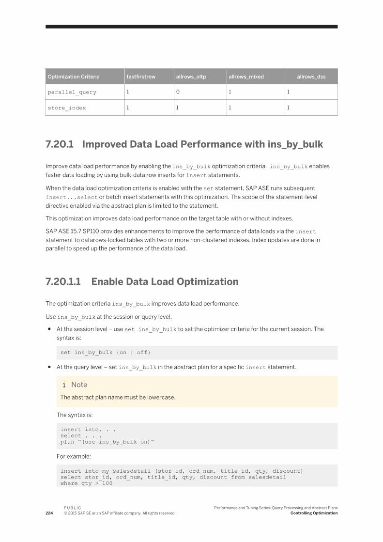
Optimization Criteria fastfirstrow allrows_oltp allrows_mixed allrows_dss
parallel_query 1 0 1 1
store_index 1 1 1 1
7.20.1 Improved Data Load Performance with ins_by_bulk
Improve data load performance by enabling the ins_by_bulk optimization criteria. ins_by_bulk enables faster data loading by using bulk-data row inserts for insert statements.
When the data load optimization criteria is enabled with the set statement, SAP ASE runs subsequent insert...select or batch insert statements with this optimization. The scope of the statement-level directive enabled via the abstract plan is limited to the statement.
This optimization improves data load performance on the target table with or without indexes.
SAP ASE 15.7 SP110 provides enhancements to improve the performance of data loads via the insert statement to datarows-locked tables with two or more non-clustered indexes. Index updates are done in parallel to speed up the performance of the data load.
7.20.1.1 Enable Data Load Optimization
The optimization criteria ins_by_bulk improves data load performance.
Use ins_by_bulk at the session or query level.
● At the session level – use set ins_by_bulk to set the optimizer criteria for the current session. The syntax is:
set ins_by_bulk {on | off}
● At the query level – set ins_by_bulk in the abstract plan for a specific insert statement.
NoteThe abstract plan name must be lowercase.
The syntax is:
insert into. . . select . . . plan “(use ins_by_bulk on)”
For example:
insert into my_salesdetail (stor_id, ord_num, title_id, qty, discount) select stor_id, ord_num, title_id, qty, discount from salesdetailwhere qty > 100
224P U B L I C© 2015 SAP SE or an SAP affiliate company. All rights reserved.
Performance and Tuning Series: Query Processing and Abstract PlansControlling Optimization

plan '(use ins_by_bulk on)'
You can use either syntax (session level or query level) within a stored procedure.
7.20.1.2 Tables with Indexes
Data load optimization with a target table that has indexes efficiently loads data pages while maintaining the index.
All rows are packed in a set of preallocated data pages and directly written to disk to improve data load performance. Recoverability is guaranteed.
When the target table defines indexes, the indexes are also maintained while writing data pages in bulk.
Noteins_by_bulk is supported for tables with and without indexes.
Slightly increased database space may be required when the existing pages are not full because insert...select when used with ins_by_bulk does not append rows to the existing pages, but allocates a new page when inserting the first rows.
7.20.1.3 Viewing Queries with bulkInsertRowCount
show_cached_plan_in_xml displays the cached execution plan with bulkInsertRowCount to indicate the bulk insert mode. The number enclosed in the bulkInsertRowCount tag is the row count inserted under bulk insert mode.
Context
This example shows that 10240 rows were inserted by bulk insert:
<Insert> <VA>1</VA> <est> <rowCnt>10240</rowCnt> <lio>9.749939</lio> <pio>9.749939</pio> <rowSz>2</rowSz> </est> <arity>1</arity> <bulkInsertRowCount>10240</bulkInsertRowCount> <TableScan> …… </TableScan> <objName>t1</objName> <dataIOSizeInKB>16</dataIOSizeInKB>
Performance and Tuning Series: Query Processing and Abstract PlansControlling Optimization
P U B L I C© 2015 SAP SE or an SAP affiliate company. All rights reserved. 225

<updateMode> Direct</updateMode> </Insert>
show_cached_plan_in_xml is not available for select into because select into statements are not cached in SAP ASE.
7.20.1.4 Batch Insert Optimization
Batch insert optimization is available when the insert statement is dynamically prepared and executed as a batch via Open Database Connectivity (ODBC).
Batch insert optimization avoids extra back and forth messages from the client to SAP ASE when insert...values statements uses dynamic parameters.
ins_by_bulk optimization further enhances batch insert performance by inserting rows in bulk mode internally.
The syntax is:
insert into <table> values (<param_1>, <param_2>, <param_3>)
Batch inserts also uses data-load optimization when ins_by_bulk is enabled.
For information about how to batch insert, see the ODBC Driver 15.7 Users Guide.
7.20.1.5 Data-Load Optimization on Tables with Multiple Indexes
Data-load optimization on a target table that has multiple indexes efficiently loads data pages and maintains multiple indexes in parallel.
To perform maintenance on multiple indexes in parallel, you must configure SAP ASE with resources (for example, threads), by setting:
● number of worker processes to the maximum that SAP ASE can use at any one time for all simultaneously running queries.
● max parallel degree to the maximum for a query. This parameter determines the maximum number of threads SAP ASE uses when processing a given query.
226P U B L I C© 2015 SAP SE or an SAP affiliate company. All rights reserved.
Performance and Tuning Series: Query Processing and Abstract PlansControlling Optimization

7.20.1.5.1 Viewing Parallel Update Index Queries in showplan
set showplan uses the update index operator to display parallel update index statements.
ExampleFor example:
set showplan on set ins_by_bulk ongo insert into my_authors select * from authors
This example showplan output is for an insert-select into a table with several indexes, executed with the data load optimizations. The text shown in bold reports the parallel index update enhancements.
QUERY PLAN FOR STATEMENT 1 (at line 2). Optimized using Parallel ModeExecuted in parallel by coordinating process and 2 worker processes. STEP 1 The type of query is INSERT. 5 operator(s) under root |ROOT:EMIT Operator (VA = 5) | | | INSERT Operator (VA = 4) | | The update mode is direct. | | | | |SCAN Operator (VA = 0) | | | FROM TABLE | | | authors | | | Table Scan. | | | Forward Scan. | | | Positioning at start of table. | | | Using I/O Size 16 Kbytes for data pages. | | | With LRU Buffer Replacement Strategy for data pages. | | | | |EXCHANGE Operator (VA = 3) (Merged) | | |Executed in parallel by 2 Producer and 1 Consumer processes.
| | | | | | |EXCHANGE:EMIT Operator (VA = 2) | | | | | | | | |UPDATE INDEX Operator (VA = 1) | | | | TO TABLE | | my_authors | | Using I/O Size 16 Kbytes for data pages. The INSERT OPERATOR (VA = 4) is using BULK INSERT (23 rows affected)
Without these data load enhancements, the data insertion is done in serial mode, with all the indexes being updated sequentially after the insertion of each row. With the enhanced data load optimizations, data pages are populated in bulk mode by one insert thread, followed by index updates which are performed by multiple threads each updating one or more indexes for all the data rows inserted on one page.
The line:
The INSERT OPERATOR (VA = 4) is using BULK INSERT
shows that bulk inserts are being performed.
Performance and Tuning Series: Query Processing and Abstract PlansControlling Optimization
P U B L I C© 2015 SAP SE or an SAP affiliate company. All rights reserved. 227

The plan fragment UPDATE INDEX Operator (VA = 1) shows that the index updates are being performed using parallel worker threads.
7.20.1.5.2 Viewing Queries with UpdateIndex
show_cached_plan_in_xml displays the cached execution plan using UpdateIndex to indicate that multiple indexes are applied in parallel.
Context
This example shows the UpdateIndex operator output that updates multiple indexes in parallel:
<EmitXchg> <Details> <VA>2</VA> <Vtuple Label="OutputVtuple"> <Collection Label="Columns(#1)"> <Column> (0x0x1497d6f00) type:INT1len:1 offset:0 valuebuf:0x(nil) status:(0x00000000)(constant:0x0x14a10e760 type:INT1 len:1 maxlen:1 ) </Column> </Collection> </Vtuple></Details> <UpdateIndex Label="UpdateIndex:"> <Details> <VA>1</VA> </Details> </UpdateIndex> </EmitXchg>
show_cached_plan_in_xml is not available for select into because select into statements are not cached in SAP ASE.
7.20.1.6 Restrictions
Data load optimization is not followed when certain scenarios are met.
Data-Load Optimization – Restrictions
Traditional row-by-row mode data load is used when:
● ins_by_bulk is not enabled in the plan clause or set statement.● The estimated page count to be inserted is fewer than eight pages (applies only to insert...select
statements).
228P U B L I C© 2015 SAP SE or an SAP affiliate company. All rights reserved.
Performance and Tuning Series: Query Processing and Abstract PlansControlling Optimization

● The target table is a system table.● The target table is a temporary table.● The target table is a remote table.● The target table is an all pages-locked (APL) table.● The target table contains foreign keys for referential integrity.● The target table is an in-memory database object.● Referential integrity or deferred referential integrity is defined on the target table.● full logging is not properly specified at the database, session, or query statement level.● The target table contains large object (LOB) columns.● The insert trigger is on the target table.● insert...values is used without parameters.● Source and target tables are the same.● The ignore_dup_key option is used with a unique index.● The batch insert query is not dynamically prepared.● The insert operator is issued from the alter table command.● Bulk insert is disabled while the following commands are underway concurrently when the data load is
attempted: .○ reorg rebuild ... with online○ create index ... with online
The insert instead performs in non-bulk mode, with serial index updates
Data-Load Optimization Using Parallel Index Updates – Restrictions
You cannot use data-load optimization:
● When no valid index is defined or only one index is in the target table.● The target table is a temporary table or a worktable.
The following behavior and restrictions are imposed when bulk insert is used in a transaction:
● Serial or concurrent data that is loaded using bulk inserts in a multistatement transaction is visible only to the inserting task while the transaction is active. While the transaction that loaded this data using bulk inserts remains active, concurrent access to this data by other tasks skips the uncommitted data.
● A single transaction can perform multiple bulk inserts to the same table multiple times. However, in a single transaction (whether it spans multiple databases, or only one), you can insert into a maximum number of four tables per database using this optimization.Bulk inserts are not applied to the fifth and subsequent tables in one transaction, and data load is performed in non-bulk mode, with serial index updates.
● Bulk insert is disabled while the following commands are underway concurrently when the data load is attempted. The insert instead performs in non-bulk mode, with serial index updates.○ reorg rebuild ... with online○ create index ... with online
● If the ddl in tran database option is enabled, an attempt to execute create index ...with online on a table following an insert bulk to that table in the same transaction is restricted. The create index operation is aborted, but the transaction remains active.
Performance and Tuning Series: Query Processing and Abstract PlansControlling Optimization
P U B L I C© 2015 SAP SE or an SAP affiliate company. All rights reserved. 229

Insert Bulk in a Transaction – Behavior and Restrictions
● Data loaded using bulk inserts in a multi-statement transaction is visible only to the inserting task while the transaction is active. While the transaction that loaded this data using bulk inserts is still active, concurrent access to this data by other tasks skips the uncommitted data.
● Concurrent data loads to the same table (or partition) from different tasks is supported. All data inserted during these concurrent data loads remains invisible to all tasks other than the inserting task until the inserting transaction commits.
● A single transaction can perform multiple bulk inserts to the same table multiple times. However, a maximum number of four tables per database can be inserted using this optimization in one transaction.For transactions that span multiple databases, each database has a maximum of four tables which is inserted using this optimization.Bulk inserts are not applied to the fifth and subsequent tables in one transaction, and data load is performed in non-bulk mode, with serial index updates.
● If the ddl in tran database option is enabled, an attempt to execute create index ...with online on a table following an insert bulk to that table in the same transaction is restricted. The create index operation is aborted, but the transaction remains active.
7.20.1.7 Downgrade Considerations
Transaction logs generated by the data-load optimizations and parallel index updates are incompatible with versions of SAP ASE earlier than 15.7 SP110. Database and transaction log dumps that are generated with data-load optimizations and parallel index updates cannot be recovered by earlier versions.
To downgrade an entire installation to an earlier version, use sp_downgrade, which truncates the active portion of the transaction log, thus permitting recovery of the databases by the earlier version.
See Reference Manual: Procedures.
To load a database containing transactional activity from the optimized data load, use sp_downgrade_esd to first downgrade it to the target support package version. This process clears transactional activity from the log, which then allows an earlier version to load and recover a dump of this database.
See the Installation Guide.
You cannot downgrade database dumps that contain log activity from the optimized data load and parallel index updates. Use the output from load...with headeronly to see if a particular dump contains such activity. To load such dumps into an earlier SAP ASE version that does not support these new optimizations (for example, SAP ASE 15.7 SP100), you must first reload the dump into an SAP ASE version that supports this feature. Then use sp_downgrade_esd to downgrade the database to the appropriate version. Re-create the dump from the downgraded database in a form that is compatible with the earlier SAP ASE version.
With some restrictions, database and transaction log dumps from a later version of SAP ASE can be loaded and recovered in earlier versions. However, once a dump is generated, it may be compatible with only a few of the earlier versions of SAP ASE, depending on the features used in the database, or the objects that are contained in the dumps.
Prior to generating the dumps, you can use the db_attr system function to identify the features that are currently active in the database, and the information that will be included in dumps.
230P U B L I C© 2015 SAP SE or an SAP affiliate company. All rights reserved.
Performance and Tuning Series: Query Processing and Abstract PlansControlling Optimization

7.20.1.8 Troubleshoot
Troubleshoot common situations that may cause bulk insert optimizations to not be applied.
● Check the showplan output to confirm that:○ The UPDATE INDEX operator is used.○ The INSERT OPERATOR is using BULK INSERT. It is possible at runtime SAP ASE decides to run the
query without BULK INSERT even though it was used during compile time.○ A sufficient number of worker threads is configured or available to perform the index updates in
parallel.
● If bulk insert does not execute, set trace flag 9586 to diagnose the reason in the XML output.
7.20.2 Enhancements to Insert Optimization with merge into
SAP ASE extends the bulk insert and parallel index updates for the insert portion of merge into statements. A new run-time optimization is also introduced for bulk insert.
Massive data loading and merging data from a transactional database into the data warehouse for increased analytics are common operations in the SAP® Business Information Warehouse (BW) environment. During the BW data-loading process query statement, merge into is frequently used to load data into an existing table or to update and delete existing rows.
Bulk-data performance is improved for the insert portion of merge into statements when a large volume of data is loaded with all rows logged, with and without an index. Noticeable performance improvement occurs when the source and target tables use a join predicate resulting in more insert operations, as opposed to update and delete operations. Improvements may not be significant for small source tables.
Additionally, SAP ASE now automatically decides to choose the bulk insert, and therefore parallel index updates, for insert select, batch insert and merge into based on the run-time statistics. In SAP ASE 15.7 SP100, this choice was hinted by the set command and optimizer hints.
7.20.2.1 Enabling Bulk Insert
The new sp_configure parameter enable bulk inserts defines the engine behavior at the system level for bulk inserts.
Context
Bulk insert is turned off when it is set to 0. When enable bulk inserts is set to 1, it attempts bulk insert by caching all inserted rows if all other conditions are satisfied. When more than the eight pre-defined threshold pages are inserted, it will go through bulk insert. Otherwise, normal non-bulk insert is used. The eight-page limit cannot be reconfigured.
Performance and Tuning Series: Query Processing and Abstract PlansControlling Optimization
P U B L I C© 2015 SAP SE or an SAP affiliate company. All rights reserved. 231

enable bulk inserts is added under the Query Tuning group and is not enabled by default.
Syntax:
sp_configure "enable bulk inserts"
Optimizer criteria ins_by_bulk can continue to be used to turn on or off bulk insert mode at the session or query level.
7.20.2.2 Automatic Selection of Bulk Insert
Bulk insert mode is automatically used when the new sp_configure parameter enable bulk inserts is set to 1, and bulk insert mode of more than eight data pages is detected in insert select, batch insert, or merge into statements.
If fewer than eight data pages is detected during insertion, non-bulk insert mode is used instead.
7.20.2.3 Determining When to Use in_by_bulk
Optimizer criteria ins_by_bulk should be used instead of enable bulk inserts to turn on bulk insert mode in certain scenarios.
Use ins_by_bulk to turn on or off bulk inserts when:
● You want to control bulk inserts at the session or query level.● You insert fewer than eight pages in bulk. Eight pages is the threshold limit for using enable bulk inserts.
Use showplan to verify the amount of rows inserted in bulk.● You have downgraded to SAP ASE 15.7 SP100.
You can set enable bulk inserts at the system level while still specifying ins_by_bulk at the session or query level. This table summarizes how they interact with each other:
enable bulk inserts = 0 (default)
enable bulk inserts = 1
set ins_by_bulk on Attempts bulk insert if the data rows inserted fills the threshold of eight pages. Reverts to non-bulk insert, if not enough rows are inserted.
Attempts bulk insert
set ins_by_bulk off Turns off bulk insert Turns off bulk insert
ins_by_bulk unspecified via set or plan clause (default)
Turns off bulk insert Attempts bulk insert
232P U B L I C© 2015 SAP SE or an SAP affiliate company. All rights reserved.
Performance and Tuning Series: Query Processing and Abstract PlansControlling Optimization

7.20.2.4 Transfer Data to a Target Table in Bulk
Insert operation performance is improved in merge into statements by applying bulk insert for single or multistatement transactions. Index maintenance performance is also improved by using parallel index updates.
In this example, bulk insert is applied as an insert operation of the merge statement when the search condition does not match. Indication of the bulk insert operation is not needed in the SQL statement since more than eight pages of data are filled.
merge into target_tab as Target using source_tab as Source ON Source.a1 = Target.a2 when matched then update set b2 = Source.b1 when not matched then insert(a2, b2, c2, d2) values(Source.a1, Source.b1, Source.c1, Source.d1)
Unique key is a1 of source_tab and a2 of target_tab respectively.
All the rows are packed in bulk to a set of new pages. As the generated data fills the page, the page is written to disk. When more than one index exists, the data page is also handed to the parallel index update module to maintain multiple indexes in parallel. In this bulk insert mode, every row insertion is fully logged.
7.20.2.5 Caching of Inserted Rows in merge into statement
When enable bulk inserts is on, rows are cached only before the decision to use bulk insert or not. After this decision, the rows are no longer cached.
Context
This run-time logic builds the rows directly into the memory cache. In the case of variable length of rows, when the remaining space in a page is not larger than the maximum length of the row, the row is built into a new page. After the row is built, it is moved to the remaining space of the last page (if space allows).
In most cases, the new run-time logic will not incur extra memory copy, however it does use more memory consumption, totaling a maximum of 8 pages x @@metathesized (as row cache) + page x @@maxpagesize (as row build buffer for the last rows), from procedure cache. In instances where there may not be enough memory for caching rows (for example, in a busy system), non-bulk insert is used.
Retrieve this information using the built-in function show_cached_plan_in_xml(). For cached statements, such as merge into, bulk insert information is displayed in the cached XML plan and the XML tag <bulkInsertRowCount> indicates the bulk insert mode.
In this example, the number 10 in bold is the row count inserted under bulk insert mode. The plan shows the bulk insert update for the merge into statement. The INSERT OPERATOR (VA = 3) has bulk inserted 10 rows. (Avg row size 527.500000).
select show_cached_plan_in_xml(1840622331,19,0) <Merge> <VA>3</VA>
Performance and Tuning Series: Query Processing and Abstract PlansControlling Optimization
P U B L I C© 2015 SAP SE or an SAP affiliate company. All rights reserved. 233

<est> <rowCnt>10</rowCnt> <lio>0</lio> <pio>0</pio> <rowSz>2</rowSz> </est> …… <dataIOSizeInKB>16</dataIOSizeInKB> <updateMode>Deferred</updateMode> <bulkInsertRowCount>10</bulkInsertRowCount> </Merge>
Changing enable bulk inserts will not invalidate a previous cached plan. To apply the change, you must first purge the query statement cache so that the query recompiles and a new plan executes. Similarly for the optimization criteria ins_by_bulk, the statement cache of the query should be purged to recompile and execute a new plan.
7.20.2.6 Viewing Bulk Inserted Rows in showplan
All inserted rows for merge into are logged. showplan displays the number of rows inserted under bulk mode.
For example:set showplan onset ins_by_bulk ongo
merge into t2 as Targetusing t1 as Source ON Source.a1 = Target.a2when matched then update set b2 = Source.b1when not matched then insert(a2, b2, c2) values(Source.a1, Source.b1, Source.c1)
| |MERGE Operator (VA = 6) | | The update mode is deferred.| || | |NESTED LOOP JOIN Operator (VA = 2) (Join Type: Left Outer Join)| | | | | | |SCAN Operator (VA = 0)| | | | FROM TABLE| | | | t1 ……| | |EXCHANGE Operator (VA = 5) (Merged)| | |Executed in parallel by 4 Producer and 1 Consumer processes.| | || | | |EXCHANGE:EMIT Operator (VA = 4)| | | || | | | |UPDATE INDEX Operator (VA = 3)| | | | TO TABLE| | T2| | Using I/O Size 16 Kbytes for data pagesThe MERGE OPERATOR (VA = 6) is using BULK INSERT(23 rows affected)
Even if the parallel index update operator is generated at compile time, it may choose serial index update at run time for some cases. showplan output provides information about whether it updates the indexes under
234P U B L I C© 2015 SAP SE or an SAP affiliate company. All rights reserved.
Performance and Tuning Series: Query Processing and Abstract PlansControlling Optimization

parallel or serial mode. For example, if parallel UPDATE INDEX Operator (VA = 3) has not been executed, the following message appears in the showplan output.
The parallel UPDATE INDEX Operator (VA = 3) has been disabled at run-time. Indexes updated in serial mode.
The LAVA plan tree does not change for the insert operator itself with merge into or other insert operations. However, the plan fragment about parallel index update is added, as shown in the previous example.
7.20.2.7 Restrictions
Data-load optimization is not followed when certain scenarios are met.
The bulk insert mode of an insert operator in insert select, batch insert, or merge into statements is not supported when:
● The estimated page count to be inserted is fewer than eight pages.● insert values(…) is used with constant values.● The ignore_dup_key option is used with a unique index.● The target table is an all-pages-locked (APL) table.● The target table is a remote table.● The target table is a system table.● The target table is a user’s temporary table.● The target table is an in-memory database object.● full logging is not properly specified at the database, session, or query statement level.● The batch insert query is not dynamically prepared.● The insert trigger is on the target table.● Referential integrity or foreign key is defined on the target table.● Large object (LOB) columns are defined on the target table.● The alter table command is used.● reorg build … with online is used.● create index … with online is used.
Performance and Tuning Series: Query Processing and Abstract PlansControlling Optimization
P U B L I C© 2015 SAP SE or an SAP affiliate company. All rights reserved. 235

7.21 Limiting Optimization Time
You can use the optimization timeout limit configuration parameter to restrict the amount of time spent optimizing a query.
Context
optimization timeout limit specifies the amount of time that is spent optimizing a query as a percentage of the total time spent processing the query.
The timeout is activated only if:
● At least one complete plan has been retained as the best plan, and● The optimization timeout limit has been exceeded.
Procedure
● Use sp_configure to set optimization timeout limit at the server level. For example, to limit optimization time to 10 percent of total query processing time, enter:
sp_configure “optimization timeout limit”, 10
● To set optimization timeout limit at the session level, use:
set plan optimeoutlimit <n>
This command overrides the server setting.
The default value is 10 percent; you can specify any value from 1 to 1000.
At the server level, there is a separate configuration parameter, optimization timeout limit, for the server-level default timeout value within stored procedure compilations. The default value is 40 percent; you can specify any value from 1 to 4000.
236P U B L I C© 2015 SAP SE or an SAP affiliate company. All rights reserved.
Performance and Tuning Series: Query Processing and Abstract PlansControlling Optimization

7.22 Controlling Parallel Optimization
The goal of executing queries in parallel is to get the fastest response time, even if it involves more total work from the server.
Procedure
Use these configuration parameters to enable and control parallel processing:
○ number of worker processes○ max parallel degree○ max resource granularity○ max repartition degree
With the exception of number of worker processes, each of these parameters can be set at the server and the session level. To view the current session-level value of a parameter, use the select command. For example, to view the current value of max resource granularity, enter:
select @@resource_granularity
NoteWhen set or viewed at the session level, these parameters do not include “max.”
7.22.1 number of worker processes Configuration Parameter
Use number of worker processes to specify the maximum number of worker processes to use at any one time for all simultaneously running parallel queries.
number of worker processes is a server-wide configuration parameter only; use sp_configure to set the parameter. For example, to set the maximum number of worker processes to 200, enter:
sp_configure “number of worker processes”, 200
Performance and Tuning Series: Query Processing and Abstract PlansControlling Optimization
P U B L I C© 2015 SAP SE or an SAP affiliate company. All rights reserved. 237

7.22.2 Specifying the Number of Worker Processes Available for Parallel Processing
Use max parallel degree, at either the session or server level, to specify the maximum number of worker processes allowed per query.
Procedure
● For example, to set max parallel degree to 60 at the server level, enter:
sp_configure “max parallel degree”, 60
● To set max parallel degree to 60 at the session level, enter:
set parallel_degree 60
The value of max parallel degree must be equal to or less than the current value of number of worker processes. Setting max parallel degree to 1 turns off parallel processing—SAP ASE scans all tables and indexes serially. To enable parallel partition scans, set max parallel degree equal to or greater than the number of partitions in the table you are querying.
7.22.3 Using max resource granularity to Specify Memory for a Single Query
Use max resource granularity, at either the session or server level, to specify the percentage of total memory allocated to a single query.
Procedure
● For example, to set max resource granularity to 35 percent at the server level, enter:
sp_configure “max resource granularity”, 35
● To set max resource granularity to 35 percent at the session level, enter:
set resource_granularity 35
The value of this parameter can affect the query optimizer’s choice of operators for a query. If the value max resource granularity is low, SAP ASE can choose many hash- and sort-based operators. max resource granularity also affects the scheduling algorithm in parallel optimization.
max resource granularity can affect dynamic buffer allocation in query execution and the amount of tempdb buffer cache used in update statistics.
238P U B L I C© 2015 SAP SE or an SAP affiliate company. All rights reserved.
Performance and Tuning Series: Query Processing and Abstract PlansControlling Optimization

7.22.4 Setting the Number of Worker Processes with max repartition degree
Use max repartition degree, at the session or server level, to suggest a number of worker processes that the query processor can use to partition a data stream.
Context
NoteThe value of max repartition degree is a suggestion only; the query processor decides the optimal number.
max repartition degree is most useful when the tables being queried are not partitioned, but partitioning the resultant data stream may improve performance by allowing concurrent SQL operations.
Procedure
● For example, to set max repartition degree to 15 at the server level, enter:
sp_configure “max repartition degree”, 15
● To set max repartition degree to 15 at the session level, enter:
set repartition_degree 15
The value of max repartition degree cannot exceed the current value of max parallel degree. SAP recommends that you set the value of this parameter equal to or less than the number of CPUs or disk systems that can work in parallel.
7.23 Concurrency Optimization for Small Tables
Table scans are not used for data-only-locked tables of 15 pages or fewer, if there is a useful index on the table. Instead, the optimizer selects the cheapest index that matches any search argument that can be optimized in the query.
The locking required for an index scan provides higher concurrency and reduces the chance of deadlocks, although slightly more I/O may be required than for a table scan.
If concurrency on small tables is not an issue, and you want to optimize the I/O instead, use sp_chgattribute to disable this optimization. For example, to turn off concurrency optimization for a table:
sp_chgattribute tiny_lookup_table,
Performance and Tuning Series: Query Processing and Abstract PlansControlling Optimization
P U B L I C© 2015 SAP SE or an SAP affiliate company. All rights reserved. 239

“concurrency_opt_threshold”, 0
With concurrency optimization disabled, the query processor can choose table scans when they require fewer I/Os.
You can also increase the concurrency optimization threshold for a table. This command sets the concurrency optimization threshold for a table to 30 pages:
sp_chgattribute lookup_table, “concurrency_opt_threshold”, 30
The maximum value for the concurrency optimization threshold is 32,767. Setting the value to -1 enforces concurrency optimization for a table of any size; this setting may be useful when a table scan is chosen over indexed access, and the resulting locking results in increased contention or deadlocks.
The current setting is stored in systabstats.conopt_thld and is printed as part of optdiag output.
7.23.1 Effects of Changing a Tables' Locking Scheme
Concurrency optimization affects only data-only-locked tables.
Table 10: Effects of alter table on Concurrency Optimization Settings
Changing From Effect on Stored Value
Allpages to data-only Set to 15, the default
Data-only to allpages Set to 0
One data-only scheme to another Configured value retained
7.24 Query Plan Optimization with Star Joins
A star join is a commonly used data warehouse query that runs against a star schema database, which consists of a large table (also known as a fact table) surrounded by dimension tables.
Fact tables typically include two types of columns: one that includes measurements, metrics, or facts about the business process, and another column that includes foreign keys to dimension tables. Dimension tables usually include descriptive attributes. For example, a fact table may include information about the number of hiking books sold by a particular author on a particular day. The corresponding dimension table includes the address, age, and gender of the author.
Star joins join the fact table with one or more dimension tables along the foreign keys. The star join may include filter predicates on the dimension tables (for example, where gender = 'M'), but it contains no joins between the dimension tables.
240P U B L I C© 2015 SAP SE or an SAP affiliate company. All rights reserved.
Performance and Tuning Series: Query Processing and Abstract PlansControlling Optimization

Snowflake schemas extend star joins by allowing each of the dimension tables to act as local fact tables and join with another set of dimension tables.
This star join joins the Orders fact table with the Time, Customer, and Location dimension tables:
select C.dattr, sum(O.measure1), count(*) from Orders O join Time T on O.key_dim1 = T.key_col join Customer C on O.key_dim2 = C.key_col join Location L on O.key_dim3 = L.key_colwhere T.dattr between 1 and 1000 and C.dattr between 1001 and 2000 and L.dattr between 901 and 1900group by C.dattr
To improve performance for star join query evaluation these changes have been made in version 16.0:
● For parallel plans, the bloom filter probe moves below the Xchg operator.● A new star join hint uses abstract plan to help the query processor better detect star join queries.● The final plan of any star join is now forced to use bloom filter under the use fact_table hint.● Hash joins and a join orders are forced based on the selectivities between fact and dimension tables for
the star join query under the use fact_table hint. The query processor adjusts the query plan to provide the greatest benefit from the bloom filter.
The query optimizer uses star joins when appropriate. You need not configure SAP ASE to use star joins. However, SAP does recommend that you enable the set join_bloom_filter option and parallel query processing when using star joins.
NoteWhen you set the optimization goal to allrows_dss, the query processor enables set join_bloom_filter and parallel query processing.
Performance and Tuning Series: Query Processing and Abstract PlansControlling Optimization
P U B L I C© 2015 SAP SE or an SAP affiliate company. All rights reserved. 241

7.24.1 Star Join HintThe use fact_table abstract plan hint specifies the central fact table in a star join query, and triggers special query plan optimization strategies for the query.
The syntax is:
PLAN '(use fact_table <fact_table_name_or_alias_name>)'
where:
● fact_table – indicates that the query includes a fact table from a star join.● <fact_table_name_or_alias_name> – specifies the name or alias name used for the central fact table.
In this example, F is the alias name:
use fact_table 'F'
For example, this joins the Orders fact table to the Time, Customer, and Location dimension tables:
select C.dattr, sum(O.measure1), count(*) from Orders Ojoin Time T on O.key_dim1 = T.key_coljoin Customer C on O.key_dim2 = C.key_coljoin Location L on O.key_dim3 = L.key_colwhere T.dattr between 1 and 1000and C.dattr between 1001 and 2000and L.dattr between 901 and 1900group by C.dattr plan '(use fact_table O)'
SAP ASE versions 16.0 SP01 PL01 and later allow you to include union-derived tables as dimension tables combined with a fact table hint. For example:
select ...from F join d1on F.c1 = d1.c1join d2on F.c2 = d2.c1join ( select ... from dt1 where ... union select ... from dt2 where ...)onjoin[...] plan '(use fact_table F)'
Versions of SAP ASE earlier than 16.0 SP01 PL01 successfully run this query but do not apply the fact table hint or the special optimization. That is, they ignore the fact table hint.
242P U B L I C© 2015 SAP SE or an SAP affiliate company. All rights reserved.
Performance and Tuning Series: Query Processing and Abstract PlansControlling Optimization

The use fact_table hint makes these changes to the query processor's star query detection algorithm and plan generation:
● The detection algorithm starts with the <fact_table_alias_name>. This table is always the center of a snowflake schema.
● Allows or clauses.● Allows joins between the fact table and the dimension tables to be multicolumn equijoins. You need not
include an explicit constraint definition between primary and foreign keys.● If the query processor cannot locate a good plan for the nested loop join while it generates the query plan
for the star join (typically due to missing indexes or less restrictive selectivities), it chooses a hash join plan with a forced join order. The join order is based on the selectivities between the dimension and the fact tables. The higher the selectivity (that is, a lower ratio value), the closer the dimension tables are in that join order to the fact table.
The query processor ignores the use fact_table hint unless the query meets these conditions:
● The query has at least three tables.● The query has no outer joins or nested subqueries.● The hinted fact table is the largest joining table within its query block.● The dimension tables and the fact table are joined with equijoins.● There are no join predicates between the dimension tables.
7.24.2 Star Join Query Plans Under the use fact_table Hint
The use fact_table abstract plan hint allows the query processor to chose a parallel hash join plan for the star join query. Parallel plans enable the query processor to push bloom filter probings (which allow for faster joins between dimension and fact tables) below the EXCHANGE operator, further reducing the number of qualifying rows from fact tables.
Versions of SAP ASE earlier than 16.0 included the bloom filter above the EXCHANGE operator in sp_showplan output.
This example includes a parallel plan under the hint, which includes table F as the hinted central fact table:
QUERY PLAN FOR STATEMENT 1 (at line 1). Optimized using Parallel ModeExecuted in parallel by coordinating process and 66 worker processes. STEP 1The type of query is SELECT.29 operator(s) under root|ROOT:EMIT Operator (VA = 29)|| |HASH VECTOR AGGREGATE Operator (VA = 28)| | GROUP BY| | Evaluate Grouped COUNT AGGREGATE.| | Evaluate Grouped SUM OR AVERAGE AGGREGATE.| | Evaluate Grouped SUM OR AVERAGE AGGREGATE.| | Evaluate Grouped SUM OR AVERAGE AGGREGATE.| | Evaluate Grouped SUM OR AVERAGE AGGREGATE.| | Evaluate Grouped SUM OR AVERAGE AGGREGATE.| | Evaluate Grouped SUM OR AVERAGE AGGREGATE.| | Evaluate Grouped SUM OR AVERAGE AGGREGATE.| | Evaluate Grouped SUM OR AVERAGE AGGREGATE.| | Evaluate Grouped SUM OR AVERAGE AGGREGATE.| | Evaluate Grouped SUM OR AVERAGE AGGREGATE.
Performance and Tuning Series: Query Processing and Abstract PlansControlling Optimization
P U B L I C© 2015 SAP SE or an SAP affiliate company. All rights reserved. 243

| | Evaluate Grouped SUM OR AVERAGE AGGREGATE.| | Evaluate Grouped SUM OR AVERAGE AGGREGATE.| | Evaluate Grouped SUM OR AVERAGE AGGREGATE.| | Evaluate Grouped SUM OR AVERAGE AGGREGATE.| | Evaluate Grouped SUM OR AVERAGE AGGREGATE.| | Evaluate Grouped SUM OR AVERAGE AGGREGATE.| | Using Worktable10 for internal storage.| | Key Count: 3| || | |HASH JOIN PROBE Operator (VA = 27) (Join Type: Inner Join)| | | Using Worktable1 for internal storage.| | | Key Count: 1| | || | | |HASH JOIN BUILD Operator (VA = 1) (Join Type: Inner Join)| | | | Using Worktable1 for internal storage.| | | | Key Count: 1| | | || | | | |SCAN Operator (VA = 0)| | | | | FROM TABLE| | | | | /B49/DBENCH01P| | | | | DP| | | | | Index : /B49/DBENCH01P~010| | | | | Forward Scan.| | | | | Positioning by key.| | | | | Keys are:| | | | | SID_0CHNGID ASC| | | | | SID_0RECORDTP ASC| | | | | SID_0REQUID ASC| | | | | Using I/O Size 16 Kbytes for index leaf pages.| | | | | With LRU Buffer Replacement Strategy for index leaf pages.| | | | | Using I/O Size 16 Kbytes for data pages.| | | | | With LRU Buffer Replacement Strategy for data pages.| | || | | |HASH JOIN PROBE Operator (VA = 26) (Join Type: Inner Join)| | | | Using Worktable2 for internal storage.| | | | Key Count: 1| | | || | | | |HASH JOIN BUILD Operator (VA = 3) (Join Type: Inner Join)| | | | | Using Worktable2 for internal storage.| | | | | Key Count: 1| | | | || | | | | |SCAN Operator (VA = 2)| | | | | | FROM TABLE| | | | | | /B49/DBENCH01U| | | | | | DU| | | | | | Index : "/B49/DBENCH01U~020"| | | | | | Forward Scan.| | | | | | Positioning at index start.| | | | | | Using I/O Size 16 Kbytes for index leaf pages.| | | | | | With LRU Buffer Replacement Strategy for index leaf pages.| | | | | | Using I/O Size 16 Kbytes for data pages.| | | | | | With LRU Buffer Replacement Strategy for data pages.| | | || | | | |HASH JOIN PROBE Operator (VA = 25) (Join Type: Inner Join)| | | | | Using Worktable3 for internal storage.| | | | | Key Count: 2| | | | || | | | | |HASH JOIN BUILD Operator (VA = 5) (Join Type: Inner Join)| | | | | | Using Worktable3 for internal storage.| | | | | | Key Count: 2| | | | | || | | | | | |SCAN Operator (VA = 4)| | | | | | | FROM TABLE| | | | | | | /B49/DBENCH01T| | | | | | | DT| | | | | | | Index : /B49/DBENCH01T~20| | | | | | | Forward Scan.| | | | | | | Positioning by key.
244P U B L I C© 2015 SAP SE or an SAP affiliate company. All rights reserved.
Performance and Tuning Series: Query Processing and Abstract PlansControlling Optimization

| | | | | | | Keys are:| | | | | | | SID_0CALMONTH ASC| | | | | | | Using I/O Size 16 Kbytes for index leaf pages.| | | | | | | With LRU Buffer Replacement Strategy for index leaf pages.| | | | | | | Using I/O Size 16 Kbytes for data pages.| | | | | | | With LRU Buffer Replacement Strategy for data pages.| | | | || | | | | |HASH JOIN PROBE Operator (VA = 24) (Join Type: Inner Join)| | | | | | Using Worktable4 for internal storage.| | | | | | Key Count: 1| | | | | || | | | | | |HASH JOIN BUILD Operator (VA = 7) (Join Type: Inner Join)| | | | | | | Using Worktable4 for internal storage.| | | | | | | Building pushdown bloom filter (bv7)| | | | | | | Key Count: 1| | | | | | || | | | | | | |SCAN Operator (VA = 6)| | | | | | | | FROM TABLE| | | | | | | | /B49/XCUSTOMER| | | | | | | | X1| | | | | | | | Table Scan.| | | | | | | | Forward Scan.| | | | | | | | Positioning at start of table.| | | | | | | | Using I/O Size 128 Kbytes for data pages.| | | | | | | | With LRU Buffer Replacement Strategy for data pages.| | | | | || | | | | | |HASH JOIN PROBE Operator (VA = 23) (Join Type: Inner Join)| | | | | | | Using Worktable5 for internal storage.| | | | | | | Key Count: 1| | | | | | || | | | | | | |HASH JOIN BUILD Operator (VA = 9) (Join Type: Inner Join)| | | | | | | | Using Worktable5 for internal storage.| | | | | | | | Building pushdown bloom filter (bv9)| | | | | | | | Key Count: 1| | | | | | | || | | | | | | | |SCAN Operator (VA = 8)| | | | | | | | | FROM TABLE| | | | | | | | | /B49/DBENCH011| | | | | | | | | D1| | | | | | | | | Table Scan.| | | | | | | | | Forward Scan.| | | | | | | | | Positioning at start of table.| | | | | | | | | Using pushdown bloom filter (bv7).| | | | | | | | | Using I/O Size 128 Kbytes for data pages.| | | | | | | | | With LRU Buffer Replacement Strategy for data pages.| | | | | | || | | | | | | |EXCHANGE Operator (VA = 22) (Merged)| | | | | | | |Executed in parallel by 64 Producer and 1 Consumer processes.| | | | | | | || | | | | | | | |EXCHANGE:EMIT Operator (VA = 21)| | | | | | | | || | | | | | | | | |HASH JOIN PROBE Operator (VA = 20) (Join Type: Inner Join)| | | | | | | | | | Using Worktable9 for internal storage.| | | | | | | | | | Key Count: 1| | | | | | | | | || | | | | | | | | | |EXCHANGE Operator (VA = 13) (Replicated)| | | | | | | | | | |Executed in parallel by 1 Producer and 64 Consumer processes.| | | | | | | | | | || | | | | | | | | | | |EXCHANGE:EMIT Operator (VA = 12)| | | | | | | | | | | || | | | | | | | | | | | |HASH JOIN BUILD Operator (VA = 11) (Join Type: Inner Join)| | | | | | | | | | | | | Using Worktable6 for internal storage.| | | | | | | | | | | | | Building pushdown bloom filter (bv11)| | | | | | | | | | | | | Key Count: 1| | | | | | | | | | | | || | | | | | | | | | | | | |SCAN Operator (VA = 10)
Performance and Tuning Series: Query Processing and Abstract PlansControlling Optimization
P U B L I C© 2015 SAP SE or an SAP affiliate company. All rights reserved. 245

| | | | | | | | | | | | | | FROM TABLE| | | | | | | | | | | | | | /B49/SSALESORG| | | | | | | | | | | | | | S1| | | | | | | | | | | | | | Index : "/B49/SSALESORG~0"| | | | | | | | | | | | | | Forward Scan.| | | | | | | | | | | | | | Positioning by key.| | | | | | | | | | | | | | Keys are:| | | | | | | | | | | | | | /B49/S_SALESORG ASC| | | | | | | | | | | | | | Using I/O Size 16 Kbytes for index leaf pages.| | | | | | | | | | | | | | With LRU Buffer Replacement Strategy for index leaf pages.| | | | | | | | | | | | | | Using I/O Size 16 Kbytes for data pages.| | | | | | | | | | | | | | With LRU Buffer Replacement Strategy for data pages.| | | | | | | | | || | | | | | | | | | |HASH JOIN PROBE Operator (VA = 19) (Join Type: Inner Join)| | | | | | | | | | | Using Worktable8 for internal storage.| | | | | | | | | | | Key Count: 1| | | | | | | | | | || | | | | | | | | | | |EXCHANGE Operator (VA = 17) (Replicated)| | | | | | | | | | | |Executed in parallel by 1 Producer and 64 Consumer processes.| | | | | | | | | | | || | | | | | | | | | | | |EXCHANGE:EMIT Operator (VA = 16)| | | | | | | | | | | | || | | | | | | | | | | | | |HASH JOIN BUILD Operator (VA = 15) (Join Type: Inner Join)| | | | | | | | | | | | | | Using Worktable7 for internal storage.| | | | | | | | | | | | | | Building pushdown bloom filter (bv15)| | | | | | | | | | | | | | Key Count: 1| | | | | | | | | | | | | || | | | | | | | | | | | | | |SCAN Operator (VA = 14)| | | | | | | | | | | | | | | FROM TABLE| | | | | | | | | | | | | | | /B49/DBENCH013| | | | | | | | | | | | | | | D3| | | | | | | | | | | | | | | Table Scan.| | | | | | | | | | | | | | | Forward Scan.| | | | | | | | | | | | | | | Positioning at start of table.| | | | | | | | | | | | | | | Using pushdown bloom filter (bv11).| | | | | | | | | | | | | | | Using I/O Size 128 Kbytes for data pages.| | | | | | | | | | | | | | | With LRU Buffer Replacement Strategy for data pages.| | | | | | | | | | || | | | | | | | | | | |SCAN Operator (VA = 18)| | | | | | | | | | | | FROM TABLE| | | | | | | | | | | | /B49/FBENCH01| | | | | | | | | | | | F| | | | | | | | | | | | Index : /B49/FBENCH01~060| | | | | | | | | | | | Forward Scan.| | | | | | | | | | | | Positioning at index start.| | | | | | | | | | | | Using pushdown bloom filter (bv15, bv9).| | | | | | | | | | | | Executed in parallel with a 64-way partition scan.| | | | | | | | | | | | Using I/O Size 128 Kbytes for index leaf pages.| | | | | | | | | | | | With LRU Buffer Replacement Strategy for index leaf pages.| | | | | | | | | | | | Using I/O Size 128 Kbytes for data pages.| | | | | | | | | | | | With MRU Buffer Replacement Strategy for data pages.
This example includes a serial plan under the hint:
QUERY PLAN FOR STATEMENT 1 (at line 1). Optimized using Serial ModeSTEP 1The type of query is SELECT.8 operator(s) under root|ROOT:EMIT Operator (VA = 8)|| |HASH VECTOR AGGREGATE Operator (VA = 7)
246P U B L I C© 2015 SAP SE or an SAP affiliate company. All rights reserved.
Performance and Tuning Series: Query Processing and Abstract PlansControlling Optimization

| | GROUP BY| | Evaluate Grouped COUNT AGGREGATE.| | Evaluate Grouped SUM OR AVERAGE AGGREGATE.| | Using Worktable4 for internal storage.| | Key Count: 1| || | |HASH JOIN Operator (VA = 6) (Join Type: Inner Join)| | | Using Worktable3 for internal storage.| | | Building pushdown bloom filter (bv6)| | | Key Count: 1| | || | | |SCAN Operator (VA = 0)| | | | FROM TABLE| | | | Location| | | | L| | | | Table Scan.| | | | Forward Scan.| | | | Positioning at start of table.| | | | Using I/O Size 2 Kbytes for data pages.| | | | With LRU Buffer Replacement Strategy for data pages.| | || | | |HASH JOIN Operator (VA = 5) (Join Type: Inner Join)| | | | Using Worktable2 for internal storage.| | | | Building pushdown bloom filter (bv5)| | | | Key Count: 1| | | || | | | |SCAN Operator (VA = 1)| | | | | FROM TABLE| | | | | Customer| | | | | C| | | | | Table Scan.| | | | | Forward Scan.| | | | | Positioning at start of table.| | | | | Using I/O Size 2 Kbytes for data pages.| | | | | With LRU Buffer Replacement Strategy for data pages.| | | || | | | |HASH JOIN Operator (VA = 4) (Join Type: Inner Join)| | | | | Using Worktable1 for internal storage.| | | | | Building pushdown bloom filter (bv4)| | | | | Key Count: 1| | | | || | | | | |SCAN Operator (VA = 2)| | | | | | FROM TABLE| | | | | | Time| | | | | | T| | | | | | Table Scan.| | | | | | Forward Scan.| | | | | | Positioning at start of table.| | | | | | Using I/O Size 2 Kbytes for data pages.| | | | | | With LRU Buffer Replacement Strategy for data pages.| | | | || | | | | |SCAN Operator (VA = 3)| | | | | | FROM TABLE| | | | | | Orders| | | | | | O| | | | | | Table Scan.| | | | | | Forward Scan.| | | | | | Positioning at start of table.| | | | | | Using pushdown bloom filter (bv4, bv5, bv6).| | | | | | Using I/O Size 2 Kbytes for data pages.| | | | | | With LRU Buffer Replacement Strategy for data pages.
Performance and Tuning Series: Query Processing and Abstract PlansControlling Optimization
P U B L I C© 2015 SAP SE or an SAP affiliate company. All rights reserved. 247

8 Optimization for Cursors
Cursors let you access the results of a SQL select statement one row at a time (or several rows, if you use set cursors rows).
You can think of a cursor as a “handle” on the result set of a select statement.
This figure shows a cursor accessing the authors table:
Since cursors use a different model from ordinary set-oriented SQL, the way cursors use memory and hold locks has performance implications for your applications. In particular, cursor performance issues include locking at the page and at the table level, network resources, and overhead of processing instructions.
8.1 Set-Oriented Versus Row-Oriented Programming
SQL was conceived as a set-oriented language. SAP ASE is extremely efficient when it works in set-oriented mode.
Cursors are required by ANSI SQL standards; when they are needed, they are very powerful. However, they can have a negative effect on performance.
For example, this query performs the identical action on all rows that match the condition in the where clause:
update titles set contract = 1 where type = ’business’
The optimizer finds the most efficient way to perform the update. In contrast, a cursor would examine each row and perform single-row updates if the conditions were met. The application declares a cursor for a select statement, opens the cursor, fetches a row, processes it, goes to the next row, and so forth. The application may perform quite different operations depending on the values in the current row, and the server’s overall use of resources for the cursor application may be less efficient than the server’s set level operations. However, cursors can provide more flexibility than set-oriented programming.
This figure illustrates the steps involved in using cursors. The function of cursors is to get to the middle box, where the user or application code examines a row and decides what to do, based on its values.
248P U B L I C© 2015 SAP SE or an SAP affiliate company. All rights reserved.
Performance and Tuning Series: Query Processing and Abstract PlansOptimization for Cursors

Figure 2: Cursor Flowchart
Here is a simple example of a cursor with the “Process Rows” step shown above in pseudocode:
declare biz_book cursor for select * from titles where type = ’business’goopen biz_bookgofetch biz_bookgo/* Look at each row in turn and perform** various tasks based on values, ** and repeat fetches, until** there are no more rows*/close biz_bookgodeallocate cursor biz_book go
Depending on the content of the row, the user might delete the current row:
delete titles where current of biz_book
or update the current row:
update titles set title="The Rich Executive’s Database Guide" where current of biz_book
Performance and Tuning Series: Query Processing and Abstract PlansOptimization for Cursors
P U B L I C© 2015 SAP SE or an SAP affiliate company. All rights reserved. 249
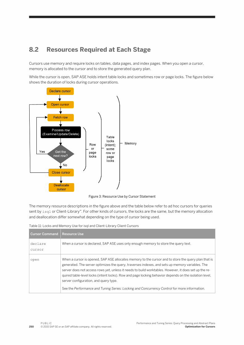
8.2 Resources Required at Each Stage
Cursors use memory and require locks on tables, data pages, and index pages. When you open a cursor, memory is allocated to the cursor and to store the generated query plan.
While the cursor is open, SAP ASE holds intent table locks and sometimes row or page locks. The figure below shows the duration of locks during cursor operations.
Figure 3: Resource Use by Cursor Statement
The memory resource descriptions in the figure above and the table below refer to ad hoc cursors for queries sent by isql or Client-Library™. For other kinds of cursors, the locks are the same, but the memory allocation and deallocation differ somewhat depending on the type of cursor being used.
Table 11: Locks and Memory Use for isql and Client-Library Client Cursors
Cursor Command Resource Use
declare cursor
When a cursor is declared, SAP ASE uses only enough memory to store the query text.
open When a cursor is opened, SAP ASE allocates memory to the cursor and to store the query plan that is generated. The server optimizes the query, traverses indexes, and sets up memory variables. The server does not access rows yet, unless it needs to build worktables. However, it does set up the required table-level locks (intent locks). Row and page locking behavior depends on the isolation level, server configuration, and query type.
See the Performance and Tuning Series: Locking and Concurrency Control for more information.
250P U B L I C© 2015 SAP SE or an SAP affiliate company. All rights reserved.
Performance and Tuning Series: Query Processing and Abstract PlansOptimization for Cursors

Cursor Command Resource Use
fetch When a fetch is executed, SAP ASE gets the row(s) required and reads specified values into the cursor variables or sends the row to the client. If the cursor needs to hold lock on rows or pages, the locks are held until a fetch moves the cursor off the row or page or until the cursor is closed. The lock is either a shared or an update lock, depending on how the cursor is written.
close When a cursor is closed, SAP ASE releases the locks and some of the memory allocation. You can open the cursor again, if necessary.
deallocate cursor
When a cursor is deallocated, SAP ASE releases the rest of the memory resources used by the cursor. To reuse the cursor, declare it again.
The descriptions for declare cursor and deallocate cursor in above refer to ad hoc cursors that are sent by isql or Client-Library. Other kinds of cursors allocate memory differently:
● For cursors that are declared on stored procedures, only a small amount of memory is allocated at declare cursor time. Cursors declared on stored procedures are sent using Client-Library or the precompiler and are known as execute cursors.
● For cursors declared within a stored procedure, memory is already available for the stored procedure, and the declare statement does not require additional memory.
8.3 Cursor Modes
There are two cursor modes: read-only and update. Read-only cursors can only display data from a select statement; update cursors can perform positioned updates and deletes.
Read-only mode uses shared page or row locks. If read committed with lock is set to 0, and the query runs at isolation level 1, it uses instant duration locks, and does not hold the page or row locks until the next fetch.
Read-only mode is in effect when you specify for read only or when the cursor’s select statement uses distinct, group by, union, or aggregate functions, and in some cases, an order by clause.
Update mode uses update page or row locks. It is in effect when:
● You specify for update.● The select statement does not include distinct, group by, union, a subquery, aggregate functions,
or the at isolation read uncommitted clause.● You specify shared.
If <column_name_list> is specified, only those columns are updatable.
See the Performance and Tuning Series: Locking and Concurrency Control for more information.
Specify the cursor mode when you declare the cursor. If the select statement includes certain options, the cursor is not updatable even if you declare it for update.
Performance and Tuning Series: Query Processing and Abstract PlansOptimization for Cursors
P U B L I C© 2015 SAP SE or an SAP affiliate company. All rights reserved. 251

8.4 Index Use and Requirements for Cursors
When a query is used in a cursor, it may require or choose different indexes than the same query used outside of a cursor.
Allpages-Locked Tables
For read-only cursors, queries at isolation level 0 (dirty reads) require a unique index. Read-only cursors at isolation level 1 or 3 should produce the same query plan as the select statement outside of a cursor.
The index requirements for updatable cursors mean that updatable cursors may use different query plans than read-only cursors. Updatable cursors have these indexing requirements:
● If the cursor is not declared for update, a unique index is preferred over a table scan or a nonunique index.● If the cursor is declared for update without a for update of list, a unique index is required on allpages-
locked tables. An error is raised if no unique index exists.● If the cursor is declared for update with a for update of list, then only a unique index without any
columns from the list can be chosen on an allpages-locked table. An error is raised if no unique index qualifies.
When cursors are involved, an index that contains an IDENTITY column is considered unique, even if the index is not declared unique. In some cases, IDENTITY columns must be added to indexes to make them unique, or the optimizer might be forced to choose a suboptimal query plan for a cursor query.
Data-Only-Locked Tables
In data-only-locked tables, fixed row IDs are used to position cursor scans, so unique indexes are not required for dirty reads or updatable cursors. The only cause for different query plans in updatable cursors is that table scans are used if columns from only useful indexes are included in the for update of list.
You can use table scans to avoid the Halloween problem, which is an update anomaly that can occur when a client using a cursor updates a column of the cursor result-set row, and that column defines the order in which the rows are returned from the table.
For example, if a cursor was to use an index on last_name and first_name and update one of these columns, the row could appear in the result set a second time.
To avoid the Halloween problem on data-only-locked tables, SAP ASE chooses a table scan when the columns from an otherwise useful index are included in the column list of a for update clause.
For implicitly updatable cursors declared without a for update clause, and for cursors where the column list in the for update clause is empty, cursors that update a column in the index used by the cursor may encounter the Halloween problem.
252P U B L I C© 2015 SAP SE or an SAP affiliate company. All rights reserved.
Performance and Tuning Series: Query Processing and Abstract PlansOptimization for Cursors

8.5 Comparing Performance with and Without Cursors
You can evaluate the performance of stored procedures written with and without cursors.
● With a cursor – the procedure makes only one pass through the table.● Without a cursor – the procedure scans the table and makes changes. For example, based on the sample
below, the table is scanned three times and the price of each book is changed.
In both examples, there is a unique index on titles(title_id).
In the example below, which shows statistics gathered against a 5000-row table, the cursor code takes over 4 times longer, even though it scans the table only once.
Table 12: Sample execution times against a 5000-row table
Procedure Access Method Time
increase_price Uses three table scans 28 seconds
increase_price_cursor Uses cursor, single table scan 125 seconds
Results from tests like these can vary widely. They are most pronounced on systems that have busy networks, a large number of active database users, and multiple users accessing the same table.
In addition to locking, cursors involve more network activity than set operations and incur the overhead of processing instructions. The application program needs to communicate with SAP ASE regarding every result row of the query. This is why the cursor code took much longer to complete than the code that scanned the table three times.
Cursor performance issues include:
● Locking at the page and table level● Network resources● Overhead of processing instructions
If there is a set-level programming equivalent, it may be preferable, even if it involves multiple table scans.
Sample Stored Procedure Written Without a Cursor
This is an example of a stored procedure without cursors.
/* Increase the prices of books in the ** titles table as follows:** ** If current price is <= $30, increase it by 20%** If current price is > $30 and <= $60, increase ** it by 10%** If current price is > $60, increase it by 5%**** All price changes must take effect, so this is** done in a single transaction.*/create procedure increase_priceas
Performance and Tuning Series: Query Processing and Abstract PlansOptimization for Cursors
P U B L I C© 2015 SAP SE or an SAP affiliate company. All rights reserved. 253

/* start the transaction */ begin transaction /* first update prices > $60 */ update titles set price = price * 1.05 where price > $60 /* next, prices between $30 and $60 */ update titles set price = price * 1.10 where price > $30 and price <= $60 /* and finally prices <= $30 */ update titles set price = price * 1.20 where price <= $30 /* commit the transaction */ commit transaction return
Sample Stored Procedure Written Without a Cursor
This procedure performs the same changes to the underlying table as the procedure written without a cursor, but it uses cursors instead of set-oriented programming. As each row is fetched, examined, and updated, a lock is held on the appropriate data page. Also, as the comments indicate, each update commits as it is made, since there is no explicit transaction.
/* Same as previous example, this time using a ** cursor. Each update commits as it is made.*/create procedure increase_price_cursorasdeclare @price money/* declare a cursor for the select from titles */declare curs cursor for select price from titles for update of price/* open the cursor */open curs/* fetch the first row */fetch curs into @price/* now loop, processing all the rows** @@sqlstatus = 0 means successful fetch** @@sqlstatus = 1 means error on previous fetch** @@sqlstatus = 2 means end of result set reached*/while (@@sqlstatus != 2)begin /* check for errors */ if (@@sqlstatus = 1) begin print "Error in increase_price" return end /* next adjust the price according to the ** criteria */ if @price > $60 select @price = @price * 1.05 else if @price > $30 and @price <= $60 select @price = @price * 1.10
254P U B L I C© 2015 SAP SE or an SAP affiliate company. All rights reserved.
Performance and Tuning Series: Query Processing and Abstract PlansOptimization for Cursors

else if @price <= $30 select @price = @price * 1.20 /* now, update the row */ update titles set price = @price where current of curs /* fetch the next row */ fetch curs into @priceend/* close the cursor and return */close curs return
8.6 Locking with Read-Only Cursors
You can write cursor code that enables you to display the locks that are set up at each point in the life of a cursor.
This example uses an allpages-locked table. Execute the code below, and pause at the arrows to execute sp_lock and examine the locks that are in place.
Figure 4: Read-Only Cursors and Locking Experiment Input
The results are listed below.
Table 13: Locks Held on Data and Index Pages by Cursors
Event Data Page
After declare No cursor-related locks.
After open Shared intent lock on authors.
After first fetch Shared intent lock on authors and shared page lock on a page in authors.
After 100 fetches Shared intent lock on authors and shared page lock on a different page in authors.
Performance and Tuning Series: Query Processing and Abstract PlansOptimization for Cursors
P U B L I C© 2015 SAP SE or an SAP affiliate company. All rights reserved. 255

Event Data Page
After close No cursor-related locks.
If you issue another fetch command after the last row of the result set has been fetched, the locks on the last page are released, so there will be no cursor-related locks.
With a data-only-locked table:
● If the cursor query runs at isolation level 1, and read committed with lock is set to 0, you do not see any page or row locks. The values are copied from the page or row, and the lock is immediately released.
● If read committed with lock is set to 1 or if the query runs at isolation level 2 or 3, you see either shared page or shared row locks at the point that the table above indicates shared page locks. If the table uses datarows locking, the sp_lock report includes the row ID of the fetched row.
8.7 Isolation Levels And Cursors
The query plan for a cursor is compiled and optimized when the cursor is opened. You cannot open a cursor and then use set transaction isolation level to change the isolation level at which the cursor operates.
Since cursors using isolation level 0 are compiled differently from those using other isolation levels, you cannot open a cursor at isolation level 0 and open or fetch from it at level 1 or 3. Similarly, you cannot open a cursor at level 1 or 3 and then fetch from it at level 0. Attempts to fetch from a cursor at an incompatible level result in an error message.
Once the cursor has been opened at a particular isolation level, you must deallocate the cursor before changing isolation levels. The effects of changing isolation levels while the cursor is open are as follows:
● Attempting to close and reopen the cursor at another isolation level fails with an error message.● Attempting to change isolation levels without closing and reopening the cursor has no effect on the
isolation level in use and does not produce an error message.
You can include an at isolation clause in the cursor to specify an isolation level. The cursor in the example below can be declared at level 1 and fetched from level 0 because the query plan is compatible with the isolation level:
declare cprice cursor for select title_id, price from titles where type = "business" at isolation read uncommitted
256P U B L I C© 2015 SAP SE or an SAP affiliate company. All rights reserved.
Performance and Tuning Series: Query Processing and Abstract PlansOptimization for Cursors

8.8 Partitioned Heap Tables and Cursors
A cursor scan of an unpartitioned heap table can read all data up to and including the final insertion made to that table, even if insertions took place after the cursor scan started.
If a heap table is partitioned, data can be inserted into one of the many page chains. The physical insertion point may be before or after the current position of a cursor scan. This means that a cursor scan against a partitioned table is not guaranteed to scan the final insertions made to that table.
NoteIf cursor operations require all inserts to be made at the end of a single page chain, do not partition the table used in the cursor scan.
8.9 Optimizing Tips for Cursors
There are a number of ways you can optimize cursors.
Optimizing for Cursor Selects Using a Cursor
A standalone select statement may be optimized very differently than the same select statement in an implicitly or explicitly updatable cursor.
When you are developing applications that use cursors, always check your query plans and I/O statistics using the cursor, rather than using a standalone select. In particular, index restrictions of updatable cursors require very different access methods.
Using union Instead of or Clauses or in Lists
Cursors cannot use the dynamic index of row IDs generated by the OR strategy.
Queries that use the OR strategy in standalone select statements usually perform table scans using read-only cursors. Updatable cursors may need to use a unique index and still require access to each data row, in sequence, in order to evaluate the query clauses.
A read-only cursor using union creates a worktable when the cursor is declared, and sorts it to remove duplicates. Fetches are performed on the worktable. A cursor using union all can return duplicates and does not require a worktable.
Performance and Tuning Series: Query Processing and Abstract PlansOptimization for Cursors
P U B L I C© 2015 SAP SE or an SAP affiliate company. All rights reserved. 257

Declaring the Cursor’s Intent
Always declare a cursor’s intent: read-only or updatable. This gives you greater control over concurrency implications.
If you do not specify the intent, SAP ASE decides for you, and very often it chooses updatable cursors. Updatable cursors use update locks, thereby preventing other update locks or exclusive locks. If the update changes an indexed column, the optimizer may need to choose a table scan for the query, resulting in potentially difficult concurrency problems. Be sure to examine the query plans for queries that use updatable cursors.
Specifying Column Names in the for update Clause
SAP ASE acquires update locks on the pages or rows of all tables that have columns listed in the for update clause of the cursor select statement. If the for update clause is not included in the cursor declaration, all tables referenced in the from clause acquire update locks.
The following query includes the name of the column in the for update clause, but acquires update locks only on the titles table, since price is mentioned in the for update clause. The table uses allpages locking. The locks on authors and titleauthor are shared page locks:
declare curs3 cursor forselect au_lname, au_fname, price from titles t, authors a, titleauthor tawhere advance <= $1000 and t.title_id = ta.title_id and a.au_id = ta.au_id for update of price
The table below shows the effects of:
● Omitting the for update clause entirely—no shared clause● Omitting the column name from the for update clause● Including the name of the column to be updated in the for update clause● Adding shared after the name of the titles table while using for update of price
In this table, the additional locks, or more restrictive locks for the two versions of the for update clause are emphasized.
Table 14: Effects of for update Clause and shared on cursor Locking
Clause titles authors titleauthor
Nonesh_page on data
sh_page on index
sh_page on datash_page on data
for update updpage on index
updpage on data
updpage on index
updpage on dataupdpage on data
258P U B L I C© 2015 SAP SE or an SAP affiliate company. All rights reserved.
Performance and Tuning Series: Query Processing and Abstract PlansOptimization for Cursors

Clause titles authors titleauthor
for update of priceupdpage on data
sh_page on index
sh_page on datash_page on data
for update of price + shared
sh_page on datash_page on index
sh_page on datash_page on data
Using set cursor Rows
The SQL standard specifies a one-row fetch for cursors, which wastes network bandwidth.
Using the set cursor rows query option and Open Client’s transparent buffering of fetches, you can improve performance:
ct_cursor(CT_CURSOR_ROWS)
Be careful when you choose the number of rows returned for frequently executed applications using cursors—tune them to the network.
See the Performance and Tuning Series: Basics for an explanation of this process.
Keeping Cursors Open Across Commits and Rollbacks
ANSI closes cursors at the conclusion of each transaction.
Transact-SQL provides the set option close on endtran for applications that must meet ANSI behavior. By default, however, this option is turned off. Unless you must meet ANSI requirements, leave this option off to maintain concurrency and throughput.
If you must be ANSI-compliant, decide how to handle the effects on SAP ASE. Should you perform a lot of updates or deletes in a single transaction? Or should you keep the transactions short?
If you choose to keep transactions short, closing and opening the cursor can affect throughput, since SAP ASE needs to rematerialize the result set each time the cursor is opened. If you choose to perform more work in each transaction, this can cause concurrency problems, since the query holds locks.
Opening Multiple Cursors on a Single Connection
Some developers simulate cursors by using two or more connections from DB-Library™.
One connection performs a select and the other performs updates or deletes on the same tables. This has very high potential to create application deadlocks. For example:
Performance and Tuning Series: Query Processing and Abstract PlansOptimization for Cursors
P U B L I C© 2015 SAP SE or an SAP affiliate company. All rights reserved. 259

● Connection A holds a shared lock on a page. As long as there are rows pending from SAP ASE, a shared lock is kept on the current page.
● Connection B requests an exclusive lock on the same pages and then waits.● The application waits for Connection B to succeed before invoking whatever logic is needed to remove the
shared lock. But this never happens.
Since Connection A never requests a lock that is held by Connection B, this is not a server-side deadlock.
260P U B L I C© 2015 SAP SE or an SAP affiliate company. All rights reserved.
Performance and Tuning Series: Query Processing and Abstract PlansOptimization for Cursors

9 Query Processing Metrics
Query processing (QP) metrics identify and compare empirical metric values in query execution. When a query is executed, it is associated with a set of defined metrics that are the basis for comparison in QP metrics.
Captured metrics include:
● CPU execution time – the time, in milliseconds, it takes to execute the query.● Elapsed time – the time, in milliseconds, from after the compile to the end of the execution.● Logical I/O – the number of logical I/O reads.● Physical I/O – the number of physical I/O reads.● Count – the number of times a query is executed.● Abort count – the number of times a query is aborted by the resource governor due to a resource limit
being exceeded.
Each metric, except count and abort count, has three values: minimum, maximum, and average.
9.1 Executing QP Metrics
You can activate and use QP metrics at the server level or at the session level.
Procedure
● At the server level, use sp_configure with the enable metrics capture option. The QP metrics for ad hoc statements are captured directly into a system catalog, while the QP metrics for statements in a stored procedure are saved in a procedure cache. When the stored procedure or query in the statement cache is flushed, the respective captured metrics are written to the system catalog:
sp_configure "enable metrics capture", 1
● At a session level, use set metrics_capture on/off:
set metrics_capture on/off
Performance and Tuning Series: Query Processing and Abstract PlansQuery Processing Metrics
P U B L I C© 2015 SAP SE or an SAP affiliate company. All rights reserved. 261

9.2 Accessing Metrics
QP metrics are always captured in the default group, which is group 1 in each respective database.
Context
Use sp_metrics ‘backup’ to move saved QP metrics from the default running group to a backup group. Access metric information using a select statement with order by against the sysquerymetrics view (see the Reference Manual: Tables).
You can also use a data manipulation language (DML) statement to sort the metric information and identify the specific queries for evaluation. See Component Integration Services Users Guide > Understand Component Integration Services.
Procedure
● Average values for sysquerymetrics view are calculated using:
new_avg = (old_avg * old_count + new_value )/ (old_count + 1) = old_avg + round((new_value - old_avg)/(old_count + 1))
● This is an example of the sysquerymetrics view
select * from sysquerymetrics
uid gid hashkey id sequence exec_min exec_max exec_avg elap_min elap_max elap_avg lio_min lio_max lio_avg pio_min pio_max pio_avg cnt abort_cnt qtext----------- ----------- ----------- ----------- ----------- ---------------------- ----------- ----------- ----------- ----------- ---------------------- ----------- ----------- ----------- ----------- ----------- -------------------------------------------------------------------------1 1 106588469 480001710 0 0 0 0 16 33 25 44 4 0 4 2 2 0 select distinct c1 from t_metrics1 where c2 in (select c2 from t_metrics2)
The above example displays a record for a SQL statement. The query text of the statement is select distinct c1 from t_metrics1 where c2 in (select c2 from t_metrics2):
○ This statement has been executed twice so far (cnt = 2).○ The minimum elapsed time is 16 milliseconds; the maximum elapsed time is 33 milliseconds, and the
average elapsed time is 25 milliseconds○ All the execution times are 0, and this may be due to the CPU execution time being less than 1
millisecond.○ The maximum physical I/O is 4, which is consistent with the maximum logical I/O. However, the
minimum physical I/O is 0 because data is already in cache in the second run. The logical I/O, at 4, should be static whether or not the data is in memory
262P U B L I C© 2015 SAP SE or an SAP affiliate company. All rights reserved.
Performance and Tuning Series: Query Processing and Abstract PlansQuery Processing Metrics

9.3 Using Metrics
Use metric information to determine which problematic queries to tune.
Procedure
For example, it might be more effective to identify and fine-tune an expensive query than to tune cheaper ones in the same batch.
Use the information produced by QP metrics to identify:○ Query performance regression○ Most expensive query in a batch of running queries○ Most frequently run queries
You can also identify the queries that are run most frequently, and fine-tune them to increase efficiency.
Turning on query metrics may involve extra I/O for every query executed, so there may be performance impact. However, also consider the benefits mentioned above. You may want to gather statistical information from monitoring tables instead of turning on metrics.
Both QP metrics and monitoring tables can be used to gather statistical information. However, you can use QP metrics instead of the monitoring tables to gather aggregated historical query information in a persistent catalog, rather than have transient information from the monitor tables.
9.3.1 Examples
You can use QP metrics to identify specific queries for tuning and possible regression on performance.
Identifying the Most Expensive Statement
Typically, to find the most expensive statement as the candidate for tuning, sysquerymetrics provides CPU execution time, elapsed time, logical IO, and physical I/O as options for measure.
For example, a typical measure is based on logical I/O. Use the following query to find the statements that incur too many IOs as the candidates for tuning:
select lio_avg, qtext from sysquerymetrics order by lio_avg
lio_avg qtext -----------------------------------------------------------------2select c1, c2 from t_metrics1 where c1 = 3334select distinct c1 from t_metrics1 where c2 in (select c2 from t_metrics2)
Performance and Tuning Series: Query Processing and Abstract PlansQuery Processing Metrics
P U B L I C© 2015 SAP SE or an SAP affiliate company. All rights reserved. 263

6select count(t_metrics1.c1) from t_metrics1, t_metrics2,t_metrics3 where (t_metrics1.c2 = t_metrics2.c2 andt_metrics2.c2 = t_metrics3.c2 and t_metrics3.c3 = 0)164select min(c1) from t_metrics1 where c2 in (select t_metrics2.c2 from t_metrics2, t_metrics3 where (t_metrics2.c2 = t_metrics3.c2 and t_metrics3.c3 = 1)) (4 rows affected)
The best candidate for tuning can be seen in the last statement of the above results, which has the biggest value (164) for average logical IO.
Identifying the Most Frequently Used Statement for Tuning
If a query is used frequently, fine-tuning may improve its performance.
Identify the most frequently used query using the select statement with order by:
select elap_avg, cnt, qtext from sysquerymetrics order by cnt
elap_avg cnt qtext----------- -------------------------------------------------------------0 1select c1, c2 from t_metrics1 where c1 = 33316 2select distinct c1 from t_metrics1 where c2 in (select c2 from t_metrics2)24 3select min(c1) from t_metrics1 where c2 in (select t_metrics2.c2 from t_metrics2, t_metrics3 where (t_metrics2.c2 = t_metrics3.c2 and t_metrics3.c3 = 1))78 4select count(t_metrics1.c1) from t_metrics1, t_metrics2, t_metrics3 where (t_metrics1.c2 = t_metrics2.c2 and t_metrics2.c2 = t_metrics3.c2 and t_metrics3.c3 = 0) (4 rows affected)
The best candidate for tuning can be seen in the last statement of the above results, which has the biggest value (78).
Identifying Possible Performance Regression
In some cases, when a server is upgraded to a newer version, QP metrics may be useful for comparing performance.
To identify queries that may have some degradation, after a server-version upgrade:
1. Back up the QP metrics from the old server into a backup group:
sp_metrics ‘backup’, ’@gid’
264P U B L I C© 2015 SAP SE or an SAP affiliate company. All rights reserved.
Performance and Tuning Series: Query Processing and Abstract PlansQuery Processing Metrics

2. Enable QP metrics on the new server:
sp_configure “enable metrics capture”, 1
3. Compare QP metrics output from the old and new servers to identify any queries that may have regression problems.
9.4 Clearing Metrics
Use sp_metrics ‘flush’ to flush all aggregated metrics in memory to the system catalog.
Procedure
● The aggregated metrics for all statements in memory are set to zero.
sp_metrics ‘drop’, ‘@gid’ [, ‘@id'
● To remove one entry, use:
sp_metrics ‘drop’, ‘<<gid>>’, ‘<<id>>’
● You can also use filter to remove QP metrics from the system catalog, based on some metrics conditions:
sp_metrics ‘filter’, ‘@gid’, [, ‘@predicate’]
This example deletes all QP metrics in group 1 where lio_max < 100:
sp_metrics ‘filter’,’1’,’lio_max < 100'
9.5 Restricting Query Metrics Capture
Configuration parameters to set the query metrics threshold to capture into the catalog.
Context
● metrics lio max● metrics pio max● metrics elap max● metrics exec max
Performance and Tuning Series: Query Processing and Abstract PlansQuery Processing Metrics
P U B L I C© 2015 SAP SE or an SAP affiliate company. All rights reserved. 265

These parameters let you filter out trivial metrics before writing metrics information to the catalog.
By default, these configuration parameters are set to 0 (off).
Procedure
● For example, to not capture those query plans for which lio is less than 10, use:
sp_configure ‘metrics lio max’, 10
If you do not set any of these configuration parameters, SAP ASE captures the query metrics to the system tables. However, if you set any of these configuration parameters, SAP ASE uses only those nonzero configuration parameters as thresholds for determining whether to capture query metrics.
For example, if you set metrics elap max to a non-zero value, but no others, query metrics are captured only if the elapsed time is bigger than the configured value. Because the other three configuration parameters are set to 0, they do not act as thresholds for capturing metrics.
9.6 Understanding the UID in sysquerymetrics
The user ID (UID) of sysquerymetrics is 0 when all table names in a query that are not qualified by user name are owned by the database owner.
Procedure
● t1 is owned by database owner and is shared by different users. 0 is the UID for the entry into sysquerymetrics no matter which user issues the query.
select * from t1 where cl = 1
● In this case, t2 is owned by <user1>. <user1>’s UID is used for the entry in sysquerymetrics, since t2 is unqualified and is not owned by the database owner.
select * from t2 where cl = 1
● Here, t3 is owned by <u1> and is qualified by <u1>, so UID 0 is used:
select * from u1.t3 where cl = 1
This increases the sharing of metrics between user IDs to reduce the number of entries in sysqueryplans. Aggregation of metrics for identical queries with different user IDs is done automatically. Turn on trace flag 15361 to use the UID of the user who issues the query.
266P U B L I C© 2015 SAP SE or an SAP affiliate company. All rights reserved.
Performance and Tuning Series: Query Processing and Abstract PlansQuery Processing Metrics

NoteQP metrics for insert...select, /update, delete statements are captured when at least one table is involved. CIS-related queries and insert...values statements are not included.
Performance and Tuning Series: Query Processing and Abstract PlansQuery Processing Metrics
P U B L I C© 2015 SAP SE or an SAP affiliate company. All rights reserved. 267

10 Using Statistics to Improve Performance
Accurate statistics are essential to query optimization. In some cases, adding statistics for columns that are not leading index keys also improves query performance.
SAP ASE maintains key optimizer statistics, including:
● Statistics per partition – table row count; table page count. An unpartitioned table is considered to have one partition for the purposes of the systabstats catalog. Statistics per partition can be found in systabstats.
● Statistics per index: index row count – index height; index leaf page count. A local index has a separate systabstats row for each index partition. A global index, which is considered a partitioned index with one partition, has one systabstats row. Statistics per index: index row count can be found in systabstats.
● Statistics per column: data distribution. Statistics per column be found in sysstatistics.● Statistics per group of column – density information. Statistics per group of column can be found in
sysstatistics.● Statistics per partition –
○ Column statistics – data distribution per column; density per group of columns. Column statistics can be found in sysstatistics.
Throughout this chapter, density is a statistical measurement of the uniqueness of a given column’s values, and a histogram is a statistical representation of the distribution of values of a given column of the relation.
10.1 Importance of Statistics
The cost-based optimizer uses statistics about the tables, indexes, partitions, and columns named in a query to estimate query costs. It chooses the access method that the optimizer determines has the least cost. But this cost estimate cannot be accurate if statistics are not accurate.
Some statistics, such as the number of pages or rows in a table, are updated during query processing. Other statistics, such as the histograms on columns, are updated only when you execute update statistics, or when indexes are created.
If your query is performing slowly and you seek help from Technical Support or a SAP newsgroup on the Internet, one of the first questions you are likely be asked is “Did you run update statistics?” Use the optdiag command to see when update statistics was last run for each column on which statistics exist:
Last update of column statistics: Aug 31 2004 4:14:17:180PM
Another command you may need for statistics maintenance is delete statistics. Dropping an index does not drop the statistics for that index. If the distribution of keys in the columns changes after the index is dropped, but the statistics are still used for some queries, the outdated statistics can affect query plans.
Histogram statistics from a global index are more accurate than histogram statistics generated by a local index. For a local index, statistics are created on each partition, and are then merged to create a global histogram using approximations as to how overlapping histogram cells from each partition should be
268P U B L I C© 2015 SAP SE or an SAP affiliate company. All rights reserved.
Performance and Tuning Series: Query Processing and Abstract PlansUsing Statistics to Improve Performance

combined. With a global index, the merge step, with merging estimates, does not occur. In most cases, there is no issue with update statistics on a local index. However, if there are significant estimation errors in queries involving partitioned tables, histogram accuracy can be improved by creating and dropping a global index on a column rather than updating the statistics on a local index.
10.1.1 Nonbinary Character Set Histogram Interpolation
SAP ASE versions 15.0.2 and later allow selectivity estimates to have the same accuracy as the binary character set, without requiring an excessive number of histogram steps.
This benefits queries like the following, which uses range predicates:
select * from t1 where charcolumn > "LMC0021" and charcolumn <= "LMC0029"
If ranges specified falls into the same histogram cell, SAP ASE can much more accurately estimate this selectivity.
In versions of SAP ASE earlier than 15.0.2, only the default binary character set benefited from histogram interpolation, which is used to estimate the selectivity of range predicates. For all other character sets, SAP ASE made a selectivity estimate of 50 percent for a histogram cell. This typically required SAP ASE to use a large number of histogram cells for character column histograms to reduce the error associated with this estimate.
10.2 Updating Statistics
The update statistics command updates column-related statistics such as histograms and densities. Statistics must be updated on those columns where the distribution of keys in the index changes in ways that affect the use of indexes for your queries.
Running update statistics requires system resources. Like other maintenance tasks, SAP recommends that you schedule it during at times when the load on the server is light. In particular, update statistics requires table scans or leaf-level scans of indexes, may increase I/O contention, may use the CPU to perform sorts, and uses the data and procedure caches. Use of these resources can adversely affect queries running on the server.
Using the sampling feature can reduce resource requirements and allow more flexibility when running this task.
NoteSampling does not affect the update statistics <table_name> <index_name> parameters]. Sampling affects only update index statistics and update all statistics on unindexed columns and update statistics <table_name> <(column_list)>.
In addition, some update statistics commands require shared locks, which may block updates.
Performance and Tuning Series: Query Processing and Abstract PlansUsing Statistics to Improve Performance
P U B L I C© 2015 SAP SE or an SAP affiliate company. All rights reserved. 269

You can also configure SAP ASE to automatically run update statistics at times that have minimal impact on the system resources.
10.2.1 Recommendations for Adding Statistics for Unindexed Columns
When you create an index, a histogram is generated for the leading column in the index. Statistics for other columns can increase the accuracy of optimizer statistics.
Consider adding statistics for virtually all columns that are frequently used as search arguments, as long as your maintenance schedule allows time to keep these statistics up to date.
In particular, adding statistics for minor columns of composite indexes can greatly improve cost estimates when those columns are used in search arguments or joins along with the leading index key.
10.2.2 Limitations for Updating Statistics on Proxy Tables and Views
If you create indexes on proxy tables, you may experience performance degradation; you cannot run create index, because the command cannot be propagated to the remote view.
However, if you map the proxy table to a user table, SAP ASE can optimize the query plan by creating indexes on the proxy tables’ join column.
If the number of rows returned by the view varies drastically from one execution to another, performance degrades when you gather statistics on proxy tables.
If you are using proxy tables or views, SAP makes these recommendations:
● Do not run update statistics on proxy tables defined on views.● If you ran update statistics on a proxy table defined on a view, increase performance by dropping,
then re-creating the proxy table. You cannot use delete statistics to remove the current statistics, because systabstats retains the original row count.
● Convert the view to a permanent table.● Try using the command line trace flag 318 (force reformatting).
10.2.3 update statistics Commands
The update statistics commands create statistics, if there are none for a particular column, or replaces existing statistics.
Statistics are stored in the systabstats and sysstatistics system tables:
update statistics <table_name> [[ partition <data_partition_name> ] [ (<column_list> ) ] | <index_name> [ partition <index_partition_name> ] ]
270P U B L I C© 2015 SAP SE or an SAP affiliate company. All rights reserved.
Performance and Tuning Series: Query Processing and Abstract PlansUsing Statistics to Improve Performance

[ using step values ] [ with consumers = consumers] [, sampling=<percent>] update index statistics <table_name> [[ partition <data_partition_name> ] | [ <index_name> [ partition <index_partition_name> ] ] ] [ using step values ] [ with consumers = consumers] [, sampling=<percent>] update all statistics <table_name> [ partition <data_partition_name> ] [ sp_configure <histogram tuning factor>, <<value>> update table statistics <table_name> [partition <data_partition_name> ] delete [ shared ] statistics <table_name> [ partition <data_partition_name> ] [( <column_name>[, <column_name> ] ...)]
See the Reference Manual: Commands.
● For update statistics:○ <table_name> – generates statistics for the leading column in each index on the table.○ <table_name> <index_name> – generates statistics for all columns of the index.○ <partition_name> – generates statistics for only this partition.○ <partition_name> <table_name> (<column_name>) – generates statistics for this column of this
table on this partition.○ <table_name> (<column_name>) – generates statistics for only this column.○ <table_name> (<column_name>, <column_name>...) – generates a histogram for the leading
column in the set, and multicolumn density values for the prefix subsets.○ <using step values >– identifies the number of steps used. The default is 20 steps. To change
the default number of steps, use sp_configure.○ sampling = <percent> – the numeric value of the sampling percentage, such as 05 for 5%, 10 for
10%, and so on. The sampling integer is between zero (0) and one hundred (100).● For update index statistics:
○ <table_name> – generates statistics for all columns in all indexes on the table.○ <partition_name> <table_name> – generates statistics for all columns in all indexes for the table
on this partition.○ <table_name> <index_name> – generates statistics for all columns in this index.
● For update all statistics:○ <table_name> – generates statistics for all columns of a table.○ <table_name> <partition_name> – generates statistics for all columns of a table on a partition.○ <using step values >– identifies the number of steps used. The default is 20 steps. To change
the default number of steps, use sp_configure.sp_configure syntax includes the histogram tuning factor, which allows a greater selection of the number of histogram steps. The default value for histogram tuning factor is 20. See Chapter 5,4“Setting Configuration Parameters” in System Administration Guide: Volume 1 for information about sp_configure.
Performance and Tuning Series: Query Processing and Abstract PlansUsing Statistics to Improve Performance
P U B L I C© 2015 SAP SE or an SAP affiliate company. All rights reserved. 271

10.2.4 Parallel create index with Hash-Based Statistics for High Domains
Parallel create index supports hash-based statistics gathering on high domain minor attribute columns of the index (that is, columns with 65536 or more unique column values).
Hash-based statistics gathering allows a database to immediately use newly created indexes without requiring the index scan from subsequent update index statistics <tab_name index_name> with hashing commands, which gather column statistics on the minor attributes of the index for query optimization (update statistics supports only serial hash-based statistics gathering).
The index must have more than one column for this feature to have effect.
NoteThe major attribute of an index (that is, the first column of the index) continues to use legacy sort-based statistics gathering, whether or not you enable hash-based statistics gathering.
Parallel create index in versions of SAP ASE earlier than 15.7 SP110 supported only hash-based statistics gathering on low-domain minor attribute columns of a composite index.
Each parallel thread creates its respective portion of the index, similar the way of create indexworked in earlier versions. However, in versions 15.7 SP110 and later, while the index rows are being processed, hash based statistics gathering is invoked on each minor attribute of each index row. Each thread has a thread-local hash table for each column, so that the amount of tempdb buffer cache used increases proportionally by the number of parallel threads specified. In the case of high-domain, hash-based statistics gathering, additional memory is required to produce the final histogram .
The max_resource_granularity value limits the amount of memory used by all threads. If this limit is exceeded, one column is selected as a “victim” and the memory recycled is used to continue processing the remaining columns. If a victim is chosen due to insufficient tempdb cache resources, the query processor does not generate statistics for the respective column. Typically, the high domain histograms created by parallelism is not the same as the histogram created by serial hash based processing, but in both cases the histogram cell weights are accurate for the respective cell boundaries.
10.2.5 Including Progress Messages with Update Statistics
update index statistics, update statistics, and update all statistics include the print_progress parameter, which allows these commands to display progress messages.
Procedure
● This example shows the progress messages when update statistics is run on table bigtable:
update statistics bigtable with print_progress=1
272P U B L I C© 2015 SAP SE or an SAP affiliate company. All rights reserved.
Performance and Tuning Series: Query Processing and Abstract PlansUsing Statistics to Improve Performance

Update Statistics STARTED. Update Statistics index scan started on index 'bigtable_NC1'.Update Statistics table scan started on table 'bigtable' for summary statistics. Update Statistics FINISHED.
See the Reference Manual: Commands.
10.2.6 Using Sampling for update statistics
The optimizer uses the statistics on a database to set up and optimize queries. To generate optimal results, statistics must be as current as possible.
Context
Run the update statistics commands against data sets, such as tables, to update information about the distribution of key values in specified indexes or columns, for all columns in an index, or for all columns in a table. The commands revise histograms and density values for column-level statistics. The results are then used by the optimizer to calculate the best query plan.
NoteIf all the columns specified are contained in the index, SAP ASE selects the index with the fewest number of pages.
Run update statistics using a sampling method, which can reduce the I/O and time when your maintenance window is small and the data set is large. If you are updating a large data set or table that is in constant use, being truncated and repopulated, you may want to do a statistical sampling to reduce the time and the size of the I/O. Because sampling does not update the density values, run a full update statistics prior to using sampling for an accurate density value.
Use caution with sampling, since the results are not fully accurate. Balance changes to histogram values against the savings in I/O.
Sampling does not update density values created by a non-sampling update statistics command. Since the density changes very slowly, replacing an accurate density with an approximation calculated by sampling usually does not improve the estimate. Density values created by a sampling update statistics command is updated. SAP recommends that you use that one non-sampling update statistics command to establish an accurate density, which can be followed by numerous sampling update statistics commands. To have sampling update statistics update the density, delete the column statistics before using update statistics with sampling.
When you are deciding whether or not to use sampling, consider the size of the data set, the time constraints you are working with, and if the histogram produced is as accurate as needed.
This command sets a server-wide sampling of 5% for update statistics that allows you to execute update statistics without the <sampling> syntax. The percentage can be between zero (0) and one hundred (100) percent.
Performance and Tuning Series: Query Processing and Abstract PlansUsing Statistics to Improve Performance
P U B L I C© 2015 SAP SE or an SAP affiliate company. All rights reserved. 273

Procedure
● The percentage to use when sampling depends on your needs. Test various percentages until you receive a result that reflects the most accurate information on a particular data set; for example:
update statistics authors(auth_id) with sampling = 5 percent
● Set server-wide sampling percent using:
sp_configure 'sampling percent', 5
10.2.7 Using Hash-Based update statistics
Gather hash-based statistics on minor index attributes and unindexed columns instead of using sort-based statistics.
Using hash-based instead of sort-based statistics improves performance by reducing the number of required scans, and by avoiding disk-based sorting.
Use the update statistics hashing configuration parameter to enable SAP ASE to gather hash-based statistics.
Hash-based statistics allow greater flexibility than sort-based statistics:
● Running hash-based statistics should require less time to run sort-based statistics, increasing the amount of work you can accomplish during a maintenance window.
● Because hash-based statistics require less procedure cache, you may be able to run update statistics on data-only-locked tables outside the maintenance window since the tempdb buffer cache, which usually uses the default data cache, is typically much larger than the procedure cache.
● Generally, hash-based statistics do not require large tempdb disk allocations. If you previously increased the size of tempdb to accommodate large sorts from update statistics, you may be able to redeploy this space.
● update index statistics and update all statistics with hashing may run faster than sorting with sampling. However, an exception may be update statistics <table_name>(<col_name>).
Hash-based statistics use a low-domain algorithm for columns with fewer than 65536 unique column values, and a high-domain algorithm for columns with 65536 or more unique column values. Of the two algorithms, low-domain hashing produces the more accurate histogram because SAP ASE uses the actual counts of all the domains values to create the histogram. High-domain hashing may produce a less accurate histogram because SAP ASE produces an in-memory intermediate histogram that it updates for each block of 65536 unique values.
Because gathering hash-based statistics is CPU-intensive, you may want to create an execution class with EC3 attributes to which you can assign the update statistics login. SAP ASE gives lower priority to update statistics maintenance sessions, reducing the impact when the maintenance window is small or nonexistent.
When running update statistics, SAP recommends that you:
● Use partitioned tables so only the active partitions require update statistics maintenance
274P U B L I C© 2015 SAP SE or an SAP affiliate company. All rights reserved.
Performance and Tuning Series: Query Processing and Abstract PlansUsing Statistics to Improve Performance

● Use datachange to determine when to run update statistics● Avoid running update statistics on allpages-locked tables when concurrency may be an issue (since
update statistics uses level 1 page locking on allpages-locked tables, which has less concurrency than the dirty reads on data-only-locked tables)
Use this syntax to create hash-based statistics.
update index statistics <table_name> [[partition <data_partition_name>] | [ [<index_name> [partition <index_partition_name>]]] [using step values] [with consumers = <consumers>] [, sampling=<N> [percent]] [, no_hashing | partial_hashing | hashing] [, max_resource_granularity = <N> [percent]] [, histogram_tuning_factor = int ] update all statistics <table_name> [partition <data_partition_name>] [using step values] [with consumers = <consumers>] [, sampling=<N> [percent]] [, no_hashing | partial_hashing | hashing] [, max_resource_granularity = <N> [percent]] [, histogram_tuning_factor = int ]update statistics <table_name> [[partition <data_partition_name>] [ (col1, col2, …) | (col1), (col2), …] | [ [<index_name> [partition <index_partition_name>]]] [using step values] [with consumers = <consumers>] [, sampling=<N> [percent]] [, no_hashing | partial_hashing | hashing] [, max_resource_granularity = <N> [percent]] [, histogram_tuning_factor = int]
Determine the level of hashing with [no_hashing | partial_hashing | hashing]:
● no_hashing – uses the sort algorithm from versions of SAP ASE earlier than 15.7 ESD #2.● partial_hashing – SAP ASE uses hashing for low unique count domains. If SAP ASE encounters unique
column counts that exceed the 65536 threshold, it uses an extra scan with a sort. Sorts are also used if the previous histogram generated on that column indicated that the number of unique values was greater than or equal to 65536.The default for these parameters is the configured value for update statistics hashing.
See Reference Manual: Commands.
This example gathers hash-based statistics for the authors table:
update index statistics authors with hashing
Explicitly specifying hash-based statistics in an update statistics command takes precedence over the value for the update statistics hashing configuration parameter. In the example above, update statistics ... with hashing takes precedence over the server-level update statistics hashing parameter.
You cannot use the consumer and sampling parameters when you gather hash-based statistics. SAP ASE attempts to use low-domain hash-based statistics with partial_hashing before defaulting to the sort-based statistics, which support the consumer and sampling parameters.
Performance and Tuning Series: Query Processing and Abstract PlansUsing Statistics to Improve Performance
P U B L I C© 2015 SAP SE or an SAP affiliate company. All rights reserved. 275

Hash-based update statistics allow you to specify column sets as a comma-separated list of column names in parentheses:
update statistics <table_name> (<column1>), (<column2), (><column3>), ...
This syntax allows SAP ASE to perform a single table scan that updates statistics on all columns. However, SAP ASE issues an error message if you include multiple columns within the same parentheses to gather hashing statistics.
10.2.7.1 Setting the Distribution Granularity
Use the histogram tuning factor configuration parameter to determine a histogram’s distribution granularity (that is, the step count) for the server.
The update statistics ... histogram_tuning_factor parameter determines update statistics’ distribution granularity for histograms, which helps to isolate skew values and improves equi-weight range cell behavior. update statistics transforms the final histogram to conform to the configured step count for range cells, but retains any frequency cells. If the final histogram update statistics produces appears to skew the weights, try increasing the tuning factor to create more equi-weight range cells.
10.2.7.2 Setting the Buffer Manager Memory
Hashing can use a significant amount of tempdb buffer cache memory.
By default, update statistics uses the value to which the max resource granularity configuration parameter is set, which is the percent of the tempdb buffer cache that can be used.
See Setting Configuration Parameters in the System Administration Guide, Volume 1.
Limit the amount of buffer memory used with update statistics ... max_resource_granularity. If SAP ASE reaches this value, it selects a column from which it recycles the memory so it can finish hashing the remaining columns. The histograms for columns from which it recycles resources are gathered on subsequent scans using hashing. To avoid the extra scans, increase the value for max resource granularity, if necessary.
10.2.8 Gathering Hash-Based Statistics with create index
The create index command hash-based statistics gathering options allow minor index attributes to be gathered while the index is being created serially or in parallel.
With hash-based statistics gathering enabled, it is not necessary to update statistics after creating the index in regards to minor index attributes.
Use the following create index parameters to gather hash-based statistics:
create [unique] [clustered | nonclustered] index index_name
276P U B L I C© 2015 SAP SE or an SAP affiliate company. All rights reserved.
Performance and Tuning Series: Query Processing and Abstract PlansUsing Statistics to Improve Performance

on database.]owner.]table_name [with {... [, statistics {no_hashing | new_hashing | hashing}] [, statistics max_resource_granularity = int] [, statistics histogram_tuning_factor =int] [, statistics print_progress = int] } ] ...}
● with statistics hashing – index attributes are to be gathered using hash-based statistics.● with statistics no_hashing – no hash-based statistics are to be gathered.● with statistics new_hashing – hash-based statistics are to be gathered for minor attributed
columns that have not had statistics previously gathered.
NoteIndex-leading column statistics that are gathered using sort-based algorithm from versions earlier than 15.7 ESD #2 are not impacted by the with statistics hashing options.
The sp_configure utility statistics hashing option also can be used to enable the gathering of index attributes using hash-based statistics when creating an index. The options are:
● on – index attributes are gathered using hash-based statistics.● off – the sort-based algorithm from versions earlier than 15.7 ESD #2 is used.● new – hashing is gathered for minor attributed columns that have not had statistics previously gathered.● default – same as off.
The syntax is:
sp_configure “utility statistics hashing”, 0, <literal>
If the create index hashing, new_hashing, or no_hashing options have not been specified, the value of utility statistics hashing is used.
Use sp_configure to set max_resource_granularity and histogram_tuning_factor. The syntax is:
sp_configure “histogram tuning factor”, int sp_configure “max resource granularity”, int
Any explicit phrases used in create index with statistics histogram_tuning_factor take precedence over the sp_configure histogram_tuning_factor.
Any explicit phrases used in create index with statistics max_resource_granularity take precedence over the sp_configure max_resource_granularity.
10.2.9 When Does SAP ASE Perform Scans and Sorts?
When you run update statistics on allpages-locked (APL) tables, you may also need to perform scans and sorts.
If you run update index statistics but do not specify hashing, a separate scan and sort is required for every column that is indexed but is not the leading column of an index being scanned. If you specify update
Performance and Tuning Series: Query Processing and Abstract PlansUsing Statistics to Improve Performance
P U B L I C© 2015 SAP SE or an SAP affiliate company. All rights reserved. 277

all statistics but do not specify hashing, a separate scan and sort is needed for every column that is not the leading column of an index.
Table 15: Scans and Sorts on Allpages-Locked Tables
update statistics on APL Tables
Type of Scan Sort Required? Sampling Recommended?1
Notes
Column Smallest index pages scanned (the default is no sampling)
Yes Yes, but only to scan sampled data pages.
Leading column of a non-clustered index
Column Smallest index pages scanned (the default is no sampling)
Yes Yes, but only to scan sampled data pages
Non-leading column of a non-clustered index
Column Data pages scanned (the default is no sampling). Requires a table scan )
Yes Yes, but only to scan sampled data pages
Non-leading column of clustered index
ColumnData pages scanned (the default is no sampling). Requires a table scan )
Yes Yes, but only to scan sampled data pages
Non-indexed column
Nonclustered index Index pages scanned (regardless of sampling)
No Ignored, even if specified
Default to leading column only
Clustered index Data pages scanned ( regardless of sampling Warning: needs table scan )
No Ignored even if specified
Default to leading column only
Table To be tested No Ignored even if specified
Default to leading columns of all indexes
1 Hashing is preferred over sampling because it provides more accurate statistics.
This table indicates when scans and sorts are required when you run update statistics on data-only locked (DOL) tables.
278P U B L I C© 2015 SAP SE or an SAP affiliate company. All rights reserved.
Performance and Tuning Series: Query Processing and Abstract PlansUsing Statistics to Improve Performance

Table 16: Scans and sorts on data-only locked tables
update statistics on DOL Tables
Type of scan Sort required? Sampling recommended?
Statistics applied?
Column Smallest index pages scanned (without sampling)
Yes Yes, but only to scan sampled data pages
Leading column of a non-clustered index
Column Smallest index pages scanned (without sampling)
Yes Yes, but only to scan sampled data pages
Non-leading column of a non-clustered index
Column Placement index pages scanned (without sampling)
Yes Yes, but only to scan sampled data pages
Non-leading column of clustered index
Column Data pages scanned (the default is no sampling). Requires a table scan )
Yes Yes, but only to scan sampled data pages
Nonindexed column
Nonclustered index Smallest index pages scanned (regardless of sampling)
No Ignored, even if specified
Default to the leading column only
Clustered index Placement index pages scanned ( regardless of sampling Caution: this results in a full clustered index leaf level scan )
No Ignored, even if specified
Default to the leading column only
Table No Ignored even if specified
Default to the leading columns of all indexes
1 Hashing is preferred over sampling because it provides more accurate statistics.
10.2.10 Removing “Sticky” Behaviors
Once you issue update statistics with parameters that create histograms on one or more columns, SAP ASE retains their behavior on the respective columns in subsequent update statistics commands, even if you do not explicitly include the parameters.
Context
The parameters are:
Performance and Tuning Series: Query Processing and Abstract PlansUsing Statistics to Improve Performance
P U B L I C© 2015 SAP SE or an SAP affiliate company. All rights reserved. 279

● using step values● sampling● histogram_tuning_factor● hashing● no_hashing● partial_hashing
This retention of behavior is known as “stickiness.”
Use the sp_modifystats REMOVE_STICKINESS parameter to configure SAP ASE to not retain this behavior. See the Reference Manual: Procedures.
Use the enable sticky statistics configuration parameter to prevent the update statistics command from using statistics from previously issued update statistics commands:
sp_configure “enable sticky statistics” , 0
Procedure
For an example of stickiness, if you issue this series of update index statistics commands:
update index statistics tablename indexname goupdate index statistics tablename indexname using 300 valuesgoupdate index statistics tablename indexname go
The first command uses the value for the number of histogram steps configuration parameter to create a histogram on each column of the index. The second command uses the 300 steps specified in the command to create a histogram on each column of the index. The third command, because of the sticky behavior, also uses the 300 steps specified in the previous command to create histograms, ignoring the value for which you set number of histogram steps
10.3 Automatically Updating Statistics
The cost-based query processor estimates the query costs using the statistics for the tables, indexes, and columns that are named in a query.
Context
The query processor chooses the access method it determines has the least cost. However, this cost estimate cannot be accurate if the statistics are not accurate. You can run update statistics to ensure that the
280P U B L I C© 2015 SAP SE or an SAP affiliate company. All rights reserved.
Performance and Tuning Series: Query Processing and Abstract PlansUsing Statistics to Improve Performance

statistics are current, however, running update statistics has an associated cost because it consumes system resources such as CPU, buffer pools, sort buffers, and procedure cache.
You can set update statistics to run automatically when it best suits your site and avoid running it at times that hamper your system. Use the datachange function to determine the best time for you to run update statistics. datachange also helps to ensure that you do not unnecessarily run update statistics. You can use the Job Scheduler templates to determine the objects, schedules, priority, and datachange thresholds that trigger update statistics, which ensures that critical resources are used only when the query processor generates more efficient plans.
Procedure
● Because update statistics is a resource-intensive task, base the decision to run update statistics on a specific set of criteria. Key parameters that can help you determine a good time to run update statistics include:○ How much data characteristics have changed since you last ran update statistics. This is known
as the datachange parameter.○ Whether there are sufficient resources available to run update statistics. These include
resources such as the number of idle CPU cycles and making sure that critical online activity does not occur during update statistics.
Data change is a key metric that helps you measure the amount of altered data since you last ran update statistics, and is tracked by the datachange function. Using this metric and the criteria for resource availability, you can automate the process of running update statistics. Job Scheduler includes a mechanism to automatically run update statistics. and also includes customizable templates you can use to determine when to run update statistics. These inputs include all parameters to update statistics, the datachange threshold values, and the time to run update statistics.
10.3.1 datachange Function
The datachange function measures the amount of change in the data distribution since update statistics last ran.
Specifically, it measures the number of inserts, updates, and deletes that have occurred on the given object, partition, or column, and helps you determine if running update statistics would benefit the query plan.
The syntax for datachange is:
select datachange(<object_name>, <partition_name>, <colname>)
where:
● <object_name> – is the object name. This object is assumed to be in the current database. The <object_name> cannot be null.
● <partition_name> – is the data partition name. This can be a null value.
Performance and Tuning Series: Query Processing and Abstract PlansUsing Statistics to Improve Performance
P U B L I C© 2015 SAP SE or an SAP affiliate company. All rights reserved. 281

● <colname> – is the column name for which the datachange is requested. This can be a null value.
These parameters are all required.
datachange is expressed as a percentage of the total number of rows in the table or partition (if the partition is specified). The percentage value can be greater than 100 percent because the number of changes to an object can be much greater than the number of rows in the table, particularly when the number of deletes and updates to a table is very high.
The following set of examples illustrate the various uses for the datachange function. The examples use the following:
● Object name is “O.”● Partition name is “P.”● Column name is “C.”
Passing a Valid Object, Partition, and Column Name
The value reported when you include the object, partition, and column name is determined by the datachange value for the specified column in the specified partition divided by the number of rows in the partition. The result is expressed as a percentage:
datachange = 100 * (data change value for column C/ rowcount (P))
Using Null Partition Names
If you include a null partition name, the datachange value is determined by the sum of the datachange value for the column across all partitions divided by the number of rows in the table. The result is expressed as a percentage:
datachange = 100 * (Sum(data change value for (O, P<(1-N)> , C))/rowcount(O)
where P(1-<N>) indicates that the value is summed over all partitions.
Using Null Column Names
If you include null column names, the value reported by datachange is determined by the maximum value of the datachange for all columns that have histograms for the specified partition divided by the number of rows in the partition. The result is expressed as a percentage:
datachange = 100 * (Max(data change value for (O, P, C<i>))/rowcount(P)
where the value of <i> varies through the columns with histograms (for example, formatid 102 in sysstatistics).
282P U B L I C© 2015 SAP SE or an SAP affiliate company. All rights reserved.
Performance and Tuning Series: Query Processing and Abstract PlansUsing Statistics to Improve Performance

Null Partition and Column Names
If you include null partition and column names, the value of datachange is determined by the maximum value of the datachange for all columns that have histograms summed across all partitions divided by the number of rows in the table. The result is expressed as a percentage:
datachange = 100 * ( Max(data change value for (O, NULL, Ci))/rowcount(O)
where <i> is 1 through the total number of columns with histograms (for example, formatid 102 in sysstatistics).
This illustrates datachange gathering statistics:
create table matrix(col1 int, col2 int) goinsert into matrix values (234, 560)goupdate statistics matrix(col1)goinsert into matrix values(34,56)goselect datachange ("matrix", NULL, NULL) go
------ 50.000000
The number of rows in matrix is two. The amount of data that has changed since the last update statistics command is 1, so the datachange percentage is 100 * 1/2 = 50 percent.
datachange counters are all maintained in memory. These counters are periodically flushed to disk by the housekeeper or when you run sp_flushstats.
10.4 Configuring Automatic update statistics
There are a number of methods for automatically updating statistics.
● Defining update statistics jobs with Job Scheduler● Defining update statistics jobs as part of the self-managed installation● Creating user-defined scripts
Creating user-defined scripts is not discussed in this document.
Performance and Tuning Series: Query Processing and Abstract PlansUsing Statistics to Improve Performance
P U B L I C© 2015 SAP SE or an SAP affiliate company. All rights reserved. 283

10.4.1 Using Job Scheduler to Update Statistics
Job Scheduler includes the update statistics template, which you can use to create a job that runs update statistics on a table, index, column, or partition.
The datachange function determines when the amount of change in a table or partition has reached the predefined threshold. You determine the value for this threshold when you configure the template.
Templates:
● Run update statistics on specific tables, partitions, indexes, or columns. The templates allow you to define the value for datachange at which you want update statistics to run.
● Run update statistics at the server level, which configures SAP ASE to sweep through the available tables in all databases on the server and update statistics on all the tables, based on the threshold you determined when creating your job.
To configure Job Scheduler to automate the process of running update statistics (the chapters listed are from the Job Scheduler Users Guide:
1. Install and set up Job Scheduler (Chapter 2, “Configuring and Running Job Scheduler”)2. Install the stored procedures required for the templates (Chapter 4, “Using Templates to Schedule Jobs”).3. Install the templates. Job Scheduler provides the templates specifically for automating update statistics
(Chapter 4, “Using Templates to Schedule Jobs”).4. Configure the templates. The templates for automating update statistics are in the Statistics Management
folder.5. Schedule the job. After you have defined the index, column, or partition you want tracked, you can also
create a schedule that determines when SAP ASE runs the job, making sure that update statistics is run only when it does not impact performance.
6. Identify success or failure. The Job Scheduler infrastructure allows you to identify success or failure for the automated update statistic.
The template allows you to supply values for the various options of the update statistics command such as sampling percent, number of consumers, steps, and so on. Optionally, you can also provide threshold values for the datachange function, page count, and row count. If you include these optional values, they are used to determine when and if SAP ASE should run update statistics. If the current values for any of the tables, columns, indexes, or partitions exceed the threshold values, SAP ASE issues update statistics. SAP ASE detects that update statistics has been run on a column. Any query referencing that table in the procedure cache is recompiled before the next execution.
10.4.1.1 When to Run update statistics
There are many forms of the update statistics command (update statistics, update index statistics, and so on); use these different forms depending on your needs.
You must specify three thresholds: rowcount, pagecount, and datachange. Although values of NULL or 0 are ignored, these values do not prevent the command from running.
This table describes the circumstances under which SAP ASE automatically runs update statistics, based on the parameter values you provide.
284P U B L I C© 2015 SAP SE or an SAP affiliate company. All rights reserved.
Performance and Tuning Series: Query Processing and Abstract PlansUsing Statistics to Improve Performance

Table 17: When update statistics is Automatically Run
If the User Job Scheduler
Specifies a datachange threshold of zero or NULL Runs update statistics at the scheduled time.
Specifies a datachange threshold greater than zero for a table only, and does not request the update index statistics form
Gets all the indexes for the table and gets the leading column for each index. If the datachange value for any leading column is greater than or equal to the threshold, run update statistics.
Specifies threshold values for the table and index but does not request the update index statistics form
Gets the datachange value for the leading column of the index. If the datachange value is greater than or equal to the threshold, runs update statistics.
Specifies a threshold value for a table only, and requests the update index statistics form
Gets all the indexes for the table and gets the leading column for each index. If the datachange value for any leading column exceeds the threshold, runs update statistics.
Specifies threshold values for table and index and requests the update index statistics form
Gets the datachange value for the leading column of the index. If the datachange value is greater than or equal to the threshold, runs update statistics.
Specifies threshold values for a table and one or more columns (ignores any indexes or requests for the update index statistics form)
Gets the datachange value for each column. If the datachange value for any column is greater than or equal to the threshold, runs update statistics.
The datachange function compiles the number of changes in a table and displays this as a percentage of the total number of rows in the table. You can use this compiled information to create rules that determine when SAP ASE runs update statistics. The best time for this to happen can be based on any number of objectives:
● The percentage of change in a table● Number of CPU cycles available● During a maintenance window
After update statistics runs, the datachange counter is reset to zero. The count for datachange is tracked at the partition level (not the object level) for inserts, and deletes and at the column level for updates.
10.4.2 Examples of Updating Statistics with datachange
You can write scripts that check for the specified amount of changed data at the column, table, or partition level.
The time at which you decide to run update statistics can be based on a number of variables collected by the datachange function; CPU usage, percent change in a table, percent change in a partition, and so on.
Performance and Tuning Series: Query Processing and Abstract PlansUsing Statistics to Improve Performance
P U B L I C© 2015 SAP SE or an SAP affiliate company. All rights reserved. 285

In this example, the authors table is partitioned, and the user wants to run update statistics when the data changes to the city column in the author_ptn2 partition are greater than or equal to 50%:
select @datachange = datachange("authors","author_ptn2", "city") if @datachange >= 50begin update statistics authors partition author_ptn2(city)end go
The user can also specify that the script is executed when the system is idle or any other parameters.
In this example, the user triggers update statistics when the data changes to the city column of the authors table are greater than or equal to 100% (the table in this example is not partitioned):
select @datachange = datachange("authors",NULL, "city") if @datachange > 100begin update statistics authors (city)end go
10.5 Column Statistics and Statistics Maintenance
Histograms are kept on a per-column basis, rather than on a per-index basis, which has some implications for managing statistics.
● If a column appears in more than one index, update statistics, update index statistics, or create index updates the histogram for the column and the density statistics for all prefix subsets.update all statistics updates histograms for all columns in a table.
● Dropping an index does not drop the statistics for the index, since the optimizer can use column-level statistics to estimate costs, even when no index exists.To remove the statistics after dropping an index, you must explicitly delete them using delete statistics.If the statistics are useful to the query processor, and to keep the statistics without having an index, use update statistics, specifying the column name, for indexes where the distribution of key values changes over time.
● Truncating a table does not delete the column-level statistics in sysstatistics. In many cases, tables are truncated and the same data is reloaded.Since truncate table does not delete the column-level statistics, you need not run update statistics after the table is reloaded, if the data is the same.If you reload the table with data that has a different distribution of key values, run update statistics.
● You can drop and re-create indexes without affecting the index statistics, by specifying 0 for the number of steps in the with statistics clause to create index. This create index command does not affect the statistics in sysstatistics:
create index title_id_ix on titles(title_id) with statistics using 0 values
This allows you to re-create an index without overwriting statistics that have been edited with optdiag.
286P U B L I C© 2015 SAP SE or an SAP affiliate company. All rights reserved.
Performance and Tuning Series: Query Processing and Abstract PlansUsing Statistics to Improve Performance

● If two users attempt to create an index on the same table, with the same columns, at the same time, one of the commands may fail due to an attempt to enter a duplicate key value in sysstatistics.
● Executing update statistics on a column in a partition of a multipartition table updates the statistics for that partition, but also updates the global histogram for that column. This is done by merging the histograms for that column from each partition in a row-weighted fashion to arrive at a global histogram for the column.
● Updating statistics on a multipartitioned table for a column, without specifying a partition, updates the statistics for each partition of the table for that column, and, as a last step, merges the partition histograms for the column to create a global histogram for the column.
● The optimizer only uses the global histograms for a multipartitioned table during compilation, and does not read the partition histograms. This approach avoids the overhead of merging partition histograms at compilation time, and instead performs any merging work at DDL time.
10.6 Creating and Updating Column Statistics
Creating statistics on unindexed columns can improve the performance of many queries.
Context
The optimizer can use statistics on any column in a where or having clause to help estimate the number of rows from a table that match the complete set of query clauses on that table.
Adding statistics for the minor columns of indexes and for unindexed columns that are frequently used in search arguments can greatly improve the optimizer’s estimates.
Maintaining a large number of indexes during data modification can be expensive. Every index for a table must be updated for each insert and delete to the table, and updates can affect one or more indexes.
Generating statistics for a column without creating an index gives the optimizer more information to use for estimating the number of pages to be read by a query, without the processing expense of index updates during data modification.
The optimizer can apply statistics for any columns used in a search argument of a where or having clause, and for any column named in a join clause.
Use these commands to create and maintain column statistics:
● update statistics, when used with the name of a column, generates statistics for that column without creating an index on it. See “Adding statistics for a column with update statistics” on page 315 for information about syntax.The optimizer can use these column statistics to more precisely estimate the cost of queries that reference the column.
● update index statistics, when used with an index name, creates or updates statistics for all columns in an index. See “Adding statistics for minor columns with update index statistics” on page 316 for information about syntax.If used with a table name, update index statistics updates statistics for all indexed columns.
Performance and Tuning Series: Query Processing and Abstract PlansUsing Statistics to Improve Performance
P U B L I C© 2015 SAP SE or an SAP affiliate company. All rights reserved. 287

● update all statistics creates or updates statistics for all columns in a table. See “Adding statistics for all columns with update all statistics” on page 316 for information about syntax.
Good candidates for column statistics are:
● Columns frequently used as search arguments in where and having clauses● Columns included in a composite index, and which are not the leading columns in the index, but which can
help estimate the number of data rows that need to be returned by a query
10.6.1 When Additional Statistics May Be Useful
To determine when additional statistics are useful, run queries using set option commands and set statistics io.
Context
If there are significant discrepancies between the “rows to be returned” and I/O estimates displayed by set commands and the actual I/O displayed by statistics io, examine these queries for places where additional statistics can improve the estimates. Look especially for the use of default density values for search arguments and join columns.
The set option show_missing_stats command prints the names of columns that could have used histograms, and groups of columns that could have used multiattribute densities. This is particularly useful in pointing out where additional statistics can be useful.
Procedure
● For example:
set option show_missing_stats long godbcc traceon(3604) go
DBCC execution completed. If DBCC printed error messages, contact a user with System Administrator (SA) role.
select * from part, partsupp where p_partkey = ps_partkey and p_itemtype = ps_itemtype go
NO STATS on column part.p_partkey NO STATS on column part.p_itemtypeNO STATS on column partsupp.pa_itemtypeNO STATS on density set for E={p_partkey, p_itemtype}NO STATS on density set for F={ps_partkey, ps_itemtype}- - - - - - - - - - - - - - -
288P U B L I C© 2015 SAP SE or an SAP affiliate company. All rights reserved.
Performance and Tuning Series: Query Processing and Abstract PlansUsing Statistics to Improve Performance

(200 rows affected)
You can get the same information using the show_final_plan_xml option. The set plan uses the client option and trace flag 3604 to get the output on the client side. This differs from the way the message option of set plan is used.
● Another example:
dbcc traceon(3604)
DBCC execution completed. If DBCC printed error messages, contact a user with System Administrator (SA) role.
set plan for show_final_plan_xml to client on goselect * from part, partsuppwhere p_partkey = ps_partkey and p_itemtype = ps_itemtype go
<?xml version=”1.0” encoding=”UTF-8”?> <query> <planVersion> 1.0 </planVersion>- - - - - - - - - - - - - - - - - -<optimizerStatistics> <statInfo> <objName>part</objName> <missingHistogram> <column>p_partkey</column> <column>p_itemtype</column> </missingHistogram> <missingDensity> <column>p_partkey</column> <column>p_itemtype</column> </missingDensity> </statInfo> <statInfo><objName>partsupp</objName> <missingHistogram> <column>ps_partkey</column> <column>ps_itemtype</column> </missingHistogram> <missingDensity> <column>ps_partkey</column> <column>ps_itemtype</column> </missingDensity> </statInfo> </optimizerStatistics>
● Use update statistics on part and partsupp to create statistics on p_partkey and p_itemtype, thus creating a histogram on the leading column (p_partkey) and the density (p_partkey, p_itemtype). Create a histogram on p_itemtype as well. Use:
update statistics part(p_partkey, p_itemtype) goupdate statistics part(p_itemtype) go
● Since partsupp has a histogram on ps_partkey, you can create a histogram on ps_itemtype and a density on (ps_itemtype, ps_partkey). The columns used for density may be unordered:
update statistics partsupp(ps_itemtype, ps_partkey)
Performance and Tuning Series: Query Processing and Abstract PlansUsing Statistics to Improve Performance
P U B L I C© 2015 SAP SE or an SAP affiliate company. All rights reserved. 289

If this procedure is successful, you will not see the “NO STATS” messages shown in the first example when you run the query again.
10.6.2 Adding Statistics for a Column with update statistics
Specify the column name to add statistics for a column.
Procedure
● For example, to add statistics for the price column in the titles table, enter:
update statistics titles (price)
● To specify the number of histogram steps for a column, use:
update statistics titles (price) using 50 values
● This command adds a histogram for the titles.pub_id column and generates density values for the prefix subsets pub_id; pub_id, pubdate; and pub_id, pubdate, title_id:
update statistics titles(pub_id, pubdate, title_id)
However, this command does not create a histogram on pubdate and title_id, since a separate update statistics command is needed for every column for which a histogram is desired.
NoteRunning update statistics with a table name updates histograms and densities for leading columns for indexes only; it does not update the statistics for unindexed columns. To maintain these statistics, run update statistics and specify the column name, or run update all statistics.
10.6.3 Adding Statistics for Minor Columns with update index statistics
To create or update statistics on all columns in an index, use update index statistics.
Procedure
● The syntax is:
update index statistics
290P U B L I C© 2015 SAP SE or an SAP affiliate company. All rights reserved.
Performance and Tuning Series: Query Processing and Abstract PlansUsing Statistics to Improve Performance

<table_name> [[ partition <data_partition_name> ] | [ <index_name> [ partition <index_partition_name> ] ] ] [ using step values ] [ with consumers = consumers ] [, sampling = <percent>]
10.6.4 Adding Statistics for All Columns with update all statistics
To create or update statistics on all columns in a table, use update all statistics.
Procedure
● The syntax is:
update all statistics <table_name> [partition <data_partition_name>]
10.7 Choosing Step Numbers for Histograms
By default, each histogram has 20 steps, which provides good performance and modeling for columns that have an even distribution of values.
A higher number of steps can increase the accuracy of I/O estimates for columns that:
● Have a large number of highly duplicated values● Have unequal or skewed distribution of values● Are queried using leading wildcards in like queries
The histogram tuning factor default of 20 automatically chooses a step value between the current requested step value (default 20) and the increased steps due to the factor (20 * 20 = 400) so that SAP ASE automatically chooses the optimal steps value to compensate for the above cases. Overriding the step values should take into account the larger number of steps already introduced by the histogram tuning factor.
NoteIf your database was updated from a pre-11.9 version of SAP ASE, the number of steps defaults to the number of steps that were used on the distribution page.
Increasing the number of steps beyond what is needed for good query optimization can degrade SAP ASE performance, largely due to the amount of space that is required to store and use the statistics. Increasing the number of steps:
● Increases the disk storage space required for sysstatistics● Increases the cache space needed to read statistics during query optimization
Performance and Tuning Series: Query Processing and Abstract PlansUsing Statistics to Improve Performance
P U B L I C© 2015 SAP SE or an SAP affiliate company. All rights reserved. 291

● Requires more I/O, if the number of steps is very large
During query optimization, histograms use space borrowed from the procedure cache. This space is released as soon as the query is optimized.
If your table has 5000 rows, and one value in the column that has only one matching row, you may need to request 5000 steps to get a histogram that includes a frequency cell for every distinct value.
The actual number of steps is not 5000; it is either the number of distinct values plus one (for dense frequency cells), or twice the number of values plus one (for sparse frequency cells).
The sp_configure option histogram tuning factor automatically chooses a larger number of steps, within parameters, when there are a large number of highly duplicated values.
The default value of the histogram tuning factor is 20 in SAP ASE version 15.0 and later. If the requested step count is 50, then update statistics can create up to 20 * 50 = 1000 steps. This larger number of steps is used only if histogram distribution is skewed with a number of domain values that are highly duplicated. However, for a unique column, update statistics uses only 50 steps to represent the histogram. To most efficiently use histograms, specify a relatively low number of steps and allow the histogram tuning factor to determine whether more steps would be useful for optimization. For example, instead of specifying 1000 steps with a default step count of 1000 to be used by all histograms, it is better to specify 50 default steps and a histogram tuning factor of 20. This allows SAP ASE to determine the best step count, within the range of 50 to 1000 steps, with which to represent the distribution.
10.8 Scan Types, Sort Requirements, and Locking
SAP ASE performs a number of different scan types.
This table shows the types of scans performed during update statistics, the types of locks acquired, and when sorts are needed.
If update statistics Specifies
Scans and Sorts Performed Locking
Table name
Allpages-locked table Table scan, plus a leaf-level scan of each nonclustered index
Level 1; shared intent table lock, shared lock on current page
Data-only-locked table Table scan, plus a leaf-level scan of each nonclustered index and the clustered index, if one exists
Level 0; dirty reads
Table name and clustered index name
Allpages-locked table Table scan Level 1; shared intent table lock, shared lock on current page
Data-only-locked table Leaf level index scan Level 0; dirty reads
Table name and nonclustered index name
292P U B L I C© 2015 SAP SE or an SAP affiliate company. All rights reserved.
Performance and Tuning Series: Query Processing and Abstract PlansUsing Statistics to Improve Performance

If update statistics Specifies
Scans and Sorts Performed Locking
Allpages-locked table Leaf level index scan Level 1; shared intent table lock, shared lock on current page
Data-only-locked table Leaf level index scan Level 0; dirty reads
Table name and column name
Allpages-locked table Table scan; creates a worktable and sorts the worktable
Level 1; shared intent table lock, shared lock on current page
Data-only-locked table Table scan; creates a worktable and sorts the worktable
Level 0; dirty reads
10.8.1 Sorts for Unindexed or Nonleading Columns
For unindexed columns and columns that are not the leading columns in indexes, SAP ASE performs a serial table scan, copying the column values into a worktable.
It then sorts the worktable to build the histogram. The sort is performed in serial, unless the with consumers clause is specified.
10.8.2 Locking, Scans, and Sorts During update index | all statistics
The update index statistics and update all statistics commands both generate operations.
Procedure
● The update index statistics command generates a series of update statistics operations that use the same locking, scanning, and sorting as the equivalent index-level and column-level command.. For example, if the salesdetail table has a nonclustered index named sales_det_ix on salesdetail(stor_id, ord_num, title_id), this command:
update index statistics salesdetail
performs these update statistics operations:
update statistics salesdetail sales_det_ix
update statistics salesdetail (ord_num)
Performance and Tuning Series: Query Processing and Abstract PlansUsing Statistics to Improve Performance
P U B L I C© 2015 SAP SE or an SAP affiliate company. All rights reserved. 293

update statistics salesdetail (title_id)
● The update all statistics commands generate a series of update statistics operations for each index on the table, followed by a series of update statistics operations for all unindexed columns.
10.8.3 Using the with consumers Clause
The with consumers clause for update statistics is designed for use on partitioned tables on Redundant Array of Independent Disks (RAID) devices, which appear to SAP ASE as a single I/O device, but can produce the high throughput required for parallel sorting.
Context
10.8.4 Reducing the Impact of update statistics on Concurrent Processes
Since update statistics uses dirty reads (transaction isolation level 0) for data-only-locked tables, you can execute it while other tasks are active on the server; it does not block access to tables and indexes.
Context
Updating statistics for leading columns in indexes requires only a leaf-level scan of the index, and does not require a sort, so updating statistics for these columns does not affect concurrent performance very much.
Procedure
● However, updating statistics for unindexed and nonleading columns, which require a table scan, worktable, and sort, can affect concurrent processing.○ Sorts are CPU-intensive. Use a serial sort, or a small number of worker processes to minimize CPU
utilization. Alternatively, you can use execution classes to set the priority for update statistics.See the Performance and Tuning Series: Basics.
○ The cache space required for merging sort runs is taken from the data cache, and some procedure cache space is also required. Setting the number of sort buffers to a low value reduces the space used in the buffer cache.If number of sort buffers is set to a large value, it takes more space from the data cache, and may also cause stored procedures to be flushed from the procedure cache, since procedure cache
294P U B L I C© 2015 SAP SE or an SAP affiliate company. All rights reserved.
Performance and Tuning Series: Query Processing and Abstract PlansUsing Statistics to Improve Performance

space is used while merging sorted values. There are approximately 100 bytes of procedure cache needed for every row that can fit into the sort buffers specified. For example, if 500 2K sort buffers are specified, and about 200 rows fit into each 2K buffer, then 200 * 100 * 500 bytes of procedure cache are needed to support the sort. This example requires about 5000 2K procedure cache buffers, if the entire 500 data cache buffers are filled by a sort run.
Creating the worktables for sorts also uses space in tempdb.
10.9 Using the delete statistics Command
The delete statistics command allows you to drop statistics for specific columns.
Context
If you create an index and then decide to drop it because it is not useful for data access, or because of the cost of index maintenance during data modifications, you must determine whether the:
● Statistics on the index are useful to the optimizer.● Distribution of key values in the columns for this index are subject to change over time as rows are
inserted and deleted.If the distribution of key values changes, run update statistics periodically to maintain useful statistics.
Procedure
● This example deletes the statistics for the price column in the titles table:
delete statistics titles(price)
Notedelete statistics removes rows only from sysstatistics; it does not remove rows from systabstats. You cannot delete the rows in systabstats that described partition row counts, cluster ratios, page counts, and so on. However, if you use optdiag simulate statistics to add any simulated systabstats rows to sysstatistics, then those rows are deleted.
Performance and Tuning Series: Query Processing and Abstract PlansUsing Statistics to Improve Performance
P U B L I C© 2015 SAP SE or an SAP affiliate company. All rights reserved. 295

10.10 When Row Counts May Be Inaccurate
Row count values for the number of rows, number of forwarded rows, and number of deleted rows may be inaccurate, especially if query processing includes many rollback commands.
If workloads are extremely heavy, and the housekeeper wash task does not run often, these statistics are more likely to be inaccurate.
Running update statistics corrects counts in systabstats. When the housekeeper wash task runs, or when you execute sp_flushstats, row count values are saved in systabstats.
NoteYou must set the configuration parameter housekeeper free write percent to 1 or greater to enable housekeeper statistics flushing.
Running dbcc checktable or dbcc checkdb updates these row count values in memory.
296P U B L I C© 2015 SAP SE or an SAP affiliate company. All rights reserved.
Performance and Tuning Series: Query Processing and Abstract PlansUsing Statistics to Improve Performance

11 Introduction to Abstract Plans
SAP ASE can generate an abstract plan for a query, and save the text and its associated abstract plan in the sysqueryplans system table.
Using a rapid hashing method, incoming SQL queries can be compared to saved query text, and if a match is found, the corresponding saved abstract plan is used to execute the query.
An abstract plan describes the execution plan for a query using a language created for that purpose. This language contains operators to specify the choices and actions that can be generated by the optimizer. For example, to specify an index scan on the titles table, using the index title_id_ix, the abstract plan says:
(i_scan title_id_ix titles)
To use this abstract plan with a query, you can modify the query text and add a PLAN clause:
select * from titles where title_id = “On Liberty” plan “(i_scan title_id_ix titles)”
This alternative requires a change to the SQL text; however, the method described in the first paragraph, that is, the sysqueryplans-based way to give the abstract plan of a query, does not involve changing the query text.
Abstract plans provide a means for system administrators and performance tuners to protect the overall performance of a server from changes to query plans. Changes in query plans can arise due to:
● Software upgrades that affect optimizer choices and query plans● New features that change query plans● Changing tuning options such as the parallel degree, table partitioning, or indexing
The main purpose of abstract plans is to provide a means to capture query plans before and after major system changes. You can then compare sets of before-and-after query plans to determine the effects of changes on your queries. Other uses include:
● Searching for specific types of plans, such as table scans or reformatting● Searching for plans that use particular indexes● Specifying full or partial plans for poorly performing queries● Saving plans for queries with long optimization times
Abstract plans provide an alternative to options that must be specified in the batch or query to influence optimizer decisions. Using abstract plans, you can influence the optimization of a SQL statement without modifying the statement syntax. While matching query text to stored text requires some processing overhead, using a saved plan reduces query optimization overhead.
A full set of system procedures allows system administrators and database owners to administer plans and plan groups. Individual users can view, drop, and copy the plans for the queries that they have run. See “Managing Abstract Plans with System Procedures.”
Performance and Tuning Series: Query Processing and Abstract PlansIntroduction to Abstract Plans
P U B L I C© 2015 SAP SE or an SAP affiliate company. All rights reserved. 297

11.1 Relationship Between Query Text and Query Plans
For most SQL queries, there are many possible query execution plans. SQL describes the desired result set, but does not describe how that result set should be obtained from the database.
Consider a query that joins three tables, such as:
select t1.c11, t2.c21 from t1, t2, t3where t1.c11 = t2.c21 and t1.c11 = t3.c31
There are many different possible join orders, and depending on the indexes that exist on the tables, many possible access methods, including table scans, index scans, and the reformatting strategy. Each join may use either a nested-loop join or a merge join. These choices are determined by the optimizer’s query costing algorithms, and are not included in or specified in the query itself.
When you capture the abstract plan, the query is optimized in the usual way, except that the optimizer also generates an abstract plan, and saves the query text and abstract plan in sysqueryplans.
Limits of Options for Influencing Query Plans
There are additional options that influence optimizer choices:
● Session-level options such as set forceplan to force join order or set parallel_degree to specify the maximum number of worker processes to use for the query
● Options that can be included in the query text to influence the index choice, cache strategy, and parallel degree
There are some limitations to using set commands or adding hints to the query text:
● Not all query plan steps can be influenced, for example, subquery attachment.● Some query-generating tools do not support the in-query options or require all queries to be vendor-
independent.
11.2 Full Versus Partial Plans
Abstract plans can be full plans, describing all query processing steps and options, or they can be partial plans.
A partial plan might specify that an index is to be used for the scan of a particular table, without specifying other access methods. For example:
select t1.c11, t2.c21 from t1, t2, t3where t1.c11 = t2.c21and t1.c11 = t3.c31plan “(i_scan t3_c31_ix t3)”
298P U B L I C© 2015 SAP SE or an SAP affiliate company. All rights reserved.
Performance and Tuning Series: Query Processing and Abstract PlansIntroduction to Abstract Plans

The full abstract plan includes:
● The join type, nl_join for nested-loop joins, m_join for merge joins, or h_join for hash joins.● The join order.● The type of scan, t_scan for table scan or i_scan for index scan.● The name of the index chosen for the tables that are accessed via an index scan.● The scan properties: the parallel degree, I/O size, and cache strategy for each table in the query.
The abstract plan for the query above specifies the join order, the access method for each table in the query, and the scan properties for each table:
select t1.c11, t2.c21 from t1, t2, t3where t1.c11 = t2.c21and t1.c11 = t3.c31plan“(i_scan t3_c31_ix t3)”(nl_join ( nl_join ( t_scan t2 ) ( i_scan t1_c11_ix t1 ) ) ( i_scan t3_c31_ix t3 ) ) ( prop t3 ( parallel 1 ) ( prefetch 16 ) ( lru ) ) ( prop t1 ( parallel 1 ) ( prefetch 16 ) ( lru ) ) ( prop t2 ( parallel 1 ) ( prefetch 16 ) ( lru ) )
If the abstract plan dump mode is on, the query text and the abstract plan pair are saved in sysqueryplans:
select t1.c11, t2.c21 from t1, t2, t3where t1.c11 = t2.c21and t1.c11 = t3.c31plan “(i_scan t3_c31_ix t3)”
Performance and Tuning Series: Query Processing and Abstract PlansIntroduction to Abstract Plans
P U B L I C© 2015 SAP SE or an SAP affiliate company. All rights reserved. 299

11.2.1 Creating a Partial Plan
When abstract plans are captured, full abstract plans are generated and stored.
Procedure
● You can write partial plans that affect only a subset of the optimizer choices. If the query shown in Full Versus Partial Plans had not used the index on t3, but all other parts of the query plan were optimal, you could create a partial plan for the query using the create plan command. This partial plan specifies only the index choice for t3:
create plan "select t1.c11, t2.c21from t1, t2, t3where t1.c11 = t2.c21and t1.c11 = t3.c31" "( i_scan t3_c31_ix t3 )"
You can also create abstract plans with the plan clause for select, delete, update, and other commands that can be optimized. If the abstract plan dump mode is on, the query text and AP pair are saved in sysqueryplans. See Creating and Using Abstract Plans.
11.3 Abstract Plan Groups
Installing SAP ASE creates the ap_stdout and ap_stdin abstract plan groups.
● ap_stdout – used by default to capture plans.● ap_stdin – used by default for plan association.
A system administrator can enable server-wide plan capture to ap_stdout, so that all query plans for all queries are captured. Server-wide plan association uses queries and plans from ap_stdin. If some queries require specially-tuned plans, they can be made available server-wide.
A system administrator or database owner can create additional plan groups, copy plans from one group to another, and compare plans in two different groups.
The capture of abstract plans and the association of abstract plans with queries always happens within the context of the currently active plan group. Users can use session-level set commands to enable plan capture and association.
Some of the ways abstract plan groups can be used are:
● A query tuner can create abstract plans in a group created for testing purposes without affecting plans for other users on the system
● Using plan groups, “before” and “after” sets of plans can be used to determine the effects of system or upgrade changes on query optimization.
300P U B L I C© 2015 SAP SE or an SAP affiliate company. All rights reserved.
Performance and Tuning Series: Query Processing and Abstract PlansIntroduction to Abstract Plans

Related Information
Creating and Using Abstract Plans [page 303]
11.4 How Abstract Plans Are Associated with Queries
When an abstract plan is saved, all white space (tabs, multiple spaces, and returns, except for returns that terminate a --style comment) in the query is trimmed to a single space, and a hash-key value is computed for the white-space trimmed SQL statement.
The trimmed SQL statement and the hash key are stored in sysqueryplans along with the abstract plan, a unique plan ID, the user’s ID, and the ID of the current abstract plan group.
When abstract plan association is enabled, the hash key for incoming SQL statements is computed, and this value is used to search for the matching query and abstract plan in the current association group, with the corresponding user ID. The full association key of an abstract plans consists of:
● The user ID of the current user● The group ID of the current association group● The full query text
Once a matching hash key is found, the full text of the saved query is compared to the query to be executed, and used if it matches.
The association key combination of user ID, group ID, and query text means that for a given user, there cannot be two queries in the same abstract plan group that have the same query text, but different query plans.
11.4.1 Using Abstract Plans in Cached Statements
In SAP ASE version 15.7 and later, you can save abstract plan information in the statement cache.
Procedure
● In this example, which includes an abstract plan, the hash table saves select * from t1 plan '(use optgoal allrows_mix)', as shown in the SQL TEXT line:
1> select * from t1 plan '(use optgoal allrows_mix)' 2> go1> dbcc prsqlcache 2> go
Start of SSQL Hash Table at 0x0x1474c9050 Memory configured: 1000 2k pages Memory used: 17 2k pagesBucket# 243 address 0x0x1474c9f80SSQL_DESC 0x0x1474cd070
Performance and Tuning Series: Query Processing and Abstract PlansIntroduction to Abstract Plans
P U B L I C© 2015 SAP SE or an SAP affiliate company. All rights reserved. 301

ssql_name *ss0626156152_0290084701ss*ssql_hashkey 0x0x114a575d ssql_id 626156152ssql_suid 1 ssql_uid 1 ssql_dbid 1 ssql_spid 0ssql_status 0x0xa0 ssql_parallel_deg 1ssql_isolate 1 ssql_tranmode 32ssql_keep 0 ssql_usecnt 1 ssql_pgcount 6ssql_optgoal allrows_mix ssql_optlevel ase_defaultSQL TEXT: select * from t1 plan '(use optgoal allrows_mix)' End of SSQL Hash Table
302P U B L I C© 2015 SAP SE or an SAP affiliate company. All rights reserved.
Performance and Tuning Series: Query Processing and Abstract PlansIntroduction to Abstract Plans

12 Creating and Using Abstract Plans
Use the set command to capture abstract plans and to associate incoming SQL queries with saved plans.
Any user can issue session-level commands to capture and load plans during a session, and a system administrator can enable server-wide abstract plan capture and association.
12.1 Using set Commands to Capture and Associate Plans
At the session level, any user can enable and disable capture and use of abstract plans using the set plan dump and set plan load commands. set plan replace determines whether existing plans are overwritten by changed plans.
Procedure
● Enabling and disabling abstract plan modes takes effect at the end of the batch in which the command is included (similar to showplan). Therefore, change the mode in a separate batch before you run your queries:
set plan dump on go/*queries to run*/ go
Any set plan commands used in a stored procedure do not affect the procedure (except those statements affected by deferred compilation) in which they are included, but remain in effect after the procedure completes.
12.1.1 Enabling Plan Capture Mode with set plan dump
The set plan dump command activates and deactivates the capture of abstract plans.
Procedure
● You can save the plans to the default group, ap_stdout, by using set plan dump with no group name:
set plan dump on
Performance and Tuning Series: Query Processing and Abstract PlansCreating and Using Abstract Plans
P U B L I C© 2015 SAP SE or an SAP affiliate company. All rights reserved. 303

● To start capturing plans in a specific abstract plan group, specify the group name. This example sets the group dev_plans as the capture group:
set plan dump dev_plans on
The group that you specify must exist before you issue the set command. The system procedure sp_add_qpgroup creates abstract plan groups; only the system administrator or database owner can create an abstract plan group. Once an abstract plan group exists, any user can dump plans to the group.
● To deactivate the capturing of plans, use:
set plan dump off
You do not need to specify a group name to end capture mode. Only one abstract plan group can be active for saving or matching abstract plans at any one time. If you are currently saving plans to a group, turn off the plan dump mode, and reenable it for the new group, as shown here:
set plan dump on /*save to the default group*/ go/*some queries to be captured */goset plan dump offgoset plan dump dev_plans ongo/*additional queries*/ go
The use of the use database command while set plan dump is in effect disables plan dump mode.
Related Information
Creating a Group [page 346]
12.1.2 Associating Queries with Stored Plans
The set plan load command activates and deactivates the association of queries with stored abstract plans.
Procedure
● To start the association mode using the default group, ap_stdin, use:
set plan load on
● To enable association mode using another abstract plan group, specify the group name:
set plan load test_plans on
304P U B L I C© 2015 SAP SE or an SAP affiliate company. All rights reserved.
Performance and Tuning Series: Query Processing and Abstract PlansCreating and Using Abstract Plans

Only one abstract plan group can be active for plan association at one time. If plan association is active for a group, deactivate the current group and activate plan association for the new group, as shown here:
set plan load test_plans on go/*some queries*/goset plan load offgoset plan load dev_plans on go
The use of the use database command while set plan load is in effect disables plan load mode.
12.1.3 Using Replace Mode During Plan Capture
While plan capture mode is active, you can choose whether to have plans for the same query replace existing plans by enabling or disabling set plan replace.
To activate plan replacement mode, use:
set plan replace on
Do not specify a group name with set plan replace; it affects the current active capture group.
To disable plan replacement:
set plan replace off
The use of the use database command while set plan replace is in effect disables plan replace mode.
12.1.3.1 When to Use Replace Mode
When you are capturing plans, and a query has the same query text as an already-saved plan, the existing plan is not replaced unless replace mode is enabled.
If you have captured abstract plans for specific queries, and you are making physical changes to the database that affect optimizer choices, replace existing plans for these changes to be saved.
Some actions that might require plan replacement are:
● Adding or dropping indexes, or changing keys or key ordering in indexes● Changing the partitioning on a table● Adding or removing buffer pools● Changing configuration parameters that affect query plans
In most cases, do not enable plan load. When plan association is active, any plan specifications are used as inputs to the optimizer. For example, if a full query plan includes the prefetch property and an I/O size of 2K, and you have created a 16K pool and want to replace the prefetch specification in the plan, do not enable plan load mode.
Performance and Tuning Series: Query Processing and Abstract PlansCreating and Using Abstract Plans
P U B L I C© 2015 SAP SE or an SAP affiliate company. All rights reserved. 305

You may want to check query plans and replace some abstract plans as data distribution changes in tables, or after rebuilds on indexes, updating statistics, or changing the locking scheme.
12.1.4 Using dump, load, and replace Modes Simultaneously
You can have both plan dump and plan load mode active simultaneously, with or without replace mode active.
Using dump and load to the Same Group
If you have enabled dump and load to the same group, without replace mode enabled:
● If a valid plan exists for the query, it is loaded and used to optimize the query.● If a plan exists that is not valid (for example, because an index has been dropped), a new plan is generated
and used to optimize the query, but is not saved.● If only a partial plan exists, a full plan is generated, but the existing partial plan is not replaced● If a plan does not exist for the query, a plan is generated and saved.
With replace mode also enabled:
● If a valid plan exists for the query, it is loaded and used to optimize the query.● If the plan is not valid, a new plan is generated and used to optimize the query, and the old plan is replaced.● If the plan is a partial plan, a complete plan is generated and used, and the existing partial plan is replaced.
The specifications in the partial plan are used as input to the optimizer.● If a plan does not exist for the query, a plan is generated and saved.
Using dump and load to Different Groups
If you have dump enabled to one group, and load enabled from another group, without replace mode enabled:
● If a valid plan exists for the query in the load group, it is loaded and used. The plan is saved in the dump group, unless a plan for the query already exists in the dump group.
● If the plan in the load group is not valid, a new plan is generated. The new plan is saved in the dump group, unless a plan for the query already exists in the dump group.
● If the plan in the load group is a partial plan, a full plan is generated and saved in the dump group, unless a plan already exists. The specifications in the partial plan are used as input to the optimizer.
● If there is no plan for the query in the load group, the plan is generated and saved in the dump group, unless a plan for the query exists in the dump group.
With replace mode active:
● If a valid plan exists for the query in the load group, it is loaded and used.● If the plan in the load group is not valid, a new plan is generated and used to optimize the query. The new
plan is saved in the dump group.
306P U B L I C© 2015 SAP SE or an SAP affiliate company. All rights reserved.
Performance and Tuning Series: Query Processing and Abstract PlansCreating and Using Abstract Plans

● If the plan in the load group is a partial plan, a full plan is generated and saved in the dump group. The specifications in the partial plan are used as input to the optimizer.
● If a plan does not exist for the query in the load group, a new plan is generated. The new plan is saved in the dump group.
12.1.5 Compile-Time Changes for Some set Parameters
You can use optimizer set parameters at compile time to affect the optimizer in stored procedures or batches. In versions earlier than 15.0.2, the set parameters took effect after the stored procedure was executed or recompiled.
NoteThis changed behavior may effect the composition of the result set. SAP recommends that you review the result set created by the 15.0.2 versions of the set parameters before using them in your production systems.
You must reset the set parameter before returning from the stored procedure or the execution of subsequent stored procedures may be affected. If you intend to propogate this change to subsequent stored procedures, use export_options parameter.
SAP ASE changes the compile-time behavior for these parameters:
● distinc_sorted● distinct_sorting● distinct_hashing● group_sorted● group_hashing● bushy_space_search● parallel_query● order_sorting● nl_join● merge_join● hash_join● append_union_all● merge_union_all● merge_union_distinct● hash_union_distinct● store_index● index_intersection● index_union● multi_table_store_ind● opportunistic_distict_view● advanced_aggregation● replicated_partition
Performance and Tuning Series: Query Processing and Abstract PlansCreating and Using Abstract Plans
P U B L I C© 2015 SAP SE or an SAP affiliate company. All rights reserved. 307

● group_inserting● basic_optimization● auto_query_tuning● query_tuning_mem_limit● query_tuning_time_limit● set plan optgoal
12.1.6 Abstract Plan Sharing Between Different Users
Enable abstract plan sharing between different users by using either the session-wide option set plan shared, or the abstract plan sharing configuration parameter.
In previous releases, a separate entry was needed for each user ID executing a query using abstract plans.
The session-wide syntax is:
set plan shared {on | off}
The server wide syntax is:
sp_configure "abstract plan sharing", 1
NoteTables of a query using a shared abstract plan must be explicitly prefixed with the owner name or belong to the DBO user.
12.2 set plan exists check Option
Use the exists check mode during query plan association to speed performance when users require abstract plans for fewer than 20 queries from an abstract plan group.
If a small number of queries require plans to improve their optimization, enabling exists check mode speeds execution of all queries that do not have abstract plans, because they do not check for plans in sysqueryplans.
When set plan load and set exists check are both enabled, the hash keys for up to 20 queries in the load group are cached for the user. If the load group contains more than 20 queries, exists check mode is disabled. Each incoming query is hashed; if its hash key is not stored in the abstract plan cache, then there is no plan for the query and no search is made. This speeds the compilation of all queries that do not have saved plans.
The syntax is:
set plan exists check {on | off}
308P U B L I C© 2015 SAP SE or an SAP affiliate company. All rights reserved.
Performance and Tuning Series: Query Processing and Abstract PlansCreating and Using Abstract Plans

You must enable load mode before you enable plan hash-key caching.
A system administrator can configure server-wide plan hash-key caching with the configuration parameter abstract plan cache. To enable server-wide plan caching, use:
sp_configure "abstract plan cache", 1
12.3 Using Other set Options with Abstract Plans
You can combine other set tuning options with set plan dump, show_abstract_plan, and set plan load.
12.3.1 Using show_abstract_plan to View Plans
set option show_abstract_plan prints the optimal abstract plan currently running on the TDS connection.
Context
It prints the plan after optimization and before execution, and is the only set option show_ command that does not depend on trace flag 3604 or 3605.
Printing the final plan’s abstract plan is similar to viewing showplan output: it provides information to the user, but the abstract plan is not saved in sysqueryplans, and is not used if you use the abstract plan load mode.
Procedure
● This example shows the optimal abstract plan currently running on the TDS connection:
1> set option show_abstract_plan on 2> go1> select r1, sum(s1)2> from r, s3> where r2=s2 4> group by r1
The Abstract Plan (AP) of the final query execution plan: ( group_sorted ( nl_join ( i_scan ir12 r ) ( i_scan is21 s ) ) ) ( prop r (parallel 1 ) ( prefetch 2 ) ( lru ) ) ( prop s ( parallel 1 ) ( prefetch 2 ) (lru ) )To experiment with the optimizer behavior, this AP can be modified and thenpassed to the optimizer using the PLAN clause:
Performance and Tuning Series: Query Processing and Abstract PlansCreating and Using Abstract Plans
P U B L I C© 2015 SAP SE or an SAP affiliate company. All rights reserved. 309

SELECT/INSERT/DELETE/UPDATE ...PLAN '( ... )'.r1----------- ----------- 1 2 2 4 (2 rows affected)
12.3.2 Using showplan
When showplan is turned on, and abstract plan association mode has been enabled with set plan load, showplan prints the plan ID of the matching abstract plan at the beginning of the showplan output for the statement.
Procedure
● For example:
QUERY PLAN FOR STATEMENT 1 (at line 1). Optimized using an Abstract Plan (ID : 832005995).
If you run queries using the plan clause added to a SQL statement, showplan displays:
Optimized using the Abstract Plan in the PLAN clause.
12.3.3 Using noexec and fmtonly
Use noexec and fmtonly modes to capture abstract plans without actually executing the queries.
Procedure
● If noexec mode is in effect, queries are optimized and abstract plans are saved, but no query results are returned. To use noexec mode while capturing abstract plans, execute any needed procedures (such as sp_add_qpgroup) and other set options (such as set plan dump) before enabling noexec mode. The following example shows a typical set of steps:
sp_add_qpgroup pubs_dev goset plan dump pubs_dev ongoset noexec ongoselect type, sum(price) from titles group by type go
310P U B L I C© 2015 SAP SE or an SAP affiliate company. All rights reserved.
Performance and Tuning Series: Query Processing and Abstract PlansCreating and Using Abstract Plans

● A similar behavior can be obtained for capturing plans in stored procedures without actually executing the stored procedures, using fmtonly set.
sp_add_qpgroup pubs_dev goset plan dump pubs_dev ongoset fmtonly ongoexec stored_proc(...) go
12.3.4 Using forceplan
If set forceplan on is in effect, and query association is also enabled for the session, forceplan is ignored if a full abstract plan is used to optimize the query.
Context
If a partial plan does not completely specify the join order:
● First, the tables in the abstract plan are ordered, as specified.● The remaining tables are ordered as specified in the from clause.● The two lists of tables are merged.
12.4 Server-Wide Abstract Plan Capture and Association Modes
There are configuration parameters a system administrator can use to enable server-wide plan capture, association, and replacement modes.
● abstract plan dump – enables dumping to the default abstract plans capture group, ap_stdout.● abstract plan load – enables loading from the default abstract plans loading group, ap_stdin.● abstract plan replace – when plan dump mode is also enabled, enables plan replacement.● abstract plan cache – enables caching of abstract plan hash IDs; abstract plan load must also
be enabled.
By default, these configuration parameters are set to 0, which means that capture and association modes are off. To enable a mode, set the configuration value to 1:
sp_configure "abstract plan dump", 1
Enabling any of the server-wide abstract plan modes is dynamic; you need not restart the server.
Performance and Tuning Series: Query Processing and Abstract PlansCreating and Using Abstract Plans
P U B L I C© 2015 SAP SE or an SAP affiliate company. All rights reserved. 311

Server-wide capture and association allows the system administrator to capture all plans for all users on a server. You cannot override server-wide modes at the session level.
Related Information
set plan exists check Option [page 308]
12.5 Creating Plans Using SQL
You can directly specify the abstract plan for a query by using the create plan command, and by adding the plan clause to select, insert...select, update, delete and return commands, and to if and while clauses.
See Abstract Query Plan Guide.
12.5.1 Using create plan
The create plan command specifies the text of a query, and the abstract plan to save for the query.
Procedure
● This example creates an abstract plan:
create plan “select avg(price) from titles”“(scalar_agg (i_scan type_price_ix titles) )”
The plan is saved in the current active plan group.● You can also specify the group name:
create plan “select avg(price) from titles”“(scalar_agg (i_scan type_price_ix titles))” into dev_plans
If a plan already exists for the specified query in the current plan group, or the plan group that you specify, you must first enable replace mode in order to overwrite the existing plan.
312P U B L I C© 2015 SAP SE or an SAP affiliate company. All rights reserved.
Performance and Tuning Series: Query Processing and Abstract PlansCreating and Using Abstract Plans

● To see the plan ID that is used for a plan you create, create plan can return the ID as a variable. You must declare the variable first. This example returns the plan ID:
create plan “select avg(price) from titles”“(scalar_agg (i_scan type_price_ix titles))”into dev_plansand set @id select @id
When you use create plan, the query in the plan is not executed. This means that:○ The text of the query is not parsed, so the query is not checked for valid SQL syntax.○ The plans are not checked for valid abstract plan syntax.○ The plans are not checked to determine whether they are compatible with the SQL text.
To guard against errors and problems, immediately execute the specified query with showplan enabled.
12.5.2 Using the plan Clause
You can use the plan clause with a number of SQL statements to specify the plan to use to execute the query.
Context
● select● insert...select● delete● update● if● while● return
Procedure
● This example specifies the plan to use to execute the query:
select avg(price) from titles plan“(scalar_agg (i_scan type_price_ix titles )”
Performance and Tuning Series: Query Processing and Abstract PlansCreating and Using Abstract Plans
P U B L I C© 2015 SAP SE or an SAP affiliate company. All rights reserved. 313

● When you specify an abstract plan for a query, the query is executed using the specified plan. If you have showplan enabled, this message is printed:
Optimized using the Abstract Plan in the PLAN clause.
● When you use the plan clause with a query, any errors in the SQL text, the plan syntax, and any mismatches between the plan and the SQL text are reported as errors. For example, this plan uses the wrong abstract plan operator for the query:
/* wrong operator! */ select * from t1,t2where c11 = c21plan“(union (t_scan t1) (t_scan t2) )"
This plan returns the following message:
Abstract Plan (AP) Warning: An error occurred while applying the AP: (union (t_scan t1) (t_scan2))to the SQL query:select * from t1, t2where c11 = c21Failed to apply the top operator ‘union’ of the following AP fragment:(union (t_scan t1) (t_scan t2))The query contains no union that matches the ‘union’ AP operator at this point.The following template can be used as a basis for a valid AP:(also_enforce (join (also_enforce (scan t1)) (also_enforce (scan t2)))) The optimizer will complete the compilation of this query; the query will be executed normally.
Plans specified with the plan clause are saved in sysqueryplans only if plan capture is enabled. If a plan for the query already exists in the current capture group, enable replace mode to replace an existing plan.
314P U B L I C© 2015 SAP SE or an SAP affiliate company. All rights reserved.
Performance and Tuning Series: Query Processing and Abstract PlansCreating and Using Abstract Plans

13 Abstract Query Plan Guide
Abstract plans allow you to specify the desired execution plan of a query. Abstract plans provide an alternative to the session-level and query-level options that force a join order, or specify the index, I/O size, or other query execution options.
There are several optimization decisions that you cannot specify with set commands or clauses in the query text, for example:
● Algorithms that implement a given relational operator; for example, NLJ versus MJ versus HJ or GroupSorted versus GroupHashing versus GroupInserting
● Subquery attachment● The join order for flattened subqueries● Reformatting
In many cases when issuing T-SQL commands, you cannot include set commands or change the query text. Abstract plans provide an alternative, more complete method of influencing optimizer decisions.
Abstract plans are relational algebra expressions that are not included in the query text. They are stored in a system catalog and associated with incoming queries based on the text of these queries.
13.1 Abstract Plan Language
The abstract plan language is a relational algebra that uses a number of operators.
● distinct – a logical operator describing duplicates elimination.○ distinct_sorted – a physical operator describing available ordering-based duplicates elimination.○ distinct_sorting – a physical operator describing sorting-based duplicates elimination.○ distinct_hashing – a physical operator describing hashing-based duplicates elimination.
● group – a logical operator, describing vector aggregation.○ group_sorted – a physical operator describing the available ordering-based vector aggregation.○ group_hashing – a physical operator describing hashing-based vector aggregation.○ group_inserting – a physical operator describing clustered index insertion-based vector
aggregation.● join – the generic join and a high-level logical join operator that describes inner, outer and existence
joins, using nested-loop joins, merge joins, or hash joins.○ nl_join – specifying a nested-loop join, including all inner, outer, and existence joins.○ m_join – specifying a merge join, including inner and outer joins.○ h_join – specifying a hash join, including all inner, outer, and existence joins.
● union – a logical union operator. It describes both the union and the union all SQL constructs.○ append_union_all – a physical operator implementing union all. It appends the child result sets,
one after the other.
Performance and Tuning Series: Query Processing and Abstract PlansAbstract Query Plan Guide
P U B L I C© 2015 SAP SE or an SAP affiliate company. All rights reserved. 315

○ merge_union_all – a physical operator implementing union all. It merges the child result sets on the subset of the projection that is ordered in each child, and preserves that ordering.
○ merge_union_distinct – a physical operator implementing union [distinct]. A merge-based duplicates removal algorithm.
○ hash_union_distinct – a physical operator implementing union [distinct]. A merge-based duplicates removal algorithm.
● scalar_agg – a logical operator, describing scalar aggregation.● scan – a logical operator that transforms a stored table in a flow of rows, an abstract plan derived table. It
allows partial plans that do not restrict the access method.○ i_scan – a physical operator implementing scan. It directs the optimizer to use an index scan on the
specified table.○ t_scan – a physical operator implementing scan. It directs the optimizer to use a full table scan on
the specified table.○ m_scan – a physical operator implementing scan. It directs the optimizer to use a multiindex table
scan on the specified table, either index union, index intersection, or both.● store – a physical operator describing the materialization of an abstract plan derived table in a stored
worktable.● store_index – a physical operator describing the materialization of an abstract plan derived table in a
clustered index stored worktable; the optimizer chooses the useful key columns.● sort – a physical operator describing the sorting of an abstract plan derived table; the optimizer chooses
the useful key columns.● nested – a filter describing the placement and structure of nested subqueries.● xchg – a physical operator describing the on-the-fly repartitioning of an abstract plan derived table. The
abstract plan gives the target degree, but the optimizer chooses the useful target partitioning.
These additional abstract plan keywords are used for grouping and identification:
● sequence – groups the elements when a sequence requires multiple steps.● hints – groups a set of hints for a partial plan.● prop – introduces a set of scan properties for a table: prefetch, lru|mru and parallel.● table – identifies a table when correlation names are used, and in subqueries or views.● work_t – identifies a worktable.● in – used with table to identify tables named in a subquery (subq) or view (view).● subq – used under the nested operator to indicate the attachment point for a nested subquery, and to
introduce the subqueries’ abstract plan.
All legacy abstract plan operators, such as g_join, are still accepted for their new counterparts.
13.1.1 Queries, Access Methods, and Abstract Plans
For any specific table, there can be several access methods for a specific query; index scans using different indexes, table scans, the or strategy, and reformatting.
This simple query has several choices of access methods:
select * from t1 where c11 > 1000 and c12 < 0
316P U B L I C© 2015 SAP SE or an SAP affiliate company. All rights reserved.
Performance and Tuning Series: Query Processing and Abstract PlansAbstract Query Plan Guide

The following abstract plans specify three different access methods:
● Use the index i_c11:
(i_scan i_c11 t1)
● Use the index i_c12:
(i_scan i_c12 t1)
● Do a full table scan:
(t_scan t1)
● Do a multi-scan; that is, the union or intersection of several indexes of the table, according to the complex clause (hence the more complex query used in this example):
select * from t1 where (c11 > 1000 or c12 < 0) and (c12 > 1000 or c112 < 0)plan “(m_scan t1)”
Abstract plans can be full plans, specifying all optimizer choices for a query, or can specify a subset of the choices, such as the index to use for a single table in the query, but not the join order for the tables. For example, using a partial abstract plan, you can specify that the query above should use some index and let the optimizer choose between i_c11 and i_c12, but not do a full table scan. The empty parentheses are used in place of the index name:
(i_scan () t1)
In addition, the query could use either 2K or 16K I/O, or be performed in serial or parallel.
13.1.2 Derived Tables
A derived table is defined by the evaluation of a query expression and differs from a regular table in that it is neither described in system catalogs nor stored on disk.
A derived table may be a SQL derived table or an abstract plan derived table.
● A SQL derived table – defined by one or more tables through the evaluation of a query expression. A SQL derived table is used in the query expression in which it is defined and exists only for the duration of the query. See the Transact-SQL Users Guide.
● An abstract plan derived table – used in query processing, the optimization and execution of queries. An abstract plan derived table differs from a SQL derived table in that it exists as part of an abstract plan and is invisible to the end user.
Performance and Tuning Series: Query Processing and Abstract PlansAbstract Query Plan Guide
P U B L I C© 2015 SAP SE or an SAP affiliate company. All rights reserved. 317

13.2 Identifying Tables
Abstract plans must name all of a query’s tables in a nonambiguous way, such that a table named in the abstract can be linked to its occurrence in the SQL query.
Procedure
● In most cases, the table name is all that is needed. If the query qualifies the table name with the database and owner name, these are also needed to fully identify a table in the abstract plan. For example, this example uses the unqualified table name:
select * from t1
● The abstract plan also uses the unqualified name, (t_scan t1). If a database name or owner name are provided in the query:
select * from pubs2.dbo.t1
● The abstract plan must use qualifications, (t_scan pubs2.dbo.t1). However, the same table may occur several times in the same query, as in this example:
select * from t1 a, t1 b
● Correlation names, a and b in the example above, identify the two tables in SQL. In an abstract plan, the table operator associates each correlation name with the occurrence of the table:
(join (t_scan (table (a t1))) (t_scan (table (b t1))) )
You can also use a briefer abstract plan, which uses only the correlation names:
(join (t_scan a) (t_scan b) )
● Table names can also be ambiguous in views and subqueries, so the table operator is used for tables in views and subqueries. For subqueries, the in and subq operators qualify the name of the table with its syntactical containment by the subquery. The same table is used in the outer query and the subquery in this example:
select * from t1 where c11 in (select c12 from t1 where c11 > 100)
The abstract plan identifies the tables unambiguously:
(join (t_scan t1) (i_scan i_c11_c12 (table t1 (in (subq 1)))) )
318P U B L I C© 2015 SAP SE or an SAP affiliate company. All rights reserved.
Performance and Tuning Series: Query Processing and Abstract PlansAbstract Query Plan Guide

● For views, the in and view operators provide the identification. The query in this example references a table used in the view:
create view v1 as select * from t1 where c12 > 100
select t1.c11 from t1, v1 where t1.c12 = v1.c11
Here is the abstract plan:
(join (t_scan t1) (i_scan i_c12 (table t1 (in (view v1)))) )
In abstract plans generated by SAP ASE, the view or subquery-qualified table names are generated only for the tables where they are needed to remove name ambiguity. For other tables, only the name is generated.
In abstract plans created by the user, view or subquery-qualified tables names are required in case of ambiguity; both syntaxes are accepted otherwise.
13.3 Identifying Indexes
The i_scan operator requires two operands, the index name and the table name.
Procedure
● For example:
(i_scan i_c12 t1)
To specify that some index should be used, without specifying the index, substitute empty parenthesis for the index name:
(i_scan () t1)
Performance and Tuning Series: Query Processing and Abstract PlansAbstract Query Plan Guide
P U B L I C© 2015 SAP SE or an SAP affiliate company. All rights reserved. 319

13.4 Specifying Join Order
SAP ASE performs joins of three or more tables by joining two of the tables, and joining the abstract plan derived table from that join to the next table in the join order.
Context
This abstract plan derived table is a flow of rows, as from an earlier nested-loop join in the query execution.
Procedure
● For example, this query joins three tables:
select * from t1, t2, t3where c11 = c21 and c12 = c31 and c22 = 0 and c32 = 100
● This example shows the binary nature of the join algorithm, using join operators. The plan specifies the join order t2, t1, t3:
(join (join (scan t2) (scan t1) ) (scan t3) )
The results of the t2-t1 join are then joined to t3. The scan operator in this example leaves the choice of table scan or index scan up to the optimizer.
● In general, an <N>-way left deep nested loops join, with the order t1, t2, t3..., tN-1, <tN> is described by:
(join (join ... (join (join (scan t1) (scan t2) ) (scan t3) ) ... (scan t<N>-1) ) (scan t<N>) )
320P U B L I C© 2015 SAP SE or an SAP affiliate company. All rights reserved.
Performance and Tuning Series: Query Processing and Abstract PlansAbstract Query Plan Guide

This notation can be used as shorthand for the nl_join operator:
(nl_join (scan t1) (scan t2) (scan t3) ... (scan t<N>-1) (scan t<N>) )
The optimizer could select among several plans for this three-way join query:
select * from t1, t2, t3where c11 = c21 and c12 = c31 and c22 = 0 and c32 = 100
ExampleHere are a few examples:
● Use c22 as a search argument on t2, join with t1 on c11, then with t3 on c31:
(nl_join (i_scan i_c22 t2) (i_scan i_c11 t1) (i_scan i_c31 t3) )
● Use the search argument on t3, and the join order t3, t1, t2:
(nl_join (i_scan i_c32 t3) (i_scan i_c12 t1) (i_scan i_c21 t2) )
● Do a full table scan of t2, if it is small and fits in cache, still using the join order t3, t1, t2:
(nl_join (i_scan i_c32 t3) (i_scan i_c12 t1) (t_scan t2) )
● If t1 is very large, and t2 and t3 individually qualify a large part of t1, but together a very small part, this plan specifies a star join:
(nl_join (i_scan i_c22 t2) (i_scan i_c32 t3) (i_scan i_c11_c12 t1) )
The join operators are generic in that they implement any of the outer joins, inner joins, and existence joins; the optimizer chooses the correct join semantics according to the query semantics.
Performance and Tuning Series: Query Processing and Abstract PlansAbstract Query Plan Guide
P U B L I C© 2015 SAP SE or an SAP affiliate company. All rights reserved. 321

13.4.1 Match Between Execution Methods and Abstract Plans
There are some limits to join orders and join types, depending on the type of query.
Procedure
● One example is outer joins, such as:
select * from t1 left join t2 on c11 = c21
● SAP ASE requires the outer member of the outer join to be the outer table during join processing. Therefore, this abstract plan is illegal:
(join (scan t2) (scan t1) )
Attempting to use this plan results in an error message, the AP application fails, and the optimizer makes the best attempt to finish compiling the query.
13.4.2 Specifying Join Order for Queries Using Views
You can use abstract plans to enforce the join order for merged views.
Procedure
● This example creates a view that performs a join of t2 and t3:
create view v2 as select * from t2, t3 where c22 = c32
● This query performs a join with the t2 in the view:
select * from t1, v2 where c11 = c21 and c22 = 0
● This abstract plan specifies the join order t2, t1, t3:
(nl_join (scan t2)
322P U B L I C© 2015 SAP SE or an SAP affiliate company. All rights reserved.
Performance and Tuning Series: Query Processing and Abstract PlansAbstract Query Plan Guide

(scan t1) (scan t3) )
● Since the table names are not ambiguous, the view qualification is not needed. However, the following abstract plan is also legal and has the same meaning:
(nl_join (scan (table t2(in(view v2)))) (scan t1) (scan (table t3 (in (view v2)))) )
● This example joins with t3 in the view:
select * from t1, v2 where c11 = c31 and c32 = 100
● This plan uses the join order t3, t1, t2:
(join (scan t3) (scan t1) (scan t2) )
This is an example where abstract plans can be used, if needed, to affect the join order for a query, when set forceplan cannot.
13.5 Specifying the Join Type
SAP ASE can perform nested-loop, merge, or hash joins. The join operator leaves the optimizer free to choose the best join algorithm, based on costing.
Context
To specify a nested-loop join, use the nl_join operator; for a merge join, use the m_join operator, and for a hash join, use the h_join operator. Abstract plans captured by SAP ASE always include the operator that specifies the algorithm, and not the join operator.
Procedure
● This query specifies a join between t1 and t2:
select * from t1, t2 where c12 = c21 and c11 = 0
Performance and Tuning Series: Query Processing and Abstract PlansAbstract Query Plan Guide
P U B L I C© 2015 SAP SE or an SAP affiliate company. All rights reserved. 323

● This abstract plan specifies a nested-loop join:
(nl_join (i_scan i_c11 t1) (i_scan i_c21 t2) )
The nested-loop plan uses the index i_c11to limit the scan using the search clause, and then performs the join with t2, using the index on the join column.
● This merge-join plan uses different indexes:
(m_join (i_scan i_c12 t1) (i_scan i_c21 t2) )
The merge join uses the indexes on the join columns, i_c12 and i_c21, for the merge keys. This query performs a full-merge join and no sort is needed.
A merge join could also use the index on i_c11 to select only the matching rows, but then a sort is needed to provide the needed ordering.
(m_join (sort (i_scan i_c11 t1) ) (i_scan i_c21 t2) )
● Finally, this plan does a hash join and a full table scan on the inner side:
(h_join (i_scan i_c11 t1) (t_scan t2) )
13.6 Specifying Partial Plans and Hints
Sometimes a full plan is not needed, for example, if the only problem with a query plan is that the optimizer chooses a table scan instead of using a nonclustered index, the abstract plan can specify only the index choice, and leave the other decisions to the optimizer.
Procedure
● The optimizer could choose a table scan of t3 rather than using i_c31 for this query:
select * from t1, t2, t3where c11 = c21 and c12 < c31 and c22 = 0
324P U B L I C© 2015 SAP SE or an SAP affiliate company. All rights reserved.
Performance and Tuning Series: Query Processing and Abstract PlansAbstract Query Plan Guide

and c32 = 100
● The following plan, as generated by the optimizer, specifies join order t2, t1, t3. However, the plan specifies a table scan of t3:
(nl_join (i_scan i_c22 t2) (i_scan i_c11 t1) (t_scan t3) )
● This full plan could be modified to specify the use of i_c31 instead:
(nl_join (i_scan i_c22 t2) (i_scan i_c11 t1) (i_scan i_c31 t3) )
However, specifying only a partial abstract plan is a more flexible solution. As data in the other tables of that query evolves, the optimal join order can change. The partial plan can specify just one partial plan item. For the index scan of t3, the partial plan is simply:
(i_scan i_c31 t3)
The optimizer chooses the join order and the access methods for t1 and t2.● Abstract plans are partial by using logical operators instead of physical operators. For example, the
following abstract plan is partial, although it covers the entire query, as it lets the optimizer choose the join algorithms and the access methods:
(join (scan t1) (scan t2) (scan t3) )
Partial plans may also be incomplete at the top, in that the root of the abstract plan may cover only a part of the query. If this is the case, the optimizer completes the plan:
(nl_join (t_scan t1) (t_scan t2) )
However, the plan fragment given in an abstract plan must be complete down to the leafs. For example, the following abstract plan, which reads “hash join t1 outer to something” is illegal.
(h_join (t_scan t1) () )
Performance and Tuning Series: Query Processing and Abstract PlansAbstract Query Plan Guide
P U B L I C© 2015 SAP SE or an SAP affiliate company. All rights reserved. 325

13.6.1 Grouping Multiple Hints
Sometimes more than one plan fragment is needed.
Procedure
● For example, you might want to specify that some index should be used for each table in the query, but leave the join order up to the optimizer. When multiple hints are needed, you can group them with the hints operator:
(hints (i_scan () t1) (i_scan () t2) (i_scan () t3) )
In this case, the role of the hints operator is purely syntactic; it does not affect the ordering of the scans.● There are no limits on what may be given as a hint. Partial join orders may be mixed with partial access
methods. This hint specifies that t2 is outer to t1 in the join order, and that the scan of t3 should use an index, but the optimizer can choose the index for t3, the access methods for t1 and t2, and the placement of t3 in the join order:
(hints (join (scan t2) (scan t1) ) (i_scan () t3) )
13.6.2 Inconsistent and Illegal Plans Using Hints
Using hints might describe inconsistent plans.
For example, this plan specifies contradictory join orders:
(hints (join (scan t2) (scan t1) ) (join (scan t1) (scan t2) ) )
When the query associated with the plan is executed, the query cannot be compiled, and an error is raised.
326P U B L I C© 2015 SAP SE or an SAP affiliate company. All rights reserved.
Performance and Tuning Series: Query Processing and Abstract PlansAbstract Query Plan Guide

Other inconsistent hints do not raise an exception, but may use any of the specified access methods. This plan specifies both an index scan and a table scan for the same table:
(hints (t_scan t3) (i_scan () t3) )
In this case, either method may be chosen, and the behavior is indeterminate.
13.7 Creating Abstract Plans for Subqueries
Subqueries are resolved in several ways.
The abstract plans reflect the query execution steps:
● Materialization – the subquery is executed and results are stored in a worktable or internal variable.● Flattening – the query is flattened into a join with the tables in the main query.● Nesting – the subquery is executed once for each outer query row.
Abstract plans do not allow the choice of the basic subquery resolution method. This is a rule-based decision and cannot be changed during query optimization. You can use abstract plans, however, to influence the plans for the outer and inner queries. In nested subqueries, you can also use abstract plans to choose where the subquery is nested in the outer query.
13.7.1 Materialized Subqueries
The first step in an abstract plan materializes the scalar aggregate in the subquery.
The second step uses the result to scan t1:
( sequence (scalar_agg (i_scan i_c21 t2) ) (i_scan i_c11 t1) )
This query includes a noncorrelated subquery that can be materialized:
select * from t1 where c11 = (select count(*) from t2)
Performance and Tuning Series: Query Processing and Abstract PlansAbstract Query Plan Guide
P U B L I C© 2015 SAP SE or an SAP affiliate company. All rights reserved. 327

13.7.2 Flattened Subqueries
Some subqueries can be flattened into joins.
The join, nl_join, m_join, and h_join operators leave it to the optimizer to detect when an existence join is needed. For example, this query includes a subquery introduced with exists:
select * from t1 where c12 > 0 and exists (select * from t2 where t1.c11 = c21 and c22 < 100)
The semantics of the query require an existence join between t1 and t2. The join order t1, t2 is interpreted by the optimizer as a semijoin, with the scan of t2 stopping on the first matching row of t2 for each qualifying row in t1:
(join (scan t1) (scan t2) )
The join order t2, t1 requires other means to guarantee the duplicate elimination:
(join (distinct (scan t2) ) (scan t1) )
Using this abstract plan, the optimizer can decide to use:
● A unique index on t2.c21, if one exists, with a regular join.● The unique reformatting strategy, if no unique index exists. In this case, the query will probably use the
index on c22 to select the rows into a worktable.● The duplicate elimination sort optimization strategy, performing a regular join and selecting the results
into the worktable, then sorting the worktable.
The abstract plan does not need to specify the creation and scanning of the worktables needed for the last two options.
For example, this query can be flattened to an existence join:
select * from t1, t2where c11 = c21 and c21 > 100 and exists (select * from t3 where c31 != t1.c11)
The “!=” correlation can make the scan of t3 rather expensive. If the join order is t1, t2, the best place for t3 in the join order depends on whether the join of t1 and t2 increases or decreases the number of rows, and therefore, the number of times that the expensive table scan needs to be performed. If the optimizer fails to find the right join order for t3, the following abstract plan can be used when the join reduces the number of times that t3 must be scanned:
(nl_join (scan t1)
328P U B L I C© 2015 SAP SE or an SAP affiliate company. All rights reserved.
Performance and Tuning Series: Query Processing and Abstract PlansAbstract Query Plan Guide

(scan t2) (scan t3) )
If the join increases the number of times that t3 needs to be scanned, this abstract plan performs the scans of t3 before the join:
(nl_join (scan t1) (scan t3) (scan t2) )
13.7.3 Nested Subqueries
Nested subqueries can be explicitly described in abstract plans.
However:
● The abstract plan for the subquery must be provided.● You must specify the location at which the subquery attaches to the main query
Abstract plans allow you to affect the query plan for the subquery, and to change the attachment point for the subquery in the outer query.
The nested operator specifies the position of the subquery in the outer query. Subqueries are “nested over” a specific abstract plan derived table. The optimizer chooses a spot where all the correlation columns for the outer query are available, and where it estimates that the subquery needs to be executed the least number of times.
The following SQL statement contains a correlated expression subquery:
select * from t1, t2where c11 = c21 and c21 > 100 and c12 = (select c31 from t3 where c32 = t1.c11)
The abstract plan shows the subquery nested over the scan of t1:
(nl_join (nested (i_scan i_c12 t1) (subq (scalar_agg (scan t3) ) ) ) (i_scan i_c21 t2) )
The scalar_agg abstract plan operator is necessary because all abstract plans, even partial ones, must be complete down to the leafs.
Performance and Tuning Series: Query Processing and Abstract PlansAbstract Query Plan Guide
P U B L I C© 2015 SAP SE or an SAP affiliate company. All rights reserved. 329

13.7.4 Subquery Identification and Attachment
Subqueries in the SQL query are matched against abstract plan subqueries using their underlying tables.
As tables are unambiguously identified, so are the subqueries. For example:
select (select c11 from t1 where c12 = t3.c32), c31from t3where c32 > (select c22 from t2 where c21 = t3.c31)plan“(nested (nested (t_scan t3) (subq (i_scan i_c11_c12 t1) )) (subq (i_scan i_c21 t2) ) )”
However, when table names are ambiguous, the identity of the subquery is needed to solve the table name ambiguity.
Subqueries are identified with numbers, in the order of their leading opened parenthesis “(“.
This example has two subqueries; both refer to table t1:
select 1 from t1where c11 not in (select c12 from t1) and c11 not in (select c13 from t1)
In the abstract plan, the subquery which projects out of c12 is named “1” and the subquery which projects out of c13 is named “2”.
(nested (nested (t_scan t1) (subq (scalar_agg (i_scan i_c11_c12 (table t1 (in (subq 1)))) ) ) ) (subq (scalar_agg (i_scan i_c13 (table t1 (in (subq 2)))) ) ) )
In this query, the second subquery is nested in the first:
select * from t1 where c11 not in (select c12 from t1 where c11 not in
330P U B L I C© 2015 SAP SE or an SAP affiliate company. All rights reserved.
Performance and Tuning Series: Query Processing and Abstract PlansAbstract Query Plan Guide

(select c13 from t1)
In this case, the subquery that projects out of c12 is also named “1” and the subquery that projects out of c13 is also named “2”.
(nested (t_scan t1 (subq (scalar_agg (nested (i_scan i_c12 (table t1 (in (subq 1)))) (subq (scalar_agg (i_scan i_c21 (table t1 (in (subq 2)))) ) ) ) ) ) )
13.7.5 More Subquery Examples: Reading Ordering and Attachment
The nested operator has the abstract plan derived table as the first operand and the nested subquery as the second operand.
This allows an easy vertical reading of the join order and subquery placement:
select * from t1, t2, t3where c12 = 0 and c11 = c21 and c22 = c32 and 0 < (select c21 from t2 where c22 = t1.c11)
In the plan, the join order is t1, t2, t3, with the subquery nested over the scan of t1:
(nl_join (nested (i_scan i_c11 t1) (subq (t_scan (table t2 (in (subq 1))) ) ) (i_scan i_c21 t2) (i_scan i_c32 t3) )
Performance and Tuning Series: Query Processing and Abstract PlansAbstract Query Plan Guide
P U B L I C© 2015 SAP SE or an SAP affiliate company. All rights reserved. 331

13.7.6 Modifying Subquery Nesting
If you modify the attachment point for a subquery, you must choose a point at which all of the correlation columns are available.
Procedure
● This query is correlated to two of the tables in the outer query:
select * from t1, t2, t3where c12 = 0 and c11 = c21 and c22 = c32 and 0 < (select c31 from t3 where c31 = t1.c11 and c32 = t2.c22)
● This plan uses the join order t1, t2, t3, with the subquery nested over the t1-t2 join:
(nl_join (nested (nl_join (i_scan i_c11_c12 t1) (i_scan i_c22 t2) ) (subq (t_scan (table t3 (in (subq 1)))) ) ) (i_scan i_c32 t3) )
Since the subquery requires columns from both outer tables, it would be incorrect to nest it over the scan of t1 or the scan of t2; such errors are silently corrected during optimization.
However, the following abstract plan makes the legal request to nest the subquery over the three-table join:
(nested (nl_join (i_scan i_c11_c12 t1) (i_scan i_c22 t2) (i_scan i_c32 t3) ) (subq (t_scan (table t3 (in (subq 1)))) ) )
332P U B L I C© 2015 SAP SE or an SAP affiliate company. All rights reserved.
Performance and Tuning Series: Query Processing and Abstract PlansAbstract Query Plan Guide

13.8 Abstract Plans for Materialized Processing of Views
In most cases, view processing merges the view definition in the main query.
There are, however, cases when a view needs to be materialized, as in the case of a self-join:
create view v3(cc31, sum_c32) asselect c31, sum(c32)from t3group by c31select *from v3 a, v3 b where a.c31 = b.c31
In such a case, the abstract plan exposes the worktable and the store operator that materializes it. The two scans of the worktable are identified through their correlation names:
(sequence (store (group_sorted (i_scan i_c31 t3) ) ) (m_join (sort (t_scan (work_t (a Worktable))) ( sort (t_scan (work_t (b Worktable))) ) ) )
The handling of vector aggregation in an abstract plan is described in the next section.
13.9 Abstract Plans for Queries Containing Aggregates
The scalar_agg abstract plan is typically needed when it is part of a subquery and the abstract plan must cover the parent query as well.
This query returns a scalar aggregate:
select max(c11) from t1
There is a physical operator that implements scalar aggregation, therefore, the optimizer has no choice. However, choosing an index on c11 allows the max() optimization:
(scalar_agg (i_scan ic11 t1) )
Performance and Tuning Series: Query Processing and Abstract PlansAbstract Query Plan Guide
P U B L I C© 2015 SAP SE or an SAP affiliate company. All rights reserved. 333

Since the scalar aggregate is the top abstract plan operator, removing it and using the following partial plan has the same outcome:
(i_scan ic11 t1)
Vector aggregation is different, in that there are several physical operators to implement the group logical operator, which means that the optimizer has a choice to make. Thus, the abstract plan can force it.
select max(c11) from t1 group by c12
The following abstract plan examples force each of the three vector aggregation algorithms:
Notegroup_sorted requires an ordering on the grouping column, so it needs to use an index.
(group_sorted (i_scan i_c12 t1))(group_hashing (t_scan t1))(group_inserting (t_scan t1) )
13.10 Abstract Plans for Queries Containing Unions
The union abstract plan operator describes plans for SQL queries that contain unions.
For example:
select* from t1, (select * from t2 union select * from t3 ) u(u1, u2)where c11=u1plan“(nl_join (union (t_scan t2) (t_scan t3) ) (i_scan i_c11 t1) )”
There are two types of union in SQL: union distinct and union [all]. union [all] is the default.
334P U B L I C© 2015 SAP SE or an SAP affiliate company. All rights reserved.
Performance and Tuning Series: Query Processing and Abstract PlansAbstract Query Plan Guide

The m_union_distinct and h_union_distinct abstract plan operators force the removal of merge or hash-based UNION DISTINCT duplicates. It is illegal to use these operators with a UNION ALL. The merge-based algorithm needs, from each of the union children, an ordering covering all union projection columns.
In the following example, the needed ordering is provided, for the first child, by the (c11, c12) composite index and, for the second child, by the sort.
select c11, c12 from t1 union distinctselect c21, c22 from t2plan“(m_union distinct (i_scan i_c11_c12 t1) (sort (t_scan t2) ) )”
The union_all and m_union_all abstract plan operators force the append- or merge-based UNION ALL. It is illegal to use these operators with a UNION DISTINCT. The merge algorithm needs no ordering for itself; it makes any useful ordering from the children available to the parent.
In the following example, the ordering provided by the two i_scan operators is made available, by their m_union_all parent, to the m_join above.
select * from t1, (select c21, c22 from t2 union select c31, c32 from t3) u(u1, u2)where c11=u1plan“(m_join (m_union_all (i_scan i_c21 t2) (i_scan i_c31 t3) ) (i_scan i_c11 t1) )”
13.11 Using Abstract Plans When Queries Need Ordering
An ordering is needed either explicitly, in an order by query, or implicitly by merge-based operators such as m_join, m_union_distinct, and group_sorted.
Context
An ordering is produced either explicitly, by the sort abstract plan operator (the optimizer build the sort key on all columns known to need an ordering), or implicitly by an i_scan on the indexed columns.
Performance and Tuning Series: Query Processing and Abstract PlansAbstract Query Plan Guide
P U B L I C© 2015 SAP SE or an SAP affiliate company. All rights reserved. 335

All merge-based operators that require ordering preserve it in their results for a parent that also requires it.
Procedure
In the following example, the i_scan of t1 provides the ordering needed by the m_join. The i_scan of t2, and the sort over t3’s scan, provides the ordering needed by m_union_distinct. This ordering also provides the ordering needed by the m_join. Finally, no top sort is required as the ordering needed by order by is provided by the m_join.
select * from t1, (select c21, c22 from t2 union distinct select c31, c32 from t3) u(u1, u2)where c11=u1order by c11, u2plan“(m_join (m_union_distinct (i_scan i_c21_c22 t2) (sort (t_scan t3) ) ) (i_scan i_c11 t1) )”
13.12 Specifying the Reformatting Strategy
The store_index abstract plan operator must be placed on the inner side of an nl_join.
Context
It can be placed over any abstract plan; there is no longer a single table scan limitation. The legacy (scan (store... )) syntax is still accepted.
Procedure
● In this query, t2 is very large, and has no index:
select * from t1, t2
336P U B L I C© 2015 SAP SE or an SAP affiliate company. All rights reserved.
Performance and Tuning Series: Query Processing and Abstract PlansAbstract Query Plan Guide

where c11 > 0 and c12 = c21 and c22 = 0
The abstract plan that specifies the reformatting strategy on t2 is:
(nl_join (t_scan t1) (store_index (t_scan t2) ) )
13.13 Specifying the OR Strategy
An or strategy uses a set of index scans to limit the scan with each of the or terms, then passes the resulting row IDs through a UnionDistinct operator to get, with a RidJoin from the table, the tuples corresponding to the unique row IDs.
Procedure
The m_scan (multiscan) abstract plan operator forces index union, hence the or strategy:
select * from t1 where c11 > 10 or c12 > 100plan “(m_scan t1)”
13.14 When the store Operator Is Not Specified
Storing the stream of tuples into a worktable to meet the intraoperator needs of an algorithm (Sort, GroupInserting, and so on), is treated as a implementation detail of the algorithm and thus is not exposed in the abstract plan.
Abstract plans expose only the worktables created for interoperator reasons, such as the self-joined materialized view. In such a case, none of the operators needs a work table. The cause is, rather, the global nature of the plan, of computing an intermediate derived table once and using it twice.
Performance and Tuning Series: Query Processing and Abstract PlansAbstract Query Plan Guide
P U B L I C© 2015 SAP SE or an SAP affiliate company. All rights reserved. 337

13.15 Abstract Plans for Parallel Processing
Partitioned tables scanned in parallel produce partitioned streams of tuples.
Different operators have specific needs for parallel processing. For instance, in all joins, either both children must be equipartitioned, or one child must be replicated.
The abstract plan xchg operator forces the optimizer to repartition, on-the-fly, in <n> ways, its child-derived table. The abstract plan only gives the degree. The optimizer chooses the most useful partitioning columns and style (hash, range, list, or round-robin).
In the following example, assume that t1 and t2 are hash partitioned two ways and three ways on the join columns, and i_c21 is a local index:
select * from t1, t2 where c11=c21
The following abstract plan repartitions t1 three ways, does a three-way parallel nl_join, serializes the results, and returns a single data stream to the client:
(xchg 1 (nl_join (xchg 3 (t_scan t1) ) (i_scan i_c21 t2) ) )
It is not necessary to specify t2’s parallel scan. It is hash-partitioned three ways, and, as it is joined with an xchg-3, no other plan is legal.
The following abstract plan scans and sorts t1 and t2 in parallel, as each is partitioned, then serializes them for the m_join:
(m_join (xchg 1 (sort (t_scan t1) ) ) (xchg 1 (sort (t_scan t2) ) ))(prop t1 (parallel 2)) (prop t2 (parallel 3))
The parallel abstract plan construct is used to make sure that the optimizer chooses the parallel scan with the native degree.
338P U B L I C© 2015 SAP SE or an SAP affiliate company. All rights reserved.
Performance and Tuning Series: Query Processing and Abstract PlansAbstract Query Plan Guide

13.16 Tips on Writing Abstract Plans
SAP has recommendations for writing and using abstract plans.
● Look at the current plan for the query and at plans that use the same query execution steps as the plan you need to write. It is often easier to modify an existing plan than to write a full plan from scratch.○ Capture the plan for the query.○ Use sp_help_qplan to display the SQL text and plan.○ Edit this output to generate a create plan command, or attach an edited plan to the SQL query
using the plan clause.● It is often best to specify partial plans for query tuning in cases where most optimizer decisions are
appropriate, but only an index choice, for example, needs improvement.By using partial plans, the optimizer can choose other paths for other tables as the data in other tables changes.
● Once saved, abstract plans are static. Data volumes and distributions may change so that saved abstract plans are no longer optimal.Subsequent tuning changes made by adding indexes, partitioning a table, or adding buffer pools may mean that some saved plans are not performing as well as possible under current conditions. Most of the time, operate with a small number of abstract plans that solve specific problems.Perform periodic plan checks to verify that the saved plans are still better than the plan that the optimizer would choose.
13.17 Abstract Plans at the Query Level
You can use abstract plans to force the query plan the query processor choses to allow several query-level settings.
The optimization criteria are handled at the session level by the following set statements:
set nl_join|merge_join|hash_join|... on | off
The use ... abstract plan syntax accepts any number of use forms before the abstract plan derived table. In versions of SAP ASE earlir than 15.0, optgoal and opttimeout could not be in the same abstract plan with a derived table. For example, this statement would need to be separate from a optgoal statement in a query:
select ... plan "(use opttimeoutlimit 10) (i_scan r)"
However, you can include several statements in the same abstract plan by:
● Using several use statements. For example:
select ... plan "(use optgoal allrows_dss) (use nl_join off)
Performance and Tuning Series: Query Processing and Abstract PlansAbstract Query Plan Guide
P U B L I C© 2015 SAP SE or an SAP affiliate company. All rights reserved. 339

(...)"
● Placing several items within one use form. For example:
select ... plan "(use (optgoal allrows_dss) (nl_join off)) (...)"
At the query level, use the optimization goal (opt_goal) or timeout (opttimeout) setting with the use ... abstract plan syntax. At the session level, use these settings with the set plan ... syntax:
● Optimization goal.● Optimization timeout
For example, join r outer to s and enable the hash_join without an optimization goal (opt_goal):
select ... >> plan> "(use hash_join on)> > (join (scan r) (scan s))"
This example uses the opt_goal and allrows_oltp statements, but with hash_join enabled:
select ... >> plan> > "(use opt_goal allrows_oltp)(use hash_join on)"
When setting the optimization goal and the optimization criteria at the query level, the order of the use statements does not affect the outcome.
● The abstract plan optimization goal is set first, and sets the optimization goal defaults for the optimization criteria.
● You can set abstract plan optimization, which supersedes optimization goal defaults criteria, you set the optimization goal.
13.17.1 Operator Name Alignment for Abstract Plan and Optimizer Criteria
The names of algorithms differ in how you use them in abstract plans and how you use them in the set command.
For example, a hash join is called h_join in abstract plans, but is called hash_join in the set command. SAP ASE accepts both keywords in the extended abstract plan syntax. For example:
select ... plan "(h_join (t_scan r) (t_scan s))"
340P U B L I C© 2015 SAP SE or an SAP affiliate company. All rights reserved.
Performance and Tuning Series: Query Processing and Abstract PlansAbstract Query Plan Guide

is equivalent to:
select ... plan "(hash_join (t_scan r) (t_scan s))"
and:
select ... plan "(use h_join on)"
and:
select ... plan "(use hash_join on)"
When a table abstract plan is present, it takes precedence:
select .. from r, s, t...plan"(use hash_join off) (h_join (t_scan r) (t_scan s))"
The query uses the hash_join for r and s scans; but for the join with t it does not use hash_join as specified by the use abstract plan form, since it was not specified in the table abstract plan.
13.17.2 Extending the Optimizer Criteria set Syntax
The set opt criteria statement accepts on/off/default, where default indicates that you are using the current optimization goal setting for this optimization criteria (for the complete set syntax, see Reference Manual: Commands).
13.18 Comparing Plans
Use abstract query plans to assess the impact of a software upgrade or system tuning changes on your query plans.
Procedure
1. Enable server-wide capture mode by setting the configuration parameter abstract plan dump to 1. All plans are then captured in the default group, ap_stdout.
Performance and Tuning Series: Query Processing and Abstract PlansAbstract Query Plan Guide
P U B L I C© 2015 SAP SE or an SAP affiliate company. All rights reserved. 341

2. Allow enough time for the captured plans to represent most of the queries run on the system. You can check whether additional plans are being generated by checking whether the count of rows in the ap_stdout group in sysqueryplans is stable:
select count(*) from sysqueryplans where gid = 2
3. Copy all plans from ap_stdout to ap_stdin (or some other group, if you do not want to use server-wide plan load mode), using sp_copy_all_qplans.
4. Drop all query plans from ap_stdout, using sp_drop_all_qplans.
5. Perform the upgrade or tuning changes.6. Allow sufficient time for plans to be captured to ap_stdout.
7. Compare plans in ap_stdout and ap_stdin, using the diff mode parameter of sp_cmp_all_qplans. For example, this query compares all plans in ap_stdout and ap_stdin:
sp_cmp_all_qplans ap_stdout, ap_stdin, diff
This displays only information about the plans that are different in the two groups.
13.18.1 Effects of Enabling Server-Wide Capture Mode
When server-wide capture mode is enabled, plans for all queries that can be optimized are saved in all databases on the server.
Some possible system administration impacts are:
● When plans are captured, the plan is saved in sysqueryplans and log records are generated. The amount of space required for the plans and log records depends on the size and complexity of the SQL statements and query plans. Check space in each database where users will be active.You may need to perform more frequent transaction log dumps, especially in the early stages of server-wide capture when many new plans are being generated.
● If users execute system procedures from the master database, and installmaster was loaded with server-wide plan capture enabled, then plans for the statements that can be optimized in system procedures are saved in master.sysqueryplans.This is also true for any user-defined procedures created while plan capture was enabled. You may want to provide a default database at login for all users, including system administrators, if space in master is limited.
● The sysqueryplans table uses datarows locking to reduce lock contention. However, especially when a large number of new plans are being saved, there may be a slight impact on performance.
● While server-wide capture mode is enabled, using bcp saves query plans in the master database. If you perform bcp using a large number of tables or views, check sysqueryplans and the transaction log in master.
342P U B L I C© 2015 SAP SE or an SAP affiliate company. All rights reserved.
Performance and Tuning Series: Query Processing and Abstract PlansAbstract Query Plan Guide

13.18.2 Time and Space to Copy Plans
If you have a large number of query plans in ap_stdout, be sure there is sufficient space to copy them on the system segment before starting the copy.
Use sp_spaceused to check the size of sysqueryplans, and sp_helpsegment to check the size of the system segment.
Copying plans also requires space in the transaction log.
sp_copy_all_qplans calls sp_copy_qplan for each plan in the group to be copied. If sp_copy_all_qplans fails at any time due to lack of space or other problems, any plans that were successfully copied remain in the target query plan group.
13.19 Abstract Plans for Stored Procedures
You can capture abstract plans for the SQL statements that can be optimized in stored procedures.
However:
● The procedures must be created while plan capture or plan association mode is enabled. (This saves the text of the procedure in sysprocedures.)
● The procedure must be executed with plan capture mode enabled, and the procedure must be read from disk, not from the procedure cache.
This sequence of steps captures the query text and abstract plans for all statements in the procedure that can be optimized:
set plan dump dev_plans on gocreate procedure myproc as ...goexec myproc go
If the procedure is in cache, and the plans for the procedure are not being captured, execute the procedure with recompile. Similarly, once a stored procedure has been executed using an abstract query plan, the plan in the procedure cache is used so that query plan association does not take place unless the procedure is read from disk.
You can use set fmtonly on to capture plans for a stored procedure without actually executing the statements in a stored procedure.
Performance and Tuning Series: Query Processing and Abstract PlansAbstract Query Plan Guide
P U B L I C© 2015 SAP SE or an SAP affiliate company. All rights reserved. 343

13.19.1 Procedures and Plan Ownership
When plan capture mode is enabled, abstract plans for the statements in a stored procedure that can be optimized are saved with the user ID of the owner of the procedure.
During plan association mode, association for stored procedures is based on the user ID of the owner of the procedure, not the user who executes the procedure. This means that once an abstract query plan is created for a procedure, all users who have permission to execute the procedure use the same abstract plan.
13.19.2 Procedures with Variable Execution Paths and Optimization
Executing a stored procedure saves abstract plans for each statement that can be optimized, even if the stored procedure contains control-of-flow statements that can cause different statements to be run, depending on parameters to the procedure or other conditions.
SAP ASE loads and saves the abstract plans when the stored procedures are compiled, not when they are executed.
When SAP ASE compiles a stored procedure (usually when it is first run), it saves an abstract plan for each optimized statement. SAP ASE does not influence the abstract plan capture, or whether the stored procedure contains control-of-flow statements that cause different statements to be executed, depending on the procedure’s parameters.
If you run the query a second time (without recompilation) with different parameters that use a different code path, because SAP ASE already optimized and saved the plans for all statements from the earlier compilation, both the plans and the abstract plans for the statements in this different code path are available, and are based on the prior stored procedure’s run parameter values, whether or not these statement were executed.
However, abstract plans for procedures do not solve the problem caused by procedures with statements that are optimized differently depending on conditions or parameters. For example is a procedure where users provide the low and high values for a between clause, with a query such as:
select title_id from titles where price between @lo and @hi
Depending on the parameters, the best plan could either be an index access or a table scan. The abstract plan may specify either access method, depending on the parameters used for the initial execution of the procedure. Abstract plans that are saved while executing queries or stored procedures in tempdb are lost if the server is restarted.
344P U B L I C© 2015 SAP SE or an SAP affiliate company. All rights reserved.
Performance and Tuning Series: Query Processing and Abstract PlansAbstract Query Plan Guide

13.20 Ad Hoc Queries and Abstract Plans
Abstract plan capture saves the full text of the SQL query and abstract plan association is based on the full text of the SQL query.
If users submit ad hoc SQL statements, rather than using stored procedures or Embedded SQL, abstract plans are saved for each different combination of query clauses. This can result in a very large number of abstract plans.
For example, if users check the price of a specific title_id using select statements, an abstract plan is saved for each statement. The following two queries each generate an abstract plan:
select price from titles where title_id = "T19245"
select price from titles where title_id = "T40007"
In addition, there is one plan for each user, that is, if several users check for the title_id “T40007,” a plan is save for each user ID.
If such queries are included in stored procedures, there are two benefits:
● Only only one abstract plan is saved, for example, for the query:
select price from titles where title_id = @title_id
● The plan is saved with the user ID of the user who owns the stored procedure, and abstract plan association is made based on the procedure owner’s ID.
Using Embedded SQL, the only abstract plan is saved with the host variable:
select price from titles where title_id = :host_var_id
Performance and Tuning Series: Query Processing and Abstract PlansAbstract Query Plan Guide
P U B L I C© 2015 SAP SE or an SAP affiliate company. All rights reserved. 345

14 Managing Abstract Plans with System Procedures
You can use system procedures to create, drop, rename, and provide information about an abstract plan group.
For detailed information on each procedure, see the Reference Manual: Procedures.
14.1 Creating a Group
Use sp_add_qpgroup to create and name an abstract plan group.
Context
Unless you are using the default capture group, ap_stdout, you must create a plan group before you can begin capturing plans.
Procedure
For example, to start saving plans in a group called dev_plans, you must create the group, then issue the set plan dump command, specifying the group name:
sp_add_qpgroup dev_plans
set plan dump dev_plans on
/*SQL queries to capture*/
Only a system administrator or database owner can add abstract plan groups. Once a group is created, any user can dump or load plans from the group.
346P U B L I C© 2015 SAP SE or an SAP affiliate company. All rights reserved.
Performance and Tuning Series: Query Processing and Abstract PlansManaging Abstract Plans with System Procedures

14.2 Dropping a Group
Use sp_drop_qpgroup to drop an abstract plan group.
Context
The following restrictions apply to sp_drop_qpgroup:
● Only a system administrator or database owner can drop abstract plan groups.● You cannot drop a group that contains plans. To remove all plans from a group, use
sp_drop_all_qplans, specifying the group name.● You cannot drop the default abstract plan groups ap_stdin and ap_stdout.
Procedure
This command drops the dev_plans plan group:
sp_drop_qpgroup dev_plans
14.3 Getting Information About a Group
sp_help_qpgroup prints information about an abstract plan group, or about all abstract plan groups in a database.
Procedure
● When you use sp_help_qpgroup without a group name, it prints the names of all abstract plan groups, the group IDs, and the number of plans in each group:
sp_help_qpgroup
Query plan groups in database ‘pubtune’ Group GID Plans ------------------------------ ----------- ----------- ap_stdin 1 0 ap_stdout 2 2 p_prod 4 0 priv_test 8 1 ptest 3 51 ptest2 7 189
Performance and Tuning Series: Query Processing and Abstract PlansManaging Abstract Plans with System Procedures
P U B L I C© 2015 SAP SE or an SAP affiliate company. All rights reserved. 347

● When you use sp_help_qpgroup with a group name, the report provides statistics about plans in the specified group. This example reports on the group ptest2:
sp_help_qpgroup ptest2
Query plans group 'ptest2', GID 7 Total Rows Total QueryPlans ----------- ---------------- 452 189 sysqueryplans rows consumption, number of query plans per row count Rows Plans ----------- ----------- 5 2 3 68 2 119 Query plans that use the most sysqueryplans rows Rows Plan ----------- ----------- 5 1932533918 5 1964534032 Hashkeys ----------- 123 There is no hash key collision in this group.
● When reporting on an individual group, sp_help_qpgroup reports:
○ The total number of abstract plans, and the total number of rows in the sysqueryplans table.○ The number of plans that have multiple rows in sysqueryplans. The plans are listed in descending
order, starting with the plans with the largest number of rows.○ Information about the number of hash keys and hash-key collisions. Abstract plans are associated
with queries by a hashing algorithm over the entire query.● When a system administrator or the database owner executes sp_help_qpgroup, the procedure reports
on all of the plans in the database or in the specified group. When any other user executes sp_help_qpgroup, it reports only on plans that he or she owns.
sp_help_qpgroup provides several report modes. The report modes are:
Mode Information Returned
full The number of rows and number of plans in the group, the number of plans that use two or more rows, the number of rows and plan IDs for the longest plans, and number of hash keys, and has- key collision information. This is the default report mode.
stats All of the information from the full report, except hash-key information.
hash The number of rows and number of abstract plans in the group, the number of hash keys, and hash-key collision information.
list The number of rows and number of abstract plans in the group, and the following information for each query/plan pair: hash key, plan ID, first few characters of the query, and the first few characters of the plan.
queries The number of rows and number of abstract plans in the group, and the following information for each query: hash key, plan ID, first few characters of the query.
348P U B L I C© 2015 SAP SE or an SAP affiliate company. All rights reserved.
Performance and Tuning Series: Query Processing and Abstract PlansManaging Abstract Plans with System Procedures

Mode Information Returned
plans The number of rows and number of abstract plans in the group, and the following information for each plan: hash key, plan ID, first few characters of the plan.
counts The number of rows and number of abstract plans in the group, and the following information for each plan: number of rows, number of characters, hash key, plan ID, first few characters of the query.
This example shows the output for the counts mode:
sp_help_qpgroup ptest1, counts
Query plans group 'ptest1', GID 3 Total Rows Total QueryPlans ----------- ---------------- 48 19 Query plans in this groupRows Chars hashkey id query ----- --------- ----------- ----------- ---------------------------- 3 623 1801454852 876530156 select title from titles ... 3 576 476063777 700529529 select au_lname, au_fname... 3 513 444226348 652529358 select au1.au_lname, au1.... 3 470 792078608 716529586 select au_lname, au_fname... 3 430 789259291 684529472 select au1.au_lname, au1.... 3 425 1929666826 668529415 select au_lname, au_fname... 3 421 169283426 860530099 select title from titles ... 3 382 571605257 524528902 select pub_name from publ... 3 355 845230887 764529757 delete salesdetail where ... 3 347 846937663 796529871 delete salesdetail where ... 2 379 1400470361 732529643 update titles set price =...
14.4 Renaming a Group
A system administrator or database owner can rename an abstract plan group with sp_rename_qpgroup.
Procedure
This example changes the name of the group from dev_plans to prod_plans:
sp_rename_qpgroup dev_plans, prod_plans
The new group name cannot be the name of an existing group.
Performance and Tuning Series: Query Processing and Abstract PlansManaging Abstract Plans with System Procedures
P U B L I C© 2015 SAP SE or an SAP affiliate company. All rights reserved. 349

14.5 Finding Abstract Plans
Use sp_find_qplan to search both the query text and the plan text to find plans that match a given pattern.
Context
When a system administrator or database owner executes sp_find_qplan, the procedure examines and reports on plans owned by all users. When other users execute the procedure, sp_find_qplan searches and reports on only plans that they own.
For each matching plan, sp_find_qplan prints the group ID, plan ID, query text, and abstract plan text.
Procedure
● This example finds all plans where the query includes the string “from titles”:
sp_find_qplan "%from titles%"
● This example searches for all abstract plans that perform a table scan:
sp_find_qplan "%t_scan%"
● To search just one abstract plan group, specify the group name. This example searches only the test_plans group, finding all plans that use a particular index:
sp_find_qplan "%i_scan title_id_ix%", test_plans
350P U B L I C© 2015 SAP SE or an SAP affiliate company. All rights reserved.
Performance and Tuning Series: Query Processing and Abstract PlansManaging Abstract Plans with System Procedures

14.6 Managing Individual Abstract Plans
You can use system procedures to print the query and text of individual plans, to copy, drop, or compare individual plans, or to change the plan associated with a particular query.
14.6.1 Viewing a Plan
Use sp_help_qplan to report on individual abstract plans.
Context
sp_help_qplan provides three types of reports that you can specify: brief, full, and list. The brief report prints only the first 78 characters of the query and plan; use full to see the entire query and plan, or list to display only the first 20 characters of the query and plan.
Procedure
This example prints the default brief report:
sp_help_qplan 588529130
gid hashkey id ----------- ----------- ----------- 8 1460604254 588529130 query --------------------------------------------------------------- select min(price) from titles plan --------------------------------------------------------------- (plan (i_scan type_price titles) () ) (prop titles (parallel ...
A system administrator or database owner can use sp_help_qplan to report on any plan in the database. Other users can view only the plans that they own.
sp_help_qpgroup reports on all plans in a group.
Performance and Tuning Series: Query Processing and Abstract PlansManaging Abstract Plans with System Procedures
P U B L I C© 2015 SAP SE or an SAP affiliate company. All rights reserved. 351

14.6.2 Copying a Plan to Another Group
Use sp_copy_qplan to copy an abstract plan from one group to another existing group.
Procedure
This example copies the plan with plan ID 316528161 from its current group to the prod_plans group:
sp_copy_qplan 316528161, prod_plans
sp_copy_qplan verifies that the query does not already exist in the destination group. If a possible conflict exists, sp_copy_qplan runs sp_cmp_qplans to check plans in the destination group. In addition to the message printed by sp_cmp_qplans, sp_copy_qplan prints messages when:○ The query and plan you are trying to copy already exists in the destination group○ Another plan in the group has the same user ID and hash key○ Another plan in the group has the same hash key, but the queries are different
If there is a hash-key collision, the plan is copied. If the plan already exists in the destination group or if it would give an association key collision, the plan is not copied. The messages printed by sp_copy_qplan contain the plan ID of the plan in the destination group, so you can use sp_help_qplan to check the query and plan.
A system administrator or the database owner can copy any abstract plan. Other users can copy only plans that they own. The original plan and group are not affected by sp_copy_qplan. The copied plan is assigned a new plan ID, the ID of the destination group, and the user ID of the user who ran the query that generated the plan.
14.6.3 Dropping an Individual Abstract Plan
Use sp_drop_qplan to drop individual abstract plans.
Procedure
This example drops the specified plan:
sp_drop_qplan 588529130
A system administrator or database owner can drop any abstract plan in the database. Other users can drop only plans that they own.
To find abstract plan IDs, use sp_find_qplan to search for plans using a pattern from the query or plan, or use sp_help_qpgroup to list the plans in a group.
352P U B L I C© 2015 SAP SE or an SAP affiliate company. All rights reserved.
Performance and Tuning Series: Query Processing and Abstract PlansManaging Abstract Plans with System Procedures

14.6.4 Comparing Two Abstract PlansGiven two plan IDs, sp_cmp_qplans compares two abstract plans and the associated queries.
Procedure
● For example:
sp_cmp_qplans 588529130, 1932533918
sp_cmp_qplans prints one message reporting the comparison of the query, and a second message about the plan, as follows:○ For the two queries, one of:
○ The queries are the same.○ The queries are different.○ The queries are different but have the same hash key.
○ For the plans:○ The query plans are the same.○ The query plans are different.
● This example compares two plans where the queries and plans both match:
sp_cmp_qplans 411252620, 1383780087
The queries are the same. The query plans are the same.
● This example compares two plans where the queries match, but the plans are different:
sp_cmp_qplans 2091258605, 647777465
The queries are the same. The query plans are different.
sp_cmp_qplans returns a status value showing the results of the comparison.
Return Value Meaning
0 The query text and abstract plans are the same.
+1 The queries and hash keys are different.
+2 The queries are different, but the hash keys are the same.
+10 The abstract plans are different.
100 One or both of the plan IDs does not exist.
A system administrator or database owner can compare any two abstract plans in the database. Other users can compare only plans that they own.
Performance and Tuning Series: Query Processing and Abstract PlansManaging Abstract Plans with System Procedures
P U B L I C© 2015 SAP SE or an SAP affiliate company. All rights reserved. 353

14.6.5 Changing an Existing Plan
Use sp_set_qplan to change the abstract plan for an existing plan ID without changing the ID or the query text.
Procedure
You can use sp_set_qplan only when the plan text is 255 or fewer characters.
sp_set_qplan 588529130, "(i_scan title_ix titles)"
A system administrator or database owner can change the abstract plan for any saved query. Other users can modify only plans that they own.
When you execute sp_set_qplan, the abstract plan is not checked against the query text to determine whether the new plan is valid for the query, or whether the tables and indexes exist. To test the validity of the plan, execute the associated query.
You can also use create plan and the plan clause to specify the abstract plan for a query.
14.7 Managing All Plans in a Group
You can use system procedures to copy all plans in one abstract plan group to another group, compare all abstract plans in two groups and reports, and drop all abstract plans in a group.
14.7.1 Copying All Plans in a Group
Use sp_copy_all_qplans to copy all of the plans in one abstract plan group to another group.
Procedure
This example copies all of the plans from the test_plans group to the helpful_plans group:
sp_copy_all_qplans test_plans, helpful_plans
The helpful_plans group must exist before you execute sp_copy_all_qplans. It can contain other plans.
sp_copy_all_qplans copies each plan in the group by executing sp_copy_qplan, so copying a plan may fail for the same reasons that sp_copy_qplan might fail.
354P U B L I C© 2015 SAP SE or an SAP affiliate company. All rights reserved.
Performance and Tuning Series: Query Processing and Abstract PlansManaging Abstract Plans with System Procedures

Each plan is copied as a separate transaction, and failure to copy any single plan does not cause sp_copy_all_qplans to fail. If sp_copy_all_qplans fails for any reason, and has to be restarted, you see a set of messages for the plans that have already been successfully copied, telling you that they exist in the destination group.
A new plan ID is assigned to each copied plan. The copied plans have the original user’s ID. To copy abstract plans and assign new user IDs, you must use sp_export_qpgroup and sp_import_qpgroup.
A system administrator or database owner can copy all plans in the database. Other users can copy only plans that they own.
14.7.2 Comparing All Plans in a Group
Use sp_cmp_all_qplans to compare all abstract plans in two groups and reports.
Context
● The number of plans that are the same in both groups● The number of plans that have the same association key, but different abstract plans● The number of plans that are present in one group, but not the other
Procedure
● This example compares the plans in ap_stdout and ap_stdin:
sp_cmp_all_qplans ap_stdout, ap_stdin
If the two query plans groups are large, this might take some time. Query plans that are the same count ----------- 338Different query plans that have the same association key count ----------- 25Query plans present only in group ’ap_stdout’ : count ----------- 0Query plans present only in group ’ap_stdin’ : count ----------- 1
With the additional specification of a report-mode parameter, sp_cmp_all_qplans provides detailed information, including the IDs, queries, and abstract plans of the queries in the groups. The mode
Performance and Tuning Series: Query Processing and Abstract PlansManaging Abstract Plans with System Procedures
P U B L I C© 2015 SAP SE or an SAP affiliate company. All rights reserved. 355

parameter lets you get the detailed information for all plans, or just those with specific types of differences.
Table 18: Report Modes for sp_cmp_all_qplans
Mode Reported Information
counts The counts of plans that are the same, plans that have the same association key, but different groups, and plans that exist in one group, but not the other. This is the default report mode.
brief The information provided by counts, plus the IDs of the abstract plans in each group where the plans are different, but the association key is the same, and the IDs of plans that are in one group, but not in the other.
same All counts, plus the IDs, queries, and plans for all abstract plans where the queries and plans match.
diff All counts, plus the IDs, queries, and plans for all abstract plans where the queries and plans are different.
first All counts, plus the IDs, queries, and plans for all abstract plans that are in the first plan group, but not in the second plan group.
second All counts, plus the IDs, queries, and plans for all abstract plans that are in the second plan group, but not in the first plan group.
offending All counts, plus the IDs, queries, and plans for all abstract plans that have different association keys or that do not exist in both groups. This is the combination of the diff, first, and second modes.
full All counts, plus the IDs, queries, and plans for all abstract plans. This is the combination of same and offending modes.
● This example shows the brief report mode:
sp_cmp_all_qplans ptest1, ptest2, brief
If the two query plans groups are large, this might take some time. Query plans that are the same
count ----------- 39 Different query plans that have the same association key count ----------- 4 ptest1 ptest2 id1 id2 ----------- ----------- 764529757 1580532664 780529814 1596532721 796529871 1612532778 908530270 1724533177 Query plans present only in group ’ptest1’ : count ----------- 3
356P U B L I C© 2015 SAP SE or an SAP affiliate company. All rights reserved.
Performance and Tuning Series: Query Processing and Abstract PlansManaging Abstract Plans with System Procedures

id ----------- 524528902 1292531638 1308531695 Query plans present only in group ’ptest2’ : count ----------- 1 id ----------- 2108534545
14.7.3 Dropping All Abstract Plans in a Group
Use sp_drop_all_qplans to drop all abstract plans in a group.
Procedure
This example drops all abstract plans in the dev_plans group:
sp_drop_all_qplans dev_plans
When a system administrator or the database owner executes sp_drop_all_qplans, all plans belonging to all users are dropped from the specified group. When another user executes this procedure, it affects only the plans owned by that user.
14.8 Importing and Exporting Groups of Plans
Use sp_export_qpgroup and sp_import_qpgroup to copy groups of plans between sysqueryplans and a user table.
This allows a system administrator or database owner to:
● Copy abstract plans from one database to another on the same server● Create a table that can be copied out of the current server with bcp, and copied into another server● Assign different user IDs to existing plans in the same database
Performance and Tuning Series: Query Processing and Abstract PlansManaging Abstract Plans with System Procedures
P U B L I C© 2015 SAP SE or an SAP affiliate company. All rights reserved. 357

14.8.1 Exporting Plans to a User Table
Use sp_export_qpgroup to copy all plans for a specific user from an abstract plan group to a user table.
Procedure
● This example copies plans owned by the database owner (dbo) from the fast_plans group, creating a table called transfer:
sp_export_qpgroup dbo, fast_plans, transfer
● sp_export_qpgroup uses select...into to create a table with the same columns and datatypes as sysqueryplans. If you do not have the select into/bulkcopy/pllsort option enabled in the database, you can specify the name of another database. This command creates the export table in tempdb:
sp_export_qpgroup mary, ap_stdout, "tempdb..mplans"
The table can be copied out using bcp, and copied into a table on another server. The plans can also be imported to sysqueryplans in another database on the same server, or the plans can be imported into sysqueryplans in the same database, with a different group name or user ID.
14.8.2 Importing Plans from a User Table
Use sp_import_qpgroup to copy plans from tables created by sp_export_qpgroup into a group in sysqueryplans.
Procedure
This example copies the plans from the table tempdb.mplans into ap_stdin, assigning the user ID for the database owner:
sp_import_qpgroup "tempdb..mplans", dbo, ap_stdin
You cannot copy plans into a group that already contains plans for the specified user.
358P U B L I C© 2015 SAP SE or an SAP affiliate company. All rights reserved.
Performance and Tuning Series: Query Processing and Abstract PlansManaging Abstract Plans with System Procedures

Important Disclaimers and Legal Information
Coding SamplesAny software coding and/or code lines / strings ("Code") included in this documentation are only examples and are not intended to be used in a productive system environment. The Code is only intended to better explain and visualize the syntax and phrasing rules of certain coding. SAP does not warrant the correctness and completeness of the Code given herein, and SAP shall not be liable for errors or damages caused by the usage of the Code, unless damages were caused by SAP intentionally or by SAP's gross negligence.
AccessibilityThe information contained in the SAP documentation represents SAP's current view of accessibility criteria as of the date of publication; it is in no way intended to be a binding guideline on how to ensure accessibility of software products. SAP in particular disclaims any liability in relation to this document. This disclaimer, however, does not apply in cases of wilful misconduct or gross negligence of SAP. Furthermore, this document does not result in any direct or indirect contractual obligations of SAP.
Gender-Neutral LanguageAs far as possible, SAP documentation is gender neutral. Depending on the context, the reader is addressed directly with "you", or a gender-neutral noun (such as "sales person" or "working days") is used. If when referring to members of both sexes, however, the third-person singular cannot be avoided or a gender-neutral noun does not exist, SAP reserves the right to use the masculine form of the noun and pronoun. This is to ensure that the documentation remains comprehensible.
Internet HyperlinksThe SAP documentation may contain hyperlinks to the Internet. These hyperlinks are intended to serve as a hint about where to find related information. SAP does not warrant the availability and correctness of this related information or the ability of this information to serve a particular purpose. SAP shall not be liable for any damages caused by the use of related information unless damages have been caused by SAP's gross negligence or willful misconduct. All links are categorized for transparency (see: http://help.sap.com/disclaimer).
Performance and Tuning Series: Query Processing and Abstract PlansImportant Disclaimers and Legal Information
P U B L I C© 2015 SAP SE or an SAP affiliate company. All rights reserved. 359

www.sap.com/contactsap
© 2015 SAP SE or an SAP affiliate company. All rights reserved.No part of this publication may be reproduced or transmitted in any form or for any purpose without the express permission of SAP SE or an SAP affiliate company. The information contained herein may be changed without prior notice.Some software products marketed by SAP SE and its distributors contain proprietary software components of other software vendors. National product specifications may vary.These materials are provided by SAP SE or an SAP affiliate company for informational purposes only, without representation or warranty of any kind, and SAP or its affiliated companies shall not be liable for errors or omissions with respect to the materials. The only warranties for SAP or SAP affiliate company products and services are those that are set forth in the express warranty statements accompanying such products and services, if any. Nothing herein should be construed as constituting an additional warranty.SAP and other SAP products and services mentioned herein as well as their respective logos are trademarks or registered trademarks of SAP SE (or an SAP affiliate company) in Germany and other countries. All other product and service names mentioned are the trademarks of their respective companies.Please see http://www.sap.com/corporate-en/legal/copyright/index.epx for additional trademark information and notices.