Sampling from Gaussian Graphical Models via Spectral

Sparsification

Richard PengM.I.T.

Joint work with Dehua Cheng, Yu Cheng, Yan Liu and Shanghua Teng (U.S.C.)

OUTLINE

• Gaussian sampling, linear systems, matrix-roots

• Sparse factorizations of Lp

• Sparsification of random walk polynomials

SAMPLING FROM GRAPHICAL MODELS

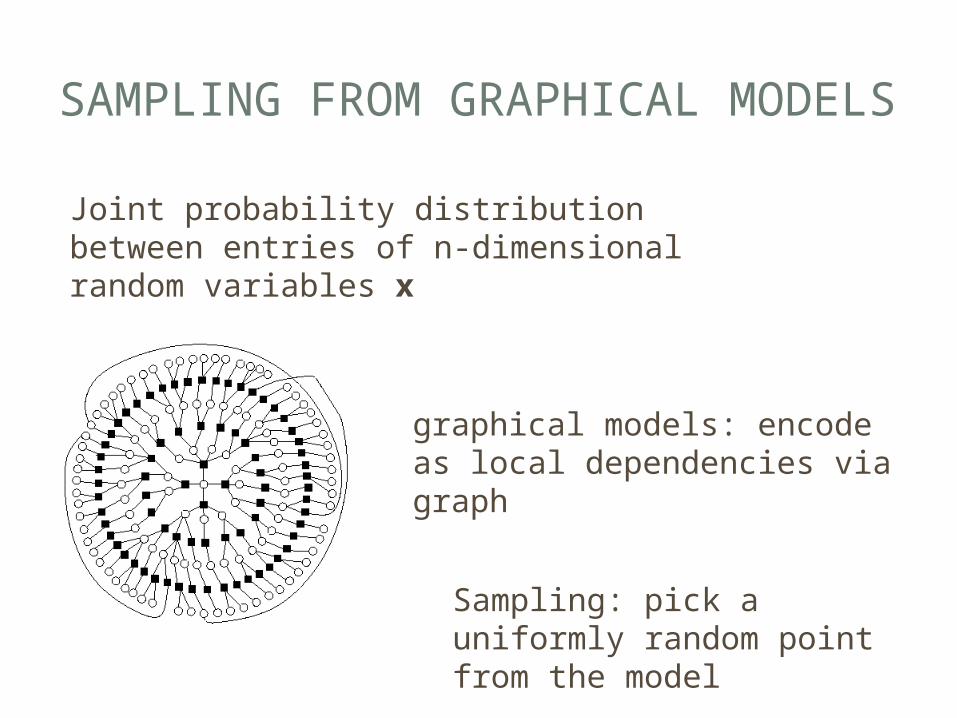
Joint probability distribution between entries of n-dimensional random variables x

graphical models: encode as local dependencies via graph

Sampling: pick a uniformly random point from the model

APPLICATIONS

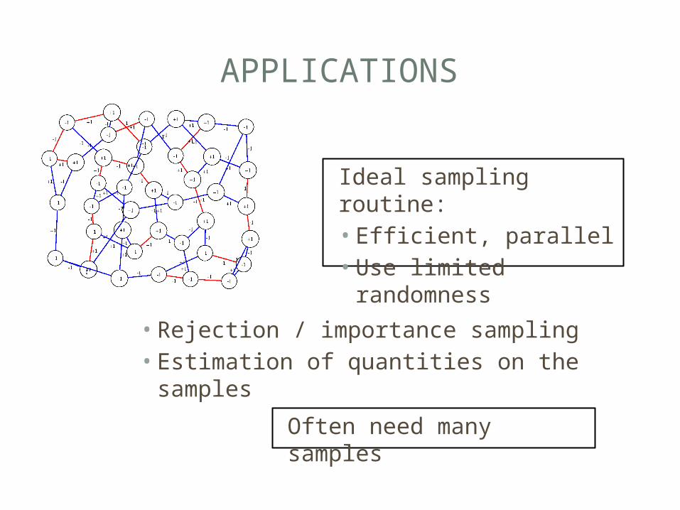
Often need many samples

• Rejection / importance sampling• Estimation of quantities on the

samples

Ideal sampling routine:• Efficient, parallel• Use limited

randomness

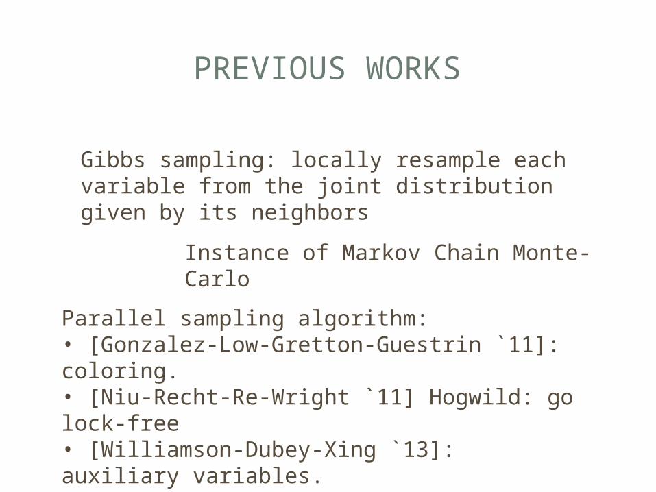
PREVIOUS WORKS

Instance of Markov Chain Monte-Carlo

Parallel sampling algorithm:• [Gonzalez-Low-Gretton-Guestrin `11]: coloring.• [Niu-Recht-Re-Wright `11] Hogwild: go lock-free• [Williamson-Dubey-Xing `13]: auxiliary variables.

Gibbs sampling: locally resample each variable from the joint distribution given by its neighbors

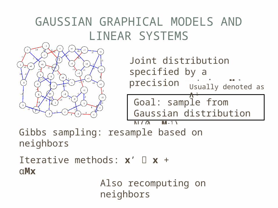
GAUSSIAN GRAPHICAL MODELS AND LINEAR SYSTEMS

Joint distribution specified by a precision matrix, M-1

Goal: sample from Gaussian distribution N(0, M-1)

Gibbs sampling: resample based on neighbors

Iterative methods: x’ x + αMx

Also recomputing on neighbors

Usually denoted as Λ-

1

CONNECTION TO SOLVING LINEAR SYSTEMS

[Johnson, Saunderson, Willsky `13]: if the precision matrix M is (generalized) diagonally dominant, then Hogwild Gibbs sampling converges

1

1

n verticesm edges

Further simplification: graph Laplacian Matrix L• Diagonal: degree• Off-diagonal:

-edge weights

2 -1 -1 -1 1 0 -1 0 1

Much more restrictive than the `graph’ in graphical models!

n rows / columnsO(m) non-zeros

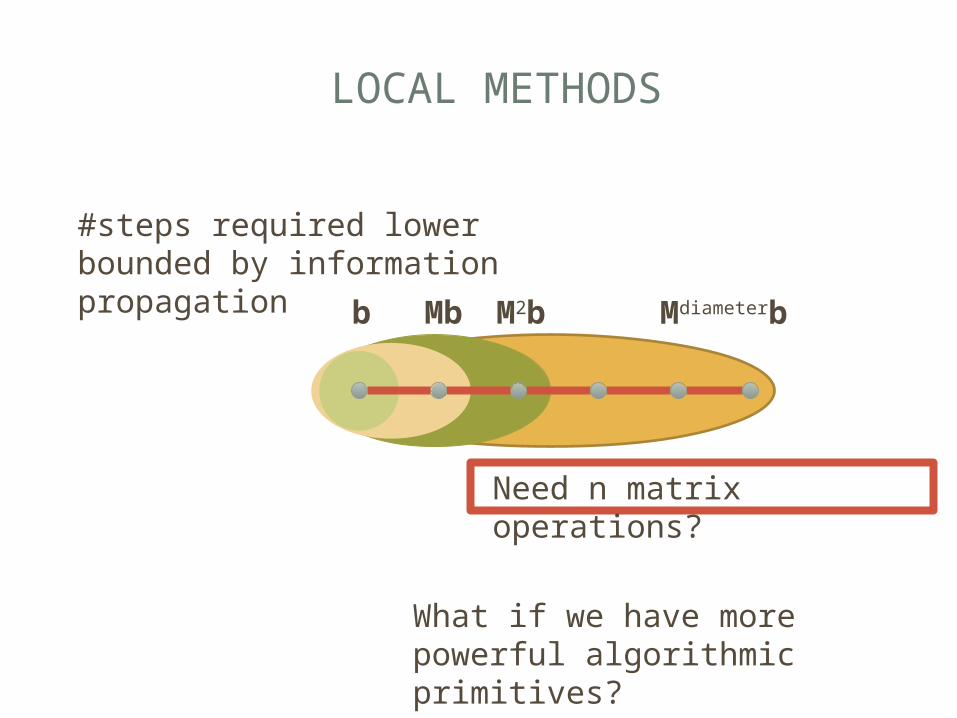
LOCAL METHODS

#steps required lower bounded by information propagation Mdiameterbb M

bM2b

Need n matrix operations?

What if we have more powerful algorithmic primitives?

ALGEBRAIC PRIMITIVE

Goal: generate random variable from the Gaussian distribution N(0, L-1)

Can generate uniform Gaussians, N(0, I)

Need: efficiently evaluable linear operator C s.t. CTC = L-

1

x ~ N(0, I), y = Cx

y ~ N(0, CTC)

Assume L is full rank for simplicity

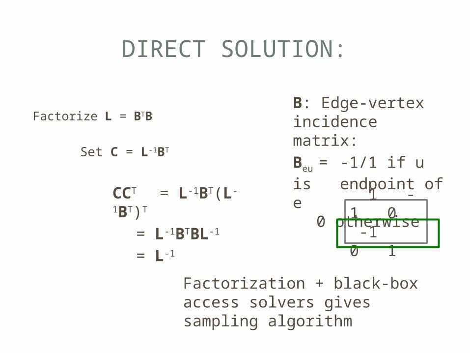
DIRECT SOLUTION:

Factorize L = BTB

Set C = L-1BT

CCT = L-1BT(L-

1BT)T

= L-1BTBL-1

= L-1

Factorization + black-box access solvers gives sampling algorithm

B: Edge-vertex incidence matrix:Beu = -1/1 if u is endpoint of e

0 otherwise 1 -1 0 -1 0 1

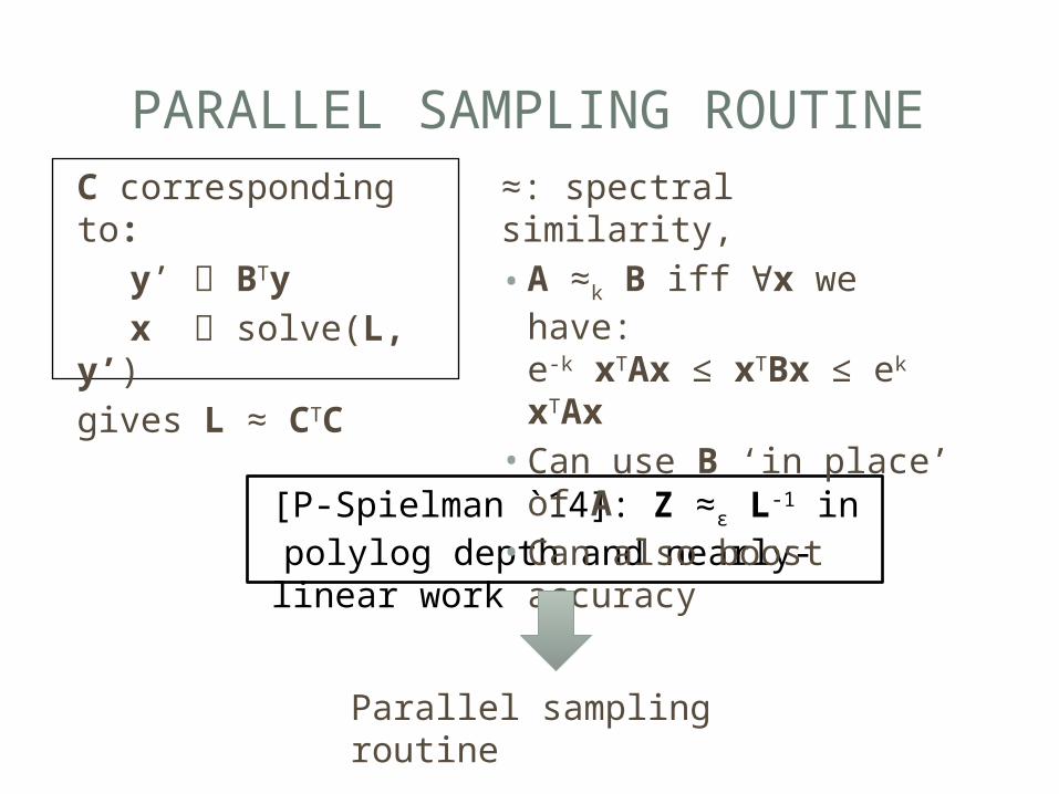
PARALLEL SAMPLING ROUTINE

[P-Spielman `14]: Z ≈ε L-1 in

polylog depth and nearly-linear work

≈: spectral similarity,• A ≈k B iff ∀x we have:

e-k xTAx ≤ xTBx ≤ ek xTAx• Can use B ‘in place’ of A• Can also boost accuracy

Parallel sampling routine

C corresponding to:y’ BTyx solve(L,

y’)gives L ≈ CTC

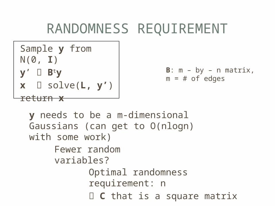
RANDOMNESS REQUIREMENTSample y from N(0, I)y’ Btyx solve(L, y’)return x

B: m – by – n matrix, m = # of edges

Optimal randomness requirement: n C that is a square matrix

Fewer random variables?

y needs to be a m-dimensional Gaussians (can get to O(nlogn) with some work)

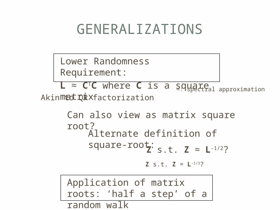
GENERALIZATIONS

Lower Randomness Requirement:L ≈ CTC where C is a square matrix

Application of matrix roots: ‘half a step’ of a random walk

Can also view as matrix square root?

Z s.t. Z ≈ L-1/2?

Z s.t. Z ≈ L-1/3?

≈: spectral approximationAkin to QR factorization

Alternate definition of square-root:

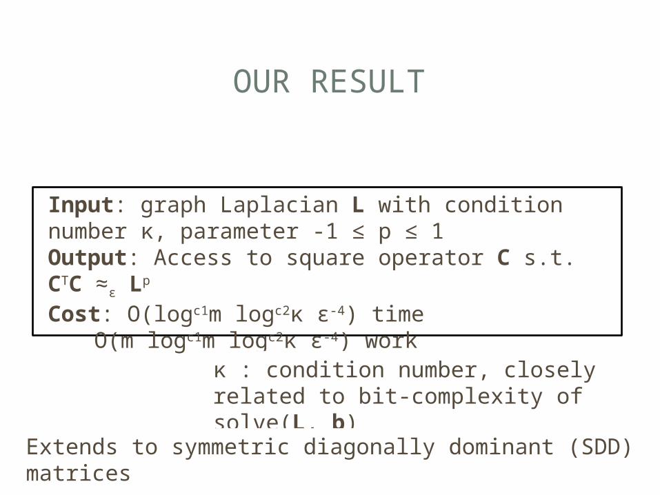
OUR RESULT

Input: graph Laplacian L with condition number κ, parameter -1 ≤ p ≤ 1Output: Access to square operator C s.t. CTC ≈ε Lp

Cost: O(logc1m logc2κ ε-4) time O(m logc1m logc2κ ε-4) work

κ : condition number, closely related to bit-complexity of solve(L, b)

Extends to symmetric diagonally dominant (SDD) matrices

SUMMARY

• Gaussian sampling closely related to linear system solves and matrix pth roots• Can approximately factor Lp into a

product of sparse matrices• Random walk polynomials can be

sparsified by sampling random walks

OUTLINE

• Gaussian sampling, linear systems, matrix-roots• Sparse factorizations of Lp

• Sparsification of random walk polynomials

SIMPLIFICATION

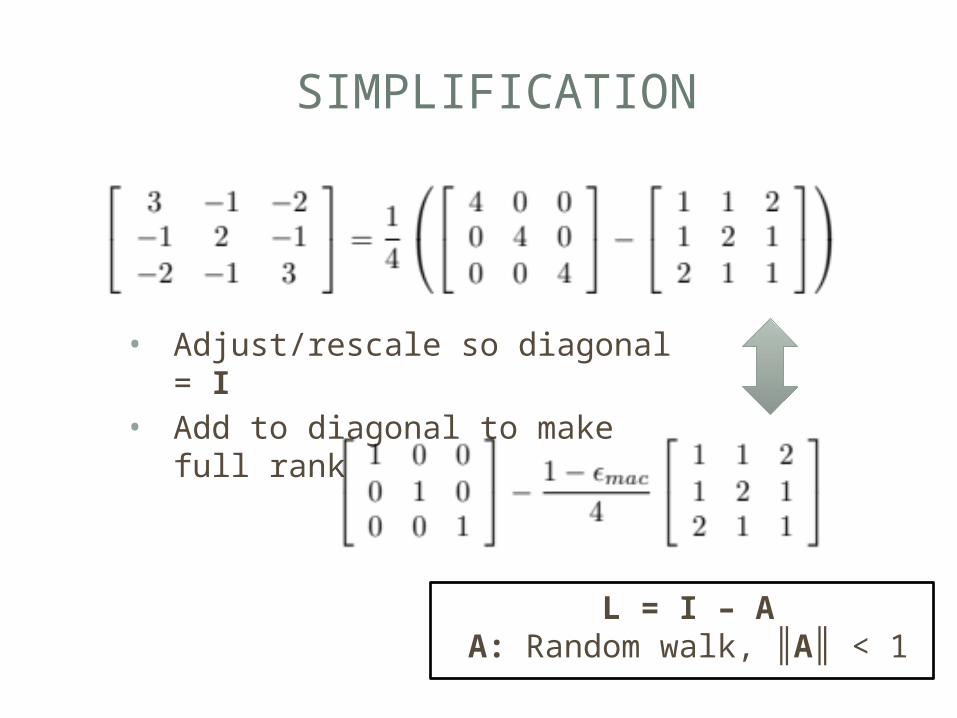
• Adjust/rescale so diagonal = I• Add to diagonal to make full rank

L = I – AA: Random walk, ║A║ < 1

PROBLEM

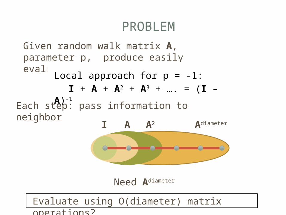
Each step: pass information to neighbor

AdiameterI A A2

Need Adiameter

Given random walk matrix A, parameter p, produce easily evaluable C s.t. CTC ≈ (I – A)p

Evaluate using O(diameter) matrix operations?

Local approach for p = -1: I + A + A2 + A3 + …. = (I –

A)-1

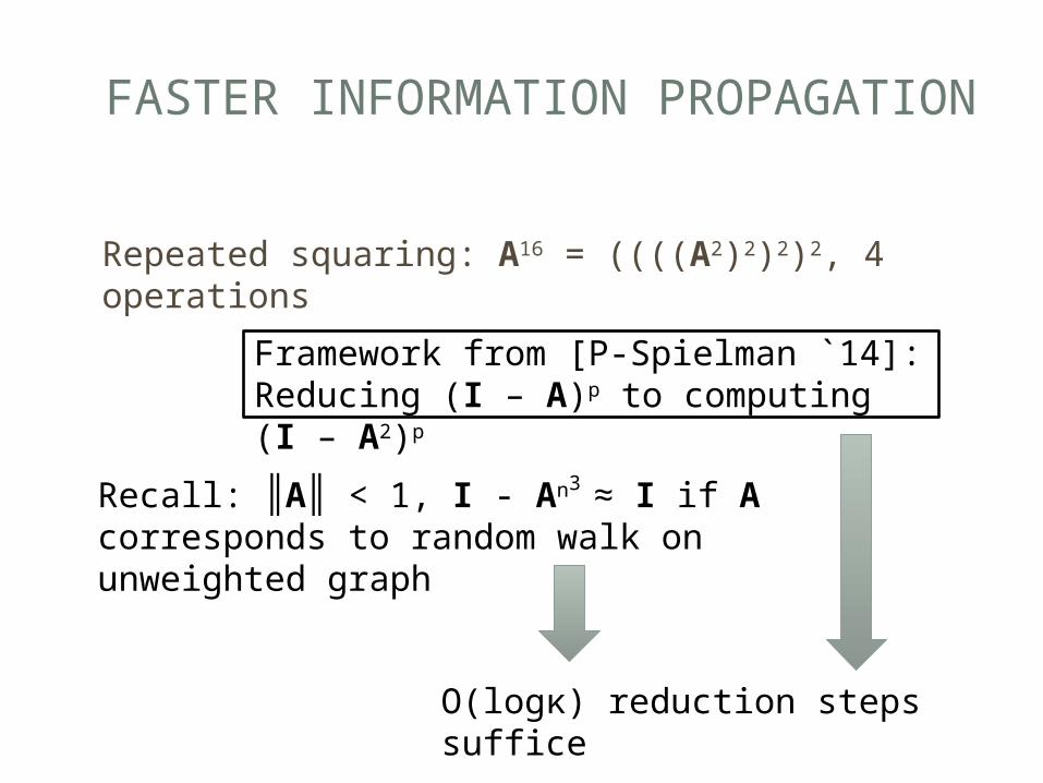
FASTER INFORMATION PROPAGATION

Recall: ║A║ < 1, I - An3 ≈ I if A corresponds to random walk on unweighted graph

Repeated squaring: A16 = ((((A2)2)2)2, 4 operations

Framework from [P-Spielman `14]:Reducing (I – A)p to computing (I – A2)p

O(logκ) reduction steps suffice

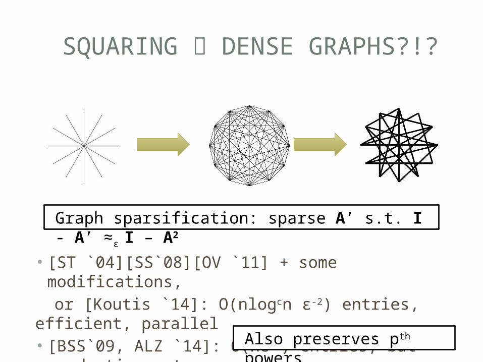
SQUARING DENSE GRAPHS?!?

• [ST `04][SS`08][OV `11] + some modifications, or [Koutis `14]: O(nlogcn ε-2) entries, efficient, parallel• [BSS`09, ALZ `14]: O(nε-2) entries, but quadratic

cost

Graph sparsification: sparse A’ s.t. I - A’ ≈ε I – A2

Also preserves pth powers

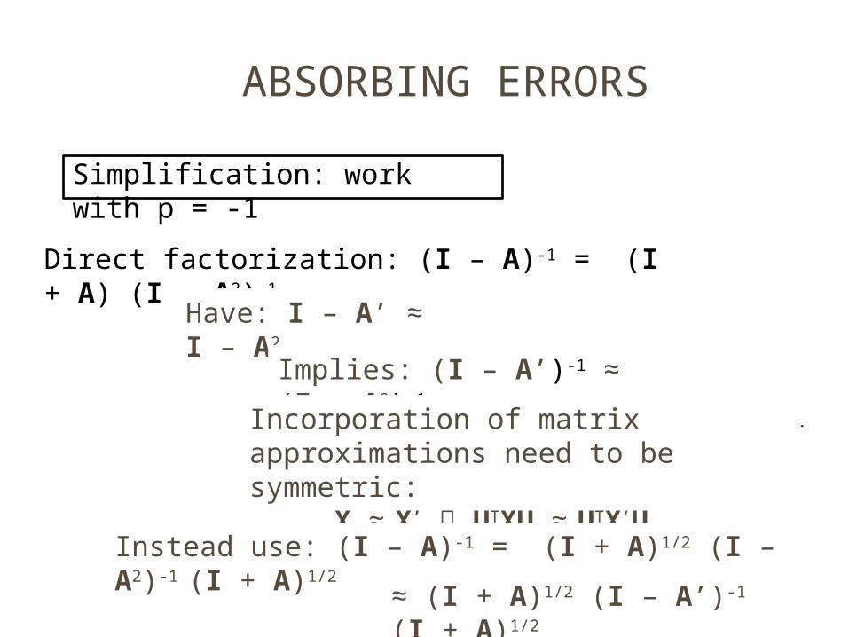
ABSORBING ERRORS

Direct factorization: (I – A)-1 = (I + A) (I – A2)-1

Simplification: work with p = -1

Have: I – A’ ≈ I – A2

Implies: (I – A’)-1 ≈ (I – A2)-

1 But NOT: (I + A) (I – A’)-1 ≈ (I + A) (I – A2)-1 Incorporation of matrix approximations need to be symmetric:

X ≈ X’ UTXU ≈ UTX’UInstead use: (I – A)-1 = (I + A)1/2 (I – A2)-1 (I + A)1/2

≈ (I + A)1/2 (I – A’)-1 (I + A)1/2

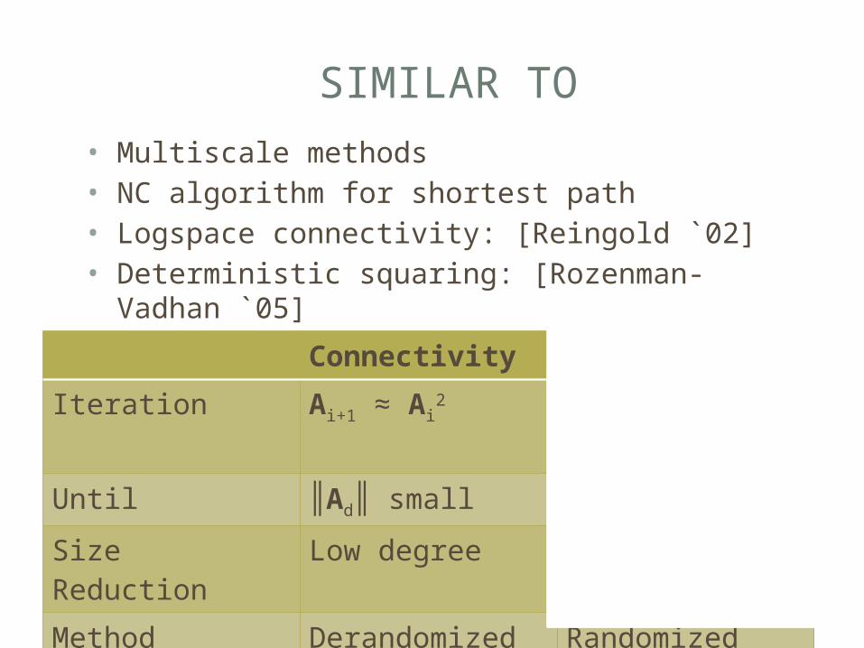
SIMILAR TO

Connectivity Our Algorithm

Iteration Ai+1 ≈ Ai2 I - Ai+1 ≈ I - Ai

2

Until ║Ad║ small ║Ad║ small

Size Reduction Low degree Sparse graph

Method Derandomized Randomized

Solution transfer

Connectivity Solution vectors

• Multiscale methods• NC algorithm for shortest path• Logspace connectivity: [Reingold `02]• Deterministic squaring: [Rozenman-Vadhan

`05]

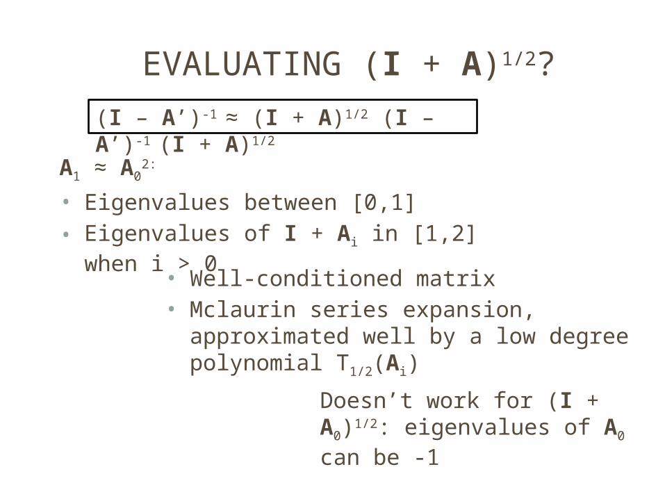
EVALUATING (I + A)1/2?

• Well-conditioned matrix• Mclaurin series expansion,

approximated well by a low degree polynomial T1/2(Ai)

A1 ≈ A02:

• Eigenvalues between [0,1]• Eigenvalues of I + Ai in [1,2] when i

> 0

Doesn’t work for (I + A0)1/2: eigenvalues of A0 can be -1

(I – A’)-1 ≈ (I + A)1/2 (I – A’)-1 (I + A)1/2

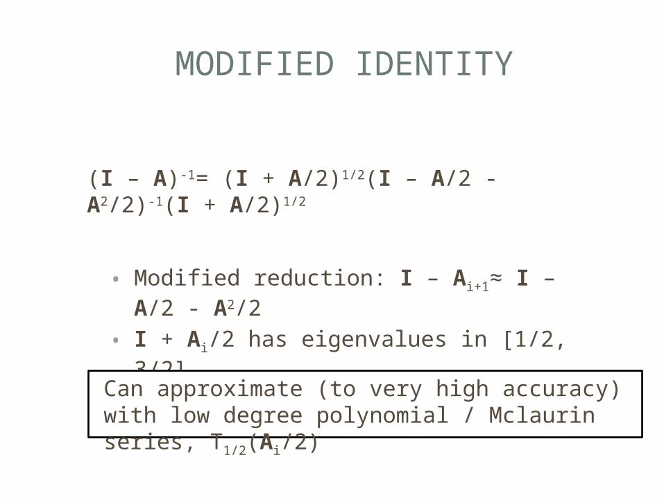
MODIFIED IDENTITY

(I – A)-1= (I + A/2)1/2(I – A/2 - A2/2)-1(I + A/2)1/2

• Modified reduction: I – Ai+1≈ I – A/2 - A2/2

• I + Ai/2 has eigenvalues in [1/2, 3/2]

Can approximate (to very high accuracy) with low degree polynomial / Mclaurin series, T1/2(Ai/2)

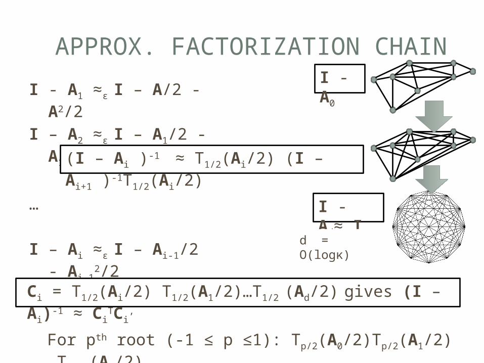
APPROX. FACTORIZATION CHAIN

For pth root (-1 ≤ p ≤1): Tp/2(A0/2)Tp/2(A1/2) …Tp/2

(Ad/2)

I - A1 ≈ε I – A/2 - A2/2

I – A2 ≈ε I – A1/2 - A12

…

I – Ai ≈ε I – Ai-1/2 - Ai-

12/2

I - Ad ≈ I

I - A0

I - Ad≈ I

d = O(logκ)

(I – Ai )-1 ≈ T1/2(Ai/2) (I – Ai+1 )-

1T1/2(Ai/2)

Ci = T1/2(Ai/2) T1/2(A1/2)…T1/2 (Ad/2) gives (I – Ai)-1 ≈ Ci

TCi,

WORKING AROUND EXPANSIONS

Alternate reduction step:

(I – A)-1 = (I + A/2) (I – 3/4 A2 -1/4 A3)-1 (I + A/2)

Composition now done with I + A/2, easy

Hard part: finding sparse approximation to I – 3/4 A2 -1/4 A3

3/4(I – A2):same as before

1/4(I – A3):cubic power

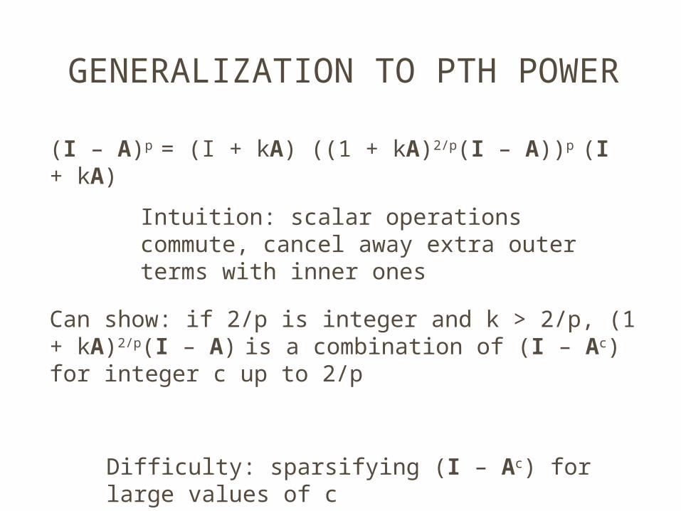
GENERALIZATION TO PTH POWER

(I – A)p = (I + kA) ((1 + kA)2/p(I – A))p (I + kA)

Intuition: scalar operations commute, cancel away extra outer terms with inner ones

Can show: if 2/p is integer and k > 2/p, (1 + kA)2/p(I – A) is a combination of (I – Ac) for integer c up to 2/p

Difficulty: sparsifying (I – Ac) for large values of c

SUMMARY

• Gaussian sampling closely related to linear system solves and matrix pth roots• Can approximately factor Lp into

a product of sparse matrices

OUTLINE

• Gaussian sampling, linear systems, matrix-roots• Sparse factorizations of Lp

• Sparsification of random walk polynomials

SPECTRAL SPARSIFICATION VIA EFFECTIVE RESISTANCE

[Spielman-Srivastava `08]: suffices to sample with probabilities at least O(logn) times weight times effective resistance

Issues: I - A3 is dense

Need to sample without explicitly generating all edges / resistances

Aka. sample with logn Auv R(u, v)

Two step approach: get sparsifier with edge count close to m, then run full sparsifier

TWO STEP APPROACH FOR I – X2

A: 1 step of random walk

A2: 2 steps of random walk

[P-Spielman `14]: for a fix midpoint, edges of A2, form a (weighted) complete graph

Replace with expanders O(mlogn) edges

Run black-box sparsifier

I - A3

A: one step of random walk

A3: 3 steps of random walk

(part of) edge uv in I - A3

Length 3 path in A: u-y-z-v

Weight: AuyAyzAzv

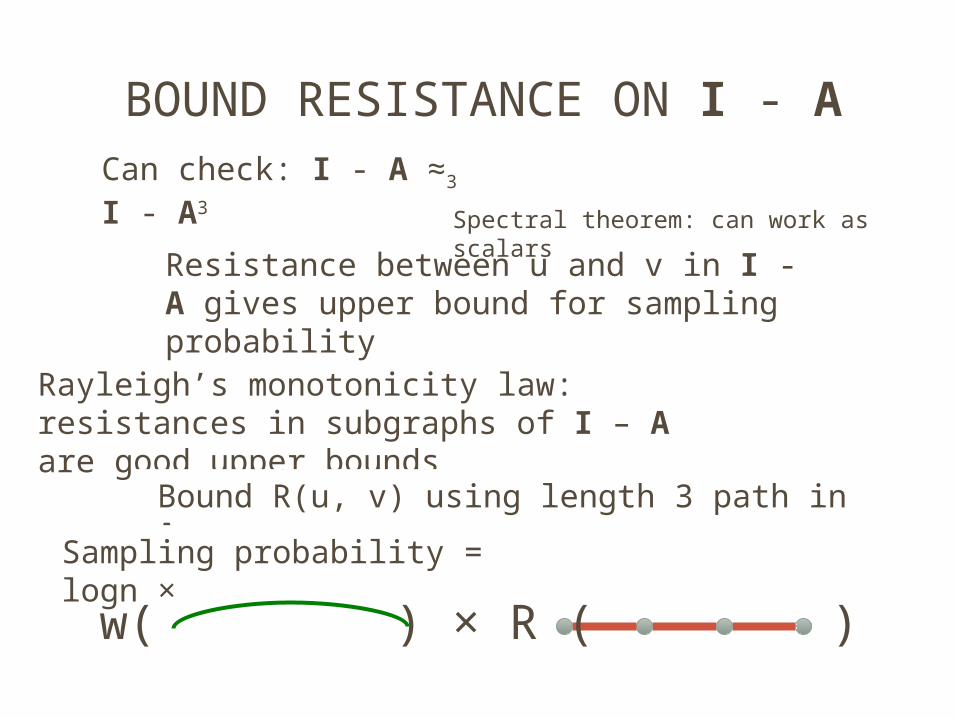
BOUND RESISTANCE ON I - A

Rayleigh’s monotonicity law: resistances in subgraphs of I – A are good upper bounds

Can check: I - A ≈3 I - A3

Resistance between u and v in I - A gives upper bound for sampling probability

Bound R(u, v) using length 3 path in A, u-y-z-v:Sampling probability = logn

×w( ) × R ( )

Spectral theorem: can work as scalars

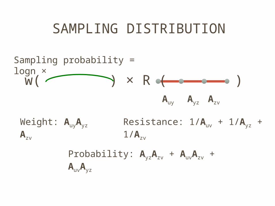
SAMPLING DISTRIBUTION

Weight: AuyAyz Azv

Probability: AyzAzv + AuvAzv +

AuvAyz

Sampling probability = logn ×

w( ) × R ( )

Resistance: 1/Auv + 1/Ayz + 1/Azv

Auy Ayz Azv

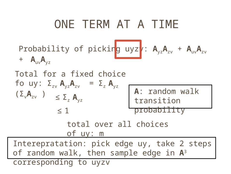
ONE TERM AT A TIME

Probability of picking uyzv: AyzAzv + AuvAzv +

AuvAyz

Interepratation: pick edge uy, take 2 steps of random walk, then sample edge in A3 corresponding to uyzv

Total for a fixed choice fo uy: Σzv AyzAzv = Σz Ayz (ΣvAzv )

A: random walk transition probability

≤ Σz Ayz

≤ 1

total over all choices of uy: m

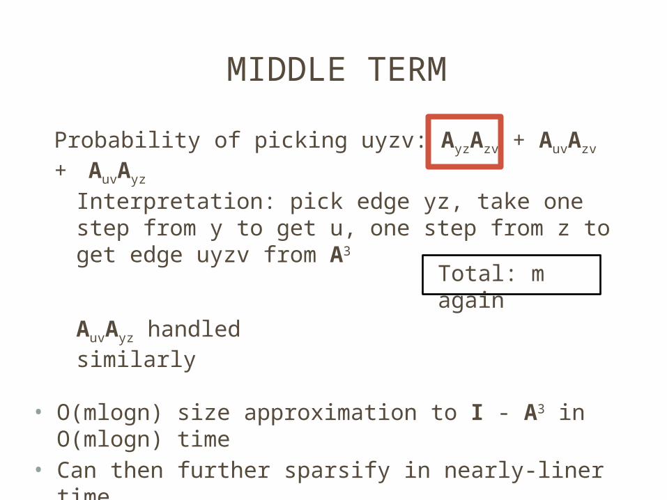
MIDDLE TERM

Interpretation: pick edge yz, take one step from y to get u, one step from z to get edge uyzv from A3

Total: m again

AuvAyz handled similarly

• O(mlogn) size approximation to I - A3 in O(mlogn) time

• Can then further sparsify in nearly-liner time

Probability of picking uyzv: AyzAzv + AuvAzv +

AuvAyz

EXTENSIONS

I - Ak in O(mklogcn) time

Even power: I – A ≈ I - A2 does not hold

But I – A2 ≈2 I - A4,

certify via 2 step matrix, same algorithm

I - Ak in O(mlogklogcn) time when k is a multiple of 4

SUMMARY

• Gaussian sampling closely related to linear system solves and matrix pth roots• Can approximately factor Lp into a

product of sparse matrices• Random walk polynomials can be

sparsified by sampling random walks

OPEN QUESTIONS

• Generalizations:• Batch sampling?• Connections to multigrid/multiscale

methods?• Other functionals of L?

• Sparsification of random walk polynomials:• Degree n polynomials in nearly-linear time?• Positive and negative coefficients?• Connections with other algorithms based on

sampling random walks?

THANK YOU!

Questions?

Manuscripts on arXiv:• http://arxiv.org/abs/1311.3286• http://arxiv.org/abs/1410.5392