runoff prediction using an integrated hybrid modelling scheme

Journal of Hydrology 372 (2009) 48–60

Contents lists available at ScienceDirect

Journal of Hydrology

journal homepage: www.elsevier .com/locate / jhydrol

Runoff prediction using an integrated hybrid modelling scheme

Renji Remesan a,*, Muhammad Ali Shamim a, Dawei Han a, Jimson Mathew b

a Water and Environmental Management Research Centre, Department of Civil Engineering, University of Bristol, Lunsford House, Cantocks Close,Clifton Bristol BS8 1UP, United Kingdomb Department of Computer Science, University of Bristol, Merchant Venture’s Building, Woodland Road, Bristol BS8 1UB, United Kingdom

a r t i c l e i n f o s u m m a r y

Article history:Received 10 May 2008Received in revised form 10 March 2009Accepted 30 March 2009

This manuscript was handled by P. Baveye,Editor-in-Chief, with the assistance ofJuan V Giraldez, Associate Editor

Keywords:Rainfall runoff modellingGamma testWaveletHybrid model

0022-1694/$ - see front matter � 2009 Elsevier B.V. Adoi:10.1016/j.jhydrol.2009.03.034

* Corresponding author. Tel.: +44 (0)117 9289768;E-mail address: [email protected] (R. Re

Rainfall runoff is a very complicated process due to its nonlinear and multidimensional dynamics, andhence difficult to model. There are several options for a modeller to consider, for example: the type ofinput data to be used, the length of model calibration (training) data and whether or not the input databe treated as signals with different frequency bands so that they can be modelled separately. This paperdescribes a new hybrid modelling scheme to answer the above mentioned questions. The proposed meth-odology is based on a hybrid model integrating wavelet transformation, a modelling engine (ArtificialNeural Network) and the Gamma Test. First, the Gamma Test is used to decide the required input datadimensions and its length. Second, the wavelet transformation decomposes the input signals into differ-ent frequency bands. Finally, a modelling engine (ANN in this study) is used to model the decomposedsignals separately. The proposed scheme was tested using the Brue catchment, Southwest England, asa case study and has produced very positive results. The hybrid model outperforms all other modelstested. This study has a wider implication in the hydrological modelling field since its general frameworkcould be applied to other model combinations (e.g., model engine could be Support Vector Machines,neuro-fuzzy systems, or even a conceptual model. The signal decomposition could be carried out by Fou-rier transformation).

� 2009 Elsevier B.V. All rights reserved.

Introduction

Rainfall–runoff dynamics is usually highly nonlinear, time-dependent and spatially varying. Significant advancements inhydrological modelling started with the introduction of unithydrograph model and its related impulse response functions(Sherman, 1932), and is considered to be the first data driven mod-el in hydrology. In the last four decades, mathematical modelling ofrainfall–runoff series, for reproducing the underlying stochasticstructure of this type of hydrological process, has been performedto a great extent. Models of AR (autoregressive) and ARMA (auto-regressive moving average) class (Box and Jenkins, 1970) haveplayed a key role in this kind of approach, producing runoff predic-tion for many different time step cases (Bartolini et al., 1988).Variant forms of these models like PAR (periodic AR), PARMA (peri-odic ARMA), DARMA (discrete ARMA) etc. were introduced withsome considerable improvements in prediction (Tao and Delleur,1976; Chang et al., 1987). Moss and Bryson (1974) introduced abivariate character to the conventional way of adopting ARX (Auto-Regressive with eXogenous input) concept in hydrological timeseries modelling. ARX and its variant form ARMAX (autoregressive

ll rights reserved.

fax: +44 (0)117 9289770.mesan).

moving average with exogenous input) were considered as muchas a success for runoff predictive tools as other models comparedin its generation (Todini, 1978). Furthermore, they are still in useeven in a plethora of new sophisticated mathematical tools(Jonsdottir et al., 2007; Karamouz et al., 2008; Young and Garnier,2006). Over the last decades, data mining techniques have beenintroduced and widely applied in hydrological studies as powerfulalternative modelling tools, such as Artificial Neural Networks(ANN) (Dawson and Wilby, 2001; Han et al., 2007a, 2007b; Brayand Han, 2004; Nayak et al., 2005, 2007), fuzzy inference system(FIS) (Zadeh, 1965; See and Openshaw, 2000; Xiong et al., 2001;Han et al., 2002; Nayak et al., 2004, 2005, 2007), and Data BasedMechanistic (DBM) models (Young, 2002; Young and Garnier,2006). A comprehensive review by ASCE Task Committee on Appli-cation of Artificial Neural Networks in Hydrology (ASCE, 2000a,b)shows the acceptance of ANN technique among hydrologists. Amajor criticism of ANN models is of their limited ability to accountfor any physics of the hydrologic processes in a catchment (Aksoyet al., 2007, 2008a,b; Koutsoyiannis, 2007). That concern is par-tially ruled out through a study by Jain et al. (2004), which provesthat the distributed structure of the ANN is able to capture certainhydrological processes such as infiltration, base flow, delayed andquick surface flow, etc. These artificial intelligent techniques exhi-bit many advantages over conventional modelling techniques,including the ability to handle enormous amounts of noisy data

mailto:[email protected]

http://www.sciencedirect.com/science/journal/00221694

http://www.elsevier.com/locate/jhydrol

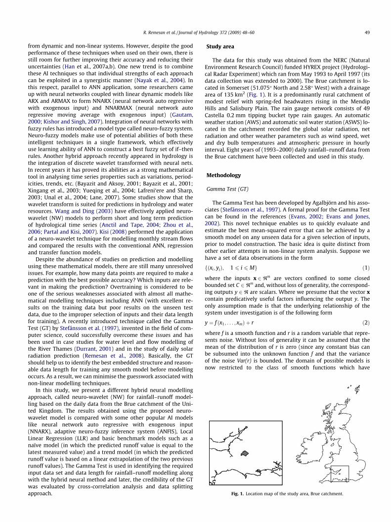
Fig. 1. Location map of the study area, Brue catchment.

R. Remesan et al. / Journal of Hydrology 372 (2009) 48–60 49

from dynamic and non-linear systems. However, despite the goodperformance of these techniques when used on their own, there isstill room for further improving their accuracy and reducing theiruncertainties (Han et al., 2007a,b). One new trend is to combinethese AI techniques so that individual strengths of each approachcan be exploited in a synergistic manner (Nayak et al., 2004). Inthis respect, parallel to ANN application, some researchers cameup with neural networks coupled with linear dynamic models likeARX and ARMAX to form NNARX (neural network auto regressivewith exogenous input) and NNARMAX (neural network autoregressive moving average with exogenous input) (Gautam,2000; Kishor and Singh, 2007). Integration of neural networks withfuzzy rules has introduced a model type called neuro-fuzzy system.Neuro-fuzzy models make use of potential abilities of both theseintelligent techniques in a single framework, which effectivelyuse learning ability of ANN to construct a best fuzzy set of if–thenrules. Another hybrid approach recently appeared in hydrology isthe integration of discrete wavelet transformed with neural nets.In recent years it has proved its abilities as a strong mathematicaltool in analysing time series properties such as variations, period-icities, trends, etc. (Bayazit and Aksoy, 2001; Bayazit et al., 2001;Xingang et al., 2003; Yueqing et al., 2004; Lafreni‘ere and Sharp,2003; Unal et al., 2004; Lane, 2007). Some studies show that thewavelet transform is suited for predictions in hydrology and waterresources. Wang and Ding (2003) have effectively applied neuro-wavelet (NW) models to perform short and long term predictionof hydrological time series (Anctil and Tape, 2004; Zhou et al.,2006; Partal and Kisi, 2007). Kisi (2008) performed the applicationof a neuro-wavelet technique for modelling monthly stream flowsand compared the results with the conventional ANN, regressionand transfer function models.

Despite the abundance of studies on prediction and modellingusing these mathematical models, there are still many unresolvedissues. For example, how many data points are required to make aprediction with the best possible accuracy? Which inputs are rele-vant in making the prediction? Overtraining is considered to beone of the serious weaknesses associated with almost all mathe-matical modelling techniques including ANN (with excellent re-sults on the training data but poor results on the unseen testdata, due to the improper selection of inputs and their data lengthfor training). A recently introduced technique called the GammaTest (GT) by Stefánsson et al. (1997), invented in the field of com-puter science, could successfully overcome these issues and hasbeen used in case studies for water level and flow modelling ofthe River Thames (Durrant, 2001) and in the study of daily solarradiation prediction (Remesan et al., 2008). Basically, the GTshould help us to identify the best embedded structure and reason-able data length for training any smooth model before modellingoccurs. As a result, we can minimise the guesswork associated withnon-linear modelling techniques.

In this study, we present a different hybrid neural modellingapproach, called neuro-wavelet (NW) for rainfall–runoff model-ling based on the daily data from the Brue catchment of the Uni-ted Kingdom. The results obtained using the proposed neuro-wavelet model is compared with some other popular AI modelslike neural network auto regressive with exogenous input(NNARX), adaptive neuro-fuzzy inference system (ANFIS), LocalLinear Regression (LLR) and basic benchmark models such as anaïve model (in which the predicted runoff value is equal to thelatest measured value) and a trend model (in which the predictedrunoff value is based on a linear extrapolation of the two previousrunoff values). The Gamma Test is used in identifying the requiredinput data set and data length for rainfall–runoff modelling alongwith the hybrid neural method and later, the credibility of the GTwas evaluated by cross-correlation analysis and data splittingapproach.

Study area

The data for this study was obtained from the NERC (NaturalEnvironment Research Council) funded HYREX project (Hydrologi-cal Radar Experiment) which ran from May 1993 to April 1997 (itsdata collection was extended to 2000). The Brue catchment is lo-cated in Somerset (51.075� North and 2.58� West) with a drainagearea of 135 km2 (Fig. 1). It is a predominantly rural catchment ofmodest relief with spring-fed headwaters rising in the MendipHills and Salisbury Plain. The rain gauge network consists of 49Castella 0.2 mm tipping bucket type rain gauges. An automaticweather station (AWS) and automatic soil water station (ASWS) lo-cated in the catchment recorded the global solar radiation, netradiation and other weather parameters such as wind speed, wetand dry bulb temperatures and atmospheric pressure in hourlyinterval. Eight years of (1993–2000) daily rainfall–runoff data fromthe Brue catchment have been collected and used in this study.

Methodology

Gamma Test (GT)

The Gamma Test has been developed by Agalbjörn and his asso-ciates (Stefánsson et al., 1997). A formal proof for the Gamma Testcan be found in the references (Evans, 2002; Evans and Jones,2002). This novel technique enables us to quickly evaluate andestimate the best mean-squared error that can be achieved by asmooth model on any unseen data for a given selection of inputs,prior to model construction. The basic idea is quite distinct fromother earlier attempts in non-linear system analysis. Suppose wehave a set of data observations in the form

fðxi; yiÞ; 1 6 i 6 Mg ð1Þ

where the inputs x 2 Rm are vectors confined to some closedbounded set C 2 Rm and, without loss of generality, the correspond-ing outputs y 2 R are scalars. Where we presume that the vector xcontain predicatively useful factors influencing the output y. Theonly assumption made is that the underlying relationship of thesystem under investigation is of the following form

y ¼ f ðx1; . . . ; xmÞ þ r ð2Þ

where f is a smooth function and r is a random variable that repre-sents noise. Without loss of generality it can be assumed that themean of the distribution of r is zero (since any constant bias canbe subsumed into the unknown function f and that the varianceof the noise Var(r) is bounded. The domain of possible models isnow restricted to the class of smooth functions which have

50 R. Remesan et al. / Journal of Hydrology 372 (2009) 48–60

bounded first partial derivatives. The gamma statistic (C) is the esti-mate of that part of the variance of the output that cannot be ac-counted for by a smooth data model.

The Gamma Test is based on N [i, k], which are the kth(1 6 k 6 p) nearest neighbours xN[1, k] (1 6 k 6 p) for each vectorxi (1 6 k 6 p). Specifically; the Gamma Test is derived from the Del-ta function of input vectors:

dMðkÞ ¼1M

XM

i¼1

jxNð1;kÞ � xij2 ð1 6 k 6 pÞ ð3Þ

where |. . .| denotes Euclidean distance, and corresponding Gammafunction of output values:

cMðkÞ ¼1

2M

XM

i¼1

jyNð1;kÞ � yij2 ð1 6 k 6 pÞ ð4Þ

where yN(1, k) is the corresponding y-value for the kth nearest neigh-bour of xi in (3). In order to compute C a least squares fitted regres-sion line is constructed for the p points (dM(k), cM(k))

c ¼ Adþ C ð5Þ

The intercept on the vertical (d = 0) axis is the C value, as it can beshown as

cMðkÞ ! VarðrÞ in probability as dMðkÞ ! 0 ð6Þ

The graphical output of this regression line (5) can provide veryuseful information for hydrological modellers. First, it is remarkablethat the vertical intercept C of y axis offers an estimate of the bestMSE achievable utilising a modelling technique for unknownsmooth functions of continuous variables (Evans and Jones, 2002).Second, the gradient A offers an indication of model’s complexity(a steeper gradient indicates a model of greater complexity).

Another term associated with the Gamma Test is Vratio. A Vratio

close to zero indicates that there is a high degree of predictabilityof the given output y. We can also determine the reliability of thegamma statistic by running a series of the Gamma Test for increas-ing M, to establish the size of data set required to produce a stableasymptote. This is known as the M-test. M-test and its result wouldhelp us to avoid wasteful attempts in fitting the model beyond thestage where the MSE on the training data is smaller than Var(r),which may lead to overfitting. The M-test also helps us to decidehow much data is required to build a model with a mean-squarederror which approximates the estimated noise variance.

Local Linear Regression (LLR) model

The Local Linear Regression model is a popular nonparametricregression technique which has been widely used in many lowdimensional forecasting and smoothing problems. Reliable model-ling even on a small amount of sample data and accurate predic-tions in regions of high data density in the input space areconsidered as the major advantages of LLR models. The LLR proce-dure requires only three data points to obtain an initial predictionand then uses all newly updated data in the order they becomesavailable to make further predictions. Deciding the size of pmax,(the number of near neighbours to be included for the local linearmodelling) is the tricky part in LLR modelling.

Given a neighbourhood of pmax points, we must solve a linearmatrix equation

Xm ¼ y ð7Þ

where X is a pmax � d matrix of the pmax input points in d-dimen-sions, xi (1 6 i 6 pmax) are the nearest neighbour points, y is a col-umn vector of length pmax of the corresponding outputs, and m isa column vector of parameters that must be determined to providethe optimal mapping from X to y, such that

x11 x12 x13 . . . x1d

x21 x22 x23 . . . x2d

..

. ... ..

. . .. ..

.

xxp max1 xxp max2 xxp max3 � � � xxp maxd

0BBBB@

1CCCCA

m1

m2

m3

..

.

md

0BBBBBBB@

1CCCCCCCA¼

y1

y1

..

.

yp max

0BBBB@

1CCCCA ð8Þ

The rank r of the matrix X is the number of linearly independentrows, which will affect the existence or uniqueness of the solutionfor m.

If the matrix X is square and non-singular then a unique solu-tion to Eq. (7) is m = X�1y. If X is not square or singular, we shouldfind a vector m which minimises

jXm� yj2 ð9Þ

where the unique solution to this problem is provided by m = Xywhere X is a pseudo-inverse matrix.

Neural network autoregressive with exogenous inputs (NNARX) model

In this study, a Neural Network Autoregressive with ExogenousInputs (NNARX) model is built on the basis of a linear ARX-model.The discrete linear ARX model can be expressed as a simple lineardifference equation. A simple linear ARX model for rainfall–runoffmodelling with one exogenous input (rainfall) can be expressed asfollows:

QðtÞ ¼ �Xna

n¼1

anQðt � nÞ þXnb

m¼1

bmPðt �mÞ þ eðtÞ ð10Þ

where Q is the runoff, t represents time step, an, and bm denote themodel parameters, na and nb are the orders associated with the out-put (Q) and the input (P), e(t) is the mapping error. The choice of theappropriate ARX model structure (the appropriate na and nb) is veryimportant; these can be guided with Akaike’s Information Criterion(AIC) and the best input combination selection is selected by theGamma Test. In this study we established a three-layer feed for-ward neural network (one input layer, one hidden layer and oneoutput layer). This topology has proved its ability in modellingmany real-world functional problems. The selection of hidden neu-rons is the tricky part in ANN modelling as it relates to the complex-ity of the system being modelled and there are several ways ofdoing it, such as the geometric average between input and outputvectors dimension (Maren et al., 1990), is the same as the numberof inputs used for the modelling (Mechaqrane and Zouak, 2004),set to be twice the input layer dimension plus one (Hecht-Nielsen,1990), etc. In this study, the Hecht-Nielsen (1990) approach hasbeen adopted according to our past experience with it. The Leven-berg–Marquardt training algorithm was used in this study to adjustthe weights of the feed forward neural network.

Adaptive neuro-fuzzy inference system (ANFIS)

This is a well known artificial intelligence technique that hasbeen used in modelling hydrological processes. The ability of neu-ral network to learn fuzzy structure from the input–output datasets in an interactive manner has encouraged many researchersto combine the ANN and the fuzzy logic effectively to organize net-work structure itself and to adapt parameters of a fuzzy system.Several well-known neuro-fuzzy modelling algorithms are avail-able in the literature, such as fuzzy inference networks, fuzzyaggregation networks, neural network-driven fuzzy reasoning, fuz-zy modelling networks, fuzzy associative memory systems etc.(Keller et al., 1992; Horikawa et al., 1992; Kosko, 1992). The adap-tive neuro-fuzzy inference system (ANFIS), proposed by Prof. J.S.Roger Jang of National Tsing Hua University, is based on the first-order Sugeno fuzzy model.


For simplicity, the fuzzy inference system with two fuzzy If/Then rules can be expressed as follows. For a first-order Sugenofuzzy model, a typical rule set with two fuzzy If/Then rules canbe expressed as

Rule 1 : If x is A1 and y is B1 Then f 1 ¼ p1xþ q1yþ r1 ð11ÞRule 2 : If x is A2 and y is B2 Then f 2 ¼ p2xþ q2yþ r2 ð12Þ

where, x and y are the crisp inputs to the node i, Ai and Bi are thelinguistic labels (low, medium, high, etc.) characterized by conve-nient membership functions and pi, qi and ri are the consequenceparameters (i = 1 or 2). The corresponding equivalent ANFIS archi-tecture can be found in Fig. 2. In the ANFIS, nodes in the same layerhave similar functions as described below:

Layer 1 (Input nodes)Nodes of this layer generates membership grades of the crisp

inputs which belong to each of the convenient fuzzy sets usingthe membership functions. The generated bell-shaped member-ship function given below was used:

lAiðxÞ ¼ 1

1þ ððx� ciÞ=aiÞ2bið13Þ

where lAiis the appropriate membership function for Ai fuzzy set,

and {ai, bi, ci} is the membership function’s parameter set (premiseparameters) that changes the shape of membership function from1 to 0.

Layer 2 (rule nodes)In this layer, the rule operator (AND/OR) is applied to get one

output that represents the results of the antecedent for a fuzzyrule. The outputs of the second layer, called as firing strengthsO2

i , are the products of the incoming signals obtained from thelayer 1, named as w below:

O2i ¼ wi ¼ lAi

ðxÞlBiðyÞ i ¼ 1;2 ð14Þ

Layer 3 (average nodes)In this layer, the nodes calculate the ratio of the ith rule’s firing

strength to the sum of all rules’ firing strengths

O3i ¼ �wi ¼

wiPiwi

i ¼ 1;2 ð15Þ

Layer 4 (consequent nodes)In this layer, the contribution of ith rule towards the total out-

put or the model output and/or the function calculated as follows:

O4i ¼ �wifi ¼ �wiðpixþ qiyþ riÞ i ¼ 1;2 ð16Þ

Fig. 2. The basic structure of the ANFIS.

where, �wi is the output of Layer 3 and {pi, qi, ri} are the coefficientsof a linear combination in Sugeno inference system. These parame-ters of this layer are referred to as consequent parameters.

Layer 5 (output nodes)This layer is called as the output nodes. This layer’s single fixed

node computes the final output as the summation of all incomingsignals.

O5i ¼ f ðx; yÞ ¼

PiwifiPiwi

ð17Þ

The learning algorithm for ANFIS is a hybrid algorithm, which is acombination between the gradient descent method and the leastsquares method for identifying nonlinear input parameters {ai, bi, ci}and the linear output parameters {pi, qi, ri}, respectively. The ANFISmodelling was performed using the ‘‘subtractive fuzzy clustering”function due to its good performance with a small number of rules.Further detailed information of ANFIS can be found in Jang (1993).

Neuro-wavelet (NW) model

The wavelet was introduced by Morlet and Grossman (1984) asa time-scale analysis tool for non-stationary signals for analysingirregular data with discontinuities and non-linearity. The wavelettransform could be used as a tool to split up data or functions intodifferent frequency components, and then one could study eachcomponent with a certain resolution. Flexibility is the key advan-tage of wavelets over Fourier analysis; this helps us to study thesignal of interest at various resolutions. Fourier transform tech-niques are widely used for linear decomposition of static time ser-ies. The problem with Fourier approach is that information in agiven time series is represented as a function of frequency withno specific time information. On the other hand, a wavelet analysisworks with translation and dilation of a single local function w,generally referred to as mother wavelet. In other words, the advan-tage of wavelet transform is that the wavelet coefficient reflects ina simple and precise manner the properties of the underlying func-tion. Wavelet transform theory and its application to multi-resolu-tion signal decomposition has been thoroughly developed and welldocumented over the past decades (Daubechies, 1988, 1992).Daubechies (1988) introduced the concept of orthogonal wavelet;generally referred to as Daybecies wavelet. Indeed, multi-resolu-tion analysis and discrete wavelet transform have a strong poten-tial for exploring various dynamic features of any time dependentdata.

In an orthonormal multi-resolution analysis, a signal, f(t)eV�1, isdecomposed into an infinite series of detail functions, gi(t), suchthat, f ðtÞ ¼

P10 giðtÞ. The first level decomposition is done by pro-

jecting onto two orthogonal subspaces, V0 and W0, whereV�1 = V0 �W0 and � are the direct sum operator. The projectionproduces f0(t)eV0, a low resolution approximation of f(t) andg0(t)eW0, the detail lost in going from f(t) ? f0(t). The decomposi-tion continues by projecting f0(t) onto V1 and W1 and so on. Theorthonormal bases of Vj and Wj are given by,

wj;k ¼ 2�j=2wð2�jx� kÞ ð18Þ/j;k ¼ 2�j=2wð2�jx� kÞ ð19Þ

where w(t) is the mother wavelet and u(t) is the scaling function(Daubechies, 1992) whereZ

wðxÞdt ¼ 0() wð0Þ ¼ 0 ð20ÞZ

/ðxÞdt ¼ 1() /ð1Þ ¼ 1 ð21Þ


w(w) and u(w) are the Fourier transform of u(t) and w(t), respec-tively. The projection equations are

giðtÞ ¼X1k�1

djk2�ðj=2Þwð2�jt � kÞ ð22Þ

djk ¼ hfj�1ðtÞ;wj;ki ð23Þ

fiðtÞ ¼X1k�1

cjk2�ðj=2Þwð2�jt � kÞ ð24Þ

cjk ¼ hfj�1ðtÞ;/j;ki ð25Þ

where djk and cj

k are the projection coefficients and h.,.i is the L2 In-ner product. The nested sequence of subspaces, Vj constitutes themulti-resolution analysis. Conditions for the multiresolution to beorthonormal are 1) wj,k and uj,k must be orthonormal bases of Vj

and Wj, respectively, (2) Wj \ Wk, for j – k; and (3) Wj \ Vj, whichleads to the following conditions on w and u.

h/j;k;/j;mi ¼ dk;m ð26Þh/j;k;wj;mi ¼ 0 ð27Þhwj;k;wl;mi ¼ dj;l:dk;m ð28Þ

Since u(t) e V0 � V�1 and w(t) e W0 � V�1, they can be representedas linear combinations of the basis of V�1

/ðtÞ ¼ 2X1k�1

hk/ð2t � kÞ ð29Þ

wðtÞ ¼ 2X1k�1

gk/ð2t � kÞ ð30Þ

In frequency domain Eqs. (26) and (27) become

/ðwÞ ¼ Hw2

� �/

w2

� �ð31Þ

wðwÞ ¼ Gw2

� �/

w2

� �ð32Þ

For multi-resolution analysis, the sequences hk and gk in the aboveequations represent the impulse responses of filters. In this paperwe use the above multi resolution data in the prediction model. Gi-ven a signal f(t) of length N, the DWT consists of log 2N stages atmost. The first step produces, starting from f(t), two sets of coeffi-cients: approximation coefficients A1, and detail coefficients D1.These vectors are obtained by convolving f(t) with the low-pass fil-ter h1 for approximation, and with the high-pass filter g1 for the de-tail. The next step splits the approximation coefficients A1 into twoparts using the same scheme (h2 and g2), replacing f(x) by A1, andproducing A2 and D2, and so on. In other words, we wish to build amulti resolution representation based on the differences of informa-tion available at two successive resolutions 2J and 2J + 1.

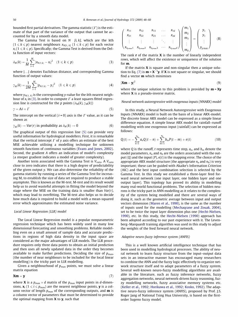
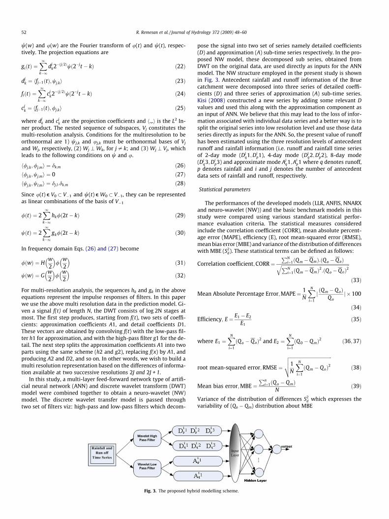
In this study, a multi-layer feed-forward network type of artifi-cial neural network (ANN) and discrete wavelet transform (DWT)model were combined together to obtain a neuro-wavelet (NW)model. The discrete wavelet transfer model is passed throughtwo set of filters viz: high-pass and low-pass filters which decom-

Fig. 3. The proposed hybr

pose the signal into two set of series namely detailed coefficients(D) and approximation (A) sub-time series respectively. In the pro-posed NW model, these decomposed sub series, obtained fromDWT on the original data, are used directly as inputs for the ANNmodel. The NW structure employed in the present study is shownin Fig. 3. Antecedent rainfall and runoff information of the Bruecatchment were decomposed into three series of detailed coeffi-cients (D) and three series of approximation (A) sub-time series.Kisi (2008) constructed a new series by adding some relevant Dvalues and used this along with the approximation component asan input of ANN. We believe that this may lead to the loss of infor-mation associated with individual data series and a better way is tosplit the original series into low resolution level and use those dataseries directly as inputs for the ANN. So, the present value of runoffhas been estimated using the three resolution levels of antecedentrunoff and rainfall information (i.e. runoff and rainfall time seriesof 2-day mode (Dj

q1;Dip1), 4-day mode (Dj

q2;Dip2), 8-day mode

(Djq3;Di

p3) and approximate mode Ajq1;Ai

p1 where q denotes runoff,p denotes rainfall and i and j denotes the number of antecedentdata sets of rainfall and runoff, respectively.

Statistical parameters

The performances of the developed models (LLR, ANFIS, NNARXand neuro-wavelet (NW)) and the basic benchmark models in thisstudy were compared using various standard statistical perfor-mance evaluation criteria. The statistical measures consideredinclude the correlation coefficient (CORR), mean absolute percent-age error (MAPE), efficiency (E), root mean-squared error (RMSE),mean bias error (MBE) and variance of the distribution of differenceswith MBE (S2

d). These statistical terms can be defined as follows:

Correlation coefficient;CORR ¼PN

i¼1ðQm �QmÞ:ðQ o �Q oÞffiffiffiffiffiffiffiffiffiffiffiffiffiffiffiffiffiffiffiffiffiffiffiffiffiffiffiffiffiffiffiffiffiffiffiffiffiffiffiffiffiffiffiffiffiffiffiffiffiffiffiffiffiffiffiffiffiffiffiffiPNi¼1ðQm �QmÞ2:ðQ o �QoÞ2

q

ð33Þ

Mean Absolute Percentage Error;MAPE ¼ 1N

XN

i¼1

j ðQ m �Q oÞQ o

j � 100

ð34Þ

Efficiency; E ¼ E1 � E2

E1ð35Þ

where E1 ¼XN

i¼1

ðQ o � Q oÞ2 and E2 ¼XN

i¼1

ðQ 0 � Q mÞ2 ð36;37Þ

root mean-squared error;RMSE ¼

ffiffiffiffiffiffiffiffiffiffiffiffiffiffiffiffiffiffiffiffiffiffiffiffiffiffiffiffiffiffiffiffiffiffiffiffiffi1N

XN

i¼1

ðQm � QoÞ2vuut ð38Þ

Mean bias error;MBE ¼Pn

i¼1ðQ o � Q mÞN

ð39Þ

Variance of the distribution of differences S2d which expresses the

variability of (Qo � Qm) distribution about MBE

id modelling scheme.

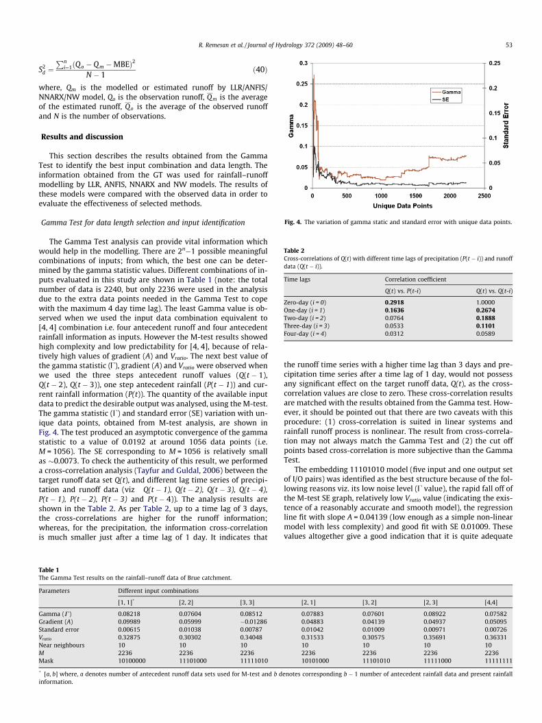
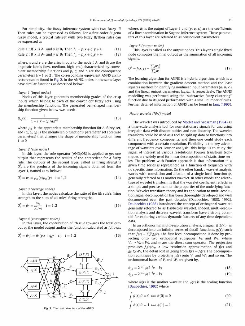
Fig. 4. The variation of gamma static and standard error with unique data points.

Table 2Cross-correlations of Q(t) with different time lags of precipitation (P(t � i)) and runoffdata (Q(t � i)).

Time lags Correlation coefficient

Q(t) vs. P(t-i) Q(t) vs. Q(t-i)

Zero-day (i = 0) 0.2918 1.0000One-day (i = 1) 0.1636 0.2674Two-day (i = 2) 0.0764 0.1888Three-day (i = 3) 0.0533 0.1101Four-day (i = 4) 0.0312 0.0589


S2d ¼

Pni¼1ðQo � Qm �MBEÞ2

N � 1ð40Þ

where, Qm is the modelled or estimated runoff by LLR/ANFIS/NNARX/NW model, Qo is the observation runoff, Qm is the averageof the estimated runoff, Qo is the average of the observed runoffand N is the number of observations.

Results and discussion

This section describes the results obtained from the GammaTest to identify the best input combination and data length. Theinformation obtained from the GT was used for rainfall–runoffmodelling by LLR, ANFIS, NNARX and NW models. The results ofthese models were compared with the observed data in order toevaluate the effectiveness of selected methods.

Gamma Test for data length selection and input identification

The Gamma Test analysis can provide vital information whichwould help in the modelling. There are 2n�1 possible meaningfulcombinations of inputs; from which, the best one can be deter-mined by the gamma statistic values. Different combinations of in-puts evaluated in this study are shown in Table 1 (note: the totalnumber of data is 2240, but only 2236 were used in the analysisdue to the extra data points needed in the Gamma Test to copewith the maximum 4 day time lag). The least Gamma value is ob-served when we used the input data combination equivalent to[4, 4] combination i.e. four antecedent runoff and four antecedentrainfall information as inputs. However the M-test results showedhigh complexity and low predictability for [4, 4], because of rela-tively high values of gradient (A) and Vratio. The next best value ofthe gamma statistic (U), gradient (A) and Vratio were observed whenwe used the three steps antecedent runoff values (Q(t � 1),Q(t � 2), Q(t � 3)), one step antecedent rainfall (P(t � 1)) and cur-rent rainfall information (P(t)). The quantity of the available inputdata to predict the desirable output was analysed, using the M-test.The gamma statistic (U) and standard error (SE) variation with un-ique data points, obtained from M-test analysis, are shown inFig. 4. The test produced an asymptotic convergence of the gammastatistic to a value of 0.0192 at around 1056 data points (i.e.M = 1056). The SE corresponding to M = 1056 is relatively smallas �0.0073. To check the authenticity of this result, we performeda cross-correlation analysis (Tayfur and Guldal, 2006) between thetarget runoff data set Q(t), and different lag time series of precipi-tation and runoff data (viz Q(t � 1), Q(t � 2), Q(t � 3), Q(t � 4),P(t � 1), P(t � 2), P(t � 3) and P(t � 4)). The analysis results areshown in the Table 2. As per Table 2, up to a time lag of 3 days,the cross-correlations are higher for the runoff information;whereas, for the precipitation, the information cross-correlationis much smaller just after a time lag of 1 day. It indicates that

Table 1The Gamma Test results on the rainfall–runoff data of Brue catchment.

Parameters Different input combinations

[1, 1]* [2, 2] [3, 3]

Gamma (C) 0.08218 0.07604 0.08512Gradient (A) 0.09989 0.05999 �0.01286Standard error 0.00615 0.01038 0.00787Vratio 0.32875 0.30302 0.34048Near neighbours 10 10 10M 2236 2236 2236Mask 10100000 11101000 11111010

* [a, b] where, a denotes number of antecedent runoff data sets used for M-test and b dinformation.

the runoff time series with a higher time lag than 3 days and pre-cipitation time series after a time lag of 1 day, would not possessany significant effect on the target runoff data, Q(t), as the cross-correlation values are close to zero. These cross-correlation resultsare matched with the results obtained from the Gamma test. How-ever, it should be pointed out that there are two caveats with thisprocedure: (1) cross-correlation is suited in linear systems andrainfall runoff process is nonlinear. The result from cross-correla-tion may not always match the Gamma Test and (2) the cut offpoints based cross-correlation is more subjective than the GammaTest.

The embedding 11101010 model (five input and one output setof I/O pairs) was identified as the best structure because of the fol-lowing reasons viz. its low noise level (U value), the rapid fall off ofthe M-test SE graph, relatively low Vratio value (indicating the exis-tence of a reasonably accurate and smooth model), the regressionline fit with slope A = 0.04139 (low enough as a simple non-linearmodel with less complexity) and good fit with SE 0.01009. Thesevalues altogether give a good indication that it is quite adequate

[2, 1] [3, 2] [2, 3] [4,4]

0.07883 0.07601 0.08922 0.075820.04883 0.04139 0.04937 0.050950.01042 0.01009 0.00971 0.007260.31533 0.30575 0.35691 0.3633110 10 10 102236 2236 2236 223610101000 11101010 11111000 11111111

enotes corresponding b � 1 number of antecedent rainfall data and present rainfall


to construct a nonlinear predictive model using around 1056 datapoints and remaining data out of total 2240 data points were usedas the validation data set. To confirm the reliability of this result,data partitioning approach was adopted (Tayfur and Guldal,2006). Different scenarios of data partitioning into training andtesting periods were tried in order to see the optimal length oftraining data required for modelling with out overfitting duringtraining. Overfitting occurs because of large number of parametersand training data length, which lead to a precise fit memorising theset of training data and thereby loose generalization and poor val-idation results. The Table 3 shows different partitioning scenariosand the related CORR and RMSE values for each scenario duringtraining and validation using neuro-wavelet (NW) model. The ma-jor statistical parameter values for the training and testing periodsfor each scenario in Table 3 is presented in the Table 4. As per Table3, best RMSE is obtained for scenario 6 with value of 0.429 m3/swhere 1500 data points were used in the training. With the train-ing results alone, one can observe that employing more than 750data points in the training period would results in satisfactory run-off prediction with higher CORR values. In the same time we canobserve a reduction in statistical term values (higher RMSE and

Table 3Different data partitioning scenarios into training and testing periods and their modelling

Scenarios Training data length Training period

CORR

Case 1 250 0.608Case 2 500 0.897Case 3 750 0.924Case 4 1000 0.964Case 5 1100 0.966Case 6 1250 0.973Case 7 1500 0.975Case 8 1750 0.953Case 9 2000 0.950

Table 4Major statistical parameters for precipitation (mm/day) and runoff (m3/s) for the scenario

Scenarios Training phase

Precipitation data (mm) Runoff data (m3/s)

Xmax Xmin Xmean Xmax Xmin Xm

Case 1 22.54 0 2.74 29.44 0.247 2.8Case 2 35.27 0 2.90 29.44 0.222 2.9Case 3 35.27 0 2.65 29.44 0.167 2.2Case 4 35.27 0 2.45 29.44 0.167 2.0Case 5 35.27 0 2.44 29.44 0.164 1.9Case 6 35.27 0 2.26 29.44 0.164 1.9Case 7 35.27 0 2.33 29.44 0.164 1.8Case 8 35.27 0 2.37 32.07 0.164 1.9Case 9 35.27 0 2.34 32.07 0.164 1.9

Table 5Comparison of some basic performance indices of different models employed in the study

Modelsused

Training data (1056 data points)

RMSE* (m3/sand %)

CORR Slope MBE (m3/s)

MAPE(m3/s)

E S2d ðm3

Na 2.03 (101.6) 0.51 0.81 0.078 0.432 0.471 4.11Trend 3.33 (155.6) 0.39 0.92 0.22 0.379 �0.265 9.83LLR 0.414 20.7% 0.92 0.93 �0.028 0.0723 0.923 0.152NNARX 0.558 (27.9) 0.83 0.90 �0.007 0.335 0.843 0.468ANFIS 0.470 (23.4) 0.88 0.93 �0.038 0.276 0.889 0.331

NW 0.274 (13.6) 0.96 0.97 �0.00025 0.188 0.962 0.075

* Root mean square error is also shown in percentage of the mean value of observed ru

low value of CORR) in the validation phase after the scenario 5(i.e. 1100 training data length), which is an indication of overfittingwith better statistical values during training and poor values in thevalidation phase. As stated above, according to Table 3, the opti-mum value of training data length is 1000–1100 range whereasthe GT identified the optimum length of the training data as1056. The data partitioning approach can give a rough idea of theoptimum data length while the GT can provide more accurate esti-mate of the optimum data length.

Non-linear modelling with LLR, NNARX and ANFIS

The ‘‘multi-layer feed-forward network” type of artificial neuralnetwork with Levenberg–Marquardt training algorithm, used inthis study, consists of an input layer with five inputs equivalentto input structure of ARX (3, 2) model. The inputs are Q(t � 1),Q(t � 2), Q(t � 3), P(t�1) and P(t)) which have been identified withthe Gamma Test. LLR, NNARX and ANFIS models are applied to theBrue catchment, using the Gamma Test identified calibration andverification data sets. In order to assess the ability of these modelsrelative to that of the basic benchmark models, a naïve model and

results.

Validation period

RMSE (m3/s) CORR RMSE (m3/s)

1.670 0.214 2.4581.076 0.648 1.6970.865 0.618 1.8300.553 0.666 1.8220.531 0.656 1.6840.455 0.611 1.9760.429 0.585 1.7940.606 0.523 2.5280.613 0.522 2.489

s in Table 3.

Validation phase

Precipitation data (mm) Runoff data (m3/s)

ean Xmax Xmin Xmean Xmax Xmin Xmean

0 35.27 0 2.40 32.07 0.164 2.154 34.32 0 2.30 32.07 0.164 2.026 34.32 0 2.33 32.07 0.164 2.217 34.32 0 2.43 32.07 0.164 2.369 31.09 0 2.44 32.07 0.196 2.451 31.09 0 2.66 32.07 0.196 2.636 31.09 0 2.66 32.07 0.355 2.989 29.69 0 2.68 26.15 0.355 3.059 26.69 0 3.27 26.15 0.440 4.25

for rainfall–runoff modelling.

Validation data

=sÞ2 RMSE* (m3/sand %)

CORR Slope MBE(m3/s)

MAPE(m3/s)

E S2d (m3/

s)2

2.70 (112.5) 0.39 0.78 �0.20 0.299 0.313 7.304.24 (176.8) 0.30 0.90 0.15 0.494 �0.693 17.960.922 (37.7) 0.70 0.80 �0.171 0.271 0.72 0.3010.877 (36.4) 0.68 0.80 �0.085 0.297 0.717 1.1520.796 (33.2) 0.75 0.85 �0.039 0.253 0.773 0.635

0.699 (28.6) 0.81 0.92 �0.0068 0.205 0.805 0.490

noff.


trend model were constructed. The performances of these modelsin terms of seven model efficiency evaluation criteria namelyCORR, Slope, RMSE, MAPE, MBE, efficiency and variance of the dis-tribution of differences about MBE (S2

d) are presented in Table 5.The table implies that though the performance analysis of boththe ANFIS and the NNARX models are performing remarkably wellin both validation and training data, and the ANFIS shows improve-

Fig. 5. The observed versus the NNARX predic

Fig. 6. The observed versus the NNARX predict

Fig. 7. The observed versus the ANFIS predic

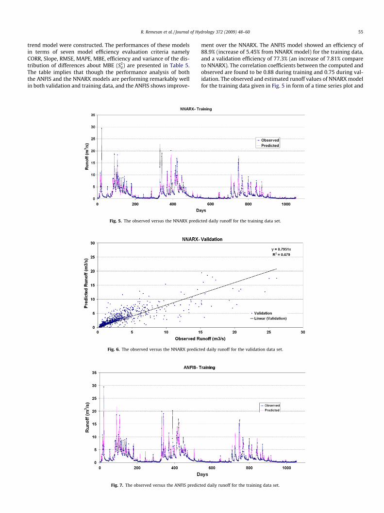
ment over the NNARX. The ANFIS model showed an efficiency of88.9% (increase of 5.45% from NNARX model) for the training data,and a validation efficiency of 77.3% (an increase of 7.81% compareto NNARX). The correlation coefficients between the computed andobserved are found to be 0.88 during training and 0.75 during val-idation. The observed and estimated runoff values of NNARX modelfor the training data given in Fig. 5 in form of a time series plot and

ted daily runoff for the training data set.

ed daily runoff for the validation data set.

ted daily runoff for the training data set.


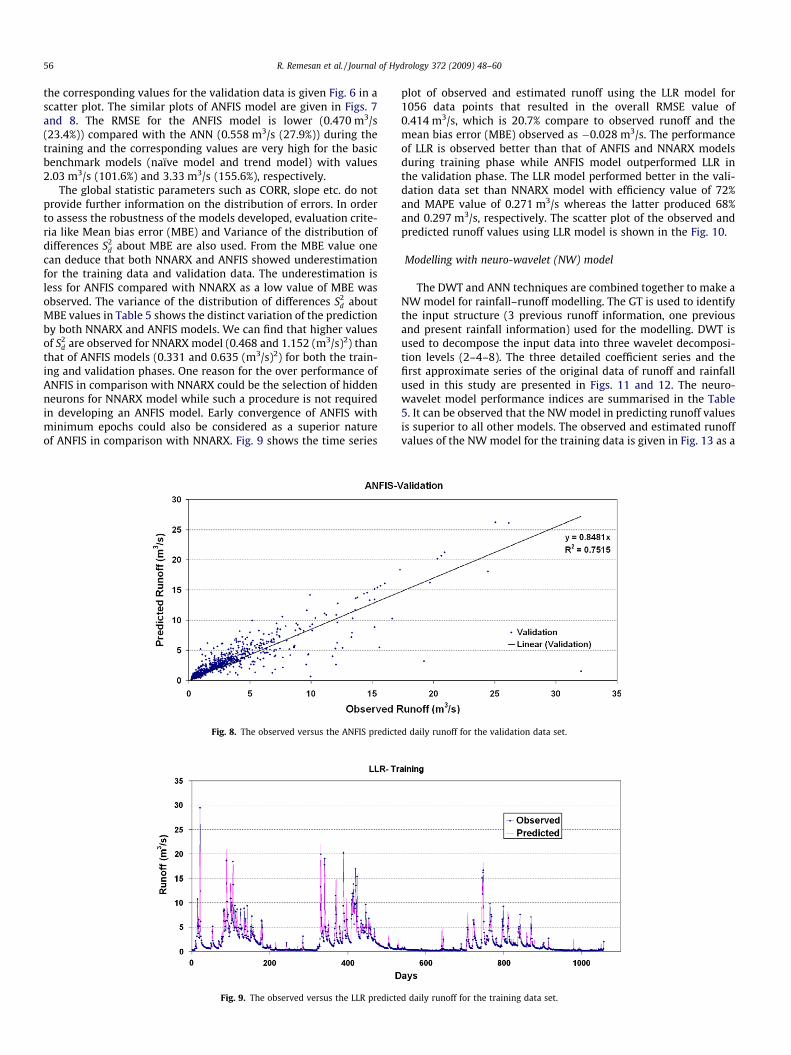
the corresponding values for the validation data is given Fig. 6 in ascatter plot. The similar plots of ANFIS model are given in Figs. 7and 8. The RMSE for the ANFIS model is lower (0.470 m3/s(23.4%)) compared with the ANN (0.558 m3/s (27.9%)) during thetraining and the corresponding values are very high for the basicbenchmark models (naïve model and trend model) with values2.03 m3/s (101.6%) and 3.33 m3/s (155.6%), respectively.

The global statistic parameters such as CORR, slope etc. do notprovide further information on the distribution of errors. In orderto assess the robustness of the models developed, evaluation crite-ria like Mean bias error (MBE) and Variance of the distribution ofdifferences S2

d about MBE are also used. From the MBE value onecan deduce that both NNARX and ANFIS showed underestimationfor the training data and validation data. The underestimation isless for ANFIS compared with NNARX as a low value of MBE wasobserved. The variance of the distribution of differences S2

d aboutMBE values in Table 5 shows the distinct variation of the predictionby both NNARX and ANFIS models. We can find that higher valuesof S2

d are observed for NNARX model (0.468 and 1.152 (m3/s)2) thanthat of ANFIS models (0.331 and 0.635 (m3/s)2) for both the train-ing and validation phases. One reason for the over performance ofANFIS in comparison with NNARX could be the selection of hiddenneurons for NNARX model while such a procedure is not requiredin developing an ANFIS model. Early convergence of ANFIS withminimum epochs could also be considered as a superior natureof ANFIS in comparison with NNARX. Fig. 9 shows the time series

Fig. 8. The observed versus the ANFIS predicte

Fig. 9. The observed versus the LLR predicte

plot of observed and estimated runoff using the LLR model for1056 data points that resulted in the overall RMSE value of0.414 m3/s, which is 20.7% compare to observed runoff and themean bias error (MBE) observed as �0.028 m3/s. The performanceof LLR is observed better than that of ANFIS and NNARX modelsduring training phase while ANFIS model outperformed LLR inthe validation phase. The LLR model performed better in the vali-dation data set than NNARX model with efficiency value of 72%and MAPE value of 0.271 m3/s whereas the latter produced 68%and 0.297 m3/s, respectively. The scatter plot of the observed andpredicted runoff values using LLR model is shown in the Fig. 10.

Modelling with neuro-wavelet (NW) model

The DWT and ANN techniques are combined together to make aNW model for rainfall–runoff modelling. The GT is used to identifythe input structure (3 previous runoff information, one previousand present rainfall information) used for the modelling. DWT isused to decompose the input data into three wavelet decomposi-tion levels (2–4–8). The three detailed coefficient series and thefirst approximate series of the original data of runoff and rainfallused in this study are presented in Figs. 11 and 12. The neuro-wavelet model performance indices are summarised in the Table5. It can be observed that the NW model in predicting runoff valuesis superior to all other models. The observed and estimated runoffvalues of the NW model for the training data is given in Fig. 13 as a

d daily runoff for the validation data set.

d daily runoff for the training data set.

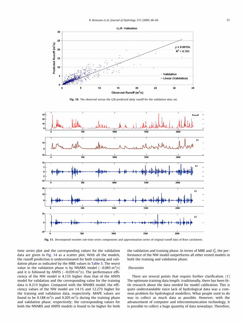
Fig. 10. The observed versus the LLR predicted daily runoff for the validation data set.

Fig. 11. Decomposed wavelet sub-time series components and approximation series of original runoff data of Brue catchment.


time series plot and the corresponding values for the validationdata are given in Fig. 14 as a scatter plot. With all the models,the runoff prediction is underestimated for both training and vali-dation phase as indicated by the MBE values in Table 5. The worstvalue in the validation phase is by NNARX model (�0.085 m3/s)and it is followed by ANFIS (�0.039 m3/s). The performance effi-ciency of the NW model is 4.13% higher than that of the ANFISmodel for validation and the corresponding value for the trainingdata is 8.21% higher. Compared with the NNARX model, the effi-ciency values of the NW model are 14.1% and 12.27% higher forthe training and validation data, respectively. MAPE values arefound to be 0.188 m3/s and 0.205 m3/s during the training phaseand validation phase, respectively; the corresponding values forboth the NNARX and ANFIS models is found to be higher for both

the validation and training phase. In terms of MBE and S2d , the per-

formance of the NW model outperforms all other tested models inboth the training and validation phase.

Discussion

There are several points that require further clarification. (1)The optimum training data length: traditionally, there has been lit-tle research about the data needed for model calibration. This isquite understandable since lack of hydrological data was a com-mon problem for hydrological modellers. What people used to dowas to collect as much data as possible. However, with theadvancement of computer and telecommunication technology, itis possible to collect a huge quantity of data nowadays. Therefore,

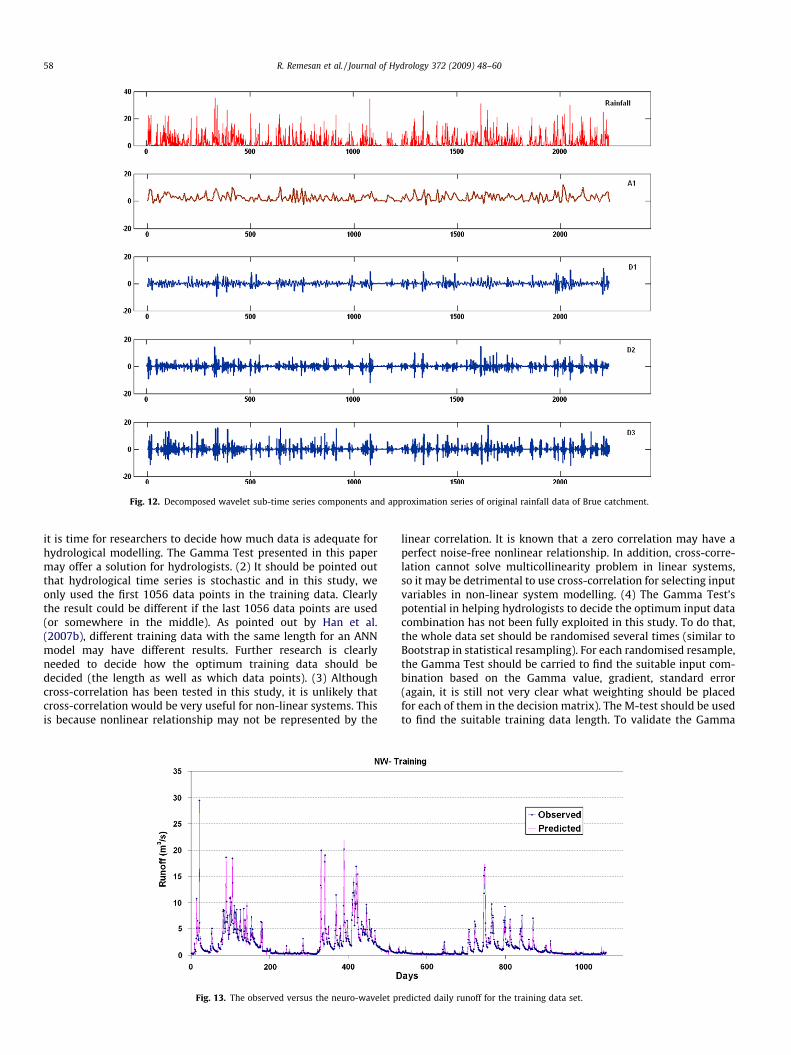
Fig. 12. Decomposed wavelet sub-time series components and approximation series of original rainfall data of Brue catchment.


it is time for researchers to decide how much data is adequate forhydrological modelling. The Gamma Test presented in this papermay offer a solution for hydrologists. (2) It should be pointed outthat hydrological time series is stochastic and in this study, weonly used the first 1056 data points in the training data. Clearlythe result could be different if the last 1056 data points are used(or somewhere in the middle). As pointed out by Han et al.(2007b), different training data with the same length for an ANNmodel may have different results. Further research is clearlyneeded to decide how the optimum training data should bedecided (the length as well as which data points). (3) Althoughcross-correlation has been tested in this study, it is unlikely thatcross-correlation would be very useful for non-linear systems. Thisis because nonlinear relationship may not be represented by the

Fig. 13. The observed versus the neuro-wavelet p

linear correlation. It is known that a zero correlation may have aperfect noise-free nonlinear relationship. In addition, cross-corre-lation cannot solve multicollinearity problem in linear systems,so it may be detrimental to use cross-correlation for selecting inputvariables in non-linear system modelling. (4) The Gamma Test’spotential in helping hydrologists to decide the optimum input datacombination has not been fully exploited in this study. To do that,the whole data set should be randomised several times (similar toBootstrap in statistical resampling). For each randomised resample,the Gamma Test should be carried to find the suitable input com-bination based on the Gamma value, gradient, standard error(again, it is still not very clear what weighting should be placedfor each of them in the decision matrix). The M-test should be usedto find the suitable training data length. To validate the Gamma

redicted daily runoff for the training data set.

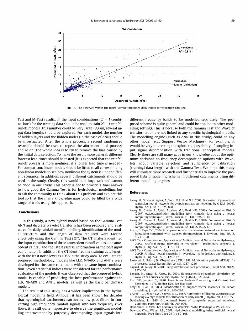
Fig. 14. The observed versus the neuro-wavelet predicted daily runoff for validation data set.


Test and M-Test results, all the input combinations (2n� 1 combi-nations) for the training data should be used to train 2n� 1 rainfallrunoff models (this number could be very large). Again, several in-put data lengths should be explored. For each model, the numberof hidden layers and the hidden nodes (in the case of ANN) shouldbe investigated. After the whole process, a second randomisedresample should be used to repeat the aforementioned process,and so on. The whole idea is to try to remove the bias caused bythe initial data selection. To make the result more general, differentforecast lead times should be tested (it is expected that the rainfallrunoff process is more nonlinear if a longer lead time is needed).For comparison, linear models should be fitted to all correspondingnon-linear models to see how nonlinear the system is under differ-ent scenarios. In addition, several different catchments should beused in the study. Clearly, this would be a huge task and cannotbe done in one study. This paper is not to provide a final answerto how good the Gamma Test is for hydrological modelling, butto ask the community to think about this problem and explore thistool so that the many knowledge gaps could be filled by a widerange of trials using this approach.

Conclusions

In this study, a new hybrid model based on the Gamma Test,ANN and discrete wavelet transform has been proposed and eval-uated for daily rainfall runoff modelling. Identification of the mod-el structure and the length of data required were tackledeffectively using the Gamma Test (GT). The GT analysis identifiedthe input combination of three antecedent runoff values, one ante-cedent rainfall and the latest rainfall information as the best inputcombination. In addition, the GT identified the training data lengthwith the least noise level as 1056 in the study area. To evaluate theproposed methodology, models like LLR, NNARX and ANFIS weredeveloped for the same catchment with the same input combina-tion. Seven statistical indices were considered for the performanceevaluation of the models. It was observed that the proposed hybridmodel is capable of producing the best performance against theLLR, NNARX and ANFIS models, as well as the basic benchmarkmodels.

The result of this study has a wider implication in the hydro-logical modelling field. Although it has been known for decadesthat hydrological catchments can act as low-pass filters in con-verting high frequency rainfall signals into low frequency riverflows, it is still quite impressive to observe the significant model-ling improvement by purposely decomposing input signals into

different frequency bands to be modelled separately. The pro-posed scheme is quite general and could be applied to other mod-elling settings. This is because both the Gamma Test and Wavelettransformation are not linked to any specific hydrological models.The modelling engine (such as ANN in this study) could be anyother model (e.g., Support Vector Machines). For example, itwould be very interesting to explore the possibility of coupling in-put signal decomposition with traditional conceptual models.Clearly there are still many gaps in our knowledge about the opti-mum decisions on frequency decomposition options with wave-lets, input variable selection and sufficiency of calibration(training) data length with the Gamma Test. We hope this studywill stimulate more research and further trials to improve the pro-posed hybrid modelling scheme in different catchments using dif-ferent modelling engines.

References

Aksoy, H., Guven, A., Aytek, A., Yuce, M.I., Unal, N.E., 2007. Discussion of generalizedregression neural networks for evapotranspiration modelling by O Kis�i (2006).Hydrol. Sci. J. 52 (4), 825–828.

Aksoy, H., Guven, A., Aytek, A., Yuce, M.I., Unal, N.E., 2008a. Comment on Kisi, O(2007) evapotranspiration modelling from climatic data using a neuralcomputing technique. Hydrol. Process. 21 (14), 1925–1934.

Aksoy, H., Guven, A., Aytek, A., Yuce, M.I., Unal, N.E., 2008b. Comment on Kisi, O(2007) evapotranspiration modelling from climatic data using a neuralcomputing technique. Hydrol. Process. 22 (14), 2715–2717.

Anctil, F., Tape, T.G., 2004. An exploration of artificial neural network rainfall–runoffforecasting combined with wavelet decomposition. J. Environ., Eng. Sci. 3,S121–S128.

ASCE Task Committee on Application of Artificial Neural Networks in Hydrology,2000a. Artificial neural networks in hydrology—I: preliminary concepts. J.Hydraul. Eng. ASCE 5 (2), 115–123.

ASCE Task Committee on Application of Artificial Neural Networks in Hydrology,2000b. Artificial neural networks in hydrology—II: hydrologic applications. J.Hydraul. Eng. ASCE 5 (2), 124–137.

Bartolini, P., Salas, J.D., Obeysekera, J.T.B., 1988. Multivariate periodic ARMA(1, 1)processes. Water Resour. Res. 24 (8), 1237–1246.

Bayazit, M., Aksoy, H., 2001. Using wavelets for data generation. J. Appl. Stat. 28 (2),157–166.

Bayazit, M., Onoz, B., Aksoy, H., 2001. Nonparametric streamflow simulation bywavelet or Fourier analysis. Hydrol. Sci. J. 46 (4), 623–634.

Box, G.E., Jenkins, G., 1970. Time Series Analysis Forecasting and Control, 2ndRevised ed. 1976. Holden-Day, San Francisco.

Bray, M., Han, D., 2004. Identification of support vector machines for runoffmodelling. J. Hydroinf. 6 (4), 265–280.

Chang, T.J., Delleur, J.W., Kavvas, M.L., 1987. Application of discrete autoregressivemoving average models for estimation of daily runoff. J. Hydrol. 91, 119–135.

Daubechies, I., 1988. Orthonormal bases of compactly supported wavelets.Commun. Pure Appl. Math. 41, 909–996.

Daubechies, I., 1992. Ten Lectures on Wavelets. SIAM, Philadelphia, PA. ch. 3-5.Dawson, C.W., Wilby, R.L., 2001. Hydrological modelling using artificial neural

networks. Prog Phys Geog 25 (1), 80–108.


Durrant, P.J., 2001. winGamma: A non-linear data analysis and modelling tool withapplications to flood prediction. Ph.D. Thesis, Department of Computer Science,Cardiff University, Wales, UK.

Evans, D., 2002. Data derived estimates of noise using near neighbour asymptotics.Ph.D. Thesis, Department of Computer Science, Cardiff University, Wales, UK.

Evans, D., Jones, A.J., 2002. A proof of the gamma test. Process. R. Soc. A 458 (2027),2759–2799.

Gautam, D., 2000. Neural network based system identification approach for themodelling of water resources and environmental systems. In: 2nd JointWorkshop on AI Methods in Civil Engineering ApplicationsCottbus/Germany,March 26–28, (http://www.bauinf.tu-cottbus.de/Events/Neural00/Participants.html).

Han, D., Cluckie, I.D., Karbassioun, D., Lawry, J., Krauskopf, B., 2002. River flowmodelling using fuzzy decision trees. Water Resour Manage 16 (6). December.

Han, D., Chan, L., Zhu, N., 2007a. Flood forecasting using support vector machines. J.Hydroinf. 9 (4), 267–276.

Han, D., Kwong, T., Li, S., 2007b. Uncertainties in real-time flood forecasting withneural networks. Hydrol. Process 21, 223–228.

Hecht-Nielsen, R., 1990. Neurocomputing. Addison-Wesley, Reading, MA.Horikawa, S., Furuhashi, T., Uchikawa, Y., 1992. On fuzzy modeling using fuzzy

networks woth back-propagation algorithm. IEEE Trans. Neural Networks 3 (5),801–806.

Jain, A., Sudheer, K.P., Srinivasulu, S., 2004. Identification of physical processesinherent in artificial neural network rainfall runoff models. Hydrol. Process. 18,571–581.

Jang, J.S.R., 1993. ANFIS: adaptive-network-based fuzzy inference system. IEEETrans. Syst. Manage. Cybern. 23 (3), 665–685.

Jonsdottir, H., Aa Nielsen, H., Madsen, H., Eliasson, J., Palsson, O.P., Nielsen, M.K.,2007. Conditional parametric models for storm sewer runoff. Water Res. Res.43, 1–9.

Karamouz, M., Razavi, S., Araghinejad, S., 2008. Long-lead seasonal rainfallforecasting using time-delay recurrent neural networks: a case study. Hydrol.Process. 22, 229–241.

Keller, J., Krishnapuram, R., Rhee, F.C.H., 1992. Evidence aggregation networks forfuzzy logic interface. IEEE Trans. Neural Network 3 (5), 761–769.

Kishor, N., Singh, S.P., 2007. Nonlinear predictive control for a NNARX hydro plantmodel. Neural Comput. Appl. 16 (2), 101–108.

Kisi, O., 2008. Stream flow forecasting using neuro-wavelet technique. Hydrol.Process. 22, 4142–4152.

Kosko, B., 1992 Fuzzy systems as universal approximators. In: Proc., IEEE Int. Conf.Fuzzy Syst, pp. 1153–1162.

Koutsoyiannis, D., 2007. Discussion of ‘‘generalized regression neural networks forevapotranspiration modelling” by O Kis�i (2006). Hydrol. Sci. J. 52 (4), 832–835.

Lafreni‘ere, M., Sharp, M., 2003. Wavelet analysis of inter-annual variability in therunoff regimes of glacial and nival stream catchments, Bow Lake, Alberta.Hydrol. Process. 17, 1093–1118.

Lane, S.N., 2007. Assessment of rainfall–runoff models based upon wavelet analysis.Hydrol. Process. 21, 586–607.

Maren, A.J., Harston, C.T., Pap, R.M., 1990. Handbook of Neural ComputingApplications. Academic Press, San Diego, CA.

Mechaqrane, A., Zouak, M., 2004. A comparison of linear and neural network ARXmodels applied to a prediction of the indoor temperature of a building. NeuralComput. Appl. 13, 32–37.

Morlet, J.M., Grossman, A., 1984. Decomposition of hardy functions into squareintegrable wavelets of constant shape. SIAM J. Math. Anal. 15 (4), 723–736.

Moss, M.E., Bryson, M.C., 1974. Autocorrelation structure of monthly streamflows.Water Resour. Res. 10 (4), 737–744.

Nayak, P.C., Sudheer, K.P., Rangan, D.M., Ramasastri, K.S., 2004. A neuro-fuzzycomputing technique for modelling hydrological time series. J. Hydrol. 291, 52–66.

Nayak, P.C., Sudheer, K.P., Rangan, D.M., Ramasastri, K.S., 2005. Short-term floodforecasting with a neurofuzzy model. Water Res. Res. 41, 1–16.

Nayak, P.C., Sudheer, K.P., Jain, S.K., 2007. Rainfall–runoff modeling through hybridintelligent system. Water Res. Res. 43, 1–17.

Partal, T., Kisi, O., 2007. Wavelet and neuro-fuzzy conjunction model forprecipitation forecasting. J. Hydrol. 342, 199–212.

Remesan, R., Shamim, M.A., Han, D., 2008. Model data selection using gamma testfor daily solar radiation estimation. Hydrol. Process. 22, 4301–4309.

See, L., Openshaw, S., 2000. Applying soft computing approaches to river levelforecasting. Hydrol. Sci. J. 44 (5), 763–779.

Sherman, L.K., 1932. Streamflow from rainfall by unit graph method. Eng. News-Rec. 108, 501–505.

Stefánsson, A., Koncar, N., Jones, A.J., 1997. A note on the gamma test. NeuralComput. Appl. 5 (3), 131–133.

Tao, P.C., Delleur, J.W., 1976. Seasonal and nonseasonal ARMA models in hydrology.J. Hydraul. Eng. ASCE 102 (HY10), 1541–1559.

Tayfur, G., Guldal, V., 2006. Artificial neural networks for estimating daily totalsuspended sediment in natural streams. Nord. Hydrol. 37 (1), 69–79.

Todini, E., 1978. Using a desk-top computer for an on-line flood warning system.IBM J. Res. Dev. 22, 464–471.

Unal, N.E., Aksoy, H., Akar, T., 2004. Annual and monthly rainfall data generationschemes. Stoch. Environ. Res. Risk Assess. 18 (4), 245–257.

Wang, W., Ding, J., 2003. Wavelet network model and its application to theprediction of the hydrology. Nature Sci 1 (1), 67–71.

Xingang, D., Ping, W., Jifan, C., 2003. Multiscale characteristics of the rainy seasonrainfall and interdecadal decaying of summer monsoon in North China. ChineseSci. Bull. 48, 2730–2734.

Xiong, L.H., Shamseldin, A.Y., O’Connor, K.M., 2001. A nonlinear combination of theforecasts of rainfall–runoff models by the first order Takagi-Sugeno fuzzysystem. J. Hydrol. 245 (1–4), 196–217.

Young, P.C., 2002. Advances in real-time flood forecasting. Philos. Trans. R. Soc. A360 (1796), 1433–1450.

Young, P.C., Garnier, H., 2006. Identification and estimation of continuous-time,data-based mechanistic (DBM) models for environmental systems. Environ.Modell. Software 21 (8), : 1055–1072.

Yueqing, X., Shuangcheng, L., Yunlong, C., 2004. Wavelet analysis of rainfallvariation in the Hebei Plain. Sci. China Ser. D. 48, 2241–2250.

Zadeh, L.A., 1965. Fuzzy sets. Inform. Control. 8 (3), 338–353.Zhou, H., Wu, L., Guo, Y., 2006. Mid and long term hydrologic forecasting for

drainage are based on WNN and FRM. In: Sixth international conference onintelligent systems design and applications, ISDA, 7–12.

http://www.bauinf.tu-cottbus.de/Events/Neural00/Participants.html

http://www.bauinf.tu-cottbus.de/Events/Neural00/Participants.html

runoff prediction using an integrated hybrid modelling scheme

Documents