rules + strategies for transforming lazy functional logic programs
TRANSCRIPT

Theoretical Computer Science 311 (2004) 479–525www.elsevier.com/locate/tcs
Rules + strategies for transforming lazyfunctional logic programs�;��
Mar()a Alpuentea , Moreno Falaschib , Gin(es Morenoc;∗ , Germ(an VidalaaDSIC, UPV, Camino de Vera s/n, 46022 Valencia, Spain
bDip. Mat. e Informatica, U. Udine, 33100 Udine, ItalycDep. Inform!atica, UCLM, 02071 Albacete, Spain
Received 2 October 2002; received in revised form 14 October 2003; accepted 14 October 2003
Abstract
This work introduces a transformation methodology for functional logic programs based onneeded narrowing, the optimal and complete operational principle for modern declarative lan-guages which integrate the best features of functional and logic programming. We provide cor-rectness results for the transformation system w.r.t. the set of computed values and answersubstitutions and show that the prominent properties of needed narrowing—namely, the opti-mality w.r.t. the length of derivations and the number of computed solutions—carry over to thetransformation process and the transformed programs. We illustrate the power of the system bytaking on in our setting two well-known transformation strategies (composition and tupling).We also provide an implementation of the transformation system which, by means of someexperimental results, highlights the potentiality of our approach.c© 2003 Elsevier B.V. All rights reserved.
Keywords: Program transformation; Functional logic programming; Strategies
1. Introduction
Functional logic programming languages combine the operational principles of themost important declarative programming paradigms, namely functional and logic
� This work has been partially supported by CICYT under grant TIC 98-0445-C03.�� A preliminary version of this article appeared in the Proceedings of the Fourth International Symposiumon Functional and Logic Programming, FLOPS’99 [4].
∗ Corresponding author.E-mail addresses: [email protected] (M. Alpuente), [email protected] (M. Falaschi),
[email protected] (G. Moreno), [email protected] (G. Vidal).
0304-3975/$ - see front matter c© 2003 Elsevier B.V. All rights reserved.doi:10.1016/j.tcs.2003.10.033
480 M. Alpuente et al. / Theoretical Computer Science 311 (2004) 479–525
programming (see [24] for a survey). EGcient demand-driven functional computationsare amalgamated with the Hexible use of logical variables providing for function inver-sion and search for solutions. The operational semantics of integratedlanguages is usually based on narrowing, a combination of variable instantiation andreduction. The instantiation of variables is often computed by unifying a subterm of thegoal expression with the left-hand side of some program rule; then narrowing reducesthe instantiated goal using that rule. Needed narrowing is currently the best narrowingstrategy for Jrst-order, lazy functional logic programs due to its optimality properties[9]. Needed narrowing provides completeness in the sense of logic programming (com-putation of all solutions) as well as functional programming (computation of values),and it can be eGciently implemented by pattern matching and uniJcation.
The fold=unfold transformation approach (also known as “rules+strategies” approach[41]) was Jrst introduced in [14] to optimize functional programs and then used forlogic programs [46]. This approach is based on the construction, by means of a strat-egy, of a sequence of equivalent programs—called transformation sequence and usu-ally denoted by R0; : : : ;Rn—where each program Ri is obtained from the preced-ing ones R0; : : : ;Ri−1 by using an elementary transformation rule. The essential rulesare folding and unfolding, i.e., contraction and expansion of subexpressions of a pro-gram using the deJnitions of this program (or of a preceding one). Other rules whichhave been considered are, e.g., instantiation, deJnition introduction=elimination, andabstraction.
There exists a large class of program optimizations which can be achieved byfold=unfold transformations and are not always possible by using a fully automaticmethod (such as partial evaluation [30]). Typical instances of this class are the strate-gies that perform tupling (also known as pairing) [14,20], which merges separate(non-nested) function calls with some common arguments into a single call to a (pos-sibly new) recursive function which returns a tuple of the results of the separate calls.Tupling is able to avoid either multiple accesses to the same data structures or com-mon subcomputations, similarly to the idea of sharing which is used in graph rewritingto improve the eGciency of computations in time and space [10]. A closely relatedstrategy is composition [48] (also known as fusion, deforestation, or vertical jamming[22]), which essentially consists of the merging of nested function calls, where theinner function call builds up a composite object which is used by the outer call; com-posing these two calls into one has the eNect to avoid the generation of the intermediatedata structure. Composition can be made automatically [48], whereas tupling has onlybeen automated to some extent (i.e., for particular classes of programs [15,16]) in the“rule+strategies” framework.
Although a lot of literature has been devoted to proving the correctness of fold=unfoldsystems w.r.t. the various semantics proposed for logic programs [12,23,31,36,40,46],in functional programming the problem of correctness has received surprisingly littleattention [42,43]. Of the very few studies of correctness of fold=unfold transformationsin functional programming, the most general and recent work is [42], which containscorrectness proofs for several well-known transformation methods (like Wadler’s de-forestation [48]).

M. Alpuente et al. / Theoretical Computer Science 311 (2004) 479–525 481
In [3], we investigated fold=unfold rules in the context of a strict (call-by-value)functional logic language based on unrestricted (i.e., not optimized) narrowing. Theuse of narrowing empowers the fold=unfold system by implicitly embedding the in-stantiation rule (the operation of the Burstall and Darlington framework [14] whichintroduces an instance of an existing equation) into unfolding by means of uniJcation.However, [3] does not consider a general transformation system (only two rules: foldand unfold), and hence the composition or tupling transformations cannot be achieved.Also, [3] refers to a notion of “reversible” folding, whose optimization power within atransformation system is very poor. On the other hand, the use of unrestricted narrow-ing to perform unfolding may produce an important increase in the number of programrules.
In this work, we deJne a transformation methodology for lazy (call-by-name) func-tional logic programs. On the theoretical side, we extend the Tamaki and Sato trans-formation rules [46] for logic programs to cope with lazy functional logic programsbased on needed narrowing. The transformation process consists of applying an arbi-trary number of times the basic transformation rules, which are: deJnition introduction,deJnition elimination, unfolding, folding, and abstraction. Needed narrowing is com-plete for inductively sequential programs [7]. Thus, we demonstrate that such a programstructure is preserved through a transformation sequence (R0; : : : ;Rn), which is a keypoint for proving the correctness of the transformation system as well as for its eNectiveapplicability. For instance, by using other variants of narrowing (e.g., lazy narrowing[39]), the structure of the original program is not preserved, thus seriously restrictingthe applicability of the transformation system: the transformed program could not befurther transformed and, what is even worse, it might not even be safely executed,as it might not satisfy the conditions for the completeness of the considered opera-tional mechanism. The major technical result consists of proving strong correctness forthe transformation system, namely that the values and answers computed by needednarrowing in the initial and the Jnal program coincide (for goals constructed usingthe symbols of the initial program). The eGciency improvement of Rn with regardto R0 is not ensured by an arbitrary use of the elementary transformation rules butit rather depends on the heuristic which is employed. Hence, on the practical side,we investigate how the classical and powerful transformation methodologies of tuplingand composition [41] transfer to our framework. We show the advantages of usingneeded narrowing in this framework, and illustrate the power of our transformationsystem by (automatically) optimizing several signiJcant examples using a prototypeimplementation [2].
The structure of the paper is as follows. After recalling some basic deJnitions inthe next section, we introduce the basic transformation rules and illustrate them bymeans of several examples in Section 3. We state the correctness of the transformationsystem and show some results about the structure of transformed programs in Section 4.Section 5 shows how to achieve the (automatic) composition and tupling strategies inour framework, whereas Section 6 presents an experimental evaluation of the method ona set of benchmarks. Finally, Section 7 concludes. We include an appendix containingthe proofs of some technical results.

482 M. Alpuente et al. / Theoretical Computer Science 311 (2004) 479–525
2. Preliminaries
We assume familiarity with basic notions of term rewriting [10] and functional logicprogramming [24]. We consider a signature � partitioned into a set C of constructorsand a set F of (deJned) functions or operations. We write c=n∈C and f=n∈Ffor n-ary constructor and operation symbols, respectively. There is at least one sortBool containing the 0-ary Boolean constructors true and false. The set of terms andconstructor terms with variables (e.g., x; y; z) from X are denoted by T(C∪F;X)and T(C;X), respectively. The set of variables occurring in a term t is denoted byVar(t). A term is linear if it does not contain multiple occurrences of any variable.We write on for the list of syntactic objects o1; : : : ; on.
A pattern is a term of the form f(dn) where f=n∈F and d1; : : : ; dn ∈T(C;X).Note the diNerence with the usual notion of pattern in functional programming: aconstructor term. A term is operation-rooted (constructor-rooted) if it has an oper-ation (constructor) symbol at the root. A position p in a term t is represented bya sequence of natural numbers (� denotes the empty sequence, i.e., the root posi-tion). Positions are ordered by the pre7x ordering: p6q, if ∃w such that p:w= q.Positions p; q are disjoint if neither p6q nor q6p. Given a term t, we let Pos(t)and NVPos(t) denote the set of positions and the set of non-variable positions of t(i.e., positions where a variable does not occur), respectively. t|p denotes the subtermof t at position p, and t[s]p denotes the result of replacing the subterm t|p by theterm s.
We denote by {x1 �→ t1; : : : ; xn �→ tn} the substitution � with �(xi) = ti for i= 1; : : : ; n(with xi = xj if i = j), and �(x) = x for all other variables x. A substitution � is (ground)constructor, if �(x) is (ground) constructor for all x such that �(x) = x. The identitysubstitution is denoted by id. Given a substitution � and a set of variables V ⊆X,we denote by ��V the substitution obtained from � by restricting its domain to V . Wewrite �= �[V ] if ��V = ��V , and �6�[V ] denotes the existence of a substitution � suchthat � ◦ �= � [V ]. We write t6t′ (subsumption) if t′ = �(t) for some substitution �;moreover, we write t¡t′ (strict subsumption) if � = id. A uni7er of two terms s andt is a substitution � with �(s) = �(t). A uniJer � of s and t is most general (mgu)if �6� for each uniJer � of s and t (such a mgu is unique up to renaming). Twosubstitutions � and �′ are disjoint (on a set of variables V ) if there exists some x∈Vsuch that �(x) and �′(x) are not uniJable.
A set of rewrite rules l→ r such that l =∈X, and Var(r)⊆Var(l) is called a termrewriting system (TRS). Terms l and r are called the left-hand side (lhs) and theright-hand side (rhs) of the rule, respectively. A TRS R is left-linear if l is linearfor all l→ r ∈R. A TRS is constructor based (CB) if each lhs is a pattern. In theremainder of this paper, a functional logic program is a left-linear CB-TRS. Conditionsin program rules are treated by using the predeJned functions and, if then else,case of which are reduced by standard deJning rules [25,39]. Two (possibly renamed)rules l→ r and l′ → r′ overlap if there is a non-variable position p∈NVPos(l) anda substitution � such that �(l|p) = �(l′). A left-linear TRS with no overlapping rulesis called orthogonal. A rewrite step is an application of a rewrite rule to a term, i.e.,t→p;R s if there exists a position p in t, a rewrite rule R= l→ r and a substitution �

M. Alpuente et al. / Theoretical Computer Science 311 (2004) 479–525 483
with t|p = �(l) and s= t[�(r)]p (p and R will often be omitted in the denotation of arewrite step). The instantiated lhs �(l) is called a redex. A term t is called a normalform if there is no term s with t→ s. →+ denotes the transitive closure of → and →∗
denotes the reHexive and transitive closure of →.In orthogonal TRSs, every term which is not a normal form has a needed redex that
must “eventually” be reduced to normalize the term [28,32]. Therefore, for orthogonalTRSs, the best normalizing strategy which avoids unnecessary reductions is neededrewriting [28], a reduction strategy which only considers needed redexes, namely, re-dexes which must be contracted (themselves or some descendant) in every derivationleading to a normal form. Unfortunately, it is undecidable whether a redex is neededand can only be approximated. For CB-TRSs, Antoy’s outermost-needed redexes [7]provide a decidable subclass of needed redexes which can be used to normalize termsin a particular class of programs, called inductively sequential systems, by applyingoutermost-needed reduction. The formal deJnition of outermost-needed rewriting canbe found in [8,9], and will be recalled in Appendix B.
In order to evaluate terms containing variables, the narrowing mechanism non-deterministically instantiates the variables so that a rewrite step is possible. Formally,t❀p;R; � t′ is a narrowing step if p is a non-variable position in t and �(t)→p;R t′. Wedenote by t0 ❀∗
� tn a sequence of narrowing steps t0 ❀�1 : : : ❀�n tn with �= �n ◦ · · · ◦�1 (where �= id for n= 0). Since we are interested in computing values (constructorterms) as well as answers (substitutions) in functional logic programming, we say thatthe narrowing derivation t❀∗
� c computes the result c with answer � if c is a construc-tor term. The evaluation to (ground) constructor terms (and not to arbitrary expressions)is the intended semantics of functional languages and also of most functional logic lan-guages. In particular, the equality predicate ≈ used in some examples is deJned, like infunctional languages, as the strict equality on terms, i.e., the equation t1 ≈ t2 is satisJedif t1 and t2 are reducible to the same ground constructor term. A solution of an equations≈ t is a substitution � such that �(s≈ t) can be reduced to true. On the other hand, wesay that � is a computed answer substitution for an equation e if there is a narrowingderivation e❀∗
� true.
2.1. Needed narrowing
A challenge in the design of functional logic languages is the deJnition of a “good”narrowing strategy, i.e., a restriction on the narrowing steps issuing from a term with-out losing completeness. Needed narrowing [9] is currently the best known narrowingstrategy due to its optimality properties w.r.t. the length of the derivations and the num-ber of computed solutions. It extends Huet and L(evy’s notion of a needed reduction[28]. The deJnition of needed narrowing [9] uses the notion of a de7nitional tree [7].DeJnitional trees are similar to standard matching trees of functional programming.However, diNerently from left-to-right matching trees used in either Hope, Miranda,or Haskell, deJnitional trees deal with dependencies between arguments of functionalpatterns. Roughly speaking, a deJnitional tree for a function symbol f is a tree whoseleaves contain all (and only) the rules used to deJne f and whose inner nodes containinformation to guide the (optimal) pattern matching during the evaluation of expres-

484 M. Alpuente et al. / Theoretical Computer Science 311 (2004) 479–525
sions. Each inner node contains a pattern and a variable position in this pattern (theinductive position) which is further reJned in the patterns of its immediate childrenby using diNerent constructor symbols. The pattern of the root node is simply f(xn),where xn are diNerent variables.
Formally, a de7nitional tree of a Jnite set of linear patterns S is a Jnite non-empty set P of linear patterns partially ordered by subsumption having the followingproperties (up to variable renaming):
Root property: There is a minimum element pattern(P), also called the pattern ofthe deJnitional tree.
Leaves property: The maximal elements, called the leaves, are the elements of S. Non-maximal elements are also called branches.
Parent property: If $∈P, $ =pattern(P), there exists a unique $′ ∈P, called theparent of $ (and $ is called a child of $′), such that $′¡$ and there is no otherpattern $′′ ∈T(C∪F;X) with $′¡$′′¡$.
Induction property: Given $∈P\S, there is a position o—the inductive position—ofpattern(P) with pattern(P)|o ∈X and constructors c1; : : : ; cn ∈C with ci = cj fori = j, such that, for all $1; : : : ; $n which have the parent $, $i = $[ci(xni)]o (wherexni are new distinct variables) for all 16i6n.
Given a deJned function f=n in a program R, we say that P is a de7nitionaltree of f if pattern(P) =f(xn) for distinct variables xn and the leaves of P areall and only variants of the left-hand sides of the rules in R deJning f. A de-Jned function is called inductively sequential if it has a deJnitional tree. A rewritesystem R is called inductively sequential if all its deJned functions are inductivelysequential. Observe that every inductively sequential TRS is orthogonal, but the in-verse does not generally hold. For instance, the following orthogonalTRS:
f(X; a; b) → a f(b; X; a) → b f(a; b; X) → c
where X is a variable and a; b; c are constructor symbols, is not inductively sequen-tial since there is no deJnitional tree for function f. An inductively sequential TRScan be viewed as a set of deJnitional trees, each one deJning a function symbol.There can be more than one deJnitional tree for an inductively sequential function.In the following, we assume that there is a Jxed deJnitional tree for each deJnedfunction.
It is often convenient and simpliJes the understanding to provide a graphic repre-sentation of deJnitional trees, where each node is marked with a pattern, the inductiveposition in branches is surrounded by a box, and the leaves contain the correspondingrules. For instance, the deJnitional tree for the function “6”:
0 6 N → true
s(M) 6 0 → false
s(M) 6 s(N) → M6 N

M. Alpuente et al. / Theoretical Computer Science 311 (2004) 479–525 485
can be depicted as follows:
For the deJnition of needed narrowing, we assume that t is an operation-rooted termand P is a deJnitional tree with pattern(P) = $ such that $6t. We deJne a function% from terms and deJnitional trees to sets of tuples (position, rule, substitution) as theleast set satisfying the following properties. We consider two cases for P:(1) If $ is a leaf, i.e., P= {$}, and $→ r is a variant of a rewrite rule, then
%(t;P) = {(�; $ → r; id)}:
(2) If $ is a branch, consider the inductive position o of $ and some child $i =$[ci(xn)]o ∈P. Let Pi = {$′ ∈P | $i6$′} be the deJnitional tree where all patternsare instances of $i. Then we consider the following cases for the subterm t|o:
%(t;P) �
(p; R; � ◦ &) if t|o = x∈X, & = {x �→ ci(xn)}, and(p; R; �)∈ %(&(t);Pi);
(p; R; � ◦ id) if t|o = ci(tn) and (p; R; �)∈ %(t;Pi);
(o:p; R; � ◦ id) if t|o = f(tn) for f∈F and(p; R; �)∈ %(t|o;P′) where P′
is a deJnitional tree for f.
Informally speaking, needed narrowing directly applies a rule if the term is an in-stance of some left-hand side (case 1), or checks the subterm corresponding to theinductive position of the branch (case 2): if it is a variable, it is instantiated to theconstructor of some child; if it is already a constructor, we proceed with the correspond-ing child; if it is a function, we evaluate it by recursively applying needed narrowing.Thus, the strategy diNers from lazy functional languages only in the instantiation offree variables. In contrast to more traditional narrowing strategies, needed narrowingdoes not compute most general uniJers. In each recursive step during the computa-tion of %, we compose the current substitution with the local substitution of this step(which can be the identity). Thus, each needed narrowing step can be represented as(p; R; ’k ◦ · · · ◦’1), where each binding ’j is either the identity or the replacement ofa single variable. This is called the canonical representation of a needed narrowingstep.
As in proof procedures for logic programming, we assume that deJnitional treesalways contain new variables if they are used in a narrowing step. This implies that

486 M. Alpuente et al. / Theoretical Computer Science 311 (2004) 479–525
all computed substitutions are idempotent (we will implicitly assume this property inthe following).
To compute needed narrowing steps for an operation-rooted term t, we take a deJ-nitional tree P for the root of t and compute %(t;P). Then, for all (p; R; �)∈ %(t;P),t❀p;R; � t′ is a needed narrowing step.
Example 1. Consider again the rules for “6” together with the following rules deJningthe addition on natural numbers:
0 + N → Ns(M) + N → (sM + N)
Then, the function % computes the following set for the initial term X6X + X:
{(�; 0 6 N → true; {X �→ 0}); (2,s(M) + N → (sM + N); {X �→ s(M)})}
This corresponds to the following narrowing steps (the subterm evaluated in the nextstep is underlined):
X6 X + X ❀{X �→0} trueX6 X + X ❀{X �→s(M)} s(M) 6 s(M + s(M))
Needed narrowing is sound and complete for inductively sequential programs. More-over, it is minimal, i.e., given two distinct needed narrowing derivations e❀∗
� true ande❀∗
�′ true, we have that � and �′ are disjoint on Var(e). These properties are formal-ized as follows:
Theorem 2 (Antoy et al. [9]). Let R be an inductively sequential program and e anequation.(1) (Soundness) If e❀∗
� true is a needed narrowing derivation, then � is a solutionfor e.
(2) (Completeness) For each constructor substitution � that is a solution of e, thereexists a needed narrowing derivation e❀∗
�′ true with �′6� [Var(e)].(3) (Minimality) If e❀∗
� true and e❀∗�′ true are two distinct needed narrowing deri-
vations, then � and �′ are disjoint on Var(e).
3. The transformation rules
In this section, our aim is to deJne a set of program transformations which is stronglycorrect, i.e., sound and complete w.r.t. the semantics of values and answer substitu-tions computed by needed narrowing. Let us Jrst give the rule for the introductionand elimination of function deJnitions in a similar style to [46], in which the set ofdeJnitions is partitioned into “old” and “new” functions. In the following, we considera Jxed transformation sequence (R0; : : : ;Rk), k¿0.

M. Alpuente et al. / Theoretical Computer Science 311 (2004) 479–525 487
De�nition 3 (DeJnition introduction). We may get program Rk+1 by adding to Rk anew rule (called a “deJnition rule” or “eureka”) of the form f(tn)→ r, such that:(1) f(tn) is a linear pattern and Var(f(tn)) = Var(r)—i.e., the rule is non-erasing—,(2) f does not occur in the sequence R0; : : : ;Rk (f is new), and(3) every deJned function symbol occurring in r belongs to R0.We say that f is a new function symbol, and every function symbol belonging to R0
is called an old function symbol.
The introduction of a new eureka deJnition is virtually always the Jrst step of atransformation sequence. Determining which deJnitions should be introduced is a clevertask (which justiJes the name “eureka” for the new rules) which falls into the realmof strategies (see [40] for a survey), as we discuss in Section 5. Let us note that onlyone program rule can be introduced with our deJnition introduction rule. This meansthat function deJnitions consisting of several rules with diNerent patterns in the left-hand side cannot be introduced. Nevertheless, this is not a limitation in practice sincethe rules introduced by the transformation strategies which we consider in Section 5have the form f(xn)→ exp, where xn are the diNerent variables occurring in exp. Thisis common in almost all transformation strategies that can be found in the literature.Now, we would like to advance two important aspects which are strongly related withthe folding operation that we will see later:(1) A eureka rule maintains its status only as long as no transformation step is applied
on it. Once we transform this rule—even if the resulting rule is syntactically equalto the original one—it is not considered a eureka rule anymore. As we will seein DeJnition 8, this is important for the folding operation, since we can only foldnon-eureka rules using eureka rules.
(2) The non-erasing condition is required for avoiding the creation of rules with extra-variables when performing folding steps. Consider, for instance, the folding of rulef(X)→ g(X) using the (incorrect) eureka new(X; Y)→ g(X) which would produce anew rule f(X)→ new(X; Y) containing an extra-variable in its rhs (thus an illegalrule).
De�nition 4 (DeJnition elimination). We may get program Rk+1 by deleting from pro-gram Rk all rules deJning the functions f0; : : : ; fn (n¿0), say Rf, such that f0; : : : ; fndo not occur in R0 nor in (Rk − Rf).
This rule has been initially proposed with the name of deletion (for logic programs)in [36] and also in [12], where it was called restriction. Note that the deletion of therules deJning a function f implies that no function calls to f are allowed afterwards.However, subsequent transformation steps (in particular, folding steps) might introducethose deleted functions in the rhs’s of the rules, thus producing inconsistencies in theresulting programs. We avoid this encumbrance by the usual requirement [40]: do notallow folding steps if a deJnition elimination has been previously performed.
Now we introduce our unfolding rule, which systematizes a Jt combination of in-stantiation and classical (functional) unfolding into a single transformation. Essentially,it exploits the capability of narrowing to deal with logical variables.

488 M. Alpuente et al. / Theoretical Computer Science 311 (2004) 479–525
De�nition 5 (Unfolding). Let R= (l→ r)∈Rk be a rule (the “unfolded rule”) whoserhs is an operation-rooted term. We may get program Rk+1 from Rk by replacing Rwith the set of rules:
{�(l) → r′ | r ❀� r′ is a needed narrowing step in Rk}:
Here, it is worth noting that the requirement not to unfold a rule whose rhs isconstructor-rooted can be left aside when functions are totally de7ned (which is quiteusual in typed languages). The following example shows that the above requirementcannot be dropped in general.
Example 6. Consider the following programs:
R =
f(0) → 0g(X) → s(f(X))
h(s(X)) → s(0)
R′ =
f(0) → 0g(0) → s(0)
h(s(X)) → s(0)
We get R′ from R by applying an unfolding step which considers the needed narrowingderivation s(f(X))❀{X �→0} s(0) for the rhs of the second rule in R. Now, the termh(g(s(0))) has the following needed narrowing derivation in R:
h(g(s(0))) ❀ h(s(f(s(0)))) ❀ s(0)
whereas it is no longer possible in the transformed program. Essentially, completenessis lost because the unfolding rule, f(0)→ 0, deJnes a function f which is not totallydeJned. Hence, by unfolding the call f(X) we improperly “compile in” an unnecessaryrestriction in the domain of the function g.
The following example illustrates the fact that the choice of the operational principleof needed narrowing to drive the unfolding steps is not only convenient but also crucialto guarantee that the structure of the original program, i.e., inductive sequentiality, ispreserved through the transformation.
Example 7. Consider the following inductively sequential (hence also orthogonal) pro-gram:
test(X; Y) → h(f(X; g(Y))) g(0) → g(0)
f(0; 0) → s(f(0; 0)) h(s(X)) → 0
f(s(N); X) → s(f(N; X))
Note that the goal test(X,Y) reduces to 0 if X is bound to s(N), and it enters a loopif X is bound to 0 due to the non-terminating evaluation of g(0).

M. Alpuente et al. / Theoretical Computer Science 311 (2004) 479–525 489
Now, by unfolding the Jrst rule using needed narrowing and lazy narrowing, 1 re-spectively, we obtain the following rules in the respective programs:
Rneeded ={
test(0; 0) → h(f(0; g(0)))test(s(X); Y) → h(s(f(X; g(Y))))
}
Rlazy ={
test(X; 0) → h(f(X; g(0)))test(s(X); Y) → h(s(f(X; g(Y))))
}
Note that Rlazy is neither inductively sequential nor orthogonal, in contrast to theoriginal program R. This does not only mean that the unfolded program cannot beexecuted by using needed narrowing (nor lazy narrowing), but also that Rlazy has aworse termination behaviour than Rneeded (and also worse than R). For instance, theterm test(s(0),0) has a Jnite derivation tree w.r.t. Rneeded (using either needed or lazynarrowing) whereas the (lazy narrowing) derivation tree w.r.t. Rlazy is inJnite in depth(caused by the application of the rules test(X; 0)→ h(f(X; g(0))) and g(0)→ g(0)).
Now, let us introduce the folding rule, which is a counterpart of the previous trans-formation, i.e., the compression of a piece of code into an equivalent call.
De�nition 8 (Folding). Let R= (l→ r)∈Rk be a rule (the “folded rule”) and letR′ = (l′ → r′)∈Rj, 06j6k, be a rule (the “folding rule”) such that r|p = �(r′) forsome position p∈NVPos(r) and substitution �, fulJlling the following conditions:(1) the folded rule R is not a eureka rule and(2) the folding rule R′ is a eureka rule.Then, we may get program Rk+1 from program Rk by replacing the rule R with thenew rule l→ r[�(l′)]p.
Roughly speaking, the folding operation proceeds in a contrary direction to the usualreduction steps, i.e., reductions are performed against the reversed folding rules. Thereare several points regarding our deJnition of the folding rule which are worth noticing:• The condition which says that the folded rule R is not a eureka rule means that
either l (the lhs of R) is rooted by an old function symbol or R is the result ofunfolding a eureka rule at least once within the sequence R0; : : : ;Rk .
• In contrast to the unfolding rule, the subterm which is selected for the folding stepneeds not be a (needed) narrowing redex. This generality is not only safe but alsohelpful as it will become apparent in Section 5.
• The substitution � of DeJnition 8 is not a uniJer (as occurs in the more in-volved version of [3]) but just a matcher, similarly to many other folding rulesfor logic programs, which have been deJned in a similar “functional style” (see,e.g., [12,31,41,46]). Moreover, it has the extra advantage that it is easier to checkand can still produce—at a very low cost—many powerful optimizations.
1 We consider the (demand-driven) lazy narrowing strategy described in [39], which is also driven by thepatterns in the lhs’s of the rules (though it is “less lazy” than needed narrowing).

490 M. Alpuente et al. / Theoretical Computer Science 311 (2004) 479–525
Many proposals have also been made to deJne a folding transformation in a (pure)functional context [14,18,33,43]. A marked folding for a lazy (higher-order) functionallanguage has been presented in [42], which preserves the semantics of (ground con-structor) values under applicability conditions which are similar to ours. However, ourcorrectness results are slightly stronger, since we preserve the (non-ground) semanticsof computed values and answers.
As in our deJnition of folding, a large number of proposals also allow the foldedand the folding rule to belong to diNerent programs (see, e.g., [12,31,40,41,46]), whichis crucial to achieve an eNective optimization in many cases. Some other works inthe literature have advocated a diNerent style of folding which is reversible [23], i.e.,a kind of folding which can always be undone by an unfolding step. This greatlysimpliJes the correctness proofs—correctness of folding follows immediately from thecorrectness of unfolding—, but usually require too strong applicability conditions, suchas requiring that both the folded and the folding rules belong to the same program. Thisdrastically reduces the power of the transformation. The folding rule proposed in [3]for a strict functional logic language is reversible and thus its transformational poweris very limited. Our folding rule is more powerful and practical since the applicabilityconditions are less restrictive. Therefore, its use within a transformation system—whenguided by appropriate strategies—is able to produce more eNective optimizations for(lazy) functional logic programs.
The set of rules presented so far constitutes the kernel of our transformation sys-tem. These rules suGce to automate the composition strategy (see Section 5). Other(functional) approaches include a new rule called abstraction [14,42] (often knownas where–abstraction rule [41]) that can be simulated in our setting by applying ap-propriate deJnition introduction and folding steps. This rule is usually required toimplement tupling and it essentially consists of replacing the occurrences of someexpression e in the rhs of a rule R by a fresh variable z, adding the“local declaration” z = e within a where expression in R. For instance, therule
double sum(X; Y) → sum(sum(X; Y); sum(X; Y))
can be transformed into the new rule
double sum(X,Y) → sum(Z; Z) where Z = sum(X; Y):
As noted by [41], the use of the where-abstraction rule has the advantage that, in thecall-by-value mode of execution, the evaluation of the expression e is performed onlyonce. This is also true in a lazy context under an implementation based on sharing,which allows us to keep track of variables which occur several times in the expressionto be evaluated.
The new rules introduced by the where-abstraction rule often contain extra variablesin the right-hand sides. However, as noted in [42], this can easily be amended byusing standard “lambda lifting” techniques (which can be thought of as an appropriateapplication of a deJnition introduction step followed by a folding step). For instance,

M. Alpuente et al. / Theoretical Computer Science 311 (2004) 479–525 491
if we consider again the rule
double sum(X; Y) → sum(Z; Z) where Z = sum(X; Y);
we can transform it (by lambda lifting [29]) into the new pair of rules:
double sum(X,Y) → ds aux(sum(X,Y))ds aux(Z) → sum(Z,Z)
Note that these rules can be directly generated from the initial deJnition by a deJni-tion introduction (ds aux(Z)→ sum(Z; Z)) and then by folding the original rule at theexpression sum(sum(X; Y); sum(X; Y)) using as folding rule the newly generated deJnitionfor ds aux. The inclusion of an abstraction rule is traditional in functional fold=unfoldframeworks [14,41–43]. In the case of logic programs, abstraction is only possible bymeans of the so called generalization strategy [41], which generalizes some calls toeliminate the mismatches that prevent a folding step.
Now, we are ready to formalize our abstraction rule, which is inspired by the standardlambda lifting transformation of functional programs. By means of the tuple constructor〈 〉, our deJnition allows the abstraction of diNerent expressions in one go. For asequence of (pairwise disjoint) positions P =pn, we let t[sn]P = (((t[s1]p1 )[s2]p2 ) : : :[sn]pn). By abuse, we denote t[sn]P by t[s]P when s1 = · · ·= sn = s, as well as ((t[s1]P1 ): : : [sn]Pn) by t[sn]Pn
.
De�nition 9 (Abstraction). Let R= (f(tn)→ r)∈Rk be a non-eureka rule and let Pjbe sequences of disjoint positions in NVPos(r) such that r|p = ei for all p in Pi,i= 1; : : : ; j, i.e., r = r[ej]Pj . We may get program Rk+1 from program Rk by replacingR with the rules:
Rabs = (f(tn) → f aux(ym; 〈e1; : : : ; ej〉))Rnew = (f aux(ym; 〈z1; : : : ; zj〉) → r[zj]Pj
)
where zj are fresh variables not occurring in tn, Var(r[zj]Pj) = {ym; zj}, f aux is a newfunction symbol that does not occur in (R0; : : : ;Rk), and, on the contrary, r[zj]Pj doesnot contain new function symbols.
As we mentioned before, the transformation which is achieved by our abstractionrule can also be obtained, in our framework, by a deJnition introduction step (thatgenerates the eureka rule Rnew) followed by a folding step (that folds the rule to beabstracted R using Rnew and delivers the desired rule Rabs). Informally speaking, thetwo rules generated by the abstraction transformation can be seen as a syntactic variantof the following rule:
f(tn) → r[zj]Pjwhere 〈z1; : : : ; zj〉 = 〈e1; : : : ; ej〉
using the conventional notation of where clauses. In the examples shown in Sections 5and 6, we will use this sugared syntax for readability reasons.

492 M. Alpuente et al. / Theoretical Computer Science 311 (2004) 479–525
4. Correctness properties of the transformation system
In this section, we state and prove the main theoretical results for the transforma-tion system based on the elementary rules introduced so far: deJnition introduction,deJnition elimination, unfolding, folding, and abstraction. We state the correctness ofthe transformation system, as well as the preservation of the structure of programs,for transformation sequences constructed from an inductively sequential program. Inproving this, we assume that no folding step is applied after a deJnition elimination,which guarantees that no function call to a previously deleted function is introduced[40]. The following example illustrates the need for this requirement.
Example 10. Consider the following inductively sequential program Ri:
f(X) → 0 (R1)g(X) → 0 (R2)
and assume that R2 is a eureka rule. Firstly, we perform a deJnition elimination stepon the new function g. In this way, we obtain program Ri+1:
f(X) → 0 (R1)
Now, we fold R1 ∈Ri+1 using the folding rule R2 ∈Ri, obtaining Ri+2:
f(X) → g(X) (R3)
Observe that the term f(X) can be reduced to 0 in Ri and Ri+1 but not in Ri+2. Theproblem arises because the folding rule (unlike any other transformation rule) is ableto introduce new symbols in the rhs of a rule, even when these function symbols areundeJned (since the rules deJning them have been previously removed).
Therefore, we only consider transformation sequences fulJlling the following condi-tions:• the initial program of the transformation sequence is inductively sequential, and• no folding step is applied after a deJnition elimination step.Moreover, since the abstraction rule can easily be recast in terms of deJnition intro-duction and folding, w.l.o.g., in the following we restrict ourselves to transformationsequences which do not use this rule.
The following theorem states that transformation sequences preserve the inductivelysequential structure of programs:
Theorem 11. Let (R0; : : : ;Rn), n ¿ 0, be a transformation sequence such that R0 isan inductively sequential program. Then, Ri is inductively sequential, for i= 1; : : : ; n.
The formal proof can be found in Appendix A. Essentially, this result is a directconsequence of the following facts:• By applying a deJnition introduction=elimination transformation to a given program,
we simple add=remove some deJnitional trees for new=old rules, and hence theresulting program is inductively sequential.

M. Alpuente et al. / Theoretical Computer Science 311 (2004) 479–525 493
• The folding operation does not change the lhs of any program rule, which alsoimplies that the set of deJnitional trees is not modiJed.
• As for the unfolding operation, the result follows easily from [6], where a similarresult is proven for the partial evaluation based on needed narrowing.In the following, we state and prove the strong correctness of the transformation
system, i.e., that the set of values and computed answer substitutions for a given goalare exactly the same (up to variable renaming) for each program of the transformationsequence.
In [42], Sands formalizes a syntactic improvement theory which restricts generalfold=unfold transformations and can be applied to give correctness proofs for someexisting transformation methods (such as, e.g., deforestation [48]). However, we Jnd itmore convenient to stick to the logic programming methods for proving the correctnessbecause the narrowing mechanism can be properly seen as a generalization of the SLD-resolution method. In other words, instantiation is computed in a systematic way bythe needed narrowing mechanism (as in the unfolding of logic programs), whereasit is not restricted in the Burstall and Darlington’s fold=unfold framework consideredin [42]. Unrestricted instantiation is problematic since it does not even preserve localequivalence (i.e., each local transformation step cannot always be proved correct); forthis reason, the instantiation rule is not considered explicitly in [42]. As a consequence,the improvement theorem of [42] does not directly apply to our context.
Let us introduce the key ideas for the proof. Our proof technique is inspired bythe original proof scheme of Tamaki and Sato [46] concerning the least Herbrandmodel semantics of logic programs (and the subsequent extension of Kawamura andKanamori [31] for the semantics of computed answers). We have retained some oftheir notation, in particular, the notion of a virtual transformation sequence, and haveintroduced a new notion of “rank-consistency”. The main idea behind the notion of avirtual sequence is to consider that the last program in a transformation sequence canalways be obtained (in an ordered way) by anticipating all the deJnition introductionsteps at the beginning of the sequence and by delaying all the deJnition eliminationsteps at the end of the same sequence. Note that this is always possible since no foldingis allowed after a deJnition elimination. Thus, we assume that no transformation stepchanges the signature of the program, i.e., the same set of (new and old) functionsymbols is Jxed throughout.
De�nition 12 (Virtual sequence). Given a transformation sequence of the form (R0; : : : ;Rk), we deJne a virtual transformation sequence (R′
0; : : : ;R′n) as a transformation
sequence satisfying the following:(1) R′
0=R0 ∪Rnew, where Rnew contains all the eureka rules introduced in(R0; : : : ;Rk).
(2) The sequence (R′0; : : : ;R
′n) is constructed by applying only the rules: unfolding,
folding, and abstraction. 2
2 In practice, only folding and unfolding rules are considered, since abstraction is recast in terms ofdeJnition introduction and folding.

494 M. Alpuente et al. / Theoretical Computer Science 311 (2004) 479–525
(2) If some deJnitions have been eliminated in (R0; : : : ;Rk), then by simply eliminat-ing the same deJnitions in R′
n we obtain exactly Rk .
Intuitively speaking, a fold=unfold transformation system is correct if there are “atleast as many unfolds as there are folds” or, equivalently, if “going backward inthe computation (as folding does) does not prevail over going forward in the com-putation (as unfolding does)” [40,42]. This essentially means that there must be akind of “computational cost” measure which is not increased either by folding or byunfolding steps. Several deJnitions for this measure can be found in the literature:the rank of a goal in [46], the weight of a proof tree in [31], or the notion ofimprovement in [42]. In our context, we have introduced the notion of rank of aterm in order to measure the computational cost of a given term. Our deJnition isslightly more involved than previous ones in the literature since we have to take intoaccount the particularities of the needed narrowing strategy, which we formalize asfollows.
In the following, we denote by D= [s→∗ s′] a rewrite sequence from term s to terms′; the number of rewrite steps in the reduction sequence D is expressed by length(D).
De�nition 13 (Rank of a term). Let R0 be the initial program in a virtual transforma-tion sequence. Let s be a term such that s →∗ t in R0, where t is a constructor term. LetD= [s→∗ s′] be a reduction sequence in R0 that only uses eureka rules, and such thatno more eureka rules can be applied to s′. Let (D0; : : : ;Dm), m¿0, be all the possibleneeded reduction sequences from s′ to t in R0 with n= max(length(D0); : : : ; length(Dm)). Then, rank(s) = n.
In the previous deJnition we require (D0; : : : ;Dm), m¿0, to be needed reductionsequences, i.e., derivations in which only needed redexes are contracted. This restrictionis necessary in order to ensure that the rank of a term is never inJnite (hence it iswell deJned), since it suGces to reduce a Jnite number of needed redexes in order toobtain the constructor normal form (if it exists) of a term [28].
We have considered the longest needed reduction sequence since unfolding basedon needed narrowing may increase the length of (arbitrary) needed reductions and,thus, the notion of rank in terms of the shortest sequence would not be preservedby unfolding. Folding steps may also introduce some additional reduction steps in theneeded reductions for a given term. In this case, we solve the problem by not takinginto account the (Jnite number of) steps performed with eureka rules.
Following a proof scheme similar to [46], we prove the correctness of our trans-formation rules by showing that the following invariants hold for each program in a(virtual) transformation sequence.
De�nition 14 (Invariants). The invariants of a program Ri in a virtual transformationsequence (R0; : : : ;Rk), k¿i¿0, are deJned as follows:(I1) Given an equation e, e→∗ true in Ri iN e→∗ true in R0.(I2) Let D= [e0 →∗ en], n¿0, be a needed reduction sequence in Ri such that e0 is
an equation and en = true. For every reduction step ej →R ej+1 in D, 06j6n − 1,

M. Alpuente et al. / Theoretical Computer Science 311 (2004) 479–525 495
we have that rank(ej) = rank(ej+1) if R is a eureka rule, and rank(ej)¿rank(ej+1)otherwise.
In the following, we state and prove the strong correctness of the transformationsystem. As discussed before, we can restrict our discourse to virtual transformationsequences. Hence, we only need to prove that the unfolding and folding transformationspreserve the invariants of DeJnition 14, since the Jnal result is a direct consequenceof this fact (as we will see afterwards). An advantage of our proof scheme is that, inorder to prove the above result, it suGces to prove the soundness and completenessof folding=unfolding at the level of rewrite sequences. Then, correctness can easily belifted to narrowing derivations by using the properties of Theorem 2. For the case ofunfolding, the following result establishes this kind of soundness and completeness forthe considered transformation. Analogously to Theorem 11, the following lemma is animmediate consequence of similar results for the partial evaluation technique presentedin [6].
Lemma 15. Let (R0; : : : ;Ri ;Ri+1), i¿0, be a transformation sequence such that Ri+1
has been obtained by unfolding and let e be an equation. Then,(Soundness) If e→∗ true in Ri+1 then e→∗ true in Ri.(Completeness) If e→∗ true in Ri then e→∗ true in Ri+1.
The following proposition states a useful property of folding.
Proposition 16. Let (R0; : : : ;Rk ;Rk+1), k¿0, be a transformation sequence. If Rk+1
has been obtained by folding using the folded rule R∈Rk , then R is not a eurekarule.
Proof. By DeJnition 8, we have that the folded rule R= (l→ r)∈Rk veriJes thateither l is rooted by an old function symbol or R is the result of at least one unfoldingwithin the sequence (R0; : : : ;Rk). By DeJnition 3, we know that a eureka rule isrooted with a new function symbol and, moreover, it loses its status once it suNers atransformation (like unfolding). Hence, the sets of eureka and folded rules are disjoint.
Now we prove the preservation of invariants (see DeJnition 14) within a (virtual)transformation sequence. The following lemma states that the invariants hold in theinitial program of the sequence.
Lemma 17. Let R0 be the initial program of a virtual transformation sequence. Then,invariants (I1) and (I2) hold in R0.
Proof. Invariant (I1) trivially holds in R0, hence we proceed to prove that (I2)also holds in R0. Let D= [e0 →∗ en], n¿0, be a needed reduction sequence in R0
such that e0 is an equation and en = true. For every reduction step ej →R ej+1 in D,

496 M. Alpuente et al. / Theoretical Computer Science 311 (2004) 479–525
06j6n − 1, we must prove that rank(ej) = rank(ej+1) if R is a eureka rule, andrank(ej)¿rank(ej+1) otherwise. We prove the claim by induction on n= length(D):
n= 0. This case is immediate since e0 = true.n¿0. Then we have D= [e0 →q;R e1 →∗ true]. If R is a eureka rule, by deJnition of
rank, we have that rank(e0) = rank(e1). Hence, the claim follows by the inductivehypothesis.
If R is not a eureka rule, we have the following pair of reduction sequences inR0:
D0 = [e0 →∗ e′0] and D1 = [e1 →∗ e′1];
where only eureka rules have been used in D0 and D1, and no more eureka rules areapplicable to e′0 and e′1. Now, observe that e0|q is a needed redex rooted with an oldfunction symbol, since it can be reduced by the non-eureka rule R. Since only eurekarules are used in D0 and they are non-erasing (see DeJnition 3), we have that thereexists at least one descendant of e0|q in e′0. Moreover, since e0|q is a needed redexin e0, then we have that its descendants are also needed redexes in e′0. Assume thatsuch needed redexes are e′0|p1 ; : : : ; e
′0|pk , {p1; : : : ; pk}⊆Pos(e′0), k¿0. Hence, the
following needed reduction sequence e′0 →p1 ; R · · ·→pk ;R e′1 can be proven in R0 by
repeatedly contracting all the needed redexes using the (non-eureka) rule R.By DeJnition 13, we have that rank(e0) = rank(e′0) and rank(e1) = rank(e′1). As-
sume that the longest needed reduction sequence for e′1 to true is D′1 = [e′1 →m true].
Then rank(e1) = rank(e′1) =m. Thus, since e′0 admits a needed reduction sequenceto true of the form e′0 →p;R e′1 →m true, then the rank of e′0 is at least m + 1. Thisimplies that rank(e0) = rank(e′0)¿m + 1¿m= rank(e′1) = rank(e1). Finally, sincerank(e0)¿rank(e1), the claim follows by the inductive hypothesis.
The following lemmata prove that invariants are preserved both by folding and un-folding steps.
Lemma 18. Let (R0; : : : ;Ri ;Ri+1), i¿0, be a virtual transformation sequence and ean equation. If the invariant (I1) holds in Ri then, if e→∗ true in Ri+1 then e→∗ truein Ri.
Proof. Let e be an equation such that D= [e→∗ true] in Ri+1. We prove the claimby induction on length(D).
n= 0. This case is immediate since e= true.n¿0. Let D= [e→q;R∗ e′→∗ true]. If R∗ ∈Ri, then the claim follows by the inductive
hypothesis. Otherwise, R∗ has been obtained from Ri by an unfolding or folding step.In the Jrst case, the claim holds by Lemma 15 (claim 1). In the second case, thereexist rules R= (l→ r)∈Ri and R′= (l′→ r′)∈R0 such that R∗ is the result of fold-ing R using R′. Then r|p = �(r′) for some position p∈Pos(r) and substitution �, withR∗ = (l→ r[�(l′)]p). Hence, we have D= [e→q;R∗ e[�(r[�(l′)]p)]q = e′ →∗ true]where e|q = �(l). By the inductive hypothesis, we have e[�(r[�(l′)]p)]q →∗ true inRi. Since the invariant (I1) holds in Ri, we have that e[�(r[�(l′)]p)]q →∗ true in

M. Alpuente et al. / Theoretical Computer Science 311 (2004) 479–525 497
R0 too. By deJnition of folding, the folding rule R′ = (l′ → r′) must be a eurekarule, and hence R′ ∈R0. Therefore, the following rewrite step can be proven in R0:
e[�(r[�(l′)]p)]q →q:p;R′ e[�(r[�(r′)]p)]q = e[�(r[r|p]p)]q = e[�(r)]q:
Since R0 is inductively sequential, it is conHuent, and thus e[�(r[�(l′)]p)]q →q:p;R′
e[�(r)]q →∗ true. Applying invariant (I1) again, we have e[�(r)]q →∗ true in Ri.Finally, since R= (l→ r)∈Ri and e|q = �(l) we have e→q;R e[�(r)]q →∗ true inRi, which completes the proof.
Lemma 19. Let (R0; : : : ;Ri ;Ri+1), i¿0 be a virtual transformation sequence and ean equation. If invariants (I1) and (I2) hold in Ri then: if e→∗ true in Ri thene→∗ true in Ri+1.
Proof. First we deJne the well-founded ordering � on equations (e; e′) that can bereduced to true in R0 (and also in Ri, by invariant (I1)) as follows. We say thate� e′ iN(1) rank(e)¿rank(e′) or(2) rank(e) = rank(e′) and there is a eureka rule R∈R0 such that e→R e′.We consider that true is the minimal element under the well-founded ordering �. Nowwe proceed with the proof of the lemma. Let D= [e→∗ true] be a needed reductionsequence in Ri. Since the invariant (I2) holds in Ri we have that, for every reductionstep ej →R ej+1 in D, rank(ej) = rank(ej+1) if R is a eureka rule, and rank(ej)¿rank(ej+1) otherwise. This implies that ej � ej+1. Now, we construct a reduction sequencefor e to true in Ri+1 by induction on the well-founded ordering.
The base case obviously holds since e= true. Otherwise, D is of the form D= [e→R
e′ →∗ true] in Ri, where e� e′ by invariant (I2). If R∈Ri+1, then the claim followsby the inductive hypothesis. Otherwise, we distinguish two cases:(1) If R is unfolded in Ri, we have that there exists the following needed reduction
sequence in Ri (by a similar argument as in the proof of Lemma 15 in Ap-pendix B): D= [e→p;R e′ →p:q;R′ e′′ →∗ true] in Ri, such that the result of unfold-ing R= (l→ r)∈Ri using R′ ∈Ri at position q∈Pos(r) is the new rule R∗ ∈Ri+1,and e→p;R∗ e′′. Observe that R and R′ are not eureka rules at the same time, sincea eureka rule always deJnes a new function symbol by means of old functionsymbols. Moreover, since the invariant (I2) holds in Ri we have that e� e′ � e′′.By the inductive hypothesis, e′′ →∗ true in Ri+1, and hence e→p;R∗ e′′ →∗ truein Ri+1.
(2) If R= (l→ r) is folded in Ri, by Proposition 16, we know that R is not aeureka rule. Since e� e′ and R is not a eureka rule, by (I2) we concludethat rank(e)¿rank(e′).
Moreover there exists a folding rule (which is a eureka rule) R′ = (l′ → r′)∈R0
such that the result of folding R using R′ is the rule R∗ = (l→ r[�(l′)]q)∈Ri+1
(where r|q = �(r′) for some position q∈Pos(r)).Since the Jrst step of D is given with R, then e′ = e[�(r)]p, where e|p = �(l)
for some position p∈Pos(e). By (I1), e′ →∗ true in R0. Since R′ ∈R0 and e′=

498 M. Alpuente et al. / Theoretical Computer Science 311 (2004) 479–525
s[�(r)]p = e[�(r[r|q]q)]p = e[�(r[�(r′)]q)]p, then the following reduction step canbe proven in R0:
e′′ = e[�(r[�(l′)]q)]p →p:q;R′ e[�(r[�(r′)]q)]p = e′
Thus, e′′ →p:q;R′ e′ →∗ true in R0 and, by invariant (I1), e′′ →∗ true in Ri too.Since R′ is a eureka rule and e′′ →p:q;R′ e′, we have that rank(e′′) = rank(e′).
Also, since we have previously seen that rank(e)¿rank(e′), we conclude thatrank(e)¿rank(e′′) and, thus, e� e′′. By the inductive hypothesis, we have e′′ →∗
true in Ri+1. Finally, since e→p;R∗ e[�(r[�(l′)]q)]p = e′′, we have e→p;R∗ e′′ →∗
true in Ri+1, which completes the proof.
The following proposition is useful to prove Lemma 21.
Proposition 20. Let (R0; : : : ;Ri ;Ri+1), i¿0, be a virtual transformation sequence.Let e be an equation such that e→∗ true in Ri+1. If e|p is a needed redex in e w.r.t.Ri+1, then e|p is a needed redex in e w.r.t. Ri.
Proof (sketch). It follows by structural induction on e, since unfolding can only intro-duce new needed redexes in e (due to the instantiation of some left-hand sides of theprogram) and folding does not change the needed redexes in e (since left-hand sidesremain unchanged).
Lemma 21. Let (R0; : : : ;Ri ;Ri+1), i¿0 be a virtual transformation sequence. If theinvariants (I1) and (I2) hold in Ri then (I2) holds in Ri+1.
Proof. We prove that (I2) is preserved in every needed reduction sequence D= [e→∗
true] in Ri+1. The proof is made by induction on the well-founded ordering � deJnedpreviously.
The base case is immediate since e= true. Otherwise, we have that D= [e→p;R∗
e′ →∗ true] is a needed reduction sequence in Ri+1. Now, we distinguish three cases:(1) If R∗ ∈Ri, by (I1), we have e→p;R∗ e′ →∗ true in Ri. By Proposition 20, e→p;R∗
e′ is a needed rewriting step in Ri. Combining this with (I2), we have that e→p;R∗
e′ →∗ true is a needed reduction sequence in Ri and e� e′. Then the claim followsby inductive hypothesis.
(2) Otherwise, if R∗ ∈Ri+1 is the result of unfolding R= (l→ r)∈Ri using R′ ∈Ri
at some position q∈Pos(r), there exists the following needed reduction sequence(preserving (I2)) in Ri (by a similar argument as in the proof of Lemma 15 inAppendix B):
e →p;R e′′ →p:q;R′ e′ →∗ t:
Observe that R and R′ are not eureka rules at the same time, since a eureka rulealways deJnes a new function symbol by means of old function symbols. Moreover,since invariant (I2) holds in Ri, we have e� e′′ � e′. Combining

M. Alpuente et al. / Theoretical Computer Science 311 (2004) 479–525 499
this with the fact that R and R′ are not eureka rules simultaneously, we concludethat rank(e)¿rank(e′). Putting all pieces together:(a) e→p;R∗ e′ is a needed reduction step given with the (non-eureka) rule R∗ ∈
Ri+1 verifying that rank(e)¿rank(e′), which preserves (I2), and(b) by the inductive hypothesis, since e� e′, we know that e′ →∗ true is a needed
reduction sequence preserving (I2) in Ri+1.(3) Finally, if none of the previous cases hold, we have that R∗ ∈Ri+1 has been ob-
tained by a folding step, i.e., there exists a folded rule R= (l→ r)∈Ri and a fold-ing rule R′ = (l→ r)∈R0 such that R∗ = (l→ r[�(l′)]q)∈Ri+1 (where r|q = �(r′)for some position q∈Pos(r)). By the conditions in DeJnition 8 and Proposition 16,we know that R is not a eureka rule whereas R′ is a eureka rule.
By (I1), we have e→p;R e′′ →∗ true in Ri, where (for some substitution � suchthat e|p = �(l))
e′′ = e[�(r)]p = e[�(r[r|q]q)]p = e[�(r[�(r′)]q)]p
By Proposition 20, e→p;R e′′ is a needed rewriting step in Ri. Then, since (I2)holds in Ri, we conclude that e� e′. Since e� e′′ and R is not a eureka rule, wehave that rank(e)¿rank(e′′).
By (I1) we have that e′′ can be reduced to true in R0. Moreover, there existsalso the following rewriting sequence in R0:
e′ = e[�(r[�(l′)]q)]p →p:q;R′ e[�(r[�(r′)]q)]p = e′′ →∗ true:
Since e′ →p:q;R′ e′′ is a reduction step given with a eureka rule in R0, we havethat rank(e′′) = rank(e′). Combining this with the fact that rank(e)¿rank(e′′) weconclude that rank(e)¿rank(e′). Hence e� e′ and, by the inductive hypothesis,e→p;R∗ e′ →∗ true is a needed reduction sequence preserving (I2) in Ri+1.
The strong correctness of the transformation system is implied by the followingproposition:
Proposition 22. Let (R0; : : : ;Rn), n¿0, be a virtual transformation sequence. Then,invariants (I1) and (I2) hold in Ri, for i= 0; : : : ; n.
Proof. It is a direct consequence of Lemmata 17–19 and 21.
Now we can state and prove the strong correctness of the transformation systemw.r.t. virtual transformation sequences. This result follows from Proposition 22 and thecorrectness and optimality of needed narrowing (Theorem 2).
Theorem 23. Let (R0; : : : ;Rn), n¿0, be a virtual transformation sequence. Let e bean equation with no new function symbol and V ⊇Var(e) a 7nite set of variables.Then, e❀∗
� true in R0 i> e❀∗�′ true in Rn, with �′ = � [V ] (up to variable renaming).

500 M. Alpuente et al. / Theoretical Computer Science 311 (2004) 479–525
Proof. We distinguish two cases:Soundness and Completeness. Firstly, we prove the soundness. Since e❀∗
� true in Rn,by the soundness of needed narrowing (claim 1 of Theorem 2), we have that�(e)→∗ true in Rn. By the preservation of the invariant (I1) (Proposition 22) there isa reduction sequence �(e)→∗ true in R0. Now, by the completeness of needed nar-rowing (claim 2 of Theorem 2), there exists a needed narrowing derivation e❀∗
�′ truein R0 such that �′6� [Var(e)], as we wanted to prove. The completeness proof isperfectly analogous.
Strong Soundness and Strong Completeness. We begin with the proof of strong sound-ness, which is based on contradiction. Assume that there exists a substitution �′
computed by needed narrowing for e in Rn such that there is no substitution �computed by needed narrowing for e in R0 with �= �′ [Var(e)] (up to vari-able renaming). This fact together with the previous soundness result, implies thatthere exists a substitution � computed by needed narrowing for e in R0 such that�¡�′ [Var(e)]. Moreover, by the previous completeness result, there exists a sub-stitution �′ computed by needed narrowing for e in Rn such that �′6� [Var(e)].Since �′6� [Var(e)] and �¡�′ [Var(e)], we have that �′¡�′ [Var(e)], whichcontradicts the independence of solutions computed by needed narrowing (claim 3of Theorem 2). The strong completeness proof is perfectly analogous.
Finally, since each transformation sequence can be transformed into an equivalentvirtual transformation sequence (following DeJnition 12) which produces the sameoutput program, we have the following corollary of Theorem 23.
Corollary 24. Let (R0; : : : ;Rn), n¿0, be a transformation sequence. Let e be anequation with no new function symbol and V ⊇Var(e) a 7nite set of variables. Then,e❀∗
� true in R0 i> e❀∗�′ true in Rn, with �′ = � [V ] (up to variable renaming).
5. Transformation strategies
In this section we illustrate the usefulness of the transformation rules introducedso far. For this purpose, we show how the well-known strategies of composition andtupling can easily be reformulated in our setting.
5.1. Composition
The composition strategy was originally introduced in [14,20] with the aim of avoid-ing the creation of unnecessary data structures. This strategy and its variants (e.g.,Scherlis’ internal specialization [43] or Wadler’s deforestation [48]) have been mainlyapplied to functional programs, where nested function calls may appear. For instance,if a program contains a call of the form f(g(t)), then the output of g(t) is consumedby function “f”. In this situation, composition aims at replacing the call f(g(t)) witha new call h(t) such that function “h” does not construct an intermediate data structureas “g” does.

M. Alpuente et al. / Theoretical Computer Science 311 (2004) 479–525 501
Input: a program R and a term tInitialization: T := {t}; U := { }Repeat
(1) Select a term t ∈ T and introduce a new deJnition of the form:R = auxt(x1; : : : ; xk)→ t
where Var(t) = {x1; : : : ; xk} and auxt is a new function symbol(2) T := T\{t}; U :=U ∪{t}(3) Unfold rule R until each unfolded rule, l→ r, fulJlls one of the follow-
ing conditions:• r is in head normal form or• r contains a subterm which is an instance of t.
(4) C := {r1; : : : ; rn}, where li → ri , i = 1; : : : ; n, are the unfolded rulesobtained in step (3)
(5) T := new calls(T; U; C)Until T = { }Folding: Fold all instances of the terms in U
Fig. 1. Composition algorithm.
There are many possible deJnitions for the composition strategy. The original for-mulations [14,20] are quite informal and mainly used to illustrate the application ofthe basic rules for program optimization. In the following, we present a simple com-position algorithm for functional logic programs based on the transformation rules ofSection 3.
Let us consider a program R and an operation-rooted term t which appears in theright-hand side of some rule of R and contains, at least, two nested function calls. Thecomposition algorithm is shown in Fig. 1. Let us explain how this algorithm works:• First, we initialize sets T and U . During the main loop of the algorithm, set T
contains the terms to be unfolded while U records the terms already unfolded in aprevious iteration.
• Then, we enter into the main loop of the algorithm. Here, we select an arbitrary termt ∈T and introduce a new deJnition for t. Sets T and U are updated accordingly.
• Now, we unfold the new deJnition rule until all the right-hand sides of the unfoldedrules 3 are in head normal form (i.e., a variable or a constructor-rooted term) orcontain (at least) one subterm which is an instance of the selected term t. Notethat it may happen—e.g., if we consider non-linear data structures—that diNerentsubterms in the rhs’s of the rules have the same nested function symbols as t whilethey are not an instance of t, so that several folding steps might be necessary toobtain a recursive deJnition. This is not a problem in our composition algorithmsince it proceeds iteratively, so that these additional subterms will be considered inthe next iterations. If these subterms are eventually transformed so that they become
3 Note that unfolding may generate more than one rule due to the non-deterministic nature of the trans-formation.

502 M. Alpuente et al. / Theoretical Computer Science 311 (2004) 479–525
new calls(T; U; C)
={
nested calls(T ) if C = { }new calls(T ∪ T ′; U; {r2; : : : ; rn}) if C = {rn}, n¿1, T ′ = nc(r1; T ∪U )
nc(t; S) =
{ } if t is a variable⋃i∈{1;:::;n} nc(ti ; S) if t = c(tn)⋃t′∈Ran(�) nc(t′; S) if there is a term s∈ S such that t = �(s)
{t′}∪ ⋃t′′∈T nc(t′′; S) otherwise, where (t′; T ) = out(t; S)
out(t; S) =
(t; { }) if t is a variable(c(t′n); T1 ∪ · · · ∪ Tn) if t = c(tn) and out(ti ; S) = (t′i ; Ti)
for all i = 1; : : : ; n(x; {t′ | t′ ∈ Ran(�)}) if ∃ s∈ S: t = �(s) and x is a fresh variable(f(t′n); T1 ∪ · · · ∪ Tn) otherwise, where t =f(tn) and
out(ti ; S) = (t′i ; Ti) for all i = 1; : : : ; n
Fig. 2. Auxiliary function new calls.
an instance of t, then the Jnal folding phase will also fold them using the newfunction associated to t.
This represents a classical unfolding strategy which is guided by the need forfolding (see [19], where it is called forced folding). This strategy enforces thecreation of new, recursive deJnitions to evaluate terms containing nested functioncalls. Often, this has the eNect of eliminating the intermediate data structures whichwere produced by the inner function and consumed by the outer one, since now wehave a new, comprehensive deJnition (see the examples below).
• Then, we update the current set T with those operation-rooted subterms in the right-hand sides of the unfolded rules which are not “covered” by some term in T ∪U .This process is managed by function new calls, which is shown in Fig. 2. It essen-tially proceeds as follows:◦ The right-hand sides in C are inspected sequentially by using function nc. Each
time we call nc(r; T ∪U ), we get the set of subterms of each ri in C which arenot covered by T ∪U . Then, these terms are added to the current set T .
◦ The notion of coveredness—which is similar to the notion of closedness in partialevaluation [1,5]—is formalized by function nc as follows: variables and constructorterms are ignored (they are always covered); function calls which are instancesof some term in T ∪U are discarded, but the inner subterms in the matchingsubstitution are recursively inspected; Jnally, function calls which are not instancesof any term in T ∪U are processed by function “out”. The auxiliary function outtakes a term t and a set of terms S and returns a pair with the outermost partof t which is not “covered” by S, together with a set containing the remaininginner subterms (which are recursively inspected with nc). Let us illustrate its usewith an example. Consider the initial call nc(t; S), with t = X + f(g(h(Y))) andS = {f(g(Z))}. Since t is operation-rooted but it is not an instance of the term inS, we Jrst compute out(t; S), which demands the evaluation of out(X; S) = (X; { })

M. Alpuente et al. / Theoretical Computer Science 311 (2004) 479–525 503
and out(f(g(h(Y))); S) = (W; {h(Z)}). Therefore,
out(t; S) = (X + W; {h(Z)}):
Finally, since nc(h(Z); S) = {h(Z)}, we have:
nc(t; S) = {X + W; h(Z)}:◦ When new calls is called with an empty set of right-hand sides, it simply returns
the subset of terms in the current set T that contains nested function calls, denotedby nested calls(T ). For instance, in the above example, nested calls({X+W; h(Z)})= { }.
• The previous steps are repeated until T contains no terms to be unfolded. Then,the Jnal phase consists in folding all the terms in the current program which areinstances of some term in U using the corresponding deJnition rules. Note that thisprocess can be non-deterministic; consider, for instance, the term f(g(h(X))) whichcan be folded w.r.t. U = {f(g(X)); g(h(X))} in two diNerent ways. To overcome thisproblem, several solutions have been proposed in other related frameworks (e.g.,partial evaluation [1,5]) which can be adapted. We consider this problem outside thescope of this paper.Let us illustrate our composition algorithm with an example. Consider the following
program R which deJnes the function dapp to concatenate three lists (by applying thestandard function append twice):
dapp(X; Y; Z) → append(append(X; Y); Z) (R1)append([ ]; X) → X (R2)append([H|T]; X) → [H|append(T; X)] (R3)
This program is rather ineGcient since dapp traverses list X twice and constructs an(unnecessary) intermediate list by the inner call append(X; Y). The application of thecomposition algorithm on R and append(append(X; Y); Z) gives rise to the followingtransformation sequence:
(1) First, we introduce the following deJnition: 4
aux(X; Y; Z) → append(append(X; Y); Z) (R4)
and update T and U as follows: T := { }, U := {append(append(X; Y); Z)}.(2) The unfolding of rule R4 produces the following rules:
aux([ ]; Y; Z) → append(Y; Z) (R41)aux([H|T]; Y; Z) → append([H|append(T; Y)]; Z) (R42)
Then, both rules are unfolded again, thus producing the rules:
aux([ ]; [ ]; Z) → Z (R411)aux([ ]; [H|T]; Z) → [H|append(T; Z)] (R412)aux([H|T]; Y; Z) → [H|append(append(T; Y); Z)] (R421)
4 For simplicity, we write aux rather than auxappend(append(X;Y);Z).

504 M. Alpuente et al. / Theoretical Computer Science 311 (2004) 479–525
and the unfolding process stops, since the right-hand sides of all the unfolded rulesare in head normal form.
(3) Now, we update T by using function new calls as follows:
new calls(T; U; {Z; [H|append(T; Z)]; [H|append(append(T; Y); Z)]})
= new calls(T; U; {[H|append(T; Z)]; [H|append(append(T; Y); Z)]})
= new calls(T ∪ {append(T; Z)}; U; {[H|append(append(T; Y); Z)]})
= new calls(T ∪ {append(T; Z)}; U; { })
= nested calls(T ∪ {append(T; Z)}) = { }
Since T is empty, the main loop terminates.(4) Finally, we fold the instances of append(append(X; Y); Z) in rules R1 and R421
using rule R4:
dapp(X; Y; Z) → aux(X; Y; Z) (R1f)aux([H|T]; Y; Z) → [H|aux(T; Y; Z)] (R421f)
and the algorithm terminates.
Observe that this transformation sequence terminates with the desired recursive def-inition for aux (rules R411, R412 and R421f). The transformed program is thus thefollowing:
dapp(X; Y; Z) → aux(X; Y; Z) (R1f)append([ ]; X) → X (R2)append([H|T]; X) → [H|append(T; X)] (R3)aux([ ]; [ ]; Z) → Z (R411)aux([ ]; [H|T]; Z) → [H|append(T; Z)] (R412)aux([H|T]; Y; Z) → [H|aux(T; Y; Z)] (R421f)
Note that this program is an improvement (both in time and space) w.r.t. the originalprogram R.
It can be argued that most of the eGciency improvements achieved by the com-position strategy can be simply obtained by lazy evaluation [22]. Nevertheless, thecomposition strategy often allows the derivation of programs with improved perfor-mance also in the context of lazy evaluation [47]. Laziness is decisive when, given anested function call f(g(t)), the intermediate data structure produced by g is inJnitebut the function f can still produce its outcome by knowing only a Jnite portion ofthe output of g. The following example illustrates the advantages of our transformationrules w.r.t. those of [3] (where unfolding is based on eager narrowing and, thus, thepursued optimization is not possible). Consider the function sum prefix(X; Y) deJnedin the following program R:
sum prefix(X; Y) → suml(from(X); Y) (R1)suml(L; 0) → 0 (R2)

M. Alpuente et al. / Theoretical Computer Science 311 (2004) 479–525 505
suml([H|T]; s(X)) → H + suml(T; X) (R3)from(X) → [X|from(s(X))] (R4)0 + X → X (R5)s(X) + Y → s(X + Y) (R6)
where sum prefix returns the sum of the Y consecutive natural numbers, starting fromX. We can improve the eGciency of R by avoiding the creation and subsequent use ofthe intermediate, partial list generated by the call to the function from. The applicationof the composition algorithm on R and suml(from(X); Y) gives rise to the followingtransformation sequence:
(1) First, we introduce the following deJnition:
aux(X; Y) → suml(from(X); Y) (R7)
and update T and U as follows: T = { }, U = {suml(from(X); Y)}.(2) Then, we proceed with the unfolding of rule R7:
aux(X; 0) → 0 (R71)aux(X; s(Z)) → suml([X|from(s(X))]; s(Z)) (R72)
It is worthwhile to note that the above step performs an additional instantiation,Y �→ s(Z), which avoids the unfolding of rule R72 using rule R2. This allows usto avoid the creation of useless rules in the transformed program and is a clearadvantage of using needed narrowing rather than two independent instantiation andunfolding rules.
(3) By unfolding again rule R72 we get the new rule:
aux(X; s(Y)) → X + suml(from(s(X)); Y) (R721)
and the termination criterion is fulJlled. Note that this unfolding step would beinfeasible with an eager strategy.
(4) Now, we update T by using function new calls as follows:
new calls(T; U; {0; X + suml(from(s(X)); Y)})
= new calls(T; U; {X + suml(from(s(X)); Y)})
= new calls(T ∪ {X + Z}; U; { })
= nested calls(T ∪ {X + Z}) = { }
Since T is empty, the main loop terminates.(5) Finally, we fold the occurrences of suml(from (: : :)) in rules R1 and R721 using
rule R7:
sum prefix(X; Y) → aux(X; Y) (R1f)aux(X; s(Y)) → X + aux(s(X); Y) (R721f)

506 M. Alpuente et al. / Theoretical Computer Science 311 (2004) 479–525
Therefore, the transformed program contains the following rules:
sum prefix(X; Y) → aux(X; Y) (R1f)aux(X; 0) → 0 (R71)aux(X; s(Y)) → X + aux(s(X); Y) (R721f)
together with the initial deJnitions for +, from, and suml.Let us notice that the use of needed narrowing as a basis for our unfolding rule
is essential in the above example. It ensures that no redundant rules are produced byunfolding and it also allows the transformation even in the presence of non-terminatingfunctions (as opposed to [3]).
The main shortcoming of our simple composition algorithm is that the terminationof the process is not generally ensured. In particular, we can identify two diNerenttermination problems:• The unfolding process may run forever if we never reach a head normal form or a
term containing some instance of the initial call.• The main loop of the algorithm may be repeated inJnitely if the set T is never
empty.In order to solve the Jrst termination problem, the unfolding rule must incorporate somemechanism to stop the generation of new unfolded rules. For this purpose, there existseveral well-known techniques in the literature, e.g., depth-bounds, loop-checks [11],well-founded orderings [13], well-quasi orderings [44]. In our composition algorithm,we consider the following strategy which has been successfully tested in the partialevaluation of functional logic programs [5]. First, we need the following auxiliarynotion:
De�nition 25 (Unfolding ancestors). Let R be a program and R0 ∈R be a rule. LetR1; : : : ; Rk be a sequence of rules such that Ri+1 is obtained from Ri by performing anunfolding step w.r.t. the needed narrowing redex ti, for i= 0; : : : ; k−1. Then, t0; : : : ; tk−1
are the unfolding ancestors of rule Rk .
Now, we deJne our unfolding strategy based on a particular well-quasi ordering,the homeomorphic embedding. Informally, given two terms, t1 and t2, we say that t2embeds t1, in symbols t1 E t2 if t1 can be obtained from t2 by deleting some operators,e.g., f(a; b)E f(g(X; a); h(Y; b)) (the embedded symbols are underlined). A relevantproperty of this ordering is that, given a Jnite signature, any inJnite sequence of termsof the form t1; t2; t3; : : : ; must contain terms ti and tj such that i¡j and ti E tj (see [34]for a detailed description).
De�nition 26 (Unfolding based on homeomorphic embedding). Let R0; : : : ;Rk be atransformation sequence and R∈Rk be a rule. Then, rule R can be only unfoldediN the selected needed narrowing redex (according to DeJnition 5) does not embedany unfolding ancestor within the transformation sequence.
The termination of unfolding with the above rule is an easy consequence of Kruskal’sTree Theorem (see, e.g., [34]).

M. Alpuente et al. / Theoretical Computer Science 311 (2004) 479–525 507
new calls](T; U; C)
=
(nested calls(T ); U ) if C = { }new calls(T]; U]; {r2; : : : ; rn}) if C = {rn}; n¿1; T ′ = nc(r1; T ∪U );
and (T]; U]) = abstract(T; U; T ′)
abstract(T; U; S)
={
(T; U ) if S = { }abstract(T ′; U ′; {t2; : : : ; tn−1}) if S = {tn}; (T ′; U ′) = abs(T; U; tn); n¿1
abs(T; U; t)
=
(T ∪{t}; U ) if ∃t′ ∈ T ∪U:Head(t) =Head(t′)(T ∪{t}; U ) if ∃t′ ∈ T ∪U:Head(t) =Head(t′) ∧ t′ E t(T \{t′}∪ {msg(t; t′)}; U ) if ∃t′ ∈ T:Head(t) =Head(t′) ∧ t′ E t(T ∪{msg(t; t′)}; U\{t′}) if ∃t′ ∈U:Head(t) =Head(t′) ∧ t′ E t
Fig. 3. Auxiliary function new calls].
Regarding the second termination problem, it can also be solved with the help of thehomeomorphic embedding ordering. This technique is not new, but an adaptation ofnotions widely used in the literature (see, e.g., [21,35,44]). To be precise, we modifythe Jfth step of the composition algorithm in Fig. 1 in order to forbid the addition ofnew terms if they embed some previous term in the set. Moreover, we use the operatormsg (most speci7c generalization) to generalize the problematic terms. The msg of twoterms is deJned as follows. A term t is a generalization of the terms t1 and t2 if botht1 and t2 are instances of t. Furthermore, the term t is the msg of t1 and t2, in symbolsmsg(t1; t2), if t is a generalization of t1 and t2 and, for any other generalization t′ oft1 and t2, t is an instance of t′. Step (5) of the composition algorithm is then reJnedas follows:
(5) (T; U ) := new calls](T; U; C)
The deJnition of the new function new calls] is shown in Fig. 3. Basically, it mimicsthe original function new calls but additionally uses function abstract to control theaddition of new terms to the set T . In particular, given sets T and U , in order to adda new term t function abs proceeds as follows: if there are no termination problems(the Jrst two cases), the new term is added to T ; if it embeds some term either in Tor U (the last two cases), then both terms are generalized and the new term is addedinstead. Function abs guarantees that the composition algorithm cannot enter into aninJnite loop:• First, the set T ∪U cannot contain an inJnite set of terms with the same outermost
function symbol. This is an immediate consequence of the use of an embeddingordering together with the fact that a term can only be generalized a Jnite numberof times.
• On the other hand, the number of diNerent function symbols is Jnite (i.e., the func-tions of the original program), since the right-hand sides cannot contain new functionsymbols. Indeed, this is the reason to perform folding after the main loop terminates,

508 M. Alpuente et al. / Theoretical Computer Science 311 (2004) 479–525
since folding would introduce new function symbols in the right-hand sides of thefolded rules, and this would imply a (potentially) inJnite signature.
The previous facts guarantee that the number of iterations is kept Jnite. A similar,though more complex, proof of termination can be found in [5].
Let us illustrate the reJned algorithm with an example. Consider the following pro-gram R which deJnes the function last to compute the last element of a list in termsof reverse with an accumulating parameter:
last(X) → first(reverse(X)) (R1)first([H|T]) → H (R2)reverse(X) → rev(X; [ ]) (R3)rev([ ]; Acc) → Acc (R4)rev([H|T]; Acc) → rev(T; [H|Acc]) (R5)
Now, the application of the reJned composition algorithm on program R and termfirst(reverse(X)) gives rise to the following transformation sequence:
(1) First, we introduce the following deJnition:
aux1(X) → first(reverse(X)) (R6)
and update T and U as follows: T := { }, U := {first(reverse(X))}.(2) Then, unfolding of rule R6 produces the following rule:
aux1(X) → first(rev(X; [ ])) (R61)
Since the termination criteria do not hold, we unfold R61 again:
aux1([ ]) → first([ ]) (R611)aux1([H|T]) → first(rev(T; [H])) (R612)
Rule R611 cannot be unfolded again since the right-hand side does not matchthe deJnition of first (indeed, it will lead to a failing derivation, similarly tothe original program). On the other hand, rule R612 cannot be unfolded since theselected narrowing redex, rev(T; [H]), embeds the unfolding ancestor rev(X; [ ]).
(3) Now, we update T and U by using function new calls] as follows:
new calls](T; U; {first(rev(T; [H]))})
= new calls(T]; U]; { }) = (nested calls(T]); U ])
where
nc(first(rev(T; [H])); T; U) = {first(rev(T; [H]))}since first(rev(T; [H])) is not an instance of first(reverse(X)), and
abstract(T; U; {first(rev(T; [H]))})
= abs(T; U; first(rev(T; [H]))) = ({first(rev(T; [H]))}; U )
Therefore, T = nested calls(T]) = {first(rev(T; [H]))} and U is not changed.Since T is not empty, we start a new iteration of the main loop.
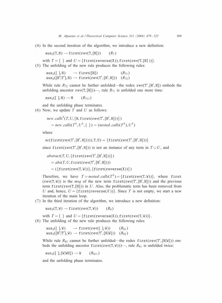
M. Alpuente et al. / Theoretical Computer Science 311 (2004) 479–525 509
(4) In the second iteration of the algorithm, we introduce a new deJnition:
aux2(T; H) → first(rev(T; [H])) (R7)
with T = { } and U = {first(reverse(X)); first(rev(T; [H]))}.(5) The unfolding of the new rule produces the following rules:
aux2([ ]; H) → first([H]) (R71)aux2([H′|T′]; H) → first(rev(T′; [H′; H])) (R72)
While rule R72 cannot be further unfolded—the redex rev(T′; [H′; H]) embeds theunfolding ancestor rev(T; [H]))—, rule R71 is unfolded one more time:
aux2([ ]; H) → H (R711)
and the unfolding phase terminates.(6) Now, we update T and U as follows:
new calls](T; U; {H; first(rev(T′; [H′; H]))})
= new calls(T]; U]; { }) = (nested calls(T]); U ])
where
nc(first(rev(T′; [H′; H])))); T; U) = {first(rev(T′; [H′; H]))}since first(rev(T′; [H′; H])) is not an instance of any term in T ∪U , and
abstract(T; U; {first(rev(T′; [H′; H]))})
= abs(T; U; first(rev(T′; [H′; H])))
= ({first(rev(T; W))}; {first(reverse(X))})
Therefore, we have T = nested calls(T]) = {first(rev(T; W))}, where first(rev(T; W)) is the msg of the new term first(rev(T′; [H′; H])) and the previousterm first(rev(T; [H])) in U . Also, the problematic term has been removed fromU and, hence, U = {first(reverse(X ))}. Since T is not empty, we start a newiteration of the main loop.
(7) In the third iteration of the algorithm, we introduce a new deJnition:
aux3(T; W) → first(rev(T; W)) (R8)
with T = { } and U = {first(reverse(X)); first(rev(T; W))}.(8) The unfolding of the new rule produces the following rules:
aux3([ ]; W) → first(rev([ ]; W)) (R81)aux3([H′|T′]; W) → first(rev(T′; [H|W])) (R82)
While rule R82 cannot be further unfolded—the redex first(rev(T′; [H|W])) em-beds the unfolding ancestor first(rev(T; W)))—, rule R81 is unfolded twice:
aux3([ ]; [W|WS]) → W (R811)
and the unfolding phase terminates.

510 M. Alpuente et al. / Theoretical Computer Science 311 (2004) 479–525
(9) Now, we update T and U as follows:
new calls](T; U; {W; first(rev(T′; [H|W]))})
= new calls(T]; U]; { }) = (nested calls(T]); U ])
where
nc(first(rev(T′; [H|W])); T; U) = { }since first(rev(T′; [H|W])) is an instance of first(rev(T; W)) in U . Therefore,T and U are not changed and the main loop terminates.
(10) Finally, we fold the instances U = {first(reverse(X)); first(rev(T; W))} inrules R1, R612, and R82 using rules R6 and R8: 5
last(X) → aux1(X) (R1f)aux1([H|T]) → aux3(T; [H]) (R612f)aux3([H′|T′]; W) → aux3(T′; [H|W]) (R82f)
and the algorithm terminates.
The Jnal program of the transformation is as follows:
last(X) → aux1(X) (R1f)aux1([ ]) → first([ ]) (R611)aux1([H|T]) → aux3(T; [H]) (R612f)aux3([ ]; [W|WS]) → W (R811)aux3([H′|T′]; W) → aux3(T′; [H|W]) (R82f)
together with the deJnitions of first, reverse, rev, and aux2. Let us note that thisis a diGcult example where several transformation strategies fail to terminate due tothe use of an accumulating parameter in function rev.
Let us conclude this section by discussing some related work. The compositionalgorithm presented in this section shares many similarities with partial evaluationalgorithms for functional logic programs (e.g., [5,6]). In fact, the narrowing-drivenapproach to partial evaluation is able to achieve deforestation, similarly to positivesupercompilation [45] of functional programs or conjunctive partial deduction [21] oflogic programs. Our composition algorithm is as powerful as the narrowing-drivenpartial evaluator of [6] regarding the composition of nested function calls. Indeed,the main diNerence between these techniques lies in the fact that in the compositionalgorithm we only consider the generation of new functions for those terms that containnested function calls. Apart from this diNerence, both techniques perform the same basicsteps: a main loop consisting in introducing new, residual deJnitions and unfoldingthese deJnitions, followed by a Jnal folding phase. Moreover, both techniques employthe same control strategies to ensure the termination of the process: the embeddingordering and the operator msg. This means that our composition algorithm is alsocomparable to positive supercompilation or conjunctive partial deduction regarding theability to perform deforestation.
5 We ignore the rules for aux2 since they are not needed anymore due to the generalization process.

M. Alpuente et al. / Theoretical Computer Science 311 (2004) 479–525 511
5.2. Tupling
While other transformation techniques (like partial evaluation or composition) havebeen widely investigated, tupling is a less known—but equally powerful—transfor-mation strategy based on the fold=unfold methodology. The tupling strategy was orig-inally introduced in [14,20] to optimize functional programs. Essentially, it proceedsby grouping calls with common arguments together so that their results are computedonly once. When the strategy succeeds, multiple traversals of data structures can beavoided, thus transforming a non-linear recursive program into a linear recursive one[41]. Unfortunately, the tupling strategy is more involved than the composition strategy.It often requires complex analyses in order to extract appropriate tuples of calls to begrouped together [15], to guarantee termination on non-trivial classes of programs (e.g.,the synchronization analysis in [17]). The development of a fully automatic tupling al-gorithm is out of the scope of this paper. In the following, we develop the backboneof the tupling strategy in our setting, and illustrate its use by means of an example.
The input to the tupling strategy is a program containing a rule, l→ r, whoseright-hand side has the form r = r[ek ]Pk
, where r|p = ei for all p∈Pi, i= 1; : : : ; k, ande1; : : : ; ek are operation-rooted terms which share, at least, one variable x. Then, thestrategy proceeds in four transformation phases:
Eureka generation. First, we introduce a new rule of the form:
aux(x; y1; : : : ; yn) → 〈e1; : : : ; ek〉where Var(e1; : : : ; ek) = {x; y1; : : : ; yn} and x∈Var(ei) for all i= 1; : : : ; k.
Unfolding. Here, similarly to the composition strategy, we apply unfolding steps untilwe reach a right-hand side containing instances of e1; : : : ; ek (if possible) or stop theunfolding process if there is a risk of non-termination. If the process succeeds, weend up with a rule of the form:
aux(t0; t1; : : : ; tn) → �(C′[ek ]Qk)
for some substitution � and context C′.Abstraction. By using abstraction, the above rule is transformed into
aux(t0; t1; : : : ; tn) → �(C′[zk ]Qkwhere 〈z1; : : : ; zk〉 = 〈e1; : : : ; ek〉)
where z1; : : : ; zk are fresh variables. A similar transformation is applied to the originalrule l→r:
l → r[zk ]Pkwhere 〈z1; : : : ; zk〉 = 〈e1; : : : ; ek〉
Folding. Finally, we apply folding steps in order to transform the above rules as fol-lows:
l → r[zk ]Pkwhere 〈z1; : : : ; zk〉 = aux(x; y1; : : : ; yn)
aux(t0; t1; : : : ; tn) → �(C′[zk ]Qkwhere 〈z1; : : : ; zk〉 = aux(x; y1; : : : ; yn))

512 M. Alpuente et al. / Theoretical Computer Science 311 (2004) 479–525
The following example illustrates the tupling strategy. Consider the function fib tocompute the Fibonacci numbers:
fib(0) → s(0) (R1)fib(s(0)) → s(0) (R2)fib(s(s(X))) → fib(s(X)) + fib(X) (R3)
This is a typical function which has an exponential complexity that can be reducedto a linear one by applying the tupling strategy. The process starts by introducing thefollowing deJnition:
aux(X) → 〈fib(s(X)); fib(X) (R4)
Now, by unfolding the redex fib(s(X)) of rule R4 we get:
aux(0) → 〈s(0); fib(s(0))〉 (R41)aux(s(X)) → 〈fib(s(X)) + fib(X); fib(s(X))〉 (R42)
We unfold once again rule R41 in order to remove the call to fib:
aux(0) → 〈s(0); s(0)〉 (R411)
Then, abstraction is applied to rules R3 and R42 as follows:
fib(s(s(X))) → Z1 + Z2 where 〈Z1; Z2〉 = 〈fib(s(X)); fib(X)〉 (R3a)aux(s(X)) → 〈Z1 + Z2; Z1〉 where 〈Z1; Z2〉 = 〈fib(s(X)); fib(X)〉 (R42a)
Finally, the right-hand sides of both rules are folded using the original deJnition offunction aux:
fib(s(s(X))) → Z1 + Z2 where 〈Z1; Z2〉 = aux(X) (R3af )aux(s(X)) → 〈Z1 + Z2; Z1〉 where 〈Z1; Z2〉 = aux(X) (R42af )
Therefore, the transformed (linear) deJnition of function fib is as follows:
fib(0) → s(0) (R1)fib(s(0)) → s(0) (R2)fib(s(s(X))) → Z1 + Z2 where 〈Z1; Z2〉 = aux(X) (R3af )aux(0) → 〈s(0); s(0)〉 (R411)aux(s(X)) → 〈Z1 + Z2; Z1〉 where 〈Z1; Z2〉 = aux(X) (R42af )
As we mentioned before, the diGcult part of the tupling algorithm is the extraction ofappropriate tuples of program calls. For this purpose, we could adapt existing tuplinganalyses for functional programs like those presented in [15,17].
This is an interesting topic for further research. Some preliminary results can befound in [38]. In this proposal, all nested function calls are supposed to be Jrst (suc-cessfully) optimized by composition so that the considered program only containsnon-nested function calls. This restriction greatly simpliJes both the eureka genera-tion phase and the unfolding process (in particular, it helps to stop the unfolding offunction calls).

M. Alpuente et al. / Theoretical Computer Science 311 (2004) 479–525 513
6. The transformation system SYNTH
The basic rules presented so far have been implemented by a prototype system SYNTH
[2], which is publicly available at
http://www.dsic.upv.es/users/elp/soft.html
It includes a parser for the language Curry, a modern multi-paradigm declarative lan-guage based on needed narrowing which extends Haskell with features from logic andconcurrent programming [25,27]. It also includes a fully automatic composition strategybased on some (seemingly reasonable) heuristics.
The SYNTH system is written in SICStus Prolog v3.6 and the complete implementa-tion consists of about 680 clauses (2450 lines of code). The transformer is expressedby 330 clauses (including the user interface and the code needed to handle the groundrepresentation), the parser and other utilities by 190 clauses, needed narrowing is im-plemented by 90 clauses and deJnitional trees are constructed by means of 70 clauses.The implementation only considers unconditional programs. Conditional programs aretreated by using the predeJned functions and, if then else, and case of, which arereduced by standard deJning rules (see, e.g., [39]).
Language syntax follows mainly that of the language Curry. Programs consist of aset of datatype and function declarations. For instance, the datatype declarationdata treeInt = Leaf Int
| Tree treeInt Int treeIntintroduces the datatype treeInt of binary trees whose nodes are labelled with integers.
A function is deJned by a list of deJning equations. For instance, the functiondeclarationappend [] y = yappend (x:xs) y = x : append xs y
deJnes the well-known concatenation of lists.The main diNerences w.r.t. the standard Curry syntax (as deJned in [25]) are the
following:• conditional equations are not allowed;• variables begin with an uppercase and (constructor and deJned) functions begin with
a lowercase (as in Prolog);• type declarations for deJned functions are not allowed (SYNTH does not include type
checking);• the let construction is not allowed, although local declarations can be given using
the where construction.We have recently incorporated a graphical interface (written in Java) to the systemthat enhances the interaction with the user. The SYNTH main screen is divided into fourareas, as shown in Fig. 4:
(1) In the upper row of the screen, a toolbar presents the following options:
(a) File: contains the typical options for opening, loading and saving a Jle, aswell as cleaning and exiting the system.

514 M. Alpuente et al. / Theoretical Computer Science 311 (2004) 479–525
Fig. 4. Folding transformation in the SYNTH environment.
(b) Edit: apart from the facilities for cutting, copying, pasting, Jnding and re-placing, it is possible to syntactically analyze a program and to show=edit anyprogram in a given transformation sequence; also, the system is able to showthe deJnitional trees for each deJned function symbol in the program.
(c) Rules: allows the user to apply any of the transformation rules presented inSection 3.
(d) Strategies: starts the application of the composition—in both an automaticor semiautomatic way—and tupling strategies.
(e) Options: for conJguring visual features of the system, like colors, fonts, etc.(f) Help: contains additional information about the system.
(2) The edit window appears in the central area of the screen. In this window, it is pos-sible to simultaneously edit diNerent programs belonging to a given transformationsequence, as shown in Fig. 4.
(3) The messages window appears below the previous one, and it is used by the systemto show information about the operation that is being performed (parsing, folding,etc.).
(4) Finally, the right column of the screen is used for dynamically listing the set ofallowed options during a transformation process. This facility displays the sequenceof applicable icons that can also be selected (in a less direct way) through the

M. Alpuente et al. / Theoretical Computer Science 311 (2004) 479–525 515
toolbar. For instance, the icon associated to the unfolding rule only appears whena rule has been marked inside a loaded program.
The system automatically assigns a number (starting from 0) to each program gener-ated in a transformation sequence. Program rules are also numbered and labelled withthe name of the transformation rule that produced them. Hence, it is easy to identifythe sequence of transformation steps performed along a transformation process as wellas to visualize the sequence of programs by simply clicking one of the options (First,Previous, Next, Last or Go to) which are shown between the edit window and themessages window. In Fig. 4, a folding operation has just been performed using tworules belonging to diNerent programs (dapp 5 and dapp 1, respectively). In this ex-ample, an additional window is displayed (right-down corner) which shows the foldedand folding program rules involved in the transformation.
As for transformation heuristics, SYNTH includes a fully automatic composition strat-egy based on some (apparently eNective) heuristics. We plan to extend it in order toalso deal with tupling automatically (by using, e.g., the analysis method of [15]).
The transformation system allows us to choose between two diNerent heuristics toachieve composition. The Jrst strategy (option comp) is semi-automatic: the user isasked to select the rule where the considered nested call appears, and has to providealso an initial deJnition rule for the transformation to start. The second strategy (optionacomp) is completely automatic: Jrst a nested call within the program is automaticallychosen and, then, an appropriate deJnition rule for a new function is introduced. Afterthese initial actions, the system proceeds automatically in both strategies. SYNTH buildsan incomplete, Jnite search tree, while looking for a node which can deliver a recursivedeJnition of the new function by a Jnal folding step. Finiteness is ensured either byimposing depth-bounds to the tree or by means of the (homeomorphic) embeddingtest on comparable ancestors of selected redexes. This expands derivations while newredexes are less than previous comparable redexes (i.e., with the same root functionsymbol) appeared in the same branch (using the homeomorphic embedding ordering).Once the required node is found, the original rule is replaced by the transformed one;otherwise, the set of unfoldings which correspond to the non-failed branches of thetree is returned.
Table 1 summarizes our benchmark results. The Jrst two columns measure the num-ber of rewrite rules (Rw1) and the absolute runtimes (RT1) for the original programs.The other columns show the number of rewrite rules (Rw2)—which includes the rulesof the original program since we apply no deJnition elimination steps—, the absoluteruntimes (RT2), and the speedups achieved for the transformed programs (we includeboth the speedup factor RT1=RT2 and the percentage ((RT1 − RT2)=RT1) × 100). Allthe programs have been executed by using the Curry environment PAKCS [26], whichcompiles Curry programs to Prolog. Times are expressed in milliseconds and are theaverage of 10 executions (for suGciently large input goals).
Our (automatic) composition strategy performs well w.r.t. the Jrst four benchmarks,which are typical functional programs to illustrate deforestation [48]: dapp and sum-prefix are described in Section 5, while the source code of lengthapp and double-flip are listed in Table 2. In these examples, composition is able to perform an

516 M. Alpuente et al. / Theoretical Computer Science 311 (2004) 479–525
Table 1Benchmark results
Programs Rw1 RT1 Rw2 RT2 RT1=RT2 Speedups
doubleappend 3 1320 6 1190 1.109 9.8%sumprefix 4 1850 6 1030 1.796 44.3%lengthapp 5 1090 7 980 1.112 10.1%doubleflip 3 1520 5 1400 1.086 7.9%fibonacci 3 1410 5 400 3.525 71.6%factlist 4 1480 6 245 6.040 83.4%average 5 1430 7 1080 1.324 24.5%
Table 2Original and transformed source programs
Lengthapp After composition
lengthapp(L1, L2) → len(app(L1, L2)) lengthapp(L1, L2) → new(L1, L2)len(nil) → 0 new(nil,L) → len(L)len(H:T) → s(len(T)) new(H:T,L) → s(new(T,L))app(nil,L) → Lapp(H:T, L) → H:app(T,L)
doubleflip After composition
Doubleflip(T) → f(f(T)) doubleflip(T) → n(T)f(leaf(N)) → leaf(N) n(leaf(N)) → leaf(N)f(tree(L,N,R) → tree(f(R); N,f(L)) n(tree(L,N,R) → tree(n(L),N,n(R))
factlist After tupling
flist(0) → nil flist(0) → nilflist(s(N)) → fact(s(N)) : flist(N) flist(s(N)) → U:V where 〈U,V〉= n(N)fact(0) → 1fact(s(N)) → s(N)*fact(N) n(0) → 〈s(0); nil〉
n(s(N)) → 〈s(s(N)) ∗ U,U:V〉 where 〈U,V〉= n(N)
Average After tupling
average(L) → sum(L)/length(L) average(L) → U/V where 〈U,V〉= new(L)sum(nil) → 0sum(H:T) → H + sum(T) new(nil) → 〈0,0〉length(nil) → 0 new(H:T) → 〈H+U,s(V)〉 where 〈U,V〉= new(T)length(H:T) → s(length(T))
eNective optimization (with speedups ranging between 7.9% and 44.3%). Regardingthe last three benchmarks, fibonacci has already been described in Section 5 whilefactlist and average are shown in Table 2. In all these cases a tupling strategywas necessary to succeed, as expected. As Table 1 shows, the tupling strategy obtains

M. Alpuente et al. / Theoretical Computer Science 311 (2004) 479–525 517
better eGciency improvements w.r.t. the composition strategy (with speedups rangingbetween 24:5% and 83:4%) although, in this case, the transformation sequence mustbe guided by the user.
In general, transformed programs cannot be guaranteed to be faster than the originalones, since there is a trade-oN between the smaller amount of computation neededafter the transformation (when guided by appropriate strategies) and the larger numberof derived rules. Nevertheless, our experiments seem to substantiate that the smallercomputations make up for the overhead of checking the applicability of the largernumber of rules.
7. Conclusions
The deJnition of a fold=unfold framework for the optimization of functional logicprograms was an open problem marked in [41] as pending research. We have pre-sented a transformation methodology for lazy functional logic programs preserving thesemantics of both values and answers computed by an eGcient (currently the best)operational mechanism. For proving correctness, we extensively exploit the existingresults from Huet and Levy’s theory of needed reductions [28] and the wide literatureabout completeness of needed narrowing [9] (rather than striving an ad-hoc proof). Wehave shown that the transformation process keeps the inductively sequential structureof programs. We have also shown that the transformation process can be guided byappropriate strategies which lead to eNective improvements. The experiments show thatour transformation framework combines in a useful and eNective way the systematicinstantiation of calls during unfolding (by virtue of the logic component of the needednarrowing mechanism) with the power of the abstraction transformations (thanks tothe functional dimension). We have also presented an implementation which allowsus to perform automatically the composition strategy as well as to perform all basictransformations in a semi-automated way. The results of this work can be applied tooptimize a large class of kernel (i.e., non-concurrent) Curry programs.
Acknowledgements
We thank Ivan Ziliotto and C(esar Ferri for having implemented the transformerSYNTH and for the evaluation of the benchmarks. We thank the anonymous refereesfor their accurate and useful remarks and suggestions, which helped to improve ourpaper.
Appendix A. Proof of Theorem 11
First, we state that transformation sequences preserve the inductively sequential struc-ture of programs. In order to prove it, we need the following technical results from

518 M. Alpuente et al. / Theoretical Computer Science 311 (2004) 479–525
[6]. The Jrst proposition shows that each substitution in a needed narrowing step in-stantiates only variables occurring in the initial term.
Proposition A.1 (Alpuente et al. [6]). If (p; R; ’k ◦ · · · ◦’1)∈ %(t;P) is a needednarrowing step, then, for i= 1; : : : ; k; ’i = id or ’i = {x �→ c(xn)} (where xn are pair-wise di>erent variables) with x∈Var(’i−1 ◦ · · · ◦’1(t)).
The following lemma shows that, for diNerent narrowing steps (computing diNerentsubstitutions), there is always a variable which is instantiated to diNerent constructors:
Lemma A.2 (Alpuente et al. [6]). Let t be an operation-rooted term, P a de7nitionaltree with pattern(P)6t and (p; R; ’k ◦ · · · ◦’1); (p′; R′; ’′
k′ ◦ · · · ◦’′1)∈ %(t;P);
k6k ′. Then, for all i∈{1; : : : ; k},• either ’i ◦ · · · ◦’1 =’′
i ◦ · · · ◦’′1, or
• there exists some j¡i with(1) ’j ◦ · · · ◦’1 =’′
j ◦ · · · ◦’′1, and
(2) ’j+1 = {x �→ c(· · ·)} and ’′j+1 = {x �→ c′(· · ·)} with c = c′.
Finally, we proceed with the proof of Theorem 11, which states that transformationsequences preserve the inductively sequential structure of programs.
Theorem 11. Let (R0; : : : ;Rn), n¿0, be a transformation sequence such that R0 isan inductively sequential program. Then, Ri is inductively sequential, for i= 1; : : : ; n.
Proof. We prove the claim by induction on i. Since the case i= 0 is obvious, weproceed with the inductive case. By the induction hypothesis, we have that Ri−1 isinductively sequential. Then, for every deJned function symbol f=n in Ri−1, thereexists a deJnitional tree of f in Ri−1. Now we prove that this result also holds inRi. We distinguish the following cases depending on the transformation rule appliedto Ri−1:De�nition introduction. By DeJnition 3, the program Ri has been obtained by adding
to program Ri−1 a new rule of the form R= (f(tn)→ r), such that f is a newfunction symbol not occurring in the sequence R0; : : : ;Ri−1 and f(tn) is a linearpattern. Trivially (see, e.g., [6]), a function deJnition which consists of a single rulewhose lhs is a linear pattern has always an associated deJnitional tree. Hence, theinductive sequentiality of Ri follows by the induction hypothesis.
De�nition elimination. By DeJnition 4, the program Ri has been obtained by deletingfrom program Ri−1 all rules in the deJnition of a given function f. Then, theinductive sequentiality of Ri follows trivially by the induction hypothesis.
Folding. By DeJnition 8, the program Ri has been obtained from Ri−1 by removinga rule R= (l→ r)∈Ri−1 and adding a new rule of the form R′ = (l→ r[�(l′)]p)(which cannot contain extra variables due to the restriction imposed in DeJnition 3).Since the left-hand sides of both programs Ri−1 and Ri coincide, the claim followsby the induction hypothesis.

M. Alpuente et al. / Theoretical Computer Science 311 (2004) 479–525 519
Unfolding. By DeJnition 5, the program Ri has been obtained from Ri−1 by removinga rule R= (l→ r)∈Ri−1 and adding a new set of rules of the form:
’1(l) → r1...’m(l) → rm
where r ❀’i ri, i= 1; : : : ; m, are all the one-step needed narrowing derivations issuingfrom r in Ri−1. Assume that l is rooted with the deJned function f, and f isdeJned in Ri−1 by a set of rules {Rj = (lj → rj) | j = 0; : : : ; n; n¿0}. By the inductionhypothesis, there exists a deJnitional tree P for f in Ri−1. Then, we know thatthe root of P is the pattern f(xp) (where p is the arity of f) and S = {l1; : : : ; ln}is the set of leaves of P, where obviously l∈ S and l ∈ P. In order to show theinductive sequentiality of Ri, it suGces to show that there exists a deJnitional treeP′ for the set
S ′ = (S\{l}) ∪ {’1(l); : : : ; ’m(l)}:
Consider for each needed narrowing step r ❀’i ri the associated canonical repre-sentation (p; R; ’iki ◦ · · · ◦’i1)∈ %(r;Pr) (where Pr is a deJnitional tree for the rootof r). Let
P′ = P ∪ {’ij ◦ · · · ◦ ’i1(l) | 1 6 i 6 m; 1 6 j 6 ki}:
We prove that P′ is a deJnitional tree for S ′ by showing that each of the fourproperties of a deJnitional tree holds for P′:
Root property: The minimum elements are identical for both deJnitional trees, thatis, pattern(P) =pattern(P′), since only instances of a leaf of P are addedin P′.
Leaves property: The maximal elements of P are S. Since all substitutions com-puted by needed narrowing along diNerent derivations are disjoint by Lemma A.2,the substitutions ’1; : : : ; ’m are pairwise disjoint. Thus, the replacement of theelement l in S by the set {’1(l); : : : ; ’m(l)} does not introduce any comparable(w.r.t. the subsumption ordering) terms. This implies that S ′ is the set of maximalelements of P′.
Parent property: Let $∈P′\{pattern(P′)}. We consider two cases for $:(1) $∈P: Then the parent property trivially holds since only instances of a leaf of
P are added in P′.(2) $ =∈ P: By deJnition of P′, $=’ij ◦ · · · ◦’i1(l) for some 16i6m and 16j6ki.
We show by induction on j that the parent property holds for $.Base case ( j = 1): Then $=’i1(l). It is ’i1 = id (otherwise $= l∈P). Thus,by Proposition A.1, ’i1 = {x �→ c(xn)} with x∈Var(r) ⊆ Var(l). Due to thelinearity of the initial pattern l and all substituted terms (cf. Proposition A.1),l has a single occurrence o of the variable x and, therefore, $= l[c(xn)]o, i.e.,l is the unique parent of $.
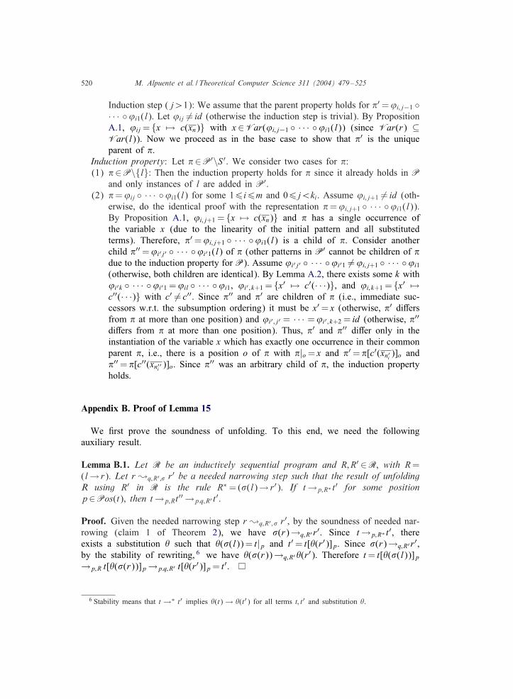
520 M. Alpuente et al. / Theoretical Computer Science 311 (2004) 479–525
Induction step ( j¿1): We assume that the parent property holds for $′ =’i; j−1 ◦· · · ◦’i1(l). Let ’ij = id (otherwise the induction step is trivial). By PropositionA.1, ’ij = {x �→ c(xn)} with x∈Var(’i; j−1 ◦ · · · ◦’i1(l)) (since Var(r) ⊆Var(l)). Now we proceed as in the base case to show that $′ is the uniqueparent of $.
Induction property: Let $∈P′\S ′. We consider two cases for $:(1) $∈P\{l}: Then the induction property holds for $ since it already holds in P
and only instances of l are added in P′.(2) $=’ij ◦ · · · ◦’i1(l) for some 16i6m and 06j¡ki. Assume ’i; j+1 = id (oth-
erwise, do the identical proof with the representation $=’i; j+1 ◦ · · · ◦’i1(l)).By Proposition A.1, ’i; j+1 = {x �→ c(xn)} and $ has a single occurrence ofthe variable x (due to the linearity of the initial pattern and all substitutedterms). Therefore, $′ =’i; j+1 ◦ · · · ◦’i1(l) is a child of $. Consider anotherchild $′′ =’i′j′ ◦ · · · ◦’i′1(l) of $ (other patterns in P′ cannot be children of $due to the induction property for P). Assume ’i′j′ ◦ · · · ◦’i′1 =’i; j+1 ◦ · · · ◦’i1
(otherwise, both children are identical). By Lemma A.2, there exists some k with’i′k ◦ · · · ◦’i′1 =’il ◦ · · · ◦’i1, ’i′ ; k+1 = {x′ �→ c′(· · ·)}, and ’i; k+1 = {x′ �→c′′(· · ·)} with c′ = c′′. Since $′′ and $′ are children of $ (i.e., immediate suc-cessors w.r.t. the subsumption ordering) it must be x′ = x (otherwise, $′ diNersfrom $ at more than one position) and ’i′ ; j′ = · · · =’i′ ; k+2 = id (otherwise, $′′
diNers from $ at more than one position). Thus, $′ and $′′ diNer only in theinstantiation of the variable x which has exactly one occurrence in their commonparent $, i.e., there is a position o of $ with $|o = x and $′ = $[c′(xn′i )]o and$′′ = $[c′′(xn′′i )]o. Since $′′ was an arbitrary child of $, the induction propertyholds.
Appendix B. Proof of Lemma 15
We Jrst prove the soundness of unfolding. To this end, we need the followingauxiliary result.
Lemma B.1. Let R be an inductively sequential program and R; R′ ∈R, with R=(l→ r). Let r ❀q;R′ ;� r′ be a needed narrowing step such that the result of unfoldingR using R′ in R is the rule R∗ = (�(l)→ r′). If t→p;R∗ t′ for some positionp∈Pos(t), then t→p;Rt′′ →p:q;R′ t′.
Proof. Given the needed narrowing step r ❀q;R′ ; � r′, by the soundness of needed nar-rowing (claim 1 of Theorem 2), we have �(r)→q;R′r′. Since t→p;R∗ t′, thereexists a substitution � such that �(�(l)) = t|p and t′ = t[�(r′)]p. Since �(r)→q;R′r′,by the stability of rewriting, 6 we have �(�(r))→q;R′�(r′). Therefore t = t[�(�(l))]p→p;R t[�(�(r))]p →p:q;R′ t[�(r′)]p = t′.
6 Stability means that t →∗ t′ implies �(t) → �(t′) for all terms t; t′ and substitution �.

M. Alpuente et al. / Theoretical Computer Science 311 (2004) 479–525 521
The soundness of the unfolding transformation can now be proved.
Lemma B.2. Let (R0; : : : ;Ri ;Ri+1); i¿0, be a transformation sequence such thatRi+1 has been obtained by unfolding, and let e be an equation. If e→∗true in Ri+1
then e→∗true in Ri.
Proof. We prove the claim by induction on the number n of rewrite steps in D= [e→∗
true]:Base case. Let n= 0. Then, we have e= true and the claim follows trivially.Inductive case. If n¿0 we have that D is not an empty reduction sequence. LetD= [e→p;R∗ e′ →∗ true]. If R∗ ∈Ri, then the claim follows by the inductive hy-pothesis. Otherwise, R∗ is the result of an unfolding transformation. In this case, byDeJnition 5, there are rules R= (l→ r); R′ ∈Ri such that r❀q;R′ ; � r′ is a needednarrowing step w.r.t. Ri and the result of unfolding R using R′ in Ri is the ruleR∗ = (�(l)→ r′)∈Ri+1. Moreover, there exists a substitution � such that e|p = �(�(l)). By Theorem 11, Ri is inductively sequential, and thus, by Lemma B.1, wehave
e →p;R e[�(�(r))]p →p:q;R′ e[�(r′)]p = e′
in Ri. Now, the claim follows by applying the inductive hypothesis to the derivatione′ →∗true in Ri+1.
Let us now consider the completeness of the unfolding rule. Firstly, we recall thenotion of descendant. Let A= (t→u;l→ r t′) be a reduction step of some term t into t′
at position u with rule l→ r. The set of descendants [28] of a position v of t by A,denoted v\A is
v\A =
∅ if u = v;{v} if u 6 v;{u:p′:q | r|p′ = x} if v = u:p:q and l|p = x; where x ∈ X:
The set of descendants of a position v by a reduction sequence B is deJned inductivelyas follows
v\B =
{v} if B is the null derivation;⋃w∈ v\B′
w\B′′ if B = B′B′′; where B′ is the initial step of B:
Given a set of positions P, we let P\B=⋃
p∈P p\B.A redex s in a term t is root-needed, if s (itself or one of its descendants) is
contracted in every rewrite sequence from t to a root-stable term [37]. In the remainderof this section, we consider it outermost-needed reduction sequences which are formallydeJned by means of the following function ’ from terms and deJnitional trees to sets

522 M. Alpuente et al. / Theoretical Computer Science 311 (2004) 479–525
of tuples (position, rule) as the least set satisfying the following properties. We considertwo cases for P:(1) If $ is a leaf, i.e., P= {$}, and $ → r is a variant of a rewrite rule, then
’(t;P) = {(�; $ → r)}:(2) If $ is a branch, consider the inductive position o of $ and some child $i =
$[ci(xn)]o ∈P. Let Pi = {$′ ∈P | $i6$′} be the deJnitional tree where all patternsare instances of $i. Then we consider the following cases for the subterm t|o:
%(t;P) �
(p; R) if t|o = ci(tn) and (p; R; �) ∈ %(t;Pi);(o:p; R) if t|o =f(tn) for f∈F and
(p; R) = ’(t|o;P′) where P′
is a deJnitional tree for f:
To compute outermost-needed steps for an operation-rooted term t, we take a deJ-nitional tree P for the root of t and compute ’(t;P). Then, for all (p; R)∈’(t;P),t →p;R t′ is an outermost-needed rewrite step. Outermost-needed reduction and needednarrowing are trivially equivalent for terms without variables.
We also need the following results from [6].
Theorem B.3 (Alpuente et al. [6]). Let R be an inductively sequential program. Let� be a substitution and V a 7nite set of variables. Let s be an operation-rooted termand Var(s) ⊆ V . Let �(s)→p1 ; R1 · · · →pn;Rn t be an outermost-needed rewrite sequencesuch that, for all root-needed redexes �(s)|p of �(s); p∈NVPos(s). Then, thereexists a needed narrowing derivation s ❀p1 ; R1 ; �1 · · · ❀pn;Rn; �n t
′ and a substitution �′
such that �′(t′) = t and �′ ◦ �n ◦ · · · ◦ �1 = �[V ].
Lemma B.4 (Alpuente et al. [6]). Let R be an inductively sequential program and tbe a term. If s is an operation-rooted subterm of t which contains a root-neededredex in t, then every outermost-needed redex of s is root-needed in t.
The following lemma is auxiliary.
Lemma B.5. Let R be an inductively sequential program and t be a term. Lett|p = �(l) be an innermost root-needed redex in t, where R= (l→ r)∈R; r is opera-tion-rooted, and p∈Pos(t). Given the reduction step A= [t→p;R t[�(r)]p], for everyoutermost-needed redex �(r)|q of �(r), we have p∈NVPos(r).
Proof. By contradiction. Assume that there exists an outermost-needed redex �(r)|qof �(r) and q =∈ NVPos(r). Since �(r) is operation-rooted and t|p is a root-neededredex in t, then �(r) must contain at least one root-needed redex in t. By Lemma B.4,�(r)|q is a root-needed redex in t. Let p′ ∈Pos(t) be a position such that q∈p′\A, i.e.,p′ is an antecedent of q w.r.t. A. Then, the subterm t|p′ , p¡p′, must be a root-neededredex in t, thus contradicting the hypothesis that t|p is an innermost root-needed redexin t.

M. Alpuente et al. / Theoretical Computer Science 311 (2004) 479–525 523
The following lemma states the completeness of the unfolding rule (at the level ofrewrite sequences). It essentially establishes that each rewrite sequence for an equationin the original program can be mimicked in the unfolded program.
Lemma B.6. Let (R0; : : : ;Ri ;Ri+1); i¿0, be a transformation sequence such thatRi+1 has been obtained by unfolding, and let e be an equation. If e→∗true in Ri
then e→∗true in Ri+1.
Proof. Let B1; : : : ; Bm be all possible needed reduction sequences from e to true, andlet ki be the number of contracted redexes in Bi, i= 1; : : : ; m. We prove the claim byinduction on the maximum number n=max(k1; : : : ; km) of contracted needed redexeswhich are necessary to reduce e to true:
n= 0. This case is trivial since e= true.n¿0. Since e contains at least one needed redex, then there exists a rule R= (l→ r) ∈
Ri such that e|p = �(l) is an innermost needed redex of e. Let us consider thefollowing reduction sequence
e →p;R e[�(r)]p →∗ true
in Ri. Now, if R belongs to both programs Ri and Ri+1, then the claim follows bythe inductive hypothesis.
Otherwise, R has been unfolded in Ri. Then, by DeJnition 5, the rhs r of therule R is not in head normal form and hence �(r) is an operation-rooted term. Let�(r)|q, q∈Pos(�(r)), be the outermost needed redex of �(r). By Lemma B.5, wehave that q∈Pos(r). Now, consider an arbitrary reduction step �(r)→q;R′r′; R′ ∈Ri,which contracts the outermost needed redex of r. Then, by Theorem B.3, the needednarrowing step r ❀q;R′ ; � r′′ can be proven in Ri, and there is a substitution �′ suchthat �′(r′′) = r′ and �′ ◦ �= �[Var(r)]. By DeJnition 5, the rule R∗ = (�(l)→ r′′)belongs to Ri+1 (i.e., it is the result of unfolding the rule R using R′).
Now, consider the reduction sequence
e →p;R e[�(r)]p →p:q;R′ e[r′]p →∗ true
in Ri. Finally, since the following step can be done in Ri+1 using the unfolded ruleR∗:
e = e[�(l)]p = e[�′(�(l))]p →p;R∗ e[�′(r′′)]p = e[r′]p
the claim follows by applying the inductive hypothesis to the subsequence e[r′]p →∗
true in Ri (whose maximum number of contracted needed redexes is strictly lesserthan n).Finally, Lemma 15 follows trivially by Lemmata B.2 and B.6.
References
[1] E. Albert, M. Hanus, G. Vidal, A practical partial evaluation scheme for multi-paradigm declarativelanguages, J. Funct. Logic Programming 2002 (1) (2002) 1–34.

524 M. Alpuente et al. / Theoretical Computer Science 311 (2004) 479–525
[2] M. Alpuente, M. Falaschi, C. Ferri, G. Moreno, G. Vidal, I. Ziliotto, The transformation system SYNTH.Technical Report DSIC-II/16/99, UPV, 1999. Accessible from URL: http://www.dsic.upv.es/users/elp/papers.html.
[3] M. Alpuente, M. Falaschi, G. Moreno, G. Vidal, Safe folding/unfolding with conditional narrowing, in:H. Heering, M. Hanus, K. Meinke (Eds.), Proc. Internat. Conf. on Algebraic and Logic Programming,ALP’97, Southampton (England), Lecture Notes in Computer Science, Vol. 1298, Springer, Berlin,1997, pp. 1–15.
[4] M. Alpuente, M. Falaschi, G. Moreno, G. Vidal, A transformation system for lazy functional logicprograms, in: A. Middeldorp, T. Sato (Eds.), Proc. 4th Fuji Internat. Symp. on Functional and LogicProgramming, FLOPS’99, Tsukuba (Japan), Lecture Notes in Computer Science, Vol. 1722, Springer,Berlin, 1999, pp. 147–162.
[5] M. Alpuente, M. Falaschi, G. Vidal, Partial evaluation of functional logic programs, ACM Trans.Programming Languages Systems 20 (4) (1998) 768–844.
[6] M. Alpuente, M. Hanus, S. Lucas, G. Vidal, Specialization of inductively sequential functional logicprograms, in: Proc. 4th ACM SIGPLAN Internat. Conf. on Functional Programming (ICFP’99), ACMSigplan Notices, Vol. 34.9, ACM Press, New York, 1999, pp. 273–283.
[7] S. Antoy, DeJnitional trees, in: Proc. 3rd Internat. Conf. on Algebraic and Logic Programming, ALP’92,Lecture Notes in Computer Science, Vol. 632, Springer, Berlin, 1992, pp. 143–157.
[8] S. Antoy, R. Echahed, M. Hanus, Parallel evaluation strategies for functional logic languages, in: Proc.14th Internat. Conf. on Logic Programming, ICLP’97, MIT Press, Cambridge, MA, 1997, pp. 138–152.
[9] S. Antoy, R. Echahed, M. Hanus, A needed narrowing strategy, J. ACM 47 (4) (2000) 776–822.[10] F. Baader, T. Nipkow, Term Rewriting and All That, Cambridge University Press, Cambridge, 1998.[11] R. Bol, Loop checking in partial deduction, J. Logic Programming 16 (1&2) (1993) 25–46.[12] A. Bossi, N. Cocco, Basic transformation operations which preserve computed answer substitutions of
logic programs, J. Logic Programming 16 (1993) 47–87.[13] M. Bruynooghe, D. De Schreye, B. Martens, A general criterion for avoiding inJnite unfolding, New
Generation Comput. 11 (1) (1992) 47–79.[14] R.M. Burstall, J. Darlington, A transformation system for developing recursive programs, J. ACM
24 (1) (1977) 44–67.[15] W. Chin, Towards an automated tupling strategy, in: Proc. Partial Evaluation and Semantics-Based
Program Manipulation, ACM, New York, 1993, pp. 119–132.[16] W. Chin, A. Goh, S. Khoo, ENective optimisation of multiple traversals in lazy languages, in: Proc.
Partial Evaluation and Semantics-Based Program Manipulation, San Antonio, Texas, USA (TechnicalReport BRICS-NS-99-1), University of Aarhus, DK, 1999, pp. 119–130.
[17] W.-N. Chin, S.-C. Khoo, T.-W. Lee, Synchronisation analysis to stop tupling, in: Proc. 7th EuropeanSymposium on Programming (ESOP’98), Lecture Notes in Computer Science, Vol. 1381, Springer,Berlin, 1998, pp. 75–89.
[18] B. Courcelle, Equivalences and transformations of regular systems—applications to recursive programschemes and grammars, Theoret. Comput. Sci. 42 (1986) 1–122.
[19] J. Darlington, An experimental program transformation and synthesis system, ArtiJcial Intelligence16 (1) (1981) 1–46.
[20] J. Darlington, Program transformation, in: J. Darlington, P. Henderson, D.A. Turner (Eds.), FunctionalProgramming and its Applications, Cambridge University Press, Cambridge, 1982, pp. 193–215.
[21] D. De Schreye, R. GlXuck, J. JHrgensen, M. Leuschel, B. Martens, M.H. SHrensen, Conjunctive partialdeduction: foundations, control, algorithms, and experiments, J. Logic Programming 41 (2&3) (1999)231–277.
[22] M.S. Feather, A survey and classiJcation of some program transformation approaches and techniques,in: IFIP 87, 1987, pp. 165–195.
[23] P.A. Gardner, J.C. Shepherdson, Unfold/fold transformation of logic programs, in: J.L Lassez, G. Plotkin(Eds.), Computational Logic, Essays in Honor of Alan Robinson, The MIT Press, Cambridge, MA, 1991,pp. 565–583.
[24] M. Hanus, The integration of functions into logic programming: from theory to practice, J. LogicProgramming 19&20 (1994) 583–628.

M. Alpuente et al. / Theoretical Computer Science 311 (2004) 479–525 525
[25] M. Hanus (Ed.). Curry: an integrated functional logic language, Available at http://www.informatik.uni-kiel.de/∼mh/curry/, 2003.
[26] M. Hanus, S. Antoy, J. Koj, R. Sadre, F. Steiner, PAKCS 1.5: The Portland Aachen Kiel Curry SystemUser Manual, Technical report, University of Kiel, Germany, 2003.
[27] M. Hanus, H. Kuchen, J.J. Moreno-Navarro, Curry: a truly functional logic language, in: Proc. ILPS’95Workshop on Visions for the Future of Logic Programming, 1995, pp. 95–107.
[28] G. Huet, J.J. L(evy, Computations in orthogonal rewriting systems, Part I + II, in: J.L. Lassez, G.D.Plotkin (Eds.), Computational Logic—Essays in Honor of Alan Robinson, The MIT Press, Cambridge,MA, 1992, pp. 395–443.
[29] T. Johnsson, Lambda lifting: transforming programs to recursive equations, in: Functional ProgrammingLanguages and Computer Architecture (Nancy, France), Lecture Notes in Computer Science, Vol. 201,Springer, Berlin, 1985, pp. 190–203.
[30] N.D. Jones, C.K. Gomard, P. Sestoft, Partial Evaluation and Automatic Program Generation,Prentice-Hall, Englewood CliNs, NJ, 1993.
[31] T. Kawamura, T. Kanamori, Preservation of stronger equivalence in unfold/fold logic programtransformation, Theoret. Comput. Sci. 75 (1990) 139–156.
[32] J.W. Klop, A. Middeldorp, Sequentiality in orthogonal term rewriting systems, J. Symbolic Comput. 12(1991) 161–195.
[33] L. Kott, Unfold/fold program transformation, in: M. Nivat, J.C. Reynolds (Eds.), Algebraic Methods inSemantics, Cambridge University Press, Cambridge, 1985, pp. 411–434.
[34] M. Leuschel, Homeomorphic embedding for online termination of symbolic methods, in: T. Mogensen,D. Schmidt, I.H. Sudborough (Eds.), The Essence of Computation—Essays Dedicated to Neil Jones,Lecture Notes in Computer Science, Vol. 2566, Springer, Berlin, 2002, pp. 379–403.
[35] M. Leuschel, B. Martens, D. De Schreye, Controlling generalization and polyvariance in partialdeduction of normal logic programs, ACM Trans. Programming Languages Systems 20 (1) (1998)208–258.
[36] M.J. Maher, A transformation system for deductive database modules with perfect model semantics,Theoret. Comput. Sci. 110 (2) (1993) 377–403.
[37] A. Middeldorp, Call by need computations to root-stable form, in: Proc. 24th Annu. ACMSIGPLAN-SIGACT Symp. on Principles of Programming Languages, ACM, New York, 1997,pp. 94–105.
[38] G. Moreno, Automatic optimization of multi-paradigm declarative programs, in: F.J. Garijo, J.C.Riquelme, M. Toro (Eds.), Proc. 8th Ibero–American Conf. on ArtiJcial Intelligence, IBERAMIA’02,Lecture Notes in ArtiJcial Intelligence, Vol. 2527, Springer, Berlin, 2002, pp. 131–140.
[39] J.J. Moreno-Navarro, M. Rodr()guez-Artalejo, Logic programming with functions and predicates: thelanguage Babel, J. Logic Programming 12 (3) (1992) 191–224.
[40] A. Pettorossi, M. Proietti, Transformation of logic programs: foundations and techniques, J. LogicProgramming 19,20 (1994) 261–320.
[41] A. Pettorossi, M. Proietti, Rules and strategies for transforming functional and logic programs, ACMComput. Sur. 28 (2) (1996) 360–414.
[42] D. Sands, Total correctness by local improvement in the transformation of functional programs, ACMTrans. Programming Languages Systems 18 (2) (1996) 175–234.
[43] W.L. Scherlis, Program improvement by internal specialization, in: Proc. 8th Annu. ACM Symp. onPrinciples of Programming Languages, ACM Press, New York, 1981, pp. 41–49.
[44] M.H. SHrensen, R. GlXuck, An algorithm of generalization in positive supercompilation, in: J.W. Lloyd(Ed.), Proc. ILPS’95, The MIT Press, Cambridge, MA, 1995, pp. 465–479.
[45] M.H. SHrensen, R. GlXuck, N.D. Jones, A positive supercompiler, J. Funct. Programming 6 (6) (1996)811–838.
[46] H. Tamaki, T. Sato, Unfold/fold transformations of logic programs, in: S. TXarnlund (Ed.), Proc. 2ndInternat. Conf. on Logic Programming, Uppsala, Sweden, 1984, pp. 127–139.
[47] P.L. Wadler, Listlessness is better than laziness, Ph.D. Thesis, Computer Science Department,CMU-CS-85-171, Carnegie Mellon University, Pittsburgh, PA, 1985.
[48] P.L. Wadler, Deforestation: transforming programs to eliminate trees, Theoret. Comput. Sci. 73 (1990)231–248.