roskilde university - core · roskilde university experimental master thesis in chemistry & ......
TRANSCRIPT
Roskilde University
Experimental Master Thesis in Chemistry &
Environmental Biology
Determination of organic matter decomposition rates in
Danish salt marsh sediment using novel analytical
chemical methods
Author:
Kristian Balling Hansen
Internal Supervisor:
Gary T. Banta
John Mortensen
External supervisor
Anne E. Giblin
January 2015 – April 2016

ii

iii
Abstract
Decomposition rates of organic matter in Danish salt marsh sediment were measured in this study
using a flow through reactor (FTR) experimental setup. Four different treatments using single and
multiple terminal electron acceptors (TEA) were prepared. One treatment was aerobic, whilst the
remaining were anaerobic. The consumption of different TEAs (nitrate, oxygen and sulfate) and
the production of carbon dioxide were measured over a period of 38 and 66 days in two
experiments. The mean (± SEM) nitrate consumption rate was 21.5 ± 3 nmol cm-3 h-1 when only
nitrate was available and 23.8 ± 3.48 nmol cm-3 h-1 when both nitrate and sulfate was available. The
mean (±SEM) oxygen consumption rate was 13.4 ± 0.88 nmol cm-3 h-1. Using both ion-
chromatography and a new method based upon precipitation of barium sulfate and flame atomic
absorption spectroscopy (fAAS) sulfate was analyzed. Neither of the two methods gave reliable
measurements of the sulfate consumption rate, however, as the deviations in the measurements
were greater than the changes due to consumption. The fAAS method does, however, hold a great
potential for situations where hundreds of samples needs to be analyzed but further investigation
is required before it can be implemented. To compare the different treatments carbon dioxide
production was measured. A new method for measuring carbon dioxide in aqueous solution was
developed. It uses a Gas Sensor Infrared electrode (GSIRe), and a custom apparatus. The method
was found to agree well with the already established Gran titration in the range of 0-5 mM CO���.
Using this new method, combined with the TEA consumption rates, dissolution of CaCO3 was
identified to contribute approximately 60 % of the total production of carbon dioxide. Despite this
contribution from the dissolution of CaCO3, the aerobic treatment used in the setup was over time
found to produce significantly more carbon dioxide than the two anaerobic treatments containing
either nitrate or sulfate as TEA. The daily production of carbon dioxide gave mean (± SEM) of the
aerobic treatment of 127.92 ± 3.38 nmol cm-3 h-1 whilst the treatments containing either sulfate or
nitrate gave 101.1 ± 2.96 and 94.66 ± 2.49, respectively. The treatment containing both nitrate and
sulfate had 117.51 ± 2.73 nmol cm-3 h-1. The decomposition rates were similar in the start of the
experiment for all treatments and over time the aerobic treatment become more productive than
the remaining treatments. The experimental evidence did support the idea that high levels of
nitrate would increase rates of salt marsh decomposition compared to sulfate reduction alone.
iv
Resume I dette studie blev nedbrydelsesraten af organisk materiale fra en dansk saltmarsk analyseret
gennem en eksperimentel opsætning med flow-through reaktorer (FTR). Fire forskellige
behandlinger hvor op til to terminale elektron acceptore (TEA) var benyttet. En af disse
behandlinger var aerob, mens de resterende tre var anaerobe. Forbruget af forskellige TEA’er
(nitrat, sulfat og oxygen) og produktion af carbondioxid var målt over en periode på 38 og 66 dage,
fordelt på to eksperimenter. Det gennemsnitlige forbrug af nitrat (±SEM) var 21.5 ± 3 nmol cm-3 h-1
når kun nitrat var tilsat behandlingen og 23.8 ± 3.48 nmol cm-3 h-1 når både sulfat og nitrat var
tilsat. Det gennemsnitlige forbrug af oxygen for den aerobe behandling (±SEM) var 13.4 ± 0.88
nmol cm-3 h-1. Sulfat blev analyseret ved brug af både ion-kromatografi og en ny metode baseret på
nedfældning af bariumsulfat og flamme atom absorption spektroskopi (fAAS). Ingen af de to
metoder medførte pålidelige resultater, idet afvigelserne i målingerne var større end det teoretiske
forbrug af sulfat. fAAS metoden har et stort potentiale i situationer hvor hundredevis af prøver
udføres, men flere undersøgelser er dog påkrævet før metoden kan implementeres. Til at
sammenligne de forskellige behandlinger imellem blev carbondioxid benyttet. En ny metode til at
måle carbondioxid i vandige opløsninger blev derfor udviklet. Denne nye metode bruger en gas
sensor med en infrarød elektrode (GSIRe) kombineret med et speciallavet apparat. Metoden
udviste samme nøjagtighed som en allerede etableret metode (Gran titrering) i området 0 – 5 mM
CO���. Ved brug af GSIRe og målingerne af forbrugsraterne fra de forskellige TEA’er, blev
opløseligheden af CaCO3 identificeret til at udgøre approksimativt 60% af den total produktion af
carbondioxid. På trods af denne ikke-biologiske produktion af carbondioxid blev den aerobe
behandling fundet til at producere signifikant mere carbondioxid over forløbet af eksperimentet
end de behandlinger som enten indeholdt sulfat eller nitrat. Den daglige produktion af
carbondioxid (±SEM), målt over alle dage for den aerobe behandling, var 127.92 ± 3.38 mens den
for behandlingen med enten nitrat eller sulfat var henholdsvis 101.1 ± 2.96 og 94.66 ± 2.49 nmol cm-
3 h-1. Behandlingen som indeholdt både nitrat og sulfat producerede 117.51 ± 27.31 nmol cm-3 h-1. I
starten af forsøget havde alle behandlingerne omtrent samme produktionsrater, men over tid blev
den aerobe behandling den mest produktive. Der var antydninger af, at høje nitrat niveauer ville
øge nedbrydningsraterne af saltmarsker, i forhold til hvis der kun var sulfat tilstede.

v
Preface This study was performed as an integrated master thesis (60 ECTS) in environmental biology and
chemistry at Roskilde University (RUC) from the 29th of January 2015 to the 29th of April 2016. The
thesis was carried out under internal supervision of associate professor John Mortensen and
associate professor Gary Thomas Banta from the department of Science and Environment at RUC
and external supervision of senior scientist Anne Giblin. The thesis investigates the aerobic and
anaerobic decomposition of organic matter in sediment from a typical Danish salt marsh using a
flow through reactor experimental setup. Analytical chemical methods for measuring carbon
dioxide and sulfate in aqueous solutions were modified, developed and verified. Decomposition
rates of the marsh sediment and the consumption rates of various terminal electron acceptors were
determined in two experiments.
Acknowledgements This thesis could not have been completed without involvement of several people. Thanks goes to
my supervisor Gary T. Banta for his help in developing the project idea, the long discussions at his
office, and support throughout the process. Thanks to my supervisor John Mortensen for his
tireless effort and aid in suggestions to the development of the analytical chemical section of the
thesis. Thanks to my external supervisor Anne E. Giblin for her helpful suggestions and feedback.
Thanks to laboratory technicians Rikke Guttesen, Gitte Katrine Bøg, Lone Thyboe Jeppesen,
Torben Brandt Knudsen and Anne Busk Faarborg for their immense help in the analysis of the
samples. For their friendly suggestions and support, I would like to thank Maria Bille, Jacob
Nepper-Davidsen, Camilla Knudsen and my family. Several people are not mentioned by name
but have contributed to this thesis and to whom I am deeply grateful for. Lastly, I would like to
thank the U.S. Sea Grant project, “The impacts of increased nitrogen loadings on decomposition in
salt marshes: Does eutrophication enhance marsh accretion or erosion?”, granted to Anne Giblin
and colleagues, which financially supported this project, especially in regards to construction of
the flow-through reactors used in this thesis.
vi
Table of contents
1. Introduction ............................................................................................................................................. 1
2. Theory ...................................................................................................................................................... 3
2.1 Sulfate measurements with atomic absorption spectrophotometry ....................................... 3
2.2 Measurement of ΣCO2 in a aqueous solution by a new method ............................................. 4
2.3 Aerobic and anaerobic decomposition of organic matter ......................................................... 6
3. Methods ................................................................................................................................................... 9
3.1 Flow through sediment reactor .................................................................................................... 9
3.2 Barium sulfate measurement by fAAS method ....................................................................... 11
3.3 Carbon dioxide measurement using the GSIRe method ......................................................... 12
3.4 Sampling sites ............................................................................................................................... 14
3.5 Preparation of the sediment and water for the treatments ..................................................... 15
3.6 Analysis of samples ...................................................................................................................... 19
3.7 Statistical analysis ......................................................................................................................... 20
4. Results .................................................................................................................................................... 20
4.1 Evaluation of the fAAS method .................................................................................................. 20
4.2 Evaluation of the GSIRe method for measuring carbon dioxide ........................................... 22
4.3 Sediment properties ..................................................................................................................... 30
4.4 Bromide experiment ..................................................................................................................... 32
4.5 Nitrate measurements .................................................................................................................. 36
4.6 Oxygen measurements ................................................................................................................ 37
4.7 Sulfate measurements .................................................................................................................. 38
4.8 Carbon dioxide production ......................................................................................................... 40
5. Discussion .............................................................................................................................................. 46
5.1. Experimental methods ................................................................................................................. 46
5.1.1. Sediment characteristics ...................................................................................................... 46
5.1.2. Flow through experiment .................................................................................................... 46
5.1.3. Measurements of nitrate ...................................................................................................... 48
5.1.4. Measurement of oxygen ...................................................................................................... 48
5.1.5. Measurement of sulfate........................................................................................................ 49
vii
5.1.6. Measurement of carbon dioxide ......................................................................................... 51
5.2. Consumption rates of various TEA ............................................................................................ 51
5.2.1. Nitrate consumption rate..................................................................................................... 51
5.2.2. Oxygen consumption rate ................................................................................................... 53
5.2.3. Sulfate consumption rate ..................................................................................................... 54
5.3. Daily carbon dioxide production rate ........................................................................................ 55
5.3.1. Carbon dioxide production from nitrate consumption ................................................... 55
5.3.2. Carbon dioxide production from oxygen consumption ................................................. 56
5.3.3. Carbon dioxide production from sulfate consumption .................................................. 56
5.3.4. Stoichiometry ........................................................................................................................ 56
5.3.5. Dissolution of CaCO3 ........................................................................................................... 57
5.3.6. Kinetics of CaCO3 ................................................................................................................. 60
5.3.7. Cumulative TEA production .............................................................................................. 61
6. Conclusion ............................................................................................................................................. 64
7. Reference list ......................................................................................................................................... 68

1
1. Introduction
Salt marshes are highly productive ecosystems located primarily at coastal estuaries or bar built
estuaries in the temperate region of the world (Vernberg 1993; Mann 2000). Usually found on
sheltered shores, the ecosystem constitute a region in the intertidal zone (Mann 2000).
Consequentially, salt marshes typically experience flooding twice a day. Over time, salt marshes
develops creeks and drainage channels, which transports and returns water to the sea (Mann
2000). The salt marsh is dependent on these flooding as they supply nutrients and allochthonous
inorganic material to the salt marsh. The development of plants enhances the deposit of the
allochthonous material, thus inducing an accretion of the salt marsh (Townend et al. 2011). For salt
marshes to persist over time, the sedimentation rates must equal or exceed the sea level rise
(Vernberg 1993). Salt marshes have been found to be vulnerable to nutrient loading (Deegan et al.
2012) and elevation in sea level (Morris et al. 2013) among other stressors. If the sea level rises with
more than a meter during the next 100 years there is a possibility that many salt marshes will be
permanently submerged (Kirwan et al. 2010). Salt marshes must elevate accordingly via salt marsh
accretion or they will be negatively affected (Anisfeld & Hill 2012). Salt marshes are somewhat
adaptable to these fluctuations in the sea level and addition of nutrients. The increase supply of
nutrients induces an increase in the biomass density and production that will enhance the trapping
of the sediment causing salt marshes to rise (Morris et al. 2002; Turner et al. 2009). The capacity of
salt marshes for accretion is not unlimited and Turner et al. (2009) demonstrated that nutrient
enrichment might lead to a significant loss of salt marsh. The natural change in the elevation of the
marsh is slow compared to the change in sea level that can happen within a year (Morris et al.
2002). If the plants experience flooding for a prolonged period, marsh drowning occurs.
Since the pre-industrial period the dissolved inorganic nutrient flux from anthropogenic sources to
the salt marshes have increased (Deegan et al. 2012). This increased addition of nutrients stimulate
the production of aboveground biomass (Valiela et al. 1976). Deegan et al. (2012) found, that with
higher nutrient availability, the root:shoot ratio decreases for smooth cordgrass, Spartina alterniflora
a dominant salt marsh species. In some studies this is only due to an increase in above ground
biomass, however, (Deegan et al. 2012) found in their study that there was a decrease in
belowground biomass. The new shoots contained less structural compounds, was taller, and

2
weighed more than the previous ones, resulting in a tendency for them to fall over. Due to the high
nitrogen content in the detritus and high availability of nitrate as electron acceptor the organic
matter decomposed quickly (Deegan et al. 2012). As time goes by, the remaining roots will become
exposed to erosion and storms, which will further cause harm (Darby & Turner 2008; Turner et al.
2009). It should be mentioned, however, that not all experiments support this hypothesis. Anisfeld
& Hill (2012) found, that neither nitrogen nor phosphorus fertilization lead to elevation loss.
Morris et al. (2013) discovered that the aboveground biomass increased after fertilization but was
unable to verify the effect of sediment organic matter and the strength of the sediment. It is
therefore ambiguous if addition of nutrient inevitable results in a loss of salt marsh as there are
evidence of both instances. Salt marshes are of utmost importance as the ecosystem provides
services for its inhabitants and the surrounding area. These services include, habitats for animals,
function as a carbon sink, protecting coastal cities from storms, prevention of floods, and nutrient
loadings from the surrounding areas, to mention a few (Deegan et al. 2012; Morris 1991; Turner et
al. 2009; Valiela & Cole 2002; Vernberg 1993).
If the sea level and addition of nutrients continues to increase, the decomposition of organic matter
will likely be influenced and hence the development of salt marshes. To evaluate the future of salt
marshes, further research is needed. One field that require attention is the importance of aerobic
and anaerobic decomposition rates of organic matter in salt marshes. Previously, it was thought
that breakdown of organic matter occurred through a thermodynamic ladder, in which the most
energetically favorable terminal electron acceptor (TEA) is consumed following the second most
favorable and so forth (Canfield et al. 2005). The ladder is now thought to be a simplistic version of
what occurs in the environment as it has been proven that mutual decompositions pathways can
occur (Bethke et al. 2011). Nevertheless, aerobic decomposition is the energetically most favorable
pathway, and it occurs in the top layer of the sediment but is not possible in the deeper layers in
shallow waters as the consumption exceeds the downward transport of oxygen (Kristensen 2000).
Anaerobic decomposition subsequently follow with nitrate and sulfate reducing decomposers
(Canfield et al. 2005). Nitrate and sulfate reduction rates in sediments have been compared by
several groups utilizing a flow through reactor (FTR) setup, but none of these measured the oxic
respiration (Laverman et al. 2006; Laverman et al. 2012; Pallud et al. 2007; Pallud & Van Cappellen

3
2006; Stam et al. 2011) Furthermore, not all groups utilized multiple TEAs in the treatments. In the
salt marsh ecosystem both sulfate, nitrate, and oxygen are readily available in the aqueous phase.
The decomposition rates and consumption rates obtained when analyzing one single TEA might
therefore not properly reflect the in situ rates.
The aim of this study is to establish a more profound understanding of the decomposition rates for
salt marsh detritus for different TEAs when both singly and multiple TEA were available for the
decomposers in ecologically relevant concentrations. This was accomplished by measuring the
different TEAs using a FTR experimental setup similar to Pallud et al. (2007). The utilized TEA
included not only nitrate and sulfate, but also oxygen in order to cover both aerobic and anaerobic
decomposition. Sediment from a Salt marsh in Emmerlev, a typical Danish salt marsh on the
Wadden Sea, was used and supplied with four different compositions of TEAs using a FTR
experimental setup. Carbon dioxide was measured and used to compare the decomposition rates
of the various treatments. In order to measure the production of carbon dioxide, a new method
was developed. Furthermore, an alternative method to measure sulfate in aqueous solutions is
presented in this study.
2. Theory
2.1 Sulfate measurements with atomic absorption spectrophotometry
Estimation of sulfate ions in various water sources are important in monitoring natural waters
(Burakham et al. 2004). Throughout the years, numerous methods have been developed to
determine sulfate concentrations for various purposes. These methods include i.a. colorimetric
(Bertolacini and Barney 1957), spectrophotometric (Roy et al. 2011; Gomes et al. 2014), turbidimetry
(Krug et al. 1977; Morais et al. 2003) and by ion-chromatograph (Morales et al. 2000).
An innovative method of determining sulfate obtained in the field based on solubility products
and flame atomic absorption spectroscopy (fAAS) is presented further in this study. The theory for
the method is presented in this section and is later in the study referred to as fAAS. The method,
relies upon precipitation of barium sulfate. The theory used for this method was grounded from

4
(Eq. 1) and (Eq. 2). The solubility product constant (Ksp) of barium sulfate is 1.1*10-10 M2 (Chang
2008).
Ba��(aq) + SO���(aq) ⇌ BaSO�(s) (Eq. 1)
K�� = �Ba����SO���� (Eq. 2)
An addition of a soluble barium chloride solution to a solution containing sulfate will, if the
product of the concentrations exceeds the solubility product constant, precipitate. When an excess
of barium is added to a solution, only a small percentage of the sulfate is soluble whilst the
remaining sulfate is lost as barium sulfate precipitate. The acidity of the solution affects the
composition of the precipitate. Carbonate and hydrogen sulfate can at specific pH ranges interfere
with the precipitation of barium sulfate (Morais et al. 2003). If carbonate is present, it can react
with the barium and precipitate as barium carbonate. To prevent this interference from these ions,
the solution was acidified. At pH values lower than four all bicarbonate and carbonate will be
driven out of the solution (confer (Eq. 5) and (Eq. 6)). If lower, the formation of bisulfate can lead to
underestimation of the sulfate in the solution. The pKa value of bisulfate is 1.88 (Chang 2008) and if
the pH of the solution was lower than three, some of the sulfate would be found as bisulfate
leading to an underestimation of the sulfate concentration in the original sample. The excess
barium is located in the supernatant and is measured using flame atomic absorption spectrum
(fAAS). An inverse relationship exists between barium and sulfate causing the barium
concentration to be high when sulfate was low in the solution.
2.2 Measurement of ΣCO2 in a aqueous solution by a new method
Reliable and precise measurements of carbon dioxide was crucial for understanding the
respiration occurring in the benthic environment. Other reports have used Gran titration for
estimating the concentration of carbon dioxide (Pallud et al. 2007; Kristensen 2000). Gran titration
uses diluted hydrogen chloride solution to titrate a specific volume of an aqueous sample. The
change in pH due to the acidification permits an estimation of the total carbon dioxide in the
sample based on measurements performed around the equivalence point of the sample of interest
(Gran 1952). This method is time consuming, not to mention labour demanding but produces
stable result. A new method for measuring carbon dioxide is presented in the following section of
5
this report. The theory underlying this method is based on acidification of an aqueous sample just
as Gran titration.
The equilibrium for carbon dioxide between being in the gaseous phase or dissolved in the liquid
is given in (Eq. 3). This relationship is dependent on the partial pressure (����) and the Henrys law
constant (����). The equilibrium constant for (Eq. 3) is equal to Henrys law constant.
CO�(aq) ⇆ H� � ∗ p� � (Eq. 3)
Gaseous carbon dioxide will after it dissolves, be hydrolyzed (Eq. 4). This reaction is independent
of the pH of the solution. It is instead dependent of the Henry's law constant and the partial
pressure of the gas. Henry’s law is affected by temperature, but this was regarded to be constant in
the following experiment as the measurement was executed in a climate chamber with a stable
temperature. Subsequently after the hydrolysis, it will further react with a water molecule
generating a hydrogen carbonate ion and a proton (Eq. 5). This hydrogen carbonate can be
removed of yet another proton (Eq. 6). Both reactions are strongly influenced by pH since a
decrease in pH will lead to a shift to the left in the reactions schemes and vice versa. If the solution
is very acidic, the largest proportion of the carbon dioxide will exist as CO� ∙ H�O. Because of this
the reaction will once again be shifted to the left and the dissolved carbon dioxide will become
gaseous (Seinfeld & Pandis 2006).
CO�(g) + H�O ⇆ CO� ∙ H�O (Eq. 4)
CO� ∙ H�O ⇆ HCO�� + H� (Eq. 5)
HCO�� ⇆ CO�
�� + H� (Eq. 6)
The pKa value for the (Eq. 5) is 6.38 and for (Eq. 6) is 10.319 (Chang 2008). The water used in the
experiment had reservoirs with a pH of 6.3 and in the outlet, a pH between 8-9.3 was measured.
The majority of the carbon dioxide will hence be present in the water as HCO�� . For dissolved
carbon dioxide under acidic solutions (pH < 5), most of it will hence be in the form of CO� ∙ H�O,
but above pH 5 the dissolved carbon dioxide increases exponentially (Seinfeld & Pandis 2006).
This theory paved the way for developing a procedure for the estimation of carbon dioxide in
aqueous solutions. By adding an excess of protons, the shift in pH of the solution lead to a reaction
where the hydrogen carbonate reacted with the proton producing carbon dioxide, thereby
6
increasing the concentration in the gas phase. A hermetic closed container confined the gas until an
equilibrium was obtained. A gas sensor using an IR electrode measured the gas (Vernier, carbon
dioxide gas senor). The method is later in this study referred to as Gas Sensor Infrared electrode
(GSIRe). The GSIRe method do not directly use pH as a way of measuring ΣCO2 as Gran titration
does. Instead, it measures the number of carbon dioxide molecules from a specific volume of a
solution that evaporates due to acidification of the sample. These apparent insignificant differences
permitted a reduction in the work required per sample.
2.3 Aerobic and anaerobic decomposition of organic matter
In salt marshes, the preservation of carbon is influenced by various factors. These include;
deposition rates of organic matter, organic carbon source, bacterial grazing, adsorption,
geopolymerization, and metabolite inhibition (Canfield 1994). At low sediment precipitation,
aerobic respires have a long period to decompose the organic material, and hence the oxidation of
carbon is occurring aerobic. At high deposition rates, the oxygen is rapidly exhausted and
anaerobic decomposition occurs. Preservation of carbon will occur, if the rates of decay are lower
than the rates for deposition of organic matter start to build up (Canfield 1994).
When sediment reaches the sea floor, the organic matter decomposes through various pathways
(Kristensen et al. 1995; Kristensen & Hansen 1995). If oxygen is available, all catabolic processes
will be aerobic (Canfield et al. 2005). The aerobic breakdown of the detritus commences by aerobic
microorganisms attaching themselves to organic particles. Excretion of substrate-specific cell
bound ectoenzymes or exoenzymes enable a breakdown of dissolved organic carbon (DOC), which
the microorganisms can assimilate (Canfield et al. 2005). Almost all aerobic microorganisms can
assimilate DOC and fully oxidize it to carbon dioxide, water, and inorganic nutrients (Canfield et
al. 2005; Canfield 1994; Kristensen et al. 1995; Kristensen and Holmer 2001). The process of aerobic
decomposition utilize enzymes together with reactive oxygen species (ROS) such as superoxide
anion (∙O��), peroxide (H�O�), and hydroxyl radicals (∙OH) for breakdown of different bonds. These
radicals are capable of reacting with sturdy bonds found such as those found in lignin and as a
result promote decomposition (Canfield 1994). Oxygen furthermore participate as a reactant in
opening ring structures (Canfield 1994; Kristensen et al. 1995). As oxygen is rapidly exhausted, it
7
does not penetrate further than a couple of mm down in productive shallow sediment (Hulthe et
al. 1998). This is a consequence of both the aerobic respires consuming the oxygen and oxygen
being used to re-oxidize products from the anaerobic respiration in the oxic/anoxic interface
(Hansen and Blackburn 1991). The limiting step for the aerobic decomposition is the initial
hydrolytic attack (Kristensen & Holmer 2001).
Beneath the oxic zone, the organic matter decomposes anaerobically. In contrast to aerobic
decomposition, anaerobic decomposition of organic matter cannot be accomplished by a single
bacterium, but instead have to be performed through the action of several (Canfield 1994;
Kristensen et al. 1995). The initial attack of the organic matter is through hydrolysis of molecules,
which split the molecule into smaller moieties. Hydrolytic/fermenting organisms secrete
ectoenzymes or exoenzymes causing a break in the detritus. The moieties are assimilated and
afterwards released. Fermenting organisms assimilate the released material and afterwards release
smaller parts of molecules. The released organic matter is small enough for prokaryotes to
dissimilate it to carbon dioxide using terminal electron acceptors (e.g nitrate, sulfate) (Canfield
1994; Kristensen et al. 1995). Each of these several organisms only get a fraction of the energy
available in the substrate before it is released (Canfield et al. 2005). Due to the lack of ROS, lignin
and other refractory material will under anaerobic conditions break down slower compared to
aerobic conditions (Canfield 1994). The limiting step for anaerobic decomposition is the initial
hydrolytic and fermentative attack (Kristensen et al. 1995; Kristensen & Holmer 2001).
The respiration for the different microorganisms occur in different zones in the sediment according
to the energy released in the process and availability of their electron acceptor (Canfield et al.
2005). These zones constitute a thermodynamic ladder in which electron acceptors are placed on
rungs accordingly to the Gibbs free energy (∆&') of the involved reaction (confer Table 1). This
way of presenting the electron acceptors is an oversimplification but provides a simple overview
of the succession of electron acceptors (Canfield et al. 2005). Hypothetically, the different terminal
electron acceptors use their energetic advantage to exclude less efficient terminal electron
acceptors (Bethke et al. 2011). Bethke et al. (2011) tested the theory of exclusion based on a
thermodynamical advantage for methagens, sulfate reducers, and iron reducers in the laboratory.
8
The group was unable to identify a hierarchy for methanogens, sulfate reducers, and iron reducers.
They argue that ecological factors such as population viability and mutualism, rather than
thermodynamics alone affect the microbial distribution in the laboratory and possibly the nature.
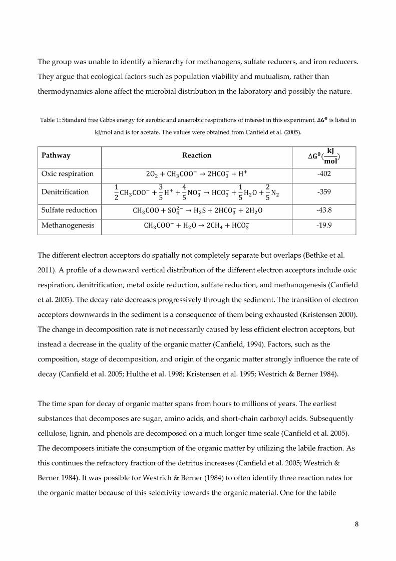
Table 1: Standard free Gibbs energy for aerobic and anaerobic respirations of interest in this experiment. ∆() is listed in
kJ/mol and is for acetate. The values were obtained from Canfield et al. (2005).
Pathway Reaction ∆*)(+,
-./)
Oxic respiration 2O� + CH�COO� → 2HCO�� + H� -402
Denitrification 12
CH�COO� +35
H� +45
NO�� → HCO�
� +15
H�O +25
N� -359
Sulfate reduction CH�COO + SO��� → H�S + 2HCO�
� + 2H�O -43.8
Methanogenesis CH�COO� + H�O → 2CH� + HCO�� -19.9
The different electron acceptors do spatially not completely separate but overlaps (Bethke et al.
2011). A profile of a downward vertical distribution of the different electron acceptors include oxic
respiration, denitrification, metal oxide reduction, sulfate reduction, and methanogenesis (Canfield
et al. 2005). The decay rate decreases progressively through the sediment. The transition of electron
acceptors downwards in the sediment is a consequence of them being exhausted (Kristensen 2000).
The change in decomposition rate is not necessarily caused by less efficient electron acceptors, but
instead a decrease in the quality of the organic matter (Canfield, 1994). Factors, such as the
composition, stage of decomposition, and origin of the organic matter strongly influence the rate of
decay (Canfield et al. 2005; Hulthe et al. 1998; Kristensen et al. 1995; Westrich & Berner 1984).
The time span for decay of organic matter spans from hours to millions of years. The earliest
substances that decomposes are sugar, amino acids, and short-chain carboxyl acids. Subsequently
cellulose, lignin, and phenols are decomposed on a much longer time scale (Canfield et al. 2005).
The decomposers initiate the consumption of the organic matter by utilizing the labile fraction. As
this continues the refractory fraction of the detritus increases (Canfield et al. 2005; Westrich &
Berner 1984). It was possible for Westrich & Berner (1984) to often identify three reaction rates for
the organic matter because of this selectivity towards the organic material. One for the labile

9
fraction (G1), one for the refractory fraction (G2) and lastly one for a fraction, which under oxic
decomposition was non-reactive (GNR) (Westrich & Berner 1984). The decomposition of the labile
fraction of the organic matter has been found to be similar when nitrate, oxygen, and sulfate were
consumed as an electron acceptors (Kristensen & Holmer 2001). Westrich & Berner (1984) found
using fresh plankton the half time for the labile fraction using sulfate reduction to be 10 days. The
stage of composition is vital for the aerobic and anaerobic decomposition. Generally, the fresher
and more labile the material is, the less difference there is in rate of decomposition for aerobic and
anaerobic (Hulthe et al. 1998).
3. Methods
3.1 Flow through sediment reactor
Most of the experimental data was obtained using a FTR experimental setup. Similar setups have
been used several times and described in details by various authors (Roychoudhury et al. 1998;
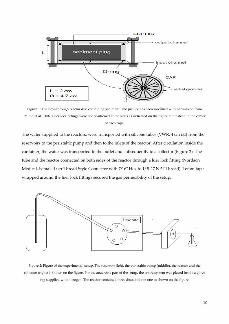
Pallud et al. 2007; Pallud & Van Cappellen 2006). The setup for the FTR consist of several parts
(Figure 1). The reactors, in which the sediment is located, consist of 20 mm Plexiglas cylinder discs
with an inner diameter of 47 mm (Figure 1). Two Plexiglas caps containing a groove, holds the
reactor in place. An O-ring inserted between the reactor and the groove permits a fastening of the
reactor and prevents leakage. GF/C filters (Whatman, 47mm) located at both ends of the reactor
prevent sediment from leaving the reactors. Radial groves located on the side of the caps at both
the inflow and outflow enabled a steady flow of water throughout the experiment. Nylon screws
holds the setup together. It proved necessary for these screws to generate an equal force of
pressure on the caps. If the pressure was uneven, the setup leaked and needed correction in the
tightening. This was accomplished through a trial and error process.
10
Figure 1: The flow-through reactor disc containing sediment. The picture has been modified with permission from
Pallud et al., 2007. Luer lock fittings were not positioned at the sides as indicated on the figure but instead in the center
of each caps.
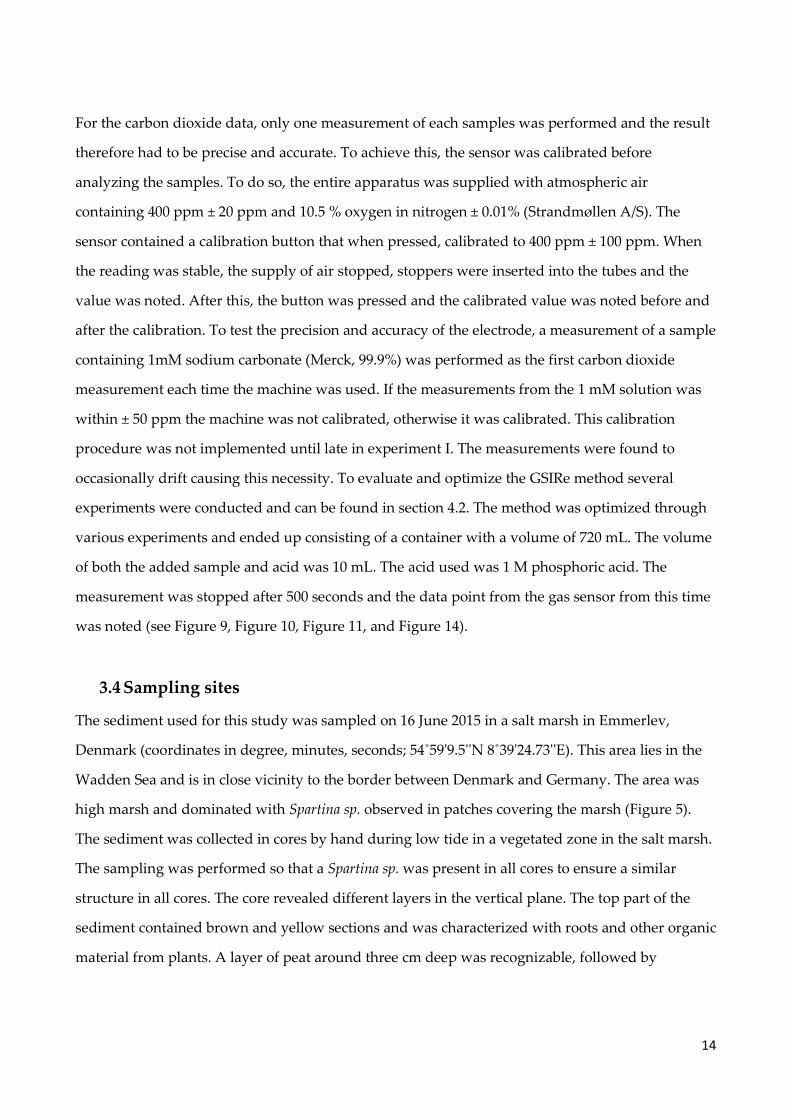
The water supplied to the reactors, were transported with silicone tubes (VWR, 4 cm i.d) from the
reservoirs to the peristaltic pump and then to the inlets of the reactor. After circulation inside the
container, the water was transported to the outlet and subsequently to a collector (Figure 2). The
tube and the reactor connected on both sides of the reactor through a luer lock fitting (Nordson
Medical, Female Luer Thread Style Connector with 7/16" Hex to 1/ 8-27 NPT Thread). Teflon tape
wrapped around the luer lock fittings secured the gas permeability of the setup.
Figure 2: Figure of the experimental setup. The reservoir (left), the peristaltic pump (middle), the reactor and the
collector (right) is shown on the figure. For the anaerobic part of the setup, the entire system was placed inside a glove
bag supplied with nitrogen. The reactor contained three discs and not one as shown on the figure.

11
To obtain stable measurements using a FTR several conditions must be fulfilled. The concentration
of the reactant measured in the outlet must be sufficiently high to ensure that a complete
consumption did not occurred (Pallud et al. 2007). On the other hand, the time inside the container
(the fluid residence time) has to be long enough for a measureable change in concentration in the
in- and outflow of water to occur (Roychoudhury et al. 1998). Both scenarios can be accomplished
by changing the flow rate, the supplied reactant concentration or both (Pallud et al. 2007). The
supplied water has to be supplied uniformly to the entire reactors. This is to avoid areas in the
reactors from differentiating in their activity. This was investigated by the use of an inert tracer, in
this study bromide and by visual inspection of the colour of the sediment.
3.2 Barium sulfate measurement by fAAS method
As mentioned in the theory section of this study, this thesis present a new method of measuring
sulfate in aqueous solutions. The new method revolves around usage of flame atomic absorption
spectroscopy. The fAAS method of measuring sulfate consisted of four steps (Figure 3). To a
reagent glass 2 mL sample containing sulfate, 2 mL barium chloride (36.58 mM), and hydrogen
chloride (0.5 M) was transferred resulting in precipitation of barium sulfate. The barium
concentration was in a large excess compared to the sulfate (the concentration in the reservoir were
22.5 mM) meaning that virtually all sulfate precipitates, whilst the remaining barium is in the
supernatant (A). Subsequently the prepared samples were transferred to the refrigerator and
cooled for a day. The cooling step was implemented as the initial experiments had proved that
initial transfer of the supernatant resulted in precipitation in the reagent tube. After precipitation,
the supernatant was transferred by pipette to a beaker glass (B). This solution was filtrated with a
syringe where a syringe filter (Sartorius, Minisart NML Syringe filter) was equipped (C). After the
filtration, it was transferred to a test tube, diluted and swirled before injection into the fAAS
(Perkin Elmer, atomic absorption spectrometer model 3300) (D) and analyzed at 553.6 nm using a
hollow cathode lamp for measurement of barium (Photron). Depending on the number of barium
ions present, an absorption was measured that can be converted to a concentration of barium ions.
The stock solution concentration was subtracted with the measured value, and the difference

12
corresponded to the sulfate concentration in the sample. The method therefore relies on the inverse
relationship between the absorption of barium ions and the sulfate concentration in the sample.
Figure 3: An overview of the fAAS method. The different steps have received a letter and an explanation in the text. The
oval in the test tube A and B is the precipitate.
3.3 Carbon dioxide measurement using the GSIRe method
The GSIRe method was invented to measure carbon dioxide in the aqueous phase. The method
relies on a complete acidification of an aqueous sample and thereby forcing the dissolved carbon
dioxide to the gaseous phase. A sealed container was required to measure the concentration of
carbon dioxide. A contained with a customized setup with a fixed volume was therefore
constructed (Figure 4). The container consisted of a glass jar with a modified metal lid, where a gas
sensor could be fitted (Vernier, CO2 gas sensor). To supply gas to the container, three silicone tubes
(VWR, i.d 0.4 cm) were located on the lid of the container next to the sensor. One for the inflow of
nitrogen gas, one for outlet of the nitrogen gas, and one for the sample and acid. The container was
placed on a magnetic stirrer and a magnetic stir bar on the bottom permitted stirring of the
solution. Parafilm wrapped around the sensor secured the position. A data logger (LabQuest 2)
connected the electrode to a computer. The sensor operates over a range going from 0 to 10,000 ±
100 ppm and 10,000 to 100,000 ppm ± 20 % of the sample. It functions by diffusion of carbon
dioxide molecules through holes in the sensor. At one end of the electrode, a light bulb produces
infrared radiation. At the other end, the electrode measured an inferred sensor radiation at a
wavelength of 4260 nm. The greater the number of carbon dioxide molecules that absorb the
infrared radiation, the less radiation is measured at the IR detector. The detector works by

13
producing a voltage that is converted to ppm (Vernier 2016). The container was before addition of
each sample, flushed with nitrogen gas until the container was depleted for atmospheric air,
including carbon dioxide. The depletion of carbon dioxide was verified by a reading of the
electrode of 25 ppm. The sensor was unable to go below this value due to the electrode having a
sensitivity of ±40 ppm. For injection of the sample, a syringe was used, followed by 1M phosphoric
acid (Merck, 85% before dilution). The sequence was vital, as a residual of the last poured liquid
was present in the silicone tube after injection. The magnetic stirrer caused a rapid mixing of the
solution. Stoppers inserted in the tubes prevented diffusion of gas into the container. The carbon
dioxide left the solution and unable to escape the container it started to increase in concentration in
the gas phase where it could be measured by the electrode. After each sequence, the inside of the
container was flushed with ionized water and wiped with a tissue.
Figure 4: The apparatus used for measuring the concentration of carbon dioxide with the GSIRe method. Two of the
three tubes found on top of the lid are used for inlet and outlet of nitrogen gas, and the third was for the acid and
sample.
14
For the carbon dioxide data, only one measurement of each samples was performed and the result
therefore had to be precise and accurate. To achieve this, the sensor was calibrated before
analyzing the samples. To do so, the entire apparatus was supplied with atmospheric air
containing 400 ppm ± 20 ppm and 10.5 % oxygen in nitrogen ± 0.01% (Strandmøllen A/S). The
sensor contained a calibration button that when pressed, calibrated to 400 ppm ± 100 ppm. When
the reading was stable, the supply of air stopped, stoppers were inserted into the tubes and the
value was noted. After this, the button was pressed and the calibrated value was noted before and
after the calibration. To test the precision and accuracy of the electrode, a measurement of a sample
containing 1mM sodium carbonate (Merck, 99.9%) was performed as the first carbon dioxide
measurement each time the machine was used. If the measurements from the 1 mM solution was
within ± 50 ppm the machine was not calibrated, otherwise it was calibrated. This calibration
procedure was not implemented until late in experiment I. The measurements were found to
occasionally drift causing this necessity. To evaluate and optimize the GSIRe method several
experiments were conducted and can be found in section 4.2. The method was optimized through
various experiments and ended up consisting of a container with a volume of 720 mL. The volume
of both the added sample and acid was 10 mL. The acid used was 1 M phosphoric acid. The
measurement was stopped after 500 seconds and the data point from the gas sensor from this time
was noted (see Figure 9, Figure 10, Figure 11, and Figure 14).
3.4 Sampling sites
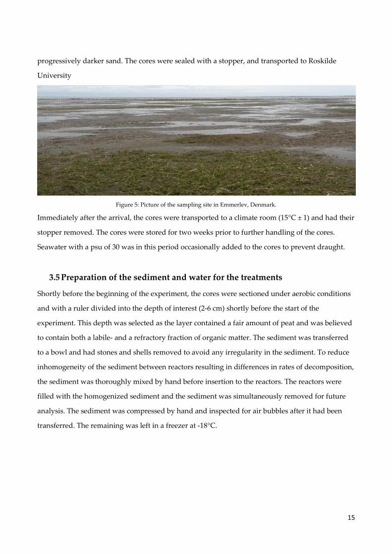
The sediment used for this study was sampled on 16 June 2015 in a salt marsh in Emmerlev,
Denmark (coordinates in degree, minutes, seconds; 54˚59'9.5''N 8˚39'24.73''E). This area lies in the
Wadden Sea and is in close vicinity to the border between Denmark and Germany. The area was
high marsh and dominated with Spartina sp. observed in patches covering the marsh (Figure 5).
The sediment was collected in cores by hand during low tide in a vegetated zone in the salt marsh.
The sampling was performed so that a Spartina sp. was present in all cores to ensure a similar
structure in all cores. The core revealed different layers in the vertical plane. The top part of the
sediment contained brown and yellow sections and was characterized with roots and other organic
material from plants. A layer of peat around three cm deep was recognizable, followed by
15
progressively darker sand. The cores were sealed with a stopper, and transported to Roskilde
University
Figure 5: Picture of the sampling site in Emmerlev, Denmark.
Immediately after the arrival, the cores were transported to a climate room (15°C ± 1) and had their
stopper removed. The cores were stored for two weeks prior to further handling of the cores.
Seawater with a psu of 30 was in this period occasionally added to the cores to prevent draught.
3.5 Preparation of the sediment and water for the treatments
Shortly before the beginning of the experiment, the cores were sectioned under aerobic conditions
and with a ruler divided into the depth of interest (2-6 cm) shortly before the start of the
experiment. This depth was selected as the layer contained a fair amount of peat and was believed
to contain both a labile- and a refractory fraction of organic matter. The sediment was transferred
to a bowl and had stones and shells removed to avoid any irregularity in the sediment. To reduce
inhomogeneity of the sediment between reactors resulting in differences in rates of decomposition,
the sediment was thoroughly mixed by hand before insertion to the reactors. The reactors were
filled with the homogenized sediment and the sediment was simultaneously removed for future
analysis. The sediment was compressed by hand and inspected for air bubbles after it had been
transferred. The remaining was left in a freezer at -18°C.
16
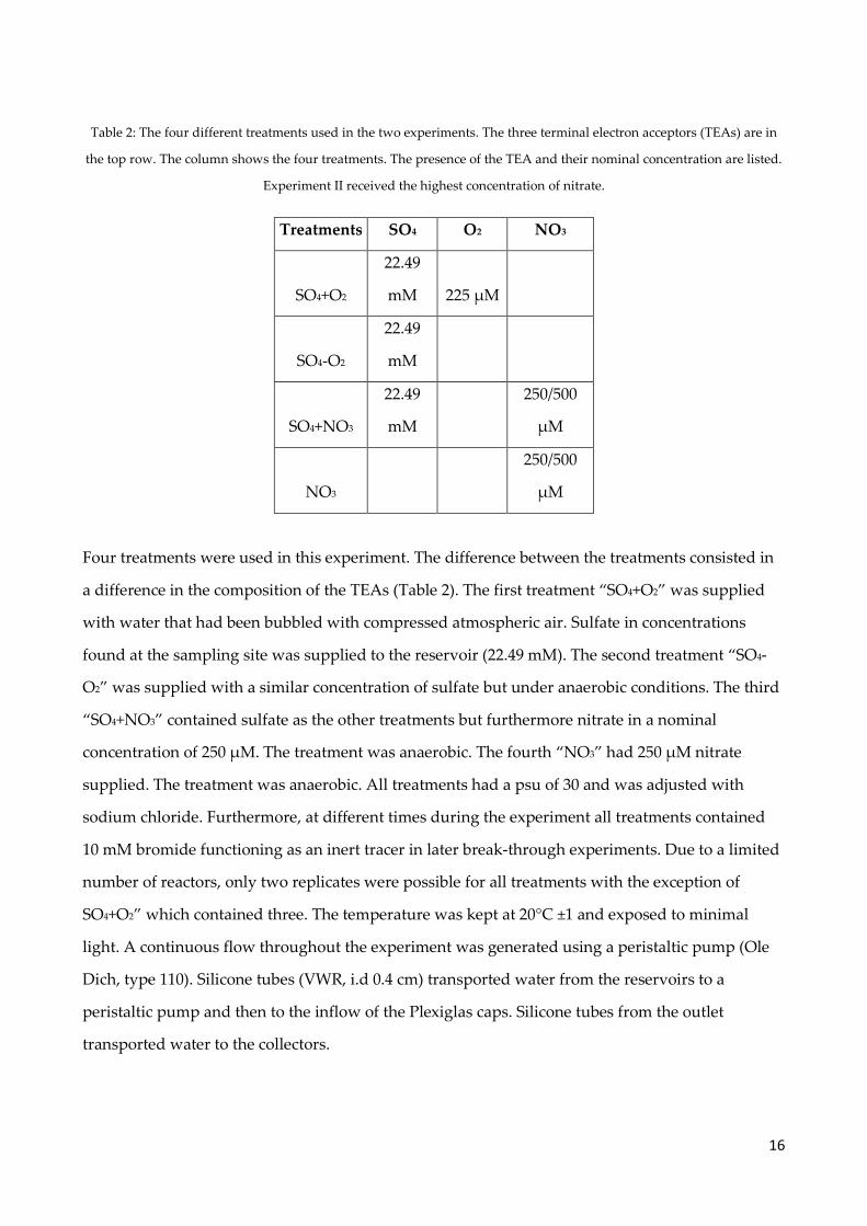
Table 2: The four different treatments used in the two experiments. The three terminal electron acceptors (TEAs) are in
the top row. The column shows the four treatments. The presence of the TEA and their nominal concentration are listed.
Experiment II received the highest concentration of nitrate.
Treatments SO4 O2 NO3
SO4+O2
22.49
mM 225 µM
SO4-O2
22.49
mM
SO4+NO3
22.49
mM
250/500
µM
NO3
250/500
µM
Four treatments were used in this experiment. The difference between the treatments consisted in
a difference in the composition of the TEAs (Table 2). The first treatment “SO4+O2” was supplied
with water that had been bubbled with compressed atmospheric air. Sulfate in concentrations
found at the sampling site was supplied to the reservoir (22.49 mM). The second treatment “SO4-
O2” was supplied with a similar concentration of sulfate but under anaerobic conditions. The third
“SO4+NO3” contained sulfate as the other treatments but furthermore nitrate in a nominal
concentration of 250 µM. The treatment was anaerobic. The fourth “NO3” had 250 µM nitrate
supplied. The treatment was anaerobic. All treatments had a psu of 30 and was adjusted with
sodium chloride. Furthermore, at different times during the experiment all treatments contained
10 mM bromide functioning as an inert tracer in later break-through experiments. Due to a limited
number of reactors, only two replicates were possible for all treatments with the exception of
SO4+O2” which contained three. The temperature was kept at 20°C ±1 and exposed to minimal
light. A continuous flow throughout the experiment was generated using a peristaltic pump (Ole
Dich, type 110). Silicone tubes (VWR, i.d 0.4 cm) transported water from the reservoirs to a
peristaltic pump and then to the inflow of the Plexiglas caps. Silicone tubes from the outlet
transported water to the collectors.
17
After termination of the experiment analysis of the samples revealed changeup had occurred for
several of the tubes. Furthermore, the analysis of the nitrate samples indicated the nitrate level was
insufficient as some of the nitrate samples were almost exhausted (confer Figure 19). Lastly, the
measurement of oxygen indicated no consumption had occurred, which seem improbable (see
Figure 21). Because of the severity of these discoveries, it was chosen to redo the experiment with
several adjustments. This experiment is referred to as experiment II later in the study, whilst the
first experiment will be referred to as experiment I. The sediment used for experiment II was the
sediment that was stored in the freezer for two months. The number of replicates was increased to
three for all treatments. The nitrate concentration was increased to 500 µM to avoid exhaustion of
nitrate. The flow rate was also increased to 50 µL/min. Spot checks of nitrate from the first days of
experiment II were performed to evaluate the level of nitrate. These samples were determined to
contain low concentrations of nitrate and consequently, the flow rate was increased to 100 µL/min
at the sixth day of the experiment. To improve the measurements of oxygen for the aerobic
treatment, less gas permeable Viton tubes (Saint-Gobain, Iso-versinic, i.d 0.4 cm) were inserted
between the reactor and the collector for the treatments “SO4+O2”.
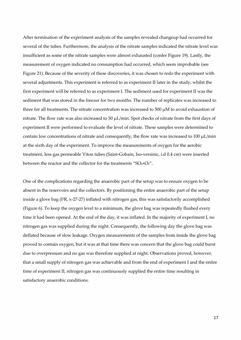
One of the complications regarding the anaerobic part of the setup was to ensure oxygen to be
absent in the reservoirs and the collectors. By positioning the entire anaerobic part of the setup
inside a glove bag (I2R, x-27-27) inflated with nitrogen gas, this was satisfactorily accomplished
(Figure 6). To keep the oxygen level to a minimum, the glove bag was repeatedly flushed every
time it had been opened. At the end of the day, it was inflated. In the majority of experiment I, no
nitrogen gas was supplied during the night. Consequently, the following day the glove bag was
deflated because of slow leakage. Oxygen measurements of the samples from inside the glove bag
proved to contain oxygen, but it was at that time there was concern that the glove bag could burst
due to overpressure and no gas was therefore supplied at night. Observations proved, however,
that a small supply of nitrogen gas was achievable and from the end of experiment I and the entire
time of experiment II, nitrogen gas was continuously supplied the entire time resulting in
satisfactory anaerobic conditions.
18
.
Figure 6: The anaerobic part of the experiment. The discs can be seen on the left side of the picture inside the glove bag.
In the middle, the peristaltic pump is found and in front of the pump, the reservoirs are located.
The collectors used for the outflow had low volumes in order to generate an overflow of the
outflow water in the collectors. This was to diminish the risk of gas-exchange. The reasoning was
that the outlet water, which had been in contact with the air, would be the first to leave the
solution if the flask experienced an overflow. The remaining water would then have experienced
minimum contact with oxygen before sampling. This was especially important in the aerobic
treatment since the sample collector flask was directly in contact with atmospheric air, and oxygen
diffusing into the collectors would lead to an underestimation of the consumption of oxygen.
To evaluate the concentration of oxygen in the water, an oxygen micro electrode connected to a
picoammeter was used every time the outflow was collected. This electrode was calibrated daily
with 30 psu water flushed with nitrogen for a measurement of 0% oxygen and flushed with
atmospheric air for a measurement of 100% oxygen. When the sampling had to be performed, the
air content for both the outflow and the reservoirs were measured. The oxygen saturation under
these circumstances was set to 225 µM based on the temperature of 20 ˚C. The outflow was after
measurement of the oxygen content transferred to a 10 mL glass exetainer (LABOCO LTD) and
either 15 or 50 mL plastic centrifuge tubes (Nunc). The exetainer was stored in a refrigerator (5°C)
and the tubes were kept in a freezer (-18°C) until analysis. After termination of the experiment, the
19
reactors were opened and inspected. Sediments were sampled as they had been during the reactor
preparation.
3.6 Analysis of samples
The concentration of different TEA’s used in this experiment, (nitrate, sulfate, and oxygen) were
analyzed. Furthermore, carbon dioxide was used as a benchmark to comparison of these. The FTR
experimental setup allowed a calculation of the consumption/production of the listed compounds.
The flow and supply of reactant is in a FTR experiment supplied at a constant pace resulting in a
steady state, at which the consumption of different terminal electron acceptors (TEA) can be
calculated by the use of (Eq. 7) found in Pallud et al. (2007). R denotes consumption, Cin the
concentration of the solution supplied to the reactors, whilst Cout is the measured solution after it
has been in the reactor. Q is the flow rate and V is the volume. This equation was used to calculate
the kinetics of oxygen, sulfate, nitrate, and carbon dioxide. An example of a calculation of this can
be found in the appendix.
7 = (89: − 8<=>) ∗ ?
@ (Eq. 7)
At various times, especially for experiment I, the TEA in the reservoirs reservoirs were not
frequently measured and in these situations the average value of other reservoirs measurements
were used. Once, in each of the two experiments a break through curve was performed using
bromide as a tracer. This was performed using the method described in Presley (1971) where
bromide is added to the reservoir to a concentration of 10 µM and the bromide concentration in the
outflow is measured over time. Bromide was additionally measured on the IC and was used to
correct sulfate measurements for experiment II. A refractometer (ATAGO S/MII) measured the
salinity. Sediment properties bulk and elemental composition were also investigated for each
experiment. These includes porosity, dry density, loss on ignition (LOI; muffle oven, VECSTAR),
CHN analyzed (Elemental Analyzer, FLASH 2000). Carbon dioxide was measured through the
new GSIRe method, which was optimized and compared beforehand of the sampling in the
experiments (confer 4.2). Nitrate was measured by a Lachat flow Injection analyser (Quick Chem
FIA+, 8000 series). The lowest standard measured was 0.5 µM. Sulfate was measured by the use of
20
an ion chromatograph (IC, Dionex, ICS-1100). Sulfate was furthermore measured by the new fAAS
method (see section 3.2). The concentration of dissolved oxygen was measured by a microelectrode
(Unisense, OX-500) connected to a picoammeter, (Unisense, PA2000). It was calibrated by bubbling
atmospheric air inside it for five min and then measured. The water was then bubbled with
atmospheric nitrogen for five min and then measured. These corresponds to readings of 0 and 100
% oxygen saturation. This calibration was not always performed for experiment I and for the
missing data, an average of the remaining have been used. For the entire experiment II experiment,
the electrode was calibrated correctly for all days. A combined pH electrode (Radiometer, pHC
2015-8) connected to a standard pH meter (Radiometer, PHM210) measured pH during
experiment II. A list of the chemicals and materials used are located in the appendix
3.7 Statistical analysis
The data obtained from the analysis of samples from the two experiments was statistically
analyzed using the statistic program “Systat” (version 13). The α-value was set to 0.05 for all
instances. The daily carbon dioxide rate and cumulative production were analyzed using either the
parametric (ANOVA) or the non-parametric test (Kruskal-Wallis) for selected times during the
experiment. If one sample did not have similar variance and normal distribution at the selected
day, the samples were analyzed using Kruskal-Wallis. For the entire thesis, when no other
information is listed, the ± symbol represents 1 standard error of the mean (SEM).
4. Results
4.1 Evaluation of the fAAS method
The fAAS method for sulfate measurements was assessed to complement if not replace the IC for
measurements of sulfate in marine waters. To evaluate the accuracy and precision of the method a
calibration curve of different sulfate concentrations ranging from 0 mM to 28 mM was performed.
2 mL 36.58 mM barium, 1 mL of 0.5 M HCl and different volumes of a sulfate stock solution (28
mM) was prepared in order to make sulfate concentrations of 0, 7, 14, 21 and 28 mM SO���. To
diminish the potential interference from carbonate and to investigate the importance of it, three
samples supplied with 21 mM SO��� (21 mM water) were not acidified but instead deionized water
21
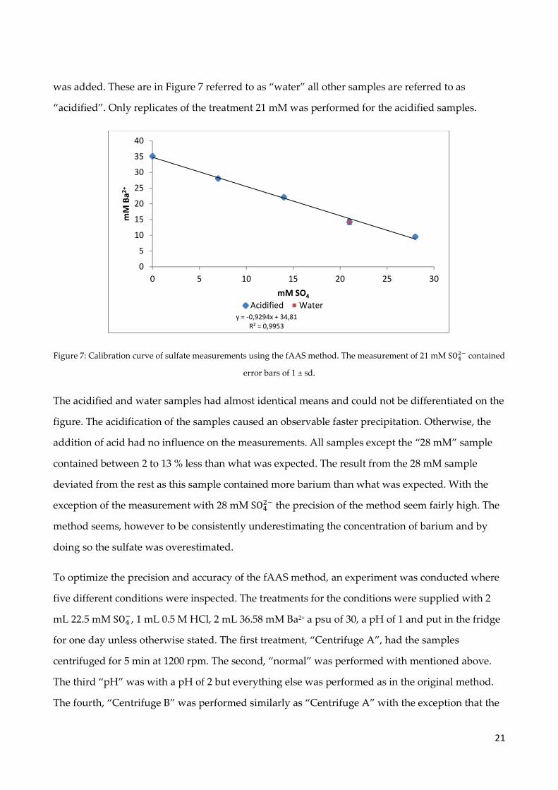
was added. These are in Figure 7 referred to as “water” all other samples are referred to as
“acidified”. Only replicates of the treatment 21 mM was performed for the acidified samples.
Figure 7: Calibration curve of sulfate measurements using the fAAS method. The measurement of 21 mM SO��� contained
error bars of 1 ± sd.
The acidified and water samples had almost identical means and could not be differentiated on the
figure. The acidification of the samples caused an observable faster precipitation. Otherwise, the
addition of acid had no influence on the measurements. All samples except the “28 mM” sample
contained between 2 to 13 % less than what was expected. The result from the 28 mM sample
deviated from the rest as this sample contained more barium than what was expected. With the
exception of the measurement with 28 mM SO��� the precision of the method seem fairly high. The
method seems, however to be consistently underestimating the concentration of barium and by
doing so the sulfate was overestimated.
To optimize the precision and accuracy of the fAAS method, an experiment was conducted where
five different conditions were inspected. The treatments for the conditions were supplied with 2
mL 22.5 mM SO��, 1 mL 0.5 M HCl, 2 mL 36.58 mM Ba2+ a psu of 30, a pH of 1 and put in the fridge
for one day unless otherwise stated. The first treatment, “Centrifuge A”, had the samples
centrifuged for 5 min at 1200 rpm. The second, “normal” was performed with mentioned above.
The third “pH” was with a pH of 2 but everything else was performed as in the original method.
The fourth, “Centrifuge B” was performed similarly as “Centrifuge A” with the exception that the
y = -0,9294x + 34,81
R² = 0,9953
0
5
10
15
20
25
30
35
40
0 5 10 15 20 25 30
mM
Ba
2+
mM SO4
Acidified Water
22
sample was not cooled but instead analyzed within 2 hours. To inspect the reproducibility of the
measurements, one of the replicates from the treatment “Centrifuge A” was analyzed thrice. This
treatment is referred to as “Reproducibility”.
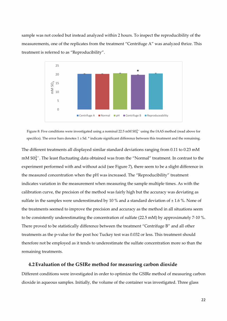
Figure 8: Five conditions were investigated using a nominal 22.5 mM SO��� using the fAAS method (read above for
specifics). The error bars denotes 1 ± Sd. * indicate significant difference between this treatment and the remaining.
The different treatments all displayed similar standard deviations ranging from 0.11 to 0.23 mM
mM SO���. The least fluctuating data obtained was from the “Normal” treatment. In contrast to the
experiment performed with and without acid (see Figure 7), there seem to be a slight difference in
the measured concentration when the pH was increased. The “Reproducibility” treatment
indicates variation in the measurement when measuring the sample multiple times. As with the
calibration curve, the precision of the method was fairly high but the accuracy was deviating as
sulfate in the samples were underestimated by 10 % and a standard deviation of ± 1.6 %. None of
the treatments seemed to improve the precision and accuracy as the method in all situations seem
to be consistently underestimating the concentration of sulfate (22.5 mM) by approximately 7-10 %.
There proved to be statistically difference between the treatment “Centrifuge B” and all other
treatments as the p-value for the post hoc Tuckey test was 0.032 or less. This treatment should
therefore not be employed as it tends to underestimate the sulfate concentration more so than the
remaining treatments.
4.2 Evaluation of the GSIRe method for measuring carbon dioxide
Different conditions were investigated in order to optimize the GSIRe method of measuring carbon
dioxide in aqueous samples. Initially, the volume of the container was investigated. Three glass
0
5
10
15
20
25
mM
SO
4
Centrifuge A Normal pH Centrifuge B Reproduceability
*
23
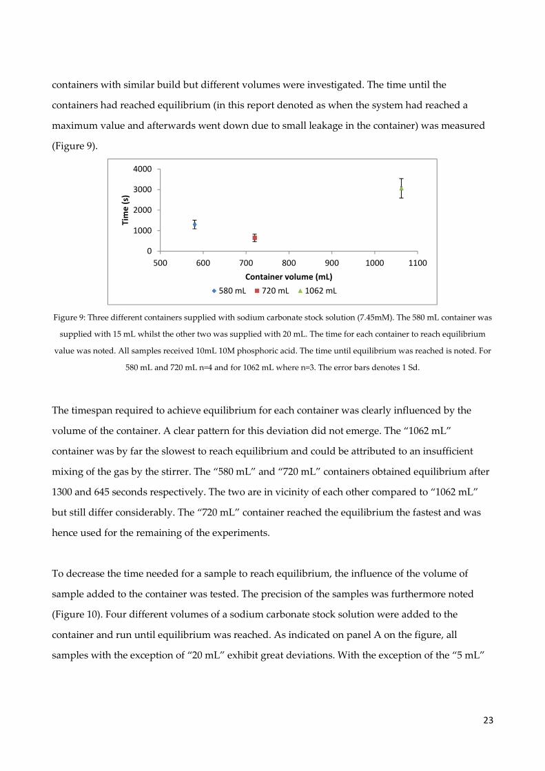
containers with similar build but different volumes were investigated. The time until the
containers had reached equilibrium (in this report denoted as when the system had reached a
maximum value and afterwards went down due to small leakage in the container) was measured
(Figure 9).
Figure 9: Three different containers supplied with sodium carbonate stock solution (7.45mM). The 580 mL container was
supplied with 15 mL whilst the other two was supplied with 20 mL. The time for each container to reach equilibrium
value was noted. All samples received 10mL 10M phosphoric acid. The time until equilibrium was reached is noted. For
580 mL and 720 mL n=4 and for 1062 mL where n=3. The error bars denotes 1 Sd.
The timespan required to achieve equilibrium for each container was clearly influenced by the
volume of the container. A clear pattern for this deviation did not emerge. The “1062 mL”
container was by far the slowest to reach equilibrium and could be attributed to an insufficient
mixing of the gas by the stirrer. The “580 mL” and “720 mL” containers obtained equilibrium after
1300 and 645 seconds respectively. The two are in vicinity of each other compared to “1062 mL”
but still differ considerably. The “720 mL” container reached the equilibrium the fastest and was
hence used for the remaining of the experiments.
To decrease the time needed for a sample to reach equilibrium, the influence of the volume of
sample added to the container was tested. The precision of the samples was furthermore noted
(Figure 10). Four different volumes of a sodium carbonate stock solution were added to the
container and run until equilibrium was reached. As indicated on panel A on the figure, all
samples with the exception of “20 mL” exhibit great deviations. With the exception of the “5 mL”
0
1000
2000
3000
4000
500 600 700 800 900 1000 1100
Tim
e (
s)
Container volume (mL)
580 mL 720 mL 1062 mL
24
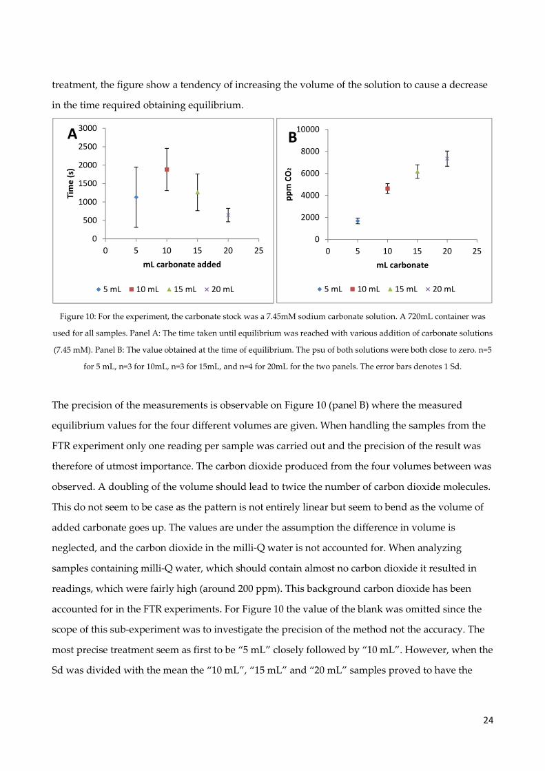
treatment, the figure show a tendency of increasing the volume of the solution to cause a decrease
in the time required obtaining equilibrium.
Figure 10: For the experiment, the carbonate stock was a 7.45mM sodium carbonate solution. A 720mL container was
used for all samples. Panel A: The time taken until equilibrium was reached with various addition of carbonate solutions
(7.45 mM). Panel B: The value obtained at the time of equilibrium. The psu of both solutions were both close to zero. n=5
for 5 mL, n=3 for 10mL, n=3 for 15mL, and n=4 for 20mL for the two panels. The error bars denotes 1 Sd.
The precision of the measurements is observable on Figure 10 (panel B) where the measured
equilibrium values for the four different volumes are given. When handling the samples from the
FTR experiment only one reading per sample was carried out and the precision of the result was
therefore of utmost importance. The carbon dioxide produced from the four volumes between was
observed. A doubling of the volume should lead to twice the number of carbon dioxide molecules.
This do not seem to be case as the pattern is not entirely linear but seem to bend as the volume of
added carbonate goes up. The values are under the assumption the difference in volume is
neglected, and the carbon dioxide in the milli-Q water is not accounted for. When analyzing
samples containing milli-Q water, which should contain almost no carbon dioxide it resulted in
readings, which were fairly high (around 200 ppm). This background carbon dioxide has been
accounted for in the FTR experiments. For Figure 10 the value of the blank was omitted since the
scope of this sub-experiment was to investigate the precision of the method not the accuracy. The
most precise treatment seem as first to be “5 mL” closely followed by “10 mL”. However, when the
Sd was divided with the mean the “10 mL”, “15 mL” and “20 mL” samples proved to have the
0
500
1000
1500
2000
2500
3000
0 5 10 15 20 25
Tim
e (
s)
mL carbonate added
5 mL 10 mL 15 mL 20 mL
A
0
2000
4000
6000
8000
10000
0 5 10 15 20 25
pp
m C
O2
mL carbonate
B
5 mL 10 mL 15 mL 20 mL

25
lowest deviation based on percentage. Consequentially, it was chosen to use 10 mL for the
experiment based on its high precision.
The time required for the system to reach equilibrium, the accuracy and the precision of the
method were unacceptable if numerous samples had to be analyzed. To decrease the time to reach
equilibrium, different conditions were investigated. The first of these was to inspect the influence
in the molarity of the acid added to the sample. Phosphoric acid with concentrations of 1M or 15M
were added to a 7.45 mM concentration of a sodium carbonate solution (Figure 11). Each
phosphoric acid molecule could potentially dissociates three protons. The pKa for phosphoric acid
are 2.12, 7.21, and 12.319 (Chang 2008). The pH of the solution would be less than pH 1 even with
1M phosphoric acid. For a solution of 1mM carbonate and 1M phosphoric acid, the number of
oxonium ions per dissolved carbon dioxide molecules would be close to 3,000:1 whilst for 15 M it
will be 45,000.
Figure 11: The graph show the development of carbon dioxide where 20mL 7.45mM sodium carbonate stock solution
and 10mL 1M or 15M phosphoric acid was added to a solution. Three replicas for respectively 1M and 15M are noted on
the figure.
The development of carbon dioxide was similar and the difference in the result by using 1 or 15M
acid does not seem to influence the time and the measured value. To avoid unnecessary risk by
handling high molarity acid 1 M phosphoric acid was selected for the remaining experiments.
0
1000
2000
3000
4000
5000
6000
7000
0 200 400 600 800 1000 1200 1400 1600 1800
pp
m C
O2
Time (s)
1 M replica 1 1 M replica 2 1 M replica 3
15 M Replica 1 15 M Replica 2 15 M Replica 3

26
Another initiative to decrease the time required per sample was by increasing the temperature of
the added acid thereby increasing the reaction rate. This was tested by heating 1M phosphoric acid
to 70°C and compare it to one performed at room temperature (Figure 12). The sodium carbonate
solution was not heated but was instead room temperature.
Figure 12: The figure shows two different temperatures (listed in ˚C) of phosphoric acid (20 and 70 ˚C) and 20mL 9.45
mM sodium carbonate solutions. n=1 in both instances.
The development for the two treatments was over the entire period almost identical and the
temperature did not at these temperatures influence the rate of the reaction. It was chosen to
operate with acid at room temperature to avoid handling with hot phosphoric acid.
After performing this experiment, it was observed that after approximately 350 seconds, the
system approached equilibrium. This pattern was also evident from the readings used for Figure
10. It was chosen to perform an experiment with replicas of 10 mL 7.45 mM sodium carbonate to
see if the development was stable (Figure 13). The development for all replicas display a steep
increase during the initial 200 second followed by a flattening for the remaining period. This
development was also evident in other scenarios such as in Figure 12.
0
500
1000
1500
2000
2500
3000
3500
4000
4500
0 200 400 600 800 1000
pp
m C
O2
Time (s)
20 degrees 70 degrees

27
Figure 13: The figure shows the run of three replicates with 10mL 7.45 mM CO32- and 10 mL 10 M H3PO4 of an analysis
run on the customized carbon dioxide analyser.
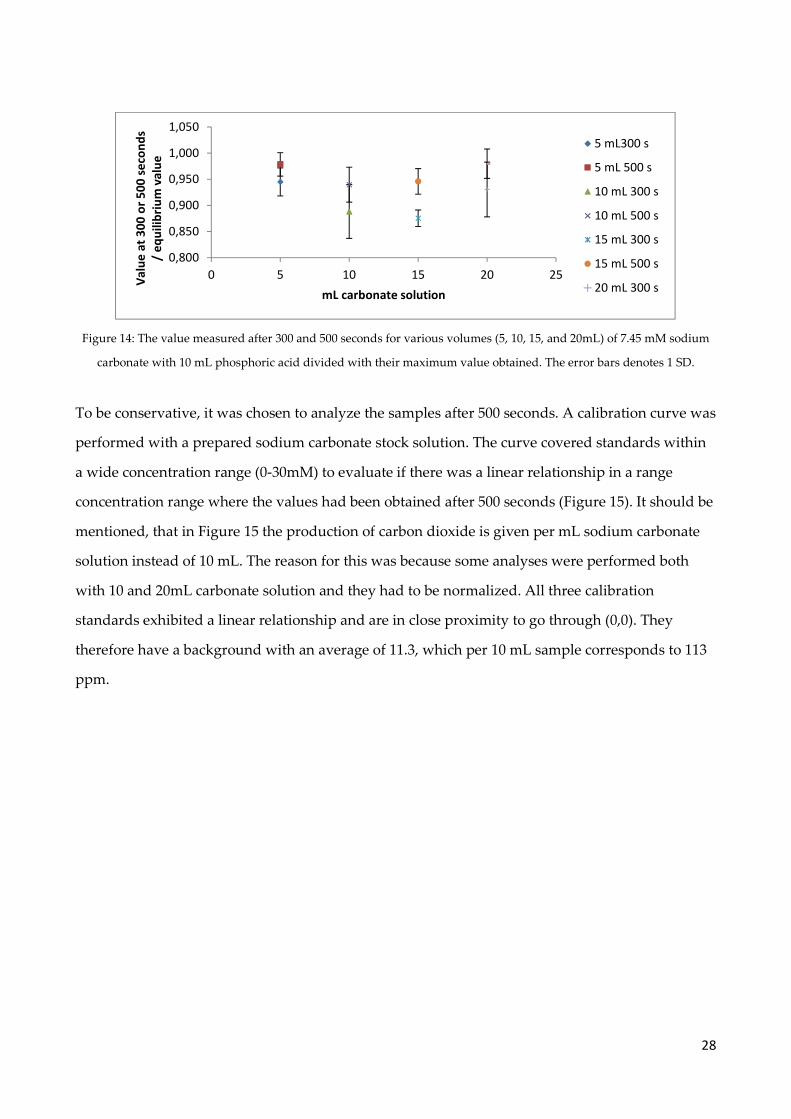
To inspect if it was possible to decrease the time for each sample, the equilibrium values from
Figure 10 was divided with the value of carbon dioxide measured after 300 and 500 seconds and
compared (Figure 14). The values taken after 500 seconds was closer to the equilibrium values,
compared to those registered after 300 seconds. The minor difference in the measured carbon
dioxide value for all scenarios between registering the carbon dioxide value after 500 seconds or at
the equilibrium (Figure 10) made it seem plausible to get stable values by noting the value after
500 seconds. The reason why a reading after 300 seconds was not in consideration despite it being
able to produce faster measurements was because it was feared the samples might not all reach the
stable plateau. The samples would possibly not have had enough time to get close to the
equilibrium value, which would have led to an underestimation of the carbon dioxide level in the
water sample.
0
1000
2000
3000
4000
5000
6000
0 500 1000 1500 2000 2500 3000 3500
pp
m C
O2
Time (s)
28
Figure 14: The value measured after 300 and 500 seconds for various volumes (5, 10, 15, and 20mL) of 7.45 mM sodium
carbonate with 10 mL phosphoric acid divided with their maximum value obtained. The error bars denotes 1 SD.
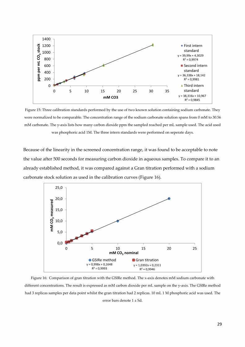
To be conservative, it was chosen to analyze the samples after 500 seconds. A calibration curve was
performed with a prepared sodium carbonate stock solution. The curve covered standards within
a wide concentration range (0-30mM) to evaluate if there was a linear relationship in a range
concentration range where the values had been obtained after 500 seconds (Figure 15). It should be
mentioned, that in Figure 15 the production of carbon dioxide is given per mL sodium carbonate
solution instead of 10 mL. The reason for this was because some analyses were performed both
with 10 and 20mL carbonate solution and they had to be normalized. All three calibration
standards exhibited a linear relationship and are in close proximity to go through (0,0). They
therefore have a background with an average of 11.3, which per 10 mL sample corresponds to 113
ppm.
0,800
0,850
0,900
0,950
1,000
1,050
0 5 10 15 20 25
Va
lue
at
30
0 o
r 5
00
se
con
ds
/ e
qu
ilib
riu
m v
alu
e
mL carbonate solution
5 mL300 s
5 mL 500 s
10 mL 300 s
10 mL 500 s
15 mL 300 s
15 mL 500 s
20 mL 300 s
29
Figure 15: Three calibration standards performed by the use of two known solution containing sodium carbonate. They
were normalized to be comparable. The concentration range of the sodium carbonate solution spans from 0 mM to 30.56
mM carbonate. The y-axis lists how many carbon dioxide ppm the sampled reached per mL sample used. The acid used
was phosphoric acid 1M. The three intern standards were performed on seperate days.
Because of the linearity in the screened concentration range, it was found to be acceptable to note
the value after 500 seconds for measuring carbon dioxide in aqueous samples. To compare it to an
already established method, it was compared against a Gran titration performed with a sodium
carbonate stock solution as used in the calibration curves (Figure 16).
Figure 16: Comparison of gran titration with the GSIRe method. The x-axis denotes mM sodium carbonate with
different concentrations. The result is expressed as mM carbon dioxide per mL sample on the y-axis. The GSIRe method
had 3 replicas samples per data point whilst the gran titration had 2 replicas. 10 mL 1 M phosphoric acid was used. The
error bars denote 1 ± Sd.
y = 38,316x + 10,967
R² = 0,9845
y = 36,338x + 18,142
R² = 0,9981
y = 39,99x + 4,3029
R² = 0,9974
0
200
400
600
800
1000
1200
1400
0 5 10 15 20 25 30 35
pp
m p
er
mL
CO
3st
ock
mM CO3
First intern
standard
Second intern
standard
Third intern
standard
y = 0,998x + 0,1648
R² = 0,9993y = 1,0392x + 0,2311
R² = 0,9946
0,0
5,0
10,0
15,0
20,0
25,0
0 5 10 15 20 25
mM
CO
3m
ea
sure
d
mM CO3 nominal
GSIRe method Gran titration

30
The calibration curve used for this figure was conducted the same day as the Gran titration was
performed. The two methods agreed well on the concentration of solutions containing sodium
carbonate in the investigated range. The GSIRe method was with this verified to be capable of
measuring samples in the range of 0mM to 5mM carbonate in aqueous samples, which were
within the range measured in the flow through experiment.
4.3 Sediment properties
To evaluate if the sediment was homogenized and to evaluate any possible change that occurred
during the experiment, the sediment was qualitatively and quantitatively analyzed before and
after both experiments (Table 3). At all times in both experiments, no sulfide-odor but rather an
organic smell was detectable from the sediment. After each experiment, the reactors were opened
and investigated for different shades and coloring around and inside the reactors. Dark spots and
light gray spots were present in and around the reactors. For both experiment I and II, the reactors
displayed the two to various degrees. The spots were useful in identification of hydraulic “dead
spots” where the water had less than optimal water circulation. After inspection (see below), the
sediment was homogenized and analyzed.
For experiment I, the outside of the sediment in the “SO4+O2” treatment were found to contain
gray areas but the majority of the sediment was dark. Inside the reactor, a gray layer was present
in the first 3 to 5 mm measured from the inlet and subsequently becoming darker. The “SO4 –O2”
treatment was almost entirely dark. As the sediment was sectioned, it proved to be entirely dark.
The “SO4+NO3” treatment proved to be almost completely dark around the sides. The inlet of both
was gray but changed to dark in 1 mm. The sediment of the treatment “NO3” was mainly dark
around the sides.
For experiment II, the sediment from the “SO4+O2” treatment were characterized by a light gray
colour around the sides of the reactor. Dark spots covered from 10 to 30% of the reactors. When
sectioned, the reactor displayed both gray and dark areas. The majority of the sediment was gray,
especially at the inlet and then turned darker at the outlet. The treatment “SO4–O2” was
characterized by an extremely thin surface of gray area at the inlet. This layer was for all three
reactors 1 mm thin or less, whilst dark sediment covered the remaining areas. The dark spots of
31
the side of the reactors covered an area of 60 to 90% of the side of the sediment. The treatment
“SO4+NO3” displayed black and light-gray areas. They were darker than the “SO4+O2” treatment
but lighter than the “SO4–O2”. The sides covered 30 to 80% of the sediment and exhibited a patchy
pattern of dark spots. The front of the reactors were all gray, but the colour shifted to dark within
1-2 mm. The treatment “NO3” exhibited darker parts than the aerobic sulfate treatment but
otherwise was quite light gray. The dark spots that were present in the sides were evenly
distributed and covered from 40 to 60% of the reactors. When the reactors were opened, they
contained a 2 to 3 mm light area and subsequently getting darker.
The procedure in analyzing and handling the sediment was identical for the two experiments,
except for one major difference. The sediment used for experiment II was the remaining part of the
depth of interest part from experiment I. This sediment had been frozen for 2 months at -18˚C prior
to the experiment. After the experiment was performed the sediment from the reactors were
analyzed. These two fractions are classified as “start sediment” and “end sediment” followed by
the number of the experiment in the table below. The samples were dried at 105 ˚C for 24 hours to
calculate dry bulk density and porosity. The organic matter content was measured by loss on
ignition (LOI) after 2 hours of 550˚C of the dried sediment by a muffle furnace. The weight
percentage of the carbon and nitrogen organic was analyzed on a CHN analyzer. These values and
other essential properties are listed in Table 3.

32
Table 3: Sediment properties for the two experiment. The samples were analyzed before and after the experiment for
comparison. The C:N ratio is listed in moles. The values are average ± SEM.
LOI %
Porosity
(%)
Dry bulk
density g cm-3
C organic
(wt%)
Organic N
(wt%)
Molar C:N
ratio
Start sediment for
experiment I
2.62 ±
0.32
49.6 ±
0.684 1.157 ± 0.019 1.307 ± 0.17
0.085 ±
0.020
19.89 ±
3.07
End of experiment I
1.95 ±
0.14
41.2 ±
0.50 1.304 ± 0.017
0.867 ±
0.030
0.053 ±
0.0007
19.05 ±
0.52
Start sediment for
experiment II
2.35 ±
0.38
42.5 ±
3.2 1.17 ± 0.029 1.07 ± 0.067
0.121 ±
0.021
12.27 ±
2.49
End of experiment II
2.69 ±
0.11
39.6 ±
0.6 1.348 ± 0.011
1.022 ±
0.036
0.070 ±
0.001
16.98 ±
0.58
The sediment used in the two experiments had, both before and after the experiments, similar
characteristics with overlapping standard error of the means for several of the measured
properties (see Table 3). The organic matter was stable for all four measurements ranging from 1.95
to 2.69% and did not systematically change during the course of the experiment. The dry bulk
density for the sediment measured before insertion in the reactors was 1.16 g cm-3 whilst it for the
sediment after was 1.33 g cm-3. The sediment being less compressed before insertion into the
reactors possibly caused this difference.
4.4 Bromide experiment
The flow rate was measured on several days for both experiments. The average measured flow
rate for experiment I was 2.08 ± 0.1 mL/h where 3 mL was expected based on pump settings. For
experiment II, the measured flow rate was 5.29 ± 0.12 mL/h and the expected was 6 mL/h. To
evaluate and check for non-ideal flow conditions of the fluid inside the reactors, bromide was used
as a tracer and measured once during both experiments, by the method used in (Presley 1971). The
time at which this was executed was 6 weeks for experiment I and 3 weeks for experiment II.
Reservoirs were supplied with the water (with and without bromide for experiment I and II, see
below) and the tubes were flushed. The tubes were afterwards attached to the inlet and the

33
experiment was started. This equals time 0 denoted in Figure 17 and Figure 18. The outlet was
collected at different intervals until the water from the outlet was identical to the water from the
reservoirs. The measured values were normalized to the value of the reservoirs by dividing the
measured value (C0) with the concentration in the reservoirs (C). The number following each
treatment denote the number of replica.
For experiment I, only eight out of nine reactors were available. The missing reactor was the
“SO4+NO3 1” which leaked during the experiment and therefore was omitted from the experiment.
The reactors were supplied with water containing 10 mM bromide and their normal electron
acceptor composition. All reactors display a similar sigmoidal pattern in breakthrough time. All
contained bromide in the same concentrations as the reservoirs after approximately 23 hours.
Roychoudhury et al. (1998) used bromide as an inert tracer to inspect the flow conditions in the
reactor. This was done in order to see if the calculated break through was similar to the measured.
If the calculated and the measured break through disagrees it point towards irregular flow inside
the reactor. This study used the same method, and the used calculation is observed below.
A = 8<
8=
12
BCDE(F − μH
2IJ>H) (Eq. 8)
F is the cumulative age distribution curve. The L stands is the length of the reactor, Dt is the
longitudinal dispersion coefficient, indicating how the solute behaves in the longitudinal direction,
and is a useful parameter to describe flow characteristics. t stands for time, and µ is calculated by
(Eq. 9).
μ =?
KL (Eq. 9)
erfc is the complimentary error function. Q is the experimentally measured flow rate, A is the cross
sectional area of the reactor, and ϕ is the porosity. Using the equation, it was possible to fit a graph
by changing Dt until the complimentary function was comparable to the measured values. The
calculated longitudinal dispersion coefficient obtained this way was 1.25 *10-3 cm2 s-1 which is only
a bit above the values listed in (Roychoudhury et al. 1998).
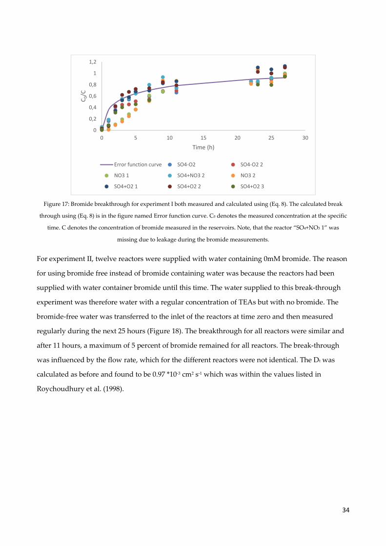
34
Figure 17: Bromide breakthrough for experiment I both measured and calculated using (Eq. 8). The calculated break
through using (Eq. 8) is in the figure named Error function curve. C0 denotes the measured concentration at the specific
time. C denotes the concentration of bromide measured in the reservoirs. Note, that the reactor “SO4+NO3 1” was
missing due to leakage during the bromide measurements.
For experiment II, twelve reactors were supplied with water containing 0mM bromide. The reason
for using bromide free instead of bromide containing water was because the reactors had been
supplied with water container bromide until this time. The water supplied to this break-through
experiment was therefore water with a regular concentration of TEAs but with no bromide. The
bromide-free water was transferred to the inlet of the reactors at time zero and then measured
regularly during the next 25 hours (Figure 18). The breakthrough for all reactors were similar and
after 11 hours, a maximum of 5 percent of bromide remained for all reactors. The break-through
was influenced by the flow rate, which for the different reactors were not identical. The Dt was
calculated as before and found to be 0.97 *10-3 cm2 s-1 which was within the values listed in
Roychoudhury et al. (1998).
0
0,2
0,4
0,6
0,8
1
1,2
0 5 10 15 20 25 30
C0/C
Time (h)
Error function curve SO4-O2 SO4-O2 2
NO3 1 SO4+NO3 2 NO3 2
SO4+O2 1 SO4+O2 2 SO4+O2 3
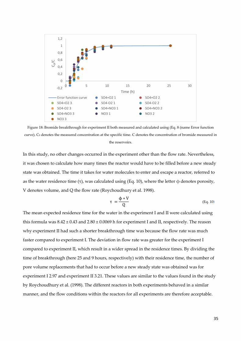
35
Figure 18: Bromide breakthrough for experiment II both measured and calculated using (Eq. 8 (name Error function
curve). C0 denotes the measured concentration at the specific time. C denotes the concentration of bromide measured in
the reservoirs.
In this study, no other changes occurred in the experiment other than the flow rate. Nevertheless,
it was chosen to calculate how many times the reactor would have to be filled before a new steady
state was obtained. The time it takes for water molecules to enter and escape a reactor, referred to
as the water residence time (τ), was calculated using (Eq. 10), where the letter ϕ denotes porosity,
V denotes volume, and Q the flow rate (Roychoudhury et al. 1998).
τ =ϕ ∗ V
Q (Eq. 10)
The mean expected residence time for the water in the experiment I and II were calculated using
this formula was 8.42 ± 0.43 and 2.80 ± 0.0069 h for experiment I and II, respectively. The reason
why experiment II had such a shorter breakthrough time was because the flow rate was much
faster compared to experiment I. The deviation in flow rate was greater for the experiment I
compared to experiment II, which result in a wider spread in the residence times. By dividing the
time of breakthrough (here 25 and 9 hours, respectively) with their residence time, the number of
pore volume replacements that had to occur before a new steady state was obtained was for
experiment I 2.97 and experiment II 3.21. These values are similar to the values found in the study
by Roychoudhury et al. (1998). The different reactors in both experiments behaved in a similar
manner, and the flow conditions within the reactors for all experiments are therefore acceptable.
-0,2
0
0,2
0,4
0,6
0,8
1
1,2
0 5 10 15 20 25 30
C0/C
Time (h)
Error function curve SO4+O2 1 SO4+O2 2
SO4+O2 3 SO4-O2 1 SO4-O2 2
SO4-O2 3 SO4+NO3 1 SO4+NO3 2
SO4+NO3 3 NO3 1 NO3 2
NO3 3
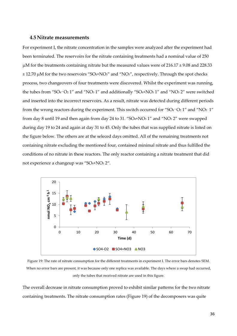
36
4.5 Nitrate measurements
For experiment I, the nitrate concentration in the samples were analyzed after the experiment had
been terminated. The reservoirs for the nitrate containing treatments had a nominal value of 250
µM for the treatments containing nitrate but the measured values were of 216.17 ± 9.08 and 228.33
± 12.70 µM for the two reservoirs “SO4+NO3” and “NO3”, respectively. Through the spot checks
process, two changeovers of four treatments were discovered. Whilst the experiment was running,
the tubes from “SO4—O2 1” and “NO3 1” and additionally “SO4+NO3 1” and “NO3 2” were switched
and inserted into the incorrect reservoirs. As a result, nitrate was detected during different periods
from the wrong reactors during the experiment. This switch occurred for “SO4—O2 1” and “NO3 1”
from day 8 until 19 and then again from day 24 to 31. “SO4+NO3 1” and “NO3 2” were swapped
during day 19 to 24 and again at day 31 to 45. Only the tubes that was supplied nitrate is listed on
the figure below. The others are at the seleced days omitted. All of the remaining treatments not
containing nitrate excluding the mentioned four, contained minimal nitrate and thus fulfilled the
conditions of no nitrate in these reactors. The only reactor containing a nitrate treatment that did
not experience a changeup was “SO4+NO3 2“.
Figure 19: The rate of nitrate consumption for the different treatments in experiment I. The error bars denotes SEM.
When no error bars are present, it was because only one replica was available. The days where a swap had occurred,
only the tubes that received nitrate are used in this figure.
The overall decrease in nitrate consumption proved to exhibit similar patterns for the two nitrate
containing treatments. The nitrate consumption rates (Figure 19) of the decomposers was quite
0
5
10
15
20
0 10 20 30 40 50 60 70
nm
ol
NO
3cm
-3h
.1
Time (d)
SO4-O2 SO4+NO3 NO3

37
stable for all treatments during the entire experiment, including the ones that were swapped. In
the initial days of the experiment, the consumption rates may have been underestimated as the
outlets contained low concentrations of nitrate and were close to completely depletion in the
outlets.
For experiment II, the nitrate concentration was increased to 500 µM to minimize the potential risk
of nitrate depletion as was observed in experiment I. This increase proved to be insufficient, as the
consumption approached values close to those of the reservoirs in the start of the experiment as
“SO4+NO3” and “NO3” consumed 421.55 ± 10.00 and 441.45 ± 13.82 µM during the first six days of
the experiment. To avoid exhaustion of nitrate, the flow rate was increased from 50 µL/min to 100
µL/min on the sixth day of the experiments. This decreased the measured nitrate value in the
outlets but the overall nitrate consumption remained unchanged (Figure 20). The increased flow
rate and nitrate concentration enabled a surplus of nitrate for the remaining of the experiment.
Figure 20: The nitrate consumption rates for experiment II from the two nitrate treatments. The line display where the
flow rate was changed. Data is shown as mean ± SEM.
4.6 Oxygen measurements
The oxygen consumption was, as mentioned in the method section calculated based on
measurements from a micro electrode. In experiment I, the samples inside the glove bag contained
low levels of oxygen (12.3 ± 0.96%) for the anaerobic treatments. Satisfactory anaerobic conditions
were first obtained when nitrogen was continuously supplied into the glove bag.
0
5
10
15
20
25
30
35
40
45
0 5 10 15 20 25 30 35 40
nm
ol
NO
3cm
-3h
-1
Time (d)
SO4+NO3 NO3

38
Figure 21: The oxygen consumption rate for the two experiments listed in nmol cm-3 h-1. “SO4+O2 1” indicate experiment
I, and “SO4+O2 2” experiment II. The line denotes where the flow rate was changed for experiment II. The error bars are
SEM. All data points have error bars.
The measured oxygen consumption rate was lower for experiment I compared to experiment II
(Figure 21). Almost no oxygen consumption was evident in the experiment I and the consumption
rate reached a maximum and minimum of 4.03 and -1.07 nmol cm-3 h-1, respectively, whilst it for
experiment II was between 23.14 and 0.48 nmol cm-3 h-1. The mean for experiment I was 0.53 ± 0.27
nmol cm-3 h-1. For experiment II, the mean consumption rate for the entire experiment was 13.39 ±
0.88 nmol cm-3 h-1. The mean after the flow rate was changed it was 15.76 ± 0.78 nmol cm-3 h-1.
4.7 Sulfate measurements
Experiment I exhibited numerous complications and the measurement of sulfate proved to be one
of these. As mentioned in the nitrate result section (4.5) there had been numerous changeups of the
tubes during experiment I. These changeups were identified through sulfate measurement by
samples from the treatment “NO3” which detected a presence of sulfate. The data for the days
where the tubes have been swapped were not included in the figure below. “NO3” was therefore
omitted from the figure despite it containing sulfate at various times throughout the experiment.
The measurement from the other (not switched) replicate of the reactor was used when possible.
Because of this, not all the data points contained error bars, as there was only one measurement
available. The data proved unreliable as the consumption rate ranged from 835 to -611 nmol
SO���cm-3 h-1. A positive value indicate a consumption and a negative value a production of sulfate.
-5
0
5
10
15
20
25
30
0 10 20 30 40 50 60 70
nm
ol
O2
cm-3
h-1
Time (d)
SO4+O2 1 SO4+O2 2
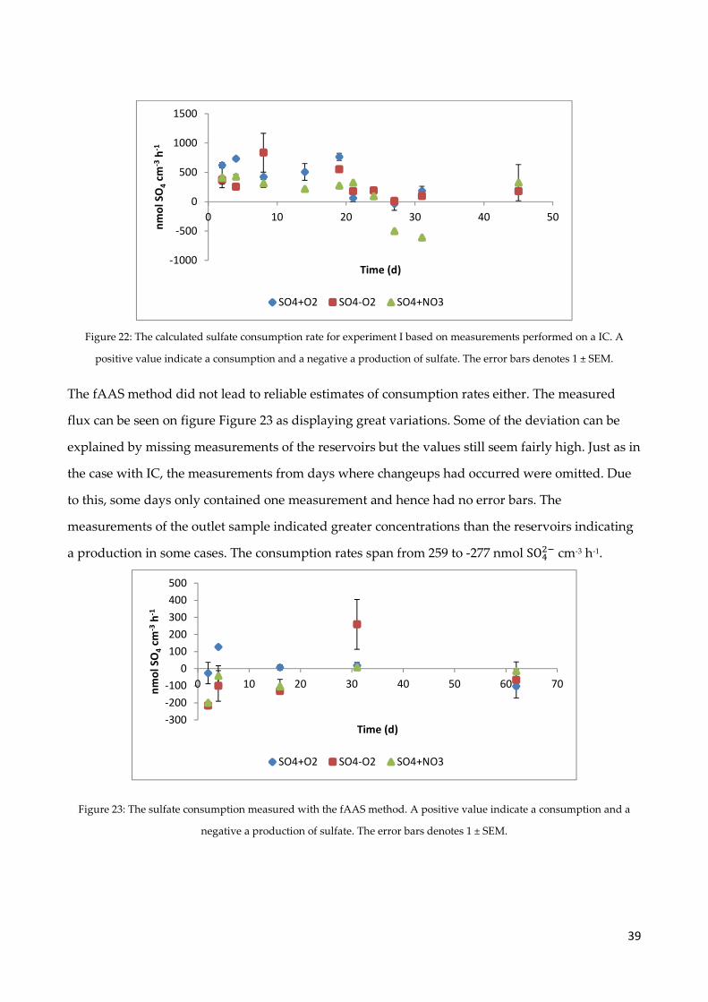
39
Figure 22: The calculated sulfate consumption rate for experiment I based on measurements performed on a IC. A
positive value indicate a consumption and a negative a production of sulfate. The error bars denotes 1 ± SEM.
The fAAS method did not lead to reliable estimates of consumption rates either. The measured
flux can be seen on figure Figure 23 as displaying great variations. Some of the deviation can be
explained by missing measurements of the reservoirs but the values still seem fairly high. Just as in
the case with IC, the measurements from days where changeups had occurred were omitted. Due
to this, some days only contained one measurement and hence had no error bars. The
measurements of the outlet sample indicated greater concentrations than the reservoirs indicating
a production in some cases. The consumption rates span from 259 to -277 nmol SO��� cm-3 h-1.
Figure 23: The sulfate consumption measured with the fAAS method. A positive value indicate a consumption and a
negative a production of sulfate. The error bars denotes 1 ± SEM.
-1000
-500
0
500
1000
1500
0 10 20 30 40 50
nm
ol
SO
4cm
-3h
-1
Time (d)
SO4+O2 SO4-O2 SO4+NO3
-300
-200
-100
0
100
200
300
400
500
0 10 20 30 40 50 60 70
nm
ol
SO
4cm
-3h
-1
Time (d)
SO4+O2 SO4-O2 SO4+NO3

40
Some of the difficulties experienced in experiment I in obtaining reliable consumption rates for
sulfate were improved in experiment II. No changeups in the tubing occurred and the reservoirs
were always measured instead of using an average. Data from the initial phase of the experiment
was more frequently measured compared to later in the experiment. Furthermore, the data was
corrected for dilution or evaporation error with bromide. The concentration of bromide was 10
mM, which had been measured during the bromide break through experiment. The measured net
sulfate consumption and production values from the ion chromatography for experiment II span
from 421 to -1161 nmol SO���cm-3 h-1 (Figure 24). The overall tendency, as was the case with
experiment I, was the data being inconsistent and displaying great variation. The data seem
limited to usefully detect if sulfate had been present in the proper reservoirs and reactors in
sufficient concentrations, but not to reliably estimate rates of consumption or production of sulfate.
Figure 24: The consumption of sulfate for experiment II measured using an ion chromatograph. A positive value indicate
a consumption and a negative a production of sulfate. The line indicates where the flow rate was changed. The error bars
denote 1 ± SEM.
4.8 Carbon dioxide production
The daily carbon dioxide production was measured numerous times for each reactor during both
experiments by the GSIRe method explained and described in section 2.2 and 4.2. The daily
production of carbon dioxide for each treatment for experiment I can be found in Figure 25. To
ensure a clear view of a potential decrease in rates, samples were more frequently analyzed during
the first ten days of the experiment. After this period, the data started to stabilize but still exhibited
some variation. All treatments display an exponential relationship in the investigated timeframe.
-1500
-1000
-500
0
500
1000
0 5 10 15 20 25 30 35 40
nm
ol
SO
4cm
-3h
-1
Time (d)
SO4+O2 SO4-O2 SO4+NO3
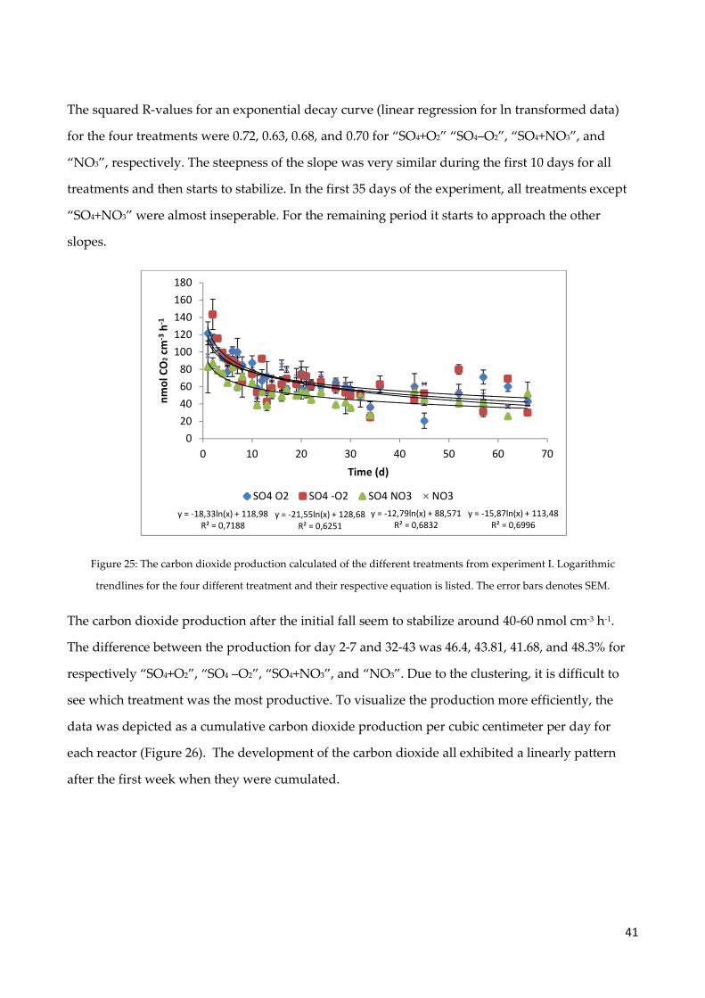
41
The squared R-values for an exponential decay curve (linear regression for ln transformed data)
for the four treatments were 0.72, 0.63, 0.68, and 0.70 for “SO4+O2” “SO4–O2”, “SO4+NO3”, and
“NO3”, respectively. The steepness of the slope was very similar during the first 10 days for all
treatments and then starts to stabilize. In the first 35 days of the experiment, all treatments except
“SO4+NO3” were almost inseperable. For the remaining period it starts to approach the other
slopes.
Figure 25: The carbon dioxide production calculated of the different treatments from experiment I. Logarithmic
trendlines for the four different treatment and their respective equation is listed. The error bars denotes SEM.
The carbon dioxide production after the initial fall seem to stabilize around 40-60 nmol cm-3 h-1.
The difference between the production for day 2-7 and 32-43 was 46.4, 43.81, 41.68, and 48.3% for
respectively “SO4+O2”, “SO4 –O2”, “SO4+NO3”, and “NO3”. Due to the clustering, it is difficult to
see which treatment was the most productive. To visualize the production more efficiently, the
data was depicted as a cumulative carbon dioxide production per cubic centimeter per day for
each reactor (Figure 26). The development of the carbon dioxide all exhibited a linearly pattern
after the first week when they were cumulated.
y = -18,33ln(x) + 118,98
R² = 0,7188
y = -21,55ln(x) + 128,68
R² = 0,6251
y = -12,79ln(x) + 88,571
R² = 0,6832
y = -15,87ln(x) + 113,48
R² = 0,6996
0
20
40
60
80
100
120
140
160
180
0 10 20 30 40 50 60 70
nm
ol
CO
2cm
-3h
-1
Time (d)
SO4 O2 SO4 -O2 SO4 NO3 NO3

42
Figure 26: Cumulative carbon dioxide production of the various treatments for experiment I. Note, the unit of the y-axis
is in µmol cm-3 d-1. The error bars are SEM.
The four treatments display a similar pattern as in Figure 25 for especially the first 20 day where
they seem inseperable. It seems as if “SO4+NO3” produced less carbon dioxide compared to the
other treatments, which even at the end of the experiment followed each other closely. To inspect if
the daily production and the cumulated production of carbon dioxide deviated between
treatments in the experiment, three dates were statistically analyzed.
Figure 27: Panel A: The daily carbon dioxide production at three selected days for all treatments in experiment I. Panel B:
The cumulated production of carbon dioxide at three selected days for all treatments in experiment I. For both panel A
and B the error bars are 1 ± SEM.
0,0
20,0
40,0
60,0
80,0
100,0
120,0
0 10 20 30 40 50 60 70
µm
ol
CO
2cm
-3
Time (d)
SO4+O2 SO4-O2 SO4+NO3 NO3
0
20
40
60
80
100
120
5 34 66
nm
ol C
O2
cm-3
h-1
Time (d)
SO4+O2 SO4-O2 SO4+NO3 NO3
0,0
20,0
40,0
60,0
80,0
100,0
120,0
5 34 66
µm
ol C
O2
cm-3
Time (d)
SO4+O2 SO4-O2 SO4+NO3 NO3
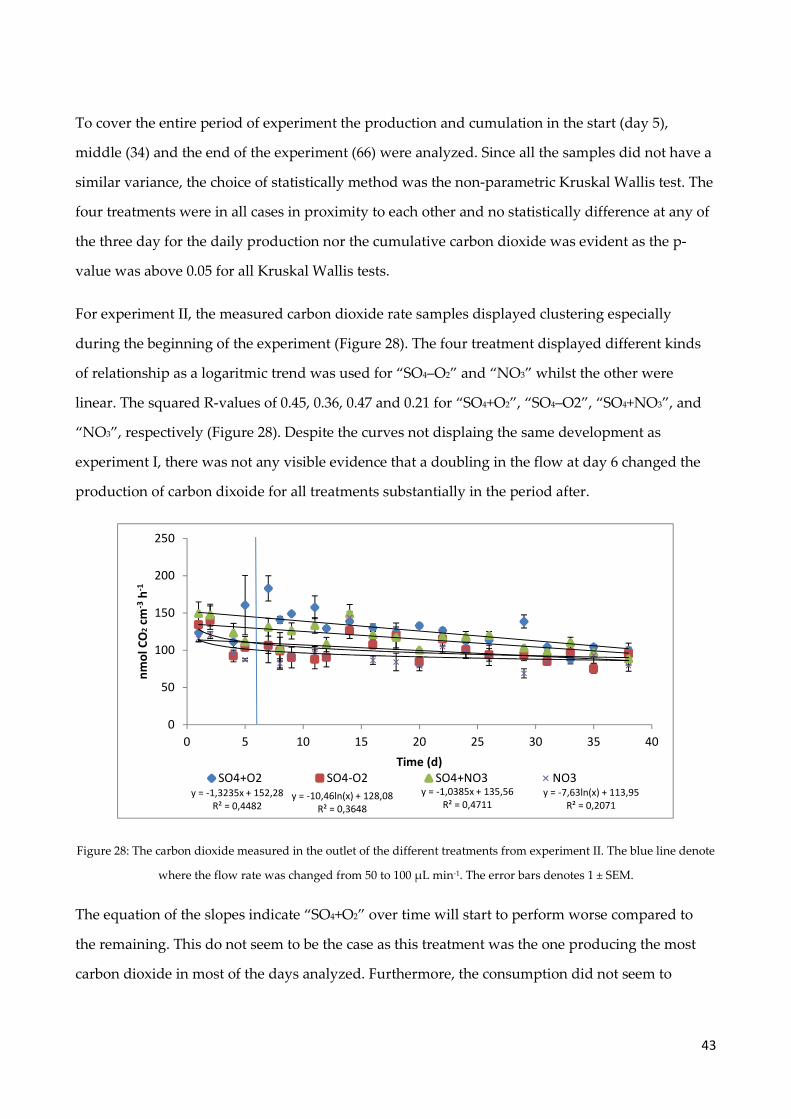
43
To cover the entire period of experiment the production and cumulation in the start (day 5),
middle (34) and the end of the experiment (66) were analyzed. Since all the samples did not have a
similar variance, the choice of statistically method was the non-parametric Kruskal Wallis test. The
four treatments were in all cases in proximity to each other and no statistically difference at any of
the three day for the daily production nor the cumulative carbon dioxide was evident as the p-
value was above 0.05 for all Kruskal Wallis tests.
For experiment II, the measured carbon dioxide rate samples displayed clustering especially
during the beginning of the experiment (Figure 28). The four treatment displayed different kinds
of relationship as a logaritmic trend was used for “SO4–O2” and “NO3” whilst the other were
linear. The squared R-values of 0.45, 0.36, 0.47 and 0.21 for “SO4+O2”, “SO4–O2”, “SO4+NO3”, and
“NO3”, respectively (Figure 28). Despite the curves not displaing the same development as
experiment I, there was not any visible evidence that a doubling in the flow at day 6 changed the
production of carbon dixoide for all treatments substantially in the period after.
Figure 28: The carbon dioxide measured in the outlet of the different treatments from experiment II. The blue line denote
where the flow rate was changed from 50 to 100 µL min-1. The error bars denotes 1 ± SEM.
The equation of the slopes indicate “SO4+O2” over time will start to perform worse compared to
the remaining. This do not seem to be the case as this treatment was the one producing the most
carbon dioxide in most of the days analyzed. Furthermore, the consumption did not seem to
y = -1,3235x + 152,28
R² = 0,4482y = -10,46ln(x) + 128,08
R² = 0,3648
y = -1,0385x + 135,56
R² = 0,4711
y = -7,63ln(x) + 113,95
R² = 0,2071
0
50
100
150
200
250
0 5 10 15 20 25 30 35 40
nm
ol
CO
2cm
-3h
-1
Time (d)
SO4+O2 SO4-O2 SO4+NO3 NO3

44
decrease as it did with nitrate (see Figure 20). The reason for the steeper slope was due to it
performing exceptionally better in the beginning and then start to decrease rather suddenly. For
the latter part of the experiment, there was a steady decrease in productivity. It was therefore
likely a poor fitting of the curve due to high measurements of the initial days that caused this. For
all treatments, a loss in productivity was observeable. The difference in the rate of the four
treatments for the first four days and the last 3 days result in a loss of productivity of 22.71, 25.61,
29.59, and 20.62% for respectively “SO4+O2”, “SO4-O2”, “SO4+NO3”, and “NO3”. This decrease from
start to end was not as steep as experiment I, but still evident. To visualize the productivity over
the course of the experiment a cumulative carbon dioxide graph was made (Figure 29).
The cumulative carbon dioxide production during the entire period displayed a linear relationship
for all treatments. The development was strikingly similar for the first 6 days where all treatments
seem inseperable. Around day 18 the lines begin to separate themselves in an sequence in which
did not change throughout the experiment. The ranking of the most productive from the top was
“SO4+O2”, “SO4+NO3”, “SO4 –O2”, and finally “NO3”. From day 28 and onwards the productivity
began to decrease resulting in a bending of the lines. The difference between the treatments only
seem to increase over time.
To inspect if the daily production and the acumulated carbon dioxide production varied for the
different treatments during the experiment three selected days were statistically analyzed. The
three selected days were one from the start (4), middle (20) and end of the experiment (38).
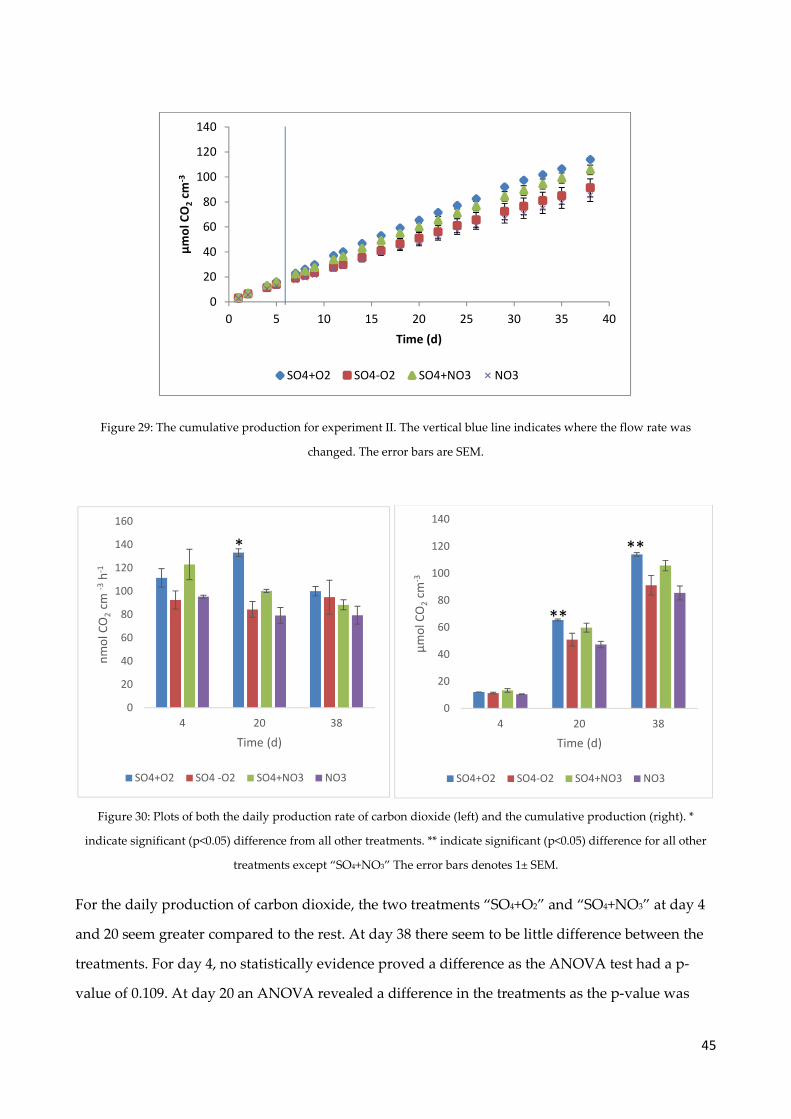
45
Figure 29: The cumulative production for experiment II. The vertical blue line indicates where the flow rate was
changed. The error bars are SEM.
Figure 30: Plots of both the daily production rate of carbon dioxide (left) and the cumulative production (right). *
indicate significant (p<0.05) difference from all other treatments. ** indicate significant (p<0.05) difference for all other
treatments except “SO4+NO3” The error bars denotes 1± SEM.
For the daily production of carbon dioxide, the two treatments “SO4+O2” and “SO4+NO3” at day 4
and 20 seem greater compared to the rest. At day 38 there seem to be little difference between the
treatments. For day 4, no statistically evidence proved a difference as the ANOVA test had a p-
value of 0.109. At day 20 an ANOVA revealed a difference in the treatments as the p-value was
0
20
40
60
80
100
120
140
0 5 10 15 20 25 30 35 40
µm
ol
CO
2cm
-3
Time (d)
SO4+O2 SO4-O2 SO4+NO3 NO3
0
20
40
60
80
100
120
140
160
4 20 38
nm
ol C
O2
cm -3
h-1
Time (d)
SO4+O2 SO4 -O2 SO4+NO3 NO3
*
0
20
40
60
80
100
120
140
4 20 38
µm
ol C
O2
cm-3
Time (d)
SO4+O2 SO4-O2 SO4+NO3 NO3
**
**
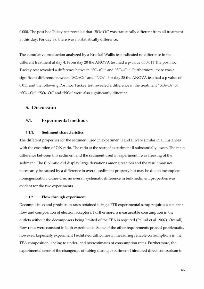
46
0.000. The post hoc Tukey test revealed that “SO4+O2” was statistically different from all treatment
at this day. For day 38, there was no statistically difference.
The cumulative production analyzed by a Kruskal Wallis test indicated no difference in the
different treatment at day 4. From day 20 the ANOVA test had a p-value of 0.011 The post hoc
Tuckey rest revealed a difference between “SO4+O2” and “SO4–O2”. Furthermore, there was a
significant difference between “SO4+O2” and “NO3”. For day 38 the ANOVA test had a p value of
0.011 and the following Post hoc Tuckey test revealed a difference in the treatment “SO4+O2” of
“SO4 –O2”. “SO4+O2” and “NO3” were also significantly different.
5. Discussion
5.1. Experimental methods
5.1.1. Sediment characteristics
The different properties for the sediment used in experiment I and II were similar in all instances
with the exception of C:N ratio. The ratio at the start of experiment II substantially lower. The main
difference between this sediment and the sediment used in experiment I was freezing of the
sediment. The C:N ratio did display large deviations among reactors and the result may not
necessarily be caused by a difference in overall sediment property but may be due to incomplete
homogenization. Otherwise, no overall systematic difference in bulk sediment properties was
evident for the two experiments.
5.1.2. Flow through experiment
Decomposition and production rates obtained using a FTR experimental setup requires a constant
flow and composition of electron acceptors. Furthermore, a measureable consumption in the
outlets without the decomposers being limited of the TEA is required (Pallud et al. 2007). Overall,
flow rates were constant in both experiments. Some of the other requirements proved problematic,
however. Especially experiment I exhibited difficulties in measuring reliable consumptions in the
TEA composition leading to under- and overestimates of consumption rates. Furthermore, the
experimental error of the changeups of tubing during experiment I hindered direct comparison to

47
experiment II of all but one treatment (SO4+O2) and one reactor in the treatment “SO4+NO3”. For
experiment II, these problems were with the exception of sufficiently sulfate measurements solved,
and the focus in this section will thus mainly be on the result from experiment II.
Both experiments exhibited leakage when sediment was inserted in the reactors. The
measurements for the experiments were not started until this leakage was stopped. This took
roughly four days for both experiments causing the experiment to run without collection of
samples in this period. In this phase of experiment II, the water in the outlets displayed a tinge of
yellow. Leaching of organic material was presumably evident in this phase meaning a portion of
the decomposable organic material (e.g., protein, carbohydrates) was probably flushed and
thereby lost in the initial phase of the experiment, possibly before any measurements were made.
This would theoretically decrease the overall decomposition rate, as less labile organic matter
would be available. This possible leaching of a labile fraction was not directly verified, as the water
was not sampled until the leakage was stopped. The reason for this leaching was may have been
due to the freezing of the sediment, which could have caused a release and loss of the labile
fraction of the organic matter, especially at the start of the experiment. Andersen (1996) found that
freezing and subsequently thawing diatoms lead to a loss of 32% of labeled carbon due to
disruption of cell walls. It is noteworthy that the changes in decomposition rates over the course of
the second experiment were much less resulting in more stabilized curves compared to the first
experiment supporting the idea that an initial more labile fraction, with associated rapid
decomposition was indeed missed.
The flow inside the reactors were investigated by a break through experiment where bromide
worked as an inert tracer. For experiment I with a nominal flow of 40 µL m-1 the breakthrough
time was ~23 hours. For experiment II the nominal flow was 100 µL m-1 the breakthrough ~11
hours. The two experiments displayed good agreement between the reactors concerning the
breakthrough time and the values obtained for the longitudinal dispersion coefficient was similar
to the values obtained in (Roychoudhury et al. 1998). The number of times pore volume had to be
flushing through the reactors to change all water (2.97-3.21) and thereby obtain a new steady state
was similar to the numbers found in the study by Pallud et al. (2007). No differences in the water
flow could be detected for all reactors in both experiments.

48
In contrast to other FTR experiments, the sediment used in these experiments was homogenized
by hand before insertion in the reactors (Laverman et al. 2012; Pallud et al. 2007; Pallud & Van
Cappellen 2006). The sediment used was therefore more disturbed in comparison to these
experiments and this may alter e.g. reaction kinetics. The measured values obtained in this study
do therefore not necessarily reflect in situ rates to same degree in these other FTR experiments
(Pallud et al. 2007; Pallud & Van Cappellen 2006).
5.1.3. Measurements of nitrate
A Lachat flow injection analyser was used for measurements of nitrate samples for both
experiment and these were by far the most reliable measurement of TEA used in these
experiments. The results proved to be accurate and precise and the method was therefore
considered sufficient to determining nitrate consumption rates for both experiment as illustrated
in Figure 19 and Figure 20. For future experiments, this method for measuring nitrate consumption
is therefore strongly recommended.
5.1.4. Measurement of oxygen
Obtaining reliable measurements of oxygen for the anaerobic treatments proved challenging and
was first satisfied when a glove bag was continuously supplied with nitrogen gas. Until this step
was implemented at day 21, the outlets for the anaerobic treatments were to various degrees
oxygenated. For experiment I, where the bag was inflated in the evening only, the oxygen content
in the outlets for the anaerobic part averaged using all available days was 12.3% ± 0.96%. In
experiment II, where nitrogen gas was supplied continuously, levels were 2.1% ± 1.09%, and
include two days the bag was not inflated properly and oxygen had diffused into the collectors.
Continuously supplying the glove bag with nitrogen gas enabled low oxygen content in the glove
bag and is highly recommended for future experiments.
One of the factors identified in the methodical handling of the oxygen to influence the
measurement of oxygen, was the absence or presence of an overflow in the collectors. The
importance of overflow in the collectors was rendered visible by analysis of the initial samples of
experiment II (Figure 21). Before the flow rate was increased in experiment II, the collectors did not
at all times display an overflow of water. After the flow rate was increased, the overflow was with
a few exceptions at all times present in all treatments. When comparing the oxygen consumption
49
rate for “SO4+O2” before and after the flow rate was changed, the consumption rate seemed to
drastically increase. This change was not caused by the change in flow rate, as the consumption
rate measured on the sixth day was similar to the later days. On this day, all outlets in the
treatment “SO4+O2” contained an overflow. On the fifth day of the experiment, none of the outlets
contained any overflow, and the consumption of oxygen approached values of 0 nmol cm-3 h-1.
This proved generating an overflow was of vital importance, if a precise evaluation of the oxygen
consumption was needed, presumably because the water sampled for oxygen determination was
better protected from contamination via this overflow.
Not all the low consumption rates of oxygen observed from experiment I could be accredited to a
lack of overflow in the outlets, however. An overflow was consistently generated during
experiment I but the outlets proved little or none consumption of oxygen during the entire period
(see Figure 21). The reason for the lack of oxygen consumption was identified as the choice of
tubing. For the entire experiment I, silicone tubes were used for all tubing. Silicone tubes are
permeable and the potential diffusion of oxygen across the tube lead to an underestimate in the
consumption rate, despite the relatively short (~1 h) in the tubes from the reactors to the collectors.
For experiment II, less permeable Viton tubes were utilized resulting in measureable consumption
rates. To obtain accurate and reliable oxygen measurements, both creating an overflow and the use
of gas impermeable tubes were crucial improvements making the results from experiment II
reliable and are highly recommended for future experiments.
5.1.5. Measurement of sulfate
An alternative method for measuring sulfate in aqueous solutions using fAAS was presented in
this study. Preparation of the samples was found to be most precise after cooling of the samples
(Figure 8). Centrifuging the samples was visually observed to enhance the precipitation and the
combination of cooling and freezing is suggested for future experiments. The fAAS method
contain three major advantages. First, water samples taken in the field can be prepared for analysis
directly, transported to a refrigerator, and stored for a day before measurements. Second, the
samples are rapidly analyzed. This means that up to three digits of samples per day could easily be
prepared. Third, reagents other than diluted hydrogen chloride (0.005 M), deionized water, and a
stock solution of barium chloride are not needed, causing the method to be relatively safe and

50
economical. The reagents do not require handling beforehand, which make it even easier bringing
into the field. The method was tested using various concentration of sulfate and was in one
experiment found to underestimate the sulfate concentration and another to overestimate the
sulfate concentration by approximately 10% (see Figure 7 and Figure 8). The reason for the
changing deviation in the measurements requires further study if the method is to be
implemented.
The fAAS barium sulfate method and IC were used for analysis of sulfate in the samples. Both
methods were limited in performing accurate and precise enough measurement for determination
of the sulfate consumption rates, as the deviation in the measured samples was too great compared
to the expected change in sulfate concentration(see Figure 22, Figure 23 and Figure 24). Both
negative and positive consumptions rates of sulfate were measured. While a production of sulfate
could occur through oxidation of hydrogen sulfide by oxygen or nitrate (Laverman et al. 2012);
Canfield et al. 2005) this would not be expected in the “SO4-O2” treatment, for example.
Furthermore, the measured sulfate production was several times greater than the supplied amount
of nitrate and oxygen and an oxidation of that level is impossible. Expected maximum sulfate
reduction rates for saltmarsh sediment, based on earlier studies performed by (Pallud et al. 2007;
Pallud & Van Cappellen 2006; Laverman et al. 2012) is around 10-49 nmol cm-3 h-1 and such rates
would translate to sulfate consumptions of 65.6 µM to 330 µM at this flow setup. Reliably
measurement of such small changes was beyond the capabilities of either of the techniques used
here.
The sulfate data from both experiments did, however indicate if sulfate had been present in the
right reactors and in the proper concentration throughout the experiment. Furthermore, based on
these sulfate measurements it was obvious several tubes experienced changeups during
experiment I (confer 4.5), while this did not occur for experiment II. The large deviation in the
measurements unfortunately hindered a realistic stoichiometric comparison between the
production of carbon dioxide and the consumption of sulfate concentration for both experiments,
however. But the decomposition estimated from carbon dioxide production in these treatments
should reflect that occurring with sulfate available.

51
5.1.6. Measurement of carbon dioxide
An alternative method to the tedious Gran titration for measuring aqueous carbon dioxide was
desirable for this experiment as hundreds of carbon dioxide samples were to be analyzed. This
resulted in a new method of measuring carbon dioxide using a gas sensor operating with an IR-
electrode. The GSIRe was investigated and optimized in several aspects through numerous
experiments (confer section 4.2). The method prove capable of producing results concordant with
the Gran titration for concentrations in the range of 0 to 5 mM sodium carbonate (Figure 16). Based
on the slope of the regression lines from data from the two methods it seems plausible the results
at higher than 5 mM would agree similarly. The advantages of this method is that it is less effort
demanding, easy operational, and capable of measuring carbon dioxide for a wide range (0-20
mM). The method was similar to Gran titration in the time required per sample. Due to the
calibration of the electrode, the number of samples measured per day was less than what could be
done by Gran titration. The GSIRe method provided precise and accurate measurement of carbon
dioxide from an aqueous sample and can easily be utilized for future experiments.
5.2. Consumption rates of various TEA
5.2.1. Nitrate consumption rate
For experiment I, the daily nitrate consumption for the entire experimental period was stable. The
mean of the “SO4+NO3” and “NO3” was 9.75 ± 0.51 and 10.73 ± 0.61 nmol cm-3 h-1. The low
availability of nitrate in experiment I caused exhaustion of nitrate, thereby limiting measurement
of the consumption rate, which was underestimated in the start of the experiment. Changeups at
different times in the experiment probably had an additional effect on the measured rate, but this
effect is difficult to quantify.
In the initial phase of experiment II before the flow rate was changed, the decomposers may have
experienced low availability of nitrate as the mean consumption for the treatments “SO4+NO3” and
“NO3” were 421 ± 10.0 µM and 441.5 ± 13.8 µM out of the 500 µM reservoir. The only difference at
this point between the setup of experiment I and experiment II was a small increase in the flow
rate and an increase in the reservoir nitrate concentration. The measurements of the initial days
confirmed the suspicion that the decomposers had been influenced by low availability of nitrate.
52
This occurred at least in the initial phase of experiment I as the consumption in the experiment II
during the initial days exceeded the reservoirs concentration in experiment I. Even with twice the
nitrate concentration, the consumption rates were so great and the availability in the outlet so low
it seems plausible the consumption rate could have been substantially higher in the initial days of
experiment II if more nitrate was available.
After the initial phase of experiment II, the consumption rate of nitrate displayed a steep decrease
in the middle of the experiment. For the first fourteen days of the experiment, the mean
consumption of “SO4+NO3” and “NO3” was 33.9 ± 1.31 and 29.8 ± 1.64 nmol NO�� cm-3 h-1. For the
remaining of experiment II, the two treatments had much lower consumption rates with means of
6.9 ± 0.40 and 7.6 ± 1.48 nmol NO�� cm-3 h-1. The drop in consumption rate could be caused by the
labile fraction being exhausted. The daily carbon dioxide production did not, however, reflect this
change as those rates remained more or less unchanged (see 5.3.1). If nitrate was consumed but not
used for nitrate reduction, another explanation for the sudden decrease could be a net
immobilization of nitrogen by the decomposers (Canfield et al. 2005). Both explanations seem
plausible and can not be excluded based on the data from this study.
Assuming that the nitrate reduction is limited to the upper 10 cm in the sediment column, the
mean volumetric rates of nitrate consumption corresponds to depth-integrated areal rates of 57.12
and 51.5 for“SO4+NO3” and “NO3” in experiment II. An example of this calculation can be found in
the appendix. Jørgensen & Sørensen (1985) measured nitrate reduction rates ranging from around
2 to 50 mmol m-2 d-1 and thus the estimated rates in experiment II are quite high. If, however, the
active nitrate reduction zone is less than 10 cm deep, the integrated areal rates would also be
proportionally lower.
The mean consumption rate for the entire experiment II for “SO4+NO3” and “NO3” were 23.8 ± 3.48
and 21.5 ± 3.00 nmol NO�� cm-3 h-1, respectively. Laverman et al. (2006) measured maximum rate of
nitrate reduction ranged from 100 to 325 nmol cm-3 h-1 using sediment from the first centimeter of a
lower estuary sediment. Pallud & Van Cappellen (2006) found values of 300-600 nmol cm-3 h-1 in
freshwater estuary sediment. As their consumption rates were far greater than the values obtained
in this study, it seem plausible the Km constants in the experiments presented here were
substantially lower. The similar consumption rates for experiment I and II in the end of the

53
experiment where neither seem nitrate limited support this hypothesis. This was somewhat
unexpected as experiment II received twice the concentration as experiment I and ran at a higher
flow rate. If a surplus of decomposable organic material was at disposal, a greater consumption
rate was expected if the TEA had been limited in experiment I unless the decomposers were
operating under a situation where they were in fact not nitrate limited. As the consumption rate
was actually slightly lower for experiment II compared to the first, indications are that the limiting
factor concerning the decomposition of the organic matter through various nitrogen pathways is
the initial hydrolysis of organic matter. The finding was in accordance with Kristensen & Holmer
(2001) who found that the limiting step for aerobic and anaerobic decomposition (including nitrate
reduction) to be the initial hydrolytic attack on the complex particulate remains of the organic
matter. The data obtained in this study does not allow for determination of whether this is the
mechanism here. It does, however, seem that nitrate reduction rates were not influenced by the
nitrate availability in most of the time, especially for experiment II, and thus must be limited by the
availability of degradable organic substrate.
5.2.2. Oxygen consumption rate
The measured oxygen consumption rate of experiment I falsely indicated virtually no
consumption throughout the experiment (see Figure 21). The reactor did probably exhaust all
oxygen, causing anoxic conditions. The colour of the sediment after completion of the experiment
supports this hypothesis as the reactor contained a great portion of black areas both inside and
outside the reactors indicating anoxic conditions. The reason why the measurements did not
indicate this was due to diffusion of oxygen into the silicone tubing thereby re-oxygenating the
water (see 5.1.4). Black areas were evident in the reactor for experiment II but to a less degree,
indicating improved oxygenation of the sediment.
The mean consumption rate of oxygen from the treatment “SO4+O2” of experiment II from day 7 to
38 were 15.79 ± 0.80 nmol cm-3 h-1. Day 1 to 6 were not included due to a general lack of overflow in
the outlets causing a gross underestimation of the oxygen consumption. The consumption
throughout the experiment was stable and did not decrease in a similar fashion as the nitrate
consumption, although oxygen consumption rates were somewhat lower on average. Comparing
to the other TEA consumption rates, it is likely that oxygen consumption rates were still
54
underestimated in experiment II. It is expected that aerobic decomposition should be the same or
faster than anaerobic decomposition, but not markedly slower. The reason for this deviation could
be linked to low availability of oxygen. Oxygen limitations in natural microbial communities occur
in the few micromolar range. If that holds true, the decomposers were probably not limited by
oxygen throughout experiment II (Canfield et al. 2005). A complete exhaustion of the oxygen did
not occur and the decomposers are thought to be supplied with sufficient oxygen to uphold high
rates. Hansen & Blackburn (1991) found using a different flow system an initial oxygen
consumption of 63 mmol m-2 d-1. The data in this study had an estimated consumption rate of 7.57
mmol m-2 d-1, which is much lower than the previously mentioned nitrate. This was under the
assumption that the oxic respiration only occurred in the first 2 cm. The reason for the deviation
between this study and Hansen & Blackburn (1991) could be caused by different history of the
sediment amongst others but is most likely due to the issues with measuring accurate rates of
oxygen consumption in this flow-through system.
5.2.3. Sulfate consumption rate
The sulfate concentration in the outlets was measureable using both the fAAS method and the IC.
The consumption rate proved unreliable as the measurements contained great deviations in the
rate calculated as seen on Figure 22, Figure 23, and Figure 24. Sulfate consumption rate has been
measured successfully in FTR experiments by others. Pallud & Van Cappellen (2006) measured
maximum sulfate reduction rates of 27.7 nmol SO��� cm-3 h.1 and a Km of 0.1 mM from sediment
from a salt marsh from depths of 2-4 centimeter. No large difference in the rate was found between
0-6 cm. Pallud et al. (2007) found maximum sulfate reduction rate of 33.10 nmol SO��� cm-3 h-1 and
Km of 0.25 mM in the same salt marsh but at a depth of 0 to 2 cm. Both were incubated at 21˚C,
which was very close to the temperature used in this study. As the concentration of sulfate in this
study was far above the listed Km value, the reactors should have received sufficient amounts of
sulfate to sustain a maximum sulfate reduction rate. In comparison the nitrate consumption rate
obtained in this study did also differ from their nitrate reduction rate. The development of “SO4-
O2”, however, was similar to the other treatments for both experiments indicating a similar
consumption rate as to the ones found in the nitrate treatments. The reason why other researches
were capable of measuring sulfate was probably that the groups used lower concentrations of
sulfate so the relative change in sulfate was much larger than what was measured in this study. As
55
mentioned earlier, the theoretical sulfate consumption constituted less than 2 % of the total sulfate
concentration in the reservoirs. Pallud et al. (2007) and Roychoudhury et al. (1998) suggest in their
studies to use concentration ranges where the difference in concentration between the reservoir
and the outlet can be detected. Either decreasing the sulfate concentration or prolonging the
residence time would most likely improve the sulfate measurements but further investigation is
nequired to clarify this.
5.3. Daily carbon dioxide production rate
5.3.1. Carbon dioxide production from nitrate consumption
Comparison of results found in this study to result from other studies is challenging as the TEA
supplied, history and quality of the sediment differed between the different studies. As mentioned
earlier, only one reactor outside the aerobic part of the experiment did not experience any change
up in experiment I (SO4+NO3 2). The productivity of carbon dioxide for this treatment at day 30-34
was 36.18 ± 6.06 nmol cm-3 h-1. The development of the two treatments containing nitrate was very
similar for experiment II. The development was stable and did not decrease throughout the
experiment. The decrease in nitrate consumption during experiment II was not reflected in the
carbon dioxide production, which for “SO4+NO3” and “NO3” the first 14 days were 129.7 ± 5.47
and 102.4 ± 5.96 nmol cm-3 h-1. The remaining part of the experiment it was 108.1 ± 3.42 and 87.6 ±
3.02 nmol cm-3 h-1.
Other researchers have investigated nitrate pathways using a FTR experimental setup (Laverman
et al. 2006; Pallud et al. 2007). Pallud et al. (2007) found that the nitrate reduction rates was
approximately 180 nmol cm-3 h-1 at steady state using sediment taken from a freshwater area at
depths of 0-1 cm and run at 6 mL h-1 and supplied with 2.5 mM. The corresponding carbon dioxide
production was estimated to 93-265 nmol cm-3 h-1. As mentioned earlier in the discussion, it is
believed nitrate at least in the end of experiment I and II was present in such concentrations that it
was not limiting. As nitrate was not completely exhausted in the initial 14 days where the
consumption rate was at its highest, it seems unlikely the difference between this study and Pallud
et al. (2007) was due to the supply of nitrate. Instead, differences in the rates between these
experiments and others were correlated to the sediment. The previous mentioned studies utilized
56
sediment from less deep layers than the ones used here and a larger portion of the labile fraction
might therefore be available. Furthermore, the sediment used in this study was stored in the
climate room for weeks before usage and this could affect the quantity of the labile pool, which in
turn would likely decrease the rate of decomposition labile portion.
5.3.2. Carbon dioxide production from oxygen consumption
The “SO4+O2” treatment in experiment I measured virtually no oxygen consumption but was still
considered to have anoxic conditions in the reactors. This has influenced the carbon dioxide
production as not all of it was produced through oxic respiration. Sulfate reduction probably
occurred when oxygen, due to the oxic respiration or oxidation of other TEAs, was exhausted
(Canfield et al. 2005). The daily production rate of carbon dioxide was for the first four days
initially 109.4 ± 5.92 nmol cm-3 h-1 for experiment I and 126.21 ± 7.74 nmol cm-3 h-1 for the second
(see Figure 25 and Figure 28). During the initial days, the only difference between the two
experiment, other than the freezing and thawing of the sediment was a small increase in the flow
rate. The average production rate of carbon dioxide of day 34-36 of experiment I was 48.17 ± 6.58
nmol cm-3 h-1 and averaged over day 33-38 the rate for experiment II was 97.55 ± 10.21 nmol cm-3 h-
1.
5.3.3. Carbon dioxide production from sulfate consumption
One reactor in “SO4-O2” was the only TEA treatment that was tested without issues in both
experiments. Thus, these results are the best way to compare overall differences between the two
experiments. The mean carbon dioxide production rate for this reactor from day 2 to day 6 was
104.2 ± 7.46 nmol cm-3 h-1 and for day 32-36 it was 43.2 ± 8.4 nmol cm-3 h-1 in experiment I. The three
reactors of the “SO4–O2” treatment from experiment II had a mean production of carbon dioxide of
115.49 ± 5.4 nmol cm-3 h-1 from day 1 to 5 and 85.44 ± 3.77 nmol cm-3 h-1 from day 31-35 (see Figure
28). There was no difference during the initial days but over time, the productivity decreased
strongly for the reactor in experiment I whilst the other reactors had a far smaller decline.
5.3.4. Stoichiometry
The consumption of the various TEAs and the production of carbon dioxide displayed a noteable
incongruence as the production of carbon dioxide in the end of the experiment well exceeded the
consumption of the TEAs. To evaluate the stoichiometric in the experiments, the respiratory

57
quotient (RQ) for the different treatments was calculated by dividing the overall mean production
rate from each carbon dioxide production by the respective mean consumption rate taken over all
days (Table 4) (Hansen & Blackburn 1991). Ideally, the RQ ratio for the different treatment is
located around a value of 1-2 dependent of the terminal electron acceptor.
Table 4: The respiratory quotient (RQ) for the different treatments. The treatments that experienced a changeup during
experiment I were discarded and the remaining one were used. “SO4 –O2” could not be calculated as the consumption
rate for sulfate was immeasurable.
Treatment Theoretical RQ experiment I RQ experiment II
SO4+O2 1 127.0 9.6
SO4 -O2 2 N/A N/A
SO4+NO3 1.25-2 5.88 4.94
NO3 1.25 6.49 4.40
For all treatments for both experiments, the RQ ratio deviated substantially from the ideal values.
The RQ value for the treatment “SO4+O2” for experiment I exhibited a staggering value of 127 but
was falsely contributed due to virtually no consumption of oxygen (see Figure 21). The RQ values
from the table indicate a sulfate reduction in the treatment “SO4+NO3” for experiment II as there
was a lower RQ ratio for the “SO4+NO3” compared to the “NO3” treatments. The “SO4+NO3” and
“NO3” treatments might have had insufficient levels of nitrate to exclude other decomposers at
times in experiment II. The production of carbon dioxide may have occurred through other
electron acceptors (e.g. sulfate and methanogenesis) thereby decreasing the RQ ratio. Methanogens
gets favorable conditions when all other TEA are exhausted (Canfield et al. 2005), and was clearly
not the case in “SO4+NO3” but could potentially have occurred in “NO3” during experiment I. In
most cases, however neither sulfate reduction nor the methanogenesis were thought to account for
the remaining excess of carbon dioxide production and another source of carbon that had not been
accounted for was sought.
5.3.5. Dissolution of CaCO3
A source of carbon, which until this point had not been given any attention so far was the potential
dissolution of calcium carbonate (CaCO3). Other experiments have found it to be contributing to

58
various degree in the total carbon dioxide production (Pallud et al. 2007; Hulthe et al. 1998; Green
& Aller 1998). To verify if calcium carbonate could potential be causing the excessive production of
carbon dioxide, spot checks of calcium concentration in samples from the outlet and the reservoir
was measured on the IC. The measurements indicated calcium to be present in concentrations
(±Sd) of 0.97 ± 0.28 mM for experiment II at day 2 to 4, and 0.52 ± 0.14 at day 9. As no calcium was
added to the reservoirs water, the dissolution of the calcium carbonate in the sediment must be the
source of the calcium. The mean concentration change of carbon dioxide for all treatments in
experiment II was 0.88 ± 0.024 mM and the production of carbonate from the dissolution of CaCO3
could explain 59-108% of the carbon dioxide production. A production of 100 % was, however
rather unlikely as a measurable consumption of nitrate and oxygen had been measured. Using the
data from the IC, the contribution of the calcium on a daily basis was for day 2-4 corresponding to
62% whilst it for day 9 was 68 %. Whatever the value, it is clear that CaCO3 dissolution played a
large role in the carbon dioxide production rates.
The sulfate data on the IC had earlier varied considerably and may not be very precise, thus
adding some doubt to the precision of the calcium determinations on the same apparatus.
Furthermore, it was decided to calculate the solubility of calcium from pH measurements of the
outlets for two specific days as an alternative way of estimating the dissolution of CaCO3. The
calculation for this is found in the appendix. The solubility of calcium, relative to CaCO3, is
indirectly dependent on the pH of the solution as the concentration of carbonate changes as a
function of pH (Figure 31). There was a lower pH in the “SO4+O2” treatment compared to the other
treatments, but the average pH of all the values from a specific sample day was selected for the
calculations. The difference in pH for the “SO4+O2” was probably due to the protons generated in
the oxic respiration, causing the pH to decrease and more CaCO3 to dissolve.
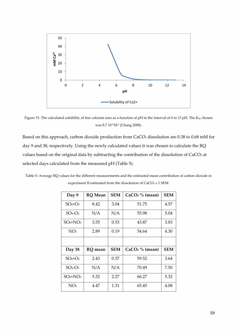
59
Figure 31: The calculated solubility of free calcium ions as a function of pH in the interval of 6 to 13 pH. The Ksp chosen
was 8.7 10-9 M-2 (Chang 2008).
Based on this approach, carbon dioxide production from CaCO3 dissolution are 0.38 to 0.68 mM for
day 9 and 38, respectively. Using the newly calculated values it was chosen to calculate the RQ
values based on the original data by subtracting the contribution of the dissolution of CaCO3 at
selected days calculated from the measured pH (Table 5).
Table 5: Average RQ values for the different measurements and the estimated mean contribution of carbon dioxide in
experiment II estimated from the dissolution of CaCO3 ± 1 SEM.
Day 9 RQ Mean SEM CaCO3 % (mean) SEM
SO4+O2 8.42 3.04 51.75 4.57
SO4-O2 N/A N/A 55.98 5.04
SO4+NO3 3.55 0.53 43.87 3.83
NO3 2.89 0.19 54.64 4.30
Day 38 RQ mean SEM CaCO3 % (mean) SEM
SO4+O2 2.43 0.37 59.52 3.64
SO4-O2 N/A N/A 70.49 7.50
SO4+NO3 5.32 2.27 66.27 5.32
NO3 4.47 1.31 65.45 4.08
0
10
20
30
40
50
0 2 4 6 8 10 12 14
mM
Ca
2+
pH
Solubility of Ca2+

60
The RQ ratios calculated using the estimated contribution of CaCO3 for experiment II generated
lower RQ values (see Table 5). The reason for the large increase in RQ values for the nitrate
containing treatment between the two days was caused by a high consumption rate in the initial
days compared to those at the end of the experiment. As the corrected RQ values were incapable of
reflecting this and the estimated values still deviated considerable it seems likely that even though
the CaCO3 was estimated to contribute 58.5 ± 3.09 % this was an underestimate. Other studies have
encountered the problematics of CaCO3. Pallud et al. (2007) found that dissolution of calcium
carbonate accounted for 39 ± 10% of the export of total dissolved inorganic carbon. Hulthe et al.
(1998) found it to have a maximum production of 7% of the carbon dioxide production. Green &
Aller (1998) found undersaturation of calcium carbonate during winter causing a dissolution that
could account from 20 to 50% of the carbon dioxide production. It needs to be stated that the
assumptions behind the estimations based on the pH calculations (identical pH, specific Ksp and no
interaction of different ions on the solubility) of the production of carbon dioxide from the CaCO3
caused some uncertainties as only a limited amount of the regulating factors were measured in this
study. Due to the possible underestimation of the carbon dioxide production from the CaCO3, the
discussion regarding the carbon dioxide production will be focused on the data found in section
4.8. The absolute numbers in the cumulative production were limited in their usage as the
contribution of carbon dioxide from the dissolution of CaCO3 was impossible to calculate
satisfactorily. The development of the cumulative carbon dioxide for the different treatments
concerning their relative difference still provide an insight in the pattern between the four
treatments, especially given CaCO3 dissolution was likely similar in all treatments. The two
experiments revealed different patterns for the daily production rates of carbon dioxide of the
various treatments.
5.3.6. Kinetics of CaCO3
The four treatments in experiment I displayed a negative exponentially pattern to the carbon
dioxide production rates throughout the experiment. The average decrease in daily carbon dioxide
production rate from the start (day 2-7) to the middle (day 32-43) was 48.15 % ± 3.01 % The
steepest decline occurred within the first 10 days of the experiment, and ensuing the rate steadily
decreased after this point. The drop in productivity in experiment I bear resemblance of a
decomposition of a labile fraction (G1). In the initial phase of the experiment, the decomposers

61
should have a preference of the labile fraction (Canfield et al. 2005). This portion was probably still
remaining causing the decomposers to utilize this first. This could cause an acidification of the
water due to the production of carbonic acid causing the pH to decrease resulting in a larger
dissolution of CaCO3 After approximately 10 days, the labile fraction seemed to be exhausted as
the rate decreased and the production stabilized.
Experiment II displayed a decrease in the daily carbon dioxide production rate from the initial
phase of the experiment (day 1-4) to the end (33-38) of 24.63% ± 1.95 %. The trend in the rate of
carbon dioxide production differentiated from experiment I in exhibiting a steady decrease, which
was a mixture of a negative exponential and a linear development during the entire experiment. If
the dissolution of CaCO3 was saturated at all flow rates, the contribution of CaCO3 to the carbon
dioxide production would be direct proportional to the change in flow rate. Figure 28 indicates this
is not the case, as the flow rate did not change substantially after the rate was changed. As
mentioned earlier in the previous section, the dissolution of CaCO3 was measured for experiment
II and was found to differ at low and high flow rate. At low flow rate it was 0.96 mM whilst it at
high flow rate was 0.52 mM. The doubling in flow rate hence generated 1.85 times as much carbon
dioxide from CaCO3. The dissolution of CaCO3 is therefore found to be strongly dependent on the
flow rate as the dissolution. This is in accordance with Svensson & Dreybrodt (1992) who found
that the dissolution of CaCO3 was a slow process that reached equilibrium after approximately 120
hours. The time to reach equilibrium was several times longer than the residence time in the
reactor and the two experiments seems to be at a stage where the dissolution of CaCO3 was
proportional to the residence time. Chou et al. (1989) measured the dissolution rate of calcite as a
function of pH. The dissolution rate of calcite at pH 8.5 was read of to be 10-10 mol cm-2 s-1. As the
residence time was 2.8 h and the area of the reactor was 17.47 cm2 the dissolution of CaCO3 was
17.5 µM. This was far lower than the measured values, but the flow inside the reactor likely
changed the dynamics considerably.
5.3.7. Cumulative TEA production
For experiment II at day four, there were no statistically difference in the daily and cumulative
production of carbon dioxide for the four treatments. Studies have shown the rate of
decomposition of the labile fraction to be equally fast under aerobic and anaerobic conditions

62
(Kristensen et al. 1995; Kristensen & Holmer 2001; Hulthe et al. 1998). The decomposition rates did
not statistically differ on day four, thus supporting the findings of these groups. At day 20, the
ANOVA test for the daily carbon dioxide production rates proved the daily decomposition rate for
“SO4+O2” to perform higher than the other three treatments. The cumulative production for the
same day revealed “SO4+O2” was also higher than all the treatments except “SO4+NO3”. As the
labile fraction is exhausted, a larger fraction of the refractory organic matter remains (Canfield et
al. 2005). Aerobic decomposition is generally faster than anaerobic decomposition due to the
production of ROS, which can break the sturdy bonds in the refractory matter (e.g. lignin) and
thereby enhance the initial step of breaking the organic matter into smaller moieties (Canfield
1994). Surprisingly, the daily production of carbon dioxide at the termination of the experiment
proved no statistically difference for the four treatments. The cumulative production at the last day
revealed a difference between “SO4+O2” and “SO4–O2”. Also “SO4+O2” and “NO3” was
significantly different. “SO4+O2” had produced 24.9%, 7.8%, and 33.2% more carbon dioxide than
“SO4–O2”, “SO4+NO3”, and “NO3”, respectively. This seems to be in accordance with the theory of
unidirectional redox succession, as oxic respiration have the most energetically favorable
conditions (see section 2.3)(Canfield et al. 2005). However, the four treatments were not directly
comparable as one of the products of oxic respiration is protons. These acidify the solution,
causing more CaCO3 do dissolve, thereby increasing the apparent carbon dioxide production. The
remaining treatments are, when discarding the difference in acidification because of bicarbonate,
comparable. As such, it seem the three anaerobic treatments are alike and do not differ. The
statistically tests support this, as there was no statistically difference between the three.
Surprisingly enough, the treatments “NO3” and “SO4-O2” produced strikingly similar cumulative
productions of carbon dioxide during experiment II. According to the concept of the
thermodynamic ladder, the TEAs which hold an energetically advantage over less energetically
TEAs preclude them from getting the organic matter (Bethke et al. 2011). Following this line of
reasoning, “NO3” should perform as well as “SO4+NO3”. However, the ladder is an
oversimplification (Canfield et al. 2005) and Kristensen & Holmer (2001) showed that the carbon
mineralization was just as efficient as or up to two times faster with sulfate than with nitrate. If
that is true, it is interesting that neither “SO4-O2” nor “NO3” were capable of sustaining similar
rates as “SO4+NO3”. The RQ-value from Table 4 suggested sulfate reduction occurred beside the
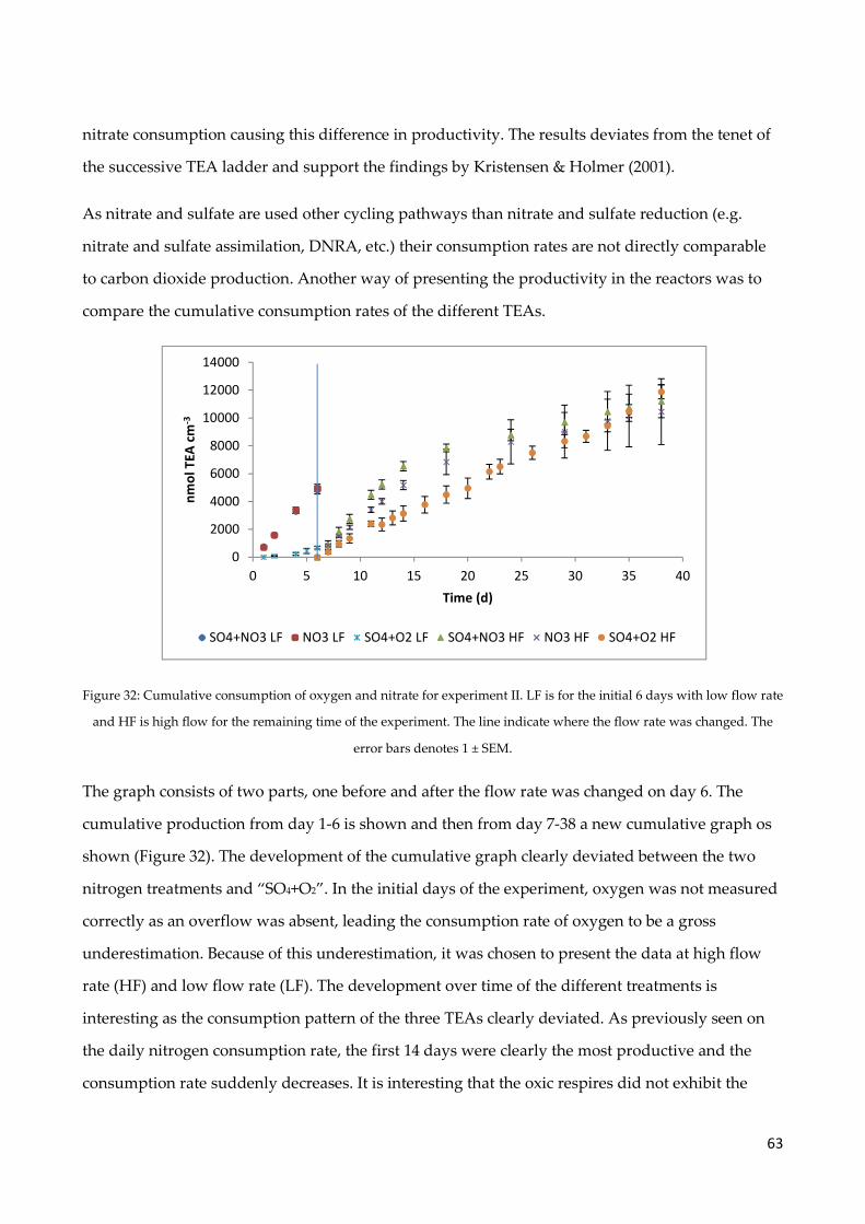
63
nitrate consumption causing this difference in productivity. The results deviates from the tenet of
the successive TEA ladder and support the findings by Kristensen & Holmer (2001).
As nitrate and sulfate are used other cycling pathways than nitrate and sulfate reduction (e.g.
nitrate and sulfate assimilation, DNRA, etc.) their consumption rates are not directly comparable
to carbon dioxide production. Another way of presenting the productivity in the reactors was to
compare the cumulative consumption rates of the different TEAs.
Figure 32: Cumulative consumption of oxygen and nitrate for experiment II. LF is for the initial 6 days with low flow rate
and HF is high flow for the remaining time of the experiment. The line indicate where the flow rate was changed. The
error bars denotes 1 ± SEM.
The graph consists of two parts, one before and after the flow rate was changed on day 6. The
cumulative production from day 1-6 is shown and then from day 7-38 a new cumulative graph os
shown (Figure 32). The development of the cumulative graph clearly deviated between the two
nitrogen treatments and “SO4+O2”. In the initial days of the experiment, oxygen was not measured
correctly as an overflow was absent, leading the consumption rate of oxygen to be a gross
underestimation. Because of this underestimation, it was chosen to present the data at high flow
rate (HF) and low flow rate (LF). The development over time of the different treatments is
interesting as the consumption pattern of the three TEAs clearly deviated. As previously seen on
the daily nitrogen consumption rate, the first 14 days were clearly the most productive and the
consumption rate suddenly decreases. It is interesting that the oxic respires did not exhibit the
0
2000
4000
6000
8000
10000
12000
14000
0 5 10 15 20 25 30 35 40
nm
ol
TE
A c
m-3
Time (d)
SO4+NO3 LF NO3 LF SO4+O2 LF SO4+NO3 HF NO3 HF SO4+O2 HF
64
same productivity as the nitrate treatments if a labile fraction was available. This may partly be
explained by poor measurements of oxygen at the start of the experiment. However, the daily
carbon dioxide production was also unaffected by the large consumption of the TEA. The reason
for the drop might therefore be due to immobilization, nitrate reduction or a combination of both.
Based on the cumulative graph for respectively carbon dioxide and TEA, the treatment “SO4+O2” is
thought to over time to display the highest rate of consumption of TEA. The reason for this
deviation is probably linked to the production of ROS which enhances the decomposition of
refractory organic matter (Canfield 1994). The difference between this treatment and the other is
probably not as great as Figure 29 suggested. Despite the unknown effect the oxic respiration had
on the dissolution of CaCO3, it is believed that oxygen was consumed to a higher extent than the
remaining treatments.
6. Conclusion
As described in multiple sections in the study the setup of the FTR experiment proved challenging.
The FTR experimental setup was for experiment I capable of identifying the labile fraction but
unfortunately, not for experiment II presumably because a portion of the labile fraction was
flushed and thereby lost before the start of the experiment. The experimental method enabled
precise and accurate measurement of the consumption rates of nitrate, oxygen, and production
rates of carbon dioxide. Sulfate might also be measureable if the supplied concentration is
decreased.
For future experiments, several conditions can be optimized some of which have been discussed in
the study. Addition of calcium bromide to the reservoir water is recommended for future
experiments. Bromide will function as an inert tracer for the break through experiment whilst
calcium will retard the dissolution of CaCO3. Calcium should still be monitored as the impact it
has had for this study and others (Pallud et al. 2007; Green & Aller 1998; Hulthe et al. 1998) were
large. The pH of the reservoirs and the samples should likewise be measured regularly. To
stabilize the pH it is recommended to use a buffer system. Some essentials minerals and nutrients
could possibly be added on low amounts to be ensure the decomposers are not nutrient/mineral
limited. If sulfate is to be measured by IC an improvement to the setup could be to decrease the

65
initial concentration of sulfate in the reservoirs to around 1-4 mM as done by Pallud et al. (2007) in
order to at least measure a relative change. The experimental setup is highly recommended, as it
provides a unique possibility to reflect day-to-day variation of decomposition rates of organic
matter in the sediment using various TEAs and enables the user to alteration of the flow and the
composition of inflow water relatively fast.
Innovative analytical methods of measuring ΣCO2 and sulfate in aqueous samples were developed
and employed in this study. The alternative method for measurement of carbon dioxide was based
on a gas sensor positioned in a jar in which carbon dioxide was measured in the gas phase. GSIre
compared to Gran titration proved capable of producing reliable result in the range of 0 – 5 mM
ΣCO2 and possible far beyond. The data points were precise and accurate and the method holds a
great potential and could easily be implemented in future experiments.
The second analytical method revolving precipitation of barium sulfate and fAAS proved to be
capable of measuring sulfate with a precision and accuracy that was unacceptable for the
consumption in the range, which the FTR generated in this experiment (Figure 23). When
measuring stock solution the method under- and overestimate the concentration of sulfate in the
samples. Further development is required to evaluate if this was correlated to poor measurements,
or if an unknown factor influences the measurement. If the method has a standard deviation of less
than 2% as indicated by one of the experiments (see Figure 8) this method holds a great potential
for experiments of sulfate. The possible number of samples analyzed on a day seem likely to be in
the three digit range. Further research is required if the analytical method is to be utilized in future
studies, but the author is of the opinion the method is useful and should not be discarded.
Due to incongruence between the consumption of TEA and production of carbon dioxide, a source
of non-biological carbon dioxide was sought. The dissolution of CaCO3 was found to contribute to
the ΣCO2 production. Samples at days before and after the flow rate was changed in experiment II
indicated the concentration of calcium differed at high and low flow rate. Based on both
measurements, the dissolution of CaCO3 from the sediment in the reactors was calculated to
contribute approximately 60% of the ΣCO2 from the reactors at both low and high flow rate. This
indicated the rate of dissolution was strongly dependent on the residence time and had, at least at
high flow rate, yet to obtain saturation. This finding is in accordance with Svensson & Dreybrodt

66
(1992) who found the time to reach equilibrium for the dissolution of CaCO3 was far longer than
the residence time in the reactor for this experiment.
The two FTR experiments displayed different patterns in their developments of the daily carbon
dioxide production rate with experiment I showing a greater decrease during the experiment
compared to experiment II. Freezing and subsequently thawing of the sediment used in
experiment II likely resulted in an initial leaching of the labile fraction of the sediment similar to
what Andersen (1996) and Kristensen & Holmer (2001) experienced in their studies. There was
visual evidence of this leaching but it was not verified through measurements. However, the data
obtained from the daily carbon dioxide production for the treatment “SO4-O2” was similar for
experiment I and II before the flow rate was changed. This indicate the sediment before and after
the freezing possible could contain a labile fraction of somewhat similar magnitude. The degree
and importance of which the sediment have been affected is therefore impossible to quantify.
Based on the consumption of nitrate at the end of experiment I and II, the limiting factor for the
anaerobic decomposition through various nitrogen pathways was suggested to be the hydrolysis
and not the energetically difference between TEA respiration reactions. This was in accordance
with other studies (Kristensen et al. 1995; Kristensen & Holmer 2001). It was interesting that the
decomposition rate of nitrate found in this study was so much lower than the rates listed in other
studies (Pallud et al., 2007; Laverman et al. 2012). The reason why this study was unable to obtain
similar rates could be correlated to a lower portion of labile matter being available simple due to a
difference in storage time.
It was interesting that the large consumption of nitrate occurring for the first 14 days in experiment
II did not result in greater production of carbon dioxide. As mentioned above, an unknown
portion of the labile fraction was lost due to freezing and it is unlikely that this could explain the
large consumption. This is supported by the findings of relative much lower consumptions of
oxygen in the same period. Alternatively, the nitrate may have been immobilized by the
decomposers at the beginning of the experiment (first 14 days), after which nitrate fell once the
decomposers were saturated with nitrogen.
67
The aerobic and anaerobic decomposition of salt marsh using a FTR experimental setup was for
experiment II carried out with success. In the initial phase, there did not seem to be any difference
in the aerobic and anaerobic treatments, but over the course of the experiment, the aerobic
treatment became the most productive based on the production of carbon dioxide and the
cumulative consumption of TEA (Figure 29 and Figure 32). This supported other findings
performed by (Kristensen & Holmer 2001; Kristensen et al. 1995) amongst others. There was no
statistically evidence for a difference between using nitrate and sulfate (SO4+NO3) or only nitrate
(NO3), but the RQ values indicated sulfate reduction might have occurred. As the concentrations
was similar to what is measured in the nature it seems plausible that the decomposition through
nitrate pathways occur simultaneously with sulfate reduction under these circumstances. There
was therefore experimental evidence in this study to support the idea that high levels of nitrate
from eutrophication would increase rates of salt marsh peat decomposition compared to anaerobic
(sulfate reduction) decomposition. The importance of the sulfate reduction has, however to be
investigated and further research is required.
68
7. Reference list
Andersen, F.O., 1996. Fate of organic carbon added as diatom cells to oxic and anoxic marine
sediment microcosms. Marine Ecology Progress Series, 134(1991), pp.225–233.
Anisfeld, S.C. & Hill, T.D., 2012. Fertilization Effects on Elevation Change and Belowground
Carbon Balance in a Long Island Sound Tidal Marsh. Estauries and Coasts, (35), pp.201–211.
Bethke, C.M. et al., 2011. The thermodynamic ladder in geomicrobiology. American Journal of
Science, 311, pp.183–210.
Burakham, R. et al., 2004. Flow injection spectrophotometry coupled with a crushed barium sulfate
reactor column for the determination of sulfate ion in water samples. Talanta, 64, pp.1147–
1150.
Canfield, D., Kristensen, E. & Thamdrup, B., 2005. Aquatic Geomicrobiology, Volume 48 (Advances in
Marine Biology) 1st ed., Elsevier.
Canfield, D.E., 1994. Factors influencing organic carbon preservation in marine sediments.
Chemical Geology, 2541(93), pp.315–329.
Chang, R., 2008. General Chemistry: The essential concepts 5th ed., McGraw-Hill.
Chou, L., Garrels, R.M. & Wallast, R., 1989. Comparative study of the kinetics and mechanisms of
dissolution of carbonate minerals. Chemical Geology, 78, pp.269–282.
Darby, F.A. & Turner, R.E., 2008. Effects of eutrophication on salt marsh root and rhizome biomass
accumulation. Marine Ecology Progress Series, 363, pp.63–70.
Deegan, L.A. et al., 2012. Coastal eutrophication as a driver of salt marsh loss. Nature, 490(7420),
pp.388–392. Available at: http://dx.doi.org/10.1038/nature11533.
Gomes, T.F. et al., 2014. Analytical Methods of sulfate in rainwater. Anal. Methods, 6, pp.4889–4894.
Gran, G., 1952. Determination of the Equivalence Point in Potentiometric Titrations. Part II. The
Analyst, pp.661–671.
69
Green, M.A. & Aller, R.C., 1998. Seasonal patterns of carbonate diagenesis in nearshore terrigenous
muds : Relation to spring phytoplankton bloom and temperature. Journal of Marine Research,
56, pp.1097–1123.
Hansen, L.S. & Blackburn, T.H., 1991. Aerobic and Anaerobic Mineralization of Organic Material
in Marine Sediment Microcosms. Marine Ecology Progress Series, 75(2-3), pp.283–291. Available
at:
http://gateway.webofknowledge.com/gateway/Gateway.cgi?GWVersion=2&SrcAuth=mekent
osj&SrcApp=Papers&DestLinkType=FullRecord&DestApp=WOS&KeyUT=A1991GG43500017
.
Hulthe, G., Hulth, S. & Hall, P.O.J., 1998. Effect of oxygen on degradation rate of refractory and
labile organic matter in continental margin sediments. Geochimica et Cosmochimica Acta, 62(8),
pp.1319–1328.
Jørgensen, B. & Sørensen, J., 1985. Seasonal cycles of 02, NO3-and SO,’-reduction in estuarine
sediments: the significance of an NO3 reduction in spring. Marine Ecology Progress Series, 24,
pp.65–74. Available at:
http://scholar.google.com/scholar?hl=en&btnG=Search&q=intitle:Seasonal+cycles+of+o2,no3+a
nd+so4+reduction+in+estuarine+sediments:+the+significance+of+an+no3+reduction+maximu
m+in+spring#3.
Kirwan, M.L. et al., 2010. Limits on the adaptability of coastal marshes to rising sea level.
Geophysical Research Letters, 37(23), pp.1–5. Available at:
http://doi.wiley.com/10.1029/2010GL045489.
Kristensen, E., 2000. Organic matter diagenesis at the oxic / anoxic interface in coastal marine
sediments, with emphasis on the role of burrowing animals. Hydrobiologia, 426, pp.1–24.
Kristensen, E., Ahmed, S.I. & Devol, A.H., 1995. Aerobic and anaerobic decomposition of organic
matter in marine sediment: Which is fastest ? American Society of Limnology and Oceanography,
40(8), pp.1430–1437. Available at: http://www.jstor.org/stable/2838498.
Kristensen, E. & Hansen, K., 1995. Decay of plant detritus in organic-poor marine sediment:

70
Production rates and stoichiometry C and N compounds marine sediment of dissolved C and
N compounds. Journal of Marine Research, 53, pp.675–702.
Kristensen, E. & Holmer, M., 2001. Decomposition of plant materials in marine sediment exposed
to different electron acceptors (O2, NO3 and SO4), with emphasis on substrate
origin,degradation kinetics, and the role of bioturbation. Geochimica et Cosmochimica Acta,
65(3), pp.419–433.
Krug, F.J., Filho, H.B. & Zagatto, E.A.G., 1977. Rapid Determination of Sulphate in Natural Waters
and Plant Digests by Continuous Flow Injection Turbidimetry. Analyst, 102, pp.503–508.
Laverman, A.M. et al., 2006. Potential rates and pathways of microbial nitrate reduction in coastal
sediments. FEMS Microbial Ecol, 58, pp.179–192.
Laverman, A.M., Abell, J. & Cappellen, P. Van, 2012. Comparative survey of potential nitrate and
sulfate reduction rates in aquatic sediments. Geochimica et Cosmochimica Acta, 77, pp.474–488.
Mann, K.., 2000. Salt marshes. In Ecology of Coastal Water With Implications for Management. John
Wiley & Sons, pp. 31–50.
Morais, P.A. et al., 2003. Use of a single air segment to minimise dispersion and improve mixing in
sequential injection : turbidimetric determination of sulphate in waters. Water Research, 37,
pp.4243–4249.
Morales, A., Graterol, L.S. De & Mesa, J., 2000. Determination of chloride, sulfate and nitrate in
groundwater samples by ion chromatography. Journal of Chromatography, 884, pp.185–190.
Morris, J.T., 1991. EFFECTS OF NITROGEN LOADING ON WETLAND ECOSYSTEMS WITH
PARTICULAR REFERENCE TO ATMOSPHERIC DEPOSITION. Ecol. Syst., 22, pp.257–279.
Morris, J.T. et al., 2002. Responses of Coastal Wetlands to Rising Sea Level. Ecology, 83(10),
pp.2869–2877. Available at: http://dx.doi.org/10.1890/0012-
9658(2002)083[2869:ROCWTR]2.0.CO;2.
Morris, J.T., Sundberg, K. & Hopkinson, C.S., 2013. Salt Marsh Primary Production and Its
Response to Relative Sea Level and Nutrients in Estuaries at Plum Island, Massachusets, and
71
North Inlet, South Carolina, USA. Oceanography, 26(3), pp.78–84.
Pallud, C. et al., 2007. The use of flow-through sediment reactors in biogeochemical kinetics:
Methodology and examples of applications. Marine Chemistry, 106(1-2), pp.256–271. Available
at: http://linkinghub.elsevier.com/retrieve/pii/S0304420306002179.
Pallud, C. & Van Cappellen, P., 2006. Kinetics of microbial sulfate reduction in estuarine
sediments. Geochimica et Cosmochimica Acta, 70(5), pp.1148–1162. Available at:
http://linkinghub.elsevier.com/retrieve/pii/S0016703705008495.
Presley, B.J., 1971. Techniques for analyzing interstitial water samples. Part 1 : Determination of
selected minor and major inorganic constituents. Initial Report. Institute of Geophysics &
Planetary Physics, 869, pp.1749–1755.
R.J Bertolacini, J.E.B., 1957. Colorimetric Determination of Sulfate with Barium Chloranilate. , 29(2),
pp.281–283.
Roy, A., Kanti, B. & Jayanta, D., 2011. Development and Validation of a Spectrophotometric
Method to Measure Sulfate Concentrations in Mine Water without Interference. Mine Water
Environ, 30, pp.169–174.
Roychoudhury, a. N., Viollier, E. & Van Cappellen, P., 1998. A plug flow-through reactor for
studying biogeochemical reactions in undisturbed aquatic sediments. Applied Geochemistry,
13(97), pp.269–280.
Seinfeld, J.H. & Pandis, S.N., 2006. Atmospheric Chemistry and Physics From Air Pollution to Climate
Change 2nd ed., John Wiley & Sons, Inc.
Stam, M.C. et al., 2011. 34S/32S fractionation by sulfate-reducing microbial communities in
estuarine sediments. Geochimica et Cosmochimica Acta, 75(14), pp.3903–3914. Available at:
http://linkinghub.elsevier.com/retrieve/pii/S0016703711002511.
Svensson, U. & Dreybrodt, W., 1992. Dissolution kinetics of natural calcite minerals in CO2-water
systems approaching calcite equilibrium. Chemical Geology, 100, pp.129–145.
Townend, I. et al., 2011. A review of salt marsh dynamics. Water and Environment Journal, 25(4),
72
pp.477–488. Available at: http://doi.wiley.com/10.1111/j.1747-6593.2010.00243.x.
Turner, R.E. et al., 2009. Salt marshes and eutrophication : An unsustainable outcome. Limnology
and Oceanography, 54(5), pp.1634–1642.
Valiela, I. et al., 1976. Production and dynamics of experimentally enriched salt marsh vegetation :
Belowground biomass. Limnology and Oceanography, 21(2), pp.245–252.
Valiela, I. & Cole, M.L., 2002. Comparative Evidence That Salt Marshes and Mangroves May
Protect Seagrass Meadows from Land-Derived Nitrogen Loads. Ecosystems, 5(1), pp.92–102.
Vernberg, F.J., 1993. Salt-marsh processes: A Review. Environmental Toxicology and Chemistry, 12,
pp.2167–2195. Available at: http://doi.wiley.com/10.1002/etc.5620121203.
Vernier, 2016. CO2 Gas Sensor. , pp.1–6. Available at: http://www.vernier.com/files/manuals/co2-
bta/co2-bta.pdf.
Westrich, J.T. & Berner, R. a., 1984. The role of sedimentary organic matter in bacterial sulfate
reduction: The G model tested. Limnology and Oceanography, 29(2), pp.236–249.