role of meteorology in seasonality of air pollution in megacity delhi, india

Role of meteorology in seasonality of air pollutionin megacity Delhi, India

Sarath K. Guttikunda & Bhola R. Gurjar

Received: 16 November 2010 /Accepted: 8 June 2011 /Published online: 29 June 2011# Springer Science+Business Media B.V. 2011

Abstract The winters in megacity Delhi are harsh,smoggy, foggy, and highly polluted. The pollutionlevels are approximately two to three times thosemonitored in the summer months, and the severity isfelt not only in the health department but also in thetransportation department, with regular delays atairport operations and series of minor and majoraccidents across the road corridors. The impacts feltacross the city are both manmade (due to the fuelburning) and natural (due to the meteorologicalsetting), and it is hard to distinguish their respectiveproportions. Over the last decade, the city has gainedfrom timely interventions to control pollution, andyet, the pollution levels are as bad as the previousyear, especially for the fine particulates, the mostharmful of the criteria pollutants, with a daily 2009average of 80 to 100 μg/m3. In this paper, the role ofmeteorology is studied using a Lagrangian modelcalled Atmospheric Transport Modeling System intracer mode to better understand the seasonality ofpollution in Delhi. A clear conclusion is that

irrespective of constant emissions over each month,the estimated tracer concentrations are invariably 40%to 80% higher in the winter months (November,December, and January) and 10% to 60% lower in thesummer months (May, June, and July), when com-pared to annual average for that year. Along withmonitoring and source apportionment studies, thispaper presents a way to communicate complexphysical characteristics of atmospheric modeling insimplistic manner and to further elaborate linkagesbetween local meteorology and pollution.

Keywords Air quality in Delhi . Particulatespollution .Winter highs .Mixing layer height . Role ofmeteorology

Introduction

Delhi, one of the largest megacities of South Asia andthe capital of India, is located at 28.5° N latitude and77° E longitude and 216 m above mean sea level.Delhi lies almost entirely on the Gangetic plains withthe Thar Desert in the West, central hot plains in theSouth, and hills in the North and East. The riverYamuna forms the eastern boundary passing throughthe city. The city lies in a semi-arid climate zone, withlong summers (early April to October), monsoonseason in between, and notorious winters (October toJanuary) with heavy fog (Ali et al. 2004). In the lasttwo decades, the city grew from being Delhi to

Environ Monit Assess (2012) 184:3199–3211DOI 10.1007/s10661-011-2182-8

S. K. Guttikunda (*)Division of Atmospheric Sciences,Desert Research Institute,2215 Raggio Parkway,Reno, NV 89512, USAe-mail: [email protected]

B. R. GurjarAssociate Professor, Department of Civil Engineering,Indian Institute of Technology, Roorkee,Roorkee 244667, India

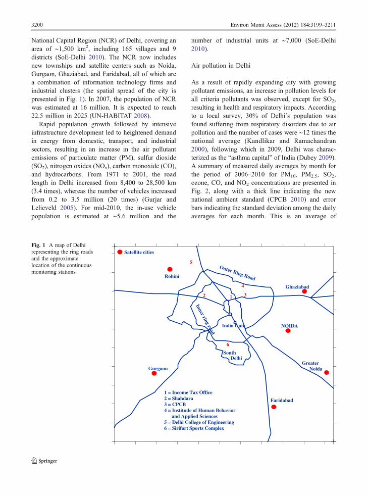
National Capital Region (NCR) of Delhi, covering anarea of ∼1,500 km2, including 165 villages and 9districts (SoE-Delhi 2010). The NCR now includesnew townships and satellite centers such as Noida,Gurgaon, Ghaziabad, and Faridabad, all of which area combination of information technology firms andindustrial clusters (the spatial spread of the city ispresented in Fig. 1). In 2007, the population of NCRwas estimated at 16 million. It is expected to reach22.5 million in 2025 (UN-HABITAT 2008).

Rapid population growth followed by intensiveinfrastructure development led to heightened demandin energy from domestic, transport, and industrialsectors, resulting in an increase in the air pollutantemissions of particulate matter (PM), sulfur dioxide(SO2), nitrogen oxides (NOx), carbon monoxide (CO),and hydrocarbons. From 1971 to 2001, the roadlength in Delhi increased from 8,400 to 28,500 km(3.4 times), whereas the number of vehicles increasedfrom 0.2 to 3.5 million (20 times) (Gurjar andLelieveld 2005). For mid-2010, the in-use vehiclepopulation is estimated at ∼5.6 million and the

number of industrial units at ∼7,000 (SoE-Delhi2010).

Air pollution in Delhi

As a result of rapidly expanding city with growingpollutant emissions, an increase in pollution levels forall criteria pollutants was observed, except for SO2,resulting in health and respiratory impacts. Accordingto a local survey, 30% of Delhi’s population wasfound suffering from respiratory disorders due to airpollution and the number of cases were ∼12 times thenational average (Kandlikar and Ramachandran2000), following which in 2009, Delhi was charac-terized as the “asthma capital” of India (Dubey 2009).A summary of measured daily averages by month forthe period of 2006–2010 for PM10, PM2.5, SO2,ozone, CO, and NO2 concentrations are presented inFig. 2, along with a thick line indicating the newnational ambient standard (CPCB 2010) and errorbars indicating the standard deviation among the dailyaverages for each month. This is an average of

Rohini

Gurgaon

Faridabad

GreaterNoida

NOIDA

Ghaziabad

Outer Ring Road

Inner ring road

SouthDelhi

Satellite cities

1 32

5

4

6

India Gate

1 = Income Tax Office2 = Shahdara3 = CPCB4 = Institude of Human Behavior and Applied Sciences5 = Delhi College of Engineering6 = Sirifort Sports Complex

Fig. 1 A map of Delhirepresenting the ring roadsand the approximatelocation of the continuousmonitoring stations

3200 Environ Monit Assess (2012) 184:3199–3211

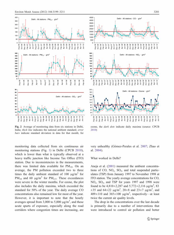
monitoring data collected from six continuous airmonitoring stations (Fig. 1) in Delhi (CPCB 2010),which is lower than what is typically observed at aheavy traffic junction like Income Tax Office (ITO)station. Due to inconsistencies in the measurements,there was limited data available for PM10. On anaverage, the PM pollution exceeded two to threetimes the daily ambient standard of 100 μg/m3 forPM10 and 60 μg/m3 for PM2.5. These exceedanceswere severe in the winter months. For ozone, the plotalso includes the daily maxima, which exceeded thestandard for 50% of the year. The daily average COconcentrations also remained low for most of the year.However, it is important to note that the hourlyaverages spread from 3,000 to 5,000 μg/m3, and theseacute spurts of exposure, especially along the roadcorridors where congestion times are increasing, are

very unhealthy (Gómez-Perales et al. 2007; Zhao etal. 2004).

What worked in Delhi?

Aneja et al. (2001) measured the ambient concentra-tions of CO, NOx, SO2, and total suspended partic-ulates (TSP) from January 1997 to November 1998 atITO station. The yearly average concentrations for CO,NOx, SO2, and TSP for years 1997 and 1998 werefound to be 4,810±2,287 and 5,772±2,116 μg/m3, 83±35 and 64±22 μg/m3, 20±8 and 23±7 μg/m3, and409±110 and 365±100 μg/m3, respectively—at leasttwice the current air quality levels.

The drop in the concentrations over the last decadeis primarily due to a number of interventions thatwere introduced to control air pollution and better

Delhi - All stations - PM2.5 - µg/m3

0

60

120

180

240

300

360

420A

ug

-06

Oc

t-06

De

c-0

6

Feb

-07

Ap

r-07

Jun-

07

Au

g-0

7

Oc

t-07

De

c-0

7

Feb

-08

Ap

r-08

Jun-

08

Au

g-0

8

Oc

t-08

De

c-0

8

Feb

-09

Ap

r-09

Jun-

09

Au

g-0

9

Oc

t-09

De

c-0

9

Feb

-10

Ap

r-10

Jun-

10

Delhi - All stations - CO -µg/m3

0

500

1000

1500

2000

2500

3000

3500

4000

4500

Au

g-0

6

Oc

t-06

De

c-0

6

Feb

-07

Ap

r-07

Jun-

07

Au

g-0

7

Oc

t-07

De

c-0

7

Feb

-08

Ap

r-08

Jun-

08

Au

g-0

8

Oc

t-08

De

c-0

8

Feb

-09

Ap

r-09

Jun-

09

Au

g-0

9

Oc

t-09

De

c-0

9

Feb

-10

Ap

r-10

Jun-

10

Delhi - All stations - PM10 - µg/m3

0

50

100

150

200

250

300

350

400

450

500

Au

g-0

6

Oc

t-06

De

c-0

6

Feb

-07

Ap

r-07

Jun-

07

Au

g-0

7

Oc

t-07

De

c-0

7

Feb

-08

Ap

r-08

Jun-

08

Au

g-0

8

Oc

t-08

De

c-0

8

Feb

-09

Delhi - All stations - NO2 - µg/m3

0

20

40

60

80

100

120

140

160

180

200

Au

g-0

6

Oc

t-06

De

c-0

6

Feb

-07

Ap

r-07

Jun-

07

Au

g-0

7

Oc

t-07

De

c-0

7

Feb

-08

Ap

r-08

Jun-

08

Au

g-0

8

Oc

t-08

De

c-0

8

Feb

-09

Ap

r-09

Jun-

09

Au

g-0

9

Oc

t-09

De

c-0

9

Feb

-10

Ap

r-10

Jun-

10

Delhi - All stations - SO2 - µg/m3

0

10

20

30

40

50

60

70

80

90

Au

g-0

6

Oc

t-06

De

c-0

6

Feb

-07

Ap

r-07

Jun-

07

Au

g-0

7

Oc

t-07

De

c-0

7

Feb

-08

Ap

r-08

Jun-

08

Au

g-0

8

Oc

t-08

De

c-0

8

Feb

-09

Ap

r-09

Jun-

09

Au

g-0

9

Oc

t-09

De

c-0

9

Feb

-10

Ap

r-10

Jun-

10

Delhi - All stations - Ozone -µg/m3

0

20

40

60

80

100

120

140

160

180

200

Au

g-0

6

Oc

t-06

De

c-0

6

Feb

-07

Ap

r-07

Jun-

07

Au

g-0

7

Oc

t-07

De

c-0

7

Feb

-08

Ap

r-08

Jun-

08

Au

g-0

8

Oc

t-08

De

c-0

8

Feb

-09

Ap

r-09

Jun-

09

Au

g-0

9

Oc

t-09

De

c-0

9

Feb

-10

Ap

r-10

Jun-

10

Fig. 2 Average of monitoring data from six stations in Delhi,India; thick line indicates the national ambient standard; errorbars indicate standard deviation in data for that month; for

ozone, the dark dots indicate daily maxima (source: CPCB2010)

Environ Monit Assess (2012) 184:3199–3211 3201

urban planning by the local government. In 1998, theSupreme Court ruled that the city of Delhi should takeconcrete steps to address air pollution in the transportand industrial sectors. The timeline of implementation(in the transport and industrial sector) and theexperience for instituting change which has becomea model for other Indian cities is described in detail inNarain and Bell (2005). For the transport sector, thisruling led to largest ever compressed natural gas(CNG) switch in the world for public transportvehicles. More than 100,000 vehicles (including thethree wheelers and taxis) were converted to CNG overfive years (DTC 2010). This resulted in significantdecrease in the PM pollution—largest improvementcame from retrofitting ∼3,000 diesel buses to CNG(DTE 2002). Kandlikar (2007) attributes the follow-ing changes to the introduction of CNG: a dramaticdrop of 40% in the CO concentrations for the calendaryear 2002 from 5,000 to 3,000 μg/m3 and the NOx

concentrations showed an increase of 50% from 63 to95 μg/m3 from January 2001 to January 2004followed by a slow decrease to 82 μg/m3 by January2006. Kandlikar (2007) concludes that the reversetrend in NOx concentrations is linked more to therapid changes in the vehicle fleet, which quicklynegated the benefits of CNG conversion. The con-centration of SO2 showed a decline of about 33%,from 15 to 10 μg/m3, which is a result of theconversion to CNG and reduction in diesel fuel sulfurcontent introduced in 2001–2002 (Badami 2005).Delhi has, since 2000, also enforced Euro II emissionstandards, 5 years ahead of schedule, Euro III in 2005for all passenger vehicles, and Euro IV fuel standardsin April 2010 (in Delhi and 11 other cities).

Other significant fallout of the ruling was in theindustrial sector—approximately 500 heavy industrieswere either shut down or relocated to areas outside theDelhi administrative boundaries, which the industriestook the opportunity to upgrade (while relocating)their energy systems to improve energy efficiency andconsumption levels.

Yet, there remains a tremendous amount of potentialto reduce the air pollution impacts in Delhi as thedemand rises for infrastructure and services. Reynoldsand Kandlikar (2008) examined the opportunities forcombined benefits of Delhi’s fuel switching strategy—not only for local air pollution but also for climate-related affects—and evaluated the potential for extend-ing such services to other cities.

Scope of this paper

While there is no single sector that is solely responsiblefor Delhi’s air pollution, rather a combination of sourcesincluding industries, power plants, domestic combus-tion of coal and biomass, and transport (direct vehicleexhaust and indirect road dust) contribute to airpollution (CPCB 2010; Chowdhury et al. 2007; Mohanand Kandya 2007; Garg et al. 2006; Gurjar et al. 2004;Reddy and Venkataraman 2002; Shah et al. 2000),though the sectoral contributions vary considerablyfrom season to season. Seasonal changes in demandfor fuel and natural pollution result in differing sourcecontributions during the summer and the wintermonths. This needs further evaluation for not onlythe emission trends but also the changing meteorolog-ical conditions from season to season in order tomaximize the effectiveness of anti-pollution initiatives(Guttikunda 2009; Gurjar et al. 2004, 2008; Mohanand Kandya 2007).

It is generally believed that the air pollution canonly be controlled at the source, and the limitingfactor is most often the balance sheet of costs andassociated benefits (like health). However, in somecases, possible reduction in emissions is a directfunction of the geographical location and prevalentmeteorological conditions. For example, in cities likeLos Angeles or Ulaanbaatar, which form a valleyterrain, irrespective of the wind patterns, the emis-sions tend to stay in the area longer and contributemore to the local air pollution problems. On the otherhand, in cities like Bangkok, Beijing, Delhi, Dhaka,and Manila, with flat terrains, the meteorology tendsto have higher impact on dispersing the air pollution.In this regards, a study of air movement over urbanareas can help us better understand the movement ofpollutants and their respective impact on pollutionplanning. In this paper, in combination with monitor-ing data from the Pollution Control Board andparticulate pollution source apportionment analysisin the literature, we assess the role of meteorology forthe period of 2000s as a diffusing or non-diffusingagent of air pollution in megacity Delhi, India.

Study methodology

The fundamental parameter in the movement ofcontaminants is the wind, its speed and direction,


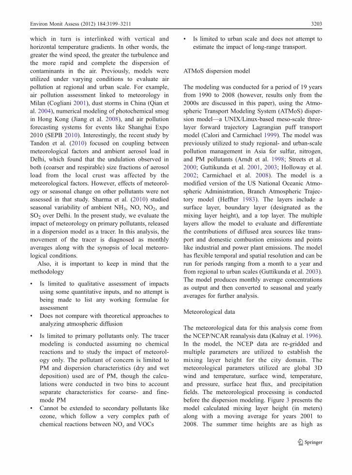
which in turn is interlinked with vertical andhorizontal temperature gradients. In other words, thegreater the wind speed, the greater the turbulence andthe more rapid and complete the dispersion ofcontaminants in the air. Previously, models wereutilized under varying conditions to evaluate airpollution at regional and urban scale. For example,air pollution assessment linked to meteorology inMilan (Cogliani 2001), dust storms in China (Qian etal. 2004), numerical modeling of photochemical smogin Hong Kong (Jiang et al. 2008), and air pollutionforecasting systems for events like Shanghai Expo2010 (SEPB 2010). Interestingly, the recent study byTandon et al. (2010) focused on coupling betweenmeteorological factors and ambient aerosol load inDelhi, which found that the undulation observed inboth (coarser and respirable) size fractions of aerosolload from the local crust was affected by themeteorological factors. However, effects of meteorol-ogy or seasonal change on other pollutants were notassessed in that study. Sharma et al. (2010) studiedseasonal variability of ambient NH3, NO, NO2, andSO2 over Delhi. In the present study, we evaluate theimpact of meteorology on primary pollutants, releasedin a dispersion model as a tracer. In this analysis, themovement of the tracer is diagnosed as monthlyaverages along with the synopsis of local meteoro-logical conditions.

Also, it is important to keep in mind that themethodology

& Is limited to qualitative assessment of impactsusing some quantitative inputs, and no attempt isbeing made to list any working formulae forassessment

& Does not compare with theoretical approaches toanalyzing atmospheric diffusion

& Is limited to primary pollutants only. The tracermodeling is conducted assuming no chemicalreactions and to study the impact of meteorol-ogy only. The pollutant of concern is limited toPM and dispersion characteristics (dry and wetdeposition) used are of PM, though the calcu-lations were conducted in two bins to accountseparate characteristics for coarse- and fine-mode PM

& Cannot be extended to secondary pollutants likeozone, which follow a very complex path ofchemical reactions between NOx and VOCs

& Is limited to urban scale and does not attempt toestimate the impact of long-range transport.

ATMoS dispersion model

The modeling was conducted for a period of 19 yearsfrom 1990 to 2008 (however, results only from the2000s are discussed in this paper), using the Atmo-spheric Transport Modeling System (ATMoS) disper-sion model—a UNIX/Linux-based meso-scale three-layer forward trajectory Lagrangian puff transportmodel (Calori and Carmichael 1999). The model waspreviously utilized to study regional- and urban-scalepollution management in Asia for sulfur, nitrogen,and PM pollutants (Arndt et al. 1998; Streets et al.2000; Guttikunda et al. 2001, 2003; Holloway et al.2002; Carmichael et al. 2008). The model is amodified version of the US National Oceanic Atmo-spheric Administration, Branch Atmospheric Trajec-tory model (Heffter 1983). The layers include asurface layer, boundary layer (designated as themixing layer height), and a top layer. The multiplelayers allow the model to evaluate and differentiatethe contributions of diffused area sources like trans-port and domestic combustion emissions and pointslike industrial and power plant emissions. The modelhas flexible temporal and spatial resolution and can berun for periods ranging from a month to a year andfrom regional to urban scales (Guttikunda et al. 2003).The model produces monthly average concentrationsas output and then converted to seasonal and yearlyaverages for further analysis.

Meteorological data

The meteorological data for this analysis come fromthe NCEP/NCAR reanalysis data (Kalnay et al. 1996).In the model, the NCEP data are re-gridded andmultiple parameters are utilized to establish themixing layer height for the city domain. Themeteorological parameters utilized are global 3Dwind and temperature, surface wind, temperature,and pressure, surface heat flux, and precipitationfields. The meteorological processing is conductedbefore the dispersion modeling. Figure 3 presents themodel calculated mixing layer height (in meters)along with a moving average for years 2001 to2008. The summer time heights are as high as


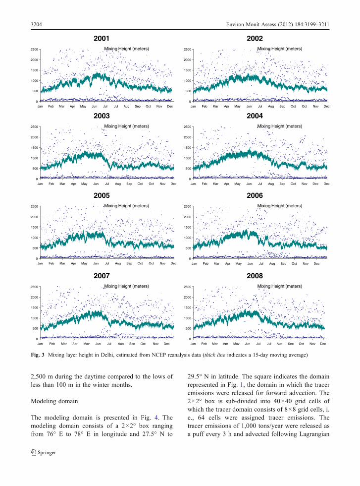
2,500 m during the daytime compared to the lows ofless than 100 m in the winter months.

Modeling domain

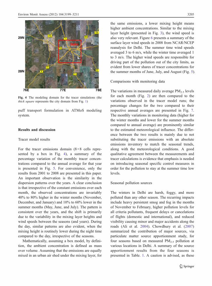
The modeling domain is presented in Fig. 4. Themodeling domain consists of a 2×2° box rangingfrom 76° E to 78° E in longitude and 27.5° N to

29.5° N in latitude. The square indicates the domainrepresented in Fig. 1, the domain in which the traceremissions were released for forward advection. The2×2° box is sub-divided into 40×40 grid cells ofwhich the tracer domain consists of 8×8 grid cells, i.e., 64 cells were assigned tracer emissions. Thetracer emissions of 1,000 tons/year were released asa puff every 3 h and advected following Lagrangian

2001Mixing Height (meters)

0

500

1000

1500

2000

2500

Jan Feb Mar Apr May Jun Jul Jul Aug Sep Oct Nov Dec


0

500

1000

1500

2000

2500

Jan Feb Mar Apr May Jun Jul Aug Sep Oct Oct Nov Dec


0

500

1000

1500

2000

2500




0

500

1000

1500

2000

2500

Jan Feb Mar Apr May Jun Jul Aug Sep Oct Nov Dec Dec

Jan Feb Mar Apr May Jun Jul Aug Sep Oct Nov Dec



0

500

1000

1500

2000

2500


0

500

1000

1500

2000

2500


0

500

1000

1500

2000

2500


0

500

1000

1500

2000

2500

Jan Feb Mar Apr May Jun Jul Jul Aug Sep Oct Nov Dec

Fig. 3 Mixing layer height in Delhi, estimated from NCEP reanalysis data (thick line indicates a 15-day moving average)


puff transport formulation in ATMoS modelingsystem.

Results and discussion

Tracer model results

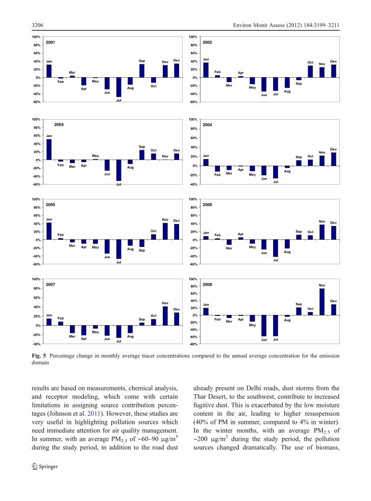
For the tracer emissions domain (8×8 cells repre-sented by a box in Fig. 4), a summary of thepercentage variation of the monthly tracer concen-trations compared to the annual average for that yearis presented in Fig. 5. For convenience, only theresults from 2001 to 2008 are presented in this paper.An important observation is the similarity in thedispersion patterns over the years. A clear conclusionis that irrespective of the constant emissions over eachmonth, the observed concentrations are invariably40% to 80% higher in the winter months (November,December, and January) and 10% to 60% lower in thesummer months (May, June, and July). The pattern isconsistent over the years, and the shift is primarilydue to the variability in the mixing layer heights andwind speeds between the seasons (and years). Duringthe day, similar patterns are also evident, when themixing height is routinely lower during the night timecompared to the day, irrespective of the seasons.

Mathematically, assuming a box model, by defini-tion, the ambient concentration is defined as massover volume. Assuming that the emissions are equallymixed in an urban air shed under the mixing layer, for

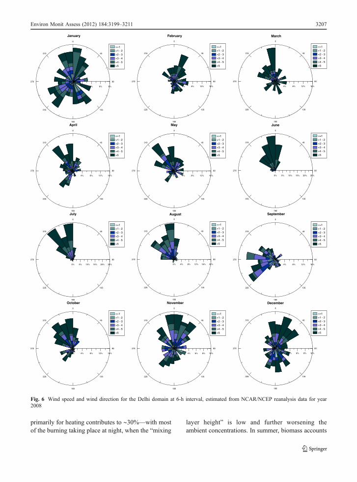
the same emissions, a lower mixing height meanshigher ambient concentrations. Similar to the mixinglayer height (presented in Fig. 3), the wind speed isalso very relevant. Figure 6 presents a summary of thesurface layer wind speeds in 2008 from NCAR/NCEPreanalysis for Delhi. The summer time wind speedsaveraged 3 to 6 m/s, while the winter time averaged 1to 3 m/s. The higher wind speeds are responsible fordriving part of the pollution out of the city limits, asevident from lower shares of tracer concentrations forthe summer months of June, July, and August (Fig. 5).

Comparisons with monitoring data

The variations in measured daily average PM2.5 levelsfor each month (Fig. 2) are then compared to thevariations observed in the tracer model runs; thepercentage changes for the two compared to theirrespective annual averages are presented in Fig. 7.The monthly variations in monitoring data (higher forthe winter months and lower for the summer monthscompared to annual average) are prominently similarto the estimated meteorological influence. The differ-ence between the two results is mainly due to notsubstituting the tracer emissions with an absoluteemissions inventory to match the seasonal trends,along with the meteorological conditions. A goodqualitative agreement between the measurements andtracer calculations is evidence that emphasis is neededon introducing seasonal specific control measures inorder for the pollution to stay at the summer time lowlevels.

Seasonal pollution sources

The winters in Delhi are harsh, foggy, and morepolluted than any other season. The recurring impactsinclude heavy persistent smog and fog in the monthsof November to February, higher pollution levels forall criteria pollutants, frequent delays or cancelationsof flights (domestic and international), and reducedvisibility causing minor and major accidents along theroads (Ali et al. 2004). Chowdhury et al. (2007)summarized the contribution of major sources, viaparticulate matter source apportionment study, forfour seasons based on measured PM2.5 pollution atvarious locations in Delhi. A summary of the sourceapportionment results from the four seasons ispresented in Table. 1. A caution is advised, as these

76E 78E

28N

29N

Delhi

77E

Fig. 4 The modeling domain for the tracer simulations (thethick square represents the city domain from Fig. 1)


results are based on measurements, chemical analysis,and receptor modeling, which come with certainlimitations in assigning source contribution percen-tages (Johnson et al. 2011). However, these studies arevery useful in highlighting pollution sources whichneed immediate attention for air quality management.In summer, with an average PM2.5 of ∼60–90 μg/m3

during the study period, in addition to the road dust

already present on Delhi roads, dust storms from theThar Desert, to the southwest, contribute to increasedfugitive dust. This is exacerbated by the low moisturecontent in the air, leading to higher resuspension(40% of PM in summer, compared to 4% in winter).In the winter months, with an average PM2.5 of∼200 μg/m3 during the study period, the pollutionsources changed dramatically. The use of biomass,

2001

Jan

Feb

Mar

Apr

May

Jun

Jul

Aug

Sep

Oct

Nov Dec

-60%

-40%

-20%

0%

20%

40%

60%

80%

100%

2002

Jan

Feb

Mar

Apr

May

Jun JulAug

Sep

Oct NovDec

-60%

-40%

-20%

0%

20%

40%

60%

80%

100%

2003

Jan

Feb Mar Apr

May

Jun

Jul

Aug

SepOct

Nov

Dec

-60%

-40%

-20%

0%

20%

40%

60%

80%

100%

2004

Jan

Feb MarApr

MayJun

Jul

Aug

Sep OctNov

Dec

-40%

-20%

0%

20%

40%

60%

80%

100%

2005

Jan

Feb

Mar Apr May

Jun

Jul

Aug Sep

Oct

Nov Dec

-60%

-40%

-20%

0%

20%

40%

60%

80%

100%

2006

JanFeb

Mar

Apr

May

Jun

Jul

Aug

Sep Oct

Nov Dec

-60%

-40%

-20%

0%

20%

40%

60%

80%

100%

2007

JanFeb

MarApr

May

JunJul

Aug

SepOct

Nov

Dec

-40%

-20%

0%

20%

40%

60%

80%

100%

2008

Jan

FebMar

Apr

May

Jun Jul

Aug

SepOct

Nov

Dec

-80%

-60%

-40%

-20%

0%

20%

40%

60%

80%

100%

Fig. 5 Percentage change in monthly average tracer concentrations compared to the annual average concentration for the emissiondomain


primarily for heating contributes to ∼30%—with mostof the burning taking place at night, when the “mixing

layer height” is low and further worsening theambient concentrations. In summer, biomass accounts

0

45

90

135

180

225

270

315

0% 2% 4% 6% 8%

<=1>1 - 2>2 - 3>3 - 4>4 - 5>5

January0

45

90

135

180

225

270

315

0% 4% 8% 12% 16%

<=1>1 - 2>2 - 3>3 - 4>4 - 5>5

February0

45

90

135

180

225

270

315

0% 4% 8% 12% 16%

<=1>1 - 2>2 - 3>3 - 4>4 - 5>5

March

0

45

90

135

180

225

270

315

0% 4% 8% 12% 16%

<=1>1 - 2>2 - 3>3 - 4>4 - 5>5

April

0

45

90

135

180

225

270

315

0% 4% 8% 12% 16%

<=1>1 - 2>2 - 3>3 - 4>4 - 5>5

May

0

45

90

135

180

225

270

315

0% 5% 10% 15% 20% 25%

<=1>1 - 2>2 - 3>3 - 4>4 - 5>5

June

0

45

90

135

180

225

270

315

0% 5% 10% 15% 20% 25%

<=1>1 - 2>2 - 3>3 - 4>4 - 5>5

July0

45

90

135

180

225

270

315

0% 4% 8% 12% 16% 20%

<=1>1 - 2>2 - 3>3 - 4>4 - 5>5

August0

45

90

135

180

225

270

315

0% 4% 8% 12% 16%

<=1>1 - 2>2 - 3>3 - 4>4 - 5>5

September

0

45

90

135

180

225

270

315

0% 4% 8% 12% 16%

<=1>1 - 2>2 - 3>3 - 4>4 - 5>5

October0

45

90

135

180

225

270

315

0% 2% 4% 6% 8% 10%

<=1>1 - 2>2 - 3>3 - 4>4 - 5>5

November0

45

90

135

180

225

270

315

0% 2% 4% 6% 8% 10%

<=1>1 - 2>2 - 3>3 - 4>4 - 5>5

December

Fig. 6 Wind speed and wind direction for the Delhi domain at 6-h interval, estimated from NCAR/NCEP reanalysis data for year2008


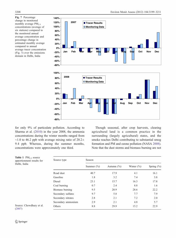
for only 9% of particulate pollution. According toSharma et al. (2010) in the year 2008, the ammoniaconcentrations during the winter months ranged from∼1.0 to 46.2 ppb with average mixing ratio of 20.2±9.4 ppb. Whereas, during the summer months,concentrations were approximately one third.

Though seasonal, after crop harvests, clearingagricultural land is a common practice in thesurrounding (largely agricultural) states, and thesmoke reaches Delhi contributing to substantial smogformation and PM and ozone pollution (NASA 2008).Note that the dust storms and biomass burning are not

2007

-80%

-60%

-40%

-20%

0%

20%

40%

60%

80%

100%

120%

140%


Tracer Results

Monitoring Data

2008

-80%

-60%

-40%

-20%

0%

20%

40%

60%

80%

100%


Tracer Results

Monitoring Data

Fig. 7 Percentagechange in monitoredmonthly average PM2.5

concentrations (average ofsix stations) compared tothe monitored annualaverage concentration andpercentage change inestimated monthly averagecompared to annualaverage tracer concentration(Fig. 5) over the emissionsdomain in Delhi, India

Source type Season

Summer (%) Autumn (%) Winter (%) Spring (%)

Road dust 40.7 17.9 4.1 16.1

Gasoline 1.8 3.2 7.4 3.8

Diesel 23.1 15.7 16.3 17.8

Coal burning 0.7 2.4 8.8 1.6

Biomass burning 9.5 20.9 28.6 22.2

Secondary sulfates 9.7 5.8 7.7 7.9

Secondary nitrates 2.8 2.1 7.2 2.0

Secondary ammonium 2.9 2.1 4.8 5.7

Others 8.8 29.9 15.2 22.9

Table 1 PM2.5 sourceapportionment results forDelhi, India

Source: Chowdhury et al.(2007)


necessarily natural phenomena. Desert crusts andvegetation can be destroyed via construction activitiesin the cities, thereby creating a reservoir of suspend-ible dust during high winds. These with anthropogen-ic activities compound the impact of what mightotherwise be viewed as purely natural phenomena,and they may change the importance of thesepollution sources within the context of an air qualitymanagement program. The dust events or the fires canonly be predicted using satellite and modeling databut cannot be prevented. However, the dust from thestorms or the smoke from forest fires can be detectedin advance and provide public pollution alerts basedon the meteorological tracer or chemical transportmodeling in forecast mode.

Conclusion

It is important to note that while the modeling isconducted using the meteorology pertinent to the cityarea, the tracer emissions are not. While the simu-lations provided a better understanding of the disper-sion and seasonality of air pollution in the city, thepollution patterns are best studied using a localemissions inventory, including the contributions ofemissions originating outside the city (transboundarypollution). For example, in case of Delhi, a constanttraffic between Delhi and its satellite cities (Gurgaonand NOIDA) is a growing emission source, alongwith all the industrial estates in the northeast andnorthwest sectors.

Studying the role of meteorology is crucial alsofrom mega event management perspective. Forexample, air pollution in Beijing received signifi-cant attention in 2008 before (and after) the 2008Olympic Games (Streets et al. 2007). A number ofinterventions were implemented in domestic, indus-trial, and transport sectors to achieve the target airpollution reductions and improve the number ofclean air (blue sky) days in Beijing (UNEP 2009).During the Olympic Games, the traffic was restrictedto only 50% of the passenger vehicles (depending onthe registration number) every day. And at theindustrial level, a number of small and large scaleunits were shut down. Most importantly, a number ofindustries were also shut down in the neighboringcities to cut down the long-range transport (due to

meteorological advection) of pollutants. With theinterventions in place, the levels of NOx (primarilyfrom the cars, trucks, and power plants) plunged∼50%. Likewise, levels of PM fell ∼20% (UNEP2009). Similar steps, with lesser intensity, wereimplemented in Delhi during the 2010 Common-wealth Games in October 2010, such as separatelanes for public and athletes, closing down of coal-based power plant in the city, and varying theworking hours of public offices to avoid somecongestion on the roads.

The linkages between pollutant emissions, meteorol-ogy, and health impacts are complex, and to formulatean integrated multi-pollutant strategy, one needs betterunderstanding of these linkages (Hidy and Pennell2010). For air quality management in Delhi and inother cities of India, the proposed methodology tostudy the movement of local emissions and the role ofmeteorology in either advecting or trapping thepollution in the city, along with any top-down sourceapportionment study like Chowdhury et al. (2007), canplay a vital role in communicating complex physicalcharacteristics of atmospheric modeling in simplisticmanner—and to further elaborate pollution parametersand potential health risks.

Acknowledgments This paper has not been subjected forinternal peer and policy review of the Indian agencies andtherefore does not necessarily reflect their views. The analysisand views expressed in this report are entirely those of theauthors. No official endorsement should be inferred. Secondauthor acknowledges support received from the Max PlanckSociety, Munich, and the Max Planck Institute for Chemistry,Mainz, Germany, through the Max Planck Partner Group forMegacities and Global Change established at Indian Institute ofTechnology Roorkee, India.

References

Ali, K., Momin, G. A., Tiwari, S., Safai, P. D., Chate, D. M., &Rao, P. S. P. (2004). Fog and precipitation chemistry atDelhi, North India. Atmospheric Environment, 38, 4215–4222.

Aneja, V. P., Agarwal, A., Roelle, P. A., Phillips, S. B., Tong, Q.,Watkins, N., et al. (2001). Measurements and analysis ofcriteria pollutants in New Delhi, India. EnvironmentInternational, 27, 35–42.

Arndt, R. L., Carmichael, G. R., & Roorda, J. M. (1998).Seasonal source–receptor relationships in Asia. Atmo-spheric Environment, 32, 1397–1406.


Badami, M. G. (2005). Transport and urban air pollution inIndia. Environmental Management, 36, 195–204.

Calori, G., & Carmichael, G. R. (1999). An urban trajectorymodel for sulfur in Asian megacities: model concepts andpreliminary application. Atmospheric Environment, 33,3109–3117.

Carmichael, G. R., Sakurai, T., Streets, D., Hozumi, Y., Ueda,H., Park, S. U., et al. (2008). MICS-Asia II: the modelintercomparison study for Asia Phase II methodology andoverview of findings. Atmospheric Environment, 42,3468–3490.

Chowdhury, Z., Zheng, M., Schauer, J. J., Sheesley, R. J.,Salmon, L. G., Cass, G. R., et al. (2007). Speciation ofambient fine organic carbon particles and source appor-tionment of PM2.5 in Indian cities. Journal of GeophysicalResearch, 112, D15303.

Cogliani, E. (2001). Air pollution forecast in cities by an airpollution index highly correlated with meteorologicalvariables. Atmospheric Environment, 35, 2871–2877.

CPCB. (2010). Central Pollution Control Board. New Delhi:Government of India.

DTC. (2010). Largest CNG-based fleet in the world. NewDelhi: Delhi Transport Corporation.

DTE. (2002). The Supreme Court not to budge on CNG issue.New Delhi: Down to Earth Magazine.

Dubey, M. (2009). Delhi is India’s Asthma capital. New Delhi:Mail Today. March 1, 2009.

Garg, A., Shukla, P. R., & Kapshe, M. (2006). The sectoraltrends of multigas emissions inventory of India. Atmo-spheric Environment, 40, 4608–4620.

Gómez-Perales, J. E., Colvile, R. N., Fernández-Bremauntz,A. A., Gutiérrez-Avedoy, V., Páramo-Figueroa, V. H.,Blanco-Jiménez, S., et al. (2007). Bus, minibus, metrointer-comparison of commuters’ exposure to air pollu-tion in Mexico City. Atmospheric Environment, 41, 890–901.

Gurjar, B. R., & Lelieveld, J. (2005). New directions:megacities and global change. Atmospheric Environment,39, 391–393.

Gurjar, B. R., van Aardenne, J. A., Lelieveld, J., & Mohan, M.(2004). Emission estimates and trends (1990–2000) formegacity Delhi and implications. Atmospheric Environ-ment, 38, 5663–5681.

Gurjar, B. R., Butler, T. M., Lawrence, M. G., & Lelieveld, J.(2008). Evaluation of emissions and air quality inmegacities. Atmospheric Environment, 42, 1593–1606.

Guttikunda, S.K. (2009). Air quality management in Delhi,India: Then, now, and next. In: UrbanEmissions.Info (Ed.),SIM-air Working Paper Series, 22–2009, New Delhi,India.

Guttikunda, S. K., Thongboonchoo, N., Arndt, R. L., Calori,G., Carmichael, G. R., & Streets, D. G. (2001). Sulfurdeposition in Asia: seasonal behavior and contributionsfrom various energy sectors. Water Air and Soil Pollution,131, 383–406.

Guttikunda, S. K., Carmichael, G. R., Calori, G., Eck, C., &Woo, J.-H. (2003). The contribution of megacities toregional sulfur pollution in Asia. Atmospheric Environ-ment, 37, 11–22.

Heffter, J.L. (1983). Branching atmospheric trajectory (BAT)model, NOAATech. Memo. ERL ARL-121, Air ResourcesLaboratory, Rockville, MD USA.

Hidy, G. M., & Pennell, W. T. (2010). Multipollutant air qualitymanagement. Journal of the Air and Waste ManagementAssociation, 60, 645–674.

Holloway, T., Levy Ii, H., & Carmichael, G. (2002). Transfer ofreactive nitrogen in Asia: development and evaluation of asource-receptor model. Atmospheric Environment, 36,4251–4264.

Jiang, F., Wang, T., Wang, T., Xie, M., & Zhao, H. (2008).Numerical modeling of a continuous photochemicalpollution episode in Hong Kong using WRF-chem.Atmospheric Environment, 42, 8717–8727.

Johnson, T. M., Guttikunda, S. K., Wells, G., Bond, T., Russell,A., West, J., et al. (2011). Handbook on particulatepollution source apportionment techniques. ESMAP pub-lication series. Washington DC: The World Bank.

Kalnay, E., Kanamitsu, M., Kistler, R., Collins, W., Deaven, D.,Gandin, L., et al. (1996). The NCEP/NCAR 40-yearreanalysis project. Bulletin of the American MeteorologicalSociety, 77, 437–471.

Kandlikar, M. (2007). Air pollution at a hotspot location inDelhi: detecting trends, seasonal cycles and oscillations.Atmospheric Environment, 41, 5934–5947.

Kandlikar, M., & Ramachandran, G. (2000). The causes andconsequences of particulate air pollution in urban India: asynthesis of the science. Annual Review of Energy and theEnvironment, 25, 629–684.

Mohan, M., & Kandya, A. (2007). An analysis of the annualand seasonal trends of air quality index of Delhi.Environmental Monitoring and Assessment, 131, 267–277.

Narain, U., & Bell, R. (2005). Who changed Delhi’s air? Theroles of the court and the executive in environmentalpolicymaking, discussion paper series—RFF DP 05–48.Washington DC: Resources for the Future.

NASA. (2008). Fires in the Northwest India, "natural hazards".USA: NASA Earth Observatory.

Qian, W., Tang, X., & Quan, L. (2004). Regional characteristicsof dust storms in China. Atmospheric Environment, 38,4895–4907.

Reddy, M. S., & Venkataraman, C. (2002). Inventory of aerosoland sulphur dioxide emissions from India: I—Fossil fuelcombustion. Atmospheric Environment, 36, 677–697.

Reynolds, C. C. O., & Kandlikar, M. (2008). Climate impactsof air quality policy: switching to a natural gas-fueledpublic transportation system in New Delhi. EnvironmentalScience & Technology, 42, 5860–5865.

SEPB (2010). The Air Pollution Forecasting System forShanghai Expo 2010. Shanghai Environmental ProtectionBureau, Supported by US EPA’s AirNOW InternationalProgram, Shanghai, China

Shah, J., Nagpal, T., Johnson, T., Amann, M., Carmichael, G.,Foell, W., et al. (2000). Integrated analysis for acid rain inAsia: policy implications and results of RAINS-ASIAmodel. Annual Review of Energy and the Environment, 25,339–375.

Sharma, S. K., Datta, A., Saud, T., Saxena, M., Mandal, T. K.,Ahammed, Y. N., et al. (2010). Seasonal variability of


ambient NH3, NO, NO2 and SO2 over Delhi. Journal ofEnvironmental Sciences, 22, 1023–1028.

SoE-Delhi. (2010). State of the environment report for theNational Capital Region of Delhi. New Delhi: Govern-ment of Delhi.

Streets, D. G., Guttikunda, S. K., & Carmichael, G. R. (2000).The growing contribution of sulfur emissions from shipsin Asian waters, 1988–1995. Atmospheric Environment,34, 4425–4439.

Streets, D. G., Fu, J. S., Jang, C. J., Hao, J., He, K., Tang, X., etal. (2007). Air quality during the 2008 Beijing OlympicGames. Atmospheric Environment, 41, 480–492.

Tandon, A., Yadav, S., & Attri, A. K. (2010). Coupling betweenmeteorological factors and ambient aerosol load. Atmo-spheric Environment, 44, 1237–1243.

UNEP. (2009). Environmental assessment of 2010 BeijingOlympics Games. Bangkok: UNEP.

UN-HABITAT. (2008). State of the world’s cities 2008/2009—harmonious Cities. Nairobi: UN-HABITAT.

Zhao, L., Wang, X., He, Q., Wang, H., Sheng, G., Chan, L. Y.,et al. (2004). Exposure to hazardous volatile organiccompounds, PM10 and CO while walking along streetsin urban Guangzhou, China. Atmospheric Environment,38, 6177–6184.


role of meteorology in seasonality of air pollution in megacity delhi, india

Documents