Journal of Data Analysis and Information Processing, 2016, 4, 64-80 Published Online May 2016 in SciRes. http://www.scirp.org/journal/jdaip http://dx.doi.org/10.4236/jdaip.2016.42006

How to cite this paper: Zhang, D. and Lu, Q.J. (2016) Robust Regression Analysis with LR-Type Fuzzy Input Variables and Fuzzy Output Variable. Journal of Data Analysis and Information Processing, 4, 64-80. http://dx.doi.org/10.4236/jdaip.2016.42006

Robust Regression Analysis with LR-Type Fuzzy Input Variables and Fuzzy Output Variable Dan Zhang, Qiujun Lu College of Science, University of Shanghai for Science and Technology, Shanghai, China

Received 11 January 2016; accepted 15 May 2016; published 19 May 2016

Copyright © 2016 by authors and Scientific Research Publishing Inc. This work is licensed under the Creative Commons Attribution International License (CC BY). http://creativecommons.org/licenses/by/4.0/

Abstract In this paper, we propose a fuzzy linear regression model with LR-type fuzzy input variables and fuzzy output variable, the fuzzy extent of which may be different. Then we give the iterative solu-tion of the proposed model based on the Weighted Least Squares estimation procedure. Some properties of the estimates are proved. We also define suitable goodness of fit index and its ad-justed version useful to evaluate the performances of the proposed model. Based on the Least Me-dian Squares-Weighted Least Squares (LMS-WLS) estimation procedure, we give robust estimation steps for the proposed model. Compared with the well-known fuzzy Least Squares method, the ef-fectiveness of our model on reducing the outliers influence is shown by using two examples.

Keywords LR-Type Fuzzy Input Variables, LR-Type Fuzzy Output Variable, LMS-WLS, Outliers, Robust

1. Introduction Fuzzy linear regression analysis is a well-known method for seeking the fuzzy relationship between inputs and output data. Fuzzy linear regression is useful in a fuzzy domain where model parameters and/or data are fuzzy, or imprecise, or vague. The main approaches of fuzzy linear regression are Possibilistic concepts introduced by Tanaka et al. [1] and Least-Squares (LS) approach that extends the LS criterion to fuzzy setting [2]. The proba-bilistic approaches mainly involve a linear mathematical programming method and their aim is to cover the spreads of the output up to an h-level [3]. On the other hand, in the least squares, the objective is to maximize the model fitting measure between the estimated outputs from the estimated model and the observed outputs. For contributions on this subject see Refs. [2] [4]-[10]. The LS method has several theoretical and applicative ad-vantages, but it has a critical drawback, because it is extremely sensitive to the presence of outliers. In the fuzzy

D. Zhang, Q. J. Lu

65

regression literature, the outlier problem has been solved with regard to both outlier detection criteria and robust estimation procedures. In the following, we briefly illustrate some contributions on robust estimation proce-dures.

Watada and Yabuuchi [11] propose a robust fuzzy regression model based on a hyperelliptic function. Chang and Lee [5] have suggested generalized fuzzy weighted least squares method for an outlier condition, making weighted with degree of membership and lean on an interaction with the decider. For a simple regression, Yang and Ko [12] suggest weighted fuzzy at the least squares of analyzed iterative algorithm, which has two stages. Oussalsh and Schutter [13] make use of Least Trimmed Squares (LTS) and Least Median Squares (LMS) for the fuzzy regression model, and study the performance of the proposed model when data is contaminated by outliers. Yang and Liu [14] have suggested the fuzzy least squares for models of fuzzy interaction linear regression. This algorithm is robust against the outlier for simple regression. Şanli and Apaydin [15] propose a robust estimation procedure for fuzzy linear regression model with fuzzy input-output based on the least median squares.

In recent years, there is a growing literature that is related to robust fuzzy regression in a fuzzy domain. Varga [16] presents two robust estimations of unknown fuzzy parameters in fuzzy regression model, and investigates the relationship between the proposed models both for fuzzy and non-fuzzy regression analysis. Choi and Buck-ley [17] utilize the Least Absolute Deviations (LAD) for the fuzzy regression model, and investigate the perfor-mance of the model when data contains fuzzy outliers. Kula and Apaydin [18] propose a robust fuzzy regression analysis based on the ranking of fuzzy sets. On the basis of Modarres et al. [19] [20], a robust nonlinear fuzzy regression model using multilayered feedforward neural networks where weights, biases, input and output va-riables are assumed to be fuzzy is presented by Nasrabadi and Hashemi [21]. Hu [22] suggests a genetic-algo- rithm-based method for determining two functional-link nets for the robust nonlinear interval regression model. A robust version of a spline-based estimate is presented by Maronna and Yohai [23], which has the form of an MM-estimate. D’Urso et al. [24] propose a robust fuzzy linear regression model with crisp inputs and fuzzy outputs based on the least median squares-weighted least squares estimation procedure. Based on the least trimmed squares estimation, Chachi and Roozbeh [25] propose a estimation procedure for determining the coef-ficients of the fuzzy regression model for crisp input-fuzzy output data (see also D’ Urso et al. (2011) for a list of possible references on the topic of robust fuzzy regression analysis).

The rest of the paper is organized as follows. In Section 2, we set up the fuzzy regression model for fuzzy in-put variables (explanatory variables or independent variables) and fuzzy output variable (dependent variable or response variable) according to Refs. [8] [9]. Then, in Section 3, the estimation procedure is described. This is based on the Weighted Least Squares (WLS) principle. WLS objective function is defined (Section 3.1). An iterative WLS solution is shown in section 3.2 and some relevant properties of this solution are proved in Sec-tion 3.3, while in section 3.4 special case of model is discussed. In Section 4, we introduce some goodness of fit indices to assess model fitting. In Section 5, by considering the Least Median Squares and the Weighted Least Squares (LMS-WLS) approach, we give steps of the LMS-WLS estimation procedure with fuzzy output variable and fuzzy input variables. Section 6 reports an example and a simulation study to illustrate the effectiveness of our model in presence of outlier. Finally, Section 7 contains concluded remarks.

2. The Linear Regression Model with LR-Type Fuzzy Input Variables and Output Variable

Let consider a fuzzy output variable Y and p fuzzy input variables { }1 PX , ,X=X observed on n units. Data are denoted by ( )Y, X . We assume that Y is a LR-type fuzzy variable: ( )Y , , LRm l u≡ , where m is the center, l and u the left spread and right spread respectively; jX is also a LR-type fuzzy variable: ( )j j j j LR

X S ,V ,Z≡ , where jS is the center, jV and jZ the left spread and right spread of the jth LR-type fuzzy input variable.

Let ,m l and u be the vectors of the observed centers, left spreads and right spreads, respectively. Firstly, we model the observed centers and lower and upper boundary of the response variable, as sums of unknown theoretical values and of their respective residuals:

( )( )

*

* *

* *

,

.

,L

U

= +

− = − +

+ = + +

m m

m l m l

m u m u

ε

ε

ε

(1)

D. Zhang, Q. J. Lu

66

where ε， Lε and Uε are the vectors of residuals and *m , *l and *u are the vectors of the estimated values of the centers and spreads of the response variable. These values are then reparamethrized in terms of the re-gression model, as follows:

*

* *

* *

,

,

.

b dg h

= + +

= +

= +

m Va Sr Zsl m 1u m 1

(2)

where S , V and Z are ( )( )1n p× + matrices composed by the unit column and the centers, left spreads and right spreads of the fuzzy input variables, respectively; r , a and s are column ( )1p + -vectors con-taining the regression parameters relevant to the centers, left spreads and right spreads of the fuzzy explanatory variables, finally 1 denotes the column ( )1p + -vector of 1’s.

3. The Estimation Procedure 3.1. Distance and Objective Function In some cases, it may happen that the membership functions of the dependent variable vary across the observa-tion units. This can occur if we allow for different levels of uncertainty associated with each response: for in-stance, a person might be extremely sure about her/his opinion, but another one might be rather uncertain. These levels of uncertainty may then correspond to square root and parabolic membership functions, respectively. The very common triangular membership function can be seen as expressing a medium level of uncertainty. Based on the above consideration, according to the WLS criterion, once weights are determined, the parameters of the model (2) should be estimated by the minimizing the weighted squared distance between the observed values of the response variable Y, and the corresponding estimated values ( )* * * *Y , ,

LR≡ m l u defined through model (2)

( ) ( ) ( ) ( )

( ) ( ) ( ) ( ) ( ) ( )( ) ( ) ( ) ( )

2 222 * * * * *

* * * * * *

* 2 * * 2 *

3 2 2

LR W W= − + − − − + + − +

′ ′ ′= − − − − − + − −

′ ′+ − − −

∆

+ −

Wm m m l m l m Pu m Pu

m m W m m l l W m m u u PW m m

l l W l l u u P W u u

Λ Λ

Λ

Λ

(3)

where the influence of the shape of the relationship function on the distance is embodied in the matrices Λ and P , Λ and P are diagonal matrices of order n, whose diagonal elements are ( )1 1

0L di iλ ω ω

− −= ∫ and ( )1 1

0R d , 1, ,i i i nρ ω ω

− −= =∫ ; . w is the weighted norm and W is a diagonal matrix, whose elements are the weights iw .

On the basis of distance, we can set the WLS objective function in terms of the parameters , , , , , ,b d g ha r s of the model.

( )

( ) ( )

( ) ( )

( ) ( )

( ) ( )

( ) ( )

2, , , , , ,

2

2

min , , , , , ,

3

2

2

b d g h LR b d g h

b b b d

g g g h

b b b d b b b d

g g g h g g g h

∆

′= − − − − − −

′− − − − − − − −

′+ − − − − − − −

′+ − − − − − − − −

′+ − − − − − − − −

a r s a r s

m Va Sr Zs W m Va Sr Zs

l Va Sr Zs 1 ΛW m Va Sr Zs

u Va Sr Zs 1 PW m Va Sr Zs

l Va Sr Zs 1 Λ W l Va Sr Zs 1

u Va Sr Zs 1 P W u Va Sr Zs 1

(4)

3.2. Iterative Weighted Least Squares Solution In order to solve minimize (4), we equate to zero the partial derivatives of 2

LR∆ w.r.t. the parameters , , , , ,b d ga r s and h, obtain the following system of equations:

D. Zhang, Q. J. Lu

67

(

)(

2

2 2 2 2

2 2 2 2

2 2

0

2 2 2

2 2

2 r

LR

b

b

b b b b

b d d

∂∆ ′ ′ ′ ′ ′ ′ ′ ′ ′ ′= ⇔ − − − − + +∂

′ ′ ′ ′ ′ ′ ′ ′+ + + +

′ ′ ′ ′ ′ ′ ′ ′+ − − − +

′ ′ ′ ′ ′ ′ ′ ′+ + + +

′ ′ ′+ + +

a V ΛWm r S ΛWm s Z ΛWm a V ΛWVa r S ΛWSr

s Z ΛWZs a V ΛWSr a V ΛWZs r S ΛWZs

a V Λ Wl r S Λ Wl s Z Λ Wl a V Λ WVa

r S Λ WSr s Z Λ WZs s Z Λ WSr s Z Λ WVa

a V Λ WS 1 Λ WVa )2 2 0d′ ′+ =1 Λ WSr 1 Λ WZs

(5)

(

)(

2

2 2 2 2

2 2 2 2

2 2

0

2 2 2

2 2

2

LR

g

g

g g g g

g h h

∂∆ ′ ′ ′ ′ ′ ′ ′ ′ ′ ′= ⇔ − − − + +∂

′ ′ ′ ′ ′ ′ ′ ′+ + + +

′ ′ ′ ′ ′ ′ ′ ′+ − − − +

′ ′ ′ ′ ′ ′ ′ ′+ + + +

′ ′ ′ ′+ + +

a V PWm r S PWm s Z PWm a V PWVa r S PWSr

s Z PWZs a V PWSr a V PWZs r S PWZs

a V P Wu r S P Wu s Z P Wu a V P WVa

r S P WSr s Z P WZs s Z P WSr s Z P WVa

a V P WSr 1 P WVa )2 2 0h ′+ =1 P WSr 1 P WZs

(6)

22

2 2 2 2

0

1 1 1 0

LR

db b b d

∂∆ ′ ′ ′ ′ ′= ⇔ − − − −∂

′ ′ ′ ′ ′ ′ ′+ + + + =

1 ΛWm 1 ΛWVa 1 ΛWSr 1 ΛWZs 1 Λ Wl

a V Λ W r S Λ W s Z Λ W 1 Λ W1 (7)

22

2 2 2 2

0

1 1 1 0

LR

hg g g h

∂∆ ′ ′ ′ ′ ′= ⇔ − + + + −∂

′ ′ ′ ′ ′ ′ ′+ + + + =

1 PWm 1 PWVa 1 PWSr 1 PWZs 1 P Wu

a V P W r S P W s Z P W 1 P W1 (8)

( ) ( )( )( )

2' 2 2 2 2

2 2 2 2 2 2

2

0 3 2 2

3 3 2 2

2 2

LR b g b g

b b b d

g g g h

b b b bd

g g

∂∆ ′ ′ ′ ′= ⇔ − + + +∂

′ ′ ′ ′ ′ ′ ′ ′= − + + − − + + +

′ ′ ′ ′ ′− − − + + +

′ ′ ′ ′− − + + +

′− − +

V WVa V ΛWVa V PWVa V Λ WVa V P WVaaV Wm V WSr V WZs V ΛWm V ΛWl V ΛWSr V ΛWZs V ΛW1

V PWm V PWu V PWSr V PWZs V PW1

V Λ Wl V Λ WSr V Λ WZs V Λ W1

V P Wu( )2 2 2 2 2g gh′ ′ ′+ +V P WSr V P WZs V P W1

(9)

( ) ( )( )( )

22 2 2 2

2 2 2 2 2 2

2

0 3 2 2

3 3 2 2

2 2

LR b g b g

b b b d

g g g h

b b b bd

g g

∂∆ ′ ′ ′ ′ ′= ⇔ − + + +∂

′ ′ ′ ′ ′ ′ ′ ′= − + + − − + + +

′ ′ ′ ′ ′− − − + + +

′ ′ ′ ′− − + + +

′− − +

S WSr S ΛWSr S PWSr S Λ WSr S P WSrrS Wm S WVa S WZs S ΛWm S ΛWl S ΛWVa S ΛWZs S ΛW1

S PWm S PWu S PWVa S PWZs S PW1

S Λ Wl S Λ WVa S Λ WZs S Λ W1

S P Wu( )2 2 2 2 2g gh′ ′ ′+ +S P WVa S P WZs S P W1

(10)

( ) ( )( )( )

22 2 2 2

2 2 2 2 2 2

2

0 3 2 2

3 3 2 2

2 2

LR b g b g

b b b d

g g g h

b b b bd

g g

∂∆ ′ ′ ′ ′ ′= ⇔ − + + +∂

′ ′ ′ ′ ′ ′ ′ ′= − + + − − + + +

′ ′ ′ ′ ′− − − + + +

′ ′ ′ ′− − + + +

′− − +

Z WZs Z ΛWZs Z PWZs Z Λ WZs Z P WZssZ Wm Z WVa Z WSr Z ΛWm Z ΛWl Z ΛWVa Z ΛWSr Z ΛW1

Z PWm Z PWu Z PWVa Z PWSr Z PW1

Z Λ Wl Z Λ WVa Z Λ WSr Z Λ W1

Z P Wu( )2 2 2 2 2g gh′ ′ ′+ +Z P WVa Z P WSr Z P W1

(11)

D. Zhang, Q. J. Lu

68

An iterative solution of the above system can be based on the following set of equations, orderly derived from Equations (5)-(11).

( )( ) ( )( )

12 2 2 2 2 22 2 2b

d

−′ ′ ′ ′ ′ ′ ′ ′ ′ ′ ′ ′= + + + + +

′+ + − + + + + − ⋅

a V Λ WVa r S Λ WSr s Z Λ WZs a V Λ WSr a V Λ WZs r S Λ WZs

Va Sr Zs ΛW m Va Sr Zs Λl Λ1 (12)

( )( ) ( )( )

12 2 2 2 2 22 2 2g

h

−′ ′ ′ ′ ′ ′ ′ ′ ′ ′ ′ ′= + + + + +

′⋅ + + − + + + −

a V P WVa r S P WSr s Z P WZs a V P WSr a V P WZs r S P WZs

Va Sr Zs PW m Va Sr Zs Pu P1 (13)

( ) ( ) ( )12 2 2trd b−

′ ′ ′ ′= − + + − + + + Λ W 1 Λ Wl 1 Λ W Va Sr Zs 1 ΛWm 1 ΛW Va Sr Zs (14)

( ) ( ) ( )12 2 2trh g−

′ ′ ′ ′= − + + + − + + P W 1 P Wu 1 P W Va Sr Zs 1 PWm 1 PW Va Sr Zs (15)

( ) ( )( ) ( )( ) ( )

12 2 2 2

2 2 2

2 2 2

3 2 2 3

2 2

2 2

b g b g

b b b d b b b bd

g g g h g g g gh

−′ ′ ′ ′ ′ ′= − + + + − −

− + − − − + − − −

+ + − − − + − − −

a V WV V ΛWV V PWV V Λ WV V P WV V W m Sr Zs

Λ m l Sr Zs 1 Λ l Sr Zs 1

P m u Sr Zs 1 P u Sr Zs 1

(16)

( ) ( )( ) ( )( ) ( )

12 2 2 2

2 2 2

2 2 2

3 2 2 3

2 2

2 2

b g b g

b b b d b b b bd

g g g h g g g gh

−′ ′ ′ ′ ′ ′= − + + + − −

− + − − − + − − −

+ + − − − + − − −

r S WS S ΛWS S PWS S Λ WS S P WS S W m Va Zs

Λ m l Va Zs 1 Λ l Va Zs 1

P m u Va Zs 1 P u Va Zs 1

(17)

( ) ( )( ) ( )( ) ( )

12 2 2 2

2 2 2

2 2 2

3 2 2 3

2 2

P 2 2 P

b g b g

b b b d b b b bd

g g g h g g g gh

−′ ′ ′ ′ ′ ′= − + + + − −

− + − − − + − − −

+ + − − − + − − −

s Z WZ Z ΛWZ Z PWZ Z Λ WZ Z P WZ Z W m Va Sr

Λ m l Va Sr 1 Λ l Va Sr 1

m u Va Sr 1 u Va Sr 1

(18)

3.3. Properties of the WLS Solution of the Proposed Model In this section we will prove some propositions showing useful properties of the WLS solution illustrated in Section 3.2.

Proposition 1 ( ) ( ) ( )* * *3 0′ ′ ′− − − + − =1 W m m 1 ΛW l l 1 PW u u (19)

Proof By (7), (8) and (9), we have

( ) ( )* 2 * 0′ ′− − − =1 ΛW m m 1 Λ W l l (20)

( ) ( )* 2 * 0′ ′− + − =1 PW m m 1 P W u u (21)

( ) ( ) ( ) ( )( ) ( )

* * 2 * *

2 * * *

3

( ) 0

b b g

g

′ ′ ′ ′− − − + − + −

′ ′ ′+ − − − + − =

V W m m V ΛW m m V Λ W l l V PW m m

V P W u u V ΛW l l V PW u u (22)

Due to ( )1,=V 1 V , we have 1

′ ′ = ′

1V

V, let us rewrite (22) as

( ) ( ) ( ){( ) ( ) ( ) ( )}

* * 2 *

1

* 2 * * *

3

0

b

g

′ − − − − − ′

+ − + − − − + − =

1W m m ΛW m m Λ W l l

V

PW m m P W u u ΛW l l PW u u

D. Zhang, Q. J. Lu

69

( ) ( ) ( ) ( ) ( )( ) ( )

* * * * 2 *

* 2 *

3

0

b

g

′ ′ ′ ′ ′− − − + − − − − − ′ ′+ − + − =

1 W m m 1 ΛW l l 1 PW u u 1 ΛW m m 1 Λ W l l

1 PW m m 1 P W u u (23)

Finally, by (20) and (21) into (23), we obtain

( ) ( ) ( )* * *3 0′ ′ ′− − − + − =1 W m m 1 ΛW l l 1 PW u u

Proposition 2 ( ) ( ) ( )* * * *3 0 − − − + − = ′m W m m ΛW l l PW u u (24)

Proof Set ( ), , , = =

aF V S Z r

sα

Merge (9), (10) and (11), we obtain that

( ){ ( ) ( ) ( )( ) ( ) ( )}

* * * 2 *

* * 2 *

3

0

b b

d d

′ − − − + − + − + − + − + − =

F W m m ΛW m m l l Λ W l l

PW m m u u P W u u (25)

Then, we have

( ){ ( ) ( ) ( )( ) ( ) ( )}( ){ ( ) ( ) ( )( ) ( ) ( )}( ) ( ) ( ) ( ) ( )

( ) ( )

* * * 2 *

* * 2 *

* * * * 2 *

* * 2 *

* * * * * * *

* * *

3

0

3

0

3

0

b b

d d

b b

d d

b

d

′ ′ − − − + − + − + − + − + − =

⇔ − − − + − + − + − + − + − =

⇔ − − − + − − − − −

+ − + − =

′

′ ′

′

F W m m ΛW m m l l Λ W l l

PW m m u u P W u u

m W m m ΛW m m l l Λ W l l

PW m m u u P W u u

m W m m ΛW l l PW u u m ΛW m m Λ l l

m PW m m P u u

α

(26)

By considering (5) and (6), we obtain

( ) ( ) ( ) ( )* * * * * *0 0b − − − = ⇔ − − − = ′

′m ΛW m m Λ l l m ΛW m m Λ l l (27)

( ) ( ) ( ) ( )* * * * * *0 0d − + − = ⇔ − + − = ′

′m PW m m P u u m PW m m P u u (28)

Finally, by substituting (27) and (28) into (26), we obtain

( ) ( ) ( )* * * *3 0 − − − + − = ′m W m m ΛW l l PW u u

3.4. Special Case of the Model In the symmetric case ( )L R, ,= = =l u V Z , where the LL-type fuzzy input variables are indentified by the two parameters jS and jV , ( )j j jX S , V

L≡ and similarly, LL-type fuzzy output variable is identified by the two

parameters m and l, ( )Y , Lm l≡ , (1) and (2) become * ,= +m m ε

( )* *L .− = − +m l m l ε (29)

* ,= +m Va Sr * * .b d= +l m 1 (30)

D. Zhang, Q. J. Lu

70

The distance (3) turns into

( ) ( ) ( ) ( )2 222 * * * * *LL = − + − − − + +∆ − +

W W Wm m m Λl m Λl m Λl m Λl (31)

Therefore we iterate the procedure described in section 3.2.We derive the following symmetric iterative weighted least squares solutions.

22 2 2 2

2 2 2

0

2 0

LL b bb

b d d

∂∆ ′ ′ ′ ′ ′ ′ ′ ′= ⇔ − − + +∂

′ ′ ′ ′+ + + =

a V Λ Wl r S Λ Wl a V Λ WVa r S Λ WSr

r S Λ WVa 1 Λ WVa 1 Λ WSr (32)

22 2 2 20 0LL b b d

d∂∆ ′ ′ ′ ′= ⇔ − + + + =∂

1 Λ Wl 1 Λ WVa 1 Λ WSr 1 Λ W1 (33)

( ) ( )2

2 2 2 2 2 20 3 2 0LL b b b bd∂∆ ′ ′ ′ ′ ′ ′ ′= ⇔ − + + + − + + + =∂

V Wm V WVa V WSr V Λ Wl V Λ WVa V Λ WSr V Λ W1a

(34)

( ) ( )2

2 2 2 2 2 20 3 r 2 0LL b b b bd∂∆ ′ ′ ′ ′ ′ ′ ′= ⇔ − + + + − + + + =∂

S Wm S WVa S WS S Λ Wl S Λ WVa S Λ WSr S Λ W1r

(35)

( ) ( ) ( )12 2 2 2r 2b d−

′ ′ ′ ′ ′ ′ ′ ′ ′ ′= + + + −r S Λ WS a V Λ WSr a V Λ WVa a V r S Λ W l 1 (36)

( ) ( )12 2trd b−

′= − + Λ W 1 Λ W l Va Sr (37)

( ) ( ) ( )12 2 2 23 2 3 2b b b bd− ′ ′ ′= + − + − − a V WV V Λ WV V W m Sr Λ l Sr 1 (38)

( ) ( ) ( )12 2 2 23 2 3 2b b b bd−

′ ′ ′ = + − + − −r S WS S Λ WS S W m Va Λ l Va 1 (39)

4. Goodness of Fit In this section, in order to measure the goodness of fit for a multiple regression model with LR-type fuzzy out-put variable and fuzzy input variables, we define the coefficient of determination and its adjusted version.

Definition 1 For the LR-type fuzzy output variable ( )Y , , LRm l u= , we define: The total weighted deviation of fuzzy output variable, given by the weighted total sum of squares:

( ) ( ) ( ) ( )2 22SST m m l m u= − + − − − + + − +W W WW

m 1 m Λl 1 Λ1 m Pu 1 P1 (40)

where m , l and u are the weight mean values of ,m l and u , respectively,

( ) ( ) ( )1 1 1, , .um l− − −′ ′ ′ ′ ′ ′= = =1 Wm 1 W1 1 Wl 1 W1 1 Wu 1 W1 The weighted deviation “explained” from the model, given by the weighted regression sum of squares:

( ) ( ) ( ) ( ) ( )2 2 2* * * * *SSR m m ul m= − + − − − + + − +W W W W

m 1 m Λl 1 Λ1 m Pu 1 P1 (41)

The residuals weighted deviation, i.e. the deviation not explained from the model, given by the weighted sum of squares of errors:

( ) ( ) ( ) ( ) ( )2 2 2* * * * *SSE = − + − − − + + − +W W W Wm m m Λl m Λl m Pu m Pu (42)

Propositions 3 The total weighted deviations of ( )Y , , LRm l u= , SSTW is equal to the weighted regression sum of squares, SSRW , and the weighted sum of squares of residuals, SSEW :

SST SSR SSE= +W W W (43)

D. Zhang, Q. J. Lu

71

Proof The expression concerning SSTW can be developed as follows by adding and subtracting ( )* * *, −m m Λl and ( )* *+m Pu to its three squared norms, respectively:

( ) ( )( ) ( ) ( ) ( )

( ) ( ) ( ) ( )

* *

* * * *

* * * *

2

2

2

SST SSR SSE m

m l

m u

′= + + − −

′ + − − − − − − ′ + + − + + − +

W W W m m W m 1

m Λl m Λl W m Λl 1 Λ1

m Pu m Pu W m Pu 1 P1

To prove the decomposition (43), we have to verify that the following term is null:

( ) ( ) ( ) ( ) ( ) ( )

( ) ( ) ( ) ( )

* * * * * *

* * * *

lm m l

um

′′ − − + − − − − − − ′ + + − + + − +

m m W m 1 m Λ m Λl W m Λl 1 Λ1

m Pu m Pu W m Pu 1 P1 (44)

After a little algebra, we can write (44) as

( ) ( ) ( )

( ) ( ) ( )

( ) ( ) ( ) ( )

( ) ( ) ( ) ( )

( ) ( )

* * * * * *

* * *

* * 2 * * 2

* * * 2 * * * 2

* * * 2 *

3

3

P

m

l

b

u

d

g

′ ′− − − + − ′ ′ ′− − − − + − ′ ′ ′ ′+ − − − − − + −

′ ′ ′ ′− − − − − − − −

′ ′+ −

+ −

m m Wm l l ΛWm u u PWm

m m W1 l l ΛW1 u u PW1

m m ΛW1 l l Λ W1 m m PW1 u u P W1

m m ΛWm l l Λ Wm m m ΛW1 l l Λ W1

m m PWm u u Wm ( ) ( )* * 2h ′ ′+ − + −

m m PW1 u u P W1

(45)

which is null, taking into account the finding of proposition 1, proposition 2, (20) and (21). Definitions 2 The goodness of fit index for the model (2) estimated by WLS is defined as follows:

( ) ( ) ( ) ( ) ( )( ) ( ) ( ) ( ) ( )

2 2 2* * * * *

22 2 2* * * * *

W

R 1 1SSESST m m l m u

− + − − − + + − += − = −

− + − − − + + − +

W W W W

WW W

m m m Λl m Λl m Pu m Pu

m 1 m Λl 1 Λ1 m Pu 1 P1 (46)

Given the relationship between SSTW , SSRW and SSEW , we also have that:

2RSSRSST

= W

W

From proposition 3 follows that [ ]2R 0,1∈ . When 2R 0= , the model does not explain any of the variability of LR-type fuzzy response variable. Conversely, we have 2R 1= when the model interpolates perfectly all the observations. Therefore, an estimated model is satisfactory, in the sense of the fit to the observed data, when

2R 1≈ . Definition 3 The adjusted coefficient of determination is defined as follows:

( )2 2 1R 1 1 R3 7

nn p

−= − −

− − (47)

The adjusted 2R contains a correction factor based on the number of regression coefficients. The adjusted 2R can be negative, and its value is always less than or equal to 2R .

5. Steps of the LMS-WLS Estimation Procedure In this section, we illustrate the steps of the suggested robust estimation procedure based on the Least Median

D. Zhang, Q. J. Lu

72

Squares-Weighted Least Squares (LMS-WLS) [24], LMS is used to give the initial solution of WLS to ensure robustness of the model:

1. Given n observations on one LR-type fuzzy dependent variable and fuzzy independent variables, we ran-domly select a sub-sample of ( )3 7p + observations.

2. Regression parameters 1 1 1 1 1 1 1, , , , , andb d g ha r s are estimated based on the selected sub-sample, by means of (12)-(18) when setting =W E .

3. At the first step, the estimators * * * * * * *1 1 1 1 1 1 1, , , , , ,b d g ha r s are used to compute the estimated values of , ,m l u :

* * * *1 1 1 1= + +m Va Yr Zs

* * * *1 1 1 1b d= +l m 1 * * * *1 1 1 1g h= +u m 1

And then to compute the squared residuals:

( ) ( ) ( )( ) ( ) ( )( )2 222 * * * * *1 1 1 1 1 1i i i i i i i i i i i i i i ir m m m l m l m u m uλ λ ρ ρ = − + − − − + + − +

4. Finally, we compute the median of the estimated squared residuals: ( )21i imed r .

Steps 1 - 4 are repeated until convergence is achieved. At the kth iteration, we obtain, the estimators * * * * * * *, , , , , ,k k k k k k kb d g ha r s the corresponding estimated values * * *, ,k k km l u , the squared residuals 2

ikr , and ( )2i ikmed r .

If the median of the estimated squared residuals at the kth iteration is lower than the one obtained at the ( )1 thk − iteration, we keep * * * * * * *, , , , , ,k k k k k k kb d g ha r s as optimal parameter estimates. * * * * * * *

,, , , , ,m m m m m m mb d g ha r s are the estimated values of LMS procedure.

In order to enhance these estimates, we employ the WLS procedure, assigning to each observation a weight. A simple way to weight observations on the basis of residuals [24] is:

2

2

ˆ1 if

ˆ0 if

ii

i

r cw

r c

σ

σ

≤= ≥

(48)

where 2ir is the ith (squared) residuals obtained from LMS:

( ) ( ) ( )( ) ( ) ( )( )2 222 * * * * *i i i i i i i i i i i i i i ir m m m l m l m u m uλ λ ρ ρ = − + − − − + + − +

(49)

where * * * * * * * * * * * *, ,m m m m m m mb d g h= + + = + = +m Va Sr Zs l m 1 u m 1 , σ̂ is the robust estimate of the scale of resi-duals [26],

( )25ˆ 1.4826 13 7 i imed r

n pσ

= × + × − −

2 ˆir σ are the standardized residuals, and c is a constant (usually, 2.5c = ). WLS requires several iterations of solution (12)-(18). To initialize the recursive solution, we take the optimal estimates obtained with LMS as the starting points.

6. Numerical Experiment In order to evaluate the proposed model, we show two examples. As for the WLS phase of the estimation pro-cedure, weights (48) are assigned to data, putting 2.5c = .

6.1. Example 1 In this example, we consider a fuzzy linear regression model, in which we consider fuzzy output data and fuzzy input data with a triangular fuzzy number, putting 0.5 , 0.5= =Λ E P E . We have randomly generated two col-umn ( )8 1× -vectors 1 1,V S from two uniform distributions defined on the intervals [ ]0,10 and [ ]0,50 , re-spectively. Then, the fuzzy input and output variable are generated as follows:

D. Zhang, Q. J. Lu

73

( )1 1,≡X V S , [ ]8 1 1,×=V 1 V , [ ]8 1 1,×=S 1 S

( )8 1N 0,1×= + +m Va Sr

( ) ( )8 1 8 1N 0,1b d× ×= + + +l Va Sr 1

where [ ] [ ] ( ) ( )8 2 8 22 3 , 1 2 , 0.02, 5, , andij ijb d v s

× ×′ ′= = = = = =a r V S

On the sample of 8 units we have simulated a fuzzy output variable and a fuzzy input variable ( )Y, X , we have contaminated the dataset with one or more outliers, in the centers and/or spreads of fuzzy input variable and/or output variable. The various situations are showed in Figures 1-6. In Figures 1-6, X-axis, Y-axis and Z-axis represent the spread of input variable, the center of input variable and the center of output variable, suc-cessively. The panel shows the model of the centers. If the estimates are very good, all points should be on the panel or close to the panel. And Table 1 is reported LS and LMS-WLS estimates, in the first and second column, respectively.

Figure 1 shows the results of the fuzzy regression model obtained with the original dataset, respectively with LS (left panel) and LMS-WLS (right panel). The results are very similar, as can be seen from the value of 2R and the parameter estimates, reported in the case (a) of Table 1.

It can be noticed that the presence of whatsoever kind of outliers does not affect LMS-WLS estimates, as can be seen from Figures 2-6 and Table 1.

On the contrary, outliers heavily distort LS estimates. For example, in Figure 2(a) we see that the presence of a single outlier in m has troublesome effect on the fitting of the centers model to the data, and produces a large

(a) (b)

Figure 1. Estimated model of the centers on the original dataset with LS (a) and LMS-WLS (b).

(a) (b)

Figure 2. Estimated model of the centers with LS (a) and LMS-WLS (b) after contamination of m1 = 200.

D. Zhang, Q. J. Lu

74

(a) (b)

Figure 3. Estimated model of the centers with LS (a) and LMS-WLS (b) after contamination of 4 35l = .

(a) (b)

Figure 4. Estimated model of the centers with LS (a) and LMS-WLS (b) after contamination of 72 50v = .

(a) (b)

Figure 5. Estimated model of the centers with LS (a) and LMS-WLS (b) after contamination of 42 60s = .

bias in the parameter estimates of the centers models, as can be seen from the case (b) of Table 1. However, the parameter estimates for the models on the spreads are only slightly affected.

Figure 3(a) illustrates that the presence of single outlier in the spreads of the fuzzy response variable has little effect on the fitting of the centers model to the data, while the LS estimates for the spreads are heavily affected (Table 1, the case (c)). Note that the model fit to the data decreases to a lesser extent than in other situations, since, in the computation of 2R and 2R , the weights of the spreads, given by 0.5 = =Λ P E , are lower than the weight of the centers, which is equal to E.

The overall pattern of results remains the same also in the cases where there is an outlier in the spreads or centers of the fuzzy explanatory variable. When we contaminate data with single outlier in center or spread of input variables, LS estimates are distorted for the models of the centers (see Figure 4(a) and Figure 5(a)). We

D. Zhang, Q. J. Lu

75

(a) (b)

Figure 6. Estimated model of the centers with LS (a) and LMS-WLS (b) after contamination of 42 2 560, 60; 30s m l= = = .

can see from the cases (d) and (e) of Table 1 that the presence of single outlier in the centers of fuzzy input has bigger impact on the parameter estimates.

Finally, in Figure 6 we consider the more general situation embodies all previous cases. Both the models of centers and the models of spreads are strongly affected. As a consequence, also the fit performance of the model is quite poor.

As said before, Table 1 reports the parameter estimates for all the cases considered, both for the LS and LMS-WLS model.

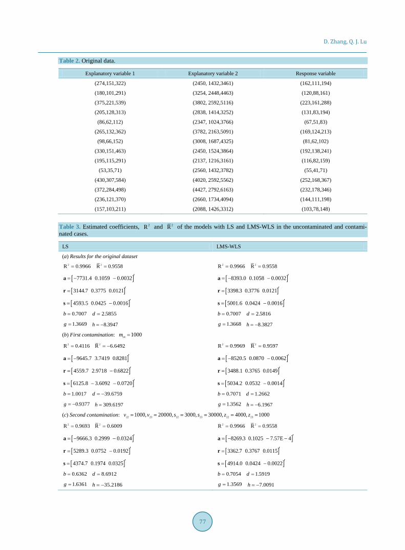
6.2. Example 2 This example consists of 14 fuzzy observations with two fuzzy explanatory variables and one fuzzy response variable from Wu [27], which is listed in Table 2. In this example, we set three different fuzzy numbers in the dataset, respectively, higher fuzzy extent, median fuzzy extent and lower fuzzy extent [28]. The setting is as follows:

2 1, ,531 6, ,1021 11, ,143

i i

i

i

i

λ ρ

== = =

=

LS and LMS-WLS estimates are reported in Table 3, in the first and second column respectively, obtained in correspondence to different types of outliers in the datasets.

LMS-WLS estimates do not noticeably change regardless of the absence or presence of outliers that is the same as the previou-s example, thus proving the effectiveness of the estimation procedure proposed.

If there is an outlier in the centers of output variable (Table 3, the case (b)), LS estimate of the coefficient vectors , ,a r s are strongly biased, and the estimates respectively for , , ,b d g h are also marginally affected. As a consequence, the goodness of fit is rather low. When we contaminate data with outliers in centers of both input variables and output variable (Table 3, the case (e)), the results are similar.

If we contaminate the vector X (Table 3, the case (c)) with a single outlier, LS produces biased estimates re-spectively for , ,a r s , while the estimates for the model of the spreads are unaffected.

If there is an outlier in the left spreads of output variable (Table 3, the case (d)), the estimates for ,b d are affected. Similar conclusions a-are drawn when we contaminate the vector of the right spreads of output variable (Table 3, the case (f)).

When we consider the more general cases (Table 3, the case (g) and Table 3, the case (h)), LS estimates are strongly biased with respect to the estimates obtained with the original dataset. As a consequence, also the fit performance of model is quite poor.

D. Zhang, Q. J. Lu

76

Table 1. Estimated coefficients, 2R and 2R of the models with LS and LMS-WLS in the uncontaminated and contami-nated cases.

LS LMS-WLS

(a) Results for the original dataset

2R 0.9998= 2R 0.9993=

2R 0.9998= 2R 0.9993=

[ ]3.0656 2.8189 ′=a [ ]17.1733 2.8189 ′=a

[ ]0.4726 2.0454 ′= −r [ ]14.5798 2.0453 ′= −r 0.0199b = 5.0701d = 0.0199b = 5.0718d =

(b) First contamination: 1 200m =

2R 0.5200= 2R 0.6800= −

2R 0.9998= 2R 0.9993=

[ ]19.3655 10.8131 ′= −a [ ]38.2321 2.8536 ′=a

[ ]68.7214 0.1805 ′= −r [ ]35.446 2.09 359 ′= −r 0.0145b = − 8.1600d = 0.0090b = 6.1345d =

(c) Second contamination: 4 35l =

2R 0.9824= 2R 0.9384=

2R 0.9999= 2R 0.9997=

[ ]21.1714 2.8391 ′=a [ ]3.7456 2.8638 ′=a

[ ]18.8493 2.0453 ′= −r [ ]1.7746 2.0544 ′= −r 0.1198b = − 19.9057d = 0.0254b = 4.4811d =

(d) Third contamination: 72 50v =

2R 0.9448= 2R 0.8068=

2R 0.9998= 2R 0.9993=

[ ]20.9816 0.2429 ′= −a [ ]5.7215 2.7728 ′=a

[ ]3.5042 1.9158 ′=r [ ]2.8617 2.0473 ′= −r 0.0237b = 4.7585d = 0.0197b = 5.0722d =

(e) Fourth contamination: 42 60s =

2R 0.3050= 2R 1.4325= −

2R 0.9999= 2R 0.9997=

[ ]3.5987 2.3819 ′= −a [ ]17.2289 2.8638 ′= −a

[ ]33.025 11.0818 ′=r [ ]19.1990 2.0544 ′=r 0.0362b = 3.7441d = 0.0254b = 4.4812d =

(f) Fifth contamination: 42 2 550, 60, 30s m l= = = 2R 0.5253=

2R 0.6615= − 2R 0.9999=

2R 0.9997=

[ ]5.1354 3.5968 ′= −a [ ]16.2176 2.8638 ′= −a

[ ]10.5551 1.6116 ′=r [ ]18.1777 2.0547 ′=r 0.0477b = − 13.4245d = 0.0272b = 4.2101d =

7. Conclusions The main problem that is investigated in this paper is to give a suitable method to deal with fuzzy data contami-nated by outliers, the fuzzy extent of which may be different. In this regard, a fuzzy regression model with fuzzy output and fuzzy inputs has been proposed. Then on the basis of the Least Median Squares-Weighted Least

D. Zhang, Q. J. Lu

77

Table 2. Original data.

Explanatory variable 1 Explanatory variable 2 Response variable

(274,151,322) (2450, 1432,3461) (162,111,194)

(180,101,291) (3254, 2448,4463) (120,88,161)

(375,221,539) (3802, 2592,5116) (223,161,288)

(205,128,313) (2838, 1414,3252) (131,83,194)

(86,62,112) (2347, 1024,3766) (67,51,83)

(265,132,362) (3782, 2163,5091) (169,124,213)

(98,66,152) (3008, 1687,4325) (81,62,102)

(330,151,463) (2450, 1524,3864) (192,138,241)

(195,115,291) (2137, 1216,3161) (116,82,159)

(53,35,71) (2560, 1432,3782) (55,41,71)

(430,307,584) (4020, 2592,5562) (252,168,367)

(372,284,498) (4427, 2792,6163) (232,178,346)

(236,121,370) (2660, 1734,4094) (144,111,198)

(157,103,211) (2088, 1426,3312) (103,78,148)

Table 3. Estimated coefficients, 2R and 2R of the models with LS and LMS-WLS in the uncontaminated and contami-nated cases.

LS LMS-WLS

(a) Results for the original dataset 2R 0.9966=

2R 0.9558= 2R 0.9966=

2R 0.9558=

[ ]7731.4 0.1059 0.0032 ′= − −a [ ]8393.0 0.1058 0.0032 ′= − −a

[ ]3144.7 0.3775 0.0121 ′=r [ ]3398.3 0.3776 0.0121 ′=r

[ ]4593.5 0.0425 0.0016 ′= −s [ ]5001.6 0.0424 0.0016 ′= −s 0.7007b = 2.5855d = 0.7007b = 2.5816d = 1.3669g = 8.3947h = − 1.3668g = 8.3827h = −

(b) First contamination: 14 1000m = 2R 0.4116=

2R 6.6492= − 2R 0.9969=

2R 0.9597=

[ ]9645.7 3.7419 0.8281 ′= −a [ ]8520.5 0.0870 0.0062 ′= − −a

[ ]4559.7 2.9718 0.6822 ′= −r [ ]3488.1 0.3765 0.0149 ′=r

[ ]6125.8 3.6092 0.0720 ′= − −s [ ]5034.2 0.0532 0.0014 ′= −s 1.0017b = 39.6759d = − 0.7071b = 1.2662d =

0.9377g = − 309.6197h = 1.3562g = 6.1967h = − (c) Second contamination: 22 23 22 23 22 231000, 20000, 3000, 30000, 4000, 1000v v s s z z= = = = = =

2R 0.9693= 2R 0.6009=

2R 0.9966= 2R 0.9558=

[ ]9666.3 0.2999 0.0324 ′= − −a [ ]8269.3 0.1025 7.57E 4 ′= − − −a

[ ]5289.3 0.0752 0.0192 ′= −r [ ]3362.7 0.3767 0.0115 ′=r

[ ]4374.7 0.1974 0.0325 ′=s [ ]4914.0 0.0424 0.0022 ′= −s 0.6362b = 8.6912d = 0.7054b = 1.5919d = 1.6361g = 35.2186h = − 1.3569g = 7.0091h = −

D. Zhang, Q. J. Lu

78

Continued

(d) Third contamination: 10 300l = 2R 0.9451=

2R 0.2863= 2R 0.9960=

2R 0.9480=

[ ]7729.5 0.1154 0.0075 ′= − −a [ ]8424.5 0.1076 0.0037 ′= − −a

[ ]3161.8 0.3136 0.0120 ′=r [ ]3428.9 0.3700 0.0121 ′=r

[ ]4575.2 0.1019 0.0016 ′= −s [ ]5002.0 0.0502 0.0016 ′= −s 0.2385b = 81.9706d = 0.7008b = 2.4828d = 1.3209g = 2.0719h = 1.3740g = 9.3926h = −

(e) Forth contamination: 33 240000, 500s m= = 2R 0.7683=

2R 2.0121= − 2R 0.9970=

2R 0.9610=

[ ]1035.6 0.6655 0.3505 ′= − −a [ ]10712 0.0900 0.0061 ′= −a

[ ]5392.6 0.2326 0.0035 ′= −r [ ]5809.6 0.3539 0.0098 ′=r

[ ]5013.7 0.1608 0.1225 ′= −s [ ]4910.1 0.0557 0.0033 ′= −s 0.1976b = 32.7932d = 0.6791b = 3.6677d = 0.3423g = 167.4266h = 1.4368g = 12.8086h = −

(f) Fifth contamination: 7 600u = 2R 0.7713=

2R 1.9731= − 2R 0.9963=

2R 0.9519=

[ ]7700.6 0.0730 0.0175 ′= − −a [ ]8339.3 0.1058 0.0033 ′= − −a

[ ]3164.1 0.1921 0.0190 ′=r [ ]3494.0 0.3762 0.0121 ′=r

[ ]4510.7 0.1285 0.0123 ′=s [ ]4952.0 0.0429 0.0015 ′= −s 0.6462b = 11.9113d = 0.7041b = 1.9301d = 1.0514g = 64.1119h = 1.3683g = 8.6311h = −

(g) Sixth contamination: 5 14700, 400m l= = 2R 0.4042=

2R 6.7454= − 2R 0.9967=

2R 0.9571=

[ ]7154.2 0.9097 0.3753 ′= − −a [ ]8425.1 0.0978 0.0097 ′= − −a

[ ]3687.5 1.1725 0.0469 ′= − −r [ ]3443.9 0.3619 0.0139 ′=r

[ ]3347.1 0.7142 0.2380 ′=s [ ]4981.3 0.0597 0.0012 ′=s 0.4785b = − 79.4693d = 0.7207b = 1.6215d = −

0.2591g = 244.8664h = 1.3361g = 0.8608h = − (h) Seventh contamination: 22 7 51000, 500, 400v m u= = =

2R 0.2595= 2R 8.6265= −

2R 0.9960= 2R 0.9480=

[ ]7637.4 0.1047 0.0260 ′= − − −a [ ]8333.2 0.1238 0.0119 ′= − −a

[ ]3358.6 0.6236 0.0179 ′= −r [ ]3398.9 0.3463 0.0115 ′=r

[ ]4205.7 0.4381 0.0619 ′=s [ ]4937.7 0.0560 0.0034 ′=s 0.4172b = 23.9003d = 0.7227b = 2.5196d = − 0.6874g = 117.2824h = 1.3668g = 5.5669h = −

Squares estimation procedure, we introduce a robust version of the proposed model. In order to analyze the per-formance of our model, we also suggest a suitable goodness of fit index, and its adjusted version, which is effec-tive for the model selection. The proposed model was applied in two examples, the results of which show that

D. Zhang, Q. J. Lu

79

our model outperforms the fuzzy regression model estimated with LS method in the presence of different typol-ogies outliers. In addition, the proposed model is applicable for all kinds of fuzzy numbers.

In the future, we will consider other robust regression approaches that usually are used in standard (non-fuzzy) regression analysis, for fuzzy linear regression analysis, such as the least trimmed squares. In addition, we will extend our robust fuzzy linear regression model with fuzzy inputs and output to robust non-linear regression models with fuzzy inputs and fuzzy output.

References [1] Tanaka, H., Uejima, S. and Asai, K. (1982) Linear Regression Analysis with Fuzzy Model. IEEE Transactions on Sys-

tems Man and Cybernetics, 12, 903-907. http://dx.doi.org/10.1109/TSMC.1982.4308925 [2] Diamond, P. (1988) Fuzzy Least Squares. Information Sciences, 46, 141-157.

http://dx.doi.org/10.1016/0020-0255(88)90047-3 [3] Shakouri, H. and Nadimia, R. (2009) A Novel Fuzzy Linear Regression Model Based on A Non-Equality Possibility

Index and Optimum Uncertainty. Applied Soft Computing, 9, 590-598. http://dx.doi.org/10.1016/j.asoc.2008.08.005 [4] Celmins, A. (1987) Multidimensional Least-Squares Fitting of Fuzzy Models. Mathematical Modelling, 9, 669-690.

http://dx.doi.org/10.1016/0270-0255(87)90468-4 [5] Chang, P.T. and Lee, E.S. (1996) A Generalized Fuzzy Weighted Least-Squares Regression. Fuzzy Sets and Systems,

82, 289-298. http://dx.doi.org/10.1016/0165-0114(95)00284-7 [6] Chang, Y.H. (2001) Hybrid Fuzzy Least-Squares Regression Analysis and Its Reliability Measures. Fuzzy Sets and

Systems, 119, 225-246. http://dx.doi.org/10.1016/S0165-0114(99)00092-5 [7] Coppi, R. and D’Urso, P. (2003) Regression Analysis with Fuzzy Informational Paradigm: A Least-Squares Approach

Using Membership Function Information. International Journal of Pure and Applied Mathematics, 8, 279-306. [8] Coppi, R., D’Urso, P., Giordani, P. and Santoro, A. (2006) Least Squares Estimation of a Linear Regression Model

with LR Fuzzy Response. Computational Statistics and Data Analysis, 51, 267-286. http://dx.doi.org/10.1016/j.csda.2006.04.036

[9] D’Urso, P. (2003) Linear Regression Analysis for Fuzzy/Crisp Input and Fuzzy/Crisp Output Data. Computational Statistics and Data Analysis, 42, 47-72. http://dx.doi.org/10.1016/S0167-9473(02)00117-2

[10] D’Urso, P. and Gastaldi, T. (2000) A Least-Squares Approach to Fuzzy Linear Regression Analysis. Computational Statistics and Data Analysis, 34, 427-440. http://dx.doi.org/10.1016/S0167-9473(99)00109-7

[11] Watada, J. and Yabuuchi, Y. (1995) Fuzzy Robust Regression Analysis Based on a Hyperelliptic Function. Journal of the Operations Research Society of Japan, 39, 512-524. http://dx.doi.org/10.1109/fuzzy.1995.409931

[12] Yang, M.S. and Ko, C.H. (1997) On Cluster-Wise Fuzzy Regression Analysis. IEEE Transactions on Systems Man and Cybernetics Part B, 27, 1-13. http://dx.doi.org/10.1109/3477.552181

[13] Oussalah, M. and De Schutter, J. (2002) Robust Fuzzy Linear Regression and Application for Contact Identification. Intelligent Automation and Soft Computing, 8, 31-39. http://dx.doi.org/10.1080/10798587.2002.10644195

[14] Yang, M.S. and Liu, H.H. (2003) Fuzzy Least Squares Algorithms for Interactive Fuzzy Linear Regression Models. Fuzzy Sets and Systems, 135, 305-316. http://dx.doi.org/10.1016/S0165-0114(02)00123-9

[15] Şanli, K. and Apaydin, A. (2004) The Fuzzy Robust Regression Analysis, the Case of Fuzzy Data Sethas Outlier. Gazi University Journal of Science, 17, 71-84.

[16] Varga, Š. (2007) Robust Estimations in Classical Regression Models versus Robust Estimations in Fuzzy Regression Models. Kybernetika, 43, 503-508.

[17] Choi, S.H. and Buckley, J.J. (2008) Fuzzy Regression Using Least Absolute Deviation Estimators. Soft Computing— A Fusion of Foundations, Methodologies and Applications, 12, 257-263.

[18] Kula, K.Ş. and Apaydin, A. (2008) Fuzzy Robust Regression Analysis Based on the Ranking of Fuzzy Sets. Inter- na-tional Journal Uncertainty, Fuzziness and Knowledge-Based Systems, 16, 663-681. http://dx.doi.org/10.1142/S0218488508005558

[19] Modarres, M., Nasrabadi, E. and Nasrabadi, M.M. (2004) Fuzzy Linear Regression Analysis from the Point of View Risk. International Journal Uncertainty, Fuzziness and Knowledge-Based Systems, 12, 635-649. http://dx.doi.org/10.1142/S0218488504003120

[20] Modarres, M., Nasrabadi, E. and Nasrabadi, M.M. (2005) Fuzzy Linear Regression with Least Squares Errors. Applied Mathematics and Computation, 163, 977-989. http://dx.doi.org/10.1016/j.amc.2004.05.004

[21] Nasrabadi, E. and Hashemi, S.M. (2008) Robust Fuzzy Regression Analysis Using Neural Networks. International

D. Zhang, Q. J. Lu

80

Journal Uncertainty, Fuzziness and Knowledge-Based Systems, 16, 579-598. http://dx.doi.org/10.1142/S021848850800542X

[22] Hu, Y.C. (2009) Functional-Link Nets with Genetic-Algorithm-Based Learning for Robust Nonlinear Interval Regres-sion Analysis. Neurocomputing, 72, 1808-1816. http://dx.doi.org/10.1016/j.neucom.2008.07.002

[23] Maronna, R.A. and Yohai, V.J. (2013) Robust Functional Linear Regression Based on Splines. Computational Statis-tics and Data Analysis, 65, 46-55. http://dx.doi.org/10.1016/j.csda.2011.11.014

[24] D’Urso, P., Massari, R. and Santoro, A. (2011) Robust Fuzzy Regression Analysis. Information Sciences, 181, 4154- 4174. http://dx.doi.org/10.1016/j.ins.2011.04.031

[25] Chachi, J. and Roozbeh, M. (2015) A Fuzzy Robust Regression Approach Applied to Bedload Transport Data. Com-munications in Statistics-Simulation and Computation, Online Publication Date: 7 April 2015. http://dx.doi.org/10.1080/03610918.2015.1010002

[26] Wang, L. (2013) Robust Estimation Methods and Applicative Examples of Linear Regression Models. Master Thesis, Shandong University, Jinan.

[27] Wu, H.C. (2003) Linear Regression Analysis for Fuzzy Input and Output Data Using the Extension Principle. Comput-ers and Mathematics with Applications, 45, 1849-1859. http://dx.doi.org/10.1016/S0898-1221(03)90006-X

[28] Ren, L.L. and Lu, Q.J. (2013) E-Commerce Trading Volume Forecast Based on Fuzzy Linear Regression. Statistics and Decision, 3, 31-34.