risk sharing in traditional construction contracts for building projects

“RISK SHARING IN TRADITIONAL CONSTRUCTION CONTRACTS FOR BUILDING PROJECTS.” A CONTRACTOR’S PERSPECTIVE IN THE GREEK CONSTRUCTION INDUSTRY.

ENSCHEDE, 29-04-2015 Dimitrios Kordas (M-CME/s1231901)

MSc: Construction Management and Engineering

1. INTRODUCTION

29-04-2015 2

29-04-2015 3

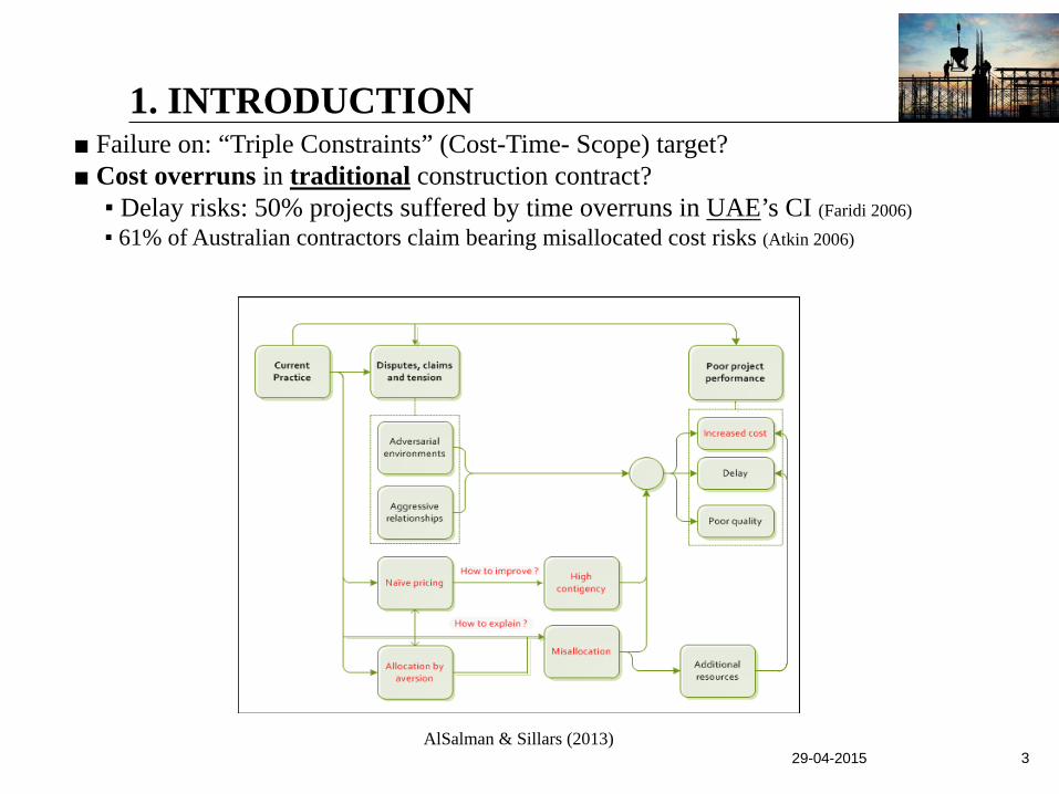
■ Failure on: “Triple Constraints” (Cost-Time- Scope) target? ■ Cost overruns in traditional construction contract?

▪ Delay risks: 50% projects suffered by time overruns in UAE’s CI (Faridi 2006) ▪ 61% of Australian contractors claim bearing misallocated cost risks (Atkin 2006)

AlSalman & Sillars (2013)

1. INTRODUCTION

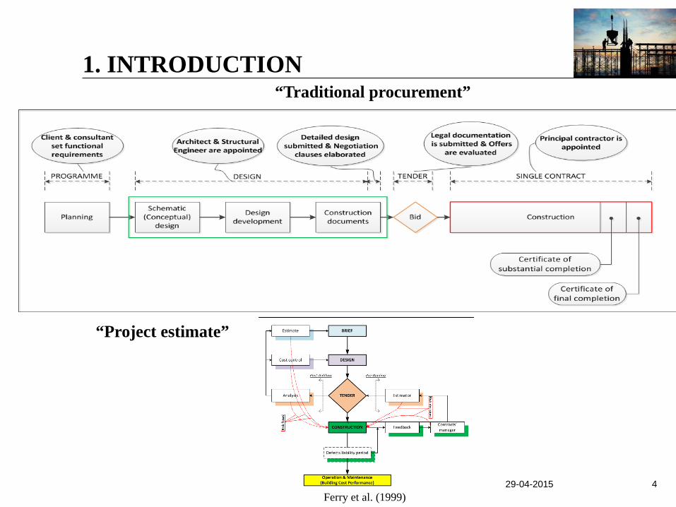
“Traditional procurement”

29-04-2015 4

Ferry et al. (1999)

1. INTRODUCTION

“Project estimate”

29-04-2015 5

“A practical case in traditional building procurement in the Greek CI” Step 1: Client submits a Request for Proposals invitation Step 2: Contractors: “Closed books” bid-competition Step 3: Client and awarded contractor: “Open books” Post-bid 3.1 Compensation mechanism agreement 3.2 Risk sharing agreement

For the contractor: Price (Contract value) = Fixed amount (Base estimate) + Profit

For the client: Price = Contract value ± 30-35%×Contract value

“Maximum cost risk allowance”

1. INTRODUCTION

Pipattanapiwong (2004)

■ No risks → Fixed amount paid. ■ On-site risks → always →

sharing agreement → if unfair risk allocation by client → contractors: reserve amounts (contingencies) or arbitration path.

High contingencies pre-bid ↔ More/Less risks shared

Revise profits & estimates? ⇒ Project cost performance Cotnigencies

Contingencies ↔ Incentive profits Contingency reduction →

Project delivery efficiency

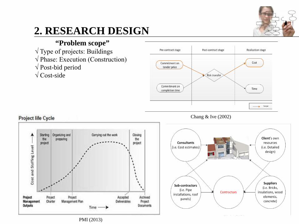
2. RESEARCH DESIGN

29-04-2015 6

“Problem scope” √ Type of projects: Buildings √ Phase: Execution (Construction) √ Post-bid period √ Cost-side

Chang & Ive (2002)

PMI (2013)

29-04-2015 7

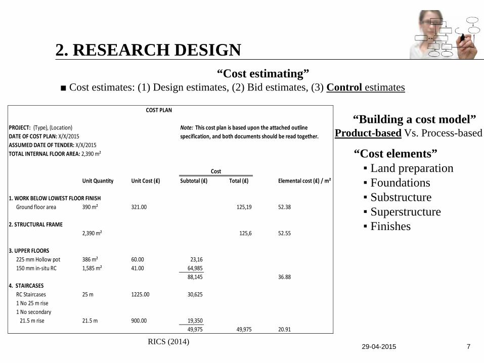
“Cost estimating” ■ Cost estimates: (1) Design estimates, (2) Bid estimates, (3) Control estimates

2. RESEARCH DESIGN

“Building a cost model” Product-based Vs. Process-based

COST PLAN

PROJECT: (Type), (Location) Note: This cost plan is based upon the attached outlineDATE OF COST PLAN: X/X/2015 specification, and both documents should be read together.ASSUMED DATE OF TENDER: X/X/2015TOTAL INTERNAL FLOOR AREA: 2,390 m²

CostUnit Quantity Unit Cost (₤) Subtotal (₤) Total (₤) Elemental cost (₤) / m²

1. WORK BELOW LOWEST FLOOR FINISH Ground floor area 390 m² 321.00 125,19 52.38

2. STRUCTURAL FRAME2,390 m² 125,6 52.55

3. UPPER FLOORS 225 mm Hollow pot 386 m² 60.00 23,16150 mm in-situ RC 1,585 m² 41.00 64,985

88,145 36.884. STAIRCASES

RC Staircases 25 m 1225.00 30,6251 No 25 m rise1 No secondary

21.5 m rise 21.5 m 900.00 19,35049,975 49,975 20.91

“Cost elements” ▪ Land preparation ▪ Foundations ▪ Substructure ▪ Superstructure ▪ Finishes

RICS (2014)

29-04-2015 8

Ferry et al. (1999)

2. RESEARCH DESIGN “Components in a project cost estimate”

1. Identification 2. Assessment = Analysis + Evaluation 3. Monitoring 4. Control

29-04-2015 9

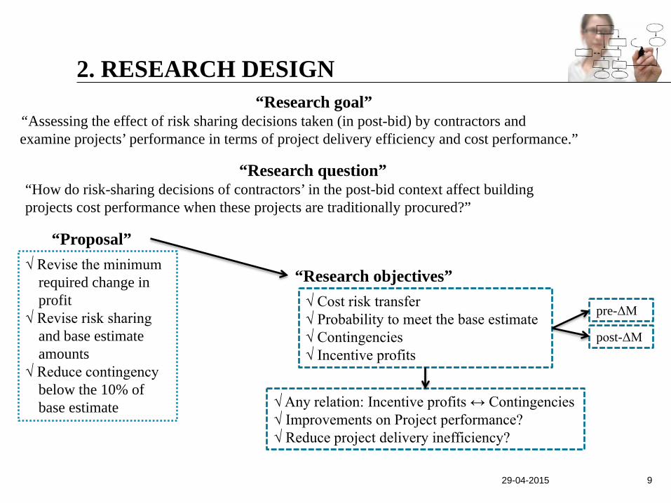
2. RESEARCH DESIGN “Research goal”

“Assessing the effect of risk sharing decisions taken (in post-bid) by contractors and examine projects’ performance in terms of project delivery efficiency and cost performance.”

“Research question” “How do risk-sharing decisions of contractors’ in the post-bid context affect building projects cost performance when these projects are traditionally procured?”

√ Revise the minimum required change in profit

√ Revise risk sharing and base estimate amounts

√ Reduce contingency below the 10% of base estimate

“Research objectives” √ Cost risk transfer √ Probability to meet the base estimate √ Contingencies √ Incentive profits

√ Any relation: Incentive profits ↔ Contingencies √ Improvements on Project performance? √ Reduce project delivery inefficiency?

pre-ΔΜ

pοst-ΔΜ

“Proposal”

29-04-2015 10

Joustra (2010)

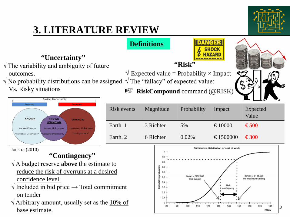
3. LITERATURE REVIEW Definitions

“Uncertainty” √ The variability and ambiguity of future

outcomes. √ No probability distributions can be assigned

Vs. Risky situations

“Risk” √ Expected value = Probability × Impact √ The “fallacy” of expected value:

Risk events Magnitude Probability Impact Expected Value

Earth. 1 3 Richter 5% € 10000 € 500

Earth. 2 6 Richter 0.02% € 1500000 € 300

RiskCompound command (@RISK)

“Contingency” √ A budget reserve above the estimate to

reduce the risk of overruns at a desired confidence level.

√ Included in bid price → Total commitment on tender

√ Arbitrary amount, usually set as the 10% of base estimate.

29-04-2015 11

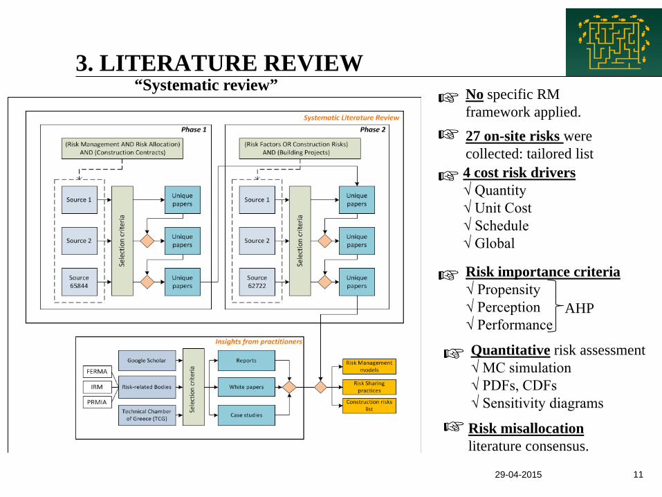
3. LITERATURE REVIEW “Systematic review” No specific RM

framework applied. 27 on-site risks were collected: tailored list 4 cost risk drivers √ Quantity √ Unit Cost √ Schedule √ Global

Risk importance criteria √ Propensity √ Perception √ Performance

Quantitative risk assessment √ MC simulation √ PDFs, CDFs √ Sensitivity diagrams

AHP

Risk misallocation literature consensus.

12

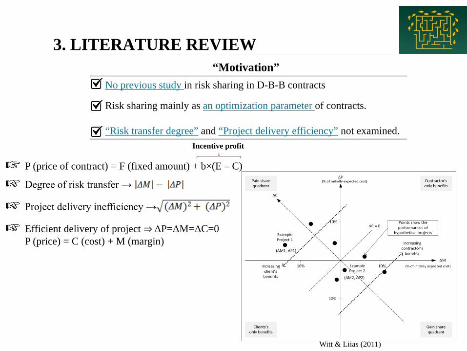
No previous study in risk sharing in D-B-B contracts

Risk sharing mainly as an optimization parameter of contracts.

“Risk transfer degree” and “Project delivery efficiency” not examined.

P (price of contract) = F (fixed amount) + b×(E – C)

Incentive profit

3. LITERATURE REVIEW “Motivation”

Degree of risk transfer →

Project delivery inefficiency →

Witt & Liias (2011)

Efficient delivery of project ⇒ ΔP=ΔM=ΔC=0 P (price) = C (cost) + M (margin)

29-04-2015 13

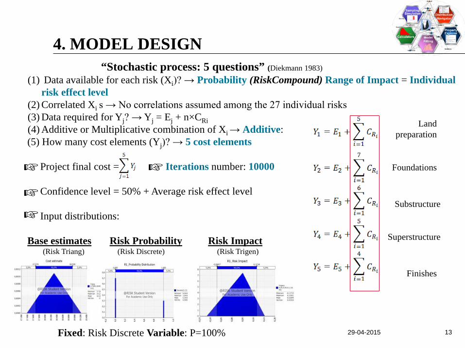
4. MODEL DESIGN “Stochastic process: 5 questions” (Diekmann 1983)

(1) Data available for each risk (Xi)? → Probability (RiskCompound) Range of Impact = Individual risk effect level

(2) Correlated Xi s → No correlations assumed among the 27 individual risks (3) Data required for Yj? → Yj = Ej + n×CRi (4) Additive or Multiplicative combination of Xi → Additive: (5) How many cost elements (Yj)? → 5 cost elements Project final cost = Iterations number: 10000 Confidence level = 50% + Average risk effect level Input distributions: Base estimates Risk Probability Risk Impact (Risk Triang) (Risk Discrete) (Risk Trigen)

Land preparation

Foundations

Substructure

Superstructure

Finishes

Fixed: Risk Discrete Variable: P=100%

29-04-2015

14

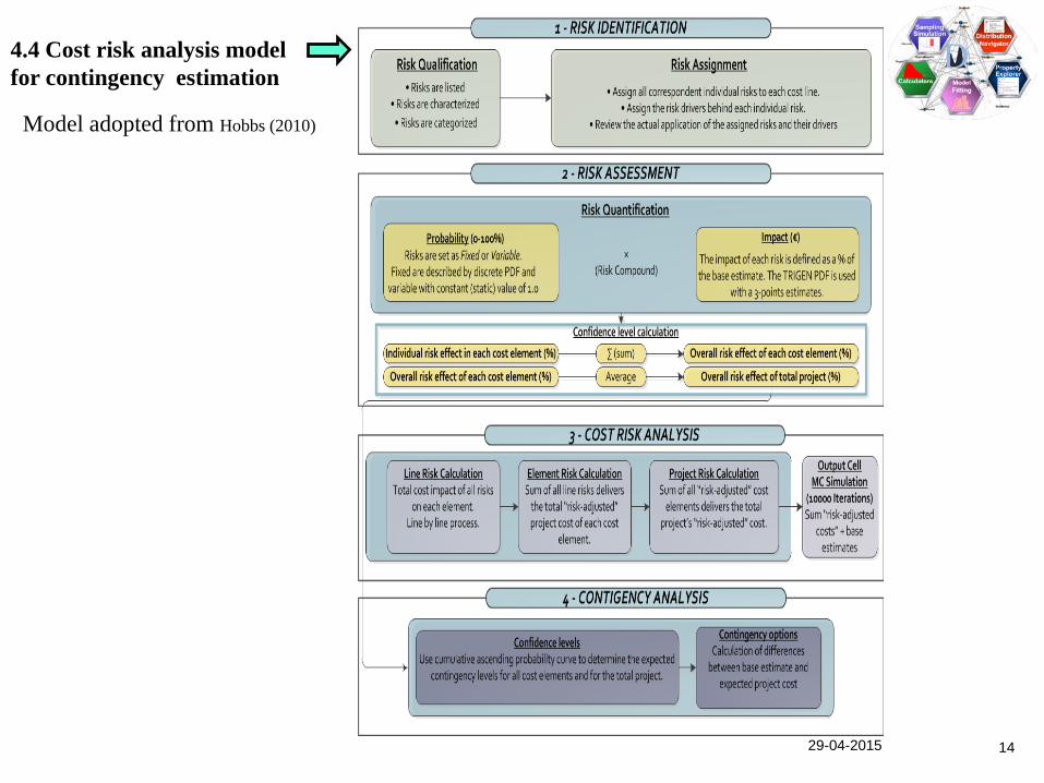
4.4 Cost risk analysis model for contingency estimation

Model adopted from Hobbs (2010)

29-04-2015 15

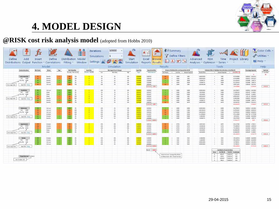
Construction phase Risk factors Drivers Type Risk Probability Input Distr. Risk impact (% on E change) Input Distr. Overall risk effect Amount of individual line cost impacted by risk (€) Estimated effect of individual risk on line item or Cost Risks (€) Percentage impacted Total CostOccuring Not occuring Discrete / 1 (F / V) Low Most likely High Trigen RiskCompound Risk Prob/ty × Cost line = Amount Impacted Overall effect × Amount impacted = Cost effect (€) E + Cost Risks

% (€) Land preparation R1 Quantity F 30% 70% 0 -5% 5% 10% 0,028488 0,008739 0,3 × 18300 5490 0,008738705 × 5490 47,97549008 0,002622 0,2621611

E (€) 18300 R2 Quantity F 30% 70% 0 -5% 5% 10% 0,028488 0,008739 0,3 × 18300 5490 0,008738705 × 5490 47,97549008 0,002622 0,2621611(-5%,+5%) 18300 R3 Quantity V 100% 0% 1 -5% 5% 10% 0,028488 0,028488 1 × 18300 18300 0,02848774 × 18300 521,3256419 0,028488 2,848774

R4 Quantity V 100% 0% 1 -5% 5% 10% 0,028488 0,028488 1 × 18300 18300 0,02848774 × 18300 521,3256419 0,028488 2,848774R5 Unit cost F 30% 70% 0 -10% 2% 10% 0,002814 0,001092 0,3 × 18300 5490 0,001092299 × 5490 5,996721855 0,000328 0,032769

0,075545 7,55% 1144,598986 6,2546393 19444,60

Foundations R6 Unit cost V 100% 0% 1 -10% 2% 10% 0,002814 0,002814 1 × 54900 54900 0,002813841 × 54900 154,4798472 0,002814 0,2813841E (€) 54900 R7 Global V 100% 0% 1 -5% 1% 5% 0,001407 0,001407 1 × 54900 54900 0,00140692 × 54900 77,23992359 0,001407 0,140692

(-2%,+2%) 54900 R8 Global V 100% 0% 1 -5% 1% 5% 0,001407 0,001407 1 × 54900 54900 0,00140692 × 54900 77,23992359 0,001407 0,140692R9 Global F 10% 90% 0 -5% 1% 5% 0,001407 0,000182 0,1 × 54900 5490 0,000182032 × 5490 0,999353697 1,82E-05 0,0018203R10 Quantity F 10% 90% 0 -5% 5% 10% 0,028488 0,002913 0,1 × 54900 5490 0,00291261 × 5490 15,99023084 0,000291 0,0291261R11 Quantity V 100% 0% 1 -5% 5% 10% 0,028488 0,028488 1 × 54900 54900 0,02848774 × 54900 1563,976926 0,028488 2,848774R12 Quantity F 30% 70% 0 -5% 5% 10% 0,028488 0,008739 0,3 × 54900 16470 0,008738705 × 16470 143,9264702 0,002622 0,2621611

0,045949 4,59% 2033,852675 3,7046497 56933,85

Substructure R13 Unit cost V 100% 0% 1 -10% 2% 10% 0,002814 0,002814 1 × 54900 54900 0,002813841 × 54900 154,4798472 0,002814 0,2813841E (€) 54900 R14 Unit cost F 40% 60% 0 -10% 2% 10% 0,002814 0,001456 0,4 × 54900 21960 0,001456253 × 21960 31,97931831 0,000583 0,0582501

(-7%,+7%) 54900 R15 Unit cost F 40% 60% 0 -10% 2% 10% 0,002814 0,001456 0,4 × 54900 21960 0,001456253 × 21960 31,97931831 0,000583 0,0582501R16 Schedule F 60% 40% 1 -10% 10% 50% 0,186049 0,112997 0,6 × 54900 32940 0,112996663 × 32940 3722,110068 0,067798 6,7797998R17 Schedule V 100% 0% 1 -10% 10% 50% 0,186049 0,186049 1 × 54900 54900 0,18604904 × 54900 10214,0923 0,186049 18,604904R18 Quantity V 100% 0% 1 -5% 5% 10% 0,028488 0,028488 1 × 54900 54900 0,02848774 × 54900 1563,976926 0,028488 2,848774

0,33326 33,32% 15718,61777 28,63 70618,62

Superstructure R19 Schedule F 50% 50% 0 -10% 10% 50% 0,186049 0,094126 0,5 × 45750 22875 0,09412622 × 22875 2153,137282 0,047063 4,706311E (€) 45750 R20 Schedule F 30% 70% 0 -10% 10% 50% 0,186049 0,056481 0,3 × 45750 13725 0,05648138 × 13725 775,2069424 0,016944 1,6944414

(-7%,+7%) 45750 R21 Schedule F 30% 70% 0 -10% 10% 50% 0,186049 0,056481 0,3 × 45750 13725 0,05648138 × 13725 775,2069424 0,016944 1,6944414R22 Global V 100% 0% 1 -5% 1% 5% 0,001407 0,001407 1 × 45750 45750 0,00140692 × 45750 64,36660299 0,001407 0,140692R23 Global V 100% 0% 1 -5% 1% 5% 0,001407 0,001407 1 × 45750 45750 0,00140692 × 45750 64,36660299 0,001407 0,140692

0,209903 20,99% 3832,284373 8,3765779 49582,28

Finishes R24 Schedule V 100% 0% 1 -10% 10% 50% 0,186049 0,186049 1 × 9150 9150 0,18604904 × 9150 1702,348716 0,186049 18,604904E (€) 9150 R25 Schedule V 100% 0% 1 -10% 10% 50% 0,186049 0,186049 1 × 9150 9150 0,18604904 × 9150 1702,348716 0,186049 18,604904

(-5%,+5%) 9150 R26 Unit cost V 100% 0% 1 -10% 2% 10% 0,002814 0,002814 1 × 9150 9150 0,002813841 × 9150 25,7466412 0,002814 0,2813841R27 Unit cost V 100% 0% 1 -10% 2% 10% 0,002814 0,002814 1 × 9150 9150 0,002813841 × 9150 25,7466412 0,002814 0,2813841

0,377726 37,72% 3456,190715 37,772576 12606,19

Overall 20,83% Contribution of cost risk drivers Driver Cost Risk (€) Total (€) Contribution

Q 4426,47 26185,54 0,17 Project final cost 209185,5 UC 430,41 26185,54 0,02

S 21044,45 26185,54 0,80G 284,21 26185,54 0,01

Overall risk level = Average (Risk effects)Confidence level= 50% + Overall risk level

Error range limits Input Distr. Triang

Error range limits Input Distr. Triang

Error range limits

Error range limits

Error range limits

Input Distr. Triang

Input Distr. Triang

Input Distr. Triang

Sum of output cells

@RISK cost risk analysis model (adopted from Hobbs 2010)

4. MODEL DESIGN

5. SURVEY DESIGN

29-04-2015 16

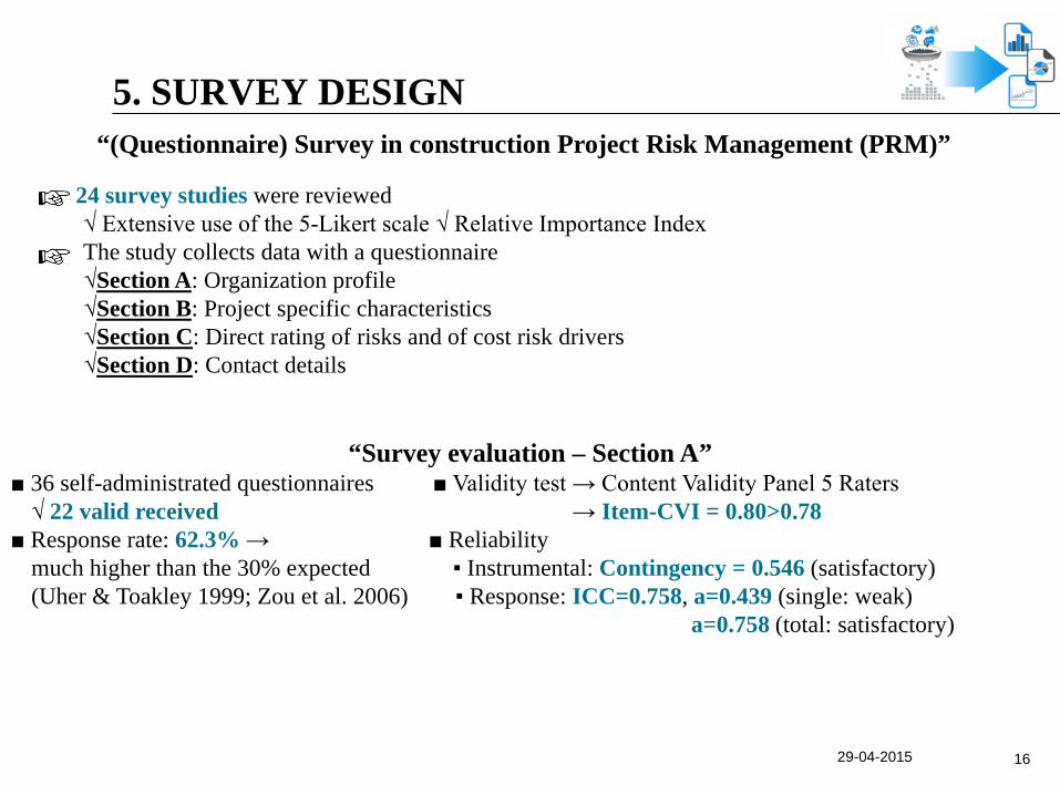
“(Questionnaire) Survey in construction Project Risk Management (PRM)” 24 survey studies were reviewed

√ Extensive use of the 5-Likert scale √ Relative Importance Index The study collects data with a questionnaire √Section A: Organization profile √Section B: Project specific characteristics √Section C: Direct rating of risks and of cost risk drivers √Section D: Contact details

“Survey evaluation – Section A” ■ 36 self-administrated questionnaires ■ Validity test → Content Validity Panel 5 Raters

√ 22 valid received → Item-CVI = 0.80>0.78 ■ Response rate: 62.3% → ■ Reliability

much higher than the 30% expected ▪ Instrumental: Contingency = 0.546 (satisfactory) (Uher & Toakley 1999; Zou et al. 2006) ▪ Response: ICC=0.758, a=0.439 (single: weak) a=0.758 (total: satisfactory)

29-04-2015 17

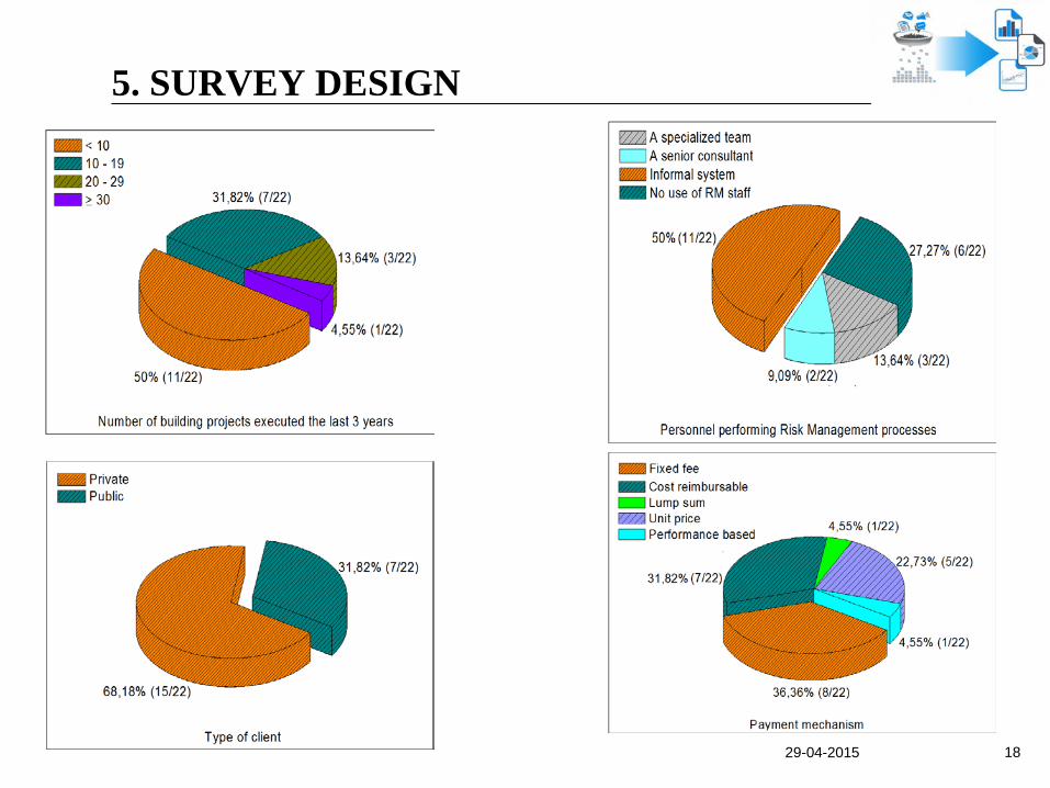
5. SURVEY DESIGN “Sample description”

29-04-2015

18

5. SURVEY DESIGN

29-04-2015

19

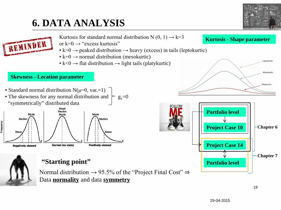
6. DATA ANALYSIS Kurtosis for standard normal distribution N (0, 1) → k=3 or k=0 → “excess kurtosis” ▪ k>0 → peaked distribution → heavy (excess) in tails (leptokurtic) ▪ k=0 → normal distribution (mesokurtic) ▪ k<0 → flat distribution → light tails (platykurtic)

▪ Standard normal distribution N(μ=0, var.=1) ▪ The skewness for any normal distribution and

“symmetrically” distributed data g1=0

Kurtosis - Shape parameter

Skewness - Location parameter

Normal distribution → 95.5% of the “Project Final Cost” ⇒ Data normality and data symmetry

“Starting point”

Portfolio level

Project Case 10

Project Case 14

Portfolio level Chapter 7

Chapter 6

20 29-04-2015

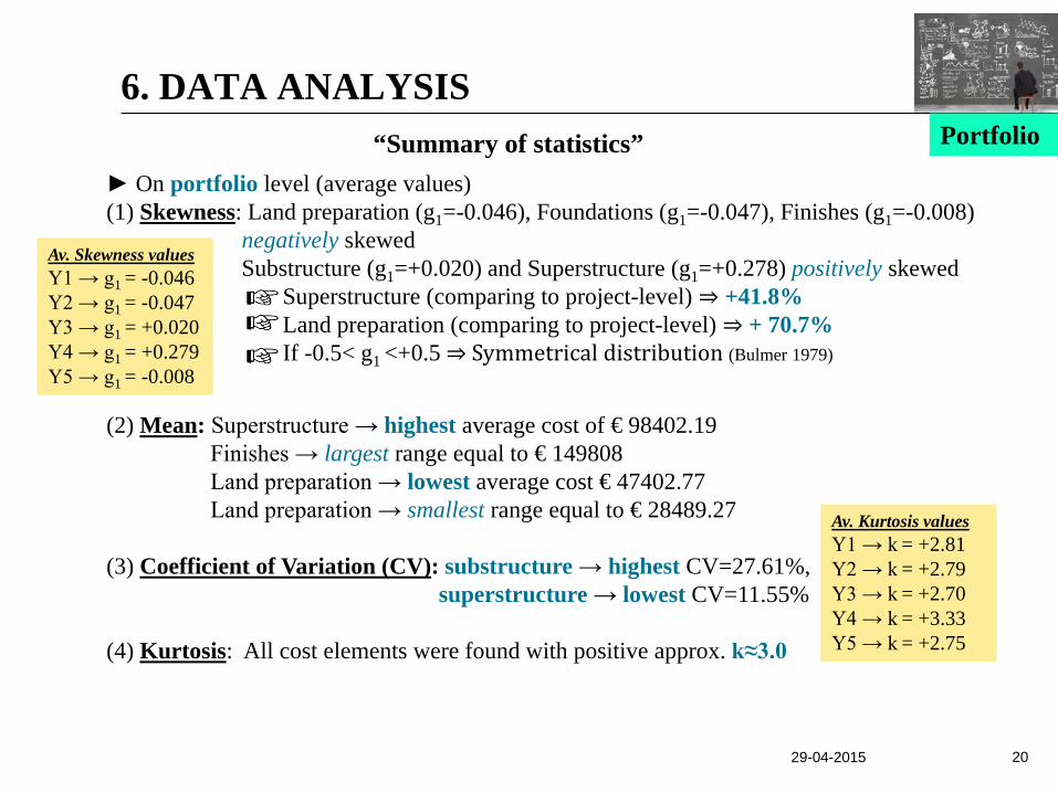
► On portfolio level (average values) (1) Skewness: Land preparation (g1=-0.046), Foundations (g1=-0.047), Finishes (g1=-0.008)

negatively skewed Substructure (g1=+0.020) and Superstructure (g1=+0.278) positively skewed Superstructure (comparing to project-level) ⇒ +41.8% Land preparation (comparing to project-level) ⇒ + 70.7% If -0.5< g1 <+0.5 ⇒ Symmetrical distribution (Bulmer 1979)

Av. Skewness values Y1 → g1 = -0.046 Y2 → g1 = -0.047 Y3 → g1 = +0.020 Y4 → g1 = +0.279 Y5 → g1 = -0.008

(2) Mean: Superstructure → highest average cost of € 98402.19 Finishes → largest range equal to € 149808 Land preparation → lowest average cost € 47402.77 Land preparation → smallest range equal to € 28489.27

(3) Coefficient of Variation (CV): substructure → highest CV=27.61%,

superstructure → lowest CV=11.55% (4) Kurtosis: All cost elements were found with positive approx. k≈3.0

Av. Kurtosis values Y1 → k = +2.81 Y2 → k = +2.79 Y3 → k = +2.70 Y4 → k = +3.33 Y5 → k = +2.75

6. DATA ANALYSIS “Summary of statistics” Portfolio

21

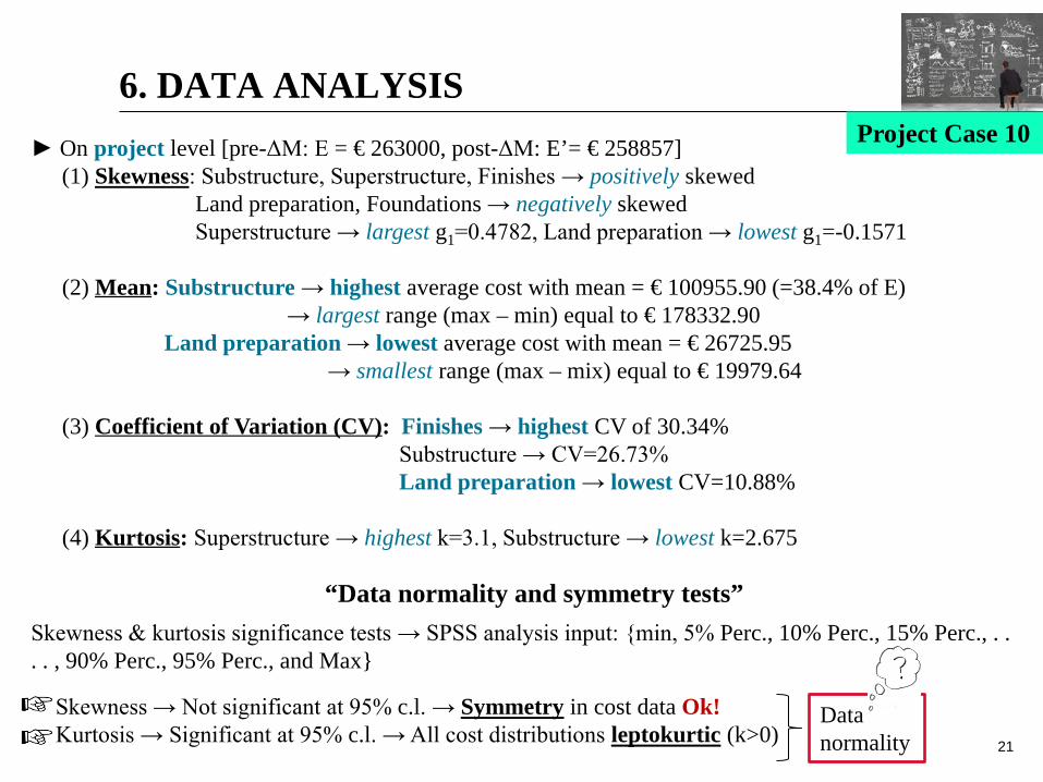
► On project level [pre-ΔΜ: Ε = € 263000, post-ΔΜ: E’= € 258857] (1) Skewness: Substructure, Superstructure, Finishes → positively skewed

Land preparation, Foundations → negatively skewed Superstructure → largest g1=0.4782, Land preparation → lowest g1=-0.1571

(2) Mean: Substructure → highest average cost with mean = € 100955.90 (=38.4% of E)

→ largest range (max – min) equal to € 178332.90 Land preparation → lowest average cost with mean = € 26725.95

→ smallest range (max – mix) equal to € 19979.64 (3) Coefficient of Variation (CV): Finishes → highest CV of 30.34%

Substructure → CV=26.73% Land preparation → lowest CV=10.88%

(4) Kurtosis: Superstructure → highest k=3.1, Substructure → lowest k=2.675

6. DATA ANALYSIS Project Case 10

“Data normality and symmetry tests” Skewness & kurtosis significance tests → SPSS analysis input: {min, 5% Perc., 10% Perc., 15% Perc., . . . . , 90% Perc., 95% Perc., and Max}

Skewness → Not significant at 95% c.l. → Symmetry in cost data Ok! Kurtosis → Significant at 95% c.l. → All cost distributions leptokurtic (k>0)

Data normality

29-04-2015 22

6. DATA ANALYSIS

“Normality tests”

All cost elements → Follow normal distribution pattern

Kolmogorov-Smirnov (K-S) and Shapiro-Wilk (S-W)

Project Case 10

29-04-2015 23

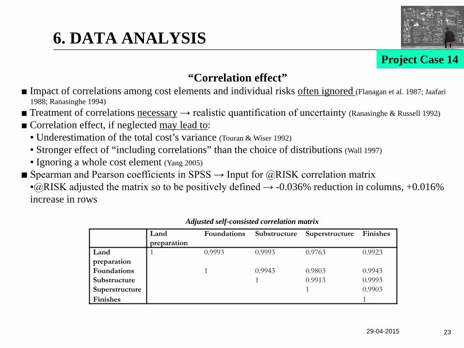
“Correlation effect” ■ Impact of correlations among cost elements and individual risks often ignored (Flanagan et al. 1987; Jaafari

1988; Ranasinghe 1994) ■ Treatment of correlations necessary → realistic quantification of uncertainty (Ranasinghe & Russell 1992) ■ Correlation effect, if neglected may lead to:

▪ Underestimation of the total cost’s variance (Touran & Wiser 1992) ▪ Stronger effect of “including correlations” than the choice of distributions (Wall 1997) ▪ Ignoring a whole cost element (Yang 2005)

■ Spearman and Pearson coefficients in SPSS → Input for @RISK correlation matrix ▪@RISK adjusted the matrix so to be positively defined → -0.036% reduction in columns, +0.016% increase in rows

Land preparation

Foundations Substructure Superstructure Finishes

Land preparation

1 0.9993 0.9993 0.9763 0.9923

Foundations 1 0.9943 0.9803 0.9943 Substructure 1 0.9913 0.9993 Superstructure 1 0.9903 Finishes 1

Adjusted self-consisted correlation matrix


24 29-04-2015

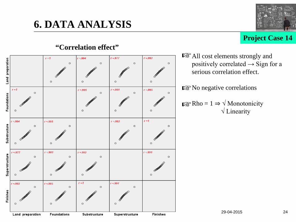
All cost elements strongly and positively correlated → Sign for a serious correlation effect. No negative correlations Rho = 1 ⇒ √ Monotonicity

√ Linearity

6. DATA ANALYSIS

“Correlation effect” Project Case 14

25

“Simulation results”

Probability meeting the estimate +7 % Increase Range of data captured in 90% +94.67% more cost data captured


■ @ the desired confidence level 71.57%

+3.39% higher estimate when including correlations

■ Two S-curves cross @ 50% c.l. ▪ Below 50% c.l. → tendency for underestimation (with) ▪ Above 50% c.l. → tendency for overestimation (with) Mean overestimated by +0.1% Variance increased by +3.4% SD increased by + 1.7% SE increased by +55.1 units → more outliers . . .

29-04-2015 26

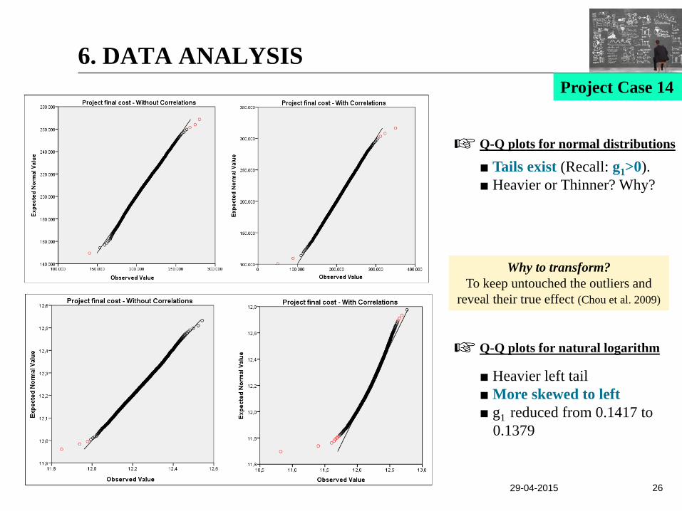
■ Tails exist (Recall: g1>0). ■ Heavier or Thinner? Why?

■ Heavier left tail ■ More skewed to left ■ g1 reduced from 0.1417 to

0.1379

Q-Q plots for normal distributions

Q-Q plots for natural logarithm

Why to transform? To keep untouched the outliers and

reveal their true effect (Chou et al. 2009)


29-04-2015 27

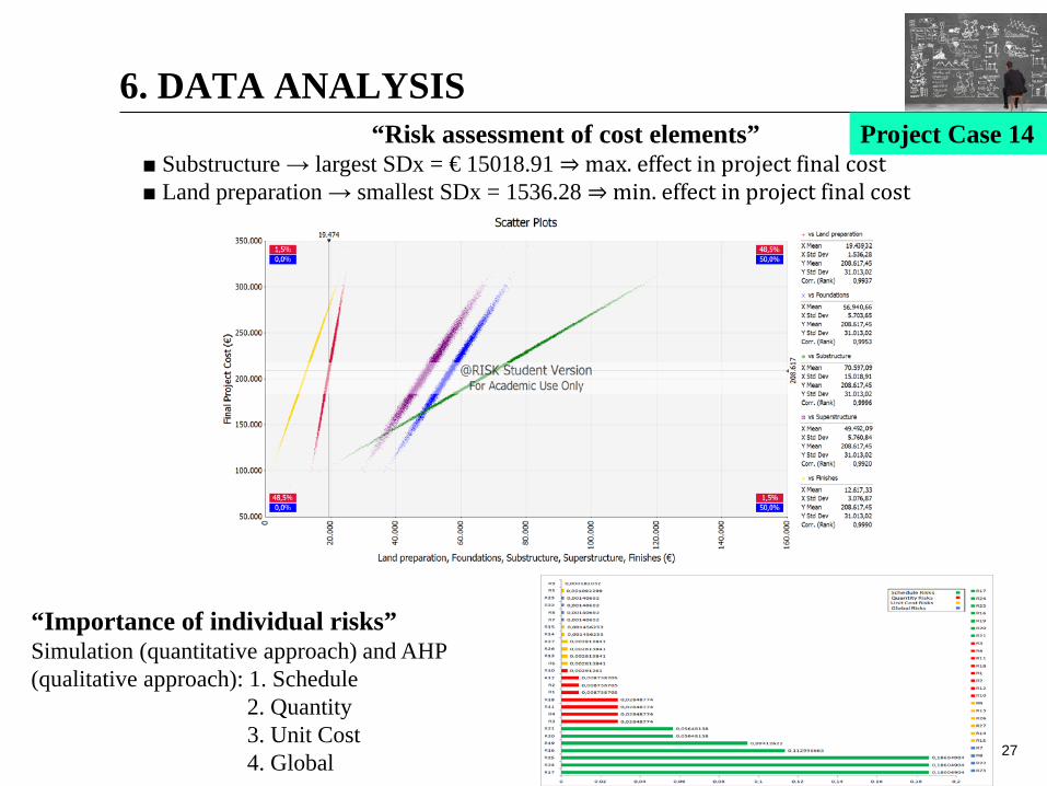
“Risk assessment of cost elements” ■ Substructure → largest SDx = € 15018.91 ⇒ max. effect in project final cost ■ Land preparation → smallest SDx = 1536.28 ⇒ min. effect in project final cost

6. DATA ANALYSIS

“Importance of individual risks” Simulation (quantitative approach) and AHP (qualitative approach): 1. Schedule

2. Quantity 3. Unit Cost 4. Global

Project Case 14

29-04-2015 28

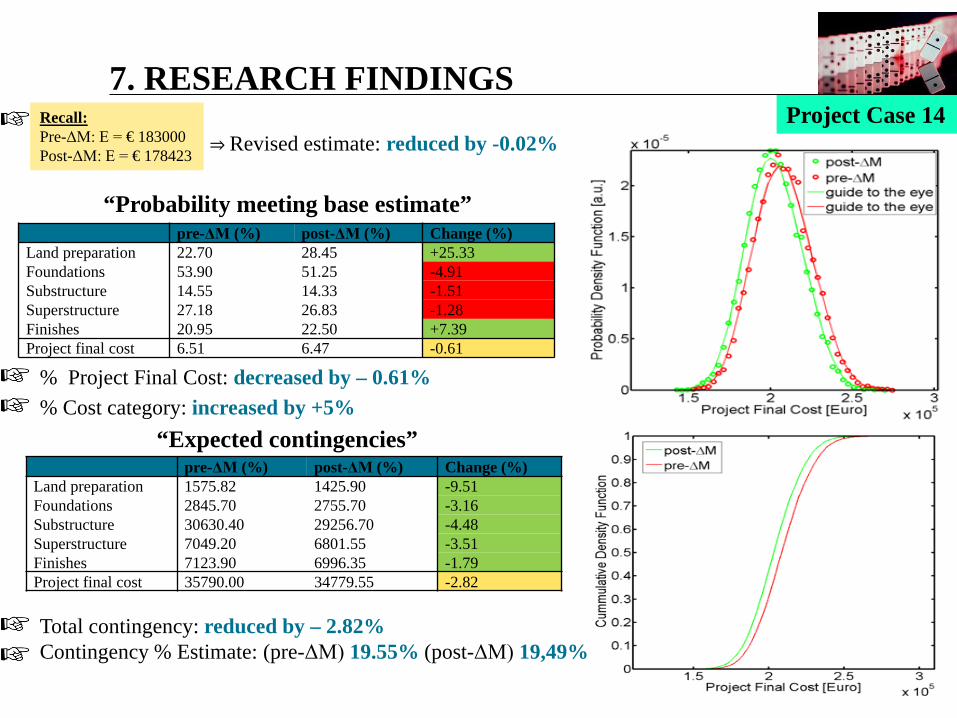
“Probability meeting base estimate”

pre-ΔΜ (%) post-ΔΜ (%) Change (%)

Land preparation 22.70 28.45 +25.33 Foundations 53.90 51.25 -4.91 Substructure 14.55 14.33 -1.51 Superstructure 27.18 26.83 -1.28 Finishes 20.95 22.50 +7.39 Project final cost 6.51 6.47 -0.61

pre-ΔΜ (%) post-ΔΜ (%) Change (%) Land preparation 1575.82 1425.90 -9.51 Foundations 2845.70 2755.70 -3.16 Substructure 30630.40 29256.70 -4.48 Superstructure 7049.20 6801.55 -3.51 Finishes 7123.90 6996.35 -1.79 Project final cost 35790.00 34779.55 -2.82

% Project Final Cost: decreased by – 0.61%

Total contingency: reduced by – 2.82% Contingency % Estimate: (pre-ΔΜ) 19.55% (post-ΔΜ) 19,49%

“Expected contingencies”

Recall: Pre-ΔΜ: Ε = € 183000 Post-ΔΜ: Ε = € 178423

⇒ Revised estimate: reduced by -0.02%

7. RESEARCH FINDINGS Project Case 14

% Cost category: increased by +5%

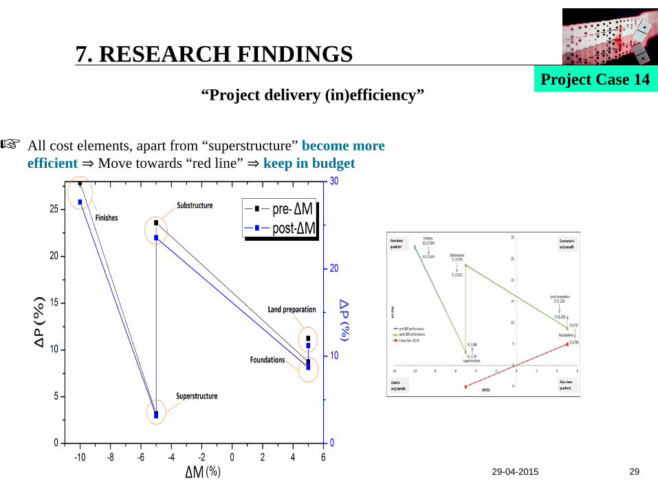
All cost elements, apart from “superstructure” become more efficient ⇒ Move towards “red line” ⇒ keep in budget

29-04-2015 29


“Project delivery (in)efficiency”

29-04-2015 30

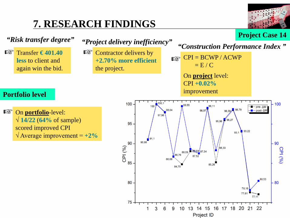
“Risk transfer degree” “Project delivery inefficiency” Transfer € 401.40 less to client and again win the bid.

Contractor delivers by +2.70% more efficient the project.


On project level: CPI +0.02% improvement

CPI = BCWP / ACWP = E / C

“Construction Performance Index ”

Portfolio level

On portfolio-level: √ 14/22 (64% of sample) scored improved CPI √ Average improvement = +2%

31

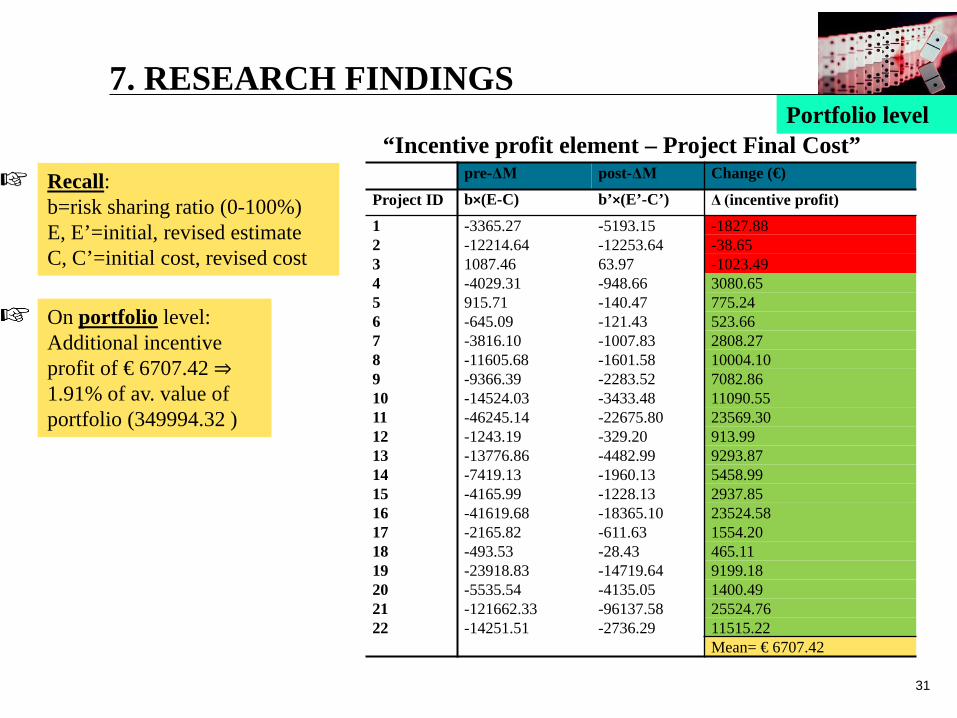
pre-ΔΜ post-ΔΜ Change (€)

Project ID b×(E-C) b’×(E’-C’) Δ (incentive profit) 1 -3365.27 -5193.15 -1827.88 2 -12214.64 -12253.64 -38.65 3 1087.46 63.97 -1023.49 4 -4029.31 -948.66 3080.65 5 915.71 -140.47 775.24 6 -645.09 -121.43 523.66 7 -3816.10 -1007.83 2808.27 8 -11605.68 -1601.58 10004.10 9 -9366.39 -2283.52 7082.86 10 -14524.03 -3433.48 11090.55 11 -46245.14 -22675.80 23569.30 12 -1243.19 -329.20 913.99 13 -13776.86 -4482.99 9293.87 14 -7419.13 -1960.13 5458.99 15 -4165.99 -1228.13 2937.85 16 -41619.68 -18365.10 23524.58 17 -2165.82 -611.63 1554.20 18 -493.53 -28.43 465.11 19 -23918.83 -14719.64 9199.18 20 -5535.54 -4135.05 1400.49 21 -121662.33 -96137.58 25524.76 22 -14251.51 -2736.29 11515.22

Mean= € 6707.42

Recall: b=risk sharing ratio (0-100%) E, E’=initial, revised estimate C, C’=initial cost, revised cost

On portfolio level: Additional incentive profit of € 6707.42 ⇒ 1.91% of av. value of portfolio (349994.32 )

“Incentive profit element – Project Final Cost”

7. RESEARCH FINDINGS Portfolio level

32

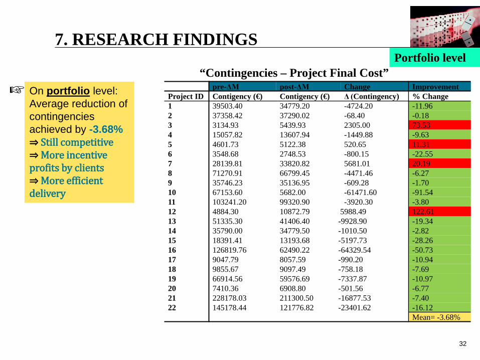
pre-ΔΜ post-ΔΜ Change Improvement Project ID Contigency (€) Contigency (€) Δ (Contingency) % Change 1 39503.40 34779.20 -4724.20 -11.96 2 37358.42 37290.02 -68.40 -0.18 3 3134.93 5439.93 2305.00 73.53 4 15057.82 13607.94 -1449.88 -9.63 5 4601.73 5122.38 520.65 11.31 6 3548.68 2748.53 -800.15 -22.55 7 28139.81 33820.82 5681.01 20.19 8 71270.91 66799.45 -4471.46 -6.27 9 35746.23 35136.95 -609.28 -1.70 10 67153.60 5682.00 -61471.60 -91.54 11 103241.20 99320.90 -3920.30 -3.80 12 4884.30 10872.79 5988.49 122.61 13 51335.30 41406.40 -9928.90 -19.34 14 35790.00 34779.50 -1010.50 -2.82 15 18391.41 13193.68 -5197.73 -28.26 16 126819.76 62490.22 -64329.54 -50.73 17 9047.79 8057.59 -990.20 -10.94 18 9855.67 9097.49 -758.18 -7.69 19 66914.56 59576.69 -7337.87 -10.97 20 7410.36 6908.80 -501.56 -6.77 21 228178.03 211300.50 -16877.53 -7.40 22 145178.44 121776.82 -23401.62 -16.12

Mean= -3.68%

On portfolio level: Average reduction of contingencies achieved by -3.68% ⇒ Still competitive ⇒ More incentive profits by clients ⇒ More efficient delivery

7. RESEARCH FINDINGS

“Contingencies – Project Final Cost” Portfolio level

29-04-2015 33

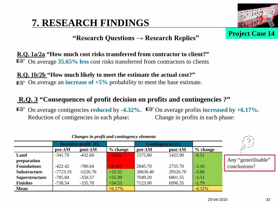
“Research Questions → Research Replies” R.Q. 1a/2a “How much cost risks transferred from contractor to client?”

On average 35.65% less cost risks transferred from contractors to clients R.Q. 1b/2b “How much likely to meet the estimate the actual cost?”

On average an increase of +5% probability to meet the base estimate.

R.Q. 3 “Consequences of profit decision on profits and contingencies ?”

On average contigencies reduced by -4.32%. Reduction of contigencies in each phase:

On average profits increased by +6.17%. Change in profits in each phase:


Incentive profit (€) Contingencies (€) pre-ΔΜ post-ΔΜ % change pre-ΔΜ post-ΔΜ % change

Land preparation

-341.79 -432.69 -26.60 1575.80 1425.90 -9.51

Foundations -422.42 -780.64 -84.80 2845.70 2755.70 -3.16 Substructure -7723.19 -5226.76 +32.32 30630.40 29526.70 -3.60 Superstructure -785.84 -350.57 +55.39 7049.20 6801.55 -3.51 Finishes -738.54 -335.78 +54.53 7123.90 6996.35 -1.79 Mean +6.17% -4.32%

Changes in profit and contingency elements

Any “generilisable” conclusions?

29-04-2015 34

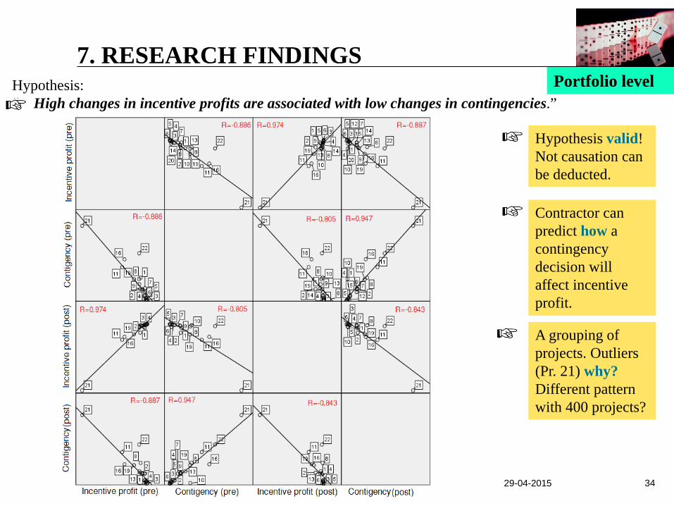
7. RESEARCH FINDINGS Portfolio level Hypothesis:

“ High changes in incentive profits are associated with low changes in contingencies.”

Hypothesis valid! Not causation can be deducted.

Contractor can predict how a contingency decision will affect incentive profit.

A grouping of projects. Outliers (Pr. 21) why? Different pattern with 400 projects?

29-04-2015 35

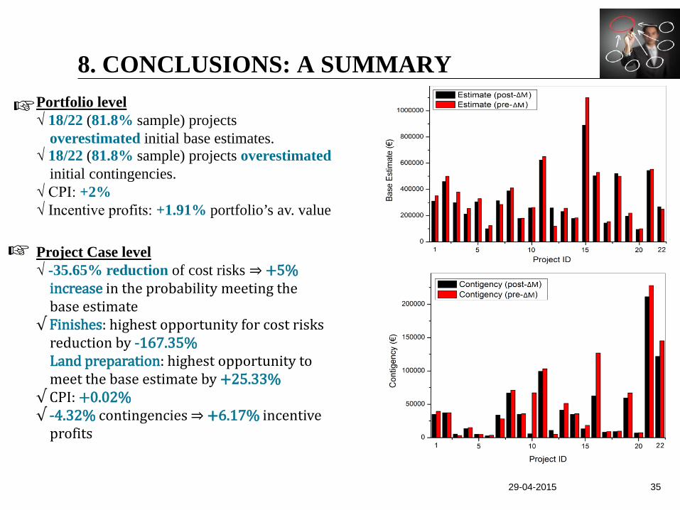
8. CONCLUSIONS: A SUMMARY Portfolio level √ 18/22 (81.8% sample) projects

overestimated initial base estimates. √ 18/22 (81.8% sample) projects overestimated

initial contingencies. √ CPI: +2% √ Incentive profits: +1.91% portfolio’s av. value

Project Case level √ -35.65% reduction of cost risks ⇒ +5%

increase in the probability meeting the base estimate

√ Finishes: highest opportunity for cost risks reduction by -167.35% Land preparation: highest opportunity to meet the base estimate by +25.33%

√ CPI: +0.02% √ -4.32% contingencies ⇒ +6.17% incentive

profits

29-04-2015 36

9. LIMITATIONS & FURTHER WORK “Limitations” ■ Sample → 35 questionnaires sent, 22 valid received: small sample ■ Industry

▪ Structure: fragmented with many SMEs ▪ Contractors: based too much on cost control accounting tools, not on RM systems ▪ Nature: legal framework very rigid and in favor of clients ▪ Decreasing profitability path

■ AHP scale → Linear scale selected ■ No validation and verification of cost risk analysis model

“Further work” ■ Pseudo-code integration into @RISK for optimal

contingency setting. ■ Client recommendation with a bidding proposal.

29-04-2015 37

“Client recommendation”

(Touran 2003)

Poisson distribution for cost risks

Contingency calculation for desired p(%)

Bid also for: √ T √ max. α √ max. χ → public (database)

→ private (consultant) √ agree post-bid on p Calculate Cch

Compare contingencies within the legal range

8. LIMITATIONS & FURTHER WORK

“Pseudo construction”

29-04-2015 38

MSc. Construction Management & Engineering Ir. Dimitrios Kordas Tel.: +31 649 177 841 E-mail: [email protected]

risk sharing in traditional construction contracts for building projects

Economy & Finance