RISK MANAGEMENT AT INSURANCE COMPANIES

PROFIT SHARING PRODUCTS

By

J.J.P. van Gulick

A Thesis

Submitted in partial fulfillment of the requirements for thedegree of

MASTER OF SCIENCE

(Business Mathematics & Informatics)

Vrije Universiteit Amsterdam

2012

c© 2012 J.J.P. van Gulick

This thesis, "Risk Management at Insurance Companies; Profit Sharing Products" is hereby

approved in partial fulfillment of the requirements for the Degree ofMaster of Sciencein Business

Mathematics & Informatics.

VU University AmsterdamFaculty of Exact Sciences

August 3, 2012

Signatures:

Thesis AdvisorDr. M. Boes

Thesis Co-AdvisorProf. Dr. G. M. Koole

Risk Management at Insurance CompaniesProfit Sharing Products

Van Gulick, J.J.P.

August 2012

VU University Amsterdam

Faculty of Exact Sciences

Business Mathematics & Informatics

De Boelelaan 1081a

1081 HV Amsterdam

Supervisors

Cardano Risk Management VU University

1. Van Antwerpen, V. 1. Dr. Boes, M.

2. Vermeijden, N. 2. Prof. Dr. Koole, G.M.

Abstract

This thesis gives a comprehensive analysis of typical profitsharing products sold in the Dutch life insurance

industry. The dynamics and parameters that influence the value of the product are revealed using replicating

portfolios consisting of swaptions. An alternative model,which explicitly considers sensitivity towards the

government curve and the euro swap curve, is introduced for this. This model provides additional insights,

as not modeling exposure to credit risk can have severe consequences in the valuation of these products and

consequently also in the construction of risk mitigating strategies. Therefore, this study considers several

hedge strategies that try to capture this exposure by including Credit Default Swap (CDS) contracts. Results

show that these strategies perform well but, because the payoff structure of these contracts remains linear,

do not completely capture the optional element in profit sharing products for extreme movements in the

credit spread. Not considering exposure to credit spread results in a hedge that only performs well when the

government curve and the swap curve move in equal direction simultaneously, but severely under performs

when this is not the case.

Keywords: Profit sharing, embedded options, life insurance, replicating portfolio, guaranteed returns, hedge strategies,

BPV, credit risk, credit default swap.

Preface

This thesis is written accompanying an internship that is anintegral part of the Business

Mathematics & Informatics Master program at VU University Amsterdam. The purpose of this

internship is to perform research on a practical problem individually during six months. The

problem and methods used should display all elements of the program, i.e., practical relevance to

the industry, mathematical modeling and computer science.This thesis is written at Cardano Risk

Management, a company that specializes in risk management using derivative overlay structures.

I would like to thank Mark-Jan Boes, for the supervision and feedback on this report. In the same

way I thank Ger Koole for his comments as involved second reader.

Special thanks go out to my two supervisors at Cardano, Vincent van Antwerpen and Niels

Vermeijden, for their continuous guidance and support during the internship. Finally, I would

like to thank Cardano as a whole for providing the internshipand therefore the opportunity to

graduate, and all colleagues there for contributing to an environment and atmosphere that helped

me considerably.

The subject of this thesis, and therefore also theory and terminology used, is finance related.

Because the program Business Mathematics & Informatics does not require comprehensive

knowledge of all this terminology, but everybody from this program should be able to understand

this thesis, a short description of the most important termsis given in the appendix. These terms

are formatteditalic when they are first introduced.

Jos van Gulick

Rotterdam, August 2012

v

Contents

Abstract . . . . . . . . . . . . . . . . . . . . . . . . . . . . . . . . . . . . . . . . . . . . . iii

Preface . . . . . . . . . . . . . . . . . . . . . . . . . . . . . . . . . . . . . . . . . . . . . v

Introduction . . . . . . . . . . . . . . . . . . . . . . . . . . . . . . . . . . . . . . . . . . 1

1 Profit Sharing Products . . . . . . . . . . . . . . . . . . . . . . . . . . . . . . . . . . 5

1.1 The position of profit sharing products within the Dutch pension system . . . . . . 6

1.2 Product specification . . . . . . . . . . . . . . . . . . . . . . . . . . . . .. . . . 7

1.3 U-yield . . . . . . . . . . . . . . . . . . . . . . . . . . . . . . . . . . . . . . . . 8

1.4 An example . . . . . . . . . . . . . . . . . . . . . . . . . . . . . . . . . . . . . . 9

1.5 Valuation of product sharing products . . . . . . . . . . . . . . .. . . . . . . . . 12

1.6 Some standard profit sharing products . . . . . . . . . . . . . . . .. . . . . . . . 17

1.6.1 Company A . . . . . . . . . . . . . . . . . . . . . . . . . . . . . . . . . . 18

1.6.2 Company B . . . . . . . . . . . . . . . . . . . . . . . . . . . . . . . . . . 24

1.7 Summary . . . . . . . . . . . . . . . . . . . . . . . . . . . . . . . . . . . . . . . 27

2 Risks . . . . . . . . . . . . . . . . . . . . . . . . . . . . . . . . . . . . . . . . . . . .29

2.1 Interest rate risk . . . . . . . . . . . . . . . . . . . . . . . . . . . . . . . .. . . . 29

2.2 Valuation and Swap-Government spread . . . . . . . . . . . . . . .. . . . . . . . 32

2.2.1 Swaps, Swaprates and Swaptions . . . . . . . . . . . . . . . . . . .. . . 33

2.2.2 Modeling government interest rate based swaptions . .. . . . . . . . . . 34

2.2.3 Model evaluation . . . . . . . . . . . . . . . . . . . . . . . . . . . . . . .38

2.2.4 A practical implementation . . . . . . . . . . . . . . . . . . . . . .. . . . 41

2.3 Summary . . . . . . . . . . . . . . . . . . . . . . . . . . . . . . . . . . . . . . . 49

3 Hedging strategies . . . . . . . . . . . . . . . . . . . . . . . . . . . . . . . . . . . . . 50

3.1 Framework . . . . . . . . . . . . . . . . . . . . . . . . . . . . . . . . . . . . . . 51

3.2 Instruments & Strategies . . . . . . . . . . . . . . . . . . . . . . . . . .. . . . . 52

3.2.1 Delta hedging . . . . . . . . . . . . . . . . . . . . . . . . . . . . . . . . . 53

vii

3.2.2 Delta hedging and CDS . . . . . . . . . . . . . . . . . . . . . . . . . . . .54

3.2.2.1 Credit Default Swap . . . . . . . . . . . . . . . . . . . . . . . . 54

3.2.3 Static Swaption and CDS hedge . . . . . . . . . . . . . . . . . . . . .. . 58

3.2.4 Linear and non-linear hedge portfolios ignoring swap-government spread . 59

3.3 Performance evaluation . . . . . . . . . . . . . . . . . . . . . . . . . . .. . . . . 59

3.3.1 Instantaneous performance . . . . . . . . . . . . . . . . . . . . . .. . . . 59

3.3.1.1 Delta Hedging . . . . . . . . . . . . . . . . . . . . . . . . . . . 60

3.3.1.2 Delta Hedging and CDS . . . . . . . . . . . . . . . . . . . . . . 60

3.3.1.3 Static Swaption hedge and CDS . . . . . . . . . . . . . . . . . . 61

3.3.1.4 Comparison . . . . . . . . . . . . . . . . . . . . . . . . . . . . 62

3.3.2 Performance over time . . . . . . . . . . . . . . . . . . . . . . . . . . .. 65

3.3.2.1 Scenario A . . . . . . . . . . . . . . . . . . . . . . . . . . . . . 66

3.3.2.2 Scenario B . . . . . . . . . . . . . . . . . . . . . . . . . . . . . 66

3.3.2.3 Scenario C . . . . . . . . . . . . . . . . . . . . . . . . . . . . . 67

3.3.2.4 Scenario D . . . . . . . . . . . . . . . . . . . . . . . . . . . . . 68

3.3.2.5 Comparison . . . . . . . . . . . . . . . . . . . . . . . . . . . . 69

3.4 A practical implementation . . . . . . . . . . . . . . . . . . . . . . . .. . . . . . 71

3.5 Summary . . . . . . . . . . . . . . . . . . . . . . . . . . . . . . . . . . . . . . . 73

Conclusion . . . . . . . . . . . . . . . . . . . . . . . . . . . . . . . . . . . . . . . . . . . 74

References . . . . . . . . . . . . . . . . . . . . . . . . . . . . . . . . . . . . . . . . . . . 77

A . . . . . . . . . . . . . . . . . . . . . . . . . . . . . . . . . . . . . . . . . . . . . . . .79

A.1 Function descriptions . . . . . . . . . . . . . . . . . . . . . . . . . . . .. . . . . 79

A.1.1 Profit sharing function . . . . . . . . . . . . . . . . . . . . . . . . . .. . 79

A.1.1.1 Input and parameters . . . . . . . . . . . . . . . . . . . . . . . . 80

A.1.1.2 Calculations . . . . . . . . . . . . . . . . . . . . . . . . . . . . 81

A.1.2 Hedge evaluation function . . . . . . . . . . . . . . . . . . . . . . .. . . 87

A.1.2.1 Input and parameters . . . . . . . . . . . . . . . . . . . . . . . . 87

A.1.2.2 Calculations . . . . . . . . . . . . . . . . . . . . . . . . . . . . 88

A.2 Financial products . . . . . . . . . . . . . . . . . . . . . . . . . . . . . . .. . . . 88

A.2.1 Option . . . . . . . . . . . . . . . . . . . . . . . . . . . . . . . . . . . . . 88

A.2.2 Swap . . . . . . . . . . . . . . . . . . . . . . . . . . . . . . . . . . . . . 89

A.2.3 Swaption . . . . . . . . . . . . . . . . . . . . . . . . . . . . . . . . . . . 89

A.3 Terminology . . . . . . . . . . . . . . . . . . . . . . . . . . . . . . . . . . . . .. 89

viii

Introduction

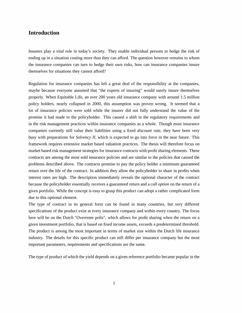
Insurers play a vital role in today’s society. They enable individual persons to hedge the risk of

ending up in a situation costing more than they can afford. The question however remains to whom

the insurance companies can turn to hedge their own risks, how can insurance companies insure

themselves for situations they cannot afford?

Regulation for insurance companies has left a great deal of the responsibility at the companies,

maybe because everyone assumed that "the experts of insuring" would surely insure themselves

properly. When Equitable Life, an over 200 years old insurance company with around 1.5 million

policy holders, nearly collapsed in 2000, this assumption was proven wrong. It seemed that a

lot of insurance policies were sold while the insurer did notfully understand the value of the

promise it had made to the policyholder. This caused a shift in the regulatory requirements and

in the risk management practices within insurance companies as a whole. Though most insurance

companies currently still value their liabilities using a fixed discount rate, they have been very

busy with preparations forSolvency II, which is expected to go into force in the near future. This

framework requires extensive market based valuation practices. The thesis will therefore focus on

market based risk management strategies for insurance contracts with profit sharing elements. These

contracts are among the most sold insurance policies and aresimilar to the policies that caused the

problems described above. The contracts promise to pay the policy holder a minimum guaranteed

return over the life of the contract. In addition they allow the policyholder to share in profits when

interest rates are high. The description immediately reveals the optional character of the contract

because the policyholder essentially receives a guaranteed return and acall optionon the return of a

given portfolio. While the concept is easy to grasp this product can adopt a rather complicated form

due to this optional element.

The type of contract in its general form can be found in many countries, but very different

specifications of the product exist at every insurance company and within every country. The focus

here will be on the Dutch "Overrente polis", which allows forprofit sharing when the return on a

given investment portfolio, that is based on fixed income assets, exceeds a predetermined threshold.

The product is among the most important in terms of market size within the Dutch life insurance

industry. The details for this specific product can still differ per insurance company but the most

important parameters, requirements and specifications arethe same.

The type of product of which the yield depends on a given reference portfolio became popular in the

1

eighties1 when rising interest rates led to a significant flow of capitalinto financial markets. This,

in turn, resulted in increased competition between financial institutions, forcing also life insurance

companies to sell products with a higher yield, making them more sensitive to interest rate changes.

Equitable life was not the first insurer to get into trouble, already in the late eighties some life

insurance companies got insolvent with many more to follow.The main reason was that these

products had always been considered very safe because the low guaranteed rate represented an

option with astrike very far out of the money. When interest rates fell sharply at the start of the

nineties, the first problems however arose quickly.

These circumstances sparked an amount of academic research, focusing mainly onunit- and equity

linked productsat first. Because these products give a return that is directly linked to the return on

a given reference portfolio, they are generally easier to understand and to value than most profit

sharing products including a guaranteed return.

Around the year 2000, the risks from the optional character in profit sharing products became

apparent as several companies had to file for bankruptcy as a direct consequence of it. This caused an

emergence of academic literature and regulatory reforms. Among the first to address the valuation of

the optional character were Briys and de Varenne (1994),Hipp (1996),Miltersen and Persson (2000)

and Grosen and Jorgensen (2000). Research in the following years contributed to the ideas from

these authors by including mortality and surrender options, but also by addressing issues more

specific to insurance policies sold in different countries.This has led to a substantial amount

of literature on the fair valuation of contracts that are sold in several countries, including the

Netherlands. The first to address the problem of guaranteed returns offered by Dutch insurance

companies was Donselaar (1999). He showed that the demand for these products quickly rose

during the nineties when they started to be used as pension plans as well. But also that most insurers

probably did not charge enough for the products they sold andthat they were likely to use investment

strategies that did not match with their liabilities, exposing them to risks. Bouwknegt and Pelsser

(2001) used the optional character of a simple profit sharingproduct and came up with a fair

valuation based on a replicating portfolio. Later, Plat andPelsser (2008) found an analytical

expression for the fair value of a profit sharing product thatcan be considered as a type of "Overrente

polis".

It is clear from the above that quite some research has been done on the fair valuation of a wide

range of insurance policies with embedded options during the last two decades. However, little

attention has gone to the risks involved with these contracts and possible hedge strategies. Some

basic elements have been discussed but they are mainly theoretical, as they are often a result of the

replicating portfolios used in the valuation.

1The first form of a with profit sharing product was sold alreadyin 1806 according to Sibbett (1996).

2

Because the profit sharing of the "Overrente polis" is determined by a complex yield that is based on

Dutch government bonds, the swap rate is often taken as an approximation to simplify calculations.

This can lead to problems in modeling these products and in the construction of risk mitigating

strategies. An important contribution to existing literature lies in the reevaluation of this assumption.

For this an alternative model is introduced that quantifies these risks, provides additional insights

and allows for the construction of strategies and testing environments that should be more effective.

The aim of this work is to create understanding in the value and dynamics of typical profit sharing

products. Questions that will be answered are:a) How can the fair value of the product be

computed?;b) What factors influence the value of the profit sharing?; andc) What approach can be

taken to mitigate the risks that these factors introduce?

In summary the results of this thesis show that a replicatingportfolio of swaptions and a zero

coupon bond can estimate the fair value of these contracts consistently. The value of these swaptions

should however be computed by explicitly considering sensitivity towards a government curve and

a discount curve.

Neglecting sensitivity towards country credit risk can result in significant modeling errors and the

construction of weak performing hedge strategies, as the credit risk premium can cause strong

fluctuations in the value of these products.

The long maturity of these contracts, liquidity issues and laws prohibiting short selling of

government debt, impose limitations in the construction ofeffective hedge strategies that incorporate

exposure to credit risk. The use of CDS contracts in this however seems to be an effective alternative.

Furthermore, the results in this paper strongly suggest that the fair value of these contracts is

significantly higher than the price for which they can be bought.

The remainder of this thesis will have the following structure. Chapter 1 will describe the profit

sharing product in general. First the position of the profit sharing product within the Dutch pension

and insurance system will be drawn. In the subsequent section the most popular type of profit

sharing product sold in the Netherlands is discussed and an example will be provided. Next, it will

be shown how a replicating portfolio can be constructed which is consistent with precise contract

specifications. With this, the value and the sensitivity of these products at a given moment in time

can be estimated. At the end of the first chapter two products with alternative structures that are

often encountered will be considered and the results from the earlier sections will be applied.

In chapter 2 the results of the first chapter will be used to determine the risks that these contracts

introduce to the books of the insurance company. Several risks will be analyzed for different

scenarios and methods that can help mitigating these risks will be discussed. A model that considers

exposure to credit risk will be introduced and evaluated. Both the dynamics of the guarantee and

3

the profit sharing will be analyzed.

Several risk mitigating strategies will be discussed in more detail in chapter 3, where special

attention is given to the practical implementability of thesuggested hedging strategies, as the

findings of this thesis are meant to provide methods that workand can readily be applied in the

daily operations of risk managers. This chapter will describe products and strategies that can be

used. The effectiveness of these strategies will also be assessed for several scenarios. Special

attention here will be given to the use of CDS contracts in hedging the exposure to country credit

risk.

The last chapter concludes.

4

Chapter 1

Profit Sharing Products

There is profit sharing in a number of products, organizations and industries. The type of profit

sharing discussed here stems from a product which is a form ofdefined benefit pension plan offered

by insurance companies, together withunit-linked products. The profit sharing products mainly

differ from unit-linked products in that the return is not directly linked to some reference portfolio

which can be chosen by the policyholder to match his risk appetite. Instead the return on profit

sharing products is typically based on a predefined, fictive,investment policy. Though unit-linked

products generally also offer some kind of minimum rate of return guarantee (MRRG), by promising

a fixed amount at expiration of the contract, it is lower than in a typical profit sharing contract and

the policyholder bears a much larger part of the risks.

The motivation behind profit sharing products is twofold. First, it should provide a stable return to

the policyholder, with low risk through the minimum return guarantee while still being competitive

with other financial assets through the profit sharing. Secondly, the smoothing of returns by the

investment policy, that on the one hand provides stable returns for the policyholder, should also

ensure less volatile market values of the liabilities.

This chapter will begin by shortly discussing the function and position of the profit sharing product

in society. In section 1.2 a precise specification of a Dutch profit sharing contract, the "Overrente

polis", will be given. Section 1.3 will discuss the so calledu-yield, a rate that is used to determine the

bulk of Dutch profit sharing products. In section 1.5 an efficient and consistent way to value these

products by the use of a replicating portfolio will be given.Using this valuation some important

properties and sensitivities will be addressed. Finally the results will be applied to two contracts of

known form in section 1.6.

5

1.1 The position of profit sharing products within the Dutch pension

system

The Dutch pension system is based on three pillars:

1. A state pension that every citizen receives after the age of 65. It is linked to the statutory

mimimum wage and provides a minimum income to prevent real poverty. This pillar is based

on a pay as you go framework, meaning that the people currently having a job provide for

the retirees, and is a result of two acts; 1) The general Old Age Pensions Act [Algemene

Ouderdomswet(AOW)], that came into force in 1957 and 2) the National Survivor Benefits

Act [Algemene Nabestaandenwet(ANW)].

2. A supplementary pension build up during the working life of a citizen. This pillar is, as it is

in other countries, still a crucial one for the citizen to enjoy a decent pension after retiring.

It consists of collective pension schemes that are administered by either a pension fund or an

insurance company. Because membership of a pension fund is mandatory for many sectors

and professions, today about 94% of the employees belong to apension fund, of which there

were 514 (end 2010). There are three different types of pension funds:

- Corporate pension funds (for one single company or corporation).

- Industry-wide pension funds (for all employees of a whole sector).

- Pension funds for independent professionals.1

These pension funds are non-profit and strictly separated from the companies. Therefore

financial trouble for the company will not directly effect the pension plans of the employees.

The pension plans are financed by capital funding. Meaning that they are paid for by

contributions and returns on investments made by the funds.Today the managed capital of

all Dutch pension funds amounts to overe 746 billion, exceeding the dutch GDP by about

26%.

3. The third pillar consists of individual pension products. It is used by employees not

participating in a collective pension scheme or people thatprefer a more assuring pension

plan in addition to the second pillar. Utilizing savings forthe purpose of a pension one can

often take advantage of tax benefits.

1For example pilots, dentist and doctors all have separatelymanaged pension plans.

6

Profit sharing products can be placed in either the second or the third pillar when a person buys such

a product at a insurance company through his or her employer or individually. In a less obvious way

they are also used indirectly by pensions funds and insurance companies through reassurance. A

companies pension fund with defined benefit pension contracts might want to transfer some of the

risk by use of a profit sharing product sold by an insurance company.

1.2 Product specification

In the contract of a profit sharing product the insurer usually promises to pay a fixed amount to the

policyholder in the future. This amount is then either discounted using a fixed interest rate, called

the technical rate or the guaranteed raterg, and paid as a lump sum at inception of the contract or

paid by regular premiums over the life of the contract.

Every year the reserve of the account the policyholder has atthe insurer grows by the guaranteed

rate but the policyholder also has an option, representing the profit share, on the return of some

investment portfolio the insurer manages according to a predetermined policy. Often the profit

sharing returnrPS is also subject to a certain participation levelα and/or feeδ subtracted before the

sharing. The profit sharing return can then be defined as

rPS= maxα[

r f i − (rg+δ ),0]

, (1.1)

with r f i the return on the investment portfolio, which is often defined by a fictive investment policy,

hencef i. This portfolio should not be confused with how the insurance company actually manages

its assets and is only used for the determination of the profitsharing rate. Becauser f i is the only

parameter that varies each period in equation 1.1, this is the most important element in the valuation

of the profit sharing part of this product and it ensures the stable and smoothed returns discussed

earlier. The investment policy can differ substantially between insurance companies but is mostly

based on fictitious investments in the u-rate. This is a weighted average yield on a number of

bonds issued by the Dutch state and will be discussed in more detail later. The use of the u-rate

is the first step in smoothing returns as it is a weighted average of a number of underlying yields.

To stabilize the profit sharing further, a weighted average return on the investments made against

different u-rates in the fictive portfolio is used, settingr f i equal to the return on a portfolio of fixed

income products.

For a product that pays out the profit sharing component each year and a fictive portfolio that invests

in M year bonds the above can be summarized by the following steps.

7

At the start of the year the premium, the coupons from previous investments and possible

redemptions are received. This amount is then invested in bonds yielding the then prevailing u-rate

with a fixed maturity ofM years and a fixed turnover structure. At the end of the year theweighted

return on all investments made up to then can be computed by considering all coupons. Based on

this return the amount of profit sharing can be determined.

Essentially it is a simple idea and this is why insurers promote it as being perfectly transparent.

This structure will however cause some difficulties in determining efficient hedging strategies and

consistent valuation.

Based on the above a contract that pays out the profit sharing every year is defined by:

1. CFi The cash flow to be paid to the policyholder in yeari, the horizon.

2. rg The minimum guaranteed rate of return.

3. M Maturity of assets in the reinvestment strategy.

4. T A turnover structure of the investments.

5. δ The fee subtracted from the profit sharing.

6. α The participation level of the policyholder in the profit sharing.

To give some more insight in how the profit sharing evolves an example will be given in section 1.4.

1.3 U-yield

The profit sharing rates of European life insurance contracts are most often based on the return

of a reference portfolio containing fictitious fixed income assets. In the Netherlands it is common

practice to invest in fixed income products that have a rate that is based on bonds issued by the

Dutch state. Three yields are used in the Dutch life insurance industry for this purpose; the s-yield,

the t-yield and the u-yield. All yields are computed in a similar complicated way where the s-yield

computes a yield that is corrected for inflation compared to the t-yield and u-yield. The main

difference between the latter two is that the t-yield considers bonds with a longer maturity, i.e., it

includes maturities from 7 years on (except perpetual bonds). All yields are published by "Verbond

van Verzekeraars", a Dutch association of insurance companies. The u-yield is by far the most

popular yield, hence this will be the one discussed here.

8

Definition of the u-yield.

The u-yield is determined every15th of the month as the average yield on 6 past "part" yields,

computed at the same time as a weighted2 average of medians of yields over different maturity

segments of all bonds issued by the Dutch state that have a principal of at leaste 255 mln and a

remaining maturity between 2 and 15 years.3

The above definition makes clear that this rate has been setupin a way that makes any computation

of a valuation or projection of the profit sharing at the leastvery inefficient, if not impossible.

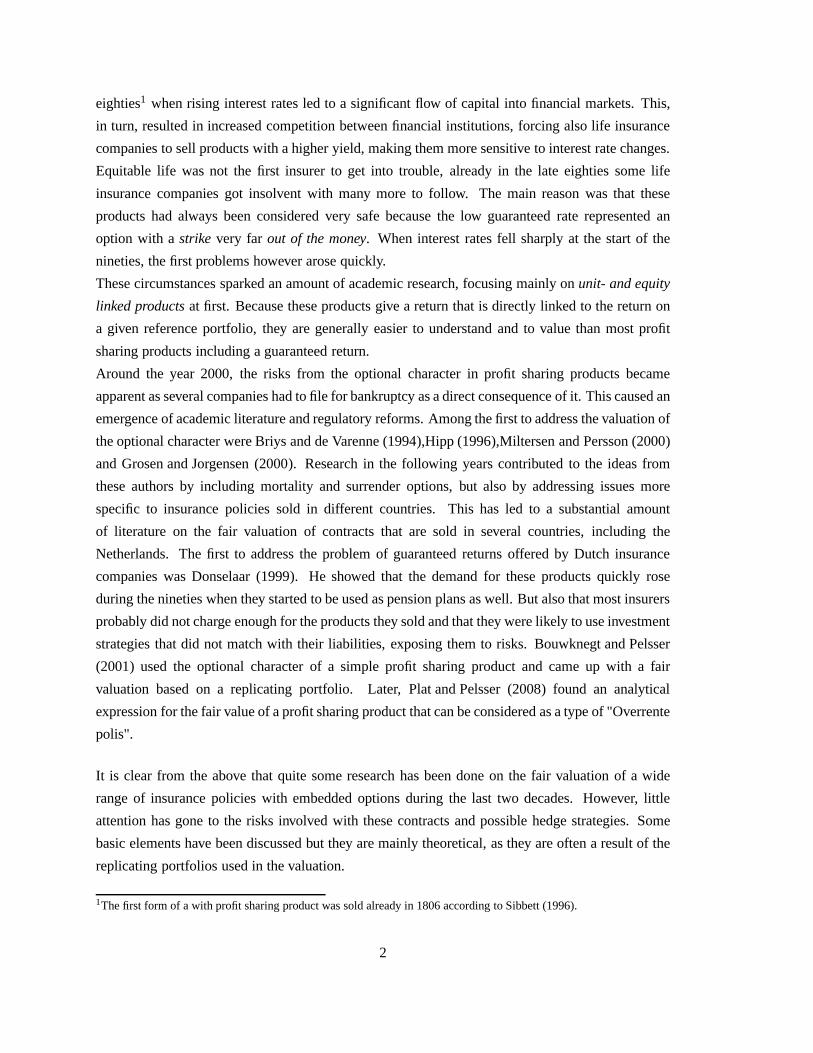
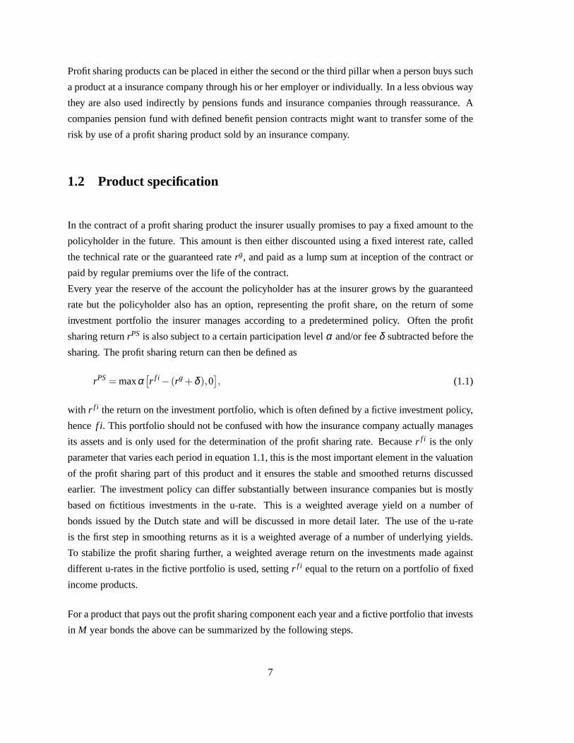
Because of this a proxy is often used for computations requiring the u-rate. From historical data the

7-year swap rate has been known to be a good proxy (see figure 1.1).

Earlier literature does not elaborate on possible reasons why this is a good proxy and start

calculations based on the 7 year swaprate right away. One thing that is obvious from the figure

is that the 7 year swap rate is more volatile than the u-rate, what makes sense since the latter is an

averaged value. This mismatch will cause differences in thevaluation of the embedded option.

For now the 7 year swap rate will be taken as basis for projections of the u-rate as this is the best

indicator at hand. Later, in section 2.2.2, the risks implied by making this assumption will be

discussed.

It should also be clear that, though the 7 year swap rate is a good proxy for the u-yield, this does not

mean it is a good proxy for the profit sharing rate as this rate crucially depends on the investment

policy and timing of the reference portfolio.

1.4 An example

To give some more insight into how the profit sharing is determined, how the investment portfolio

and reserve are related, and how they evolve over time a simple example is worked out in this

section.

Consider a contract that payse 100 mln in 30 years with a guaranteed interest rate of 1.0%, a

reinvestment strategy in coupon bonds with a maturity of 7 years and a yield equal to the u-yield

prevailing in that period, no fee, 100% participation and ispaid by one lump sum at inception of the

2This weighing scheme is not based on the principals but on fixed percentages that depend on the maturity.3For a more precise definition of the u-yield, but also the t- and f-yield see:http://www.verzekeraars.nl/UserFiles/File/cijfers/Definitie%20rendementen%20s%20t%20u.pdf

9

2000 2001 2002 2003 2004 2005 2006 2007 2008 2009 2010 2011 2012

0.010

0.015

0.020

0.025

0.030

0.035

0.040

0.045

0.050

0.055

0.0607y swap U−yield

7y swap − 3 month MA

0 5 10 15 20 25

0.1

0.2

0.3

0.4

0.5

0.6

0.7

0.8

0.9

1.0ACF: 7y swap ACF: U−yield

ACF: 7y swap − 3 month MA

Variable min mean max σ

7y swap 0.0185 0.0392 0.0581 0.009687y swap - 3 month MA 0.0200 0.0394 0.0575 0.00902U-yield 0.0187 0.0386 0.0543 0.00864

Figure 1.1. This figure shows the 7 year swap rate as obtained from Bloomberg, its 3 month moving average,computed with 6 half month datapoints, and the u-yield over the period January 2000 to April 2012. In thebottom left the autocorrelations are displayed. The table in the bottom right displays some summary statisticsof these series.

contract. The return of this contract is computed in the following way:

t=0 The amount in the reserve and in the fictive investment portfolio managed by the insurer is

equal and computed using a discount factor based on the horizon of the cash flow and the

technical raterg

R0 = I0 = df iCF30 = (1+ rg)−30CF30 = e 74,192,292,

with R0 the reserve andI0 the amount in the investment portfolio at timet = 0. I0 is then

10

invested completely in a bond with a yieldu0, the prevailing u-yield att = 0, and has a

maturity of 7 years. At the end of the first period the return onthe fictive investment portfolio

equals the coupon from the bond. If the u-yield at inception wasu0 = 2.5%, the profit sharing

can be computed from equation 1.1 as

rPS0 = max

[

α(r f i0 − (rg+δ ),0

]

= max[2.5%−1.0%,0] = 1.5%.

This means that there is a profit sharing at the end of the period of

PS0 = 1.5%·R0 = 1.5%·e 74,192,292= e 1,112,884.

This amount would be paid out to the policyholder and only 1%< u0, equal to the increase

of the reserve, will be available for investment in the fictive portfolio. If u0 would have been

lower thenrg = 1% , the insurer would have to honor the contract and let the reserveR0

increase by the guaranteed rate of 1% toR1 = R0(1+ rg), while the investment portfolio

only grew byu0 < rg. Only u0 would then be available for investmentI1 at the beginning

of the next period, ensuring a lower likelihood for future profit sharing if u-rates will rise to

compensate the insurer becauseu0 will have a weight inr f ii for 7 years. As a consequence the

amount available for investment at the beginning of a periodis always based on min(r f it−1, r

g).

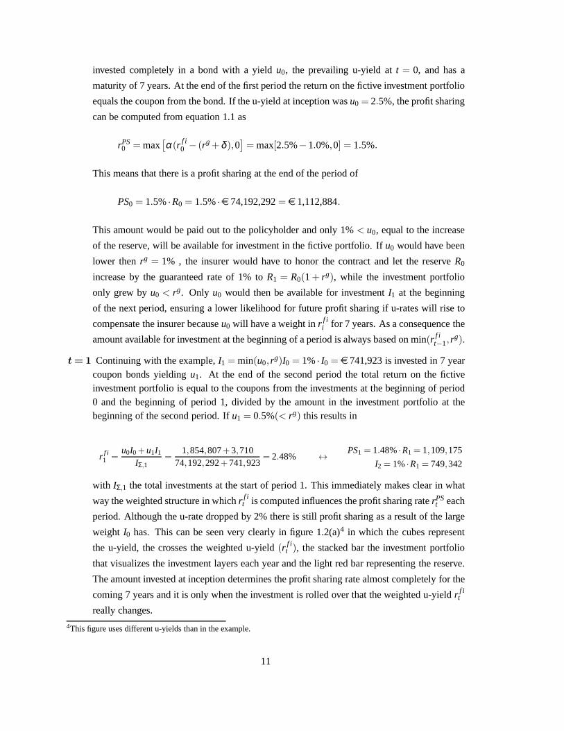
t=1 Continuing with the example,I1 = min(u0, rg)I0 = 1%· I0 = e 741,923 is invested in 7 yearcoupon bonds yieldingu1. At the end of the second period the total return on the fictiveinvestment portfolio is equal to the coupons from the investments at the beginning of period0 and the beginning of period 1, divided by the amount in the investment portfolio at thebeginning of the second period. Ifu1 = 0.5%(< rg) this results in

r f i1 =

u0I0+u1I1IΣ,1

=1,854,807+3,710

74,192,292+741,923= 2.48% ↔ PS1 = 1.48%·R1 = 1,109,175

I2 = 1%·R1 = 749,342

with IΣ,1 the total investments at the start of period 1. This immediately makes clear in what

way the weighted structure in whichr f it is computed influences the profit sharing raterPS

t each

period. Although the u-rate dropped by 2% there is still profit sharing as a result of the large

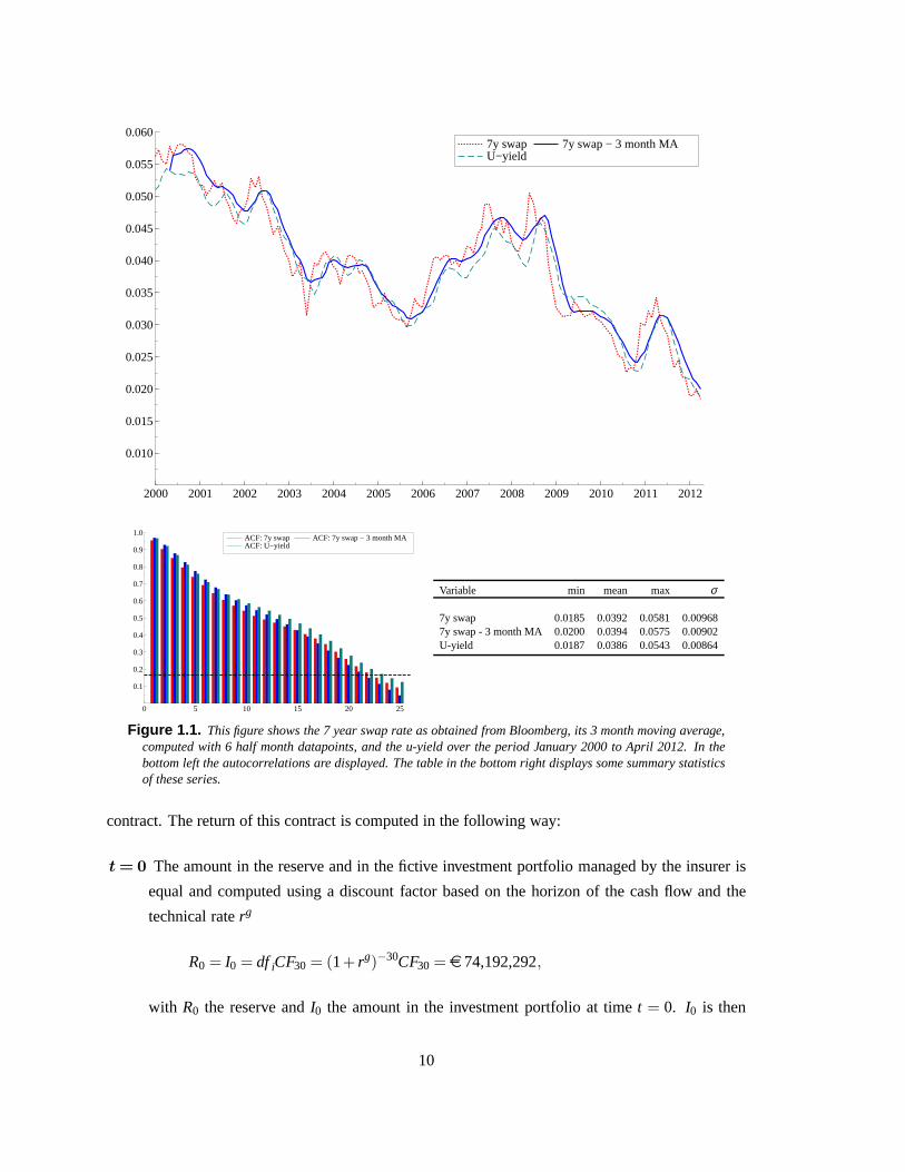
weight I0 has. This can be seen very clearly in figure 1.2(a)4 in which the cubes represent

the u-yield, the crosses the weighted u-yield(r f it ), the stacked bar the investment portfolio

that visualizes the investment layers each year and the light red bar representing the reserve.

The amount invested at inception determines the profit sharing rate almost completely for the

coming 7 years and it is only when the investment is rolled over that the weighted u-yieldr f it

really changes.

4This figure uses different u-yields than in the example.

11

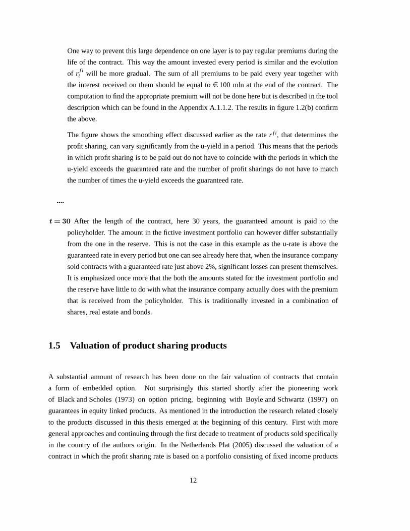
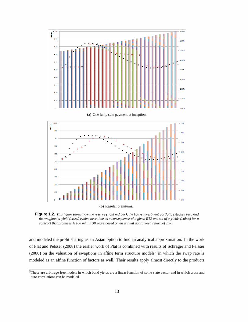
One way to prevent this large dependence on one layer is to payregular premiums during the

life of the contract. This way the amount invested every period is similar and the evolution

of r f it will be more gradual. The sum of all premiums to be paid every year together with

the interest received on them should be equal toe 100 mln at the end of the contract. The

computation to find the appropriate premium will not be done here but is described in the tool

description which can be found in the Appendix A.1.1.2. The results in figure 1.2(b) confirm

the above.

The figure shows the smoothing effect discussed earlier as the rater f i, that determines the

profit sharing, can vary significantly from the u-yield in a period. This means that the periods

in which profit sharing is to be paid out do not have to coincidewith the periods in which the

u-yield exceeds the guaranteed rate and the number of profit sharings do not have to match

the number of times the u-yield exceeds the guaranteed rate.

....

t=30 After the length of the contract, here 30 years, the guaranteed amount is paid to the

policyholder. The amount in the fictive investment portfolio can however differ substantially

from the one in the reserve. This is not the case in this example as the u-rate is above the

guaranteed rate in every period but one can see already here that, when the insurance company

sold contracts with a guaranteed rate just above 2%, significant losses can present themselves.

It is emphasized once more that the both the amounts stated for the investment portfolio and

the reserve have little to do with what the insurance companyactually does with the premium

that is received from the policyholder. This is traditionally invested in a combination of

shares, real estate and bonds.

1.5 Valuation of product sharing products

A substantial amount of research has been done on the fair valuation of contracts that contain

a form of embedded option. Not surprisingly this started shortly after the pioneering work

of Black and Scholes (1973) on option pricing, beginning with Boyle and Schwartz (1997) on

guarantees in equity linked products. As mentioned in the introduction the research related closely

to the products discussed in this thesis emerged at the beginning of this century. First with more

general approaches and continuing through the first decade to treatment of products sold specifically

in the country of the authors origin. In the Netherlands Plat(2005) discussed the valuation of a

contract in which the profit sharing rate is based on a portfolio consisting of fixed income products

12

(a) One lump sum payment at inception.

(b) Regular premiums.

Figure 1.2. This figure shows how the reserve (light red bar), the fictive investment portfolio (stacked bar) andthe weighted u-yield (cross) evolve over time as a consequence of a given RTS and set of u-yields (cubes) for acontract that promisese 100 mln in 30 years based on an annual guaranteed return of 1%.

and modeled the profit sharing as an Asian option to find an analytical approximation. In the work

of Plat and Pelsser (2008) the earlier work of Plat is combined with results of Schrager and Pelsser

(2006) on the valuation of swaptions in affine term structuremodels5 in which the swap rate is

modeled as an affine function of factors as well. Their results apply almost directly to the products

5These are arbitrage free models in which bond yields are a linear function of some state vector and in which cross andauto correlations can be modeled.

13

discussed in this thesis, though they will not be used here inthe sense that a precise analytical

formula is used for valuation. The structure used for the replication of the profit sharing part will

however be similar.

The value of the profit sharing will also be approximated by creating a replicating portfolio and

using the no-arbitrage argument that if the replicating portfolio has exactly the same cash flows as

the profit sharing their value should be the same. Otherwise ariskless profit can be made by selling

the one and buying the other.

The amount of profit sharing at the end of every periodi is a function of the variable return on the

fictive investment portfolio, the reserve at the beginning of the period, which is predetermined if the

profit sharing is to be paid out, a constant guaranteed rate, afee and a participation level:

PSi(rf ii ,Ri) = Ri max

[

r f ii − (rg+δ ),0

]

,

with Ri being the reserve at the beginning of periodi, rg the guaranteed rate andδ the fee, assuming

that the participationα is equal to 1.

r f ii , the return of the investment portfolio at the end of periodi, is a weighted function of the

investments done in previous periods. For most insurance policies sold in the Netherlandsr f ii would

then be

r f ii =

i

∑q=(i−M+1)+

uqIqIΣ,i

IΣ,i =i

∑q=(i−M+1)+

Iq, (1.2)

with M the maturity of the bonds,uq the u-yield at the beginning of periodq, Iq the amount invested

in periodq, often called a layer andIΣ,i the sum of all investments at the beginning of periodi. Iq,

the amount that can be invested every period, depends on the turnover structure of the investments

through the payments every period, the historical u-yieldswhich determine the coupons and the

premiums.

If r f ii would be an interest rate quoted in the market, this cash flow could be replicated by use of

a strip of Europeanswaptionson the interest rater f ii of which one expires every period and has a

strike rg+δ , anotional Ri and lasts one period. Using the distribution ofr f ii the value can then be

computed by use of standard option theory.

The fact thatr f ii is a return on investments driven by a specific investment policy, that these

investments have a yield that is itself a complex weighted average of yields and that the amount

in the reserve can depend on profit sharing if the profit share is reinvested each year, complicates

14

things.

First consider the simplified case in which the profit share ispaid out every period and the turnover

structure of the reinvestments specifies that the principalis paid back in full at maturity.

The element that is least straightforward but most crucial in modeling the replicating portfolio, as

to match the cash flows of the profit share as good a possible, isdetermining the notionals of the

swaptions. Intuivitively is it clear that these notionals should depend on the amount in the reserve,

because this is the amount over which the profit sharing rate is due at the end of every period, and

on the reinvestments at the beginning of the period, becausethis determines the weighting.

In the case the u-yield exceeds the guaranteed rate every period the weighing does not influence

the profit sharing as to it is paid out or not because there willbe profit sharing every period. The

notionals of the underlying swaptions are then known for every period as the amount in the reserve

Ri grows every year by a fixed raterg and this increase is equal to the reinvestment in the fictive

portfolio next period . The notionals for the swaptions every period are in this case therefore equal

to the amount available for investment in the fictive portfolio (return - profit sharing). The sum

of all cashflows from the underlyingswaps(swaptions are sure to endin the money) will now

exactly match the profit share because the notionals perfectly replicate the weighing scheme or

reinvestments.

However, in general the amount in the investment portfolio and the amount in the reserve will not

be equal. If the return on the fictitious investments in a period is below the guaranteed rate,r f ii < rg,

the reserve will grow faster than the fictive investment portfolio. If δ > 0 and 0< r f ii − rg < δ the

reserve will just grow byrg but the investments will grow byr f ii > rg. Therefore the investments

made every period by the investment portfolio, though they match the weighing part perfectly, can

not be used as notional for the swaptions.

The solution is that the notionals should be based on the reserve, as this is the amount that determines

the profit sharing together withr f i . To incorporate the weighting effect correctly the premiums paid

should be invested using the same policy as the fictive portfolio but based on the guaranteed raterg

instead of the u-yields.

Under the assumption that profit share is paid out every period and the turnover structure is just that

the principal is paid back in full at maturityM, the swaption notionalNi for period i is determined

by the recursive formula

Ni = Ni−M + rgi−1

∑q=(i−M)+

Nq = Ni−M + rgRi−1.

15

Assuming also that there is a good proxy for the u-yield, which seems to be a reasonable assumption

considering the analysis in the last subsection (see also 1.1), the value of the profit sharing element

at the start of periodt is then equal to the strip of swaptions

VPSt =

n

∑i=t

Vswaptiont,i (Ni,σui , r

g+δ ,M), (1.3)

with σuq theimplied volatilityof the u-yield proxy,rg+δ the strike,i the exercise date,M the length

of the underlying swap andn the horizon of the contract.6

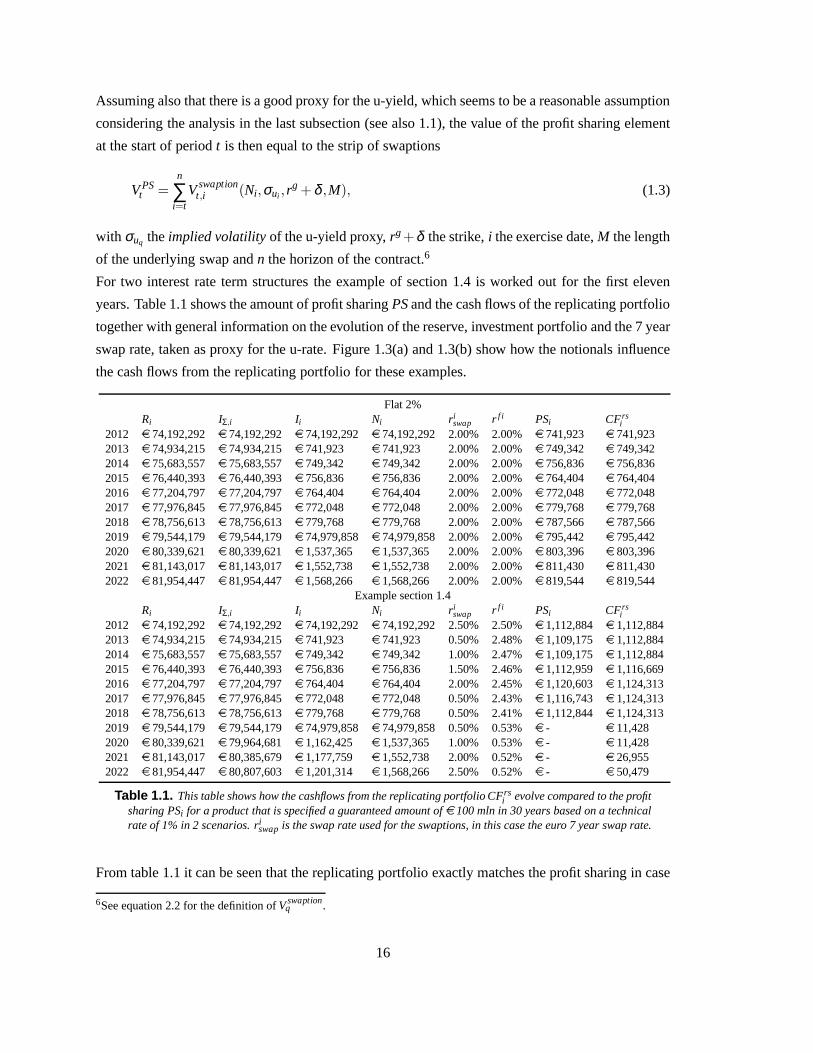
For two interest rate term structures the example of section1.4 is worked out for the first eleven

years. Table 1.1 shows the amount of profit sharingPSand the cash flows of the replicating portfolio

together with general information on the evolution of the reserve, investment portfolio and the 7 year

swap rate, taken as proxy for the u-rate. Figure 1.3(a) and 1.3(b) show how the notionals influence

the cash flows from the replicating portfolio for these examples.

Flat 2%Ri IΣ,i Ii Ni r i

swap r f i PSi CFrsi

2012 e 74,192,292 e 74,192,292 e 74,192,292 e 74,192,292 2.00% 2.00%e 741,923 e 741,9232013 e 74,934,215 e 74,934,215 e 741,923 e 741,923 2.00% 2.00% e 749,342 e 749,3422014 e 75,683,557 e 75,683,557 e 749,342 e 749,342 2.00% 2.00% e 756,836 e 756,8362015 e 76,440,393 e 76,440,393 e 756,836 e 756,836 2.00% 2.00% e 764,404 e 764,4042016 e 77,204,797 e 77,204,797 e 764,404 e 764,404 2.00% 2.00% e 772,048 e 772,0482017 e 77,976,845 e 77,976,845 e 772,048 e 772,048 2.00% 2.00% e 779,768 e 779,7682018 e 78,756,613 e 78,756,613 e 779,768 e 779,768 2.00% 2.00% e 787,566 e 787,5662019 e 79,544,179 e 79,544,179 e 74,979,858 e 74,979,858 2.00% 2.00%e 795,442 e 795,4422020 e 80,339,621 e 80,339,621 e 1,537,365 e 1,537,365 2.00% 2.00%e 803,396 e 803,3962021 e 81,143,017 e 81,143,017 e 1,552,738 e 1,552,738 2.00% 2.00%e 811,430 e 811,4302022 e 81,954,447 e 81,954,447 e 1,568,266 e 1,568,266 2.00% 2.00%e 819,544 e 819,544

Example section 1.4Ri IΣ,i Ii Ni r i

swap r f i PSi CFrsi

2012 e 74,192,292 e 74,192,292 e 74,192,292 e 74,192,292 2.50% 2.50%e 1,112,884 e 1,112,8842013 e 74,934,215 e 74,934,215 e 741,923 e 741,923 0.50% 2.48% e 1,109,175 e 1,112,8842014 e 75,683,557 e 75,683,557 e 749,342 e 749,342 1.00% 2.47% e 1,109,175 e 1,112,8842015 e 76,440,393 e 76,440,393 e 756,836 e 756,836 1.50% 2.46% e 1,112,959 e 1,116,6692016 e 77,204,797 e 77,204,797 e 764,404 e 764,404 2.00% 2.45% e 1,120,603 e 1,124,3132017 e 77,976,845 e 77,976,845 e 772,048 e 772,048 0.50% 2.43% e 1,116,743 e 1,124,3132018 e 78,756,613 e 78,756,613 e 779,768 e 779,768 0.50% 2.41% e 1,112,844 e 1,124,3132019 e 79,544,179 e 79,544,179 e 74,979,858 e 74,979,858 0.50% 0.53%e - e 11,4282020 e 80,339,621 e 79,964,681 e 1,162,425 e 1,537,365 1.00% 0.53%e - e 11,4282021 e 81,143,017 e 80,385,679 e 1,177,759 e 1,552,738 2.00% 0.52%e - e 26,9552022 e 81,954,447 e 80,807,603 e 1,201,314 e 1,568,266 2.50% 0.52%e - e 50,479

Table 1.1. This table shows how the cashflows from the replicating portfolio CFrsi evolve compared to the profit

sharing PSi for a product that is specified a guaranteed amount ofe 100 mln in 30 years based on a technicalrate of 1% in 2 scenarios. ri

swapis the swap rate used for the swaptions, in this case the euro 7year swap rate.

From table 1.1 it can be seen that the replicating portfolio exactly matches the profit sharing in case

6See equation 2.2 for the definition ofVswaptionq .

16

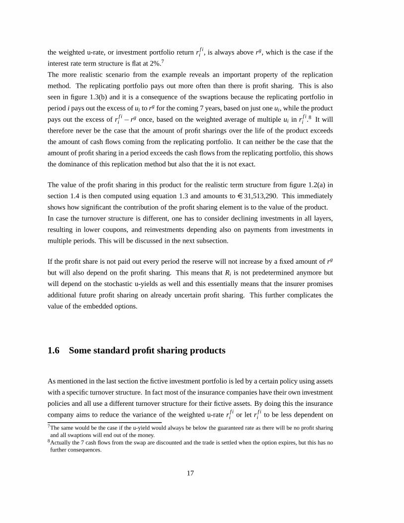
the weighted u-rate, or investment portfolio returnr f ii , is always aboverg, which is the case if the

interest rate term structure is flat at 2%.7

The more realistic scenario from the example reveals an important property of the replication

method. The replicating portfolio pays out more often than there is profit sharing. This is also

seen in figure 1.3(b) and it is a consequence of the swaptions because the replicating portfolio in

periodi pays out the excess ofui to rg for the coming 7 years, based on just oneui , while the product

pays out the excess ofr f ii − rg once, based on the weighted average of multipleui in r f i

i .8 It will

therefore never be the case that the amount of profit sharingsover the life of the product exceeds

the amount of cash flows coming from the replicating portfolio. It can neither be the case that the

amount of profit sharing in a period exceeds the cash flows fromthe replicating portfolio, this shows

the dominance of this replication method but also that the itis not exact.

The value of the profit sharing in this product for the realistic term structure from figure 1.2(a) in

section 1.4 is then computed using equation 1.3 and amounts to e 31,513,290. This immediately

shows how significant the contribution of the profit sharing element is to the value of the product.

In case the turnover structure is different, one has to consider declining investments in all layers,

resulting in lower coupons, and reinvestments depending also on payments from investments in

multiple periods. This will be discussed in the next subsection.

If the profit share is not paid out every period the reserve will not increase by a fixed amount ofrg

but will also depend on the profit sharing. This means thatRi is not predetermined anymore but

will depend on the stochastic u-yields as well and this essentially means that the insurer promises

additional future profit sharing on already uncertain profitsharing. This further complicates the

value of the embedded options.

1.6 Some standard profit sharing products

As mentioned in the last section the fictive investment portfolio is led by a certain policy using assets

with a specific turnover structure. In fact most of the insurance companies have their own investment

policies and all use a different turnover structure for their fictive assets. By doing this the insurance

company aims to reduce the variance of the weighted u-rater f ii or let r f i

i to be less dependent on

7The same would be the case if the u-yield would always be belowthe guaranteed rate as there will be no profit sharingand all swaptions will end out of the money.

8Actually the 7 cash flows from the swap are discounted and the trade is settled when the option expires, but this has nofurther consequences.

17

(a) Flat 2%

(b) Example of section 1.4

Figure 1.3. These figures show how the underlying swaps in the replicating portfolio contribute to the cashflow from the replicating portfolio for two scenarios. One that should be similar to the profit sharing, for aninterest rate term structure that is flat at 2%, and for the example of section 1.4

u-yields further back in time. In this section two turnover structures will be treated that are known

to represent a significant amount of the profit sharing products sold in the Netherlands.

1.6.1 Company A

Company A sells a profit sharing product similar to the type described above with the only difference

that the fictive investment portfolio invests in bonds with a15 year maturity and a turnover structure

specifying payments of115th

of the principal at the end of each period. This means that theweight

of the u-yielduq of periodq, in r f ii (equation 1.2) declines every period by1

15th

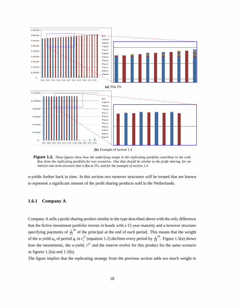
. Figure 1.5(a) shows

how the investments, the u-yield,r f i and the reserve evolve for this product for the same scenario

as figures 1.2(a) and 1.2(b).

The figure implies that the replicating strategy from the previous section adds too much weight to

18

the investment layers further away. A replicating strategyin line with the last section requires the

use of swaptions of which the underlying swap notionals decline by 115

thevery period. Although

it might be possible to find an analytical valuation of this, it is not within the scope of this thesis.

Another way of modeling this would be to use fifteen swaptionsfor every investment layer: one

on a 15 year swap with115 of the investment layer as notional, one on a 14 year swap with2

15 of

the investment layer as notional, etc. Because this is a bit cumbersome and again not in line with

the purpose of this thesis a solution could be to work with underlying swap maturities equal to the

weighted average maturityMq of an investment layer, the use of an average notional that results

in swaptions paying too little in beginning periods, too much during the last periods but are good

on average, or a combination of the two. The trick is then to replace the fifteen swaptions that are

optimally required by significantly less. The trade off in selecting the optimal replicating strategy

will be in the extent to which theM year swap rate is still a good proxy for the u-rate and the

similarity of the swaption payoffs to the profit sharing thatis determined by the turnover structure,

both in time and in size.

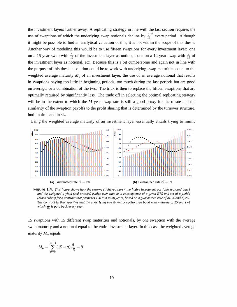
Using the weighted average maturity of an investment layer essentially entails trying to mimic

(a) Guaranteed raterg = 1% (b) Guaranteed raterg = 3%

Figure 1.4. This figure shows how the reserve (light red bars), the fictiveinvestment portfolio (colored bars)and the weighted u-yield (red crosses) evolve over time as a consequence of a given RTS and set of u-yields(black cubes) for a contract that promises 100 mln in 30 years, based on a guaranteed rate of a)1% and b)3%.The contract further specifies that the underlying investment portfolio used bond with maturity of 15 years ofwhich 1

15 is paid back every year.

15 swaptions with 15 different swap maturities and notionals, by one swaption with the average

swap maturity and a notional equal to the entire investment layer. In this case the weighted average

maturityMw equals

Mw =15−1

∑q=0

(15−q)q15

= 8

19

The expiration dates of the swaptions still coincide with the investments layers as before.

Theoretically this would then cause cash flows that will be too large from the second year until

the 8th year and cash flows that will be too low (0) from the 9th until the 15th year.

A strategy that would create cash flows over the entire periodof the 15 years in which the investment

layer influences the profit sharing, but still uses only one swaption per layer, could be the use of an

average notional in 15 year swaptions. The average investment over the 15 years for investmentIi is

Ni =115

15−1

∑q=0

(1− q15

)Igi = 0.533Ig

i .

The superscript inIgi here means that these are again the investments based on the guaranteed rate,

as explained in the last section and, more elaborately, in appendix A.1.1.2.

This strategy would theoretically cause cash flows being toolow during the first years, exactly right

in the middle and to large during the last years.

A disadvantage that is also encountered using a weighted maturity, is that the 8 year and the 15 year

swap rates might not match the u-yield very closely anymore.To adjust for the mismatch between

the u-yield and the 8 and 15 year swap rate an adjustment can however be made to the strike of the

swaptions that should be quite reliable. This would amount in adjustments of respectively 10 basis

points(0.10%) and 50 basis point (0.5%) upwards, followingthe average difference from historical

time series over the last 12 years.

Besides a motivation to use 8 year swaptions is that the 8 yearswap rate can be expected to match

the u-rate more closely then the 15 year swap rate, and that the notional might result in cash flows

more close to the profit sharing during the first 8 years compared to the use of an average notional,

the disadvantage remains that the cash flows following the underlying swaps will not coincide with

the weight of the investment layers. This is because the underlying swaps last 8 years and the layers

15 years. Another question that remains is whether the notionals of the 8 year swaptions should b

based on the 15 year investment policy, in line with the fictive investment portfolio, or on an 8 year

investment policy.

The use of 15 year swaptions with an average notional will circumvent the problem of not taking

into account layers which do influence the profit sharing but might result in differences in cash flows

that are too large. This will be both due to the use of an average notional and due to the fact that 15

year swaptions will cause 15 cash flows, when the swap rate is higher than the strike, whereas profit

sharing causes a maximum of one cash flow, based on the weighted rates over the last 15 years in

r f i .

20

To prevent too much divergence in the cash flow pattern a hybrid of the two, that tries to capture the

fifteen swaptions ideally required for an investment layer in two swaptions, will also be considered.

One hybrid will be based on two swaptions that both have a maturity of 7 years to minimize the

difference between the swap rate and the u-yield. One will have a notional of the average investment

during the first 7 years with a start date equal to the start of the period of the investment, and one

with a notional equal to the average remaining investment during the subsequent 7 years. Note that

this strategy will cause at most fourteen cash flows, seven based on the swap rate in the period the

investment is done, seven based on the swap rate 7 years later. This strategy will cause a u-rate in

periodi to have an influence based on the investments in periodi and investments of 7 periods ago.

This way it will ensure a less diverge cash flow pattern while on average the whole notional of every

layer is still considered, but giving up some of the right weighing because a u-rate in yeari is only

partially weighted by an investment of yeari.

Another approach would be to try mimicking the weighing moreprecise. This would mean that

the swap rates match the u-rate less and it causes more diverge cash flows. A way to do this with

two swaptions would be to use one swaption with a maturity of 15 years and a notional equal to the

average amount of the investment that lasts more than 7 years, and one swaption with a maturity

of 7 years and a notional equal to the average amount of the investment the first 7 years minus the

portion covered by the 15 year swap. Both starting when the investment is made. If the swap rate

in period i would then be higher then the strike this would cause two cashflows during the first 7

years and one cash flow during the last 8. In summary there are then 5 replicating strategies that try

to mimic the profit sharing by a maximum of 2 swaptions per investment layer:

1. Use of one swaption per investment layer using a weighted average swap maturity of 8 years,

notionals based on the investment policy of the fictive portfolio and a strike ofrg+δ +10bps.

2. Use of one swaption per investment layer with a weighted average swap maturity of 8 years,

notionals based on a investment policy following a turnoverstructure specifying notionals are

paid back in full after 8 years and a strike ofrg+δ +10bps.

3. Use of one swaption per investment layer with a swap maturity of 15 years, a weighted

average notional based on the investment policy of the fictive portfolio and a strike of

rg+δ +50bps.

4. Use of two swaptions per investment layer with a swap maturity of 7 years, one with a

weighted notional based on the first 7 years, the other one with maturity of 7 years and a

weighted notional based on the subsequent 7 years. Both following the investment policy of

the fictive portfolio and a strike ofrg+δ .

5. Use of two swaptions per investment layer, one with a swap maturity of 15 years, a weighted

notional based on investments lasting over 7 years (30%Iq) of the notional and a strike of

21

rg + δ + 50bps, the other one with maturity of 7 years, a notional that sets the combined

notional of the two swaptions to the weighted average layer over the first 7 years ((80% -

30%)Iq = 50%Iq) and a strike ofrg + δ . Both following the investment policy of the fictive

portfolio.

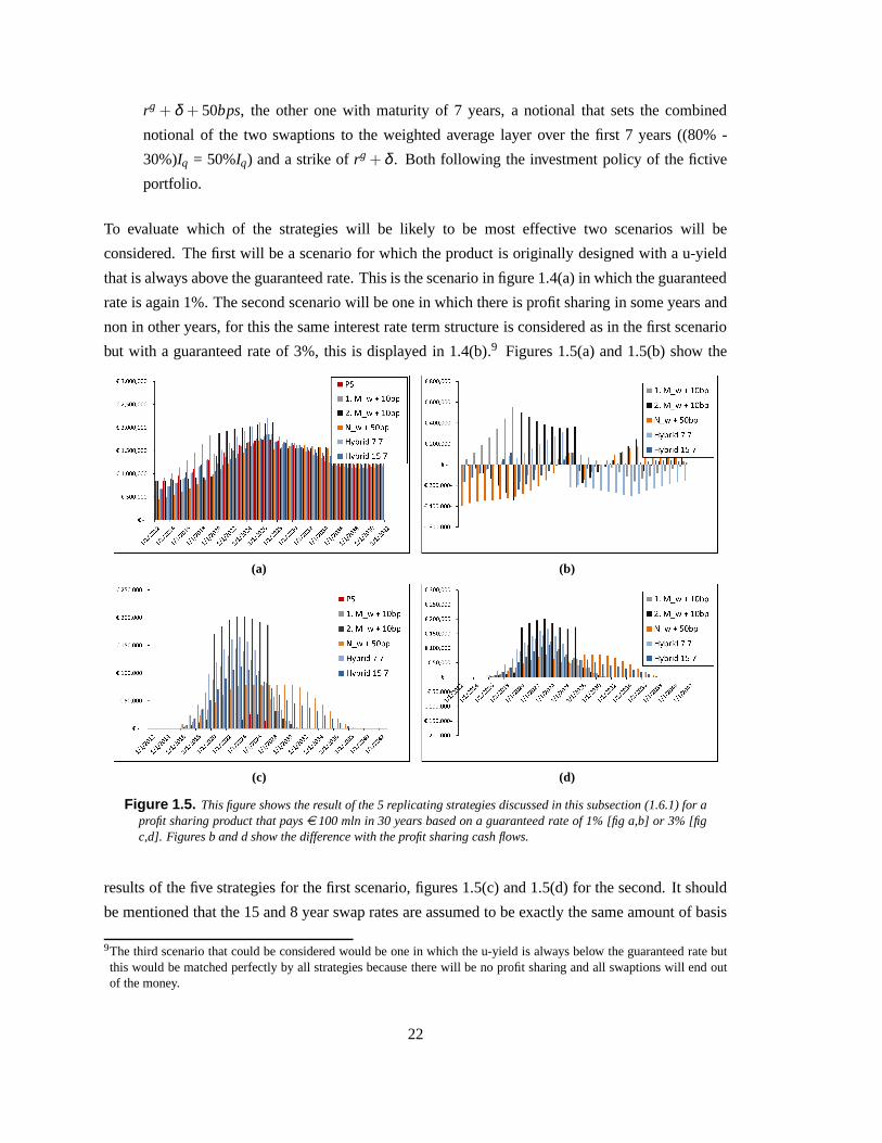
To evaluate which of the strategies will be likely to be most effective two scenarios will be

considered. The first will be a scenario for which the productis originally designed with a u-yield

that is always above the guaranteed rate. This is the scenario in figure 1.4(a) in which the guaranteed

rate is again 1%. The second scenario will be one in which there is profit sharing in some years and

non in other years, for this the same interest rate term structure is considered as in the first scenario

but with a guaranteed rate of 3%, this is displayed in 1.4(b).9 Figures 1.5(a) and 1.5(b) show the

(a) (b)

(c) (d)

Figure 1.5. This figure shows the result of the 5 replicating strategies discussed in this subsection (1.6.1) for aprofit sharing product that payse 100 mln in 30 years based on a guaranteed rate of 1% [fig a,b] or 3% [figc,d]. Figures b and d show the difference with the profit sharing cash flows.

results of the five strategies for the first scenario, figures 1.5(c) and 1.5(d) for the second. It should

be mentioned that the 15 and 8 year swap rates are assumed to beexactly the same amount of basis

9The third scenario that could be considered would be one in which the u-yield is always below the guaranteed rate butthis would be matched perfectly by all strategies because there will be no profit sharing and all swaptions will end outof the money.

22

points above the 7 year swap rate as the upward adjustment of the strikes and the the 7 year swap

rate is a good proxy for the u-rate. This means that the focus here is purely on the replication of

the cash flows from profit sharing by use of a few swaptions whenthe underlying decreases by a

fixed turnover pattern. From this figure it is clear that most strategies are not really satisfactory

during the first years. The first two strategies make use of oneswaption for every layer based on

a weighted average maturity of 8 years but converge more to the profit sharing in later years. The

main advantage of this strategy is that the cash flow pattern will match more closely to the amount

of profit sharings than the strategies that use 15 year swaptions. Also the cash flows match the profit

sharing better in the first years because no average notionalis used. This result is most pronounced

in figure 1.6(a), comparing the orange bar (strategy 3) with the black or grey bar (strategies 1 and

2). However, after a couple of years it is clear that cash flowsstart to diverge significantly compared

to the profit sharing in scenario 1 and exceed the profit sharings by far in scenario 2. Comparing the

two with each other suggest it is important to base the swaption notionals on the re-investments done

in the fictive portfolio and not based on a simplified turnoverstructure that matches the maturity of

the swaptions. The black bar, representing strategy 2, doesnot move as gradual as one would like,

though some smoothing seems to occur at the end.

The third strategy, that uses an averaged notional and 15 year swaptions, results in significantly less

then the profit sharing in the first years of scenario 1 and shows a very diverge cash flow pattern of

twenty three swap payoffs compared to four profit sharing in scenario 2, where they are also at least

twice as large as the profit sharing.

The use of a hybrid strategy seems a good compromise. The use of two 7 year swaptions is attractive

because it is simpler and the 7 year swap rate proxies the u-rate best, a worrying observation is

however that the differences with the profit sharings start to become more significant in periods

further in the future, whereas the other strategies show a greater amount of convergence there.

Though the use of lower maturities results in a number of cashflows from the replicating strategies

that is more close to the number of profit sharings in times like scenario 2, this advantage is offset

by the the extent in which the cash flows are larger than the profit sharings. This strategy also seems

to be expensive, probably due to the use of swaptions having alonger time to expiration, increasing

the time value in the options.

The second hybrid strategy seems to be a good remedy for the disadvantages of the third strategy

that were just pointed out. Also the disadvantage of non-convergence of the first hybrid model does

not occur, this suggests that the last strategy might be the best way to model the replicating portfolio

by just two swaptions per layer.

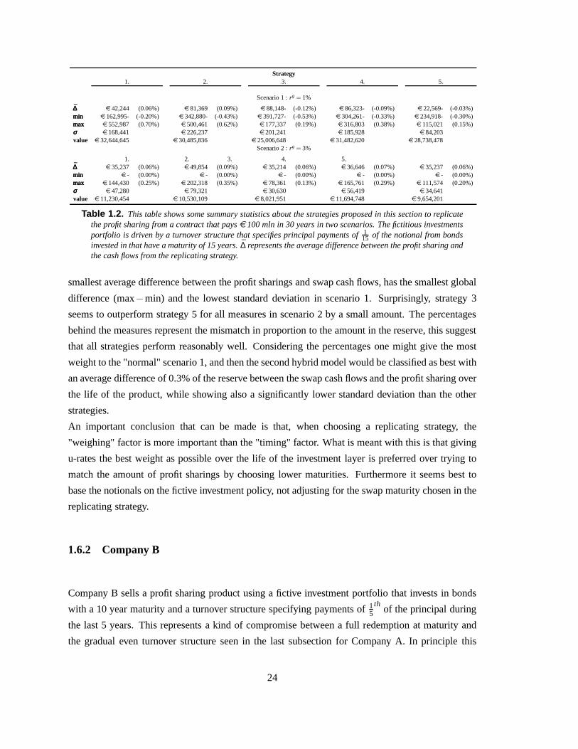
Table 1.2 gives some summary statistics of all replicating strategies. The statistics seem to confirm

with the results from the above analysis as the second hybridstrategy (strategy 5) shows the

23

Strategy1. 2. 3. 4. 5.

Scenario 1 :rg = 1%

∆̄̄∆̄∆ e 42,244 (0.06%) e 81,369 (0.09%) e 88,148- (-0.12%) e 86,323- (-0.09%) e 22,569- (-0.03%)minminmin e 162,995- (-0.20%) e 342,880- (-0.43%) e 391,727- (-0.53%) e 304,261- (-0.33%) e 234,918- (-0.30%)maxmaxmax e 552,987 (0.70%) e 500,461 (0.62%) e 177,337 (0.19%) e 316,803 (0.38%) e 115,021 (0.15%)σσσ e 168,441 e 226,237 e 201,241 e 185,928 e 84,203value e 32,644,645 e 30,485,836 e 25,006,648 e 31,482,620 e 28,738,478

Scenario 2 :rg = 3%

1. 2. 3. 4. 5.∆̄̄∆̄∆ e 35,237 (0.06%) e 49,854 (0.09%) e 35,214 (0.06%) e 36,646 (0.07%) e 35,237 (0.06%)minminmin e - (0.00%) e - (0.00%) e - (0.00%) e - (0.00%) e - (0.00%)maxmaxmax e 144,430 (0.25%) e 202,318 (0.35%) e 78,361 (0.13%) e 165,761 (0.29%) e 111,574 (0.20%)σσσ e 47,280 e 79,321 e 30,630 e 56,419 e 34,641value e 11,230,454 e 10,530,109 e 8,021,951 e 11,694,748 e 9,654,201

Table 1.2. This table shows some summary statistics about the strategies proposed in this section to replicatethe profit sharing from a contract that payse 100 mln in 30 years in two scenarios. The fictitious investmentsportfolio is driven by a turnover structure that specifies principal payments of115 of the notional from bondsinvested in that have a maturity of 15 years.∆̄ represents the average difference between the profit sharing andthe cash flows from the replicating strategy.

smallest average difference between the profit sharings andswap cash flows, has the smallest global

difference (max−min) and the lowest standard deviation in scenario 1. Surprisingly, strategy 3

seems to outperform strategy 5 for all measures in scenario 2by a small amount. The percentages

behind the measures represent the mismatch in proportion tothe amount in the reserve, this suggest

that all strategies perform reasonably well. Considering the percentages one might give the most

weight to the "normal" scenario 1, and then the second hybridmodel would be classified as best with

an average difference of 0.3% of the reserve between the swapcash flows and the profit sharing over

the life of the product, while showing also a significantly lower standard deviation than the other

strategies.

An important conclusion that can be made is that, when choosing a replicating strategy, the

"weighing" factor is more important than the "timing" factor. What is meant with this is that giving

u-rates the best weight as possible over the life of the investment layer is preferred over trying to

match the amount of profit sharings by choosing lower maturities. Furthermore it seems best to

base the notionals on the fictive investment policy, not adjusting for the swap maturity chosen in the

replicating strategy.

1.6.2 Company B

Company B sells a profit sharing product using a fictive investment portfolio that invests in bonds

with a 10 year maturity and a turnover structure specifying payments of15th

of the principal during

the last 5 years. This represents a kind of compromise between a full redemption at maturity and

the gradual even turnover structure seen in the last subsection for Company A. In principle this

24

could be replicated by 5 swaptions for every period: a 10 yearswaption with a notional of15th

of the

investment layer, a 9 year swaption with a notional of25

ththe investment layer, etc., and ending with

a 5 year swaption having a notional equal to the entire amountof the investment layer. Here this

portfolio will be replicated using again a maximum of two swaptions. It can be expected that the

use of a weighted average maturity will result in better results than in the last subsection because

repayments of an investment layer begin only after 5 years and last only 5 years. Results from the

last section however suggest that the weighing should be replicated as good as possible. This would

result in using a hybrid strategy consisting of 1 swaption with a notional equal to the 40% of the

investment and a maturity of 5 years and 1 with a maturity of 10years and a notional equal to the

average investment layer during the last 5 years (60%). The strategy that rivaled the hybrid one in

the last section, using a weighted average notional over thefull maturity, will also be considered.

In summary the following strategies will be considered:

1. Use of one swaption per investment layer with a weighted average swap maturity of

Mw =15

(

10+9+8+7+6)

= 8,

a notional equal to the full amount of the investment layer and a strike ofrg+δ +10bps.

2. Use of one swaption per investment layer using a notional based on the weighted average

investment of

Ni =110

MwIgi = 0.8Ig

i ,

a swap maturity equal to the maturity of the investments of the fictive portfolio and a strike of

rg+δ +20bps.

3. Use of two swaptions per investment layer, one with maturity of 10 years, a weighted notional

based on investments lasting over 5 years (60% of the layer) and a strike ofrg+ δ +20bps,

the other one with maturity of 5 years, a notional equal to 40%of the full amount of the

investment layer of the period and a strike ofrg+δ −15bps.

All notionals are based on the investment policy of the fictive portfolio.

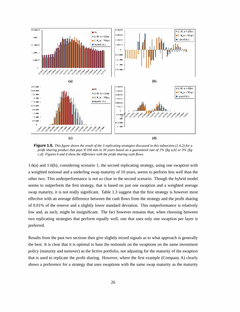
The figures below give the results for these replicating strategies in the same way as the last

subsection. Again two scenarios are considered, one where all u-rates during the life of the contract

are above the guaranteed rate of 1%, causing profit sharings every year, and one scenario where there

is profit sharing in some years and none in others due to a higher guaranteed rate of 3%. From figures

25

(a) (b)

(c) (d)

Figure 1.6. This figure shows the result of the 3 replicating strategies discussed in this subsection (1.6.2) for aprofit sharing product that payse 100 mln in 30 years based on a guaranteed rate of 1% [fig a,b] or 3% [figc,d]. Figures b and d show the difference with the profit sharing cash flows.

1.6(a) and 1.6(b), considering scenario 1, the second replicating strategy, using one swaption with

a weighted notional and a underling swap maturity of 10 years, seems to perform less well than the

other two. This underperformance is not so clear in the second scenario. Though the hybrid model

seems to outperform the first strategy, that is based on just one swaption and a weighted average

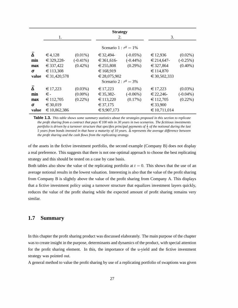
swap maturity, it is not really significant. Table 1.3 suggest that the first strategy is however most

effective with an average difference between the cash flows from the strategy and the profit sharing

of 0.01% of the reserve and a slightly lower standard deviation. This outperformance is relatively

low and, as such, might be insignificant. The fact however remains that, when choosing between

two replicating strategies that perform equally well, one that uses only one swaption per layer is

preferred.

Results from the past two sections then give slightly mixed signals as to what approach is generally

the best. It is clear that it is optimal to base the notionals on the swaptions on the same investment

policy (maturity and turnover) as the fictive portfolio, notadjusting for the maturity of the swaption

that is used to replicate the profit sharing. However, where the first example (Company A) clearly

shows a preference for a strategy that uses swaptions with the same swap maturity as the maturity

26

Strategy1. 2. 3.

Scenario 1 :rg = 1%

∆̄̄∆̄∆ e 4,128 (0.01%) e 32,494- (-0.05%) e 12,936 (0.02%)minminmin e 329,228- (-0.41%) e 361,616- (-0.44%) e 214,647- (-0.25%)maxmaxmax e 337,422 (0.42%) e 255,808 (0.29%) e 327,864 (0.40%)σσσ e 113,308 e 168,919 e 114,870value e 31,420,578 e 28,075,902 e 30,502,333

Scenario 2 :rg = 3%

∆̄̄∆̄∆ e 17,223 (0.03%) e 17,223 (0.03%) e 17,223 (0.03%)minminmin e - (0.00%) e 35,382- (-0.06%) e 22,246- (-0.04%)maxmaxmax e 112,705 (0.22%) e 113,220 (0.17%) e 112,705 (0.22%)σσσ e 30,019 e 37,175 e 33,900value e 10,862,386 e 9,907,173 e 10,711,014

Table 1.3. This table shows some summary statistics about the strategies proposed in this section to replicatethe profit sharing from a contract that payse 100 mln in 30 years in two scenarios. The fictitious investmentsportfolio is driven by a turnover structure that specifies principal payments of15 of the notional during the last5 years from bonds invested in that have a maturity of 10 years. ∆̄ represents the average difference betweenthe profit sharing and the cash flows from the replicating strategy.

of the assets in the fictive investment portfolio, the secondexample (Company B) does not display

a real preference. This suggests that there is not one optimal approach to choose the best replicating

strategy and this should be tested on a case by case basis.

Both tables also show the value of the replicating portfolioat t = 0. This shows that the use of an

average notional results in the lowest valuation. Interesting is also that the value of the profit sharing

from Company B is slightly above the value of the profit sharing from Company A. This displays

that a fictive investment policy using a turnover structure that equalizes investment layers quickly,

reduces the value of the profit sharing while the expected amount of profit sharing remains very

similar.

1.7 Summary

In this chapter the profit sharing product was discussed elaborately. The main purpose of the chapter

was to create insight in the purpose, determinants and dynamics of the product, with special attention

for the profit sharing element. In this, the importance of theu-yield and the fictive investment

strategy was pointed out.

A general method to value the profit sharing by use of a replicating portfolio of swaptions was given

27

and the performance of this valuation was evaluated for several scenarios. Results showed that

the method produces robust results for a basic profit sharingproduct. For products specified by a

more complicated investment strategy, a replicating portfolio could in theory still produce accurate

results. Because this does however not have any practical value, here strategies to replicate the

products by use of a simple portfolio were constructed. In doing this one has to find the optimal

trade off between trying to replicate the number of profit sharings and trying to replicate the right

weight that investments have. What this trade off should be depends specifically on the turnover

structure of the fictitious investments and has to be determined on a case by case basis.

28

Chapter 2

Risks

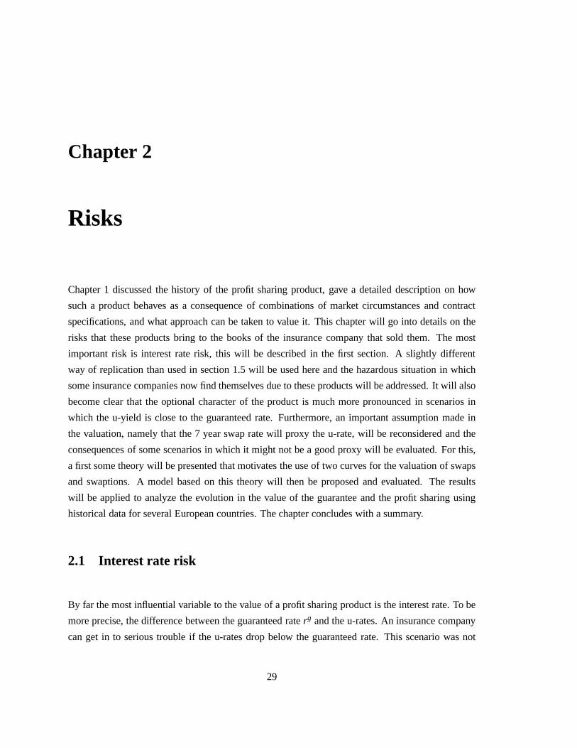
Chapter 1 discussed the history of the profit sharing product, gave a detailed description on how

such a product behaves as a consequence of combinations of market circumstances and contract

specifications, and what approach can be taken to value it. This chapter will go into details on the

risks that these products bring to the books of the insurancecompany that sold them. The most

important risk is interest rate risk, this will be describedin the first section. A slightly different

way of replication than used in section 1.5 will be used here and the hazardous situation in which

some insurance companies now find themselves due to these products will be addressed. It will also

become clear that the optional character of the product is much more pronounced in scenarios in

which the u-yield is close to the guaranteed rate. Furthermore, an important assumption made in

the valuation, namely that the 7 year swap rate will proxy theu-rate, will be reconsidered and the

consequences of some scenarios in which it might not be a goodproxy will be evaluated. For this,

a first some theory will be presented that motivates the use oftwo curves for the valuation of swaps

and swaptions. A model based on this theory will then be proposed and evaluated. The results

will be applied to analyze the evolution in the value of the guarantee and the profit sharing using

historical data for several European countries. The chapter concludes with a summary.

2.1 Interest rate risk

By far the most influential variable to the value of a profit sharing product is the interest rate. To be

more precise, the difference between the guaranteed raterg and the u-rates. An insurance company

can get in to serious trouble if the u-rates drop below the guaranteed rate. This scenario was not

29

really discussed in chapter 1 because this is not a scenario for which this product was designed.

The insurance company will be obligated to live up to the contractual agreement of paying the

policyholder interest equal torg in this case, while the fictive investment portfolio only generates

r f i , that will be lower thanrg if the u-rates stay low over a large enough time span. For a scenario in

which all u-rates are below the guaranteed rate (ui < rg), the value of the profit sharing will be very

close to zero.1 The swaptions specified in the replicating portfolio from section 1.5 will all end out

of the money and the value of the contract will be equal to a zero coupon bond paying the guaranteed

amount at maturity. Though this valuation is still correct it is not very informative for the interest

rate risk anymore. Another approach to the replication of this product would be to use swaptions

for the downside (r f i < rg), modeling the guarantee explicitly, instead of the upside(r f i > rg), that

models the profit sharing. In this way it will become clear howexpensive these products currently

are for the insurance companies, as interest rates are at an all time low. Essentially exactly the

same scenario repeats itself now as in the late nineties. Back then insurance companies sold the

product with guaranteed rates of around 8%, because interest rates were above 10% and the implicit

guaranteed rates were considered harmless. Most insurancecompanies that experienced the drop

in interest rates to 4-6% just lowered the guaranteed rate for the policies to around 3% and are

therefore likely to face similar difficulties due to this guarantee as before.

In summary two methods to replicate the cash flows from a contract that promises to paye 100 mln

in 30 years based a guaranteed rate of 3% and a fictive investment portfolio that invests in 7 year

u-rate bonds with a turnover structure specifying full principal payments at maturity of the bond,

are:

1. Modeling the profit sharing explicitly with the results ofsection 1.5 and a zero coupon bond.

i) 30 payer swaptions with expiration dates just before the start of every year, an underlying

swap maturity of seven years, a strike equal torg and a notional determined by the the

investment strategy of the fictive portfolio based on the guaranteed rate (see section 1.5

and appendix A.1.1.2).

ii) A zero coupon bond payinge 100 mln in 30 years.

2. Modeling the guarantee explicitly using receiver swaptions and bonds yieldingui .

i) 30 receiver swaptions with expiration dates just before the start of every year, an

underlying swap maturity of seven years, a strike equal torg and a notional determined

by the the investment strategy of the fictive portfolio basedon the guaranteed rate.

ii) Investments in bonds equal to the ones specified by the investment policy of the fictive

portfolio.

1There will be some time value for the optional profit sharing.

30

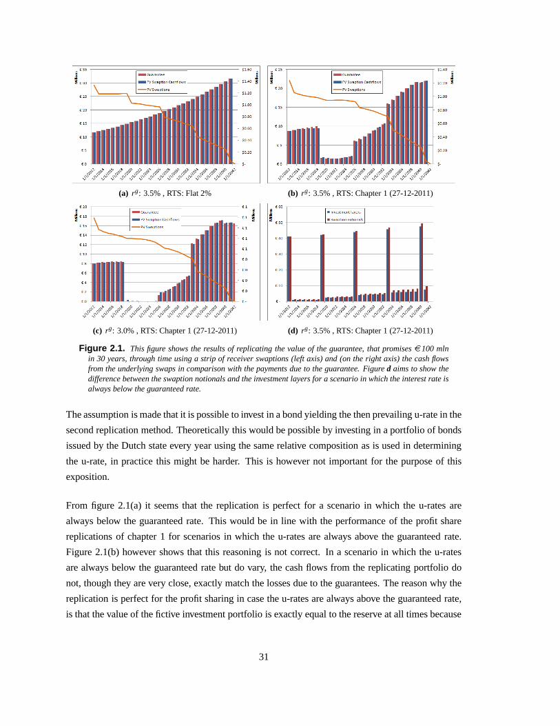
(a) rg: 3.5% , RTS: Flat 2% (b) rg: 3.5% , RTS: Chapter 1 (27-12-2011)

(c) rg: 3.0% , RTS: Chapter 1 (27-12-2011) (d) rg: 3.5% , RTS: Chapter 1 (27-12-2011)

Figure 2.1. This figure shows the results of replicating the value of the guarantee, that promisese 100 mlnin 30 years, through time using a strip of receiver swaptions(left axis) and (on the right axis) the cash flowsfrom the underlying swaps in comparison with the payments due to the guarantee. Figured aims to show thedifference between the swaption notionals and the investment layers for a scenario in which the interest rate isalways below the guaranteed rate.

The assumption is made that it is possible to invest in a bond yielding the then prevailing u-rate in the

second replication method. Theoretically this would be possible by investing in a portfolio of bonds

issued by the Dutch state every year using the same relative composition as is used in determining

the u-rate, in practice this might be harder. This is howevernot important for the purpose of this

exposition.

From figure 2.1(a) it seems that the replication is perfect for a scenario in which the u-rates are

always below the guaranteed rate. This would be in line with the performance of the profit share

replications of chapter 1 for scenarios in which the u-ratesare always above the guaranteed rate.

Figure 2.1(b) however shows that this reasoning is not correct. In a scenario in which the u-rates

are always below the guaranteed rate but do vary, the cash flows from the replicating portfolio do

not, though they are very close, exactly match the losses dueto the guarantees. The reason why the

replication is perfect for the profit sharing in case the u-rates are always above the guaranteed rate,

is that the value of the fictive investment portfolio is exactly equal to the reserve at all times because

31

the profit share is paid out. This has as result that all investment layers in the different u-rates,

of which the coupons set the portfolio return on which the profit sharing is based, will match the

swaption notionals exactly. For the replication of the guarantee this does however not hold because

the fictive investment portfolio will start to diverge from the reserve when the u-rates are below the

guaranteed rate, meaning that the investments layers will in general not be equal to the swaption

notionals. Figure 2.1(d) shows this. The mismatch in all scenarios is however very small, meaning

that this replication method can assign a value to the guarantee in which one can be confident. The

scenario of figure 2.1(c) is probably the most representative with a guaranteed rate of 3%, here the

value of the guarantee is close toe 18 mln and in this scenario all cash flows resulting from the

guarantee eventually amount to overe 13 mln, taking into account profit sharing in 7 periods and

accrued interests. The most important message coming forthfrom this section is then that the value

of this guarantee is very significant and that it can be expected that a lot of insurance companies are

currently facing big losses due to the selling of these embedded options. This is also confirmed by

a paragraph in a recent semiannual financial stability report from the Dutch central bank, see DNB

(2012), in which they explicitly mention "the pressure on capital buffers due to the issuance of high

guarantees in the past...".

2.2 Valuation and Swap-Government spread

All computations in this thesis and in most of the earlier research have been based on the assumption

that the swap rate is a good proxy for the u-rate, or at least the "part" u-yield (see section 1.3). This

assumption makes life a lot easier with respect to valuationand risk management practices, but it

entails a substantial risk. If the u-rate does not proxy the 7year swap rate, this will result in a faulty

valuation or an ineffective hedge. For example, using the replication strategy of the last chapter, the

swaptions pay out if the swap rate is above the guaranteed rate but the profit sharing pays out when

the weighted u-rate is above the guaranteed rate. This meansthat if such a scenario presents itself,

an insurance company will sell products on which it is likelyto make a loss or buys a hedge that is

ineffective.2

What is needed to value this product using the same replicating strategy as in chapter 1, while not

making this assumption, is a way to value swaptions based on two interest rate curves; one as a

reference rate and one for discounting the cash flows. To see why this makes sense and how this

would be done, some swap and swaption theory will be discussed.

2It should be emphasized that this risk is imposed due to the use of the 7 year swap rate as a proxy for the u-rate and notdue to the use of replicating portfolio for valuation.

32

2.2.1 Swaps, Swaprates and Swaptions

A swaption gives the right, but not the obligation, to enter aswap at a predetermined fixed rate. An

interest rate swap represents the exchange of a fixed interest for a floating interest during a specified

period of time on an agreed notional. The value of this (payer) swap is then best defined by the

difference between a floating rate bond and a fixed rate bond:

Vswapt = Bf l −Bf ix = N

n

∑q=1

df t,q

(

r f wt,q − r f ix), (2.1)

with Vt the value of the swap at timet, N the notional,df t,q the discount factor at timet for a cash

flow in periodq andr f wt,q the forward rate in periodq at timet. This formula can be used to compute

the swap raterswapt at time t . The swap rate is the rate that sets the value of this contractequal

to zero using forward rates and zero rates, this is usually done at inception of a swap contract to

computer f ix = rswapt . Later, the floating rates (and swap rate that sets the value of the contract to

zero at a different point in time) will vary from the rates at time t and the swap will take on a value

different from zero. In this case the value will be greater than zero if the expected floating rates are

higher than the fixed rate during the period of the swap.

The same curve is often used in computing the discount factors df t,q and in computing the forward

ratesr f wt,q . The interest rate curve used to compute the discount factors should be a "risk free" curve

as swap contracts allow for several measures that minimize risk of payments not being made. The

forward rates include a small credit risk premium3, mostly representing the creditworthiness of

banks providing Libor4. It is then convenient to use the same curve and add the premium to this for

the computation of the forward rates.

To determine the value of a swaption att only the swap rate is used. Because this rate sets the value

of a similar contract to zero at different points in time, thedifference between the contractual fixed

rate and the swap rate at timet can capture the value. The value of the swaption is then computed

as the discounted difference (if positive) between the expected swap rate at expiration and the fixed

rate that was agreed upon for the amount of interest exchanges n. This expectation is computed in a

risk neutral setting, hence the subscriptQ, in the same way as Black and Scholes (1973) introduced

3It is important to realize that this credit risk premium is different from the premium that the contract holder would payif he issued a bond.

4London interbank offered rate.

33

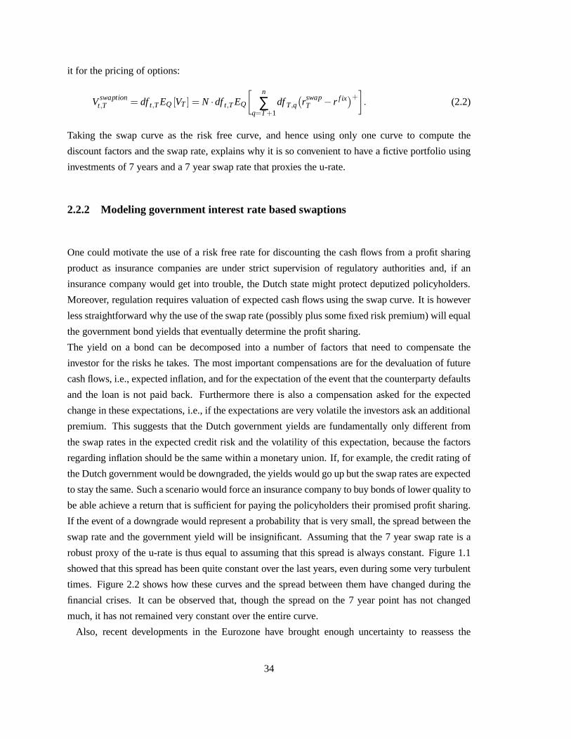
it for the pricing of options:

Vswaptiont,T = df t,TEQ [VT ] = N ·df t,TEQ

[ n

∑q=T+1

dfT,q

(

rswapT − r f ix)+

]

. (2.2)

Taking the swap curve as the risk free curve, and hence using only one curve to compute the

discount factors and the swap rate, explains why it is so convenient to have a fictive portfolio using

investments of 7 years and a 7 year swap rate that proxies the u-rate.

2.2.2 Modeling government interest rate based swaptions

One could motivate the use of a risk free rate for discountingthe cash flows from a profit sharing

product as insurance companies are under strict supervision of regulatory authorities and, if an

insurance company would get into trouble, the Dutch state might protect deputized policyholders.

Moreover, regulation requires valuation of expected cash flows using the swap curve. It is however

less straightforward why the use of the swap rate (possibly plus some fixed risk premium) will equal

the government bond yields that eventually determine the profit sharing.

The yield on a bond can be decomposed into a number of factors that need to compensate the

investor for the risks he takes. The most important compensations are for the devaluation of future

cash flows, i.e., expected inflation, and for the expectationof the event that the counterparty defaults

and the loan is not paid back. Furthermore there is also a compensation asked for the expected

change in these expectations, i.e., if the expectations arevery volatile the investors ask an additional

premium. This suggests that the Dutch government yields arefundamentally only different from

the swap rates in the expected credit risk and the volatilityof this expectation, because the factors

regarding inflation should be the same within a monetary union. If, for example, the credit rating of

the Dutch government would be downgraded, the yields would go up but the swap rates are expected

to stay the same. Such a scenario would force an insurance company to buy bonds of lower quality to

be able achieve a return that is sufficient for paying the policyholders their promised profit sharing.

If the event of a downgrade would represent a probability that is very small, the spread between the

swap rate and the government yield will be insignificant. Assuming that the 7 year swap rate is a

robust proxy of the u-rate is thus equal to assuming that thisspread is always constant. Figure 1.1

showed that this spread has been quite constant over the lastyears, even during some very turbulent

times. Figure 2.2 shows how these curves and the spread between them have changed during the

financial crises. It can be observed that, though the spread on the 7 year point has not changed

much, it has not remained very constant over the entire curve.

Also, recent developments in the Eurozone have brought enough uncertainty to reassess the

34

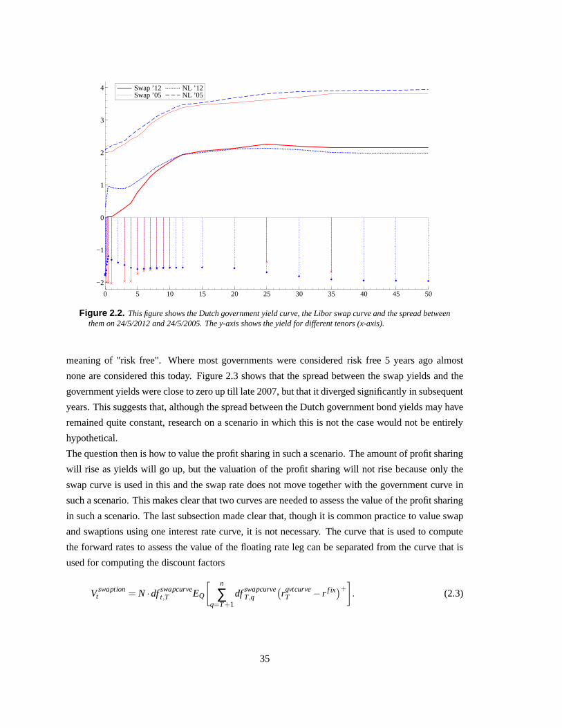
Swap ’12 Swap ’05

NL ’12 NL ’05

0 5 10 15 20 25 30 35 40 45 50

−2

−1

0

1

2

3

4 Swap ’12 Swap ’05

NL ’12 NL ’05

Figure 2.2. This figure shows the Dutch government yield curve, the Liborswap curve and the spread betweenthem on 24/5/2012 and 24/5/2005. The y-axis shows the yield for different tenors (x-axis).

meaning of "risk free". Where most governments were considered risk free 5 years ago almost

none are considered this today. Figure 2.3 shows that the spread between the swap yields and the

government yields were close to zero up till late 2007, but that it diverged significantly in subsequent

years. This suggests that, although the spread between the Dutch government bond yields may have

remained quite constant, research on a scenario in which this is not the case would not be entirely

hypothetical.

The question then is how to value the profit sharing in such a scenario. The amount of profit sharing

will rise as yields will go up, but the valuation of the profit sharing will not rise because only the

swap curve is used in this and the swap rate does not move together with the government curve in

such a scenario. This makes clear that two curves are needed to assess the value of the profit sharing

in such a scenario. The last subsection made clear that, though it is common practice to value swap

and swaptions using one interest rate curve, it is not necessary. The curve that is used to compute

the forward rates to assess the value of the floating rate leg can be separated from the curve that is

used for computing the discount factors

Vswaptiont = N ·dfswapcurve

t,T EQ

[ n

∑q=T+1

dfswapcurveT,q

(

rgvtcurveT − r f ix)+

]

. (2.3)

35

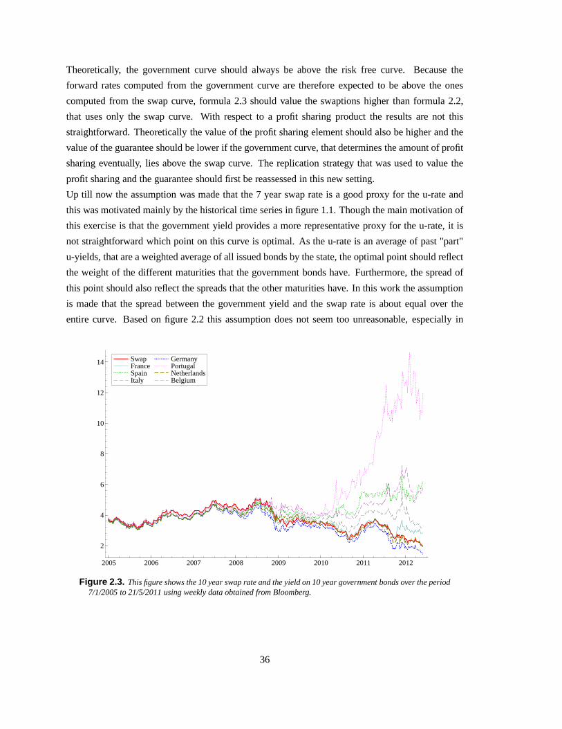
Theoretically, the government curve should always be abovethe risk free curve. Because the

forward rates computed from the government curve are therefore expected to be above the ones

computed from the swap curve, formula 2.3 should value the swaptions higher than formula 2.2,

that uses only the swap curve. With respect to a profit sharingproduct the results are not this

straightforward. Theoretically the value of the profit sharing element should also be higher and the

value of the guarantee should be lower if the government curve, that determines the amount of profit

sharing eventually, lies above the swap curve. The replication strategy that was used to value the

profit sharing and the guarantee should first be reassessed inthis new setting.

Up till now the assumption was made that the 7 year swap rate isa good proxy for the u-rate and

this was motivated mainly by the historical time series in figure 1.1. Though the main motivation of

this exercise is that the government yield provides a more representative proxy for the u-rate, it is

not straightforward which point on this curve is optimal. Asthe u-rate is an average of past "part"

u-yields, that are a weighted average of all issued bonds by the state, the optimal point should reflect

the weight of the different maturities that the government bonds have. Furthermore, the spread of

this point should also reflect the spreads that the other maturities have. In this work the assumption

is made that the spread between the government yield and the swap rate is about equal over the

entire curve. Based on figure 2.2 this assumption does not seem too unreasonable, especially in

Swap France Spain Italy

Germany Portugal Netherlands Belgium

2005 2006 2007 2008 2009 2010 2011 2012

2

4

6

8

10

12

14 Swap France Spain Italy

Germany Portugal Netherlands Belgium

Figure 2.3. This figure shows the 10 year swap rate and the yield on 10 year government bonds over the period7/1/2005 to 21/5/2011 using weekly data obtained from Bloomberg.

36

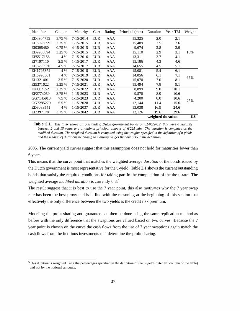
Identifier Coupon Maturity Curr Rating Principal (mln) Duration YearsTM Weight

ED3904759 3.75 % 7-15-2014 EUR AAA 15,325 2.0 2.1

10%

EH8926899 2.75 % 1-15-2015 EUR AAA 15,489 2.5 2.6EI9395480 0.75 % 4-15-2015 EUR AAA 9,674 2.8 2.9ED9903094 3.25 % 7-15-2015 EUR AAA 15,110 2.9 3.1EF5517158 4 % 7-15-2016 EUR AAA 13,311 3.7 4.1EI7197110 2.5 % 1-15-2017 EUR AAA 15,186 4.3 4.6EG6293930 4.5 % 7-15-2017 EUR AAA 14,655 4.5 5.1EH1795374 4 % 7-15-2018 EUR AAA 15,081 5.4 6.1

65%EH6998361 4 % 7-15-2019 EUR AAA 14,056 6.1 7.1EI1321401 3.5 % 7-15-2020 EUR AAA 15,070 7.0 8.1EI5371022 3.25 % 7-15-2021 EUR AAA 15,494 7.8 9.1EJ0062152 2.25 % 7-15-2022 EUR AAA 8,899 9.0 10.1

25%

EF2774059 3.75 % 1-15-2023 EUR AAA 9,870 8.9 10.6GG7145913 7.5 % 1-15-2023 EUR AAA 4,200 8.0 10.6GG7295270 5.5 % 1-15-2028 EUR AAA 12,144 11.4 15.6ED9083541 4 % 1-15-2037 EUR AAA 13,038 16.9 24.6EI2397178 3.75 % 1-15-2042 EUR AAA 12,126 19.6 29.6

weighted duration 6.8

Table 2.1. This table shows all outstanding Dutch government bonds on 31/05/2012, that have a maturitybetween 2 and 15 years and a minimal principal amount ofe 225 mln. The duration is computed as themodified duration. The weighted duration is computed using the weights specified in the definition of u-yieldsand the median of durations belonging to maturity ranges that are also in the definition

2005. The current yield curves suggest that this assumptiondoes not hold for maturities lower than

6 years.

This means that the curve point that matches the weighted averagedurationof the bonds issued by

the Dutch government is most representative for the u-yield. Table 2.1 shows the current outstanding

bonds that satisfy the required conditions for taking part in the computation of the the u-rate. The

weighted averagemodified durationis currently 6.8.5

The result suggest that it is best to use the 7 year point, thisalso motivates why the 7 year swap

rate has been the best proxy and is in line with the reasoning at the beginning of this section that

effectively the only difference between the two yields is the credit risk premium.

Modeling the profit sharing and guarantee can then be done using the same replication method as

before with the only difference that the swaptions are valued based on two curves. Because the 7

year point is chosen on the curve the cash flows from the use of 7year swaptions again match the

cash flows from the fictitious investments that determine theprofit sharing.

5This duration is weighted using the percentages specified inthe definition of the u-yield (outer left column of the table)and not by the notional amounts.

37

2.2.3 Model evaluation

To evaluate the performance of the model, results from the new replication method will be analyzed

for both the profit sharing element and the guarantee. In bothcases the value is computed for

scenarios of varying government spreads and guaranteed rates. By using two curves in the valuation,

the value of the portfolio of swaptions is also sensitive to changes in these two curves. The value

and the sensitivity, measured as the change in value of the swaption portfolio as a consequence of a

parallel shift upwards of 1 basis point in the curve, is displayed in tables 2.2 and 2.3 (respectively

the profit sharing and the guarantee). The percentages to theright of all values computed using the

new model represent the percentual change in value relativeto the original (old) model. Because

the original model is only sensitive towards one curve, these changes concerning the sensitivities

are not entirely comparable. Therefore the difference between the sum of the sensitivities in the

new model and the one of the old model is also computed and expressed as percentage fourthly in

all scenarios. Summing these values can be motivated by the fact that a change in the swap curve

is often followed by the same change in government curves. This is also in line with the reasoning

that the government curve from a Eurozone member country is equal to a risk free curve plus some

credit spread.

NB.

It should be emphasized that in the computation of the value of all swaptions, so also those based on

government curves, only the volatilities of the swap curvesare used. These are implied volatilities extracted

from swaption quotes in the market and, as there are no government interest rate based options traded, are

not available for government rates. The reader should be aware that this can however have a significant

effect on the value of the profit sharing and guarantee. Although volatilities can be expected to rise when

spreads increase and this effect is not expected to be negligible, in this paper only the direct effect of the swap

government spread is evaluated.

The model seems to value the profit sharing correctly. If the spread between the swap curve and

the government curve is zero, the value is exactly similar for the two models. Also the sum of the

two sensitivities equals the one from the original model. Ifthe spread is exactly one basis point, the

value change by the amount that is displayed for the sensitivity towards the forward curve (∆ f w).

Furthermore, the direction of the value is as expected, because it increases when the spread increases

and decreases when the guaranteed rate decreases. One can also observe that the sensitivity towards

the swap curve is always negative and the sensitivity is always positive towards the forward curve.

This is a logical consequence of the fact that the present value of all swaptions decrease when the

discount rate increases and the "in the moneyness" of these options increase when spreads increase.

38

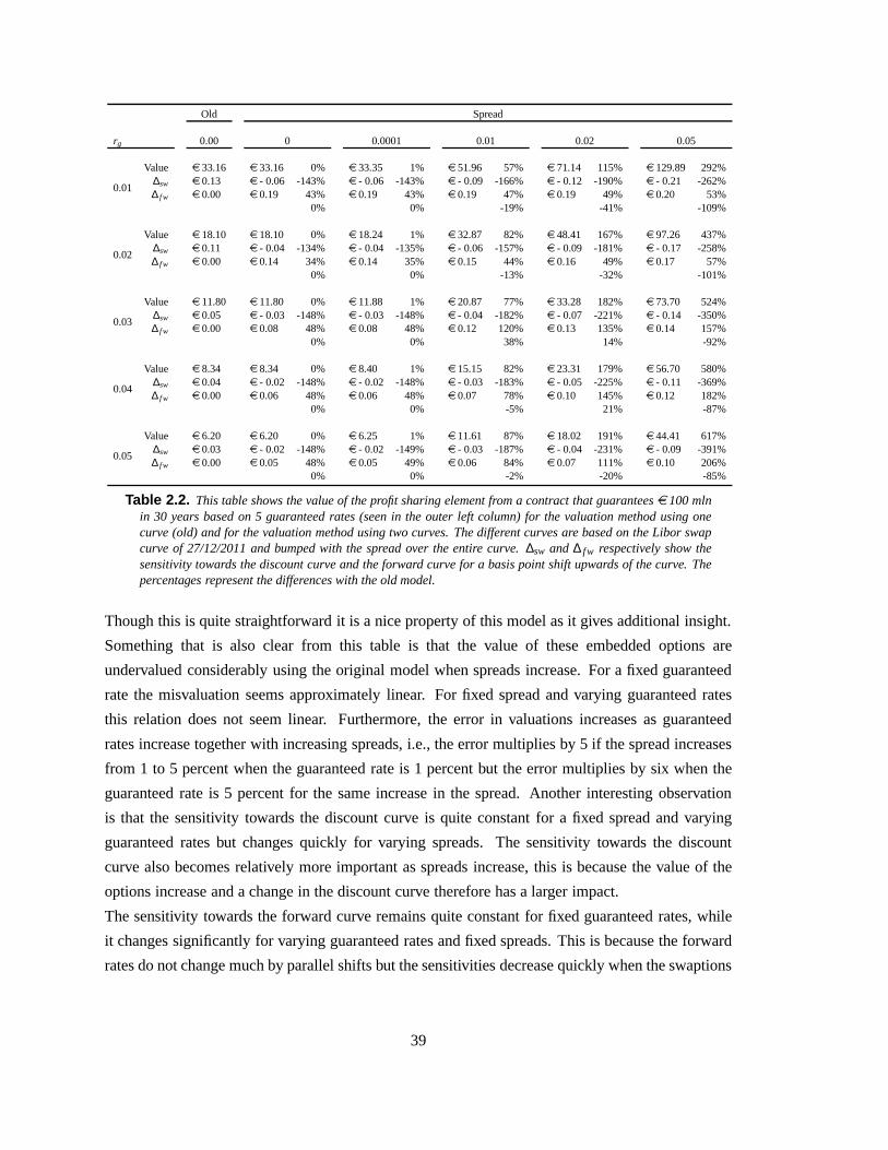
Old Spread

rg 0.00 0 0.0001 0.01 0.02 0.05

0.01

Value e 33.16 e 33.16 0% e 33.35 1% e 51.96 57% e 71.14 115% e 129.89 292%∆sw e 0.13 e - 0.06 -143% e - 0.06 -143% e - 0.09 -166% e - 0.12 -190% e - 0.21 -262%∆ f w e 0.00 e 0.19 43% e 0.19 43% e 0.19 47% e 0.19 49% e 0.20 53%

0% 0% -19% -41% -109%

0.02

Value e 18.10 e 18.10 0% e 18.24 1% e 32.87 82% e 48.41 167% e 97.26 437%∆sw e 0.11 e - 0.04 -134% e - 0.04 -135% e - 0.06 -157% e - 0.09 -181% e - 0.17 -258%∆ f w e 0.00 e 0.14 34% e 0.14 35% e 0.15 44% e 0.16 49% e 0.17 57%

0% 0% -13% -32% -101%

0.03

Value e 11.80 e 11.80 0% e 11.88 1% e 20.87 77% e 33.28 182% e 73.70 524%∆sw e 0.05 e - 0.03 -148% e - 0.03 -148% e - 0.04 -182% e - 0.07 -221% e - 0.14 -350%∆ f w e 0.00 e 0.08 48% e 0.08 48% e 0.12 120% e 0.13 135% e 0.14 157%

0% 0% 38% 14% -92%

0.04

Value e 8.34 e 8.34 0% e 8.40 1% e 15.15 82% e 23.31 179% e 56.70 580%∆sw e 0.04 e - 0.02 -148% e - 0.02 -148% e - 0.03 -183% e - 0.05 -225% e - 0.11 -369%∆ f w e 0.00 e 0.06 48% e 0.06 48% e 0.07 78% e 0.10 145% e 0.12 182%

0% 0% -5% 21% -87%

0.05

Value e 6.20 e 6.20 0% e 6.25 1% e 11.61 87% e 18.02 191% e 44.41 617%∆sw e 0.03 e - 0.02 -148% e - 0.02 -149% e - 0.03 -187% e - 0.04 -231% e - 0.09 -391%∆ f w e 0.00 e 0.05 48% e 0.05 49% e 0.06 84% e 0.07 111% e 0.10 206%

0% 0% -2% -20% -85%

Table 2.2. This table shows the value of the profit sharing element from acontract that guaranteese 100 mlnin 30 years based on 5 guaranteed rates (seen in the outer leftcolumn) for the valuation method using onecurve (old) and for the valuation method using two curves. The different curves are based on the Libor swapcurve of 27/12/2011 and bumped with the spread over the entire curve. ∆sw and ∆ fw respectively show thesensitivity towards the discount curve and the forward curve for a basis point shift upwards of the curve. Thepercentages represent the differences with the old model.

Though this is quite straightforward it is a nice property ofthis model as it gives additional insight.

Something that is also clear from this table is that the valueof these embedded options are

undervalued considerably using the original model when spreads increase. For a fixed guaranteed

rate the misvaluation seems approximately linear. For fixedspread and varying guaranteed rates

this relation does not seem linear. Furthermore, the error in valuations increases as guaranteed

rates increase together with increasing spreads, i.e., theerror multiplies by 5 if the spread increases

from 1 to 5 percent when the guaranteed rate is 1 percent but the error multiplies by six when the

guaranteed rate is 5 percent for the same increase in the spread. Another interesting observation

is that the sensitivity towards the discount curve is quite constant for a fixed spread and varying

guaranteed rates but changes quickly for varying spreads. The sensitivity towards the discount

curve also becomes relatively more important as spreads increase, this is because the value of the

options increase and a change in the discount curve therefore has a larger impact.

The sensitivity towards the forward curve remains quite constant for fixed guaranteed rates, while

it changes significantly for varying guaranteed rates and fixed spreads. This is because the forward

rates do not change much by parallel shifts but the sensitivities decrease quickly when the swaptions

39

Old Spread

rg 0.00 0 0.0001 0.01 0.02 0.05

0.01

Value e 2.66 e 2.66 0% e 2.65 0% e 1.94 -27% e 1.50 -44% e 0.84 -68%∆sw e - 0.02 e - 0.01 -60% e - 0.01 -60% e 0.00 -70% e 0.00 -76% e 0.00 -86%∆ f w e 0.00 e - 0.01 -40% e - 0.01 -41% e - 0.01 -65% e 0.00 -78% e 0.00 -91%

0% -1% -35% -54% -78%

0.02

Value e 8.61 e 8.61 0% e 8.59 0% e 6.66 -23% e 5.38 -37% e 3.32 -61%∆sw e - 0.04 e - 0.02 -55% e - 0.02 -55% e - 0.02 -65% e - 0.01 -71% e - 0.01 -81%∆ f w e 0.00 e - 0.02 -45% e - 0.02 -45% e - 0.02 -65% e - 0.01 -76% e 0.00 -90%

0% 0% -30% -47% -71%

0.03

Value e 18.05 e 18.05 0% e 17.99 0% e 12.64 -30% e 10.50 -42% e 6.81 -62%∆sw e - 0.10 e - 0.04 -64% e - 0.04 -64% e - 0.03 -71% e - 0.02 -75% e - 0.02 -83%∆ f w e 0.00 e - 0.06 -36% e - 0.06 -36% e - 0.03 -74% e - 0.02 -82% e - 0.01 -92%

0% 0% -45% -57% -75%

0.04

Value e 26.50 e 26.50 0% e 26.44 0% e 20.64 -22% e 16.07 -39% e 10.87 -59%∆sw e - 0.12 e - 0.05 -56% e - 0.05 -56% e - 0.04 -63% e - 0.04 -68% e - 0.03 -78%∆ f w e 0.00 e - 0.07 -44% e - 0.06 -45% e - 0.05 -55% e - 0.03 -78% e - 0.01 -90%

0% 0% -17% -46% -67%

0.05

Value e 33.48 e 33.48 0% e 33.41 0% e 27.69 -17% e 22.86 -32% e 15.16 -55%∆sw e - 0.13 e - 0.07 -49% e - 0.07 -49% e - 0.06 -56% e - 0.05 -62% e - 0.04 -72%∆ f w e 0.00 e - 0.06 -51% e - 0.06 -51% e - 0.05 -60% e - 0.04 -66% e - 0.02 -88%

0% 0% -16% -27% -60%

Table 2.3. This table shows the value of the guarantee element from a contract that guaranteese 100 mlnin 30 years based on 5 guaranteed rates (seen in the outer leftcolumn) for the valuation method using onecurve (old) and for the valuation method using two curves. The different curves are based on the Libor swapcurve of 27/12/2011 and bumped with the spread over the entire curve. ∆sw and ∆ fw respectively show thesensitivity towards the discount curve and the forward curve for a 1 basis point shift upwards of the curve. Thepercentages represent the differences with the old model.

are further out "of the money". Fore completeness the same table is shown for the guarantee. The

model again values correctly and the sensitivity agrees with the values shown for a spread increase

of one basis point. Essentially the same goes as for the profitsharing but then the other way around.

When the swaptions, representing the guarantee, move further out of the money(spreads increase),

the old model does not capture this and therefore overvaluesthe guarantee. The errors are not as

extreme as for the profit sharing element because, as spreadsincrease, the value of the guarantee

decreases. Another interesting observation is that the sensitivity towards both curves is negative. If

one assumes that a decrease in the discount curve (the "risk free" curve) is followed by a decrease

in the government curve, the value of the guarantee increases through both curves, whereas these

effects partially offset each other in the case of profit sharing.

Though the relations can be observed from the tables, figure 2.4 might show them clearer. From

these graphs it is clear that an increasing guaranteed rate quickly decreases the value of the profit

sharing, as the embedded option moves out of the money, but increases the value of the guarantee.

This is a consequence of the fact that the profit sharing is modeled by payer swaptions and the

guarantee is modeled by receiver swaptions. If one moves outof the money, the other has to move

into the money. Interesting is that, if both the guaranteed rate and the spread move up by the same

40

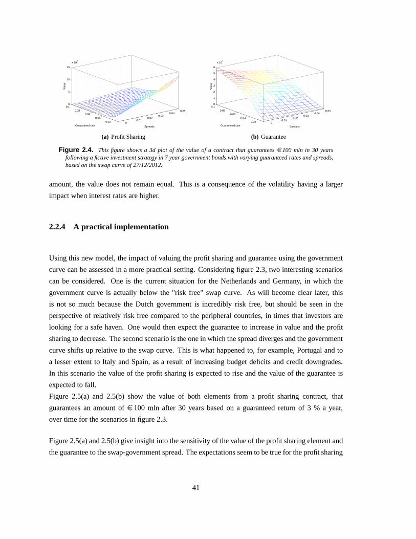
00.01

0.020.03

0.040.05

0.020.04

0.060.08

0.10

5

10

15

x 107

SpreadsGuaranteed rate

Val

ue

(a) Profit Sharing

00.01

0.020.03

0.040.05

0.020.04

0.060.08

0.10

1

2

3

4

5

6

x 107

SpreadsGuaranteed rate

Val

ue

(b) Guarantee

Figure 2.4. This figure shows a 3d plot of the value of a contract that guaranteese 100 mln in 30 yearsfollowing a fictive investment strategy in 7 year governmentbonds with varying guaranteed rates and spreads,based on the swap curve of 27/12/2012.

amount, the value does not remain equal. This is a consequence of the volatility having a larger

impact when interest rates are higher.

2.2.4 A practical implementation

Using this new model, the impact of valuing the profit sharingand guarantee using the government

curve can be assessed in a more practical setting. Considering figure 2.3, two interesting scenarios

can be considered. One is the current situation for the Netherlands and Germany, in which the

government curve is actually below the "risk free" swap curve. As will become clear later, this

is not so much because the Dutch government is incredibly risk free, but should be seen in the

perspective of relatively risk free compared to the peripheral countries, in times that investors are

looking for a safe haven. One would then expect the guaranteeto increase in value and the profit

sharing to decrease. The second scenario is the one in which the spread diverges and the government

curve shifts up relative to the swap curve. This is what happened to, for example, Portugal and to

a lesser extent to Italy and Spain, as a result of increasing budget deficits and credit downgrades.

In this scenario the value of the profit sharing is expected torise and the value of the guarantee is

expected to fall.

Figure 2.5(a) and 2.5(b) show the value of both elements froma profit sharing contract, that

guarantees an amount ofe 100 mln after 30 years based on a guaranteed return of 3 % a year,

over time for the scenarios in figure 2.3.

Figure 2.5(a) and 2.5(b) give insight into the sensitivity of the value of the profit sharing element and

the guarantee to the swap-government spread. The expectations seem to be true for the profit sharing

41

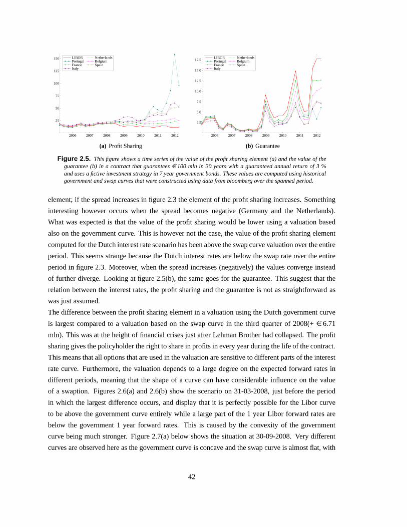
LIBOR Portugal France Italy

Netherlands Belgium Spain

2006 2007 2008 2009 2010 2011 2012

25

50

75

100

125

150 LIBOR Portugal France Italy

Netherlands Belgium Spain

(a) Profit Sharing

LIBOR Portugal France Italy

Netherlands Belgium Spain

2006 2007 2008 2009 2010 2011 2012

2.5

5.0

7.5

10.0

12.5

15.0

17.5LIBOR Portugal France Italy

Netherlands Belgium Spain

(b) Guarantee

Figure 2.5. This figure shows a time series of the value of the profit sharing element (a) and the value of theguarantee (b) in a contract that guaranteese 100 mln in 30 years with a guaranteed annual return of 3 %and uses a fictive investment strategy in 7 year government bonds. These values are computed using historicalgovernment and swap curves that were constructed using datafrom bloomberg over the spanned period.

element; if the spread increases in figure 2.3 the element of the profit sharing increases. Something

interesting however occurs when the spread becomes negative (Germany and the Netherlands).

What was expected is that the value of the profit sharing wouldbe lower using a valuation based

also on the government curve. This is however not the case, the value of the profit sharing element

computed for the Dutch interest rate scenario has been abovethe swap curve valuation over the entire

period. This seems strange because the Dutch interest ratesare below the swap rate over the entire

period in figure 2.3. Moreover, when the spread increases (negatively) the values converge instead

of further diverge. Looking at figure 2.5(b), the same goes for the guarantee. This suggest that the

relation between the interest rates, the profit sharing and the guarantee is not as straightforward as

was just assumed.

The difference between the profit sharing element in a valuation using the Dutch government curve

is largest compared to a valuation based on the swap curve in the third quarter of 2008(+e 6.71

mln). This was at the height of financial crises just after Lehman Brother had collapsed. The profit

sharing gives the policyholder the right to share in profits in every year during the life of the contract.

This means that all options that are used in the valuation aresensitive to different parts of the interest

rate curve. Furthermore, the valuation depends to a large degree on the expected forward rates in

different periods, meaning that the shape of a curve can haveconsiderable influence on the value

of a swaption. Figures 2.6(a) and 2.6(b) show the scenario on31-03-2008, just before the period

in which the largest difference occurs, and display that it is perfectly possible for the Libor curve

to be above the government curve entirely while a large part of the 1 year Libor forward rates are

below the government 1 year forward rates. This is caused by the convexity of the government

curve being much stronger. Figure 2.7(a) below shows the situation at 30-09-2008. Very different

curves are observed here as the government curve is concave and the swap curve is almost flat, with

42

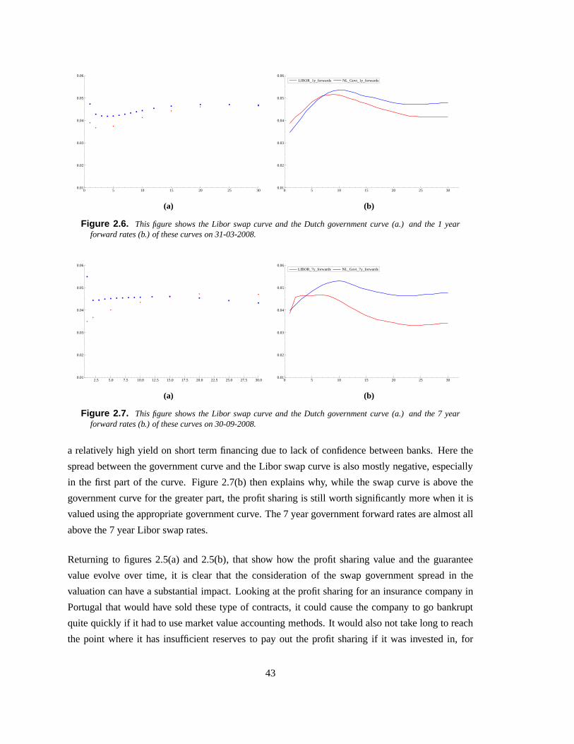
0 5 10 15 20 25 300.01

0.02

0.03

0.04

0.05

0.06

(a)

LIBOR_1y_forwards NL_Govt_1y_forwards

0 5 10 15 20 25 300.01

0.02

0.03

0.04

0.05

0.06LIBOR_1y_forwards NL_Govt_1y_forwards

(b)

Figure 2.6. This figure shows the Libor swap curve and the Dutch government curve (a.) and the 1 yearforward rates (b.) of these curves on 31-03-2008.

2.5 5.0 7.5 10.0 12.5 15.0 17.5 20.0 22.5 25.0 27.5 30.00.01

0.02

0.03

0.04

0.05

0.06

(a)

LIBOR_7y_forwards NL_Govt_7y_forwards

0 5 10 15 20 25 300.01

0.02

0.03

0.04

0.05

0.06LIBOR_7y_forwards NL_Govt_7y_forwards

(b)

Figure 2.7. This figure shows the Libor swap curve and the Dutch government curve (a.) and the 7 yearforward rates (b.) of these curves on 30-09-2008.

a relatively high yield on short term financing due to lack of confidence between banks. Here the

spread between the government curve and the Libor swap curveis also mostly negative, especially

in the first part of the curve. Figure 2.7(b) then explains why, while the swap curve is above the

government curve for the greater part, the profit sharing is still worth significantly more when it is

valued using the appropriate government curve. The 7 year government forward rates are almost all

above the 7 year Libor swap rates.

Returning to figures 2.5(a) and 2.5(b), that show how the profit sharing value and the guarantee

value evolve over time, it is clear that the consideration ofthe swap government spread in the

valuation can have a substantial impact. Looking at the profit sharing for an insurance company in

Portugal that would have sold these type of contracts, it could cause the company to go bankrupt

quite quickly if it had to use market value accounting methods. It would also not take long to reach

the point where it has insufficient reserves to pay out the profit sharing if it was invested in, for

43

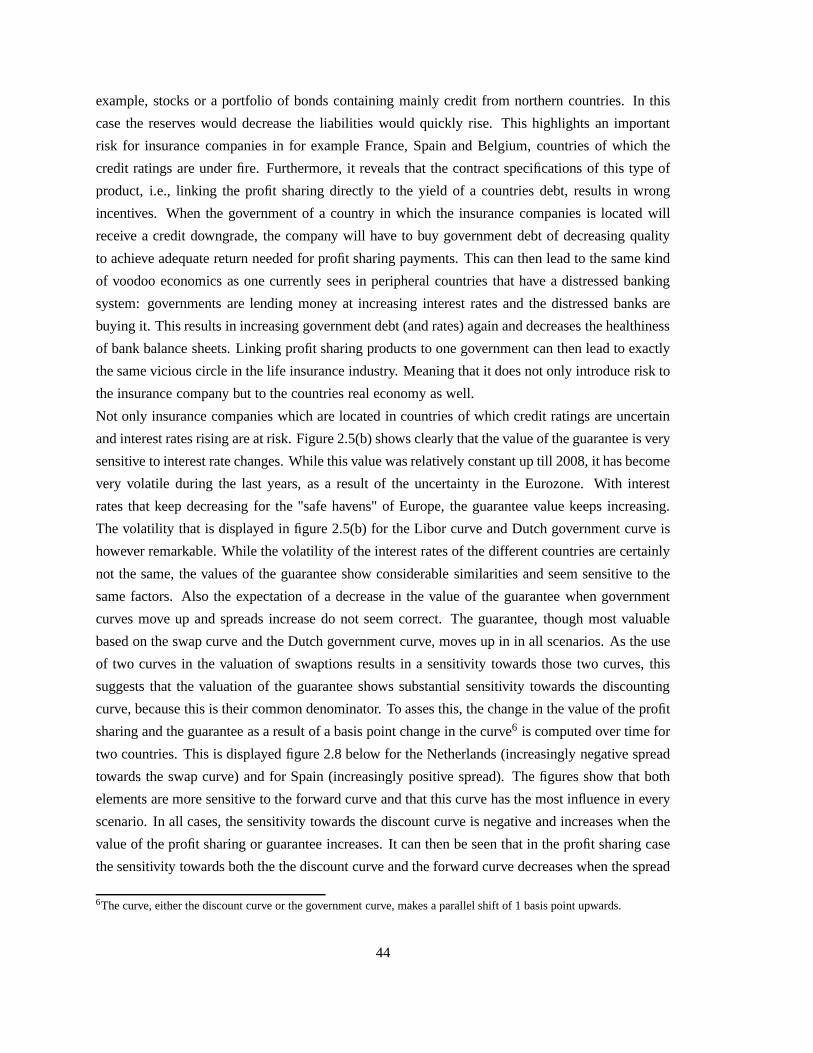
example, stocks or a portfolio of bonds containing mainly credit from northern countries. In this

case the reserves would decrease the liabilities would quickly rise. This highlights an important

risk for insurance companies in for example France, Spain and Belgium, countries of which the

credit ratings are under fire. Furthermore, it reveals that the contract specifications of this type of

product, i.e., linking the profit sharing directly to the yield of a countries debt, results in wrong

incentives. When the government of a country in which the insurance companies is located will

receive a credit downgrade, the company will have to buy government debt of decreasing quality

to achieve adequate return needed for profit sharing payments. This can then lead to the same kind

of voodoo economics as one currently sees in peripheral countries that have a distressed banking

system: governments are lending money at increasing interest rates and the distressed banks are

buying it. This results in increasing government debt (and rates) again and decreases the healthiness

of bank balance sheets. Linking profit sharing products to one government can then lead to exactly

the same vicious circle in the life insurance industry. Meaning that it does not only introduce risk to

the insurance company but to the countries real economy as well.

Not only insurance companies which are located in countriesof which credit ratings are uncertain

and interest rates rising are at risk. Figure 2.5(b) shows clearly that the value of the guarantee is very

sensitive to interest rate changes. While this value was relatively constant up till 2008, it has become

very volatile during the last years, as a result of the uncertainty in the Eurozone. With interest

rates that keep decreasing for the "safe havens" of Europe, the guarantee value keeps increasing.

The volatility that is displayed in figure 2.5(b) for the Libor curve and Dutch government curve is

however remarkable. While the volatility of the interest rates of the different countries are certainly

not the same, the values of the guarantee show considerable similarities and seem sensitive to the

same factors. Also the expectation of a decrease in the valueof the guarantee when government

curves move up and spreads increase do not seem correct. The guarantee, though most valuable

based on the swap curve and the Dutch government curve, movesup in in all scenarios. As the use

of two curves in the valuation of swaptions results in a sensitivity towards those two curves, this

suggests that the valuation of the guarantee shows substantial sensitivity towards the discounting

curve, because this is their common denominator. To asses this, the change in the value of the profit

sharing and the guarantee as a result of a basis point change in the curve6 is computed over time for

two countries. This is displayed figure 2.8 below for the Netherlands (increasingly negative spread

towards the swap curve) and for Spain (increasingly positive spread). The figures show that both

elements are more sensitive to the forward curve and that this curve has the most influence in every

scenario. In all cases, the sensitivity towards the discount curve is negative and increases when the

value of the profit sharing or guarantee increases. It can then be seen that in the profit sharing case

the sensitivity towards both the the discount curve and the forward curve decreases when the spread

6The curve, either the discount curve or the government curve, makes a parallel shift of 1 basis point upwards.

44

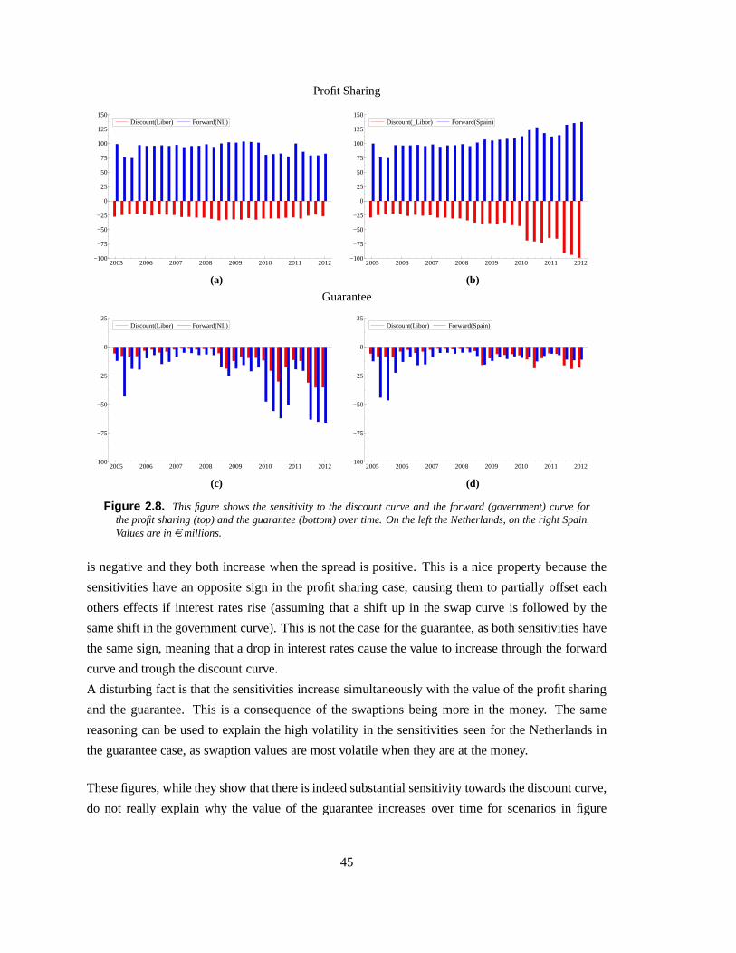
Profit Sharing

Discount(Libor) Forward(NL)

2005 2006 2007 2008 2009 2010 2011 2012−100

−75

−50

−25

0

25

50

75

100

125

150Discount(Libor) Forward(NL)

(a)

Discount(_Libor) Forward(Spain)

2005 2006 2007 2008 2009 2010 2011 2012−100

−75

−50

−25

0

25

50

75

100

125

150Discount(_Libor) Forward(Spain)

(b)

Guarantee

Discount(Libor) Forward(NL)

2005 2006 2007 2008 2009 2010 2011 2012−100

−75

−50

−25

0

25Discount(Libor) Forward(NL)

(c)

Discount(Libor) Forward(Spain)

2005 2006 2007 2008 2009 2010 2011 2012−100

−75

−50

−25

0

25Discount(Libor) Forward(Spain)

(d)

Figure 2.8. This figure shows the sensitivity to the discount curve and the forward (government) curve forthe profit sharing (top) and the guarantee (bottom) over time. On the left the Netherlands, on the right Spain.Values are inemillions.

is negative and they both increase when the spread is positive. This is a nice property because the

sensitivities have an opposite sign in the profit sharing case, causing them to partially offset each

others effects if interest rates rise (assuming that a shiftup in the swap curve is followed by the

same shift in the government curve). This is not the case for the guarantee, as both sensitivities have

the same sign, meaning that a drop in interest rates cause thevalue to increase through the forward

curve and trough the discount curve.

A disturbing fact is that the sensitivities increase simultaneously with the value of the profit sharing

and the guarantee. This is a consequence of the swaptions being more in the money. The same

reasoning can be used to explain the high volatility in the sensitivities seen for the Netherlands in

the guarantee case, as swaption values are most volatile when they are at the money.

These figures, while they show that there is indeed substantial sensitivity towards the discount curve,

do not really explain why the value of the guarantee increases over time for scenarios in figure

45

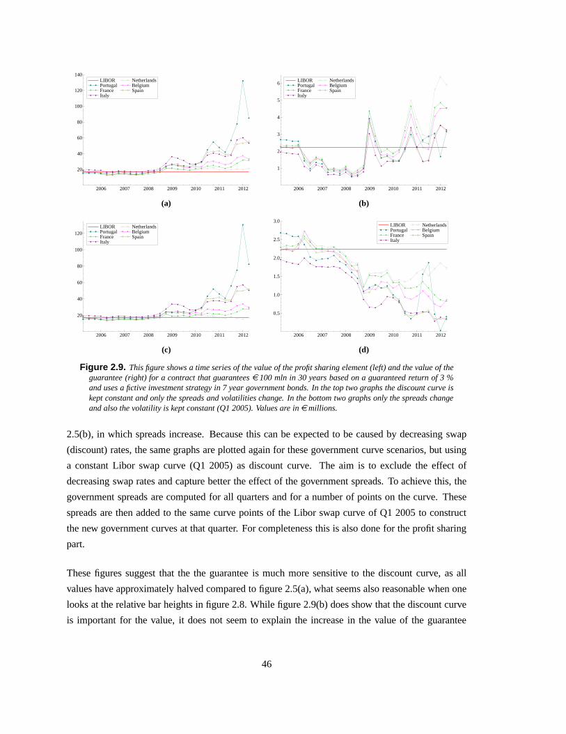
LIBOR Portugal France Italy

Netherlands Belgium Spain

2006 2007 2008 2009 2010 2011 2012

20

40

60

80

100

120

140LIBOR Portugal France Italy

Netherlands Belgium Spain

(a)

LIBOR Portugal France Italy

Netherlands Belgium Spain

2006 2007 2008 2009 2010 2011 2012

1

2

3

4

5

6LIBOR Portugal France Italy

Netherlands Belgium Spain

(b)

LIBOR Portugal France Italy

Netherlands Belgium Spain

2006 2007 2008 2009 2010 2011 2012

20

40

60

80

100

120LIBOR Portugal France Italy

Netherlands Belgium Spain

(c)

LIBOR Portugal France Italy

Netherlands Belgium Spain

2006 2007 2008 2009 2010 2011 2012

0.5

1.0

1.5

2.0

2.5

3.0LIBOR Portugal France Italy

Netherlands Belgium Spain

(d)

Figure 2.9. This figure shows a time series of the value of the profit sharing element (left) and the value of theguarantee (right) for a contract that guaranteese 100 mln in 30 years based on a guaranteed return of 3 %and uses a fictive investment strategy in 7 year government bonds. In the top two graphs the discount curve iskept constant and only the spreads and volatilities change.In the bottom two graphs only the spreads changeand also the volatility is kept constant (Q1 2005). Values are inemillions.

2.5(b), in which spreads increase. Because this can be expected to be caused by decreasing swap

(discount) rates, the same graphs are plotted again for these government curve scenarios, but using

a constant Libor swap curve (Q1 2005) as discount curve. The aim is to exclude the effect of

decreasing swap rates and capture better the effect of the government spreads. To achieve this, the

government spreads are computed for all quarters and for a number of points on the curve. These

spreads are then added to the same curve points of the Libor swap curve of Q1 2005 to construct

the new government curves at that quarter. For completenessthis is also done for the profit sharing

part.

These figures suggest that the the guarantee is much more sensitive to the discount curve, as all

values have approximately halved compared to figure 2.5(a),what seems also reasonable when one

looks at the relative bar heights in figure 2.8. While figure 2.9(b) does show that the discount curve

is important for the value, it does not seem to explain the increase in the value of the guarantee

46

over a period in which spreads increase. Figure 2.9(b) does suggest that from the fourth quarter in

2009 something changes in the way interest rate swaptions were valued as everything shifts up. If

the decreasing discount rates do not explain this, the only thing that can is the volatility which is

used in pricing these swaptions or, as we saw earlier, the shape of the curves. Lastly then, figure

2.9(c) and 2.9(d) show the values when only the spreads vary over time. The graphs takes on a

completely different shape what makes clear that the volatility has a substantial influence on the

value of the guarantee. The effect of the spreads is far more clear from this graph, as one can see

that the value of the guarantee decreases for the countries of which the spreads increased since the

Eurozones sovereign crises started and the value increasessince 2010 for the Netherlands (negative

spread towards the swap curve). The drop in value during the burst of the housing bubble (Q3 2007

- Q3 2008) is explained by government, showing an increased negative spread.7 As from the start

of the financial crises (fall of Lehman in Q3 2008) the spreadsof the peripheral countries in Europe

increased slightly but the government curve of the "safe" countries stayed below the swap curve,

resulting in respectively a decrease and increase in the value of the guarantee in these countries.

During Q3 of 2009 these spreads slightly converged again until the sovereign debt crises in Europe

started that made them diverge again. The directions in figure 2.9(d) clearly show that increasing

spreads generally decrease the value of the guarantee and increasing negative spreads increase the

value. Exactly opposite of the profit sharing case. The values of the guarantee for Portugal however

seem to disagree with this during Q1 and Q2 of 2011, showing a significant increase while spreads

also increased. This is due to a shift in the curve, as the interest rates of low maturities increased

quickly due to a lot of uncertainty over shorter horizons while longer term yields reacted less. This

resulted in lower forward rates further away, increasing the value of the swaptions. The hops that are

observed in the profit sharing series of Portugal in figure 2.9(c), where the value suddenly increases

and decreases, are also explained by the spreads. Looking atthose periods in figure 2.3 one sees that

all interest rates move parallel to the swap curve but this correlation is broken for the Portuguese

interest rates.

Figure 2.9 showed that both the spread and the volatility have an influence on the value of the

guarantee and on the value of the profit sharing. The shape of the curve however still influences the

values as well and this distorts a transparent observation of the relative effect that the volatility and

spread have. To overcome this, figure 2.10 shows the relationclearer, because all curves are kept

flat and only the spreads and volatility vary. As expected, both the value of the guarantee and the

value of the profit sharing increases when volatility rises.The values react oppositely to expanding

spreads; profit sharing increases, guarantee decreases. Aninteresting observation, that agrees with

the big differences between figures 2.9(b) and 2.9(d), is that the value of the guarantee is relatively

7Until the financial crises all government yields were below the Libor swap curve, as governments were consideredentirely risk free.

47

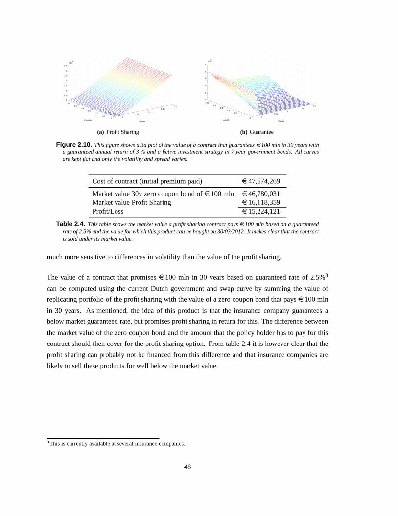
00.05

0.10.15

0.2

00.1

0.20.3

0.40.5

0.6

0

0.5

1

1.5

2

2.5

3

3.5

x 108

SpreadVolatility

(a) Profit Sharing

00.05

0.10.15

0.2

00.1

0.20.3

0.40.5

0.6

0

1

2

3

4

5

x 107

SpreadVolatility

(b) Guarantee

Figure 2.10. This figure shows a 3d plot of the value of a contract that guaranteese 100 mln in 30 years witha guaranteed annual return of 3 % and a fictive investment strategy in 7 year government bonds. All curvesare kept flat and only the volatility and spread varies.

Cost of contract (initial premium paid) e 47,674,269

Market value 30y zero coupon bond ofe 100 mln e 46,780,031Market value Profit Sharing e 16,118,359Profit/Loss e 15,224,121-

Table 2.4. This table shows the market value a profit sharing contract payse 100 mln based on a guaranteedrate of 2.5% and the value for which this product can be boughton 30/03/2012. It makes clear that the contractis sold under its market value.

much more sensitive to differences in volatility than the value of the profit sharing.

The value of a contract that promisese 100 mln in 30 years based on guaranteed rate of 2.5%8

can be computed using the current Dutch government and swap curve by summing the value of

replicating portfolio of the profit sharing with the value ofa zero coupon bond that payse 100 mln

in 30 years. As mentioned, the idea of this product is that theinsurance company guarantees a

below market guaranteed rate, but promises profit sharing inreturn for this. The difference between

the market value of the zero coupon bond and the amount that the policy holder has to pay for this

contract should then cover for the profit sharing option. From table 2.4 it is however clear that the

profit sharing can probably not be financed from this difference and that insurance companies are

likely to sell these products for well below the market value.

8This is currently available at several insurance companies.

48

2.3 Summary

In summary this chapter has shown that there are two ways in which these profit sharing products can

be modeled. Though both should result in the same value, one explicitly models the profit sharing

and one explicitly models the guarantee. The value of both elements was subsequently analyzed for

scenarios of varying swap-government spreads, using a valuation method that considers both the

government rates and the swap rates. This showed that there is indeed significant exposure towards

both curves and that the value of the profit sharing is extremely sensitive to swap government

spreads. This can lead to perverse situations in which insurance companies are almost obligated

to invest in lower quality government bonds in order to be able to pay out the profit sharing.

The value of the guarantee is low compared to the profit sharing but is relatively more sensitive

towards the discount curve and to fluctuations in volatility. Furthermore, it has become clear that

the value of both elements are very sensitive to the shape of the curve, which essentially determines

the value of the swaptions.

Although guarantee values are generally lower than profit sharing values, the risks involved with the

guarantee might actually be higher. Profit sharing should inessence not be a problem because, if

yields go up, the insurance companies can invest in the bonds. Except for the (possibly substantial)

risk of a counterparty defaulting, the company can then share the profits with the policyholder.9 The

guarantee might however be more dangerous, as this means that there are no bonds of the desired

credit rating that yield a return high enough to cover the guarantee. This means that following the

investment policy that specifies how the profit sharing is determined is not an option and investments

in theoretically riskier assets, yielding more, have to be made.

9Book value would then coincide, using market based accounting rules there would however still be a gap between assetsand liabilities.

49

Chapter 3

Hedging strategies

Traditionally risk management in the life insurance industry has always relied on long term

expectations about longevity, inflation, investment returns and regulatory frameworks. This resulted

in the common view on this industry being one of the most stable and reliable. With the introduction

of an increased amount of complex products and a regulatory framework relying more on market

based valuation techniques, this era belongs to the past. Especially now, as markets are more volatile

than ever.

Combining the long term nature of the insurance industry with market consisting valuation

and increasingly complex products creates a challenging environment for solvency and risk

management. This chapter will therefore discuss several basic strategies that can be applied in

mitigating the risks that profit sharing products introduce. The main question that will be answered

is how insurers can hedge the risks on their balance sheet which policyholders seek protection from.

This essentially entails hedging the two components that underlie the existence of these products:

1) a guaranteed return somewhere in the future and, 2) profit from high interest rates.

The first section will introduce the framework that will be used to evaluate all hedging strategies and

will discuss some related literature as well. Section 3.2 will discuss various products and strategies

that can be used to mitigate risks. The proposed strategies will then be evaluated in section 3.3 to

asses the effectiveness in different scenarios. Finally, in section 3.4 the performance of the strategies

are assessed based on a backtest using historical data on European countries interest rates. The

chapter will again conclude with a short summary of the main results.

50

3.1 Framework

Though the main emphasis has definitely been on the fair valuation of the embedded options

that are present in the products that life insurers sell, literature on risk management practices for

them is also available. Originally risk management in this industry followed the passive actuaries

approach of holding enough risk free assets to meet the liabilities with high probability. This has

however become hard due to the nature of the products which are currently available. Another

approach is to use results of finance to compute the fair valueof these contracts and match the

liabilities by rebalancing positions in different basic asset classes. But most of the literature that

is specifically on hedging life insurance products use risk minimizing strategies. For this, the

results of Föllmer and Sondermann (1986) are often applied,whom proved the existence of a unique

risk minimizing hedging strategy for any square-integrable contingent claim with a fixed maturity.

This approach aims to minimize total discounted profits and losses. Coleman et al. (2003) discuss

piece wise linear risk minimizing strategies based on localrisk minimization (match final value and

minimize intermediate cash flows individually) as an alternative, avoiding computationally difficult

dynamic stochastic programming problems encountered in minimizing over all periods. They find

that this method has a high probability of outperforming thequadratic programming model under the

assumption of a complete market. Subsequent research adds by introducing mortality risk (Moller

(2001)) or considering more realistic price, market and interest rate modeling. A useful introduction

and summary of the performance of several strategies, e.g. delta hedging, static hedging, risk

minimizing strategies and the modeling of mortality and financial risk is given by Nteukam et al.

(2011).

However, the amount of literature on hedging strategies is still limited and remains very theoretical,

especially for the type profit sharing products discussed here. The work done by Pelsser (2008)

is probably most related to the approach that will be taken inthis thesis. He discussed hedging

the minimum guarantee in British Guaranteed Annuity Options using a static portfolio of receiver

swaptions and found this to be effective based on historicaldata. An important difference between

all previous literature and this work is that all products are "directly" unit-linked. This means that

the hedging strategies that are discussed focus all on mitigating the risks introduced by the guarantee

given to the policyholder. The risks introduced by the otherelement, being the profit sharing, are

not really considered because this can be mitigated quite simply by investing in the asset to which

it is linked, assuming that this is possible.

It has been made clear that the profit sharing products in the Netherlands are in general not directly

linked to an asset in which one can invest because the u-rate is not traded on financial markets. It

was revealed in the last chapter that an important factor to the value of these products is the credit

51

spread between the Libor swap rate and the government yields, and that neglecting this feature can

amount in substantial errors in the valuation of it. As a consequence the consideration of this spread

in determining risk mitigating strategies is essential to achieve required effectiveness. Therefore, in

contrast to earlier research, the downside risk will be quickly dealt with by the use of a zero coupon

bond that returns the guaranteed amount. The focus will thenmainly be on what strategies can be

used to hedge the profit sharing and the swap-government spread that was discussed in chapter 2.

3.2 Instruments & Strategies

The profit sharing product used here will be the one that is considered throughout this thesis; it

promisese 100 mln in 30 years based on some guaranteed rate and uses a fictive investment policy

that is characterized by investing in 7 year bonds with coupons equal to the then prevailing u-rate.

Figure 2.8 in chapter 2 showed that the value of the profit sharing in this product is sensitive to two

interest rate curves. The sensitivity is measured in BPV (basis point value) which is one of two,

the other one being duration, measures which are most often used in assessing sensitivity to interest

rate changes. BPV measures exactly what is in the name, the change in value when the interest rate

goes up by one basis point (0.01%). Duration is a mathematical expression introduced by Macaulay

(1910) that captures the weighted average term to maturity of a fixed income product by considering

all cash flows associated with the product. The modified duration is a linear approximation for the

percentage change in value of a fixed income product when the yield changes by one percent and

is closely related to the duration and BPV. Throughout this chapter the measure that will be used to

asses sensitivity will be BPV.

The interest rate sensitivity of the value of the guarantee,modeled by a zero coupon bond paying

e 100 mln, can be visualized in a similar way as the profit sharing in figure 2.8. What is not

displayed in figure 2.8, but is essential in determining hedging strategies, is that the sensitivity

varies between different part of the interest rate curve. This means that every bar in figure 2.8 can

be split up in a sensitivity to the parts (yields computed from traded bonds with different maturities)

that are used to build the curve. These parts are often calledbuckets, because sensitivity to a range

of yields is usually hedged by only a few instruments, the sensitivities are therefore "bucketed".

When this is done for a contract with guaranteed rate of 2.5% it reveals that the 7y and 30y point

influence the value most. This is due to the zero coupon bond that is only sensitive to this point

(negatively) but also due to the profit sharing as the value issensitive (positively) to the government

curve.

From this point on the hedge for the guaranteed amount ofe 100 mln will not be discussed further

52

and the focus will be solely on the profit sharing part.

3.2.1 Delta hedging

Using the sensitivities that were just discussed one can compose an offsetting position with

sensitivities that have exactly the opposite sign using theproducts that were also available to

construct the curve. This would result in a portfolio of cash, swaps and zero coupon government

bonds that should equal the value of profit sharing if there isa change of one basis point in the

curve. The swap hedge should be a position in receiver swaps1 that increases in value when swap

rates decrease, as the value of the product increases when discount rates drop and vice versa. This

hedge would then also require a short position in governmentbonds because profit sharing increases

when yields increase and a short position increases when this happens as well. This might sound

counter intuitive as the amount of profit sharing increases when government bond yields rise (u-rates

increase). In the first place the aim should however not be to replicate the cash flows exactly

but the market value itself. If government bond yields rise,the hedge value increases and the

holder of the hedge can finance the risen promised profit sharing from this. This actually reveals

the difference in contract specification between a profit sharing contract with a guarantee and a

unit-linked contract. In a unit-linked product that would have promised the return on a portfolio of

government bonds, the insurer could hedge this by investingin this portfolio and the risks will be

for the policyholder. For the profit sharing product, the situation is exactly opposite as, when the

insurer promises the return on the government bonds and the government defaults, the insurer still

has to pay the guarantee but has no underlying asset to pay it with. Hence the insurer bears the risk.

This means that for a unit-linked portfolio the value of the investments, when done according to the

specification of the product, always exactly matches the liabilities value. But for a profit sharing

product with a guarantee, the market value of the product will generally differ from the specified

investments of the fictitious investments. The easiest way to see this is considering a downgrade

of the government. The yields will rise, making the investments worth less (this would be a bad

scenario for a policyholder with a unit-linked product), but the u-rates rise, increasing the value of

the profit sharing (so a positive scenario for a policyholderwith a profit sharing product).

It is clear that the aim of a hedge consisting of swaps and zerocoupon bonds is to mimic the

optional character of the profit sharing by using a portfolioof linear products. This is in fact similar

to applying a delta hedging strategy. The selling of profit sharing is in a way equal to selling put

options on government bonds as the value of these put optionsincrease when yields go up. To delta

1It can well be that the portfolio consists of both payer and receiver swaps, this statement aims at the net position.

53

hedge a put option one has to sell the underlying as the options go "in-the-money".2

3.2.2 Delta hedging and CDS

Though in theory delta hedging can be applied to hedge any derivative, the real world has different

rules that sadly make this strategy difficult or impossible to implement. The long maturities of the

insurance products make a delta hedging strategy difficult to apply and another practical limitation

is that delta hedging requires the selling of bonds. The strategy would then require the selling

of sovereign debt, this increases yields and therefore results a vicious circle.3 Furthermore delta

hedging requires continuous rebalancing, imposing additional costs.

In chapter 2 the importance of modeling the swap-governmentspread was emphasized. It was

discussed here that the Dutch government yield can theoretically be split up in a credit spread part

and a risk free (Libor) part. This is in line with the explanation given above that the selling of profit

sharing based on u-yield results in exposure to default risk. It would mean that the short position in

government bonds can be seen as a short position in Libor and exposure to a product that increases

in value when the credit spread rises. This exposure can be found in CDS (Credit Default Swap)

contracts, which, when having a long position, protects theinvestor.

3.2.2.1 Credit Default Swap

In a credit default swap two parties enter into an agreement that ends at at stated maturity or when a

"credit event" occurs. In this agreement one party (the insurance buyer) pays a fixed fee at the end

of every period until maturity of the contract and receives protection on some underlying in return

from the other other party (the insurance seller). Hence, this contract transfers the credit risk from

one party to another. The relevant underlying in this setting is a government bond but CDS contracts

are available for a wide range of fixed income products. The "credit events" that trigger payment

are specified in the contract. The most important ones, defined by the ISDA4, are :

- Failure to pay payments when they are due.

2In line with section 2.1 one could also delta hedge the product with receiver swaps and a long position in governmentbonds, not using a zero coupon bond. This is however not discussed here as this does not model the profit sharingexplicitly.

3There is in fact a draft law that poses limitations on the selling of sovereign debt products in some situations, seeDutch State Treasury Agency (2011)

4International Swaps and Derivatives Association

54

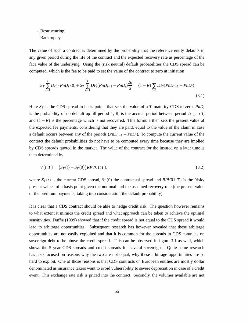
- Restructuring.

- Bankruptcy.

The value of such a contract is determined by the probabilitythat the reference entity defaults in

any given period during the life of the contract and the expected recovery rate as percentage of the

face value of the underlying. Using the (risk neutral) default probabilities the CDS spread can be

computed, which is the fee to be paid to set the value of the contract to zero at initiation

ST

T

∑i=1

DFi ·PnDi ·∆i +ST

T

∑i=1

DFi(PnDi−1−PnDi)∆i

2= (1−R)

T

∑i=1

DFi(PnDi−1−PnDi).

(3.1)

HereST is the CDS spread in basis points that sets the value of aT maturity CDS to zero,PnDi

is the probability of no default up till periodi , ∆i is the accrual period between periodTi−1 to Ti

and(1−R) is the percentage which is not recovered. This formula then sets the present value of

the expected fee payments, considering that they are paid, equal to the value of the claim in case

a default occurs between any of the periods (PnDi−1−PnDi). To compute the current value of the

contract the default probabilities do not have to be computed every time because they are implied

by CDS spreads quoted in the market. The value of the contractfor the insured on a later time is

then determined by

V(t,T) =(

ST(t)−ST(0))

RPV01(T), (3.2)

whereST(t) is the current CDS spread,ST(0) the contractual spread andRPV01(T) is the ’risky

present value" of a basis point given the notional and the assumed recovery rate (the present value

of the premium payments, taking into consideration the default probability).

It is clear that a CDS contract should be able to hedge credit risk. The question however remains

to what extent it mimics the credit spread and what approach can be taken to achieve the optimal

sensitivities. Duffie (1999) showed that if the credit spread is not equal to the CDS spread it would

lead to arbitrage opportunities. Subsequent research has however revealed that these arbitrage

opportunities are not easily exploited and that it is commonfor the spreads in CDS contracts on

sovereign debt to be above the credit spread. This can be observed in figure 3.1 as well, which

shows the 5 year CDS spreads and credit spreads for several sovereigns. Quite some research

has also focused on reasons why the two are not equal, why these arbitrage opportunities are so

hard to exploit. One of those reasons is that CDS contracts onEuropean entities are mostly dollar

denominated as insurance takers want to avoid vulnerability to severe depreciation in case of a credit

event. This exchange rate risk is priced into the contract. Secondly, the volumes available are not

55

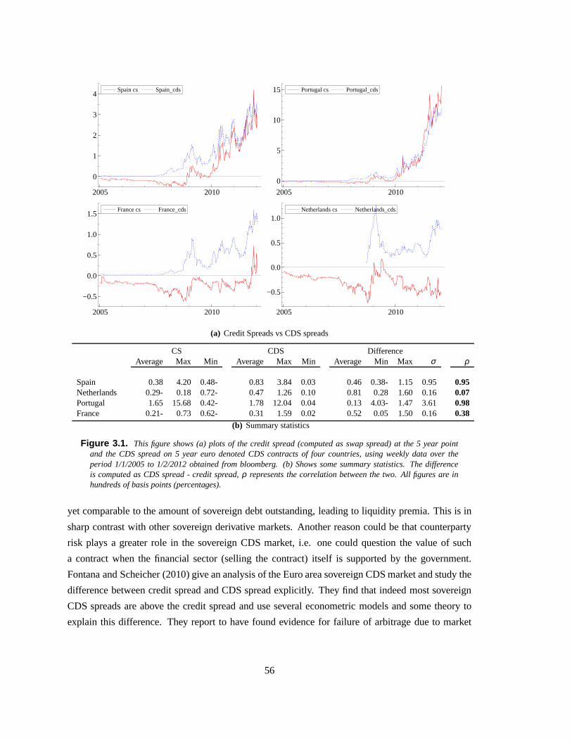
Spain cs Spain_cds

2005 2010

0

1

2

3

4Spain cs Spain_cds Portugal cs Portugal_cds

2005 2010

0

5

10

15 Portugal cs Portugal_cds

France cs France_cds

2005 2010

−0.5

0.0

0.5

1.0

1.5France cs France_cds Netherlands cs Netherlands_cds

2005 2010

−0.5

0.0

0.5

1.0Netherlands cs Netherlands_cds

(a) Credit Spreads vs CDS spreads

CS CDS DifferenceAverage Max Min Average Max Min Average Min Max σ ρ

Spain 0.38 4.20 0.48- 0.83 3.84 0.03 0.46 0.38- 1.15 0.950.95Netherlands 0.29- 0.18 0.72- 0.47 1.26 0.10 0.81 0.28 1.60 0.16 0.07Portugal 1.65 15.68 0.42- 1.78 12.04 0.04 0.13 4.03- 1.47 3.61 0.98France 0.21- 0.73 0.62- 0.31 1.59 0.02 0.52 0.05 1.50 0.160.38

(b) Summary statistics

Figure 3.1. This figure shows (a) plots of the credit spread (computed as swap spread) at the 5 year pointand the CDS spread on 5 year euro denoted CDS contracts of fourcountries, using weekly data over theperiod 1/1/2005 to 1/2/2012 obtained from bloomberg. (b) Shows some summary statistics. The differenceis computed as CDS spread - credit spread,ρ represents the correlation between the two. All figures are inhundreds of basis points (percentages).

yet comparable to the amount of sovereign debt outstanding,leading to liquidity premia. This is in

sharp contrast with other sovereign derivative markets. Another reason could be that counterparty

risk plays a greater role in the sovereign CDS market, i.e. one could question the value of such

a contract when the financial sector (selling the contract) itself is supported by the government.

Fontana and Scheicher (2010) give an analysis of the Euro area sovereign CDS market and study the

difference between credit spread and CDS spread explicitly. They find that indeed most sovereign

CDS spreads are above the credit spread and use several econometric models and some theory to

explain this difference. They report to have found evidencefor failure of arbitrage due to market

56

frictions and structural changes that limit traders to arbitrage differences away. Furthermore, they

do observe strong correlation between the two and conclude that price discovery shifts between

the derivative market and the bond market, depending in which the most informed investors are.

This could have implications for the hedging strategy as, when price discovery takes place in the

derivative market, the buying of CDS contracts leads to increased credit spread. This would then

lead to the same vicious circle as hedging by selling government bonds does. Something similar

would happen if bond traders would link a countries creditworthiness to the health of its financial

sector. If insurance companies would hold CDS contracts on sovereign debt that other financial

institutions have sold, this would lead to an increasing credit spread, resulting in a vicious circle

once more. Dieckmann and Plank (2010) and Ejsing and Lemke (2010) both study this subject

and do find some evidence on relations between the financial health of banks and sovereign CDS

spreads. Finally "flight to safety" can pose problems as thisdrives down government yields leading

to possibly negative credit spreads while CDS spreads do notshow this effect, increasing differences

between the two (this is illustrated for the Netherlands in figure 3.1(a)).

Though considering all these effects is important in designing hedge strategies, this is outside the

scope of this thesis. In the evaluation of the strategies theassumption is made that the CDS spread

is perfectly correlated with the credit spread. From the table in figure 3.1 one can see that the

correlations are very high in the times it matters (Portugaland Spain, but also during last year for

France), so the CDS spread definitely seems to capture jumps in creditworthiness and therefore the

assumption seems reasonable.

A hedge portfolio that consists of cash, swaps and a CDS contract should then create the right

exposures. In this portfolio the short position in government bonds from the last strategy is modeled

as a position in Libor (net payer swaps) and credit spread (long protection). The value of the CDS

contract is sensitive to both changes in the Libor swap curveand changes in the government curve.

If the Libor rates drop, the present value of future cash flowswill be higher but, more importantly,

the credit spread increases if the government rates remain equal. The CDS contract chosen is ideally

linked to the credit spread that influences the profit sharingmost, hence in this case seven year CDS

contracts will be considered.5 The notional amount insured is determined by the sensitivity of the

profit sharing to the government curve in the same way that thenotional amounts of the government

bonds are determined in the previous strategy. This strategy then requires an additional swap hedge

to hedge unwanted exposure to Libor swap rates introduced bythe CDS. Assuming that the CDS

spread is a deterministic function of the credit spread thisis visualized below by the use of a first

order Taylor expansion aroundPS(r f ,u), wherer f is the Libor rate and ,u= r f +csthe government

5One could also consider a hedge that uses multiple CDS contracts, this might result in better results for non-parallelcurve shifts. This is not done here because its expected to give only minor improvements in immunity while being lesscost efficient.

57

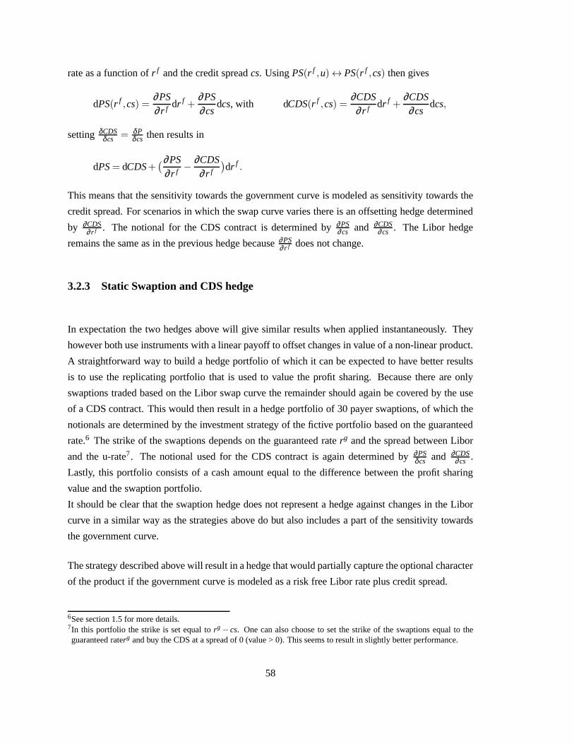
rate as a function ofr f and the credit spreadcs. UsingPS(r f ,u)↔ PS(r f ,cs) then gives

dPS(r f ,cs) =∂PS∂ r f dr f +

∂PS∂cs

dcs, with dCDS(r f ,cs) =∂CDS∂ r f dr f +

∂CDS∂cs

dcs,

settingδCDSδcs = δP

δcs then results in

dPS= dCDS+(∂PS

∂ r f − ∂CDS∂ r f

)

dr f .

This means that the sensitivity towards the government curve is modeled as sensitivity towards the

credit spread. For scenarios in which the swap curve varies there is an offsetting hedge determined

by ∂CDS∂ r f . The notional for the CDS contract is determined by∂PS

∂cs and ∂CDS∂cs . The Libor hedge

remains the same as in the previous hedge because∂PS∂ r f does not change.

3.2.3 Static Swaption and CDS hedge

In expectation the two hedges above will give similar results when applied instantaneously. They

however both use instruments with a linear payoff to offset changes in value of a non-linear product.

A straightforward way to build a hedge portfolio of which it can be expected to have better results

is to use the replicating portfolio that is used to value the profit sharing. Because there are only

swaptions traded based on the Libor swap curve the remaindershould again be covered by the use

of a CDS contract. This would then result in a hedge portfolioof 30 payer swaptions, of which the

notionals are determined by the investment strategy of the fictive portfolio based on the guaranteed

rate.6 The strike of the swaptions depends on the guaranteed raterg and the spread between Libor

and the u-rate7. The notional used for the CDS contract is again determined by ∂PSδcs and ∂CDS

∂cs .

Lastly, this portfolio consists of a cash amount equal to thedifference between the profit sharing

value and the swaption portfolio.

It should be clear that the swaption hedge does not representa hedge against changes in the Libor

curve in a similar way as the strategies above do but also includes a part of the sensitivity towards

the government curve.

The strategy described above will result in a hedge that would partially capture the optional character

of the product if the government curve is modeled as a risk free Libor rate plus credit spread.

6See section 1.5 for more details.7In this portfolio the strike is set equal torg − cs. One can also choose to set the strike of the swaptions equal to theguaranteed raterg and buy the CDS at a spread of 0 (value > 0). This seems to resultin slightly better performance.

58

3.2.4 Linear and non-linear hedge portfolios ignoring swap-government spread

For completeness, also the hedge portfolio that would be constructed when not considering varying

swap government spreads are evaluated. Under this assumption there is only sensitivity towards the

Libor curve because the u-rate is modeled asu = r f + cs, in which the spreadcs is fixed. Under

this assumption again a linear and a non-linear hedge can be constructed using respectively swaps or

swaptions. The linear hedge would consist of cash and swaps,in which the notionals are determined

by ∂P(r f )∂ r f . The non-linear hedge is just the replicating portfolio of Libor swaptions that is also used

in the previous hedge plus the difference between this valueand the profit sharing value in cash. The

CDS is not used to provide protection for varying swap government spreads, therefore it is expected

that this hedge will display a similar performance when the Libor and government curve move in

the same direction simultaneously.

3.3 Performance evaluation

To asses the performance of these strategies, first the difference between the value of the hedge

portfolio and the value of the profit sharing are considered for instantaneous parallel shifts in both

the Libor swap curve and the government curve.8. Subsequently, also the performance over a larger

time span will be evaluated.

3.3.1 Instantaneous performance

For this the Libor swap curve of 31/3/2012 will be used as standard reference and the government

curve is modeled by adding 20bp (basis points) as credit spread. In this scenario the value of the

profit sharing is approximatelye 15.8 mln. The shifts, in both swap and government curve, thatare

applied to this reference scenario are -100bp, -50bp, -20bp, -1bp , 0bp, 1bp, 20bp, 50bp and 100bp

resulting in a total of 81 scenarios. This means that the maximum credit spread will be 220bp in the

most extreme scenario.

8Constructing a hedge in this way should however result in a similar performance for non parallel shifts

59

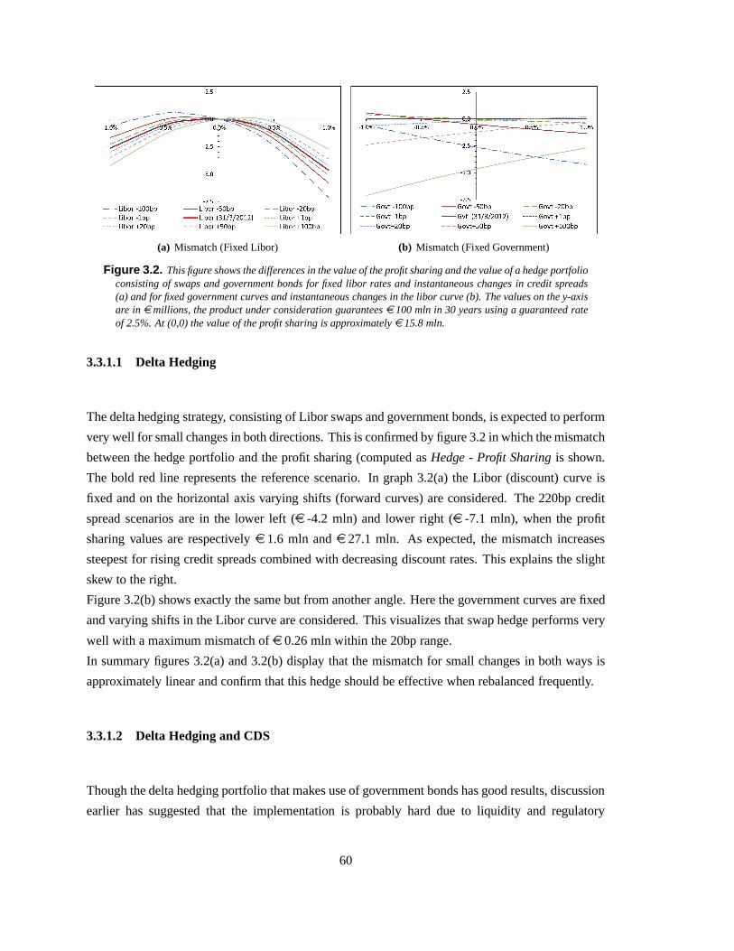
(a) Mismatch (Fixed Libor) (b) Mismatch (Fixed Government)

Figure 3.2. This figure shows the differences in the value of the profit sharing and the value of a hedge portfolioconsisting of swaps and government bonds for fixed libor rates and instantaneous changes in credit spreads(a) and for fixed government curves and instantaneous changes in the libor curve (b). The values on the y-axisare inemillions, the product under consideration guaranteese 100 mln in 30 years using a guaranteed rateof 2.5%. At (0,0) the value of the profit sharing is approximatelye 15.8 mln.

3.3.1.1 Delta Hedging

The delta hedging strategy, consisting of Libor swaps and government bonds, is expected to perform

very well for small changes in both directions. This is confirmed by figure 3.2 in which the mismatch

between the hedge portfolio and the profit sharing (computedasHedge - Profit Sharingis shown.

The bold red line represents the reference scenario. In graph 3.2(a) the Libor (discount) curve is

fixed and on the horizontal axis varying shifts (forward curves) are considered. The 220bp credit

spread scenarios are in the lower left (e -4.2 mln) and lower right (e -7.1 mln), when the profit

sharing values are respectivelye 1.6 mln ande 27.1 mln. As expected, the mismatch increases

steepest for rising credit spreads combined with decreasing discount rates. This explains the slight

skew to the right.

Figure 3.2(b) shows exactly the same but from another angle.Here the government curves are fixed

and varying shifts in the Libor curve are considered. This visualizes that swap hedge performs very

well with a maximum mismatch ofe 0.26 mln within the 20bp range.

In summary figures 3.2(a) and 3.2(b) display that the mismatch for small changes in both ways is

approximately linear and confirm that this hedge should be effective when rebalanced frequently.

3.3.1.2 Delta Hedging and CDS

Though the delta hedging portfolio that makes use of government bonds has good results, discussion

earlier has suggested that the implementation is probably hard due to liquidity and regulatory

60

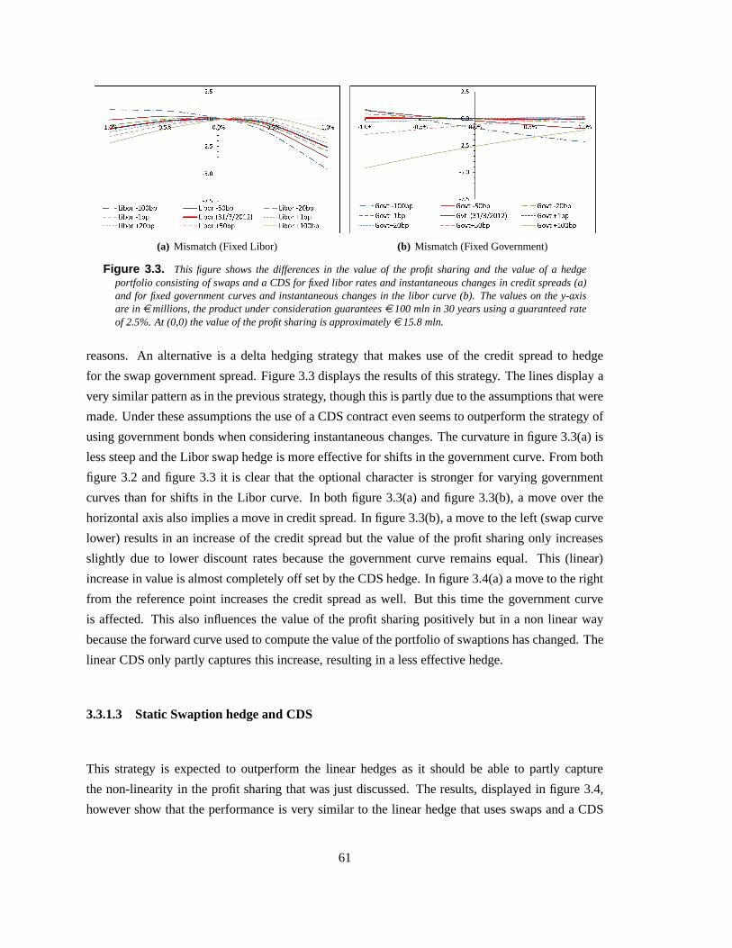
(a) Mismatch (Fixed Libor) (b) Mismatch (Fixed Government)

Figure 3.3. This figure shows the differences in the value of the profit sharing and the value of a hedgeportfolio consisting of swaps and a CDS for fixed libor rates and instantaneous changes in credit spreads (a)and for fixed government curves and instantaneous changes inthe libor curve (b). The values on the y-axisare inemillions, the product under consideration guaranteese 100 mln in 30 years using a guaranteed rateof 2.5%. At (0,0) the value of the profit sharing is approximatelye 15.8 mln.

reasons. An alternative is a delta hedging strategy that makes use of the credit spread to hedge

for the swap government spread. Figure 3.3 displays the results of this strategy. The lines display a

very similar pattern as in the previous strategy, though this is partly due to the assumptions that were

made. Under these assumptions the use of a CDS contract even seems to outperform the strategy of

using government bonds when considering instantaneous changes. The curvature in figure 3.3(a) is

less steep and the Libor swap hedge is more effective for shifts in the government curve. From both

figure 3.2 and figure 3.3 it is clear that the optional character is stronger for varying government

curves than for shifts in the Libor curve. In both figure 3.3(a) and figure 3.3(b), a move over the

horizontal axis also implies a move in credit spread. In figure 3.3(b), a move to the left (swap curve

lower) results in an increase of the credit spread but the value of the profit sharing only increases

slightly due to lower discount rates because the governmentcurve remains equal. This (linear)

increase in value is almost completely off set by the CDS hedge. In figure 3.4(a) a move to the right

from the reference point increases the credit spread as well. But this time the government curve

is affected. This also influences the value of the profit sharing positively but in a non linear way

because the forward curve used to compute the value of the portfolio of swaptions has changed. The

linear CDS only partly captures this increase, resulting ina less effective hedge.

3.3.1.3 Static Swaption hedge and CDS

This strategy is expected to outperform the linear hedges asit should be able to partly capture

the non-linearity in the profit sharing that was just discussed. The results, displayed in figure 3.4,

however show that the performance is very similar to the linear hedge that uses swaps and a CDS

61

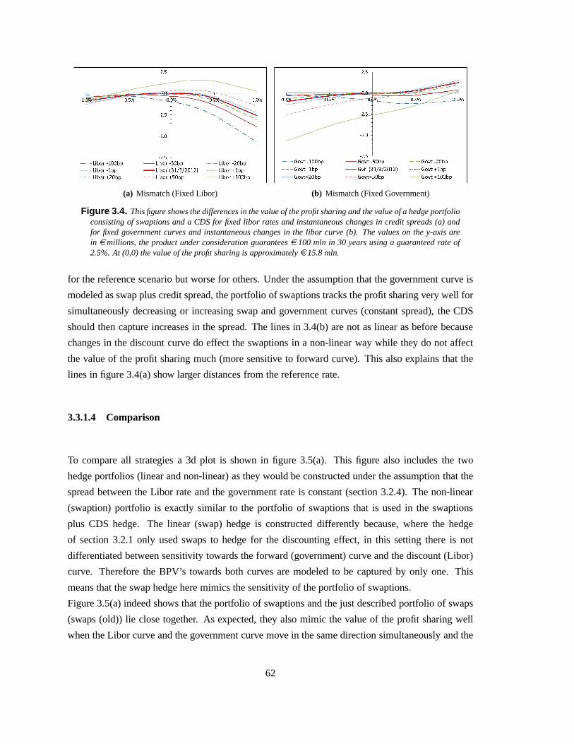
(a) Mismatch (Fixed Libor) (b) Mismatch (Fixed Government)

Figure 3.4. This figure shows the differences in the value of the profit sharing and the value of a hedge portfolioconsisting of swaptions and a CDS for fixed libor rates and instantaneous changes in credit spreads (a) andfor fixed government curves and instantaneous changes in thelibor curve (b). The values on the y-axis arein emillions, the product under consideration guaranteese 100 mln in 30 years using a guaranteed rate of2.5%. At (0,0) the value of the profit sharing is approximatelye 15.8 mln.

for the reference scenario but worse for others. Under the assumption that the government curve is

modeled as swap plus credit spread, the portfolio of swaptions tracks the profit sharing very well for

simultaneously decreasing or increasing swap and government curves (constant spread), the CDS

should then capture increases in the spread. The lines in 3.4(b) are not as linear as before because

changes in the discount curve do effect the swaptions in a non-linear way while they do not affect

the value of the profit sharing much (more sensitive to forward curve). This also explains that the

lines in figure 3.4(a) show larger distances from the reference rate.

3.3.1.4 Comparison

To compare all strategies a 3d plot is shown in figure 3.5(a). This figure also includes the two

hedge portfolios (linear and non-linear) as they would be constructed under the assumption that the

spread between the Libor rate and the government rate is constant (section 3.2.4). The non-linear

(swaption) portfolio is exactly similar to the portfolio ofswaptions that is used in the swaptions

plus CDS hedge. The linear (swap) hedge is constructed differently because, where the hedge

of section 3.2.1 only used swaps to hedge for the discountingeffect, in this setting there is not

differentiated between sensitivity towards the forward (government) curve and the discount (Libor)

curve. Therefore the BPV’s towards both curves are modeled to be captured by only one. This

means that the swap hedge here mimics the sensitivity of the portfolio of swaptions.

Figure 3.5(a) indeed shows that the portfolio of swaptions and the just described portfolio of swaps

(swaps (old)) lie close together. As expected, they also mimic the value of the profit sharing well

when the Libor curve and the government curve move in the samedirection simultaneously and the

62

credit spread remains equal. This is shown explicitly in figures 3.5(b) and 3.5(c). However, when

spreads do vary, these hedge portfolios display sensitivities that have the wrong sign, meaning that

the value of the hedge moves in the opposite way of the profit sharing value. Finance theory states

that such a scenario should not present itself as a government curve should always be on the same

level or above the risk free curve. Today it is however clear that in times of crises this is exactly

what happens: investors move away from riskier countries (increasing yields) and look for safe

havens, resulting in very low (sometimes negative) yields for these countries, while central banks

lower borrowing (lowering also Libor) rates to stimulate the economy. This stresses once more the

importance of acknowledging the fact that the value of theseprofit sharing products is determined

by two curves and that this should be used in designing and implementing effective hedge strategies

for profit sharing.

Figure 3.5 furthermore visualizes what has already been analyzed in the previous paragraphs and

confirms also by the numerics in the table that, when considering instantaneous changes, a linear

hedge consisting of swaps and a CDS seems to perform best.

63

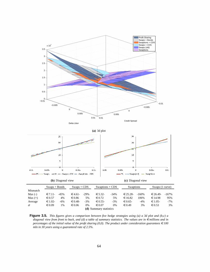
−0.01

−0.005

0

0.005

0.01

−0.01

−0.005

0

0.005

0.01

0

0.5

1

1.5

2

2.5

3

3.5

x 107

Credit SpreadDelta Libor

Profit SharingSwaps + BondsSwaptions + CDSSwaps + CDSSwaps (old)Swaptions

(a) 3d plot

(b) Diagonal view (c) Diagonal view

Swaps + Bonds Swaps + CDS Swaptions + CDS Swaptions Swaps (1 curve)MismatchMax (-) e 7.11- -45% e 4.61- -29% e 5.32- -34% e 25.28- -160% e 26.49- -167%Max (+) e 0.57 4% e 0.86 5% e 0.72 5% e 16.82 106% e 14.98 95%Average e 1.02- -6% e 0.48- -3% e 0.55- -3% e 0.65- -4% e 1.05- -7%σ e 0.09 1% e 0.06 0% e 0.07 0% e 0.49 3% e 0.53 3%

(d) Summary statistics

Figure 3.5. This figures gives a comparison between five hedge strategiesusing (a) a 3d plot and (b,c) adiagonal view from front to back, and (d) a table of summary statistics. The values are inemillions and inpercentages of the initial value of the profit sharing (0,0).The product under consideration guaranteese 100mln in 30 years using a guaranteed rate of 2.5%.

64

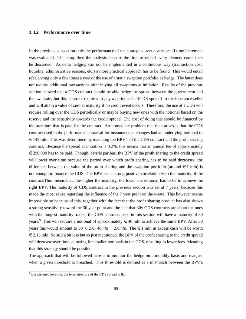
3.3.2 Performance over time

In the previous subsection only the performance of the strategies over a very small time increment

was evaluated. This simplified the analysis because the timeaspect of every element could then

be discarded. As delta hedging can not be implemented in a continuous way (transaction cost,

liquidity, administrative reasons, etc.) a more practicalapproach has to be found. This would entail

rebalancing only a few times a year or the use of a static swaption portfolio as hedge. The latter does

not require additional transactions after buying all swaptions at initiation. Results of the previous

section showed that a CDS contract should be able hedge the spread between the government and

the swaprate, but this contract requires to pay a periodic fee (CDS spread) to the insurance seller

and will attain a value of zero at maturity if no credit event occurs. Therefore, the use of a CDS will

require rolling over the CDS periodically or maybe buying new ones with the notional based on the

reserve and the sensitivity towards the credit spread. The cost of doing this should be financed by

the premium that is paid for the contract. An immediate problem that then arises is that the CDS

contract used in the performance appraisal for instantaneous changes had an underlying notional of

e 145 mln. This was determined by matching the BPV’s of the CDS contract and the profit sharing

contract. Because the spread at initiation is 0.2%, this means that an annual fee of approximately

e 290,000 has to be paid. Though, ceteris paribus, the BPV of the profit sharing to the credit spread

will lower over time because the period over which profit sharing has to be paid decreases, the

difference between the value of the profit sharing and the swaption portfolio (arounde 1 mln) is

not enough to finance the CDS. The BPV has a strong positive correlation with the maturity of the

contract.This means that, the higher the maturity, the lower the notional has to be to achieve the

right BPV. The maturity of CDS contract in the previous section was set at 7 years, because this

made the most sense regarding the influence of the 7 year pointon the u-rate. This however seems

impossible so because of this, together with the fact that the profit sharing product has also shown

a strong sensitivity toward the 30 year point and the fact that 30y CDS contracts are about the ones

with the longest maturity traded, the CDS contracts used in this section will have a maturity of 30

years.9 This will require a notional of approximatelye 46 mln to achieve the same BPV. After 30

years this would amount to 30·0.2%·46mln= 2.8mln. Thee 1 mln in excess cash will be worth

e 2.13 mln. So still a bit less but as just mentioned, the BPV of the profit sharing to the credit spread

will decrease over time, allowing for smaller notionals in the CDS, resulting in lower fees. Meaning

that this strategy should be possible.

The approach that will be followed here is to monitor the hedge on a monthly basis and readjust

when a given threshold is breached. This threshold is definedas a mismatch between the BPV’s

9It is assumed here that the term structure of the CDS spread isflat.

65

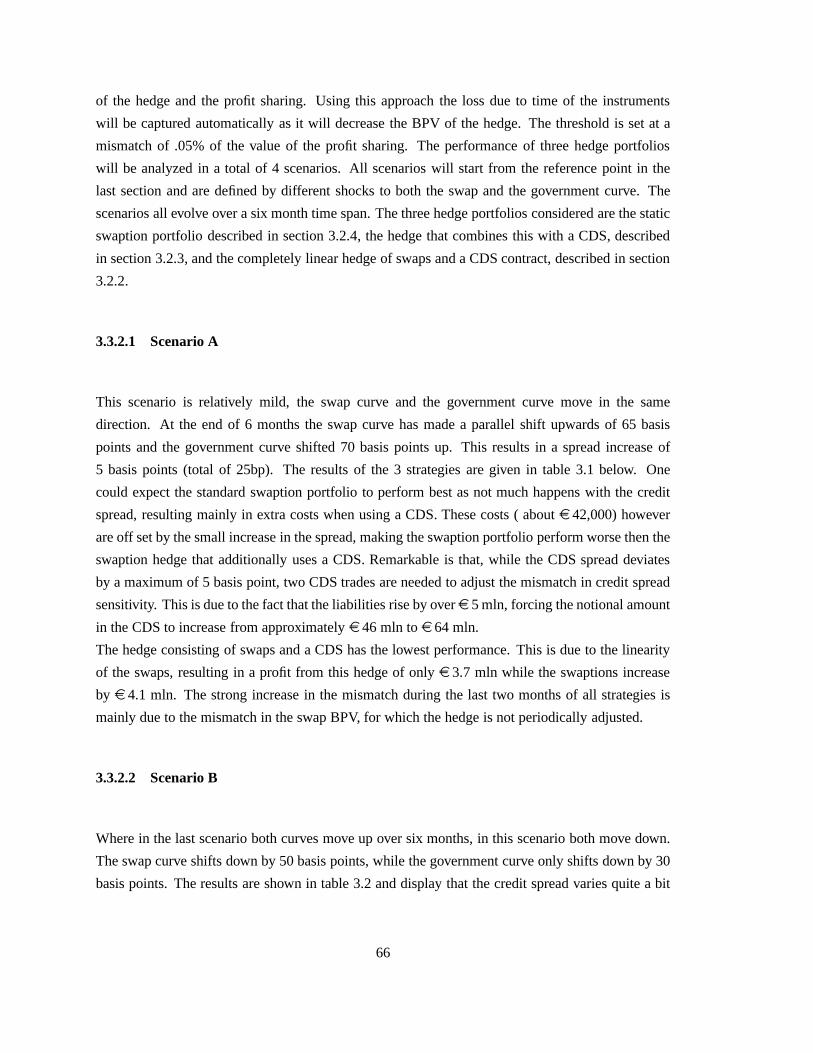
of the hedge and the profit sharing. Using this approach the loss due to time of the instruments

will be captured automatically as it will decrease the BPV ofthe hedge. The threshold is set at a

mismatch of .05% of the value of the profit sharing. The performance of three hedge portfolios

will be analyzed in a total of 4 scenarios. All scenarios willstart from the reference point in the

last section and are defined by different shocks to both the swap and the government curve. The

scenarios all evolve over a six month time span. The three hedge portfolios considered are the static

swaption portfolio described in section 3.2.4, the hedge that combines this with a CDS, described

in section 3.2.3, and the completely linear hedge of swaps and a CDS contract, described in section

3.2.2.

3.3.2.1 Scenario A

This scenario is relatively mild, the swap curve and the government curve move in the same

direction. At the end of 6 months the swap curve has made a parallel shift upwards of 65 basis

points and the government curve shifted 70 basis points up. This results in a spread increase of

5 basis points (total of 25bp). The results of the 3 strategies are given in table 3.1 below. One

could expect the standard swaption portfolio to perform best as not much happens with the credit

spread, resulting mainly in extra costs when using a CDS. These costs ( aboute 42,000) however

are off set by the small increase in the spread, making the swaption portfolio perform worse then the

swaption hedge that additionally uses a CDS. Remarkable is that, while the CDS spread deviates

by a maximum of 5 basis point, two CDS trades are needed to adjust the mismatch in credit spread

sensitivity. This is due to the fact that the liabilities rise by overe 5 mln, forcing the notional amount

in the CDS to increase from approximatelye 46 mln toe 64 mln.

The hedge consisting of swaps and a CDS has the lowest performance. This is due to the linearity

of the swaps, resulting in a profit from this hedge of onlye 3.7 mln while the swaptions increase

by e 4.1 mln. The strong increase in the mismatch during the last two months of all strategies is

mainly due to the mismatch in the swap BPV, for which the hedgeis not periodically adjusted.

3.3.2.2 Scenario B

Where in the last scenario both curves move up over six months, in this scenario both move down.

The swap curve shifts down by 50 basis points, while the government curve only shifts down by 30

basis points. The results are shown in table 3.2 and display that the credit spread varies quite a bit

66

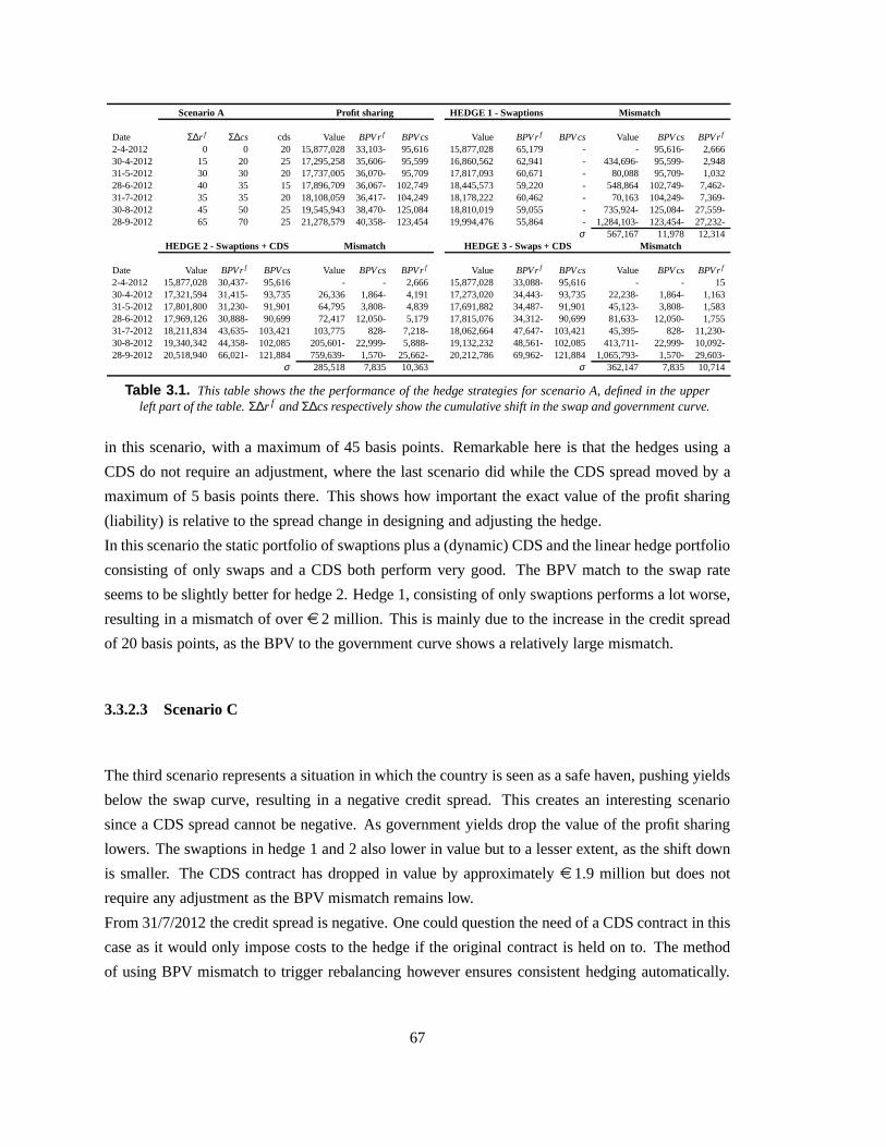
Scenario A Profit sharing HEDGE 1 - Swaptions Mismatch

Date Σ∆r f Σ∆cs cds Value BPVrf BPVcs Value BPVrf BPVcs Value BPVcs BPVrf

2-4-2012 0 0 20 15,877,028 33,103- 95,616 15,877,028 65,179 - - 95,616- 2,66630-4-2012 15 20 25 17,295,258 35,606- 95,599 16,860,562 62,941 - 434,696- 95,599- 2,94831-5-2012 30 30 20 17,737,005 36,070- 95,709 17,817,093 60,671 - 80,088 95,709- 1,03228-6-2012 40 35 15 17,896,709 36,067- 102,749 18,445,573 59,220 - 548,864 102,749- 7,462-31-7-2012 35 35 20 18,108,059 36,417- 104,249 18,178,222 60,462 - 70,163 104,249- 7,369-30-8-2012 45 50 25 19,545,943 38,470- 125,084 18,810,019 59,055 - 735,924- 125,084- 27,559-28-9-2012 65 70 25 21,278,579 40,358- 123,454 19,994,476 55,864 - 1,284,103- 123,454- 27,232-

σ 567,167 11,978 12,314HEDGE 2 - Swaptions + CDS Mismatch HEDGE 3 - Swaps + CDS Mismatch

Date Value BPVrf BPVcs Value BPVcs BPVrf Value BPVrf BPVcs Value BPVcs BPVrf

2-4-2012 15,877,028 30,437- 95,616 - - 2,666 15,877,028 33,088- 95,616 - - 1530-4-2012 17,321,594 31,415- 93,735 26,336 1,864- 4,191 17,273,020 34,443- 93,735 22,238- 1,864- 1,16331-5-2012 17,801,800 31,230- 91,901 64,795 3,808- 4,839 17,691,882 34,487- 91,901 45,123- 3,808- 1,58328-6-2012 17,969,126 30,888- 90,699 72,417 12,050- 5,179 17,815,076 34,312- 90,699 81,633- 12,050- 1,75531-7-2012 18,211,834 43,635- 103,421 103,775 828- 7,218- 18,062,664 47,647- 103,421 45,395- 828- 11,230-30-8-2012 19,340,342 44,358- 102,085 205,601- 22,999- 5,888- 19,132,232 48,561- 102,085 413,711- 22,999- 10,092-28-9-2012 20,518,940 66,021- 121,884 759,639- 1,570- 25,662- 20,212,786 69,962- 121,884 1,065,793- 1,570- 29,603-

σ 285,518 7,835 10,363 σ 362,147 7,835 10,714

Table 3.1. This table shows the the performance of the hedge strategiesfor scenario A, defined in the upperleft part of the table.Σ∆r f andΣ∆cs respectively show the cumulative shift in the swap and government curve.

in this scenario, with a maximum of 45 basis points. Remarkable here is that the hedges using a

CDS do not require an adjustment, where the last scenario didwhile the CDS spread moved by a

maximum of 5 basis points there. This shows how important theexact value of the profit sharing

(liability) is relative to the spread change in designing and adjusting the hedge.

In this scenario the static portfolio of swaptions plus a (dynamic) CDS and the linear hedge portfolio

consisting of only swaps and a CDS both perform very good. TheBPV match to the swap rate

seems to be slightly better for hedge 2. Hedge 1, consisting of only swaptions performs a lot worse,

resulting in a mismatch of overe 2 million. This is mainly due to the increase in the credit spread

of 20 basis points, as the BPV to the government curve shows a relatively large mismatch.

3.3.2.3 Scenario C

The third scenario represents a situation in which the country is seen as a safe haven, pushing yields

below the swap curve, resulting in a negative credit spread.This creates an interesting scenario

since a CDS spread cannot be negative. As government yields drop the value of the profit sharing

lowers. The swaptions in hedge 1 and 2 also lower in value but to a lesser extent, as the shift down

is smaller. The CDS contract has dropped in value by approximately e 1.9 million but does not

require any adjustment as the BPV mismatch remains low.

From 31/7/2012 the credit spread is negative. One could question the need of a CDS contract in this

case as it would only impose costs to the hedge if the originalcontract is held on to. The method

of using BPV mismatch to trigger rebalancing however ensures consistent hedging automatically.

67

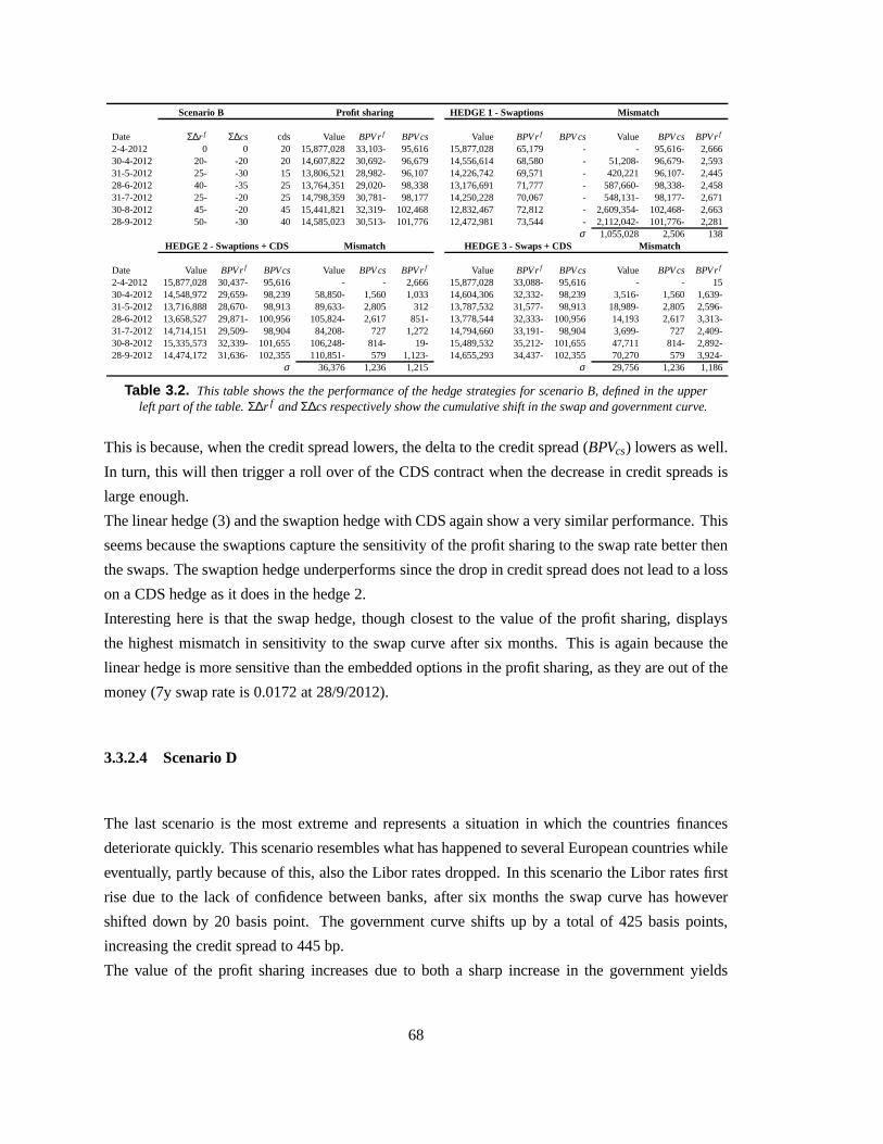
Scenario B Profit sharing HEDGE 1 - Swaptions Mismatch

Date Σ∆r f Σ∆cs cds Value BPVrf BPVcs Value BPVrf BPVcs Value BPVcs BPVrf

2-4-2012 0 0 20 15,877,028 33,103- 95,616 15,877,028 65,179 - - 95,616- 2,66630-4-2012 20- -20 20 14,607,822 30,692- 96,679 14,556,614 68,580 - 51,208- 96,679- 2,59331-5-2012 25- -30 15 13,806,521 28,982- 96,107 14,226,742 69,571 - 420,221 96,107- 2,44528-6-2012 40- -35 25 13,764,351 29,020- 98,338 13,176,691 71,777 - 587,660- 98,338- 2,45831-7-2012 25- -20 25 14,798,359 30,781- 98,177 14,250,228 70,067 - 548,131- 98,177- 2,67130-8-2012 45- -20 45 15,441,821 32,319- 102,468 12,832,46772,812 - 2,609,354- 102,468- 2,66328-9-2012 50- -30 40 14,585,023 30,513- 101,776 12,472,98173,544 - 2,112,042- 101,776- 2,281

σ 1,055,028 2,506 138HEDGE 2 - Swaptions + CDS Mismatch HEDGE 3 - Swaps + CDS Mismatch

Date Value BPVrf BPVcs Value BPVcs BPVrf Value BPVrf BPVcs Value BPVcs BPVrf

2-4-2012 15,877,028 30,437- 95,616 - - 2,666 15,877,028 33,088- 95,616 - - 1530-4-2012 14,548,972 29,659- 98,239 58,850- 1,560 1,033 14,604,306 32,332- 98,239 3,516- 1,560 1,639-31-5-2012 13,716,888 28,670- 98,913 89,633- 2,805 312 13,787,532 31,577- 98,913 18,989- 2,805 2,596-28-6-2012 13,658,527 29,871- 100,956 105,824- 2,617 851- 13,778,544 32,333- 100,956 14,193 2,617 3,313-31-7-2012 14,714,151 29,509- 98,904 84,208- 727 1,272 14,794,660 33,191- 98,904 3,699- 727 2,409-30-8-2012 15,335,573 32,339- 101,655 106,248- 814- 19- 15,489,532 35,212- 101,655 47,711 814- 2,892-28-9-2012 14,474,172 31,636- 102,355 110,851- 579 1,123- 14,655,293 34,437- 102,355 70,270 579 3,924-

σ 36,376 1,236 1,215 σ 29,756 1,236 1,186

Table 3.2. This table shows the the performance of the hedge strategiesfor scenario B, defined in the upperleft part of the table.Σ∆r f andΣ∆cs respectively show the cumulative shift in the swap and government curve.

This is because, when the credit spread lowers, the delta to the credit spread (BPVcs) lowers as well.

In turn, this will then trigger a roll over of the CDS contractwhen the decrease in credit spreads is

large enough.

The linear hedge (3) and the swaption hedge with CDS again show a very similar performance. This

seems because the swaptions capture the sensitivity of the profit sharing to the swap rate better then

the swaps. The swaption hedge underperforms since the drop in credit spread does not lead to a loss

on a CDS hedge as it does in the hedge 2.

Interesting here is that the swap hedge, though closest to the value of the profit sharing, displays

the highest mismatch in sensitivity to the swap curve after six months. This is again because the

linear hedge is more sensitive than the embedded options in the profit sharing, as they are out of the

money (7y swap rate is 0.0172 at 28/9/2012).

3.3.2.4 Scenario D

The last scenario is the most extreme and represents a situation in which the countries finances

deteriorate quickly. This scenario resembles what has happened to several European countries while

eventually, partly because of this, also the Libor rates dropped. In this scenario the Libor rates first

rise due to the lack of confidence between banks, after six months the swap curve has however

shifted down by 20 basis point. The government curve shifts up by a total of 425 basis points,

increasing the credit spread to 445 bp.

The value of the profit sharing increases due to both a sharp increase in the government yields

68

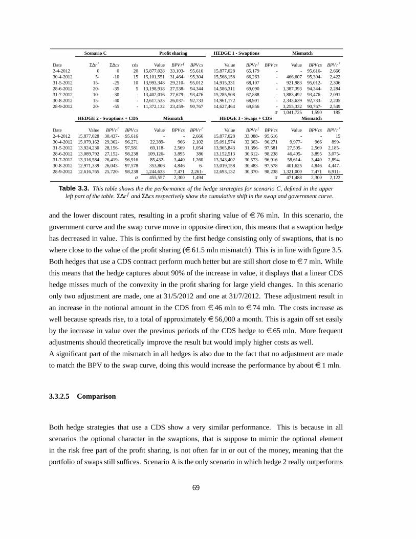
Scenario C Profit sharing HEDGE 1 - Swaptions Mismatch

Date Σ∆r f Σ∆cs cds Value BPVrf BPVcs Value BPVrf BPVcs Value BPVcs BPVrf

2-4-2012 0 0 20 15,877,028 33,103- 95,616 15,877,028 65,179 - - 95,616- 2,66630-4-2012 5- -10 15 15,101,551 31,464- 95,304 15,568,158 66,263 - 466,607 95,304- 2,42231-5-2012 15- -25 10 13,993,348 29,210- 95,012 14,915,331 68,107 - 921,983 95,012- 2,30628-6-2012 20- -35 5 13,198,918 27,538- 94,344 14,586,311 69,090 - 1,387,393 94,344- 2,28431-7-2012 10- -30 - 13,402,016 27,679- 93,476 15,285,508 67,888 - 1,883,492 93,476- 2,09130-8-2012 15- -40 - 12,617,533 26,037- 92,733 14,961,172 68,901 - 2,343,639 92,733- 2,20528-9-2012 20- -55 - 11,372,132 23,459- 90,767 14,627,464 69,856 - 3,255,332 90,767- 2,549

σ 1,041,725 1,590 185HEDGE 2 - Swaptions + CDS Mismatch HEDGE 3 - Swaps + CDS Mismatch

Date Value BPVrf BPVcs Value BPVcs BPVrf Value BPVrf BPVcs Value BPVcs BPVrf

2-4-2012 15,877,028 30,437- 95,616 - - 2,666 15,877,028 33,088- 95,616 - - 1530-4-2012 15,079,162 29,362- 96,271 22,389- 966 2,102 15,091,574 32,363- 96,271 9,977- 966 899-31-5-2012 13,924,230 28,156- 97,581 69,118- 2,569 1,054 13,965,843 31,396- 97,581 27,505- 2,569 2,185-28-6-2012 13,089,792 27,152- 98,238 109,126- 3,895 386 13,152,513 30,612- 98,238 46,405- 3,895 3,075-31-7-2012 13,316,584 26,419- 96,916 85,432- 3,440 1,260 13,343,402 30,573- 96,916 58,614- 3,440 2,894-30-8-2012 12,971,339 26,043- 97,578 353,806 4,846 6- 13,019,158 30,483- 97,578 401,625 4,846 4,447-28-9-2012 12,616,765 25,720- 98,238 1,244,633 7,471 2,261- 12,693,132 30,370- 98,238 1,321,000 7,471 6,911-

σ 455,557 2,300 1,494 σ 471,488 2,300 2,122

Table 3.3. This table shows the the performance of the hedge strategiesfor scenario C, defined in the upperleft part of the table.Σ∆r f andΣ∆cs respectively show the cumulative shift in the swap and government curve.

and the lower discount rates, resulting in a profit sharing value ofe 76 mln. In this scenario, the

government curve and the swap curve move in opposite direction, this means that a swaption hedge

has decreased in value. This is confirmed by the first hedge consisting only of swaptions, that is no

where close to the value of the profit sharing (e 61.5 mln mismatch). This is in line with figure 3.5.

Both hedges that use a CDS contract perform much better but are still short close toe 7 mln. While

this means that the hedge captures about 90% of the increase in value, it displays that a linear CDS

hedge misses much of the convexity in the profit sharing for large yield changes. In this scenario

only two adjustment are made, one at 31/5/2012 and one at 31/7/2012. These adjustment result in

an increase in the notional amount in the CDS frome 46 mln toe 74 mln. The costs increase as

well because spreads rise, to a total of approximatelye 56,000 a month. This is again off set easily

by the increase in value over the previous periods of the CDS hedge toe 65 mln. More frequent

adjustments should theoretically improve the result but would imply higher costs as well.

A significant part of the mismatch in all hedges is also due to the fact that no adjustment are made

to match the BPV to the swap curve, doing this would increase the performance by aboute 1 mln.

3.3.2.5 Comparison

Both hedge strategies that use a CDS show a very similar performance. This is because in all

scenarios the optional character in the swaptions, that is suppose to mimic the optional element

in the risk free part of the profit sharing, is not often far in or out of the money, meaning that the

portfolio of swaps still suffices. Scenario A is the only scenario in which hedge 2 really outperforms

69

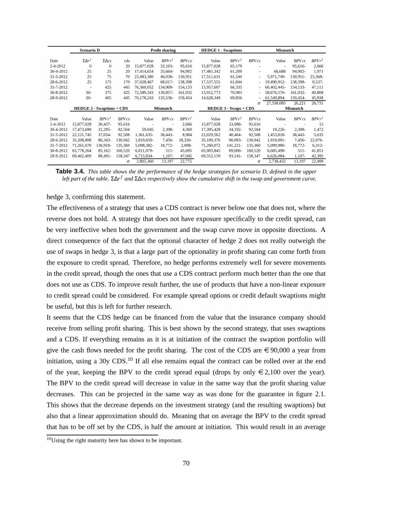
Scenario D Profit sharing HEDGE 1 - Swaptions Mismatch

Date Σ∆r f Σ∆cs cds Value BPVrf BPVcs Value BPVrf BPVcs Value BPVcs BPVrf

2-4-2012 0 0 20 15,877,028 33,103- 95,616 15,877,028 65,179 - - 95,616- 2,66630-4-2012 25 25 20 17,414,654 35,664- 94,902 17,481,342 61,209 - 66,688 94,902- 1,97131-5-2012 25 75 70 23,483,380 46,038- 130,951 17,511,631 61,544 - 5,971,749- 130,951- 23,368-28-6-2012 25 175 170 37,028,467 68,017- 138,398 17,537,55561,844 - 19,490,912- 138,398- 8,537-31-7-2012 - 425 445 76,360,052 134,909- 154,133 15,957,60766,335 - 60,402,445- 154,133- 47,11130-8-2012 30- 375 425 72,589,343 130,857- 161,032 13,912,773 70,983 - 58,676,570- 161,032- 40,80828-9-2012 20- 405 445 76,178,243 135,536- 159,454 14,628,349 69,856 - 61,549,894- 159,454- 45,938

σ 27,338,085 26,221 26,731HEDGE 2 - Swaptions + CDS Mismatch HEDGE 3 - Swaps + CDS Mismatch

Date Value BPVrf BPVcs Value BPVcs BPVrf Value BPVrf BPVcs Value BPVcs BPVrf

2-4-2012 15,877,028 30,437- 95,616 - - 2,666 15,877,028 33,088- 95,616 - - 1530-4-2012 17,473,699 31,295- 92,504 59,045 2,398- 4,369 17,395,428 34,192- 92,504 19,226- 2,398- 1,47231-5-2012 22,121,745 37,054- 92,508 1,361,635- 38,443- 8,984 22,029,562 40,404- 92,508 1,453,818- 38,443- 5,63528-6-2012 35,208,808 86,343- 130,942 1,819,659- 7,456- 18,326- 35,109,376 90,093- 130,942 1,919,091- 7,456- 22,076-31-7-2012 71,261,670 136,918- 135,360 5,098,382- 18,772-2,008- 71,260,072 141,221- 135,360 5,099,980- 18,772- 6,312-30-8-2012 65,778,264 85,162- 160,520 6,811,079- 511- 45,695 65,903,845 89,006- 160,520 6,685,498- 511- 41,85128-9-2012 69,462,409 88,491- 158,347 6,715,834- 1,107- 47,045 69,552,159 93,141- 158,347 6,626,084- 1,107- 42,395

σ 2,805,360 13,197 22,775 σ 2,738,432 13,197 22,499

Table 3.4. This table shows the the performance of the hedge strategiesfor scenario D, defined in the upperleft part of the table.Σ∆r f andΣ∆cs respectively show the cumulative shift in the swap and government curve.

hedge 3, confirming this statement.

The effectiveness of a strategy that uses a CDS contract is never below one that does not, where the

reverse does not hold. A strategy that does not have exposurespecifically to the credit spread, can

be very ineffective when both the government and the swap curve move in opposite directions. A

direct consequence of the fact that the optional character of hedge 2 does not really outweigh the

use of swaps in hedge 3, is that a large part of the optionalityin profit sharing can come forth from

the exposure to credit spread. Therefore, no hedge performsextremely well for severe movements

in the credit spread, though the ones that use a CDS contract perform much better than the one that

does not use as CDS. To improve result further, the use of products that have a non-linear exposure

to credit spread could be considered. For example spread options or credit default swaptions might

be useful, but this is left for further research.

It seems that the CDS hedge can be financed from the value that the insurance company should

receive from selling profit sharing. This is best shown by thesecond strategy, that uses swaptions

and a CDS. If everything remains as it is at initiation of the contract the swaption portfolio will

give the cash flows needed for the profit sharing. The cost of the CDS aree 90,000 a year from

initiation, using a 30y CDS.10 If all else remains equal the contract can be rolled over at the end

of the year, keeping the BPV to the credit spread equal (dropsby only e 2,100 over the year).

The BPV to the credit spread will decrease in value in the sameway that the profit sharing value

decreases. This can be projected in the same way as was done for the guarantee in figure 2.1.

This shows that the decrease depends on the investment strategy (and the resulting swaptions) but

also that a linear approximation should do. Meaning that on average the BPV to the credit spread

that has to be off set by the CDS, is half the amount at initiation. This would result in an average

10Using the right maturity here has shown to be important.

70

notional ofe 23 mln, equaling total cost ofe 1.4 mln over 30 years. The cost of the CDS is thus

less than the amount received as premium, what seems plausible as the CDS is not a perfect match.

One should then be able to buy the optional character with what is left.

If the situation does change, and profit sharing increases, this is due to the fact that the government

yields have increased. If the credit spreads have remained equal, the cash flows from the swaptions

should still match the ones needed for profit sharing, as the swap rates have increased. If the swap

curve has remained the same, the increase is due to a larger credit spread. This value is captured

by the CDS hedge. Rolling over the CDS will now result in larger costs due to the increased CDS

spread. These cost can be financed by the increase in the hedgeportfolios value.

3.4 A practical implementation

In this section the performance of the hedge strategies is analyzed using historical data on the CDS

spread and government yields of Spain over the period 31/3/2005 - 1/4/2012. In the computation of

these results the assumption is not made that the CDS spread is equal to the credit spread. 5 year

CDS spreads are used to compute the values of 30 year contracts. This is done because quotes on

30 year Spanish CDS contracts are limited as a result of the fact that Spain generally issues debt

with low maturities. Normally the term structure is slightly upward sloping, so this might result in

costs that are estimated a bit to low. The Libor hedges, both by swaps and by swaptions, are again

static. The CDS contract is rolled over based on similar criteria as discussed in the last section, only

the monitoring is done quarterly. Finally, because the government curve is modeled from actual

historical data, the shifts do not have to be parallel as theywere in the last section. All results are

displayed in figure 3.6.

The figure immediately reveals that the two portfolios that do not consider exposure to the

government curve explicitly (Swaps(Old) and Swaptions) perform significantly worse than the two

strategies that do. The hedge that uses swaptions instead ofswaps together with the CDS contracts,

performs very well up till 30/6/2010, while over this periodthe CDS spread has risen 240 basis

points. The spikes that follow are due to large jumps in the CDS spread, not exactly coinciding with

the jumps in credit spread (see also figure 3.1). This shows animportant property of CDS spreads,

as they can be very volatile compared to bond spreads.

The portfolio that uses swaps does not seem to track the profitsharing as well but does result in the

best performance at the end of the period. This mostly due to the fact that the CDS spreads moves

stronger than the bond spreads do over this period. But as well because of the fact that the swap

71

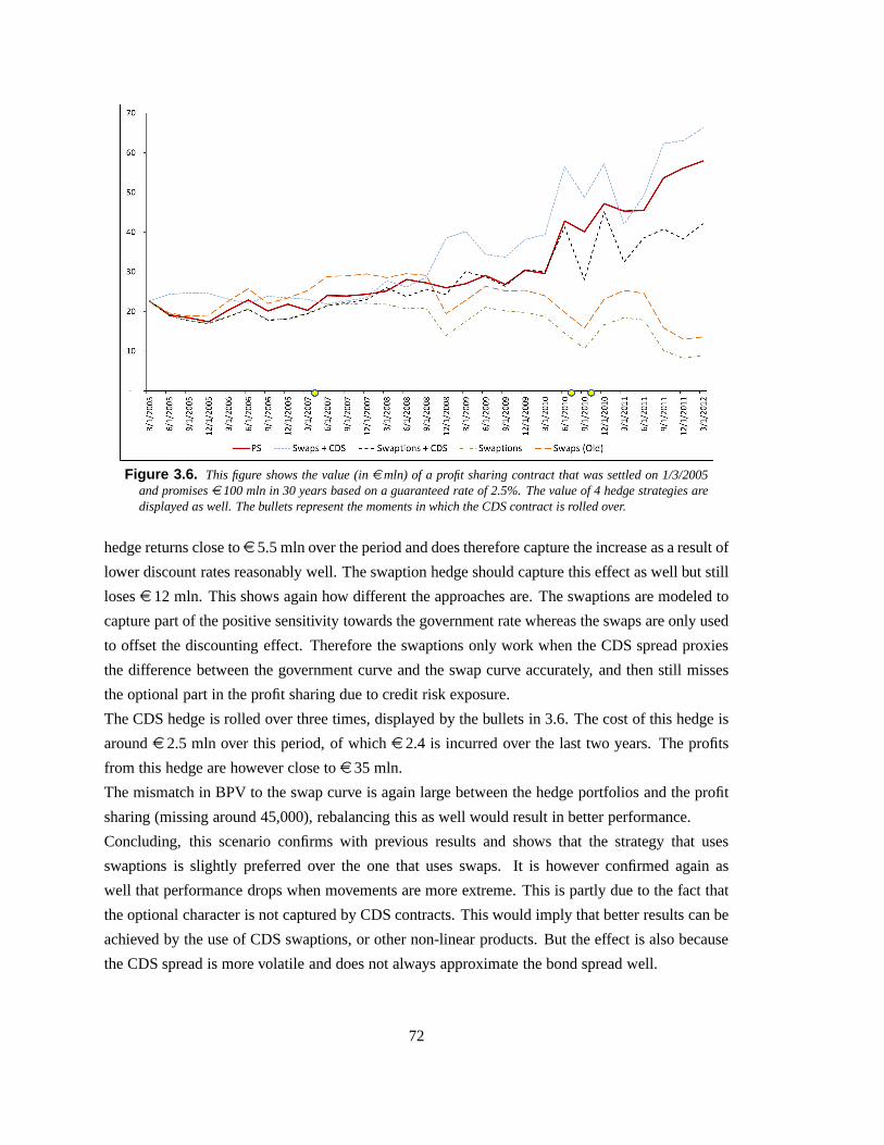
Figure 3.6. This figure shows the value (inemln) of a profit sharing contract that was settled on 1/3/2005and promisese 100 mln in 30 years based on a guaranteed rate of 2.5%. The value of 4 hedge strategies aredisplayed as well. The bullets represent the moments in which the CDS contract is rolled over.

hedge returns close toe 5.5 mln over the period and does therefore capture the increase as a result of

lower discount rates reasonably well. The swaption hedge should capture this effect as well but still

losese 12 mln. This shows again how different the approaches are. The swaptions are modeled to

capture part of the positive sensitivity towards the government rate whereas the swaps are only used

to offset the discounting effect. Therefore the swaptions only work when the CDS spread proxies

the difference between the government curve and the swap curve accurately, and then still misses

the optional part in the profit sharing due to credit risk exposure.

The CDS hedge is rolled over three times, displayed by the bullets in 3.6. The cost of this hedge is

arounde 2.5 mln over this period, of whiche 2.4 is incurred over the last two years. The profits

from this hedge are however close toe 35 mln.

The mismatch in BPV to the swap curve is again large between the hedge portfolios and the profit

sharing (missing around 45,000), rebalancing this as well would result in better performance.

Concluding, this scenario confirms with previous results and shows that the strategy that uses

swaptions is slightly preferred over the one that uses swaps. It is however confirmed again as

well that performance drops when movements are more extreme. This is partly due to the fact that

the optional character is not captured by CDS contracts. This would imply that better results can be

achieved by the use of CDS swaptions, or other non-linear products. But the effect is also because

the CDS spread is more volatile and does not always approximate the bond spread well.

72

3.5 Summary

This chapter started with a short overview on what has been done in the field of risk management at

insurance companies. Several hedge strategies were discussed, following in a way the approach of

Coleman et al. (2003), by local optimization (match BPV’s) and the use of a zero coupon bond to

equal the final value.

In the construction of the hedge strategies special attention has gone to the exposure to credit spread,

of which the importance was discussed in the previous chapter. For this, the use of a CDS contract

was considered elaborately, including several effects that could influence the effectiveness of the

hedge but were not analyzed here.

In the evaluation of the strategies, the hedges that use a CDShave shown to be a significant

improvement to the ones that do not. The one that uses swaptions and a CDS should match the

profit sharing better, but this is only visible when swap rates increase substantially. A large part of

the value of the profit sharing can result from the non-linearexposure towards the credit spread. If

movements are not to extreme, the CDS contract seems to be able to capture the effect reasonably

well.

In chapter 2 it was already suggested that the value of the profit sharing is probably to large to finance

from the difference between the premium received by the insurer and the cost of the guarantee.

Because the cost of the contract should equal the price in themarket in the end and the CDS

hedge proposed here does not replicate the value of the profitsharing exactly, results imply that

this mismatch pointed out in chapter 2 might even be larger.

73

Conclusion

This work started off with a comprehensive discussion of a profit sharing product that is typically

sold by Dutch insurance companies. The motivation for the existence of this product is twofold;

1) it provides a level of security to the policyholder through a guaranteed return and keeps upside

potential when interest rates are high 2) for the insurance company its value lies in the stability

of the profit sharing and in that it allows the insurance company to market a product that is

competitive. The product differs from many profit sharing products in other countries with respect

to the underlying factor that determines the return. This isbecause profit sharing is based on a

fixed income investment portfolio that invests in fictitiousbonds. The yield of these bonds, called

the u-yield, is determined by the yields on Dutch governmentbonds via a complicated weighting

scheme.

In chapter 1, methods were discussed to construct replicating portfolios that are consistent with the

value of the product. These portfolios were build of swaptions in combination with a zero coupon

bond. Also a hands on approach was provided to quickly estimate the value of such a product

when the investment policy gets more complicated. This camedown to finding an optimal trade off

between matching the weight of investments and the timing ofprofit sharing. These methods should

prove useful in preparations for Solvency II, which requires market based accounting and will force

insurance companies to estimate the value of the embedded options in this product accurately.

Due to the complicated structure of the u-yield and to simplify computations, most calculations

involving these products are currently based on the seven year swap rate. This is because these rates

have shown to behave very similar historically. In the second chapter it is however reasoned that

these rates are fundamentally different and that it can be dangerous to assume a constant spread

between the two. The implications of doing this were assessed using an alternative model to

value the replication portfolios. This model estimates thevalue of the profit sharing product while

acknowledging sensitivity to both the risk free rate and thecountries credit spread. Results show that

not considering the credit spread can lead to substantial errors in valuation and consequently also

in the design of risk mitigating strategies. Furthermore, the model can provide additional insight in

74

the dynamics of the profit sharing products sensitivities, which is important in the construction and

performance appraisal of hedge strategies.

This chapter has also shown that the value of the guarantee islikely to add significant pressure

on the capital buffers of many insurance companies today. Itwas observed that the shape of the

government curve is of large influence to the value of the profit sharing product through the forward

rates used to value the swaptions. This confirms once more theimportance of explicitly considering

two curves in the valuation of these products. It was shown that the credit spread has a strong

positive effect on the value of the profit sharing.

The last chapter has pointed out important differences between unit-linked contracts and profit

sharing contracts. The most relevant difference is that credit risk in profit sharing contracts is to

be held by the insurance company, where it is held by the policyholder in unit-linked contracts.

The exposure to credit risk should be taken into consideration when designing risk mitigating

strategies. The importance of doing this, and the implications of not doing this, were analyzed

using various hedge strategies in scenarios with varying discount curves and credit spreads. Both the

instantaneous performance and the effectiveness over a larger time span were assessed. The hedge

strategies considered are constructed by matching the sensitivity to several parts of the applicable

curve in basis point value (BPV). Both non-linear hedges consisting of swaptions and linear hedges

consisting of swaps were evaluated. The effectiveness of including CDS contracts in hedging credit

risk was assessed as well. Results show that the performanceof the strategies that use swaps instead

of swaptions are very similar. Only when swap rates increasesignificantly a portfolio of swaptions

is preferred. The use of a CDS contract in mitigating exposure to credit risk seems very effective

when a roll over strategy based on BPV mismatch is applied. Only when the credit spread increases

dramatically the linear payoff from the CDS contract does not completely capture the optional

character that the spread displays in the profit sharing. Ideally, multiple CDS contracts should be

used to exactly match exposure to credit risk on different parts of the curve. The most important

parts are determined by the fictive investment policy and contract maturity. CDS contracts with

long maturities can be used to minimize costs, as these allowfor a lower fee. This method seems to

result in an effective hedge, despite the mismatch in exposure. Hedge strategies constructed while

not considering exposure to credit risk perform well for scenarios in which the government and

swap curve move in an equal direction simultaneously. However, they severely under perform when

this is not the case.

Results of chapter 1 and 2 already suggested that the profit sharing could not be financed from the

difference between the amount that the insurers receive as apremium from the policy holder and

the cost of the guarantee in the market. The fact that the bestperforming hedge strategies in chapter

3 are still not perfect, again raise the question what the fair value of such a contract should be. The

results all point in the direction that these contracts are being sold below their market value. This

75

might however still be equal to the fair value of this contract to the consumer, as he or she might not

expect to receive payments with a 100% probability.

Although this work has discussed many aspects of the profit sharing product in great detail, it still

allows for enough improvements and contributions to be made. The model can be extended by

developing a way to incorporate the volatility matrix of theforward curve11 in the valuation of the

replicating portfolio, instead of using the volatility of the discount curve. Furthermore significant

contributions could be added by considering more instruments to hedge the credit risk in these

products. But also by assessing effectiveness in a more complete way, i.e., considering the side

effects that were discussed in paragraph 3.2.2.1. Interesting would also be to consider different

measures in constructing a hedge portfolio. Here, this was done by minimizing the mismatch in

BPV’s, meaning that risk is minimized locally. One could also use linear or dynamic programming

to minimize risk over a larger quadrant, i.e., constructingthe hedge based on minimization of the

mismatch over multiple curve shifts. Here, also non-parallel curve shifts could be considered.

Finally, in this thesis it was assumed that the contractual promise made to the policyholder is very

strict. Often however, there is a clause in such a contract that states the insurance company can

keep itself from paying the profit sharing under certain circumstances. This is not considered here

because it is outside the cope of this thesis and the likelihood of an insurer doing this is estimated

to be small. It would significantly damage the credibility ofthe insurance company and the trust of

the consumer in the product. The clause however still represents some kind of counter option that

would be interesting to consider in the valuation.

In summary, this work has discussed the profit sharing product elaborately and provided the reader

with insights into the factors that influence the value and into the risks that these products introduce.

Important here was the exposure to country credit risk, thatwas assessed using a model that

considers sensitivity towards two interest rate curves. Results showed that the use of a portfolio

consisting of swaptions and a CDS contract can be expected toprovide a robust hedge for the

profit sharing element. Furthermore, the discussion of the risks and the hedge strategies, the

insights provided by the model and the suggestions given above should provide a fruitful ground

for further research. A useful recommendation to insurers could be to modify the contract slightly,

by promising profit sharing based on the swap rate instead of the u-rate, or to model exposure to

credit risk explicitly. Neglecting this exposure in risk management can lead to severe errors in the

valuation and in the design of an effective hedge.

11The applicable government curve.

76

References

Black, F. and Scholes, M. (1973). The pricing of options and corporate liabilities. Journal of

Political Economy 81.

Bouwknegt, P. and Pelsser, A. (2001). Marktwaarde van winstdeling. De Actuaris.

Boyle, P. and Schwartz, E. (1997). Equilibrium prices of guarantees under equity linked contracts.

Journal of Risk and Insurance 44.

Briys, E. and de Varenne, F. (1994). Life insurance in a contingent claim framework : pricing and

regulatory implications.The Geneva Papers on Risk and Insurance Theory.

Coleman, T., Li, Y., and Patron, M. (2003). Discrete hedgingunder piecewise linear risk

minimization. Journal of Risk, nr. 5.

Dieckmann, S. and Plank, T. (2010). Default risk of advancedeconomies: An emperical analysis of

credit default swaps during the financial crises.

DNB (2012). Overzicht financiële stabiliteit voorjaar 2012. Overzicht Financiële Stabiliteit, nr. 15.

Donselaar, J. (1999). Guaranteed returns: risks assured.Nederlands Auctuarieel genootschap.

Duffie, D. (1999). Credit swap valuation.Financial Analysts’ Journal, nr. 83.

Dutch State Treasury Agency (2011). Outlook 2012.Outlook.

Ejsing, J. and Lemke, W. (2010). The janus-headed salvation: Sovereign and bank credit risk premia

during 2008-09.ECB Working paper 1127.

Föllmer, H. and Sondermann, D. (1986). Hedging of non redundant contingent claims.

Contributions to mathematical economics. Hildebrand, W. ,Mas-Colell,A.

Fontana, A. and Scheicher, M. (2010). An analysis of euro area sovereign cds and their relation

with government bonds.Working Paper No. 1271.

77

Grosen, A. and Jorgensen, P. (2000). Fair valuation of life insurance liabilities: The impact of

interest rate guarantees, surrender options, and bonus policies. Insurance: Mathematics and

Economics.

Hipp, C. (1996). Aktienindexgebundene lebensversicherung mit garantierter verzinsung.Z. Vers.

Wiss.

Hull, J. (2008).Option, Futures, and other Derivatives.Pearson.

Macaulay, F. (1910). Money, credit and the price of securities. Insurance: Mathematics and

Economics, nr. 48.

Miltersen, K. and Persson, S. (2000). Guaranteed investment contracts: distributed and

undistributed excess return.Working Paper, Institute of Finance and Management Science.

Moller, T. (2001). Risk-minimizing hedging strategies forinsurance payment processes.Finance

and stochastics, Nr. 5.

Nteukam, T., Planchet, F., and Thérond, P. (2011). Optimal strategies for hedging portfolios of

unit-linked life insurance contracts with minimum death guarantee.Insurance: Mathematics and

Economics, nr. 48.

Pelsser, A. (2008). Pricing and hedging guaranteed annuityoptions via static option replication.

Insurance: Mathematics and Economics 33.

Plat, R. (2005). Analystische waardering van opties op u-rendement.De Auctuaris.

Plat, R. and Pelsser, A. (2008). Analytical approximationsfor prices of swap rate dependent

embedded options in insurance products.Insurance: Mathematics and Economics 44.

Schrager, D. and Pelsser, A. (2006). Pricing swaptions and coupon bond options in affine term

structure models.Mathematical Finance 16.

Sibbett, T. (1996). Life office bonuses; the road to 90-10.The Actuary.

78

Appendix A

A.1 Function descriptions

A.1.1 Profit sharing function

This appendix provides information about the tool that is used in this thesis to simulate expected

cash flows originating from profit sharing products. Becausethe theory behind these products is

discussed in chapter 1 the focus here will be more on tool specific subjects as input, output and

calculations that are not trivial.

The main purpose of the tool is to make projections about profit sharing based on some interest

rate scenario and product specifications and to construct a replicating portfolio that mimics the

profit sharing payments that are expected. Before computations are discussed first a note on the

installation will be given and all the input parameters thatare used need to be defined.

Installation instructions.

The tool can be accessed by installing the Excel Add-In in which the code of the function resides.

The best way to do this is to put the Add-In in the Microsoft AddIns folder with the default address:

"C:/Documents and Settings/<user>/Application Data/Microsoft/AddIns". Then install the AddIn

in Excel by going to:

File→ Options→ Add-Ins→ Go.., and selecting "Winstdeling Functie".

79

A.1.1.1 Input and parameters

The tool can be used as a function in Excel after the Add-In hasbeen installed under the function

name "Overrente". This function requires 8 parameters and has 5 additional optional parameters:

Curve. This is the most important parameter, it represents the interest rate term structure on which

all calculations are based and needs to be passed as a Curve object as it is computed by the

CardanoLib.

Template. This provides information about what output has to be printed. Possible values, that

mostly have a trivial meaning but will also be explained in the text below, are:

"All, FV Premium, FV Reserve, FV Investments, FV PL, 7ySwaprate, URate, Uw, FV Profit

Share, FV Swaption Cashflows, FV Swaptions, PV Swaptions, DF, Notionals, NRPD"

Expected cash flows.This parameter needs to be entered as an by 2 array, wheren is the number

of cash flows. In the first column the date of the cash flows, in the second the amount that has

to be paid to policyholders. Or it can be entered as an by 1 array with only the cash flows. In

this case theperiodlengthhas to be entered as optional parameter as well.

Guaranteed rate. This is the rate that is guaranteed to the policyholders annually no matter what

the return on investments has been.

Fee. This parameter represents the fee the insurer can charge by subtracting a percentage from the

profit share. If there is no profit sharing in a year no fee is paid, if there is, first the fee is paid

and the remainder goes to the policyholder.

Maturity. This parameter represents the maturity of the investments that are made in the investment

portfolio.

Type. This specifies what should be done with possible profit sharing. Values can be either 1)

"Payout", meaning that the amount is paid out to the policyholder or 2) "Reinvest", meaning

that the amount is added to the reserve and invested.

Distribute premiums. This parameter specifies whether all expected cash flows are presented as

one lump sum payment at inception or that premiums are equalized for all cash flows and

distributed to according periods.

Turnover. This parameter is optional. By default it is set to 1, meaningthat the notionals of the

investments are paid back in full at maturity. If another payment structure is preferred it

should be entered as amby 1 array, wherem is the maturity of the investments that are made

in the fictive portfolio. The elements in the array should sumto 1.

Model. This is an optional parameter that gives the user the abilityto specify what should be

modeled; either "Profit Sharing" or "Guarantee".

80

DiscountCurve. This parameter is optional. If the user wants to value the product using two curves,

the discount curve should be entered here. The forward curveshould be entered as first

variable.

Period length. This is an optional parameter that should be entered if the expected cash flows are

entered as ann by 1 array. Values should be in the tenor "im" or "iy", for respectively months

or years.i must be an integer.

FixedVol. This is an optional parameter that gives the user the abilityto use a fixed value for the

volatility instead of using the entire volatility matrix from the function library that belongs to

the start date of the curve.

The function can then be used by of selecting a range, based onthe preferred output (template), and

following the standard procedure of entering array formulas in Excel with

"=Overrente(Curve, Template, ExpectedCashFlows, rg, Fee, Maturity, Type, DistributePremiums)"

A.1.1.2 Calculations

The calculations start with the evaluation of the expected cash flows to the policy holders.

Depending on the parameterDistribute premiums{False,True} the cash flows are discounted to:

1. False : One big lump sum payment at origin:

Pj =

n∑

i=0df iCFi if j = 0,

0 if j 6= 0,

with df i the discount factor of periodi at inception based on the guaranteed raterg that is

provided to the function andCFi the cash flow belonging to this date.

2. True : All cash flows are distributed to fixed premiums in a way that the sum of all premiums,

including the interest, exactly matches the expected cash flow at the period the cash flow has

to be paid to the policyholders. The sum of all the premiums ina period contributing to the

cash flows expected from that period onward then represents the total amount received by the

insurer.

81

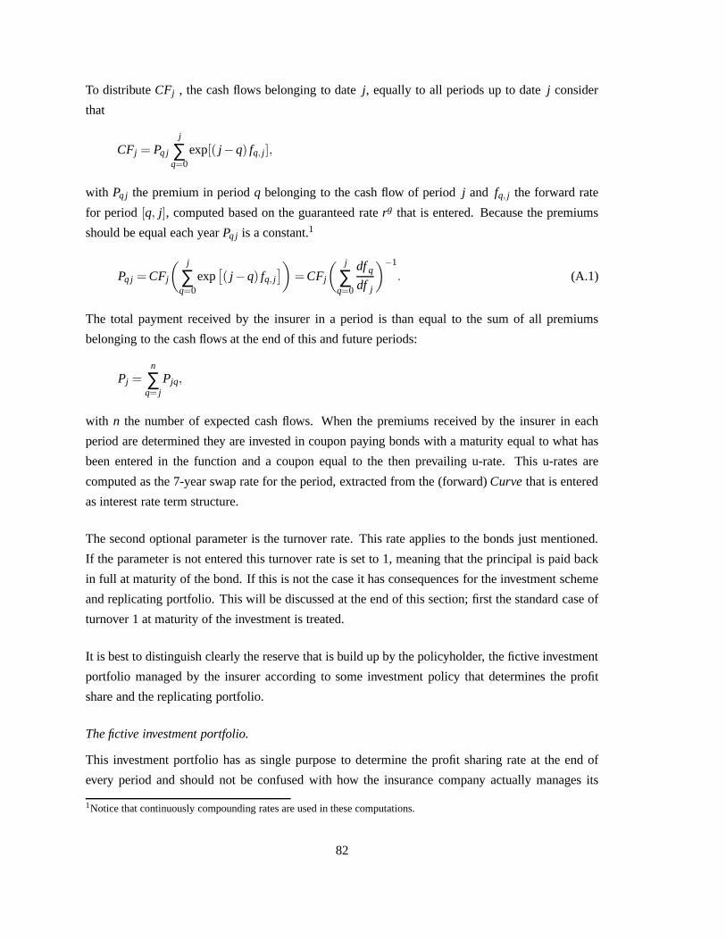
To distributeCFj , the cash flows belonging to datej, equally to all periods up to datej consider

that

CFj = Pq j

j

∑q=0

exp[( j −q) fq, j ],

with Pq j the premium in periodq belonging to the cash flow of periodj and fq, j the forward rate

for period [q, j], computed based on the guaranteed raterg that is entered. Because the premiums

should be equal each yearPq j is a constant.1

Pq j =CFj

( j

∑q=0

exp[

( j −q) fq, j]

)

=CFj

( j

∑q=0

dfq

df j

)−1

. (A.1)

The total payment received by the insurer in a period is than equal to the sum of all premiums

belonging to the cash flows at the end of this and future periods:

Pj =n

∑q= j

Pjq,

with n the number of expected cash flows. When the premiums receivedby the insurer in each

period are determined they are invested in coupon paying bonds with a maturity equal to what has

been entered in the function and a coupon equal to the then prevailing u-rate. This u-rates are

computed as the 7-year swap rate for the period, extracted from the (forward)Curvethat is entered

as interest rate term structure.

The second optional parameter is the turnover rate. This rate applies to the bonds just mentioned.

If the parameter is not entered this turnover rate is set to 1,meaning that the principal is paid back

in full at maturity of the bond. If this is not the case it has consequences for the investment scheme

and replicating portfolio. This will be discussed at the endof this section; first the standard case of

turnover 1 at maturity of the investment is treated.

It is best to distinguish clearly the reserve that is build upby the policyholder, the fictive investment

portfolio managed by the insurer according to some investment policy that determines the profit

share and the replicating portfolio.

The fictive investment portfolio.

This investment portfolio has as single purpose to determine the profit sharing rate at the end of

every period and should not be confused with how the insurance company actually manages its

1Notice that continuously compounding rates are used in these computations.

82

assets. This fictive portfolio is usually defined by a simple investment policy that invests in one

type of fixed income asset with a fixed maturity ofM years and a certain turnover structure for the

principal payments. The policy is described in more detailsbelow.

For each periodi the premiums and the payments and coupons of the previous investments are

received. Depending on theTypealso the profit share over the last period is added to this sum and

the total amount is then invested in bonds (the fixed income asset) yielding the then prevailing

u-rateui .

At the end of each period a weighted u-rate can be determined by computing the return on the fictive

investment portfolior f ii . This weighted u-rate then determines the profit share over the last periodi :

r f ii =

i

∑q=(i−M+1)+

ruqIqIΣ,i

, IΣ,i =i

∑q=(i−M+1)+

Iq,

(i −M+1)+ = max(i −M+1,0),

with M the maturity,Iq the amount invested in periodq, often called a layer, andIΣ,i the sum of all

investments in previous layers. The profit sharingPSi is then

PSi = Ri max[

r f ii − (rg+δ ),0

]

,

whereRi is the amount in the reserve at the beginning of periodi andδ is the fee entered in the

function. The amount that has to be paid to the policyholdersat the end of the period is then the profit

sharing and the cash flow based on the contracts entered as array in the function. The amount of

the cash flows has to be subtracted from the investment portfolio by reducing the notionals invested

against the u-rates by a factor1−CFiIΣ,i

, resulting in coupons and payments reduced by the same factor.2

The reserve.

This portfolio tracks what rights the policy holders have build up and what, at the end of the

contracts, has to be paid out. In the case the profit share is paid out every period this is the sum

of the premiums and the accrued interest. In the case that theprofit share is reinvested two things

need to be considered:

- The extra interest over the profit share.

- Future profit share over the amount received as profit share now. This means the policyholder

will receive options on profit sharing in future dates, complicating the product.

2This suggest assets are liquidated equally over all layers in the fictive investment portfolio to cover the liabilities.

83

The reserve is linked to the investment portfolio through the initial amount in the investment

portfolio that equals the premiums paid at inception by the policy holders. IfPSi is positive and

the profit share will be paid out to the policyholder, the investment portfolio will decrease by the

same amount. If the profit share is reinvested the reserveRi increases withPSi .

If the return on the fictive portfolior f ii is lower than the guaranteed rate there will be no profit

share. Because the reserve enjoys a minimum return equal to the guaranteed rate the amounts in

both portfolios will diverge. The loss that is made by the insurer is tracked by a loss account that

has Template valueFV PL. The interest on the loss account is determined at the end of each period

and equals the swap rate with appropriate maturity extracted from the discount object entered into

the function.

In the case 0≤ r f ii − rg ≤ δ the amount in the investment portfolio increases with a rateexceeding

the reserves byr f ii − rg.

The replicating portfolio.

This is the portfolio that replicates the profit sharing partof the product, not the entire portfolio.3

The profit sharing part of the product resembles the positionin a strip of payer swaptions by the

policyholder on the weighted u-rate rater f ii as this cannot be modeled by one swaption because the

option of a positive profit share is each period and the notional amount changes each period. As

mentioned in the text it is not possible, or to expensive, to buy swaptions on the u-rate, let alone a

weighted u-rate, and therefore the swaptions are based on the 7-year swap rate assuming that this is

a good proxy for the u-rate (see section 1.3). The use of a weighted u-rate causes it to look more

like an Asian option on a 1 year swap, but then not using just anaverage but a weighing scheme

proportional to the investments made up toq periods back by the investment portfolio, whereq is

equal to the maturity of the investments. A strip ofM year swaptions is used to model the weighing,

with M the maturity of underlying investments.

The way the swaption portfolio is the build up is by buying a swaption on theM year swap rate

with an expiration date that equals the beginning of each period, a maturity equal to the maturity of

the investments, a notional proportional to the amount thatis invested that period and a strike equal

to rg+ δ .4 This means that at the end of every period there will be possible payoffs of a number

of swaps and these payoffs will have a weighing to the total payoff equal to the weights that the

u-rates have in the computation of the fictive investment portfolio returnr f ii . Because the sum of the

investments in the fictive portfolio does not have to match the reserve and the profit sharing is paid

out over the reserve the notionals are not exactly equal to the investments of the fictive portfolio.

3If this is required the calculation can be done easily by summing with the values of zero coupon bonds with similarmaturity and principal as the cash flows resulting from the contracts.

4If the maturity differs from 7 years a adjustment should be made to the strike. This is explained in section 1.6.

84

The correct way to model this is to use notionals following the guaranteed rate, but that are based on

the investment policy of the fictive portfolio.5 This way the correct size and weighing is combined.6

One thing that should be mentioned is that, by modeling it in this way, there might be multiple

payoffs from the replicating portfolio every period but there is only paid one possible profit sharing,

based onr f ii . In other words, it will never be the case that there is no payoff from the replicating

portfolio when there is a profit sharing. This reflects that this replication is quite dominant and not

exact.

The above can be shown in a similar recursive way as before:

At the beginning of periodi the swaption needed has a notional of

Ni =i

∑q=(i−M+1)+

rgqIg

q + Igi−M +1{Type}PSi ,

with 1{Type} an indicator function returning 1 if Type is "Reinvest" and the superscriptg means that

the investments are based on the guaranteed raterg instead of the u-yieldui .

The swaption needed at inception then has the properties:

1. Notional Ni

2. Expiration date Datei

3. Strike rg

4. Maturity Maturity of investments.

5. Volatility Implied volatility of 7 year swap rate.

6. Tenors 1 year.

At the end of each period one swaption expires and a maximum ofM cash flows are received from

the swaps underlying previously expired swaptions that were in the money. The swap payoffs,

showed byFV Swaption Cashflows, are

CFswaps,i =i

∑q=(i−M+1)+

Nqmax[

uq− (rg+δ ),0]

.

5In case the profit share is reinvested this amount should be added.6A more extensive explanation is given in section 1.5.

85

These are the cash flows that should replicate the profit shareat yeari:

Ri max[

r f ii − (rg+δ ),0

]

≈i

∑q=(i−M+1)+

Nqmax[

uq− (rg+δ ),0]

.

The replicating portfolio is linked to the reserve by the useof the guaranteed raterg in determining

the notionals and simultaneously to the investment portfolio through the use of the same turnover

structure and maturity of the fictive investments.

From the above it should be clear that the required swaptionsare first determined based on the

guaranteed raterg and the policy of the investment portfolio. Based on theCurveobject the present

value of the swaptions at each period can be calculated by useof the expected forward curve in a

period. This is dislayed byPV Swaptionsof which the value at the beginning of periodi is:

PVi(Swaptions) =n

∑q=i

Swaptionq(

FCurvei ,Notionalq,Σu, rg+δ ,q,M

)

],

with FCurveq the forward curve in periodi andM the maturity of the swap that equals the maturity

of the investments.

If a specific turnover structure is used in the investment portfolio this has two important

consequences for the investment policy and replicating portfolio.

The consequences for the investments policy are that at eachperiod the payments of all previous

investments up to the maturity of the investments have to be taken into account. The principals of

the underlying investments that are made against the different u-rates then decline which in turn

make that the coupons will vary over time.

This turnover structure has consequences for the replicating portfolio as well. The notionals

change in the first place because of the amount available for investments in a period includes more

payments. The declining value of the principles also decline and therefore the weight the different

u-rates have in determiningr f ii will change, making it less sensitive to investments further back.

To be able to exactly match this, one would need a swaption with a declining notional. Another

approach would be, though swap rates make it slightly different, to use a number of swaptions per

investment layer. For example, if the principal of a bond with a maturity of 5 years is paid back

in 5 periods by equal amounts (15), this can be modeled by using 5 swaptions: one with a notional

of 15 of the investment and a maturity of 5 years, one with a notional of 1

5 of the investment and a

maturity of 4 years, etc..7 Because for the tool a general approach is needed, the problem is tackled

7See section 1.6 for more information on replicating strategies for different turnover structures.

86

by changing the maturity of the underlying swap to be the weighted maturity of the investments

based on the turnover structure.

Mw =M−1

∑i=0

(M− i)τΣ,i , τΣ,i =i+1

∑q=1

τq,

whereτq is the turnover in theqth year of the investments.

Section 1.6 shows that this is however not always the best wayto replicate the profit sharing and that

this should be tested on a case by case basis, the code in the tool can be adjusted relatively easily to

speed up this process.

A.1.2 Hedge evaluation function

This section describes the function that quickly analyzes the value and the BPV of a hedge strategy.

It is part of the AddIn that also contains the "Profit sharing function".

A.1.2.1 Input and parameters

The tool can be used as a function in Excel under the name "EvaluateHedge". It can be used to

evaluate hedge portfolios consisting of swaps, swaptions or CDS contracts.8 The function requires

3 parameters and has one additional optional parameter:

Date. This is the date on which the portfolio is bought.

Instruments. This parameter is entered as a range. The size of the range depends on the type of

instruments:Swap swaption,endtenor, rate, notional

Swaption swap,starttenor, endtenor, strike, p/r, notional

CDS CDS,starttenor, endtenor, CDS spread, notionalCurve. The curve is used to value the instruments. It is entered as a curve object computed by the

CardanoLib.

Evaluation Arguments. This is an optional argument. Here the CDS spread and default

probabilities can be entered.

8It can be extended to include other instruments in a simple way.

87

A.1.2.2 Calculations

The swaps and swaptions are valued by use of the Cardano Function Library. The value of the CDS

in computed as was described in section 3.2.2.1. The BPV is calculated by the difference in value

when the curve shifts up by one basis point. This shift is parallel and does therefore not compute

sensitivities to all different parts of the curve.

The output is given in a 1 by 2 array. In the first cell the value of the hedge portfolio, in the second

cell its BPV for a parallel shift.

A.2 Financial products

This section contains a brief overview of the financial products that are used in this thesis. Only

a very short description of the purpose of the product and itsvaluation will be given. For a more

detailed treatment see Hull (2008), sections 13.8, 7.7 and 28.3 respectively.

A.2.1 Option

In finance an option gives the holder the right, but not the obligation, to buy or sell something. This

something is called the underlying and can be anything from astock to a container of pork bellies.

A call option is defined as the option to buy the underlying on afuture date for a predetermined

price (the strike price), the right to sell a put option. The term European specifies that the option

can only be exercised at this future date (the expiration date). If it would be the case that the option

can be exercised at any time up to the expiration date it wouldbe an American option. Under some

assumptions Black and Scholes (1973) found an analytic expression for the value of an European

call option, from which the value of the put option can be deduced.

C = SN (d1)−K exp−rTN (d2), (A.2)

with,

d1 =logS/K +(r +σ2)T

σ√

T, d2 = d1−σ

√T.

88

In this formulaS represents the value of the underlying,K the strike price,r the risk free interest

rate,σ the standard deviation of the underlying,T time to the expiration date,N the cumulative

standard normal distribution function.

A.2.2 Swap

A swap represents an exchange of cash flows between two entities. The most well known, and also

the one used in this thesis, is the interest rate swap. In thisswap one entity agrees to pay a floating

interest rate (Libor9 + spread) to receive a fixed rate. At inception the value of a swap is usually

zero because the swap rate sets the value of the fixed leg exactly equal to the value of the floating

leg. At a later point in time the swap will have a value different from zero as Libor will vary over

time. The easiest way to value a swap is to see it as the difference between two bonds:

S= Bf ix −Bf l ,

whereBf ix is a fixed bond with coupons set by the swap rate,Bf l a floating rate bond paying Libor

+ spread and both bonds having the same notional and maturity.

A.2.3 Swaption

A swaption is a combination of the two financial products described above. The underlying in the

option,S in equation A.2, is simply the value of the swap. The expiration date of the swaption, in

the way it is used in this thesis, is the start date of the swap.

A.3 Terminology

At of the money If the value of the underlying is currently equal to the strike price of an option

the option is said to be at the money.

Discount rate The value ofe 1 today (the present value) is greater thane 1 next year. The

discount rate is used to translate future values to the present values and it is closely related to the

9London inter bank offered rate

89

discount factor.

Duration Duration is a mathematical expression introduced by Macaulay (1910) that captures

the weighted average term to maturity of a fixed income product by considering all cash flows

associated with the product.

Implied volatility The implied volatility of an option contract is the volatility that, based on a pricing

model, yields a value for the option equal to the current market price of that option.

In the money If the value of the underlying is currently above (below) thestrike price of an option

the option is said to be in the money for a call (put) option.

Modified duration The modified duration is a linear approximation for the percentage change in

value of a fixed income product when the yield changes by one unit and is closely related to the

duration and BPV.

Notional A financial contract is always based on some underlying asset. For fixed income

product, e.g. bonds and swaps, this is just some amount of cash over which the interest is paid

or yield is computed. This amount is called the notional amount, or, mainly for bonds, the principal

amount.

Option In finance an option is a derivative contract, it derives its value from some underlying

asset. The variety in options is enormous but in general there are two types of options: 1) acall

option and 2) aput option. They respectively give the right, but not the obligation, to buy and sell

the underlying for a predetermined price (strike price) during (American option) or at (European

option) expiration of the option.

Out of the money If the value of the underlying is currently above (below) thestrike price of an

option the option is said to be out of the money for a put (call)option.

Solvency II Solvency II reviews the capital adequacy and risk management standards for the

European insurance industry and will replace Solvency I. The main difference with Solvency I will

be the extensive use of market based valuation practices.

Strike This is the predetermined price used in the valuation of an option. (See option).

Swap A swap represents an exchange of cash flows between two entities. The most well known,

and also the one used in this thesis, is the interest rate swap. In this swap one entity agrees to pay

90

a floating interest rate (Libor + spread) to receive a fixed rate. At inception the value of a swap is

usually zero because the swap rate sets the value of the fixed leg exactly equal to the value of the

floating leg. At a later point in time the swap will have a valuedifferent from zero as Libor will vary

over time.

Swap rate The swap rate is the fixed rate that sets a swap contracts market value at initiation to

zero. (See also swap)

Swaption This product gives the holder the the right, but not the obligation, to buy a underlying

swap for a predetermined price. The underlying swaps are interest rate swaps. There are two kinds

of swaptions; 1) apayer swaption and 2)receiver swaption. Respectively for an underlying swap

that pays a fixed rate and one that receives a fixed rate over thenotional.

Unit- and equity linked products These are two type of insurance plans of which the

value changes based on an existing underlying reference portfolio of assets. Unit-linked

contracts generally allow investments in a combination of both equity and and debt instruments.

Equity-linked products only allow investments in equities. It is often easier to withdraw funds

from equity-linked saving plans and the cost charges are lower. Most equity-linked contracts do not

have an insurance element in them, whereas unit-linked contracts usually do.

91