riikka peltokangas and aki sorsa - university of...
TRANSCRIPT

CONTROL ENGINEERING LABORATORY
Real-coded genetic algorithms and nonlinear parameter identification
Riikka Peltokangas and Aki Sorsa
Report A No 34, April 2008

University of Oulu Control Engineering Laboratory Report A No 34, April 2008
Real-coded genetic algorithms and nonlinear parameter identification
Riikka Peltokangas and Aki Sorsa
University of Oulu, Control Engineering Laboratory Abstract: Macroscopic models are useful for example in process control and optimization. They are based on the mass balances describing the flow conditions and the assumed reaction scheme. The development of a process model typically has two steps: model structure selection and parameter identification. The structure selection step is not discussed in this report. In the parameter identification step, the squared error criterion is typically minimized. It can be done with conventional methods such as gradient methods but genetic algorithms is used in this study instead. That is because genetic algorithms are very likely to find the global minimum as the conventional methods may stuck in local minimums. Real-coded genetic algorithms are used in this study. Thus the first part of this report reviews the crossover and mutation operators used for regulating the development of population. A process simulator of a bioprocess is used to generate data for parameter identification. The bioprocess model is known to be nonlinear having two separate operating points. Thus the process model is identified in two operating conditions. The mean squared error criterion is used to determine the validity of possible solutions to optimization problem. Parameter identification with genetic algorithms performed well giving good results. The optimizations are repeated 500 times to guarantee the validity of the results. The results are further validated by examining the mean and the standard deviation of the prediction error as well as the mean squared error criterion. Also correlation coefficients are calculated and the histograms of the parameter values in all 500 optimizations are studied. Keywords: macroscopic bioprocess model, parameter identification, genetic algorithms ISBN 978-951-42-8786-2 (pdf) University of Oulu ISSN 1238-9390 Control Engineering Laboratory P.O. Box 4300 FIN-90014 University of Oulu

TABLE OF CONTENTS 1 INTRODUCTION ...................................................................................................... 1 2 GENETIC ALGORITHMS ........................................................................................ 2 3 CROSSOVER OPERATORS IN REAL-CODED GENETIC ALGORITHMS........ 4
3.1 Arithmetic crossover method (AMXO) ............................................................... 4 3.2 Heuristic crossover operator ............................................................................... 4 3.3 Parent-centric crossover operators ...................................................................... 5 3.4 Laplace crossover operator ................................................................................. 5 3.5 The BLX-α crossover operator ............................................................................ 7 3.6 The PBX-α crossover operator ............................................................................ 7 3.7 Multiple crossover .............................................................................................. 8 3.8 Linear crossover.................................................................................................. 9 3.9 Extended line crossover ...................................................................................... 9 3.10 Fuzzy Connectives Based Crossover (FCB)....................................................... 9 3.11 Direction-based crossover (DBXO) .................................................................. 11 3.12 Hybrid crossover methods ................................................................................ 11 3.13 Crossover in a real-coding jumping gene genetic algorithm ............................ 12
4 MUTATION OPERATORS IN REAL-CODED GENETIC ALGORITHMS........ 14 4.1 Makinen, Periaux and Toivanen Mutation........................................................ 14 4.2 Non-Uniform Mutation (NUM)........................................................................ 15 4.3 Power Mutation (PM) ....................................................................................... 16 4.4 Uniform Mutation ............................................................................................. 17 4.5 Boundary Mutation ........................................................................................... 17 4.6 Mutation in RJGGA.......................................................................................... 17
5 PARAMETER IDENTIFICATION OF A BIOPROCESS MODEL....................... 19 5.1 Generated data sets ........................................................................................... 19 5.2 Applied genetic algorithms ............................................................................... 20 5.3 Identification of the model parameters for the first operating point ................. 21 5.4 Identification of the model parameters for the second operation point ............ 24
6 CONCLUSIONS AND DISCUSSION .................................................................... 26 REFERENCES ................................................................................................................. 27

1
1 INTRODUCTION
Macroscopic models of processes are useful in many ways. They can be used for example in process optimization and control. Such models consist of a set of mass balances for macroscopic species. The mass balances describe the phenomena occurring in the reactor. In chemical and biochemical applications, macroscopic models are based on the assumed reaction scheme and the flow conditions. The development of an accurate model needs some a priori knowledge especially in selecting a valid reaction scheme and kinetic model structure. If no process knowledge is available, black-box modelling tools must be used. (Grosfils et al. 2007) Modelling typically involves model structure selection and parameter identification steps. Model structure selection is not discussed in this report because the model structure is known. The parameter identification procedure typically minimizes the squared error criterion. Conventional optimization methods (such as gradient methods) can be used in identification. However, the outcome of these methods depends on the initial guess because optimization may be stuck at local minimums instead of finding the global one. Such problems do not exist if genetic algorithms are used in parameter identification. Genetic algorithms basically cover the whole search space and search the optimal solutions from multiple directions due to the genetic operations (crossover and mutation) regulating the optimization. Thus genetic algorithms are more likely to find the optimal (or at least near-optimal) solution. (Chang 2007) In this study, genetic algorithms are used to identify process parameters. The results from similar research can be found from literature, for example from Chang (2007). A process simulator is used to generate data sets for the identification. The simulator is based on the model of a continuous bioreactor with Haldane kinetics. The process shows bistable behaviour leading to a two-peaked distribution of the output variables (Sorsa and Leiviskä 2006). The model parameters are identified in two distinct operating points. This study also discusses the methods for validating the results obtained with genetic algorithms. This report is organized as follows. First, genetic algorithms are introduced followed by a literature review about the crossover and mutation methods used in genetic algorithms. The rest of the report presents the obtained results.

2
2 GENETIC ALGORITHMS
Genetic algorithms (GA) are optimization methods mimicking evolution. Optimization is based on the development of the population comprising a certain number of chromosomes. The development of the population is regulated in two ways: crossover and mutation. The evolution of population is illustrated in figure 1. A possible solution to the optimization problem is coded to each chromosome. Binary or real valued coding can be used. If binary coding is used, each variable must be represented by a suitable number of bits to guarantee an accurate enough solution (Davis 1991). The link between the population and the optimization problem is the objective function. It is used to evaluate the suitability of different solutions and thus the goodness of each chromosome.
Crossing andmutation
The best solution fromthe last population
Value of the objective function
Initial population New populationCrossing andmutation
The best solution fromthe last population
Value of the objective function
Initial populationInitial population New populationNew population
Figure 1. The evolution of population in genetic algorithms. In crossover, new chromosomes are generated from the old ones. Usually steady-state crossover is used, where two chromosomes (parents) are fused to generate two new chromosomes (offspring). The parents are selected randomly so that better chromosomes have higher probability to be selected as parents. Thus the population evolves to better solutions. (Davis 1991) The tournament and the roulette wheel methods are typically used in parent selection. In tournament selection method a certain number of chromosomes are selected randomly to participate in a “tournament”. The chromosome with the highest (lowest) goodness value is the winner and is selected as a parent. In the roulette wheelselection method, the cumulative sum of the goodness values is calculated. A random number is then generated between the minimum and the maximum of the cumulative sum. The point where the random number intercepts the cumulative sum curve determines the parent. The roulette wheel selection is illustrated in figure 2.

3
510152025303540455055
1 2 3 4 5 6 7 8 9 10
Chromosome
Cum
ulat
ive
sum Random number
510152025303540455055
1 2 3 4 5 6 7 8 9 10
Chromosome
Cum
ulat
ive
sum Random number
Figure 2. The roulette wheel selection method. Random changes are generated to the population in mutation. This prevents the population from converging towards a local optimum. Elitism can also be used with genetic algorithms. In elitism, a fraction of the best chromosomes from the previous population is placed to the new population. Thus, the best chromosomes never disappear from the population through crossover or mutation. (Davis 1991)

4
3 CROSSOVER OPERATORS IN REAL-CODED GENETIC ALGORITHMS
After parents have been selected by the selection method, crossover takes place. Crossover operator mates the parents to produce offspring. Crossover consists of swapping chromosome parts between individuals but is not performed on every pair of individuals. The crossover frequency is controlled by a crossover probability (pc). (Arumugam et al. 2005) Typically, parents are denoted as:
)x,...,x(x
)x,...,x(x)(
n)()(
)(n
)()(
221
2
111
1
=
= (1)
Similar representation is also used for offspring:
)y,...,y(y
)y,...,y(y)(
n)()(
)(n
)()(
221
2
111
1
=
= (2)
Above, x(i) is the i:th parent, y(j) is the j:th offspring and n is the number of crossovers per generation. Equations 1 and 2 are both written for the case of two parents and offspring. Depending on the applied crossover operator the number of parents and offspring may vary. Following is a short review of used crossover methods.
3.1 Arithmetic crossover method (AMXO)
In arithmetic crossover, two parents produce two offspring. Thus the parents are as defined by equation 1. The offspring are arithmetically the following (Kaelo and Ali 2007):
,)1(
,)1()1()2()2(
)2()1()1(
iiiii
iiiii
xxy
xxy
αα
αα
−+=
−+= (3)
where iα are uniform random numbers (Michalewicz 1998). Furthermore, α is constant in uniform arithmetical crossover or it may vary with regard to the number of generations made in non-uniform arithmetical crossover (Herrera et al., 1998).
3.2 Heuristic crossover operator
Heuristic crossover (HX) has been applied to solve nonlinear constrained optimization problems (Michalewicz 1995). More experiments with HX are reported in (Michalewicz

5
et al, 1996). HX is also applied on constrained as well as unconstrained optimization problems having various levels of difficulty. (Deep and Thakur 2007a) In HX, two parents are mated. Thus the parents are as defined by equation 1. Unlike other crossover operators HX produces at most one offspring from a given pair of parents and it makes use of fitness function values of parents in producing offspring. The offspring is generated in the following manner (Deep and Thakur 2007a):
)2()1()2( )( iiii xxxy +−=α (4) Above, α is a uniformly distributed random number in the interval [0, 1]. It should be noticed that the parent )2(x has fitness value not worse than that of the
parent )1(x . If the offspring lies outside the feasible region, a new random number is generated to produce another offspring using (Deep and Thakur 2007a):
)2()1()2()2(iiii xxxy −+= β (5)
Above, β is a random number, which is generated using the Laplace distribution function. This process is repeated up to k times. In Deep and Thakur (2007a), the performance of this crossover was tested with a set of 20 test problems available in the global optimization literature.
3.3 Parent-centric crossover operators
Parent-centric crossover operators (PCCO) create the offspring in the neighborhood of the female parent using a probability distribution. The male parent is considered to define the range of the probability distribution. (García-Martínez et al. 2008) PCCOs are a meaningful and efficient way of solving real-parameter optimization problems. In García-Martínez et al. (2008), PCCOs are considered to work like self-adaptive mutation operators and that is the reason why they are suitable for the design of effective local search procedures. More information about PCCOs is presented in García-Martínez et al. (2008).
3.4 Laplace crossover operator
In Deep and Thakur (2007a), a new crossover operator which uses Laplace distribution was introduced. This parent-centric crossover operator has been named as Laplace Crossover (LX) operator. The density function of Laplace distribution is the following:

6
,exp21)( ⎟⎟
⎠
⎞⎜⎜⎝
⎛ −−=
bax
bxf ∞<<∞− x (6)
The corresponding distribution function is as follows:
⎪⎪
⎩
⎪⎪
⎨
⎧
>⎟⎟⎠
⎞⎜⎜⎝
⎛ −−−
≤⎟⎟⎠
⎞⎜⎜⎝
⎛ −
=
ax,b
axexp
ax,b
axexp
)x(F
211
21
(7)
Above, Ra∈ is the location parameter and b > 0 is the scale parameter. Figure 3 shows the density function when a = 0 for both b = 0.5 and b = 1.
Figure 3. Density function of Laplace distribution (a = 0, b = 0.5 and b = 1) (Deep and Thakur 2007a). Two offspring are generated from a pair of parents in the following way (Deep and Thakur 2007a): A uniformly distributed random number α ∈[0, 1] is generated. A random number β is generated which follows the Laplace distribution by simply inverting the distribution function of Laplace distribution (equation 7) as follows:
⎪⎪⎩
⎪⎪⎨
⎧
>+
≤−=
21),ln(
21),ln(
αα
ααβ
ba
ba (8)

7
The offspring are given by the equations (Deep and Thakur 2007a):
)(i
)(i
)(i
)(i
)(i
)(i
)(i
)(i
xxxy
xxxy2122
2111
−+=
−+=
β
β (9)
Both offspring are placed symmetrically with respect to the position of the parents. For smaller values of b, offspring are likely to be produced near the parents. For larger values of b, offspring are expected to be produced far from the parents. If the parents, for fixed values of a and b, are near to each other the offspring are expected to be near to each other. Otherwise they are likely to be far from each other. This way the proposed crossover operator has self adaptive behavior. The performance of this crossover was also tested with a set of 20 test problems available in the global optimization literature. The comparative study showed that LX performed quite well and LX with Makinen, Periaux and Toivanen mutation outperformed the other used GAs in Deep and Thakur (2007a).
3.5 The BLX-α crossover operator
The BLX-α crossover operator mates two parents to produce one offspring. An offspring is the following:
),...,,...,( 1 ni yyyy = (10) where iy is a randomly (uniformly) chosen number of the interval [li - Iα ui+ Iα]. The terms for equation 10 are calculated by:
⎪⎪⎩
⎪⎪⎨
⎧
−==
=
ii
)(i
)(ii
)(i
)(ii
luI)x,xmin(l
)x,xmax(u21
21
(11)
3.6 The PBX-α crossover operator
In Garcia-Martinez et al. (2008) a parent-centric BLX-α crossover operator (PBX-α) is used. In PBX-α two parents produce one offspring. The offspring is given by equation 10. The difference compared to BLX-α is that yi is a randomly (uniformly) chosen number from the [li, ui] interval. The limits li and ui are given by:
⎪⎪⎩
⎪⎪⎨
⎧
−=
+=
−=
)(i
)(i
)(iii
)(iii
xxI
}Ix,bmax{u
}Ix,amax{l
21
2
1
α
α
(12)

8
Above, )1(x is called the female parent, and )2(x the male parent. The effects of the crossover are presented in figure 4. The female parents point to search areas that will receive sampling points. The male parents determine the extent of these areas. α is used to determine the spread associated with the probability distributions used to create offspring.
Figure 4. Effects of the PBX-α operator. (García-Martínez et al. 2008) In García-Martínez et al. (2008), minimization experiments on six problems were carried out. They included three unimodal functions, two multimodal functions and one complex real-world problem.
3.7 Multiple crossover
In Chang (2006) and Chang (2007), a multi-crossover formula with more than two chromosomes was proposed. It was assumed that three chromosomes )1(x , )2(x and
)3(x are selected from the population randomly and crossed by one another. In Chang (2006), a search space for IIR filter coefficients (θ ) was the following:
},...,,|Rx{ maxmmminmmaxminminM
x θθθθθθθ ≤≤≤≤∈=Ω 2221 (13) All genes ,iθ for mi∈ , in a chromosome were evolved in the search space xΩ during genetic operations. If any values in the produced chromosome goes beyond xΩ , then the original chromosome was retained. It was assumed that α is a random number selected from [0, 1]. If cp≥α , no crossover operation is performed. If cp<α , then the multiple crossover formulas are the following:
) x-x x(rxx
) x-x x(rxx
) x-x x(rxx
)()()()()(
)()()()()(
)()()()()(
32133
32122
32111
2
2
2
−+=′
−+=′
−+=′
(14)
Above, ]1,0[∈r is a random value determining the crossover grade.

9
In Chang (2006), an improved real-coded GA was proposed to accurately identify IIR digital filter coefficients. All unknown filter coefficients were collected as a chromosome, and a population of these chromosomes was evolved using genetic operations. The multiple crossover provided a better adjusting vector on chromosomes to generate more excellent offspring. The effectiveness of the proposed multiple crossover was verified by simulating the band pass and band stop IIR filters. In Chang (2007), a multi-crossover was used to determine PID controller gains for multivariable processes. The defined performance criterion of integrated absolute error (IAE) was minimized. A multivariable binary distillation column process with strong interactions between input and output pairs, and different time delays, was used to demonstrate the effectiveness of the proposed method. Compared to the traditional crossover operators, better output responses and minimal IAE values were obtained from simulation results.
3.8 Linear crossover
In linear crossover, two parents produce two offspring. However, three offspring are generated initially. The offspring are defined by:
)(i
)(i
)(i
)(i
)(i
)(i
)(i
)(i
)(i
xxy
xxy
xxy
213
212
211
23
21
21
23
21
21
+−=
−=
+=
(15)
An offspring selection mechanism is applied, which chooses the two most promising offspring of the three to substitute their parents in the population.
3.9 Extended line crossover
In extended line crossover, one offspring is generated from two parents. The offspring is given by (Mühlenbein and Schlierkamp-Voosen 1993, Popovic and Murty 1997):
)( )1()2()1(iiii xxxy −+= α (16)
Above, α is randomly (uniformly) chosen value in the interval [-0.25, 1.25].
3.10 Fuzzy Connectives Based Crossover (FCB)
The interval of action of the gene i ],[ ii ba may be divided into three regions as shown in figure 5. The intervals described could be classified as exploration or exploitation zones.

10
The interval with both genes being the extremes is an exploitation zone and the two intervals that remain on both sides are exploration zones. The region with extremes /
iα and /iβ could be considered as a relaxed exploitation zone. (Herrera et al. 1998)
Figure 5. Action interval for a gene (Herrera et al. 1998). In Herrera et al. (1997) four functions F, S, M and L are defined from ],[],[ baba × in
],,[ ba ,, Rba ∈ and they fulfill: (P1) ],[, baxx ∈′∀ },,min{),( xxxxF ′≤′ (P2) ],[, baxx ∈′∀ },,max{),( xxxxS ′≥′ (P3) ],[, baxx ∈′∀ },,max{),(},min{ xxxxMxx ′≤′≤′ (P4) ],[, baxx ∈′∀ ),,(),(),( xxSxxLxxF ′≤′≤′ (P5) F, S, M, and L are monotone and non-decreasing. The offspring is generated by:
),,( )2()1(iii xxQy = n,...,i 1= (17)
T-norms, t-conorms, averaging functions and generalized compensation operators may be used to obtain F, S, M and L operators. In Herrera et al. (1998) F is associated to a t-norm T, S to a t-conorm G, M with an averaging operator P, and L with a generalized compensation operator C . A set of linear transformations are needed to be able to apply these operators under the gene definition intervals. A set of functions F, S, M and L are built, which are the following:
),(ˆ)(),(
),()(),(),()(),(),()(),(
ssCabaxxL
ssPabaxxMssGabaxxSssTabaxxF
′⋅−+=′
′⋅−+=′′⋅−+=′′⋅−+=′
(18)
Above, abaxs
−−
= and abaxs
−−′
=′ .

11
These operators have the property of being continuous non-decreasing functions. Applications of these operators to the population are presented in Herrera et al. (1997). The operators establish an exploration or exploitation relationship by selecting the most suitable offspring. Required diversity levels in the population are therefore increased.
3.11 Direction-based crossover (DBXO)
Problem-specific knowledge is introduced into genetic operators in order to produce improved offspring. Direction-based crossover uses the values of the objective function in determining the direction of genetic search. The operator generates single offspring y from two parents )1(x and )2(x according to the following: (Arumugam et al. 2005)
)2()1()2( )( xxxy +−=α (19) where α is a random number between 0 and 1. It is assumed that the parent )2(x is not worse than )1(x :
)x(f)x(f )()( 12 ≤ (20) In Lu and Tzeng (2000), a direction-based crossover was used to deal with the design of arbitrary FIR log filters.
3.12 Hybrid crossover methods
In Arumugam and Rao (2004), four hybrid crossover methods were designed from AMXO (Arithmetical crossover) and ACXO (Average Convex crossover). In Lee and Mohamed (2002), a hybrid crossover method was applied to control system design of a power plant. The used hybrid crossover was applied to simultaneously find gains of three PI control loops and six other coupled gains in a Boiler-Turbine control system. The method had a better convergence rate when applied to this problem, as compared to other methods. A comparison between hybrid crossover and convex crossover in RCGA together with multipoint crossover using binary coded GA was also made. In Figure 6, a hybrid real-coded genetic algorithm with local search is presented.
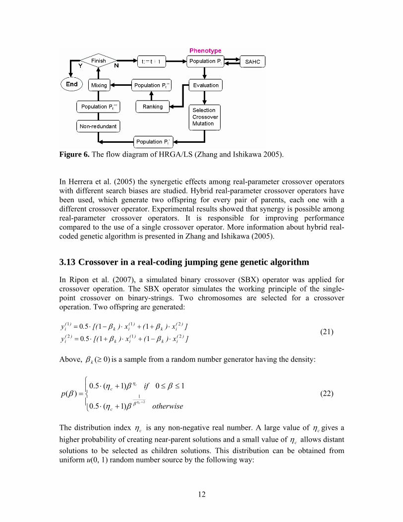
12
Figure 6. The flow diagram of HRGA/LS (Zhang and Ishikawa 2005). In Herrera et al. (2005) the synergetic effects among real-parameter crossover operators with different search biases are studied. Hybrid real-parameter crossover operators have been used, which generate two offspring for every pair of parents, each one with a different crossover operator. Experimental results showed that synergy is possible among real-parameter crossover operators. It is responsible for improving performance compared to the use of a single crossover operator. More information about hybrid real-coded genetic algorithm is presented in Zhang and Ishikawa (2005).
3.13 Crossover in a real-coding jumping gene genetic algorithm
In Ripon et al. (2007), a simulated binary crossover (SBX) operator was applied for crossover operation. The SBX operator simulates the working principle of the single-point crossover on binary-strings. Two chromosomes are selected for a crossover operation. Two offspring are generated:
]x)(x)[(.y
]x)(x)[(.y)(
ik)(
ik)(
i
)(ik
)(ik
)(i
212
211
1150
1150
⋅−+⋅+⋅=
⋅++⋅−⋅=
ββ
ββ (21)
Above, )0(≥kβ is a sample from a random number generator having the density:
⎪⎩
⎪⎨
⎧
+⋅
≤≤+⋅=
+
otherwise
ifp
c
c
c
c
21
)1(5.0
10)1(5.0)(
ηβ
η
βη
ββηβ (22)
The distribution index cη is any non-negative real number. A large value of cη gives a higher probability of creating near-parent solutions and a small value of cη allows distant solutions to be selected as children solutions. This distribution can be obtained from uniform u(0, 1) random number source by the following way:

13
⎪⎩
⎪⎨⎧
−
≤=
+−
+
otherwiseu
uifuu
c
c
)1/(1
)1/(1
)]1(2[
5.0)1,0()2()(
η
η
β (23)

14
4 MUTATION OPERATORS IN REAL-CODED GENETIC ALGORITHMS
Mutation can create a new genetic material in the population to maintain the population diversity. It is nothing but changing a random part of string representing the individual (Arumugam et al. 2005). Mutation is regulated with the mutation probability, pm. The mutation operator provides a possible mutation on some selected chromosomes. Only
Npm × random chromosomes in the population are chosen to be mutated. The mutation operator provides a possible mutation on some selected elements of some chromosomes. The chromosome before mutation is given by:
),...,,...,( 1 ni xxxx = (25) The element of the chromosome to be mutated is denoted by xi. The chromosome after mutation is given by:
),...,,...,( /1
/ni xxxx = (26)
4.1 Mäkinen, Periaux and Toivanen mutation
This mutation operator was proposed by Mäkinen et al. (1999). It has been applied to solve some multidisciplinary shape optimization problems in aerodynamics and electromagnetics as well as a large set of constrained optimization problems (Deep and Thakur 2007b). From a point x, the mutated point x’ is created in the following way. Let α be a uniformly distributed random number such that α ∈[0, 1]. Then the mutated solution is the following:
iii utltx∧∧
+−=′ )1( (27) Above,
( )⎪⎪⎪
⎩
⎪⎪⎪
⎨
⎧
>⎟⎠⎞
⎜⎝⎛
−−
−+
=
<⎟⎠⎞
⎜⎝⎛ −
−
=
trifttrtt
trif,t
trif,t
rttt
tb
b
11
(28)

15
The variable t is given by:
,ii
i
lulxt−−
= (29)
Above, il and iu are lower and upper bounds of the i:th decision variable, respectively. Unlike non-uniform mutation operator, the strength of Mäkinen, Periaux and Toivanen mutation operator does not decrease as the generation increases.
4.2 Non-uniform mutation (NUM)
Michalewicz´s non-uniform mutation is one of the commonly used mutation operators in real coded GAs (Michalewicz 1994, Michalewicz et al. 1996, Michalewicz et al., 1998). The element to be mutated at k:th generation is denoted by x, xi ∈ [li, ui]. As before li and ui are the lower and upper bounds of xi, respectively. The mutated segment is given by:
( )( )⎩
⎨⎧
=−Δ−=−Δ+
=′10
ττ
if,lx,kxif,xu,kx
xiii
iiii (30)
Above, τ is a random digit that takes either the value 0 or 1. The value of the function Δ is calculated by:
⎟⎟
⎠
⎞
⎜⎜
⎝
⎛−=Δ
⎟⎠⎞
⎜⎝⎛
Τ−
bk
yyk1
1),( α (31)
Above, α is a uniformly distributed random number in the interval [0, 1], T is the maximum number of generations, b is a parameter determining the degree of non-uniformity. This operation returns a value in the range [0, y] such that the probability of returning a number close to zero increases as k increases. In the initial generations non-uniform mutation tends to search the space uniformly and in the later generations it tends to search the space locally. (Michalewicz 1992, Kaelo and Ali 2007) Non-uniform mutation is designed for fine-tuning capabilities aimed at achieving high precision. In Arumugam et al. (2005) four different selections and four different crossovers considering 16 methods are proposed. Each of the four selection methods are combined with four crossovers and a common non-uniform mutation. The best method after simulations was TS (Tournament selection) + RWS (Roulette wheel selection) – with AMXO (Arithmetic crossover) +ACXO (Average convex crossover) and DM (Dynamic Mutation). It was observed that hybrid selections together with hybrid crossover methods yield better solutions. The combination showed to work efficiently with regard to an optimal control problem presented in Arumugam et al. (2005).

16
4.3 Power Mutation (PM)
In Deep and Thakur (2007b), a new mutation operator called Power Mutation (PM) was introduced for real coded genetic algorithms. The mutation operator is based on power distribution. Its distribution function is the following:
10)( 1 ≤≤= − xpxxf p (32) The corresponding density function is as follows:
10)( ≤≤= xxxF p (33) In the equations above, p is the index of the distribution. This mutation is used to create a solution x’ in the vicinity of a parent solution x . A uniform random number t between 0 and 1 is created. Also, a random number s is created which follows the above mentioned distribution. The density function of power distribution is presented in figure 7.
Figure 7. Density function of power distribution (for p=0.25 and p=0.50) (Deep and Thakur 2007b). The following formula is used to form the mutated solution:
⎩⎨⎧
≥−+<−−
=αα
tifxusxtiflxsx
x),(),(
' (34)

17
where ii
i
lulxt−−
= , l and u are lower and upper bounds of the decision variable and α is
a uniformly distributed random number between 0 and 1. The strength of mutation is governed by the index of the mutation (p). For small values of p less disturbance in the solution is expected. For large values of p more diversity is achieved. The probability of producing a mutated solution x’ on left (right) side of x is proportional to distance of x from l (u ) and the muted solution is always feasible.
4.4 Uniform Mutation
In Michalewicz et al. (1994), a unary operator, Uniform mutation, based on floating point representation was presented. This operator selects a random element ),...,1( ni∈ of a chromosome and replaces it with a feasible random value (uniform probability distribution). The operator is essential in the early phases of the evolution process as the solutions are allowed to move freely within the search space and in the case where the initial population consists of multiple copies of the same point. This can happen in constrained optimization problems where users specify the starting point for the process. A single starting point allows for developing an iterative process, where the next iteration starts from the best point of the previous iteration. The technique was used in a development of a system to handle nonlinear constraints in spaces that were not necessarily convex.
4.5 Boundary Mutation
The boundary mutation is a variation of the uniform mutation. The difference is that a selected element of the chromosome is replaced by the lower or upper boundary of the feasible area. (Michalewicz et al. 1994) The operator is designed for optimization problems where the optimal solution lies either on or near the boundary of the feasible search space. If the set of constraints C is empty, and the bounds for variables are quite wide, the operator causes trouble. On the contrary, it can prove extremely useful in the presence of constraints.
4.6 Mutation in RJGGA
In RJGGA (Real-coded jumping gene genetic algorithm), a polynomial mutation operator is applied to implement mutation (Ripon et al., 2007). The operator uses the polynomial probability distribution:
m))((.)(P mηδηδ −+= 1150 (35)

18
Above,
⎪⎩
⎪⎨⎧
≥−−
≤−=
+
+
5.0)]1(2[1
5.01)2(
)1/(1
)1/(1
ii
iii
if
if
m
m
αα
ααδ
η
η
(36)
Above, il and iu are the lower and upper bounds of ix and iα is a random number in [0,1]. If mutation is to occur, the mutated element is given by:
iiiii )lu(xx δ−+=′ (37)

19
5 PARAMETER IDENTIFICATION OF A BIOPROCESS MODEL
The parameters ( 0μ , K~ , K) of the bioprocess model described in (Sorsa and Leiviskä 2006) are identified in two distinct operation points. The model includes mass balances and assumes reaction kinetics to follow Haldane-kinetics:
KccK~c
)c(ss
sos ++
=− 21
μμ (38)
The values for the parameters in equation 38 are presented in table 2. Two data sets are generated for both operating points using a simulator. The model parameters are identified using genetic algorithms. Table1. Parameters for equation 38.
μ0 K~ K 0,74 15 9,28
5.1 Generated data sets
The data sets contain measurements of the input and output concentrations of the substrate. The reactor volume and the input concentration of substrate are used as normally distributed disturbances. The input concentration of the substrate in the first operating point is 40 and undergoes step changes of size 5 and -5. The input concentration in the second operating point is 75 and undergoes similar step changes. The step responses in the first operating point are presented in figure 8. Figure 9 shows the step responses in the second operating point.

20
20 30 40 50 606
6.2
6.4
6.6
6.8
7
7.2
7.4
7.6
7.8
20 30 40 50 60
5
5.2
5.4
5.6
5.8
6
6.2
6.4
6.6
6.8
Time Time
Subs
trate
conc
entra
tion
Subs
trate
conc
entra
tion
20 30 40 50 606
6.2
6.4
6.6
6.8
7
7.2
7.4
7.6
7.8
20 30 40 50 60
5
5.2
5.4
5.6
5.8
6
6.2
6.4
6.6
6.8
Time Time
Subs
trate
conc
entra
tion
Subs
trate
conc
entra
tion
Figure 8. Step responses at the first operating point.
20 30 40 50 60
69
70
71
72
73
74
75
20 30 40 50 60
63
64
65
66
67
68
69
Time Time
Sub
stra
teco
ncen
tratio
n
Subs
trate
conc
entra
tion
20 30 40 50 60
69
70
71
72
73
74
75
20 30 40 50 60
63
64
65
66
67
68
69
Time Time
Sub
stra
teco
ncen
tratio
n
Subs
trate
conc
entra
tion
Figure 9. Step responses at the second operating point.
5.2 Applied genetic algorithms
In this study, genetic algorithms using real-valued coding are used for parameter identification of the bioprocess model. Probabilities for crossover and mutation are used to achieve desired behaviour of the population. Also elitism is used as the worst chromosome of the new population is replaced by the best chromosome of the last population. Other optimization parameters are population size and the number of epochs. Prior the identification of the model parameters several optimizations were run to obtain optimal parameters for the genetic algorithms (Table 2). Tournament mechanism is used for parent selection. The model identification procedure with genetic algorithms is done with 500 different initial populations to guarantee the validity of the results.

21
Table 2. Simulation parameters using genetic algorithms for the first operation point. Crossover prob. Mutation prob. Population size Number of epochs
0,95 0,05 40 25 The goodness of each chromosome is evaluated through an objective function. The objective function calculates the outputs of the process model with parameters in each chromosome for both step changes. Then the outputs are compared to the actual outputs to obtain the RMS (root mean square) of the prediction error. The RMS values for both step changes are then summed. The objective function for the k:th chromosome can be written as:
( ) ( )∑∑==
−+−=m
jj,estj
n
ii,estik yy
myy
nJ
1
2
1
2 11 (39)
Above, n and m are the number of measurements in the step change data sets, yi and yj are the actual outputs and yest,i and yest,j are the predicted outputs of the model.
5.3 Identification of the model parameters for the first operating point
As mentioned earlier, the process model is identified using genetic algorithms. The best set of parameters is obtained from the 500 optimizations. The validity of the identification is evaluated by the correlation coefficient and the RMS value, mean and standard deviation of the prediction error. The best set of parameters is presented in Table 3 and Table 4 presents the values used for the model validation. Comparing tables 1 and 3 shows that obtained parameters are not equal to the actual ones. Still, the identified model is accurate as can be seen from Table 4. The correlation coefficients of both steps are close to 1. This indicates that there is a strong correlation between the actual and simulated data. The actual and predicted output concentrations of substrate are presented in Figures 10 and 11. These figures also show that identified model is rather accurate. Table 3. The best set of parameters.
μ0 K~ K 0,692 44,380 9,909
Table 4. The values used for model validation in the first operating point.
Data set 1 Data set 2 Error Error
RMS Mean St.dev. Correlation RMS Mean St.dev. Correlation
0,286 0,182 0,222 0,845 0,222 -0,153 0,162 0,883

22
6
6,5
7
7,5
8
20 25 30 35 40 45 50 55 60 65
Time
y 1 a
nd y
est1
y1yest1
Figure 10. The actual and predicted substrate outputs for the first data set.
4,5
5
5,5
6
6,5
7
20 25 30 35 40 45 50 55 60 65Time
y 2 a
nd y
est2
y1yest1
Figure 11. The actual and predicted substrate outputs for the second data set. The validity of the results obtained with genetic algorithms can also be evaluated through the histograms of the identified parameters. The histograms show the frequency of occurrence of the parameter values in 500 optimizations. Histograms of parameters 0μ ,
K~ , and K are presented in Figures 12-14. The histograms show that the optimal

23
parameter values for μ0 and K~ are valid because the values are nicely distributed around the best parameter value. However, the histogram for K shows that even better results may have been obtained with higher values of K.
0.4 0.5 0.6 0.7 0.8 0.9 10
5
10
15
20
25
30
35
40
45
50
55
0μ
Freq
uenc
y
0.4 0.5 0.6 0.7 0.8 0.9 10
5
10
15
20
25
30
35
40
45
50
55
0μ
Freq
uenc
y
Figure 12. The occurrence of μ0 in 500 optimizations.
32 34 36 38 40 42 44 46 48 500
5
10
15
20
25
30
35
Freq
uenc
y
K~32 34 36 38 40 42 44 46 48 50
0
5
10
15
20
25
30
35
Freq
uenc
y
K~ Figure 13. The occurrence of K~ in 500 optimizations.

24
K
9.5 9.55 9.6 9.65 9.7 9.75 9.8 9.85 9.9 9.95 100
5
10
15
20
25
30Fr
eque
ncy
K
9.5 9.55 9.6 9.65 9.7 9.75 9.8 9.85 9.9 9.95 100
5
10
15
20
25
30Fr
eque
ncy
Figure 14. The occurrence of K in 500 optimizations.
5.4 Identification of the model parameters for the second operation point
For the second operation point, the bioprocess model is identified as described before. The values given in Table 2 are used in genetic algorithms and optimization is repeated 500 times as before. Table 5 shows the obtained model parameters. The parameters are close to those obtained for the first operating point. However, the prediction model output has greater correlation to the actual output than the first operating point model output has (Table 6). Table 6 shows also the statistical values for the prediction error. The mean of the prediction error shows that the output of the model is biased. This can also be seen from Figures 15 and 16 which show the predicted and actual outputs. The biased error also increases the RMS value of the error. Standard deviation of the error is lower than for the first operating point model. This indicates that the model for the second operating point is more accurate than the one for the first operating point. The histograms of the occurrence are almost the same as for the first operating point and are not presented here. Table 5. The best set of parameters.
μ0 K~ K 0,693 45,722 9,937

25
Table 6. The values used for model validation in the first operating point. Data set 1 Data set 2
Error Error RMS Mean St.dev. Correlation RMS Mean St.dev. Correlation
2,532 -2,446 0,661 0,981 2,873 -2,758 0,810 0,968
66
68
70
72
74
76
78
20 25 30 35 40 45 50 55 60 65
Time
y 1 a
nd y
est1
y1yest1
Figure 15. The actual and predicted substrate outputs for the first data set.
62
63
64
65
66
67
68
69
70
71
20 25 30 35 40 45 50 55 60 65
Time
y 2 a
nd y
est2
y2yest2
Figure 16. The actual and predicted substrate outputs for the second data set.

26
6 CONCLUSIONS AND DISCUSSION
The parameter identification of the bioprocess model was discussed in this report. The identification was done with real-coded genetic algorithms. The development of the population during genetic algorithm optimization runs was regulated with certain parameters such as population size and probabilities for crossover and mutation. Suitable values for these parameters were defined through a few experimental optimization runs. The identified bioprocess is known to be nonlinear. Thus the identification was done in two separate operating points. For both operating points two data sets were generated with a simulator. Genetic algorithms suited for the identification of the bioprocess model parameters for both operating points. The optimizations were repeated 500 times with different initial populations to guarantee the validity of the results. The results were evaluated with statistical values and the RMS value of the prediction error and correlation coefficients. The parameter identification showed better results for the second operating point even though the predictions were biased. The correlations for both operating points were high being close to 1. Based on this study, it can be concluded that genetic algorithms can be applied successfully to parameter identification of the nonlinear models at least when the model structure is known. However, the selection of the proper model structure is sometimes the more difficult task than the parameter identification. The benefit of genetic algorithms is that also model structure selection can be included into the objective function. However, it would add a discrete variable to problem which may cause some problems for optimization.

27
REFERENCES
Arumugan M.S. and Rao M.V.C. (2004) Novel hybrid approaches for real coded genetic algorithm to compute the optimal control of a single stage hybrid manufacturing systems. International Journal of Computational Intelligence, Volume 1, Number 3, 189-206. Arumugan M.S., Rao M.V.C. and Palaniappan R. (2005) New hybrid genetic operators for real coded genetic algorithm to compute optimal control of a class of hybrid systems. Applied Soft Computing, Volume 6, Issue 1, 38-52. Chang W.-D. (2006) Coefficient estimation of IIR filter be a multiple crossover genetic algorithm. Computers and Mathematics with Applications, volume 51, 1437-1444. Chang W.-D. (2007) Nonlinear system identification and control using a real-coded genetic algorithm. Applied Mathematical Modelling, Volume 31, Issue 3, 541-550. Davis L. (1991) Handbook of genetic algorithms. Van Nostrand Reinhold, New York, 385 p. Deep K. and Thakur M. (2007) A new crossover operator for real coded genetic algorithms. Applied Mathematics and Computation, volume 188, issue 1, 895-911. Deep K. and Thakur M. (2007) A new mutation operator for real coded genetic algorithms. Applied Mathematics and Computation, volume 193, issue 1, 211-230. García-Martínez C., Lozano M., Herrera F., Molina D. and Sánchez A.M. (2008) Global and local real-coded genetic algorithms based on parent-centric crossover operators. European Journal of Operational Research, volume 185, issue 3, 1088-1113. Grosfils A., Vande Wouver A. and Bogaerts P. (2007) On a general model structure for macroscopic biological reaction rates. Journal of Biotechnology, Volume 130, 253-264. Herrera F., Lozano M. and Verdegay J.L. (1997) Fuzzy connectives based crossover operators to model genetic algorithms population diversity. Fuzzy Sets and Systems, volume 92, issue 1, 21-30. Herrera F., Lozano M. and Verdegay J.L. (1998) Tackling real coded genetic algorithms: operators and tools for behavioural analysis. Artificial Intelligence Review, Volume 2, 265-319. Herrera F., Lozano M. and Sánchez A.M. (2005) Hybrid crossover operators for real-coded genetic algorithms: an experimental study. Journal Soft Computing – A Fusion of Foundations, Methodologies and Applications, Volume 9, Number 4, 280-298. Kaelo P. and Ali M.M. (2007) Integrated crossover rules in real coded genetic algorithms. European Journal of Operational Research, Volume 176, Issue 1, 60-76.

28
Lee K.Y. and Mohamed P.S. (2002) A real-coded genetic algorithm involving a hybrid crossover method for power plant control system design. Proceedings of the 2002 Congress of Evolutionary Computation, Volume 2, 1069-1074. Lu H.-C. and Tzeng S.-T. (2000) Genetic algorithm approach for designing arbitrary FIR log filters. Proceedings of the 2000 IEEE International Symposium on Circuits and Systems, volume 2, 333-336. Michalewicz Z., Logan T. and Swaminathan S. (1994) Evolutionary operators for continuous convex parameter space. Proceedings of Third Annual Conference on Evolutionary Programming, 84-97. Michalewicz Z. (1995) Genetic algorithms, numerical optimization and constraints. Proceedings of the Sixth International Conference on Genetic Algorithms, 151-158. Michalewicz Z., Dasgupta D., Le Riche R.G. and Schoenauer M. (1996) Evolutionary algorithms for constrained engineering problems. Computers and Industrial Engineering archive, volume 30, issue 4, 851-870. Michalewicz Z. (1998) Genetic algorithms + data structures = evolution programs. Springer-Verlag, New York, 387 p. Mühlenbein H. and Schlierkamp-Voosen D. (1993) Predictive models for breeder genetic algorithms in continuous parameter optimization. Evolutionary Conputation, Volume 1, Number 1, 25-49. Mäkinen R.A.E., Periaux J. and Toivanen J. (1999) Multidisciplinary shape optimization in aerodynamics and electromagnetics using genetic algorithms. International Journal for Numerical Methods in Fluids, Volume 30, Number 2, 149-159. Popovic D. and Murty K.C.S. (1997) Retaining diversity of search point distribution through a breeder genetic algorithm for neural network learning. Proceedings of International Conference on Neural Networks, Volume 1, 495-498. Ripon K.S.N., Kwong S. and Man K.F. (2007) a real-coding jumping gene genetic algorithm (RJGGA) for multiobjective optimization. Information Sciences, Volume 177, Issue 2, 632-654. Sorsa A. and Leiviskä K. (2006) State detection in the biological water treatment process. University of Oulu, Control Engineering Laboratory, Report A, Number 31, 53 p. Zhang H. and Ishikawa M. (2005) Performance improvement of hybrid real-coded genetic algorithm with local search and its applications. Proceedings of International Conference on Computational Intelligence for Modelling, Control and Automation and International Conference on Intelligent Agents, Web Technologies and Internet Commerce, Volume 1, 1171-1176.

ISBN 978-951-42-8786-2 (pdf) ISSN 1238-9390 University of Oulu Control Engineering Laboratory – Series A Editor: Leena Yliniemi 18. Fratantonio D, Yliniemi L & Leiviskä K, Fuzzy Modeling for a Rotary Dryer. 26
p. June 2001. ISBN 951-42-6433-9. 19. Ruusunen M & Paavola M, Quality Monitoring and Fault Detection in an
Automated Manufacturing System - a Soft Computing Approach. 33 p. May 2002. ISBN 951-42-6726-5.
20. Gebus S, Lorillard S & Juuso E, Defect Localization on a PCB with Functional Testing. 44 p. May 2002. ISBN 951-42-6731-1.
21. Saarela U, Leiviskä K & Juuso E, Modelling of a Fed-Batch Fermentation Process.23 p. June 2003. ISBN 951-42-7083-5.
22. Warnier E, Yliniemi L & Joensuu P, Web based monitoring and control of industrial processes. 15 p. September 2003. ISBN 951-42-7173-4.
23. Van Ast J M & Ruusunen M, A Guide to Independent Component Analysis – Theory and Practice. 53 p. March 2004. ISBN 951-42-7315-X.
24. Gebus S, Martin O, Soulas A. & Juuso E, Production Optimization on PCB Assembly Lines using Discrete-Event Simulation. 37 p. May 2004. ISBN 951-42- 7372-9.
25. Näsi J & Sorsa A, On-line measurement validation through confidence level based optimal estimation of a process variable. December 2004. ISBN 951-42-7607-8.
26. Paavola M, Ruusunen M & Pirttimaa M, Some change detection and time-series forecasting algorithms for an electronics manufacturing process. 23 p. March 2005. ISBN 951-42-7662-0. ISBN 951-42-7663-9 (pdf).
27. Baroth R. Literature review of the latest development of wood debarking. August 2005. ISBN 951-42-7836.
28. Mattina V & Yliniemi L, Process control across network, 39 p. October 2005. ISBN 951-42-7875-5.
29. Ruusunen M, Monitoring of small-scale biomass combustion processes. 28 p. March 2006. ISBN 951-42-8027-X. ISBN 951-42-8028-8 (pdf).
30. Gebus S, Fournier G, Vittoz C & Ruusunen M, Knowledge extraction for optimizing monitorability and controllability on a production line. 36 p. March 2006. ISBN 951-42-9390-X
31. Sorsa A & Leiviskä K, State Detection in the biological water treatment process. 53 p. November 2006. ISBN 951-42-8273-6
32. Mäyrä O, Ahola T & Leiviskä K, Time delay estimation and variable grouping using genetic algorithms. 22 p. November 2006. ISBN 951-42-8297-3
33. Paavola M, Wireless Technologies in Process Automation - A Review and an Application Example. 46 p. December 2007. ISBN 978-951-42-8705-3
34. Peltokangas R & Sorsa A, Real-coded genetic algorithms and nonlinear parameter identification. 28 p. April 2008. ISBN 978-951-42-8785-5. ISBN 978-951-42-8786-2 (pdf).