revisiting subprime pricing irrationality during the

The Journal of Financial Crises The Journal of Financial Crises

Volume 3 Issue 2

2021

Revisiting Subprime Pricing Irrationality During the Global Revisiting Subprime Pricing Irrationality During the Global

Financial Crisis Financial Crisis

Rasheed Saleuddin University of Cambridge

Walter Jansson University of Cambridge

Follow this and additional works at: https://elischolar.library.yale.edu/journal-of-financial-crises

Part of the Accounting Commons, Economic History Commons, Finance Commons, and the

Macroeconomics Commons

Recommended Citation Recommended Citation Saleuddin, Rasheed and Jansson, Walter (2021) "Revisiting Subprime Pricing Irrationality During the Global Financial Crisis," The Journal of Financial Crises: Vol. 3 : Iss. 2, 1-40. Available at: https://elischolar.library.yale.edu/journal-of-financial-crises/vol3/iss2/1

This Article is brought to you for free and open access by the Journal of Financial Crises and EliScholar – A Digital Platform for Scholarly Publishing at Yale. For more information, please contact [email protected].

https://elischolar.library.yale.edu/journal-of-financial-crises

https://elischolar.library.yale.edu/journal-of-financial-crises/vol3

https://elischolar.library.yale.edu/journal-of-financial-crises/vol3/iss2

https://elischolar.library.yale.edu/journal-of-financial-crises?utm_source=elischolar.library.yale.edu%2Fjournal-of-financial-crises%2Fvol3%2Fiss2%2F1&utm_medium=PDF&utm_campaign=PDFCoverPages

http://network.bepress.com/hgg/discipline/625?utm_source=elischolar.library.yale.edu%2Fjournal-of-financial-crises%2Fvol3%2Fiss2%2F1&utm_medium=PDF&utm_campaign=PDFCoverPages




https://elischolar.library.yale.edu/journal-of-financial-crises/vol3/iss2/1?utm_source=elischolar.library.yale.edu%2Fjournal-of-financial-crises%2Fvol3%2Fiss2%2F1&utm_medium=PDF&utm_campaign=PDFCoverPages

Revisiting Subprime Pricing Irrationality During the Global Financial Crisis

Rasheed Saleuddin* and Walter Jansson†,‡

ABSTRACT

During the depths of the global financial crisis of 2008-09, many holders of subprime

mortgage securitizations and related derivatives were forced to mark their investments to

fair values based on observable prices in mortgage index credit default swap markets.

Research has generally claimed that crisis pricing of such indices cannot be explained by

fundamental analysis of the underlying markets, while marking portfolios to such

“irrational” benchmarks may have contributed to severe distress in the financial sector. This

paper econometrically demonstrates significant fundamentally-driven components in

subprime mortgage index returns throughout the crisis. Our findings suggest that such

benchmarks must be considered reasonable, though imperfect, guides for determining fair

value.

JEL Classification: G01, G12, G28.

Keywords: financial crisis; irrational markets; mortgage-backed securities; fair value

accounting; mark to market

*Affiliated Researcher, University of Cambridge. [email protected]. Corresponding author. †Cambridge Endowment for Research in Finance (CERF) Research Associate, University of Cambridge. [email protected]. ‡ We would like to thank Cambridge McKinsey Risk Prize jurors and participants in the Cambridge Endowment for Research in Finance Cavalcade for their comments. The authors acknowledge the research support of the Cambridge Centre for Endowment Asset Management and the Cambridge Endowment for Research in Finance. ABX prices are courtesy of IHS Markit. This paper benefitted from discussions with Jay Eisbruck and Ken Minklei. This research did not receive any specific grant from funding agencies in the public, commercial, or not-for-profit sectors.

1

mailto:[email protected]

mailto:[email protected]

1. Introduction

Should tradeable financial asset holdings be marked-to-market or held at historical cost in a

crisis? Many accounting scholars believe “that reliance on prices can be counterproductive

when secondary markets are stressed and illiquid” and, as such, “[p]olicy makers

contemplating greater regulatory reliance on market prices ignore … findings [of irrational

prices] at their peril” (Kolasinski 2011, 174). Empirical studies (Gorton, He and Huang 2006)

and theoretical work (Allen and Carletti 2008; Plantin, Sapra and Shin 2008) support this

view. Bernard, Merton and Palepu (1995), Goodhart (2010), and others suggest, however,

that there is no better alternative to marking to observable traded prices or estimates based

on traded prices of other assets. Still others find that accounting treatment is but one factor

interacting with others in exacerbating crises (Ellul et al. 2015). Though the literature on

“fire sales” in crises identifies many causes of irrational market price declines (Brunnermeier

2009), there are specific concerns that irreversible damage can occur if assets are valued

based on prices that do not reflect (higher) fundamental values.

The Global Financial Crisis (GFC) is an important laboratory for empirical research into the

question of fundamental pricing. This paper returns to one of the more well-studied markets

during this period, index credit default swaps (CDS) referencing subprime U.S. residential

mortgage-backed securities (RMBS), the ABX. These CDS were commonly used by investors

to take positions in the United States (U.S.) RMBS market and were often significantly more

liquid than the underlying cash bonds (Morgan Stanley 2008). During the GFC, accounting

standards required most financial assets to be reported on a fair-value basis.1

As the indices traded more frequently than the underlying bonds, the index CDS were often

used and sometimes indeed mandated as benchmarks to mark subprime investments to

market (Senior Supervisors Group 2008).

Support for historical cost accounting for financial assets is often based on the belief that

prices diverge from values justified by fundamentals during financial crashes and panics, and

this has significant negative effects on systemic financial stability. Many academic studies as

well as practitioner accounts of the GFC support the common financial industry and even

policymaker view best articulated by the Bank of England (2008) that marking RMBS and

1These standards are outlined in Financial Accounting Standards Board (FASB) Statement of Financial Accounting Standards (SFAS) 157. See also SFAS 115, 139, and 159. Similarly, another accounting standard applied at many non-U.S. financial institutions during the GFC, International Accounting Standard (IAS) 39, required that fair-value accounting be applied to most financial assets with liquid markets. In late 2008, the FASB and the International Accounting Standards Board (IASB), through a series of statements, allowed for more deviations from traditional fair-value principles.

2

The Journal of Financial Crises Vol. 3 Iss. 2

Collateralized Debt Obligations (CDO) positions to the index default swap prices may have

exacerbated the crisis by forcing investors to sell RMBS and other assets to shore up capital,

or otherwise make balance sheets appear worse than they really were, inciting investor

panic, leading to even more fire sales at distressed prices.5 In addition to Kolasinski (2011),

Sapra (2008), French et al. (2010), and Kothari and Lester (2012) conclude from studying

this period that fair value accounting should not be applied to such assets during periods of

severe financial crisis.

Besides the accounting issues that impact investors’ solvency measures, if crashes such as

the subprime RMBS market debacle of 2008-09 are solely the result of liquidity concerns,

then efforts by central banks and governments to take temporarily impaired assets onto

their balance sheets would mitigate such crises at no risk. Taxpayers may benefit the market

while also profiting from the capture of liquidity premia during fire sales. If, however, price

declines are fundamental in nature, then GFC and COVID Federal Reserve programmes,

where the U.S. Treasury takes a leveraged first-loss position on credit risky instruments

(Board of Governors 2020), expose the taxpayer to undue risks when solvency rather than

liquidity is the dominant problem, although such programmes may still carry second-order

benefits by promoting financial stability.

Transparency in asset valuation during the crisis would be more defensible if the indices that

were used to mark RMBS and CDOs to market demonstrably reflected fundamentals. Much

of the recent research suggests, however, that they did not. Some degree of illiquidity effects

likely combined with fundamental deterioration to cause a fire sale in these markets (Covitz,

Liang, and Suarez 2013), yet scholarship generally goes further, implying complete

irrationality. Stanton and Wallace (2011) find complete irrationality during the depths of the

crisis, finding that “prices for … index CDS during the crisis were inconsistent with any

reasonable assumption for mortgage default rates.” Gorton (2009) shows that 2008 yields

on the CDS were too high, so prices too low, compared to the values of other subprime bonds.

Blundell-Wignall (2008) argues without evidence that liquidity drove the ABX below

fundamental values. Gorton and Metrick (2012) identify overwhelming liquidity premia in

the mortgage index CDS market, with no relationship between subprime mortgage CDS

yields and market fundamentals. On the other hand, Longstaff (2010) and Fender and

Scheicher (2009) find that these CDS prices cannot be said to have been completely

disconnected from fundamentals.

We can identify four supposed negative consequences of “improper” marking to market of

RMBS. Firstly, runs on the (traditional) banking system and shadow banking systems can

5 The banking industry (Hughes and Tett 2008; Salmon 2010) and academics, including Plantin, Sapra and Shin 2008; Shleifer and Vishny 2011; Acharya, Schnabl and Suarez 2013; Ellul et al. 2015, generally support suspending marking to market during crisis.

3

Revisiting Subprime Pricing Irrationality During the Global Financial Crisis Saleuddin and Jansson

occur as reported capital is eroded due to the price markdowns themselves (Gorton and

Metrick 2012). Holding distressed assets at historical cost may avoid the appearance of

insolvency, making capital raising less costly in crisis (Merrill et al. 2012).6 One large RMBS

CDS holder accused of not marking positions to market during the GFC was able to avoid

raising new capital at distressed prices, unlike most other banks and investment banks (SEC

2015). Secondly, if mark-to-market is overly pessimistic, liquidations of assets to shore up

capital may cause even lower and more irrational prices (fire sales) while at the same time

punishing equity and possibly even debt holders. Thirdly, mark-to-market requirements

may result in firms taking even more risk, as otherwise prudent risk reduction may be

thwarted by those who do not want to risk sales at prices below historical cost used to mark

down the remaining portfolio (Milbradt 2012). Fourthly, RMBS CDS index pricing was also

used to settle lawsuits (NERA 2012). If pricing was irrational or otherwise not based on

fundamental values, court judgments have been made in error, while shareholders suffered

unnecessary dilution.

This paper answers the important question: Were the prices that institutions used to mark

their mortgage-backed bond portfolios to fair value explainable by fundamentals? That is,

were they based on liquidity and other contagion factors, or were they irrationally

determined? We examine price data of the benchmark CDS indexes, the ABX.HE, and other

characteristics of subprime mortgage derivatives markets. Price data alone, however, cannot

reveal the whole story. In order to capture the details of the market microstructure, we

sourced qualitative and quantitative analysis by contemporary investors, RMBS dealers, and

bank and securities research analysts.

We find that a simple structural model accurately explains ABX prices during the GFC,

rejecting claims of wholesale “irrationality” in the literature. We show that market

participants rapidly adjusted their expectations for the RMBS beginning in early 2007, and

quickly identified new models of distress and relevant fundamental factors. Regressions

capturing non-linear effects of these key observable variables (without forward-looking

assumptions or inputs) reveal that U.S. subprime mortgage market fundamentals explain a

substantial part of the price movements in 2007-13, especially in the early years of the crisis

(2008-10). As market participants often used more forward-looking inputs in their pricing

decisions, our approach likely understates the effect of fundamentals. Additionally, we show

that selling of ABX during 2008-09 was far from indiscriminate, and therefore not simply the

result of a liquidity crisis. We conclude that ABX prices were generally rationally determined

during the GFC, as evolving underlying mortgage fundamentals were associated with

6 On the other hand, runs can also occur when investors are uncertain of what assets are held; such opaqueness can lead to panic selling. As long as firms and vehicles are solvent after write-downs, and investors believe that the write-downs are complete and accurate, capital raising might be easier than in historical cost situations.

4


changes in market price after controlling for likely macroeconomic factors. Such results do

not support the suspension of fair value accounting during a crisis on irrationality grounds.

2. ABX.HE, The Crisis and the Existing Literature

2.1 US RMBS, credit default swaps and ABX.HE

The GFC was initially caused by the rapid fundamental deterioration of highly rated

subprime and near-prime U.S. RMBS held primarily, but not exclusively, in the shadow

banking sector (Krishnamurthy 2010). However, the first signs of the crisis were seen in the

subprime market, with the trading of lower-rated RMBS index CDS below 75 percent of par

in February 2007 on the news of the banking sector’s first subprime mortgage loan write-

downs (Reuters 2008).

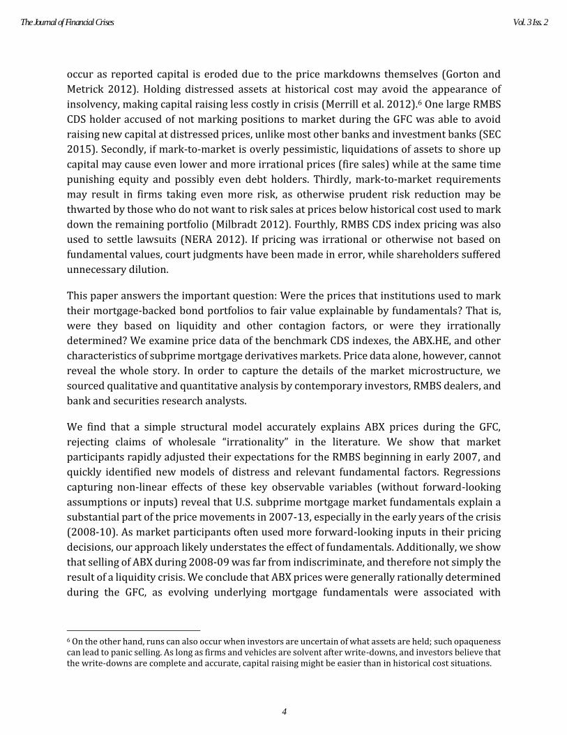
Securitization transforms a portfolio of debt contracts into instruments that have differing

risk profiles from the original underlying contracts through the use of subordination as

credit enhancement.7 A large number of mortgage loans are transferred into a special

purpose vehicle (SPV, Figure 1). Payments from U.S. mortgage loans flowing into RMBS

structures include scheduled interest, plus scheduled (from amortization) and unscheduled

(from prepayments and liquidation proceeds) principal. Agency mortgages dominate the U.S.

securitization market. Because credit risk has been minimized for agency securitizations via

a guarantee issued by the government-sponsored enterprises (GSEs8), prepayment is

modelled as the primary risk and default loss is not considered.

Non-agency mortgages, ineligible for a guarantee from any of the U.S. GSEs, were securitized

into prime jumbo (high quality large loans), Alternative-A (Alt-A, the “best of the worst”

loans), or subprime deals. Payments get contractually divided into the various tranches

(bonds) of the securitization (Figures 1 and 2 and Table 1). The goal of the tranching is

primarily to make the upper tranches, and especially the Class A tranches, unlikely to sustain

any losses, irrespective of mortgage portfolio performance.9 Though the reality is more

complicated than this simple example, for the purposes of this paper one can model

subprime distress by assuming that any losses up to the Class As in the securitized pool of

mortgages are applied up the structure from the lowest tranche first (1 in Figure 1). One can

7 Other credit enhancement mechanisms are used in securitization but are irrelevant in severe distress. (See Goodman et al. (2008).) The following paragraphs describing the subprime RMBS and RMBS index CDS market are loosely based on Saleuddin (2015, chs 2-3). (See Gorton (2009) for a more detailed explanation of subprime, ABX and the GFC.) 8 The three GSEs that issue securitized RMBS are Federal National Mortgage Association (Fannie Mae), Federal Home Loan Mortgage Corporation (Freddie Mac), and the Government National Mortgage Association (Ginnie Mae). They accounted for about half the MBS issuance in the three years preceding the crisis. 9 As we show here, such expectations of being “loss remote” were unrealistic in hindsight.

5


also assume that repayments are allocated to the most senior tranches first (3 in Figure 1)

in order of a prespecified priority, from “first pay” to “penultimate pay” to “last pay.”10 Due

to the high expectations of repayments to the most senior Class A tranches and a low

likelihood of losses being sustained, these have been historically rated AAA, implying almost

zero probability of default.11 During and after the GFC, however, losses often resulted in the

write-down of all of the subordinated (M and B) tranches, resulting in an almost certain

eventual default of many Class A bonds. However, generally the most senior bonds are not

written down, even if the reports by the administrators of the securitization reveal that there

are not enough portfolio assets to repay the bonds at their final maturity. Such impaired Class

A bonds are considered near-defaulted and are rated C or CC.

Investors and hedgers commonly adjusted their exposure to subprime credit and market

risk by being long or short credit default swaps (CDS) referencing four standardized

portfolios, the ABX.HE indices. Traditionally, CDS on corporate credit can be thought of as

credit insurance, offering the protection buyer a cash payment (the Floating Amount) based

on the auction price of an underlying credit instrument (bond or loan) conditioned on the

triggering of a Credit Event, usually a failure to pay a contracted debt payment, or a

bankruptcy. In return, the protection seller receives an ongoing coupon payment (like an

insurance premium) as long as a Credit Event has not occurred. The spread is fixed for the

term of the contract, so the contract can be traded on a price basis.

10 Again, the reality is somewhat more complex, yet adding complexity would not alter the results of this paper. 11 The major ratings categories are Aaa/AAA, Aa/AA, A, Baa/BBB, Ba/BB, B, Caa/CCC, Ca/CC and C. We use the generic labels AAA, BBB and BBB- ratings here. All but the Ca/CC, C and Aaa/AAA have modifiers from 1 (highest) to 3 (lowest quality) or -, flat, and +. For example, BBB- is the rating category above BB+ one below BBB (flat). BBB- and above is considered investment grade. Non-investment grade is any rating BB+ and lower. C is considered default or near default. D and WD are used by some agencies to designate a default.

6


Figure 1: Original deal structure and hypothetical loss case

Source: Authors’ own.

7


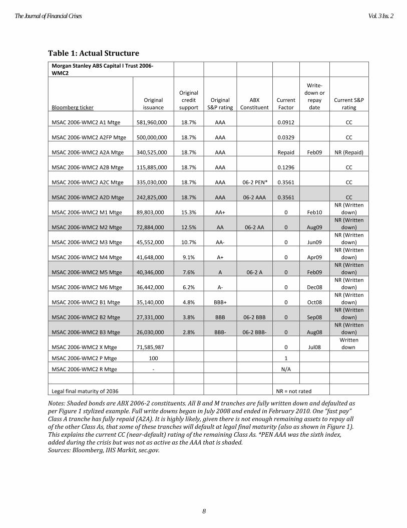
Table 1: Actual Structure

Morgan Stanley ABS Capital I Trust 2006-WMC2

Bloomberg ticker Original issuance

Original credit

support Original

S&P rating ABX

Constituent Current Factor

Write-down or

repay date

Current S&P rating

MSAC 2006-WMC2 A1 Mtge 581,960,000 18.7% AAA 0.0912 CC

MSAC 2006-WMC2 A2FP Mtge 500,000,000 18.7% AAA 0.0329 CC

MSAC 2006-WMC2 A2A Mtge 340,525,000 18.7% AAA Repaid Feb09 NR (Repaid)

MSAC 2006-WMC2 A2B Mtge 115,885,000 18.7% AAA 0.1296 CC

MSAC 2006-WMC2 A2C Mtge 335,030,000 18.7% AAA 06-2 PEN* 0.3561 CC

MSAC 2006-WMC2 A2D Mtge 242,825,000 18.7% AAA 06-2 AAA 0.3561 CC

MSAC 2006-WMC2 M1 Mtge 89,803,000 15.3% AA+ 0 Feb10

NR (Written down)

MSAC 2006-WMC2 M2 Mtge 72,884,000 12.5% AA 06-2 AA 0 Aug09

NR (Written down)

MSAC 2006-WMC2 M3 Mtge 45,552,000 10.7% AA- 0 Jun09

NR (Written down)

MSAC 2006-WMC2 M4 Mtge 41,648,000 9.1% A+ 0 Apr09

NR (Written down)

MSAC 2006-WMC2 M5 Mtge 40,346,000 7.6% A 06-2 A 0 Feb09

NR (Written down)

MSAC 2006-WMC2 M6 Mtge 36,442,000 6.2% A- 0 Dec08

NR (Written down)

MSAC 2006-WMC2 B1 Mtge 35,140,000 4.8% BBB+ 0 Oct08

NR (Written down)

MSAC 2006-WMC2 B2 Mtge 27,331,000 3.8% BBB 06-2 BBB 0 Sep08

NR (Written down)

MSAC 2006-WMC2 B3 Mtge 26,030,000 2.8% BBB- 06-2 BBB- 0 Aug08

NR (Written down)

MSAC 2006-WMC2 X Mtge 71,585,987 0 Jul08

Written down

MSAC 2006-WMC2 P Mtge 100 1

MSAC 2006-WMC2 R Mtge - N/A

Legal final maturity of 2036 NR = not rated

Notes: Shaded bonds are ABX 2006-2 constituents. All B and M tranches are fully written down and defaulted as per Figure 1 stylized example. Full write downs began in July 2008 and ended in February 2010. One “fast pay” Class A tranche has fully repaid (A2A). It is highly likely, given there is not enough remaining assets to repay all of the other Class As, that some of these tranches will default at legal final maturity (also as shown in Figure 1). This explains the current CC (near-default) rating of the remaining Class As. *PEN AAA was the sixth index, added during the crisis but was not as active as the AAA that is shaded. Sources: Bloomberg, IHS Markit, sec.gov.

8


Credit Events and Floating Amounts for ABS CDS differ from those on corporate CDS in that

there is no single Credit Event where the Floating Amount is determined. Instead, as

tranche/bond payments are missed and/or write-downs occur in the underlying bonds,

these losses are paid to the CDS protection buyer.12 Such specialized language is needed to

indicate when payment occurs as most highly rated securitized bonds do not default until

they have not paid a legally required amount of interest or principal, even if the pool

performance implies that they will default with 100% likelihood at a later date. Bankruptcy

or failure to pay a contracted amount rarely occurs in senior (Class A) subprime bonds until

the legal final maturity, which could be as much as 30 years from the time of the realized loss

in the underlying pool (3 in Figure 1).

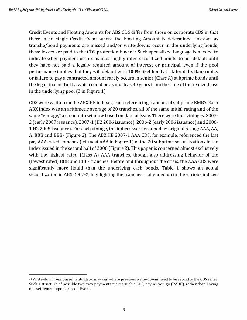
CDS were written on the ABX.HE indexes, each referencing tranches of subprime RMBS. Each

ABX index was an arithmetic average of 20 tranches, all of the same initial rating and of the

same “vintage,” a six-month window based on date of issue. There were four vintages, 2007-

2 (early 2007 issuance), 2007-1 (H2 2006 issuance), 2006-2 (early 2006 issuance) and 2006-

1 H2 2005 issuance). For each vintage, the indices were grouped by original rating: AAA, AA,

A, BBB and BBB- (Figure 2). The ABX.HE 2007-1 AAA CDS, for example, referenced the last

pay AAA-rated tranches (leftmost AAA in Figure 1) of the 20 subprime securitizations in the

index issued in the second half of 2006 (Figure 2). This paper is concerned almost exclusively

with the highest rated (Class A) AAA tranches, though also addressing behavior of the

(lowest rated) BBB and BBB- tranches. Before and throughout the crisis, the AAA CDS were

significantly more liquid than the underlying cash bonds. Table 1 shows an actual

securitization in ABX 2007-2, highlighting the tranches that ended up in the various indices.

12 Write-down reimbursements also can occur, where previous write-downs need to be repaid to the CDS seller. Such a structure of possible two-way payments makes such a CDS, pay-as-you-go (PAUG), rather than having one settlement upon a Credit Event.

9


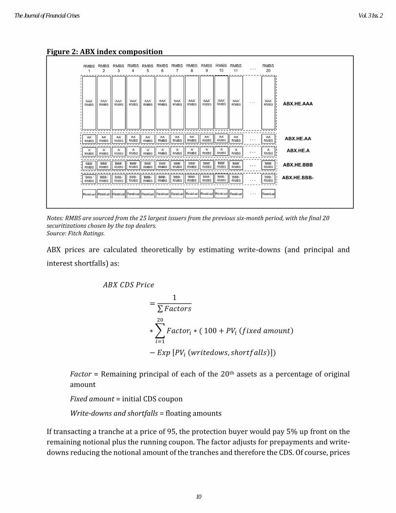
Figure 2: ABX index composition

Notes: RMBS are sourced from the 25 largest issuers from the previous six-month period, with the final 20 securitizations chosen by the top dealers. Source: Fitch Ratings.

ABX prices are calculated theoretically by estimating write-downs (and principal and

interest shortfalls) as:

𝐴𝐵𝑋 𝐶𝐷𝑆 𝑃𝑟𝑖𝑐𝑒

=1

∑ 𝐹𝑎𝑐𝑡𝑜𝑟𝑠

∗ ∑ 𝐹𝑎𝑐𝑡𝑜𝑟𝑖 ∗ ( 100 + 𝑃𝑉𝑖 (𝑓𝑖𝑥𝑒𝑑 𝑎𝑚𝑜𝑢𝑛𝑡)

20

𝑖=1

− 𝐸𝑥𝑝 [𝑃𝑉𝑖 (𝑤𝑟𝑖𝑡𝑒𝑑𝑜𝑤𝑠, 𝑠ℎ𝑜𝑟𝑡𝑓𝑎𝑙𝑙𝑠)])

Factor = Remaining principal of each of the 20th assets as a percentage of original

amount

Fixed amount = initial CDS coupon

Write-downs and shortfalls = floating amounts

If transacting a tranche at a price of 95, the protection buyer would pay 5% up front on the

remaining notional plus the running coupon. The factor adjusts for prepayments and write-

downs reducing the notional amount of the tranches and therefore the CDS. Of course, prices

10


may deviate from rational expectations of the above parameters. The question of how much

deviation occurred in 2008-10 is addressed below.

2.2 The subprime crisis

The late-boom (2006-07) U.S. subprime mortgage originations almost immediately failed

once housing prices stagnated making it difficult for overextended borrowers to refinance

their teaser rate mortgages (Gorton 2009). The ABX indices fell rapidly once the extent of

the deterioration in subprime portfolios became widely known (Figure 3). By the middle of

2007, delinquencies and foreclosures, indicators of future pool losses, rose to unprecedented

levels. Did ABX prices drop too far? There certainly are several reasons why they may have,

such as limits to arbitrage (Shleifer and Vishny 197). Prices can deviate from fair value when

buyers who could normally purchase securities when prices get “too low” are somehow

limited in their capacity to do so, often because of lack of funding. Certainly, funding markets

for all assets, but especially subprime, were failing catastrophically at the time (Gorton 2009;

Gorton and Metrick 2012). Most every financial asset market also collapsed in the following

years 2008-09, hinting that perhaps ABX prices were driven solely by the same macro and

liquidity concerns that affected all markets.

Figure 3: ABX.HE AAA CDS prices, 2006-2010

Source: IHS Markit.

11


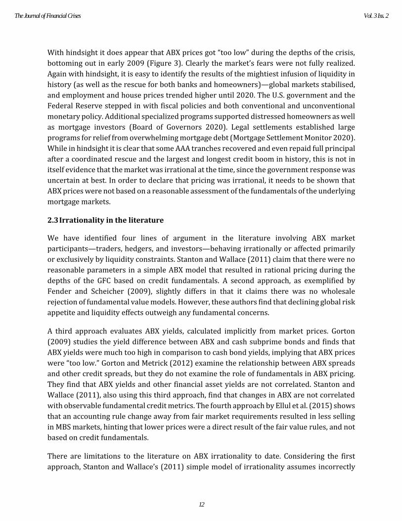
With hindsight it does appear that ABX prices got “too low” during the depths of the crisis,

bottoming out in early 2009 (Figure 3). Clearly the market’s fears were not fully realized.

Again with hindsight, it is easy to identify the results of the mightiest infusion of liquidity in

history (as well as the rescue for both banks and homeowners)—global markets stabilised,

and employment and house prices trended higher until 2020. The U.S. government and the

Federal Reserve stepped in with fiscal policies and both conventional and unconventional

monetary policy. Additional specialized programs supported distressed homeowners as well

as mortgage investors (Board of Governors 2020). Legal settlements established large

programs for relief from overwhelming mortgage debt (Mortgage Settlement Monitor 2020).

While in hindsight it is clear that some AAA tranches recovered and even repaid full principal

after a coordinated rescue and the largest and longest credit boom in history, this is not in

itself evidence that the market was irrational at the time, since the government response was

uncertain at best. In order to declare that pricing was irrational, it needs to be shown that

ABX prices were not based on a reasonable assessment of the fundamentals of the underlying

mortgage markets.

2.3 Irrationality in the literature

We have identified four lines of argument in the literature involving ABX market

participants—traders, hedgers, and investors—behaving irrationally or affected primarily

or exclusively by liquidity constraints. Stanton and Wallace (2011) claim that there were no

reasonable parameters in a simple ABX model that resulted in rational pricing during the

depths of the GFC based on credit fundamentals. A second approach, as exemplified by

Fender and Scheicher (2009), slightly differs in that it claims there was no wholesale

rejection of fundamental value models. However, these authors find that declining global risk

appetite and liquidity effects outweigh any fundamental concerns.

A third approach evaluates ABX yields, calculated implicitly from market prices. Gorton

(2009) studies the yield difference between ABX and cash subprime bonds and finds that

ABX yields were much too high in comparison to cash bond yields, implying that ABX prices

were “too low.” Gorton and Metrick (2012) examine the relationship between ABX spreads

and other credit spreads, but they do not examine the role of fundamentals in ABX pricing.

They find that ABX yields and other financial asset yields are not correlated. Stanton and

Wallace (2011), also using this third approach, find that changes in ABX are not correlated

with observable fundamental credit metrics. The fourth approach by Ellul et al. (2015) shows

that an accounting rule change away from fair market requirements resulted in less selling

in MBS markets, hinting that lower prices were a direct result of the fair value rules, and not

based on credit fundamentals.

There are limitations to the literature on ABX irrationality to date. Considering the first

approach, Stanton and Wallace’s (2011) simple model of irrationality assumes incorrectly

12


that all non-defaulted mortgages repay in full at the end of one year, and that all prepayments

occur before the default rate is applied. To reasonably approximate reality, the default rate

would need to apply for the life of the bond and repayment rates, and default rates and loss

given default would have to match contemporary observed or expected levels. In section four

of this paper we extend their simple model and use more reasonable assumptions to provide

simple yet robust results that fit observed pricing.

Issues with the second and third approach are many, but they distill down to two points: (1)

Pre-2007 econometric models and data cannot be, and were not, used to estimate losses to

the underlying RMBS during and after the GFC, and (2) ABX junior tranches under stress

cannot be analyzed in the same way as senior tranches or corporate CDS. We cover each of

these in the next two subsections.

2.4 Models of ABX distress, a regime change

There are two main types of models used by practitioners to estimate future default losses

in RMBS. Before 2007, an “econometric model” was most common (Goodman et al. 2008).13

Such models were driven by macro and microeconomic factors such as house price

appreciation, interest rates (affecting affordability as well as refinanceability) and

unemployment. The models were fit using historical data and used to predict portfolio

repayments and losses. These models often assumed a strong relationship between house

price appreciation measure (HPA) and prepayment. As long as HPA was positive, default

losses were forecast to be minimal and prepayments very high: often between 30% and 40%,

pre-GFC. With declining HPA, such models can fail catastrophically (Rodriguez 2007). Even

a small decline in borrowers’ equity makes refinancing impossible. The now negative HPA

will no longer be a relevant factor affecting (the now low) prepayments and will not become

a factor again until the mortgages are back above the A level where they can be refinanced.

Therefore, not only did negative HPA cause an immediate halt to prepayments, default losses

were rising as mortgage coupons were rising, refinancing was impossible, and repossessed

houses hit the market causing a negative feedback loop. The old models no longer applied.

Subprime bonds originating in mid-2005 to mid-2007 constituted the majority of those still

outstanding when the GFC hit and were much less creditworthy than subprime bonds issued

previously (Goodman et al. 2008; Acharya et al. 2011; Demyanyk and van Hemert 2011;

Moody’s 2018). The majority of loans in 2006-07 subprime deals had low “teaser” interest

rates that rose to unaffordable levels after two to three years, with the end result that after

the teaser period, the loan would refinance, if HPA would allow it, or default. Surprise

negative HPA was, in fact, the discontinuity that caused the subprime failure. Before late

13 “Econometric models” in this context refer to a very specific use of house price appreciation, interest rates, and other economic variables to model defaults and prepayments.

13


2006, positive HPA drove prepayments. By 2007, negative HPA caused the whole market to

fail. By late 2007, it was clear to most participants that, due to house price falls that had

already occurred, HPA was irrelevant for prepayment rates (Credit Suisse 2008). Only a

tremendous increase in prices would have allowed for any prepayments at all, so changes in

HPA around the new lower level would have no effect. The past could no longer be used as a

guide for future performance and, as such, the old econometric models were quickly

abandoned. HPA became an explicit assumption, rather than formed by an econometric

model (Credit Suisse 2007; JPMorgan 2008; Deutsche Bank 2008b).

When the crisis hit, some variables were (theoretically and, in the eyes, of participants,

practically) no longer relevant, such as HPA and interest rates for prepayment. Expected HPA

began to be used to calculate current and future LTVs to determine the likelihood of default

and loss severity (Barclays Capital 2009). Small changes in HPA were unimportant (Deutsche

Bank 2007).14

New forward-looking “migration” models (Goodman et al. 2008) replaced econometric ones

early in the crisis. These models priced RMBS and ABX using expectations of default rates

and loss severity based on (negative) expected HPA, jurisdictional differences, and very

recent observations of portfolio performance characteristics such as delinquencies and

insolvencies. The relationships between delinquent loans and further distress such as

insolvency, deeper delinquency, and default as well as regional idiosyncrasies regarding

losses given default (LGD, also known as loss severity) were monitored closely, and observed

relationships between these variables became the bases for the new models. Variables such

as current delinquency were used as predictors of further delinquency, “cures” (the debtor

resuming payments), and further distress. It was also quickly realized that further

prepayments in deals where mortgages were “underwater” (LTVs higher than 100%) would

be near zero for some time (Credit Suisse 2008).

2.5 ABX BBB

A four-year CDS that costs 95% (as ABX 06-2 BBB did in 2008) would show a yield of around

10,000-20,000 basis points depending on methodology and precise assumptions. That

spread has little relation to the expected return. At such low prices, mezzanine tranches were

providing almost no information about the riskiness of the subprime securitizations. For

example, JPMorgan (2008) estimated that the BBB and BBB- tranches would barely survive

the year before default losses would need to be paid out, and so were trading as “interest

only” (IO). A protection seller could receive 100–ABX price today, earn a few quarterly

coupons, but be required to pay 100 within one year or two, depending on the exact timing

14 Other parameters often used as risk measures pre-crisis have always been known to be so lagging as to be useless, such as ratings. One year into the crisis, ABX 06-2 AAAs were still rated high investment grade on average (Fender and Scheicher 2009). Currently, the average rating is B- (Moody’s 2018).

14


of the (fully-expected) write-downs. The IRR of such a trade was in the low double digits in

percentage terms if expectations were realized, not 10,000s of basis points.

The changes in price of most junior tranches in 2008-09 reflected the possibility of one more

or one fewer coupon rather than any overall changes in riskiness in the underlying subprime

assets. The BBB indices were insensitive to losses in excess of those that would wipe out the

tranche. Once losses were expected to eventually wipe out the tranche and result in no

principal payment (requiring losses of usually less than 5% of an RMBS), the only cash flows

that would be expected to be paid in the future would be interest payments, and even then

only until complete write-down. Even large positive revisions to loss expectations to

subprime could not have affected tranches about to be completely written down in all

scenarios. That is, traders could have vastly altered their assumptions regarding the

underlying RMBS markets and, therefore, the senior ABX tranches, without it significantly

affecting the BBB market’s returns, which were based on almost certain and total write-

down.

In fact, most of the BBB and BBB- ABX indices never recovered from their quick approach to

near-zero prices (Figure 4). Prices remained close to zero even as AAA subprime indices

rebounded post-crisis. Only one BBB- and two BBB bonds out of the 80 ABX deals retain any

principal, with the rest written down to zero (factors sourced from Bloomberg in October,

2020). By October 2007, the remaining final write-down date was three years hence for ABX

06-1 and 06-2 BBB- and two years hence (June 2009) on average for ABX 07-1 and 07-2 BBB-

. Considering the IO component was the only positive cash flow likely to be earned by most

index investors (other than small amounts possible in 06-1 and 06-2), it can be said that ABX

BBB prices reacted rationally to the subprime crisis in a timely manner. By the middle of

2008, as revisions to the write-down dates occurred, prices changed (Figure 5). That the

yields appeared to behave “strangely” is not proof of pricing irrationality. In this paper we

focus on the price changes of the most senior tranches, which would better reflect the

changes in fundamentals, whether backward or forward looking.

15


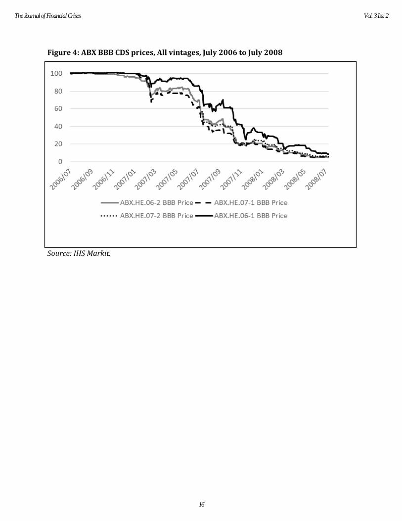
Figure 4: ABX BBB CDS prices, All vintages, July 2006 to July 2008

Source: IHS Markit.

16


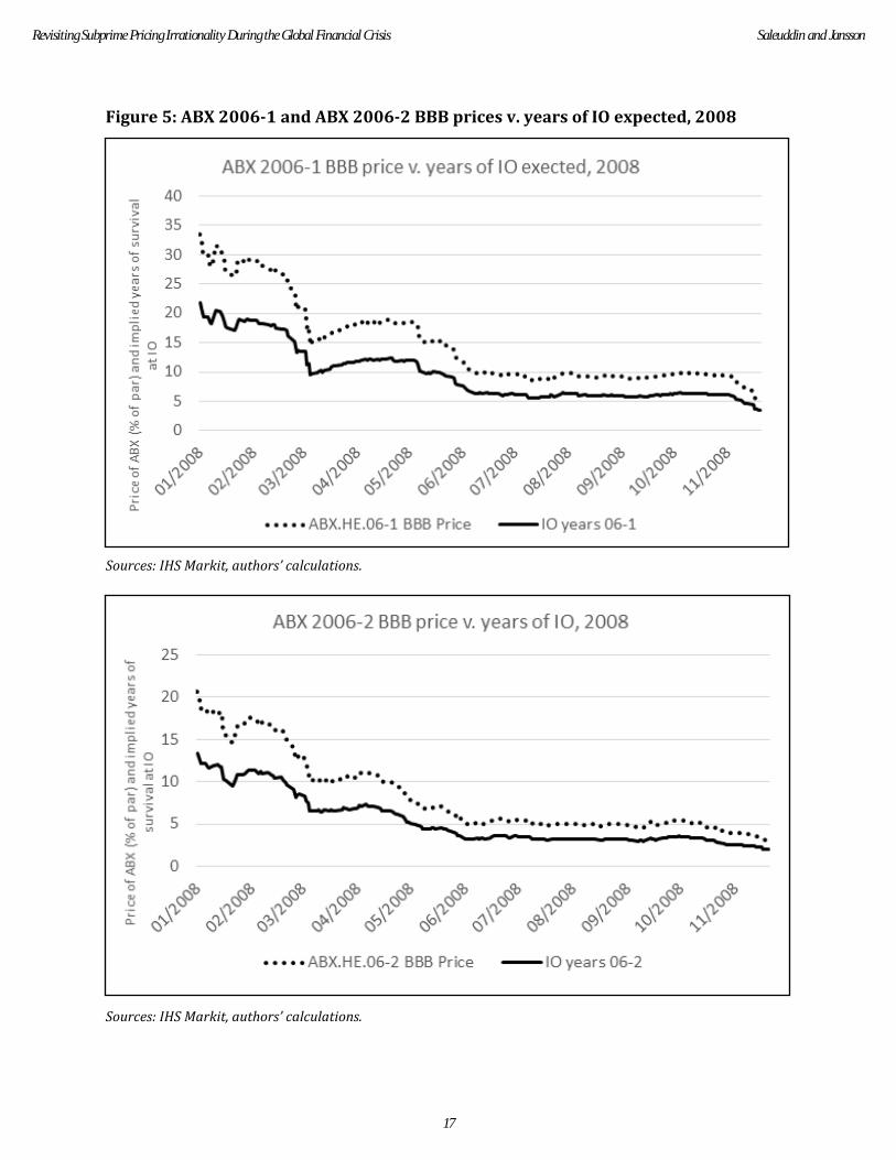
Figure 5: ABX 2006-1 and ABX 2006-2 BBB prices v. years of IO expected, 2008

Sources: IHS Markit, authors’ calculations.

Sources: IHS Markit, authors’ calculations.

17


3. Data

This section describes the data used for our econometric analysis. We obtained prices

directly from the official mark-to-market source for ABX, IHS Markit. All the relevant

measures of credit quality, loss experience, and deal and tranche characteristics were

sourced from Bloomberg. Market and macroeconomic data are from Eikon. The data is at the

monthly frequency, which matches the frequency of available RMBS remit data. The sample

runs from July 2007 to December 2013. The starting point of the sample is conditioned on

the availability of sufficient remit data through Bloomberg for most bonds to construct the

necessary proxies for credit quality. The end date is determined by the fact that ABX prices

start exhibiting very little variance after this point. According to our data, for example, the

07-2 AAA index had price changes in every month in 2013, but the price was largely static

from March 2014 onwards. Prices stabilized as losses became more likely to wipe out some

Class A tranches (primarily in later vintages), or more likely to be repaid in full (primarily in

the earlier vintages), or some combination.

Unlike equities or corporate debt, structured securities such as RMBS do have some

fundamentally important factors that can be used to discern value. Mortgages with LTVs

close to and above 100% and higher delinquencies are more likely to cause distress to the

securitized portfolios, all else being equal. Each month, a certain percentage of delinquencies

migrate from 30 days to 60 days to 90 days to 180 days. Foreclosure often begins after 90

days. If LTVs are low, losses to the pool, even if defaults rise, are unlikely. To model the

expected losses and therefore the prices of subprime bonds and CDS, traders and investors

generally use a range of variables such as those shown in Figure 6: foreclosures,

delinquencies, defaults, and prepayments. More elaborate models project future migration

rates on macroeconomic assumptions.

18


Figure 6: ABX portfolio characteristics by vintage, June 2007-December 2013

Notes: The three-month CDR is annualized. Source: Bloomberg.

In Figure 6, the voluntary CPR (prepayment rate, annualized) refers to voluntary

unscheduled principal payments measured as a share of the pool and very different from

involuntary “repayments” that flow through the RMBS structure due to recoveries on

defaulted mortgages. CDR refers to the annualized default rate—effectively the share of

defaulted mortgages as a percentage of the pool balance. Loss severity is the loss of

remaining mortgage principal after a default.

Our aim was to create a highly parsimonious model while still utilizing the primary variables

used by practitioners at the time of the GFC. While investors and traders would examine the

input variables at the deal/tranche level (or even at the individual mortgage level, we

summarize the credit performance of the ABX.HE indices using the measures aggregated

over the 20 deals in each index. The first of these is average 60+ day delinquencies, which

19


includes loans that are delinquent by more than 60 days, including real estate owned, and

foreclosures. The second variable is average credit support: the balance of more junior

tranches relative to the tranches underlying ABX.HE AAA indices (expressed as a share of

total outstanding balance). Table 2 shows summary statistics of these figures, alongside

ABX.HE AAA prices, for the sample period used in the regressions: July 2007 to December,

2013.15 The data is at a monthly frequency, which matches the frequency of RMBS remits.

15 Before July 2007, Bloomberg does not contain sufficient data for many of the bonds underlying the ABX indices. After December 2013, ABX prices start expressing relatively little variance.

20


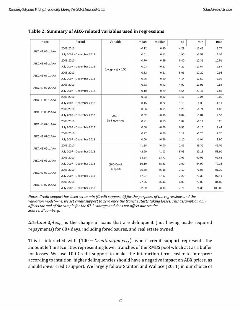
Table 2: Summary of ABX-related variables used in regressions

Index Period Variable mean median sd min max

ABX.HE.06-1 AAA 2008-2010

Δlog(price) x 100

-0.12 0.30 4.29 -11.48 9.77

July 2007 - December 2013 0.01 0.12 1.90 -7.52 3.05

ABX.HE.06-2 AAA 2008-2010 -0.70 0.59 5.40 -12.31 10.51

July 2007 - December 2013 0.03 -0.17 4.21 -12.64 7.87

ABX.HE.07-1 AAA 2008-2010 -0.82 -0.61 5.06 -12.29 9.93

July 2007 - December 2013 -0.26 0.20 4.14 -17.50 7.02

ABX.HE.07-2 AAA 2008-2010 -0.83 -0.42 4.92 -11.91 9.84

July 2007 - December 2013 -0.10 0.29 4.54 -22.47 7.85

ABX.HE.06-1 AAA 2008-2010

Δ60+

Delinquencies

0.33 0.32 1.16 -3.24 3.80

July 2007 - December 2013 0.15 -0.22 1.19 -1.39 4.11

ABX.HE.06-2 AAA 2008-2010 0.56 0.61 1.26 -1.74 4.00

July 2007 - December 2013 0.02 -0.16 0.84 -0.84 2.52

ABX.HE.07-1 AAA 2008-2010 0.71 0.63 1.09 -1.11 3.25

July 2007 - December 2013 0.00 -0.29 0.91 -1.13 2.44

ABX.HE.07-2 AAA 2008-2010 0.77 0.86 1.12 -1.26 2.76

July 2007 - December 2013 0.06 -0.26 1.10 -1.04 3.90

ABX.HE.06-1 AAA 2008-2010

(100-Credit

support)

41.38 40.00 2.43 39.35 48.05

July 2007 - December 2013 42.29 41.03 5.05 39.13 58.99

ABX.HE.06-2 AAA 2008-2010 63.64 63.71 1.93 60.95 66.63

July 2007 - December 2013 69.10 68.63 2.00 64.92 72.25

ABX.HE.07-1 AAA 2008-2010 75.58 75.18 3.19 71.87 81.39

July 2007 - December 2013 87.27 87.37 7.20 73.33 97.41

ABX.HE.07-2 AAA 2008-2010 77.56 76.46 4.03 73.08 84.85

July 2007 - December 2013 92.09 93.15 7.76 74.36 100.00

Notes: Credit support has been set to min (Credit support, 0) for the purposes of the regressions and the valuation model—i.e. we set credit support to zero once the tranche starts taking losses. This assumption only affects the end of the sample for the 07-2 vintage and does not affect our results. Source: Bloomberg.

Δ𝐷𝑒𝑙𝑖𝑛𝑞60𝑝𝑙𝑢𝑠𝑡,𝑖 is the change in loans that are delinquent (not having made required

repayments) for 60+ days, including foreclosures, and real estate owned.

This is interacted with (100 − 𝐶𝑟𝑒𝑑𝑖𝑡 𝑠𝑢𝑝𝑝𝑜𝑟𝑡𝑖,𝑡), where credit support represents the

amount left in securities representing lower tranches of the RMBS pool which act as a buffer

for losses. We use 100-Credit support to make the interaction term easier to interpret:

according to intuition, higher delinquencies should have a negative impact on ABX prices, as

should lower credit support. We largely follow Stanton and Wallace (2011) in our choice of

21


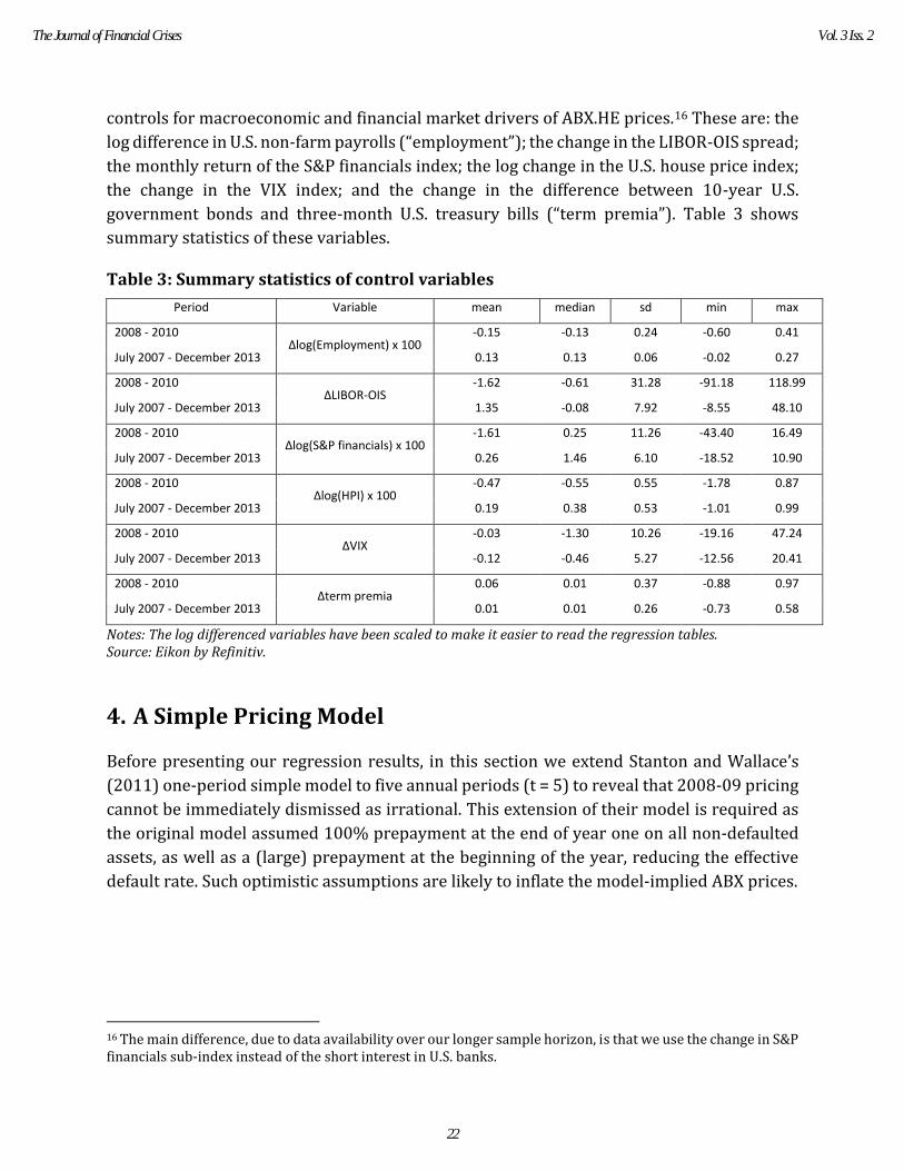
controls for macroeconomic and financial market drivers of ABX.HE prices.16 These are: the

log difference in U.S. non-farm payrolls (“employment”); the change in the LIBOR-OIS spread;

the monthly return of the S&P financials index; the log change in the U.S. house price index;

the change in the VIX index; and the change in the difference between 10-year U.S.

government bonds and three-month U.S. treasury bills (“term premia”). Table 3 shows

summary statistics of these variables.

Table 3: Summary statistics of control variables

Period Variable mean median sd min max

2008 - 2010 Δlog(Employment) x 100

-0.15 -0.13 0.24 -0.60 0.41

July 2007 - December 2013 0.13 0.13 0.06 -0.02 0.27

2008 - 2010 ΔLIBOR-OIS

-1.62 -0.61 31.28 -91.18 118.99

July 2007 - December 2013 1.35 -0.08 7.92 -8.55 48.10

2008 - 2010 Δlog(S&P financials) x 100

-1.61 0.25 11.26 -43.40 16.49

July 2007 - December 2013 0.26 1.46 6.10 -18.52 10.90

2008 - 2010 Δlog(HPI) x 100

-0.47 -0.55 0.55 -1.78 0.87

July 2007 - December 2013 0.19 0.38 0.53 -1.01 0.99

2008 - 2010 ΔVIX

-0.03 -1.30 10.26 -19.16 47.24

July 2007 - December 2013 -0.12 -0.46 5.27 -12.56 20.41

2008 - 2010 Δterm premia

0.06 0.01 0.37 -0.88 0.97

July 2007 - December 2013 0.01 0.01 0.26 -0.73 0.58

Notes: The log differenced variables have been scaled to make it easier to read the regression tables. Source: Eikon by Refinitiv.

4. A Simple Pricing Model

Before presenting our regression results, in this section we extend Stanton and Wallace’s

(2011) one-period simple model to five annual periods (t = 5) to reveal that 2008-09 pricing

cannot be immediately dismissed as irrational. This extension of their model is required as

the original model assumed 100% prepayment at the end of year one on all non-defaulted

assets, as well as a (large) prepayment at the beginning of the year, reducing the effective

default rate. Such optimistic assumptions are likely to inflate the model-implied ABX prices.

16 The main difference, due to data availability over our longer sample horizon, is that we use the change in S&P financials sub-index instead of the short interest in U.S. banks.

22


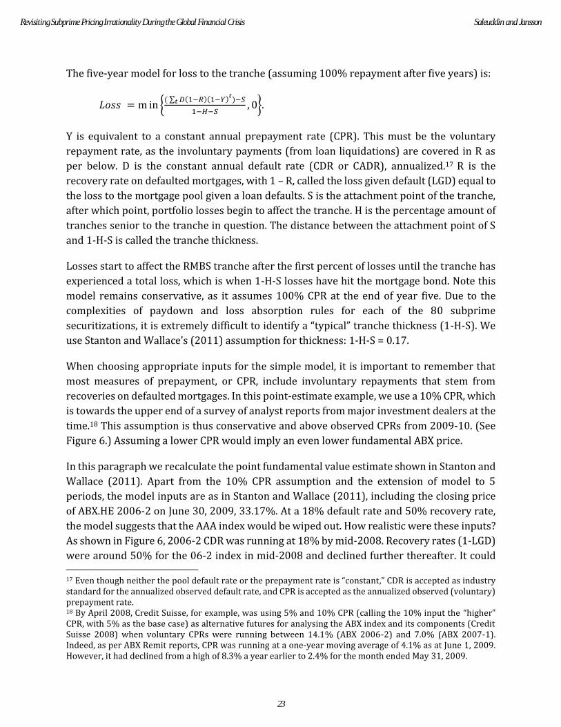
The five-year model for loss to the tranche (assuming 100% repayment after five years) is:

𝐿𝑜𝑠𝑠 = m in {( ∑ 𝐷(1−𝑅)(1−𝑌)𝑡

𝑡)−𝑆

1−𝐻−𝑆, 0}.

Y is equivalent to a constant annual prepayment rate (CPR). This must be the voluntary

repayment rate, as the involuntary payments (from loan liquidations) are covered in R as

per below. D is the constant annual default rate (CDR or CADR), annualized.17 R is the

recovery rate on defaulted mortgages, with 1 – R, called the loss given default (LGD) equal to

the loss to the mortgage pool given a loan defaults. S is the attachment point of the tranche,

after which point, portfolio losses begin to affect the tranche. H is the percentage amount of

tranches senior to the tranche in question. The distance between the attachment point of S

and 1-H-S is called the tranche thickness.

Losses start to affect the RMBS tranche after the first percent of losses until the tranche has

experienced a total loss, which is when 1-H-S losses have hit the mortgage bond. Note this

model remains conservative, as it assumes 100% CPR at the end of year five. Due to the

complexities of paydown and loss absorption rules for each of the 80 subprime

securitizations, it is extremely difficult to identify a “typical” tranche thickness (1-H-S). We

use Stanton and Wallace’s (2011) assumption for thickness: 1-H-S = 0.17.

When choosing appropriate inputs for the simple model, it is important to remember that

most measures of prepayment, or CPR, include involuntary repayments that stem from

recoveries on defaulted mortgages. In this point-estimate example, we use a 10% CPR, which

is towards the upper end of a survey of analyst reports from major investment dealers at the

time.18 This assumption is thus conservative and above observed CPRs from 2009-10. (See

Figure 6.) Assuming a lower CPR would imply an even lower fundamental ABX price.

In this paragraph we recalculate the point fundamental value estimate shown in Stanton and

Wallace (2011). Apart from the 10% CPR assumption and the extension of model to 5

periods, the model inputs are as in Stanton and Wallace (2011), including the closing price

of ABX.HE 2006-2 on June 30, 2009, 33.17%. At a 18% default rate and 50% recovery rate,

the model suggests that the AAA index would be wiped out. How realistic were these inputs?

As shown in Figure 6, 2006-2 CDR was running at 18% by mid-2008. Recovery rates (1-LGD)

were around 50% for the 06-2 index in mid-2008 and declined further thereafter. It could

17 Even though neither the pool default rate or the prepayment rate is “constant,” CDR is accepted as industry standard for the annualized observed default rate, and CPR is accepted as the annualized observed (voluntary) prepayment rate. 18 By April 2008, Credit Suisse, for example, was using 5% and 10% CPR (calling the 10% input the “higher” CPR, with 5% as the base case) as alternative futures for analysing the ABX index and its components (Credit Suisse 2008) when voluntary CPRs were running between 14.1% (ABX 2006-2) and 7.0% (ABX 2007-1). Indeed, as per ABX Remit reports, CPR was running at a one-year moving average of 4.1% as at June 1, 2009. However, it had declined from a high of 8.3% a year earlier to 2.4% for the month ended May 31, 2009.

23


be argued that a five-period distress model is too aggressive, yet a three-period model does

not significantly alter the results. Three stressful years would result in a loss of more than

50% in the ABX 2006-2 index. Comparing 0% and 48% model values to the market price on

Jun 30, 2008, of 33.17% reveals that market prices could, to some extent, be approximated

by a very simple pricing model. Simple models are unlikely to be able to show that the market

was completely detached from reality even at the depths of the GFC.

Figure 7 below reinforces the preliminary finding that ABX prices could be explained by

fundamentals. Here, we compare the ABX price on the simple five-period model-implied

price. We use S, R and CDRs contained in the ABX remit data releases for January 2008 to

October 2010. Note that fundamental data lagged somewhat due to the time taken between

actions within the mortgage pools and the reporting in the remit data that is sourced from

deal trustee reports. Simple eyeballing of the data suggests that the prices bore a relationship

to this very crude proxy of fundamentals. The right-hand-side data shows, however, that

model price can be par even when market price is low. Three influences account for this,

Firstly, when the market price is high and fundamental impairments are not expected, the

prices should vary according to liquidity and risk preferences. The second issue is that the

simple model’s specification results in a highly volatile price. If the CDR for the month is

temporarily lower than recent periods, the price will be abnormally high. Thirdly, once losses

hit the pools, CDRs will be less responsible for price decreases. This indeed occurred in the

ABX markets. CDRs fell as losses rose after October 2010. Losses are shown still accruing to

the bonds even though CDRs have fallen from their 2009-11 highs. Most often, however,

when market prices were well below par, significant losses were expected in this simple

model. In fact, the regression relationship is positive and significant at the 99.9% level, with

an R2 of 68%.

24


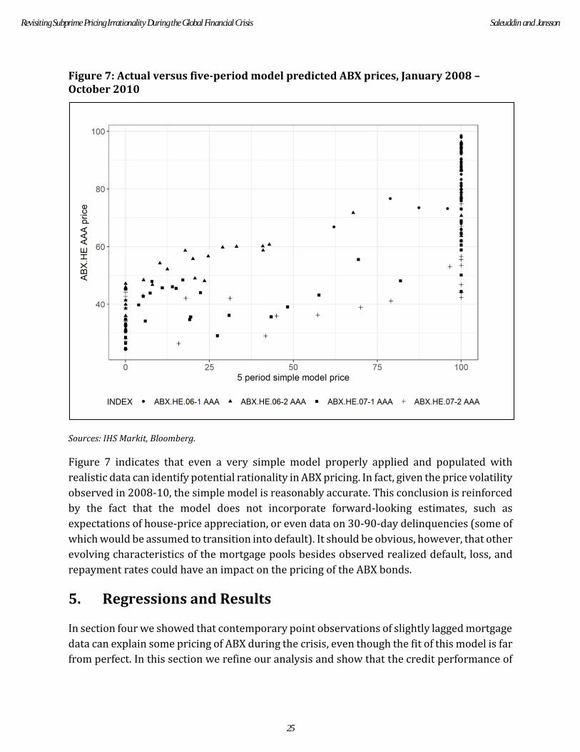
Figure 7: Actual versus five-period model predicted ABX prices, January 2008 – October 2010

Sources: IHS Markit, Bloomberg.

Figure 7 indicates that even a very simple model properly applied and populated with

realistic data can identify potential rationality in ABX pricing. In fact, given the price volatility

observed in 2008-10, the simple model is reasonably accurate. This conclusion is reinforced

by the fact that the model does not incorporate forward-looking estimates, such as

expectations of house-price appreciation, or even data on 30-90-day delinquencies (some of

which would be assumed to transition into default). It should be obvious, however, that other

evolving characteristics of the mortgage pools besides observed realized default, loss, and

repayment rates could have an impact on the pricing of the ABX bonds.

5. Regressions and Results

In section four we showed that contemporary point observations of slightly lagged mortgage

data can explain some pricing of ABX during the crisis, even though the fit of this model is far

from perfect. In this section we refine our analysis and show that the credit performance of

25


assets underlying the indices were significant drivers of ABX prices, while not dismissing the

role played by broader macroeconomic factors.

In previous literature that econometrically examines the drivers of ABX prices, regressions

typically assume a linear relationship between fundamentals and senior index tranches (e.g.

Stanton and Wallace, 2011). This approach has shortcomings, as senior tranches only start

absorbing losses significantly after losses (driven by delinquencies) have started to

accumulate to junior and mezzanine tranches. Losses affecting junior tranches reduce the

credit support (which can be thought of as “loss-absorbing buffers”) of senior tranches,

which should be reflected in their pricing. But it is only after credit support is expected to be

eroded that the mapping of losses to ABX prices should be expected to be strong. By

accounting for this feature by using a simple interaction term in a standard pooled panel

regression specification, we show below that fundamentals did play a role in the pricing of

ABX indices. This contrasts with findings by Fender and Scheicher (2009) as well as those by

Stanton and Wallace (2011), who argue that subprime AAA RMBS CDS indexes reacted

primarily to systemic risk and developments in broader financial markets, while underlying

fundamentals had a small role to play.

To incorporate nonlinearities discussed above, we interact the level of credit support for

each vintage with the change in delinquencies. This parsimoniously captures a key feature

of CDS pricing: the prices should become more sensitive to credit deterioration as the loss-

absorbing buffer (credit support) deteriorates. Our baseline regression specification is as

follows:

Δ𝐴𝐵𝑋𝑡,𝑖 = 𝛼 + 𝛽1Δ𝐴𝐵𝑋𝑡−1,𝑖 + 𝛽2Δ𝐷𝑒𝑙𝑖𝑛𝑞60𝑝𝑙𝑢𝑠𝑡,𝑖 ∗ (100 − 𝐶𝑟𝑒𝑑𝑖𝑡 𝑠𝑢𝑝𝑝𝑜𝑟𝑡𝑡,𝑖)

+ 𝜸𝟏′ 𝑿𝑡

𝑐𝑜𝑛𝑡𝑟𝑜𝑙𝑠 + 𝜖𝑡,𝑖

The variables here are as discussed in section 3. Recall that in this specification, Δ𝐴𝐵𝑋𝑡,𝑖 is

the log change in price of the AAA ABX.HE index i in month t, where i represents the vintage

(06-1, 06-2, etc.). 𝑿𝑡𝑐𝑜𝑛𝑡𝑟𝑜𝑙𝑠 includes market and macroeconomic controls, as specified above

in section 3.

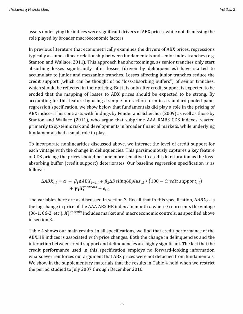
Table 4 shows our main results. In all specifications, we find that credit performance of the

ABX.HE indices is associated with price changes. Both the change in delinquencies and the

interaction between credit support and delinquencies are highly significant. The fact that the

credit performance used in this specification employs no forward-looking information

whatsoever reinforces our argument that ABX prices were not detached from fundamentals.

We show in the supplementary materials that the results in Table 4 hold when we restrict

the period studied to July 2007 through December 2010.

26


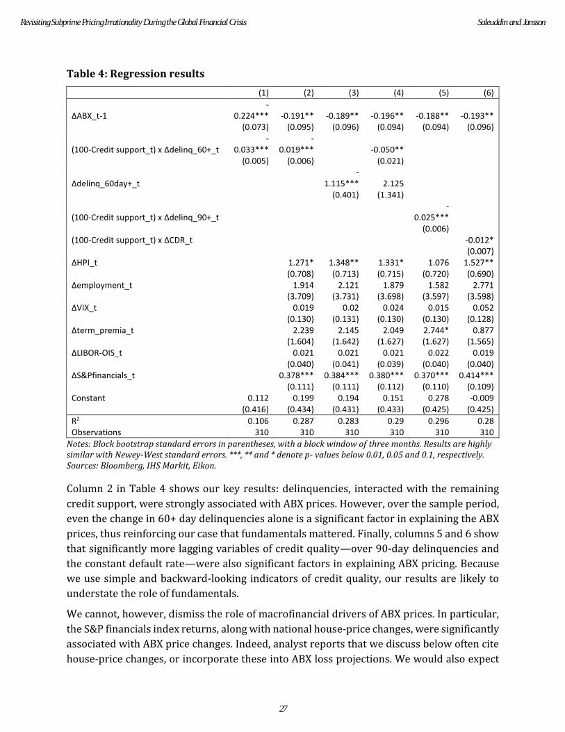
Table 4: Regression results

(1) (2) (3) (4) (5) (6)

ΔABX_t-1 -

0.224*** -0.191** -0.189** -0.196** -0.188** -0.193**

(0.073) (0.095) (0.096) (0.094) (0.094) (0.096)

(100-Credit support_t) x Δdelinq_60+_t -

0.033*** -

0.019*** -0.050** (0.005) (0.006) (0.021)

Δdelinq_60day+_t

-1.115*** 2.125

(0.401) (1.341)

(100-Credit support_t) x Δdelinq_90+_t

-0.025***

(0.006) (100-Credit support_t) x ΔCDR_t -0.012*

(0.007) ΔHPI_t 1.271* 1.348** 1.331* 1.076 1.527**

(0.708) (0.713) (0.715) (0.720) (0.690) Δemployment_t 1.914 2.121 1.879 1.582 2.771

(3.709) (3.731) (3.698) (3.597) (3.598) ΔVIX_t 0.019 0.02 0.024 0.015 0.052

(0.130) (0.131) (0.130) (0.130) (0.128) Δterm_premia_t 2.239 2.145 2.049 2.744* 0.877

(1.604) (1.642) (1.627) (1.627) (1.565) ΔLIBOR-OIS_t 0.021 0.021 0.021 0.022 0.019

(0.040) (0.041) (0.039) (0.040) (0.040) ΔS&Pfinancials_t 0.378*** 0.384*** 0.380*** 0.370*** 0.414***

(0.111) (0.111) (0.112) (0.110) (0.109) Constant 0.112 0.199 0.194 0.151 0.278 -0.009 (0.416) (0.434) (0.431) (0.433) (0.425) (0.425)

R2 0.106 0.287 0.283 0.29 0.296 0.28 Observations 310 310 310 310 310 310

Notes: Block bootstrap standard errors in parentheses, with a block window of three months. Results are highly similar with Newey-West standard errors. ***, ** and * denote p- values below 0.01, 0.05 and 0.1, respectively. Sources: Bloomberg, IHS Markit, Eikon.

Column 2 in Table 4 shows our key results: delinquencies, interacted with the remaining

credit support, were strongly associated with ABX prices. However, over the sample period,

even the change in 60+ day delinquencies alone is a significant factor in explaining the ABX

prices, thus reinforcing our case that fundamentals mattered. Finally, columns 5 and 6 show

that significantly more lagging variables of credit quality—over 90-day delinquencies and

the constant default rate—were also significant factors in explaining ABX pricing. Because

we use simple and backward-looking indicators of credit quality, our results are likely to

understate the role of fundamentals.

We cannot, however, dismiss the role of macrofinancial drivers of ABX prices. In particular,

the S&P financials index returns, along with national house-price changes, were significantly

associated with ABX price changes. Indeed, analyst reports that we discuss below often cite

house-price changes, or incorporate these into ABX loss projections. We would also expect

27


there to be a strong link between the S&P financials index and ABX.HE indices, given the

importance of RMBS in driving financial sector losses.

We know from the theory that pricing is based on expectations, and not simply on

observations of historical data. Table 5 reveals that the simple pricing model outlined in

section 4 helps predict ABX prices. Here, we compare the ABX price with the simple five-

period model component depicting the implied reduction in ABX principal: (( ∑ 𝐷(1 −𝑡

𝑅)(1 − 𝑌)𝑡) − 𝑆)/(1 − 𝐻 − 𝑆).19 We are intentionally conservative in our assumptions here,

because there is a plethora of potential models or forward-looking variables that, ex post,

could be used to justify asset prices. Our model only uses backward-looking data to estimate

future defaults. Faster moving indicators of upcoming defaults, such as macroeconomic

variables, enter the regressions separately, and even 60+ day delinquencies, which contain

more forward-looking information than other pricing model inputs, only enter the

regression in column 3.

Table 5: Regression results with simple model

(1) (2) (3)

ΔABX_t-1 -0.180*** -0.189** -0.191**

(0.074) (0.095) (0.094) Δmodelled_loss_t -10.481*** -4.917* -4.855*

(2.539) (2.799) (2.790) (100-Credit support_t) x Δdelinq_60+_t -0.019***

(0.006) ΔHPI_t 1.726** 1.018

(0.687) (0.713) Δemployment_t 2.274 1.049

(3.491) (3.535) ΔVIX_t 0.059 0.03

(0.127) (0.128) Δterm_premia_t 0.889 2.164

(1.564) (1.571) ΔLIBOR-OIS_t 0.017 0.02

(0.040) (0.041) ΔS&Pfinancials_t 0.425*** 0.379***

(0.108) (0.107) Constant -0.300 0.261 (0.418) (0.417)

R2 0.067 0.277 0.294 Observations 310 310 310

Notes: The valuation denotes the model-implied loss, on which we do not bound between 0 and 1. Block bootstrap standard errors in parentheses, with a block window of three months. Results are highly similar with Newey-West standard errors. ***, ** and * denote p-values below 0.01, 0.05 and 0.1, respectively. Sources: Bloomberg, IHS Markit, Eikon.

19 This model-implied reduction in principal might be greater than 1, which can be interpreted analogously to shadow prices, as the likelihood and severity of actual losses: the greater the implied loss in principal, the more severe actual write-downs are expected to be.

28


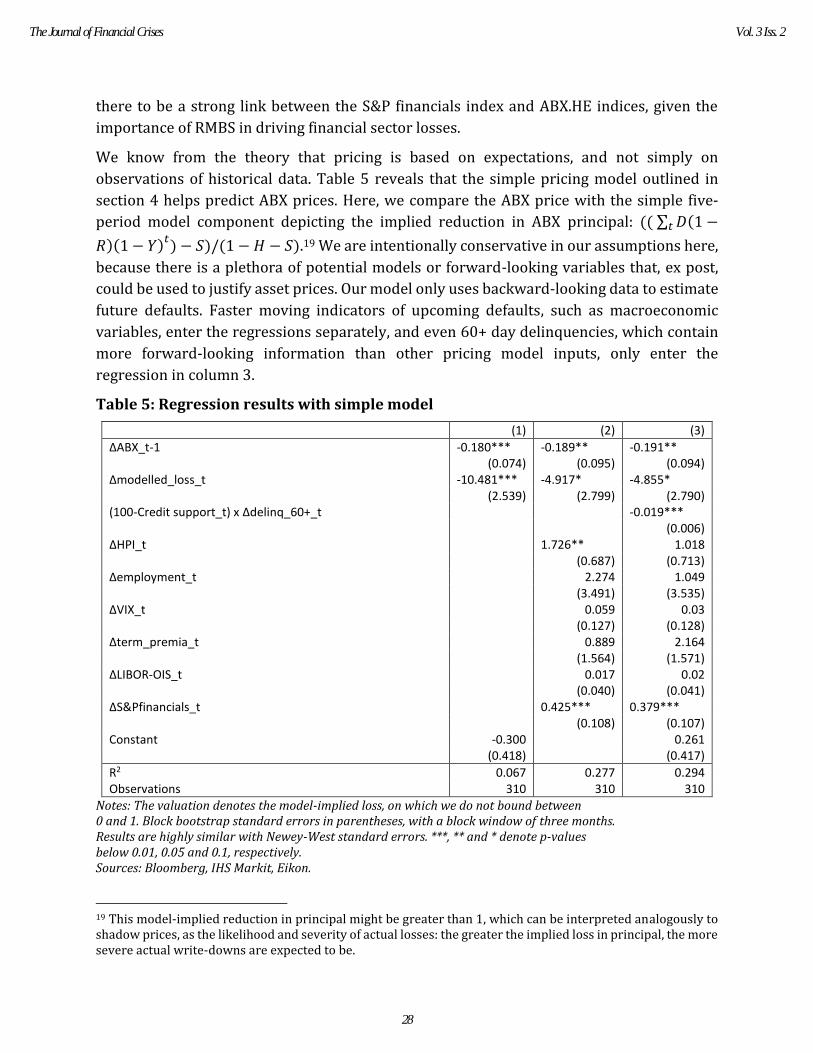
To examine nonlinearities in ABX pricing through a different lens, we estimate quantile

regressions to study how our explanatory variables relate to pricing at different quantiles of

ABX.HE index returns. Our results, shown in Table 6, provide further support of our key

arguments above. In months with the largest ABX price declines (10th and 20th percentiles),

prices were associated with the deterioration in credit quality. This is supported by the

significant interaction term with delinquencies and credit support. This result remains the

same if we only include delinquencies. Additionally, price changes were significantly larger

after credit support had eroded. This is evidenced by the declining coefficient for credit

support as we move to lower quantiles of ABX price changes, which is in line with intuition

about the importance of “loss-absorbing buffers” in non-agency RMBS pricing.

Of course, quantile regression results based on a modest sample size should be interpreted

with caution. It is worth noting, however, that including the intercept term in the regressions

absorbs a significant portion of the variance in ABX prices in this sample, thus possibly

biasing the results against the hypothesis that fundamentals mattered for ABX pricing. If we

remove the intercept, the coefficients for delinquencies become more significant.

Table 6: Quantile regression results with ABX index price changes as the dependent variable

Quantile

0.1 0.2 0.3 0.4 0.5 0.6 0.7 0.8 0.9

ΔABX_t-1 -0.183 -0.186** -0.201 -0.13 -0.143 -0.220** -0.239*** -0.291*** -0.242** (0.082) (0.093) (0.152) (0.170) (0.121) (0.081) (0.062) (0.063) (0.095) (100-Credit support_t) x Δdelinq_60+_t -0.033**

-0.026*** -0.014 -0.005 -0.011 -0.009** -0.003 -0.008* -0.014*

(0.015) (0.013) (0.012) (0.010) (0.007) (0.006) (0.005) (0.006) (0.008) (100-Credit support_t) -0.095***

-0.060*** -0.040* -0.004 0.004 0.021 0.034** 0.041** 0.045

(0.025) (0.025) (0.025) (0.020) (0.016) (0.016) (0.017) (0.021) (0.036) ΔHPI_t 1.455 1.64 1.051 1.135 0.649 0.834 0.983 0.824 0.697 (0.933) (1.064) (1.146) (1.086) (0.900) (0.765) (0.723) (0.882) (1.145)

Δemployment_t 11.786*** 9.767* 10.554** 4.419 -4.336 -8.139* -10.355*** -10.647**

-17.919***

(4.958) (4.727) (5.777) (6.621) (5.728) (4.391) (3.482) (3.785) (4.986) ΔVIX_t -0.131 -0.114 0.012 -0.134 -0.045 0.082 0.217** 0.332*** 0.433** (0.161) (0.141) (0.163) (0.200) (0.195) (0.154) (0.128) (0.115) (0.161) Δterm_premia_t 3.207** 0.756 1.476 -0.818 0.087 1.779* -0.075 1.183 1.074 (2.318) (2.054) (2.271) (2.193) (1.881) (1.610) (1.439) (1.624) (1.781) ΔLIBOR-OIS_t 0.016 0.0002 0.003 0.036 0.011 -0.027 -0.014 -0.023 -0.024 (0.085) (0.092) (0.094) (0.082) (0.058) (0.043) (0.033) (0.031) (0.035) ΔS&Pfinancials_t 0.268 0.321*** 0.313*** 0.346** 0.366** 0.463*** 0.551*** 0.564*** 0.806*** (0.107) (0.112) (0.139) (0.195) (0.203) (0.156) (0.115) (0.115) (0.163) Constant -1.492 -1.78 -1.051 -0.788 0.619 0.68 0.98 2.061 4.809** (1.768) (1.570) (1.485) (1.266) (1.044) (1.082) (1.235) (1.551) (2.729)

Notes: The lowest quantile (0.1) denotes the lowest (most negative) decile of returns of the ABX index, whereas the highest quantile (0.9) denotes the highest return decile. Block bootstrap standard errors in parentheses, with a block window of three months. Results are highly similar with Newey-West standard errors. ***, ** and * denote p-values below 0.01, 0.05 and 0.1, respectively. Sources: Bloomberg, IHS Markit, Eikon.

29


6. Market Predictions

Recall that our econometric models use only contemporary, yet backward-looking, portfolio

performance characteristics to measure the role of fundamentals in ABX pricing. In reality,

market participants also relied on forward-looking models.20 We have evidence that dealers

often thought the fundamentals would get much worse than they actually did in 2010

through to the present. Generally, in finance scholarship, expectations are difficult if not

impossible to measure, but in this case we have evidence from analyst publications that show

that realistic parameters could be identified that would indicate that pricing for indices was

reasonably efficient during the GFC. Rational (at the time) but defensive forward-looking

CPRs, CDRs, and RRs can easily be identified in most ABX pricing during the crisis.21 Some

analysts were clearly closer to the mark than others. In March 2008, JPMorgan (2008)

thought that a market-implied 31.3% collateral loss for late 2006 origination was likely too

conservative. Deutsche Bank (2008a) was more on the mark with an estimate of 38%, almost

spot on the final loss expected by Moody’s in 2018. Voluntary CPRs were expected to be

around 10% for the foreseeable future, while loss severity was expected to maintain lofty

heights 60-80% for the same late-2006 originations. Though the firm thought market prices

were too low, JPMorgan’s models showed AAA ABX prices significantly below par for 07-2

(69.95% of par), 07-1 (71.62% of par) and 06-2 (90.41% of par), 17 to 20 points higher than

the market. As 2008 went on, however, JP Morgan dropped their theoretical values in their

bearish scenario by approximately 10 points for all AAAs other than 06-1, and by 15-20

points in early 2009. In early 2010, Barclays Capital thought that market prices of 88 (06-1),

57 (06-2), 46 (07-1), and 44 (07-2) would yield 5% to 8% IRRs using their baseline portfolio

performance assumptions. Using migration models, Barclays Capital (2009) in early 2009

expected 85% of 2007 originations to default, as approximately 4.5 percentage points of

always current borrowers rolled to delinquent every month during 2008. Barclays Capital

(2010) saw potential returns to 2007 vintage subprime bonds in early 2010 to be between

0% and 1% on a yield-to-maturity basis in their stressed scenario. With current LTVs

significantly above 100% in subprime mortgage pools, defaults would continue high and

prepayments would fall.

Scholars have argued that ABX price declines revealed that there were risks in the subprime

market, but not where those risks lay (Gorton 2009). Indiscriminate selling should put equal

pressure on outwardly similar assets. However, the ABX AAA tranches behaved differently

depending on their fundamentals. It is also evident from the market prices that there was

20 For example, already in August 2007, Credit Suisse (2007a) presented loss projections on ABX indices based on roll rate models and econometric models, both of which used unemployment and house-price projections as additional inputs. 21 Barclays Capital (2010) annual outlook projected overall subprime lifetime loss expectation as a % of original balance to be 53% (based on 10% drop in Case-Shiller national HPA).

30


differentiation between the different ratings categories within and between the vintages.

BBB tranche indices indicated a complete and almost immediate write-down of all bonds for

securitizations originated in late 2006 and early 2007, but prices were somewhat higher for

BBBs for the earlier vintages, where subordination was much higher due to earlier

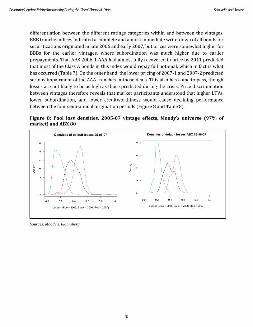
prepayments. That ABX 2006-1 AAA had almost fully recovered in price by 2011 predicted

that most of the Class A bonds in this index would repay full notional, which in fact is what

has occurred (Table 7). On the other hand, the lower pricing of 2007-1 and 2007-2 predicted

serious impairment of the AAA tranches in those deals. This also has come to pass, though

losses are not likely to be as high as those predicted during the crisis. Price discrimination

between vintages therefore reveals that market participants understood that higher LTVs,

lower subordination, and lower creditworthiness would cause declining performance

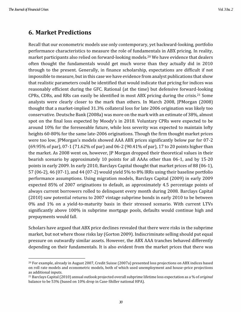
between the four semi-annual origination periods (Figure 8 and Table 8).

Figure 8: Pool loss densities, 2005-07 vintage effects, Moody’s universe (97% of market) and ABX 80

Sources: Moody’s, Bloomberg.

31


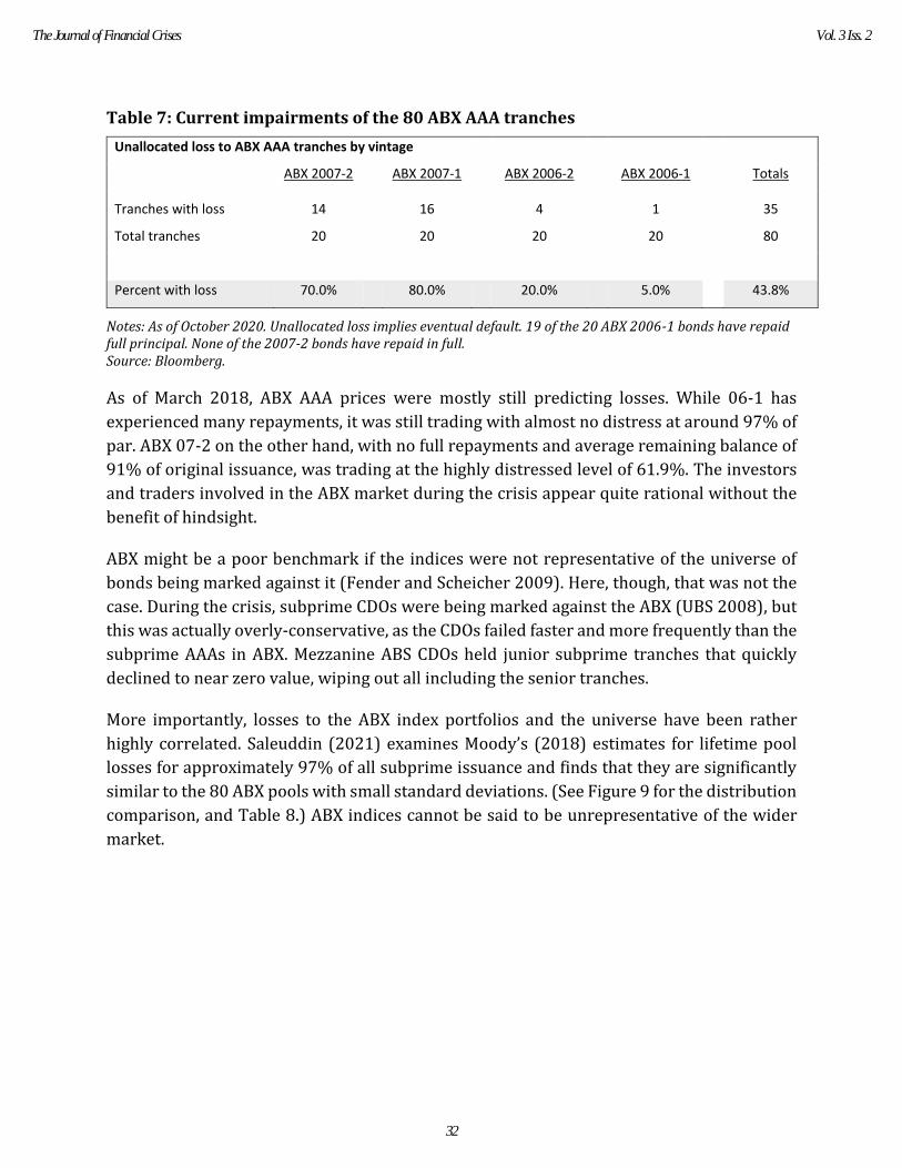
Table 7: Current impairments of the 80 ABX AAA tranches

Unallocated loss to ABX AAA tranches by vintage

ABX 2007-2 ABX 2007-1 ABX 2006-2 ABX 2006-1 Totals

Tranches with loss 14 16 4 1 35

Total tranches 20 20 20 20 80

Percent with loss 70.0% 80.0% 20.0% 5.0% 43.8%

Notes: As of October 2020. Unallocated loss implies eventual default. 19 of the 20 ABX 2006-1 bonds have repaid full principal. None of the 2007-2 bonds have repaid in full. Source: Bloomberg.

As of March 2018, ABX AAA prices were mostly still predicting losses. While 06-1 has

experienced many repayments, it was still trading with almost no distress at around 97% of

par. ABX 07-2 on the other hand, with no full repayments and average remaining balance of

91% of original issuance, was trading at the highly distressed level of 61.9%. The investors

and traders involved in the ABX market during the crisis appear quite rational without the

benefit of hindsight.

ABX might be a poor benchmark if the indices were not representative of the universe of

bonds being marked against it (Fender and Scheicher 2009). Here, though, that was not the

case. During the crisis, subprime CDOs were being marked against the ABX (UBS 2008), but

this was actually overly-conservative, as the CDOs failed faster and more frequently than the

subprime AAAs in ABX. Mezzanine ABS CDOs held junior subprime tranches that quickly

declined to near zero value, wiping out all including the senior tranches.

More importantly, losses to the ABX index portfolios and the universe have been rather

highly correlated. Saleuddin (2021) examines Moody’s (2018) estimates for lifetime pool

losses for approximately 97% of all subprime issuance and finds that they are significantly

similar to the 80 ABX pools with small standard deviations. (See Figure 9 for the distribution

comparison, and Table 8.) ABX indices cannot be said to be unrepresentative of the wider

market.

32


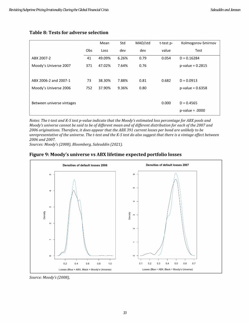
Table 8: Tests for adverse selection

Obs

Mean

Loss

Std

dev

MAD/std

dev

t-test p-

value

Kolmogorov-Smirnov

Test

ABX 2007-2 41 49.09% 6.26% 0.79 0.054 D = 0.16284

Moody’s Universe 2007 371 47.02% 7.64% 0.76 p-value = 0.2815

ABX 2006-2 and 2007-1 73 38.30% 7.88% 0.81 0.682 D = 0.0913

Moody’s Universe 2006 752 37.90% 9.36% 0.80 p-value = 0.6358

Between universe vintages 0.000 D = 0.4565

p-value = .0000

Notes: The t-test and K-S test p-value indicate that the Moody’s estimated loss percentage for ABX pools and Moody’s universe cannot be said to be of different mean and of different distribution for each of the 2007 and 2006 originations. Therefore, it does appear that the ABX 391 current losses per bond are unlikely to be unrepresentative of the universe. The t-test and the K-S test do also suggest that there is a vintage effect between 2006 and 2007. Sources: Moody’s (2008), Bloomberg, Saleuddin (2021).

Figure 9: Moody’s universe vs ABX lifetime expected portfolio losses

Source: Moody’s (2008),

33


7. Conclusions

Deterioration in subprime fundamentals initiated the GFC. The “run on repo” and other

leveraged vehicles then forced the sale of these and other financial assets to repay

collateralized short-term lenders and their investors, such as money market funds. During

the depths of the crisis it appeared, at least in hindsight, that liquidity concerns overwhelmed

fundamental values, perhaps due to the limits of arbitrage. Many scholars and practitioners

conclude that the “fire sale” pricing of the ABX indices, in particular, was irrational. Such

“irrational” pricing forced holders of RMBS to mark down their investments, causing

artificially low equity levels for banks and severe under-collateralization for others such as

the insurance giant, AIG (Blankfein 2010). The assumption that ABX prices were irrational

and the observation that such prices were used to estimate impairment to RMBS investments

led to claims that mark to market exacerbated the GFC. The logical conclusion for some is

that fair value accounting should be ignored during crises.

It is not uncommon, and perhaps expected, that we should see ex post that there is more

downside pressure in the short run in crisis than in the long run, and the common equity

indices performed similarly. ABX prices did recover, but only after (1) the largest injection

of USD liquidity in history; (2) government and industry programs to improve mortgage

affordability; and (3) U.S. Treasury (taxpayer-funded) support programmes for distressed

assets. This is neither proof of the irrationality postulate, nor evidence that prices were

driven primarily by liquidity effects and fears. That is, it is only in hindsight that irrationality

appears quite easy to identify. It does not imply that experienced traders during 2008-09

were ignoring fundamentals.

Findings of irrationality should only be accepted once a full analysis of micro and macro

issues has been thoroughly investigated. Certainly, ABX pricing, along with all other asset

classes, were affected by liquidity and funding concerns during the GFC. However, it does

appear that subprime mortgages and their derivatives were trading based on fundamentals,

even in early 2009, when ABX hit its absolute lows. This study shows that pricing was

reasonably rational, in contrast to the results of Stanton and Wallace (2011) and others.

Though liquidity fears almost certainly had an influence on the pricing of ABX, as for all other

financial assets (Longstaff 2010), the depressed prices of 2008-09 were not removed from

the reality of worsening fundamentals. Our headline message—that prices reflected both

fundamentals and potential liquidity concerns—is thus consistent with empirical

observations from even more opaque asset classes such as asset backed commercial paper

(Covitz, Liang and Suarez 2013). For ABX, changes in default rates (CDR), loss severity

(LGD), and voluntary repayment (CPR) are correlated with changes in the market prices

during the crisis. As backward-looking fundamentals changed, prices changed. Additionally,

prices of different tranches and vintages of ABX at any point of the crisis (in cross section)

34


were correlated with observable fundamentals, providing evidence against any suggestion

of indiscriminate selling. ABX prices have also remained below original historical cost,

indicating that fundamental value was most definitely impaired in all indices. Investors and

traders were not wrong that impairments were unavoidable and imminent for many

subprime AAA bonds, even if they were wrong—again, in hindsight—as to the severity of

those losses.

Blaming ABX for deepening the crisis may be akin to blaming the meteorologist for the

weather. The TV weather forecast is not always correct, and sometimes is horribly wrong,

but it is not generally irrational, and we ignore forecasts at our peril. The ABX, like other

reasonably liquid markets, may reveal fundamental weakness before less liquid instruments

do.22 ABX, CDX, and CMBX pricing did not allow dealers and other mark-to-market investors

any place to hide. Prices began to fall well before the general market realized there was a

problem.

We certainly acknowledge that marking illiquid assets to market during stress episodes is

not optimal due to the procyclicality of such an approach. However, a lack of transparency of

financial institutions’ balance sheets can itself be a source of procyclicality during periods of

uncertainty, which could adversely impact their funding.23 Was 35% the right price for 2007-

1 AAA? Was it 55%? Was anything a better predictor of impairments than ABX? Looking at

ABX in the rear-view mirror, the most irrational price of ABX 2007-1 in mid-2007 was par

(100%)! Almost every AAA bond in ABX 2007-1 and 2 is likely to suffer a loss.

Marking to ABX might have been too conservative in some cases, leading one to question

how anyone can make an ex ante determination of irrationality. Firms that used ABX to mark

multisector (mezzanine) CDO of ABS to market were underestimating future losses, as the

asset class was generally worthless by 2009 (UBS 2008). Not marking AA or A tranches to

market would have hidden the likelihood that almost 100% of such tranches would be

completely written down in only a few years hence. When do we decide when the price is

“right” and when it is “wrong”?

Many subprime investor strategies relied on an assumption of instantaneous liquidity. The

GFC problem was not market-price deterioration as such but the reliance on the collateral

calls that were unaffordable when marked to market, as well as overly aggressive capital

charges (as low as zero in many cases). Rather than focus on fair value as a culprit, it might

be better to improve the resilience of the financial system in the Admati and Hellwig (2014)

vein of revising prices for accounting and capital purposes only after a prolonged decline in

22 While shorting a subprime bond is quite difficult, shorting the ABX as a hedge was quite possible for much of 2007, and even deep into the crisis, allowing risk managers to hedge their positions, saving their firms, particularly Goldman Sachs and Deutsche Bank, from the otherwise catastrophic losses (Lewis 2011). 23 “Sunlight is said to be the best disinfectant” (Justice Brandeis 1914).

35


market value, while requiring substantially more capital to cushion any such blow, especially

when investments are leveraged. If institutions cannot survive the marking of their

portfolios to liquid markets, then they should not be holding such investments.

From a regulatory standpoint, it is surely better to build financial-sector resilience through

appropriate solvency and liquidity requirements (where appropriate and justified) to ensure

that institutions can withstand adverse market conditions than by effectively relying on

regulatory forbearance by pretending that prices of reasonably liquid assets differ from

those observed on the market. Major central banks can then access transaction-level data in

several derivatives classes to judge whether illiquidity is a valid concern. Taking the risk of

liquidity holes out of the picture may allow prices to be more reflective of fundamentals. We

would therefore agree with Ellul et al. (2015) that “critically, it is important not to consider

the accounting treatment in isolation, but rather how the different treatments interact with

capital regulations … to influence financial institutions’ trading incentives.”

ABX price declines were at least partially fundamentally driven during the GFC, and this has

implications for Government intervention programs, which often aim to temper fire sales

while allowing taxpayers to profit by capturing the liquidity premium. The fact that ABX

prices incorporated fundamentals and were less sensitive to liquidity measures than

previously thought suggests that government and central bank programs that sought to

inject liquidity into risky credit markets in 2008 and 2020 subjected the taxpayer to some

risk that the price declines would not reverse once liquidity concerns have faded. If in 2020,

high yield prices, for example, were responding to financial distress rather the distress of the

holders (due to runs on repo, for example), then liquidity or purchase backstops may be ill-

advised. Purchase price becomes important in determining the risk, and the fact that U.S.

government liquidity programs in 2008 and 2020 were profitable does not imply that the

asset class as a whole was affected only by liquidity concerns and therefore was otherwise

irrational. That is, while purchasers of subprime RMBS who bought at the depths of the GFC

have made money, buyers at anywhere near par have lost, regardless of accounting

treatment.

References

Acharya, Viral., Philipp Schnabl., Gustavo Suarez, 2013. Securitization without risk transfer.

Journal of Financial Economics 107, 515-536.

Admati, Anat and Martin Hellwig, 2014. The bankers’ new clothes: What’s wrong with

banking and what to do about it. Princeton University Press.

Allen, Franklin, Elena Carletti, 2008. Mark-to-market accounting and cash-in-the-market

pricing. Journal of Accounting and Economics 45, 358-378.

36


Alphaville, 2007. Why measuring the extent of subprime’s losses is so difficult. Financial Times. 5 November.

Bank of England, 2008. Financial Stability Report 23. April.

Barclays Capital, 2009. Residential credit outlook for 2009. January.

———, 2010. Residential credit outlook for 2010. January.

Bernard, Victor, Robert C. Merton, and Krishna Palepu, 1995. Mark-to-market accounting for

banks and thrifts: Lessons from the Danish experience. Journal of Accounting Research,

33(1), 1-32.

Board of Governors of the Federal Reserve, 2020. Funding, credit, liquidity, and loan

facilities. https://www.federalreserve.gov/funding-credit-liquidity-and-loan-facilities.htm.

Blankfein, Lloyd, 2010. Testimony by Lloyd C. Blankfein before the Financial Crisis Inquiry

Commission. Available at https://www.goldmansachs.com/media-relations/in-the-

news/archive/1-13-testimony.html

Blundell-Wignall, A., 2008. The subprime crisis. Journal of Housing Economics 17.

Brunnermeier, Markus, 2009. Deciphering the liquidity and credit crunch 2007–2008.

Journal of Economic Perspectives 23(1), 77-100.

Covitz, Daniel, Nellie Liang, Gustavo A. Suarez, 2013. The evolution of a financial crisis:

Collapse of the asset‐backed commercial paper market. Journal of Finance 68(3), 815-848.

Credit Suisse, 2007. Triangulating ABX value – Model update. August.

———, 2008. The new ABX tranche – Penultimate ABX. 14 May.

Demyanyk, Yuliya and Otto Van Hemert, 2011. Understanding the subprime mortgage crisis.

Review of Financial Studies, 1848-1880.

Deutsche Bank, 2007. Weekly RMBS roundup. January.

———, 2008a. Non-agency RMBS trends. June.

———, 2008b. Update: Outlook for US home prices. December.

Duffie, Darrell, 1999. Credit swap valuation. Financial Analysts Journal Jan./Feb., 73-87.

———, 2010. Presidential address: Asset price dynamics with slow-moving capital. Journal

of Finance 65, 1237-1267.

Ellul, Andrew, Chotibhak Jotikasthira, Christian Lundblad, Yihui Wang, 2015. Is historical

cost accounting a panacea? Journal of Finance 70(6): 2489-2538.

37


https://www.federalreserve.gov/funding-credit-liquidity-and-loan-facilities.htm

Fender, Ingo and Martin Scheicher, 2009. The pricing of subprime mortgage risk in good

times and bad: evidence from the ABX.HE indices. Applied Financial Economics 19(24), 1925-

1945.

French, Kenneth R., Martin N. Baily, John Y. Campbell, John H. Cochrane, Douglas W. Diamond,

Darrell Duffie, Anil K. Kashyap, Frederic S. Mishkin, Raghuram G. Rajan, David S. Scharfstein,

et al. 2010. The Squam Lake Report: Fixing the Financial System. Princeton University Press:

Princeton, NJ.

Froot, Kenneth A., 2001. The market for catastrophe risk: a clinical examination. Journal of

Financial Economics 60, nos. 2-3, 529-571.

Goldman Sachs, 2004. A mortgage product primer. Mortgage Strategies. Fall.

———, 2014. Mortgage Monitor: March 2014 – ABX prices rally. March 28.

Goodman, Laurie S., Shumin Li, Douglas J. Lucas, Thomas A. Zimmerman, and Frank J,

Fabozzi, , 2008. Subprime mortgage credit derivatives. Wiley.

Goodhart, Charles, 2010. How should we regulate the financial sector? In The future of

finance: The LSE Report.

Gorton, Gary, 2009. Information, liquidity, and the (ongoing) panic of 2007. American

Economic Review, 567-572.

Gorton, Gary and Andrew Metrick, 2012. Securitized banking and the run on repo. Journal of

Financial Economics 104(3), 425-451.

Gorton, Gary, Ping He, and Lixin Huang, 2006. Asset prices when agents are marked-to-market (No. w12075). National Bureau of Economic Research. Hughes, Jennifer and Gillian Tett, 2008. An unforgiving eye: Bankers cry foul over fair value

accounting rules. Financial Times. 13 March.

JP Morgan, 2008. Asset-backed securities: ABS FIMS. 13 June.

Kolasinski, Adam C., 2011. Mark-to-market regulatory accounting when securities markets

are stressed: Lessons from the financial crisis of 2007–2009. Journal of Accounting and

Economics 52(2), 174-177.

Kothari, S.P. and Rebecca Lester, 2012. The role of accounting in the financial crisis: Lessons

for the future. Accounting Horizons, 26(2), 335-35

Krishnamurthy, Arvind, 2010. Amplification mechanisms in liquidity crises. American

Economic Journal.

Lehman Brothers, 2008a. Outlook: Time to add residential credit exposure. January.

———, 2008b. The future of the residential credit markets. January.

38


Lewis, Michael, 2011. The big short: Inside the doomsday machine. Penguin UK.

Longstaff, Francis, 2010. The subprime credit crisis and contagion in financial markets.

Journal of Financial Economics 97(3), 436-450.

Merrill, Craig B., Taylor Nadauld, Rene M. Stulz, and Shane M. Sherlund, 2012. Did capital

requirements and fair value accounting spark fire sales in distressed mortgage-backed

securities? No. w18270. National Bureau of Economic Research.

Milbradt, Konstantin, 2012. Level 3 assets: Booking profits and concealing losses. Review of

Financial Studies, 25(1), 55-95.

Morgan Stanley, 2007. Structured credit CDO market insights 2008 outlook: Distress and

disequilibrium. 14 December.

———, 2008. Standardized CDS Indices – CDX, iTraxx, LevX, ABX, and CMBS. Credit

Derivatives Insights,4th ed. March 6.

Mortgage Settlement Monitor. https://mortgagesettlementmonitor.com/.

Plantin, Guillaume, Haresh Sapra, and Hyun Song Shin, 2008. Marking-to-market: Panacea or

Pandora’s box? Journal of Accounting Research 46, 435-460.

Reuters, 2008. CHRONOLOGY: Subprime crisis affects banks worldwide. 1 April. Available at

https://www.reuters.com/article/us-ubs-subrime-banks-idUSL0172888320080401.

———, 2010. Factbox: How Goldman’s ABACUS deal worked. 16 April. Available at

http://www.reuters.com/article/2010/04/16/us-goldmansachs-abacus-factbox-

idUSTRE63F5CZ20100416.

Rodriguez, Robert L., 2007. Absence of fear. CFA Society of Chicago Speech.

Saleuddin, Rasheed., 2015. Regulating securitized products: a post crisis guide. Palgrave

Macmillan.

———, 2021. How toxic was U.S. subprime? [Working paper].

Salmon, Felix., 2010. Marking bank loans to market. Reuters, 28 May.

Sapra, Haresh, 2008. Do accounting measurement regimes matter? A discussion of mark-to-

market accounting and liquidity pricing. Journal of Accounting and Economics 45, 379-387.

Securities and Exchange Commission (SEC), 2015.

https://www.sec.gov/news/pressrelease/2015-99.html.

Senior Supervisors Group, 2008. Observations on risk management practices during the

recent market turbulence. Technical Report, Senior Supervisors Group.

Shiller, Robert. J., 2012. The subprime solution: How today’s global financial crisis happened,

and what to do about it. Princeton University Press.

39


http://www.reuters.com/article/2010/04/16/us-goldmansachs-abacus-factbox-idUSTRE63F5CZ20100416

http://www.reuters.com/article/2010/04/16/us-goldmansachs-abacus-factbox-idUSTRE63F5CZ20100416

https://www.sec.gov/news/pressrelease/2015-99.html

Shleifer, Andrei and Robert Vishny, 2011. Fire Sales in Finance and Macroeconomics. Journal

of Economic Perspectives, 25(1), 29-48.

Shleifer, Andrei and Robert W. Vishny, 1997. The limits of arbitrage. Journal of Finance, 52(1),

35-55.

Stanton, Richard and Nancy E. Wallace, 2011. The bear’s lair: Index credit default swaps and

the subprime mortgage crisis. Review of Financial Studies, 24(10), 3250-3280.

40


revisiting subprime pricing irrationality during the

Documents