revision v2.0, chapter i foundations of geometry in …€¦ · revision v2.0, chapter i...
TRANSCRIPT

Revision v2.0 , Chapter IFoundations of Geometry in the Plane
The primary goal of this book is to display the richness, unity, and insightthat the concept of symmetry brings to the study of geometry. To do so,we must start from a solid grounding in elementary geometry. This chapterprovides that necessary background.
A rigorous treatment of foundational geometry is hardly elementary: it re-quires a careful development of appropriate concepts, axioms, and theorems.We will not give all the details for such a full axiomatic treatment. We will,however, structure the discussion in this chapter to outline such a treatment.The logical clarity of this approach helps in understanding and rememberingthe material.1
There are various ways to build a foundation for geometry. Our approach isthat of metric geometry, which means that distance between points andangular measure are central organizing concepts. These concepts, in turn,are dependent on the basic properties of R, the real number system. Wethus begin our discussion with some comments about the real numbers.
§I.1 The Real Numbers
We denote the set of real numbers with the symbol R. Other importantnumber systems are Z, the set of integers; N, the set of natural numbers(non-negative integers); and Q, the set of rational numbers (quotients ofintegers). Later we will also discuss C, the set of complex numbers.
Intuitively the real numbers correspond to the points on a straight line.Given a line ℓ, fix a unit of length (e.g., an inch), designate a point O onℓ as the origin, and specify the “positive” and “negative” sides of ℓ. Thenevery point p of ℓ respresents one unique real number xp, where xp is thedistance of p to O (positive or negative depending on the side of O) — this isshown in Figure 1.1. The algebraic operations of addition and multiplicationof real numbers then correspond to geometric movements on the line.
1We closely follow the development of geometry found in Edwin Moise, Elementary Geometry
from an Advanced Standpoint, Third Edition, Addison Wesley Publishers. This book is theprimary reference for the basic geometry to be used in Continuous Symmetry.
1

2 Revision v2.0 , Chapter I, Foundations of Geometry in the Plane
xp
xp
distance
Oℓ
p
0 1 2-1-2
Figure 1.1. The real number line.
Using the number line, the order operation on real numbers, x < y, read “xis less than y,” means that the point corresponding to x occurs “to the left”of the point corresponding to y. The inequality x ≤ y, read “x is less thanor equal to y,” means either x < y or x = y.
We will assume all the standard algebraic properties of the real numbers, i.e.,all the standard properties of addition, multiplication, subtraction, division,and order. For example, if x + r = y + r, then x = y, or if x < y andr > 0, then rx < ry. Do not underestimate the importance or the depth ofthis assumption! We base our development of geometry on the real numbersystem, a system whose existence is non-trivial to establish and whose prop-erties are sophisticated. A proper study of the real number system belongsto the mathematical subject known as analysis.
Using the order relations, we define various types of intervals for real num-bers a < b:
bounded closed interval: [a, b] = {all x such that a ≤ x ≤ b},bounded open interval: (a, b) = {all x such that a < x < b}.
We allow open endpoints with a = −∞ or b = ∞. However, in those casesthe intervals are unbounded.
The real numbers include all the natural numbers 1, 2, 3, . . . . An importantproperty of this inclusion is called the Archimedean Ordering Principle:
For any real number x there exists a natural number n greater than x.
One simple but highly important consequence of this property is that forany positive real number ǫ > 0, no matter how small, there exists a naturalnumber n such that 1/n < ǫ (Exercise 1.1). Thus the fraction 1/n can bemade “arbitrarily small” by choosing n sufficiently large.
Completeness of the Real Number System. An intuitive understand-ing of real numbers as developed in, say, advanced secondary school algebra,will suffice for most of our work. However, there is one far deeper fact thatwe will need at certain times: the real number line “has no holes.” When rig-orously formulated, this property is known as the completeness of the realnumber system. Some readers may wish to defer this sophisticated conceptuntil needed later in the text.
Such readers should now skip to §I.2.

§I.1. The Real Numbers 3
There are various equivalent ways to describe completeness — we will givea description that is easy to picture using closed intervals. A sequence ofbounded, closed intervals [a1, b1], [a2, b2], . . . is said to be nested if eachinterval contains the next one as a subset. Written in set notation, thismeans
[a1, b1] ⊇ [a2, b2] ⊇ · · · ⊇ [an, bn] ⊇ · · · .
The real number system R is said to be complete because every such nestedsequence of bounded closed intervals has at least one real number x thatbelongs to all the intervals:
Theorem 1.2. The Completeness of R.For any nested sequence of bounded closed intervals in R there will al-ways be at least one real number x that belongs to all the intervals (i.e.,x is in the intersection of all the intervals).
This theorem is illustrated in Figure 1.3.
ℓx
[a2, b2]
[an , bn ]
· · · · · · · · · · · ·a1 b1a2 b2an bn
a[ 1, b1]
· · ····
···· · ·
Figure 1.3. All the nested intervals [an, bn], n = 1, 2, 3, . . . , contain x.
If the nested intervals are not closed, then there might or might not be apoint common to all the intervals. This is examined in Exercise 1.3.
The intuitive meaning of completeness is that the real number line “has noholes.” If you have not studied a rigorous formulation of the real numbersystem (such as in an introductory analysis course), it’s probably hard toappreciate the importance of completeness. In fact, it is of critical impor-tance in much of mathematics — it guarantees that real numbers exist whenand where we need them. An example of a number system which is not com-plete is Q, the set of rational numbers (fractions). It would, for example,be very difficult to develop calculus with just rational numbers — there aretoo many “holes” because the rationals are not complete. These ideas aremore fully explored in the exercises.
More on Completeness: Bolzano’s Theorem. There are several prop-erties of the real number system that are implied by completeness. One suchproperty we will use later in the book is every bounded sequence in R hasa convergent subsequence. This is known as Bolzano’s Theorem. We nowexplain this result.

4 Revision v2.0 , Chapter I, Foundations of Geometry in the Plane
A sequence {xn}∞n=1 of real numbers is termed bounded if all the elementsof the sequence are contained in a bounded interval, i.e., there exists abounded interval [a, b] such that a ≤ xn ≤ b for all n. A sequence {xn}∞n=1
is said to converge to x if the terms in the sequence become arbitrarilyclose to x as the index n becomes large.
A sequence can be bounded but not converge: a simple example is thesequence
{1,−1, 1,−1, 1,−1, . . . }.However, this sequence does have convergent subsequences; one exampleis {1, 1, 1, . . . }. In fact, the completeness of the real number system im-plies that every bounded sequence has a convergent subsequence. This isBolzano’s Theorem.
Theorem 1.4. Bolzano’s Theorem.Every bounded sequence in R has a convergent subsequence.
The proof of Bolzano’s Theorem, showing it to be a consequence of thecompleteness of the real number system as formulated in Theorem 1.2, isgiven in §14.
Exercises I.1“Why,” said the Dodo, “the best way to explain it is to do it.” Lewis Carroll
Exercise 1.1.
(a) Show that for any positive real number ǫ > 0, no matter how small,there exists a natural number n such that 1/n < ǫ.Hint: Use the Archimedean Ordering Principle with x = 1/ǫ.
(b) For any real number x′ show there exists an integer n′ less than x′.Hint: Use the Archimedean Ordering Principle with x = −x′.
Exercise 1.2.
(a) Given any real number x, show there exists a smallest integer n0
such that x < n0. Hint: Use Archimedean order to show thereexists an integer N such that x < N . Then use Exercise 1.1b toshow that the set of integers {k | x < k ≤ N} is non-empty andfinite. Any finite set of real numbers must have a smallest member.
(b) Suppose x1 and x2 are two real numbers such that x1 < x2. Provethere exists a rational number r = n/m such that x1 < r < x2.Outline: First show there exists a positive integer m large enoughso that 1/m < x2 − x1. Then show there exists a smallest integern such that x1 < n/m. To verify that r = n/m is what you need,you must only verify r < x2.
(c) Suppose x1 and x2 are two real numbers such that whenever r1 andr2 are rational numbers satisfying r1 < x1 < r2, then r1 < x2 < r2

§I.1. The Real Numbers 5
is also true. Prove that x1 = x2. This strange looking result isactually quite useful — indeed, it will be used later in the text.Hint: It is easiest to use a proof by contraposition: begin by sup-posing x1 < x2, then prove there exist rational numbers r1, r2 suchthat r1 < x1 < r2 and r2 ≤ x2.
The remaining exercises examine the notion of completeness of the real num-ber system.
Exercise 1.3.
Show that a nested sequence of bounded open intervals might or mightnot have a common point. Hint: Show that the nested sequence ofbounded open intervals An = (−1/n, 1/n) does have a common point(simply identify the point!), while the sequence Bn = (0, 1/n) does nothave a common point (show that any real number x must be excludedfrom at least some of the Bn intervals).
Exercise 1.4.
Show that Q, the rational number system, is not complete. Hint: Forany two real numbers a < b define the rational closed interval [a, b]Qto be the set of all rational numbers in [a, b], i.e., [a, b]Q = [a, b] ∩ Q.Then consider the collection of rational bounded closed intervals {In}∞n=1
where In = [√
2,√
2 + 1/n]Q for each positive integer n.
Exercise 1.5.
(a) Consider the sequence
{ 1
2, −1
2,
2
3, −2
3,
3
4, −3
4,
4
5, −4
5, . . . }.
Show that this sequence does not converge in the real number sys-tem. However, illustrate the truth of Bolzano’s Theorem for thissequence by giving examples of at least two subsequences that doconverge in R.
(b) Consider the infinite decimal expansion for the square root of 2:√2 = 1.41421356....
We use this expansion to define a sequence as follows:
{1,−1, 1.4,−1.4, 1.41,−1.41, 1.414,−1.414, 1.4142,−1.4142, . . . }.
Show that this sequence does not converge in the real number sys-tem. However, illustrate the truth of Bolzano’s Theorem for thissequence by giving examples of at least two subsequences that doconverge in R.
(c) The sequences in parts (a) and (b) are also sequences in Q, therational number system. However, show that only one of these

6 Revision v2.0 , Chapter I, Foundations of Geometry in the Plane
sequences has a subsequence that converges in Q. This shows thatBolzano’s Theorem is true only for some sequences in Q, but not allof them. What is the property that R possesses but Q lacks thatallows this to happen?
Exercise 1.6. Infinite Decimal Expansions.
What is the meaning of an infinite decimal such as .1121231234...? Inthis exercise you will see that any infinite decimal denotes a unique realnumber because the real number system is complete! Suppose x1, x2, x3,. . . is a sequence of digits (integers between 0 and 9). For each positiveinteger n define the two finite decimals
an = .x1x2 . . . xn and bn = .x1x2 . . . xn + 1/10n.
This means that an and bn are equal to
an =x1
10+
x2
100+ · · · + xn
10nand bn =
x1
10+
x2
100+ · · ·+ xn + 1
10n.
(a) Show that an and bn are both rational numbers.
(b) Show that [a1, b1], [a2, b2], . . . is a nested sequence of bounded closedintervals.
(c) Use completeness to show that there is a unique real number x inall of the intervals [a1, b1], [a2, b2], . . . . This is the real numbercorresponding to the infinite decimal expansion given by the digitsx1, x2, x3, x4, . . . , i.e., x = .x1x2x3x4 . . . .Hint: The existence of a real number x in all the intervals is imme-diate from completeness. Uniqueness is a little less trivial. Supposey is a second number in all the intervals, and let n be a positveinteger large enough so that |x − y| > 1/10n. Could x and y bothbe in the interval [an, bn]?
§I.2 The Incidence Axioms
A formal description of the real number system is often given using theaxiomatic method. This begins with the real numbers as undefined objectsand then states axioms (also called postulates or assumptions) which definethe desired properties of real numbers. Commonly there are a set of fieldaxioms (describing the basic properties of addition and multiplication), a setof order axioms (describing the behavior of < and >), and a completenessaxiom (equivalent to the nested intervals property of §1). Then all desiredresults about real numbers are proven from these axioms (or from resultspreviously derived from the axions).
When using the axiomatic method for a mathematical theory, the desire isalways to state the minimal number of axioms possible. In particular, if

§I.2. The Incidence Axioms 7
Axiom D can be proven from Axioms A, B, and C, then Axiom D should beremoved from the list of axioms and relabeled as a theorem or proposition.
It is also important to demonstrate that a proposed set of axioms is consis-tent, meaning that the axioms don’t ultimately contradict one other. Veri-fying consistency generally requires exhibiting a concrete example, called amodel for the axiom system, in which all the axioms are indeed satisfied.
An axiomatic approach is necessary for the rigorous development and under-standing of geometry. In this chapter we therefore develop a set of axiomssufficient to support Euclidean geometry in the plane and explain the mean-ing and important consequences of the axioms. Variations of this axiomsystem will describe different geometries — that will be explained in Vol-ume II of this text. The axiom system of this chapter will show Euclideangeometry developed in a logical order and provide the tools needed for theremainder of the book. We will, however, develop only those results whichare necessary for subsequent work and will present only some of the proofs.2
The Undefined Objects.
The (Euclidean) plane is a set E consisting of points. There is alsoa collection L of special subsets of E called (straight) lines.
The points and lines are the undefined objects of our axiom system — theirproperties will be determined solely by the axioms we set down. Note,however, that our intuitive notion for a line is that of a straight line whichis infinitely long in both of its directions.
We begin our list of axioms with those concerning incidence, propertiesabout the intersection or containment of sets. These are not surprising.
Incidence Axioms.
I-1. The plane E contains at least three non-collinear points, i.e., threepoints which are not all contained on the same line.
I-2. Given two distinct points p and q, there is exactly one line ←→pqcontaining both.
There’s not much we can prove from just these two axioms. However, wedo have the following simple proposition:
Proposition 2.1.Two different lines can intersect in at most one point.
Proof. Suppose ℓ1 and ℓ2 are two different lines whose intersection containstwo distinct points, p and q. Axiom I-2 states there is only one line whichcontains both p and q. Hence ℓ1 and ℓ2 must both equal that line, and hence
2A complete axiomatic development of Euclidean geometry is given in Edwin Moise, Ele-
mentary Geometry from an Advanced Standpoint, as cited at the start of this chapter.

8 Revision v2.0 , Chapter I, Foundations of Geometry in the Plane
the two lines are not different, contradicting our starting assumption. Thuswe cannot have two distinct points in the intersection of ℓ1 and ℓ2. �
Because our Incidence Axioms are so brief and simple there are a widevariety of wildly different models for this initial axiom system. We presentseveral such models, all of which will have important uses later in the textand its sequel.
Example 2.2. R2: The Real Cartesian Plane.
The points of this model are all ordered pairs (x, y), where x and y areany two real numbers. Thus the plane in this model, which we denoteas R2, is simply the set of all ordered pairs of real numbers:
R2 = {(x, y) | x, y ∈ R}.
A line in this model is the set of all points (x, y) that satisfy an equationof the form ax+ by + c = 0 for some set of real numbers a, b, c, whereat least one of the two numbers a or b is not zero. This definition of lineincludes those with well-defined “slopes,” i.e., those whose equationscan be put in the form y = mx + B (the case when b 6= 0), as wellas vertical lines of the form x = C (the case when b = 0 but a 6= 0).Written formally, the set L of lines is given by
L = {La,b,c | a, b, c ∈ R and a2 + b2 6= 0}, where
La,b,c = {(x, y) | ax+ by + c = 0}.
In order for the set R2 with the specified lines L to be a model for the Inci-dence Axioms, we must verify each axiom for the pair R2 and L. We musttake care in our verifications: we cannot appeal to “intuitive” understandingsof the meaning of points and lines; we must only use the precise definitionsof points and lines as given in the definitions of R2 and L. Although thetools needed for these verifications are simply high school algebra and basiclogical thinking, the resulting arguments are surpisingly sophisticated.
I-1. We must show that there are at least three points in R2 which are notcontained in any single line. For example, consider the points (0, 0), (1, 1),and (−1, 1). Suppose they were all contained in one line La,b,c. Then anequation of the form ax+ by + c = 0 is satisfied by all three points, giving
a 0 + b 0 + c = 0,
a 1 + b 1 + c = 0,
a (−1) + b 1 + c = 0.
Hence c = 0, a+ b = 0, and −a+ b = 0. But these last two equations implya = b = 0, which is not allowed in our definition of a line. This proves thatour three points do not lie on the same line.

§I.2. The Incidence Axioms 9
I-2. Given two distinct points p = (x1, y1) and q = (x2, y2), we must showthere is exactly one line L in R2 containing both points.
First consider the case x1 = x2. We will show that the only line containingp and q is the line with equation x = x1. Clearly this line does contain thetwo points, so now we must prove it to be unique. If the two points are alsocontained in another line La,b,c, then
ax1 + by1 + c = 0 and ax2 + by2 + c = 0.
Since x1 equals x2, this gives by1 = by2, which implies y1 = y2 if b 6= 0.But since p and q are distinct points with x1 = x2, then y1 cannot equal y2.Thus b = 0, and hence a cannot be zero. Thus the equation of La,b,c mustbe of the form ax+ c = 0 with a 6= 0, which can be rewritten as
x = −c/a.
Since p = (x1, y1) satisfies this equation, this shows x1 = −c/a, so that theequation for La,b,c can indeed be rewritten as x = x1, as we desired to show.Thus, in the case where x1 and x2 are equal, we have shown there existsexactly one line in L containing our two points.
Now consider the second case, when x1 and x2 are unequal. If La,b,c is a line(that we must show exists and is unique) containing both points, then
ax1 + by1 + c = 0 and ax2 + by2 + c = 0.
We claim that in this case b cannot be zero. For suppose b = 0. Then
ax1 + c = 0 and ax2 + c = 0,
which gives either x1 = x2 or a = 0. But neither can be true (since x1 6= x2
by assumption, and if a = 0, then both a and b are zero, contradictingour definition of a line in R2). Hence b 6= 0, and so dividing the equationax + by + c = 0 by b shows that our line can be specified by an equationof the form y = (−a/b)x+ (−c/b). Since this linear equation is satisfied byboth p = (x1, y1) and q = (x2, y2), we obtain a system of two equations:
y1 =(−a/b)x1 + (−c/b),y2 =(−a/b)x2 + (−c/b).
Solving for the two unknown quantities −a/b and −c/b yields
−a/b =y2 − y1
x2 − x1, the slope of the line, (2.3a)
and
−c/b =x2y1 − x1y2
x2 − x1, the y-intercept of the line. (2.3b)

10 Revision v2.0 , Chapter I, Foundations of Geometry in the Plane
Using these equations we can now show the existence and uniqueness of theline La,b,c containing the points p and q. For the existence of La,b,c let b = 1and define the necessary values of a and c from equations (2.3a) and (2.3b).The line so defined will contain p and q, as desired. For the uniqueness ofLa,b,c, notice that although b can have any non-zero value, equations (2.3a)and (2.3b) then show a and c will be fixed multiples of b. In other words,the linear equation ax + by + c = 0 is just a non-zero multiple of one fixedequation, and hence all of these equations define just one unique line!
Hence given two distinct points in R2, there is exactly one line containingboth points. This verifies Axiom I-2 for R2, as desired. �
As you can see from Example 2.2, verifying axioms for a specific model canbe an intricate process. However, once done for a specific model, the axiomsystem is seen to be consistent. Moreover, any theorem proven for the axiomsystem applies to the specific model. For example, since R2 has been shownto satisfy the Incidence Axioms, then Proposition 2.1 must apply to R2, i.e.,any two distinct lines in R2 can intersect in at most one point.
Our next example, the Poincare disk, will seem quite odd to those readerswho have not encountered non-Euclidean geometric systems. The primaryoddity is that what we call a “line” in the Poincare disk is not always“straight” in the ordinary Euclidean sense. In fact, most of the Poincare“lines” are actually parts of Euclidean circles. But though not “straight”in the ordinary sense, the collection of Poincare lines, combined with thePoincare disk, will satisfy the two incidence axioms!
This model will be important in Volume II of this text: it will provide thebasis for a standard model of hyperbolic geometry.
Example 2.4. P2: The Poincare Disk.
The points of this model are the ordered pairs of real numbers (x, y) thatlie inside the unit disk, i.e., for which x2 + y2 < 1. Thus the “plane” inthis model, which we denote as P2, is the open unit disk
P2 = {(x, y) | x, y ∈ R and x2 + y2 < 1}.There will be two types of lines in this model, both shown in Figure 2.5.One will be any ordinary straight line containing the origin (0, 0) (re-stricted of course to the open disk P2). These lines can be describedalgebraically by taking any two real numbers a and b, at least one beingnon-zero, and defining the line La,b to be the collection of points (x, y)in the open unit disk that satisfy the equation ax+ by = 0, i.e.,
La,b = {(x, y) | ax+ by = 0 and x2 + y2 < 1}.Such a line is ℓ1 in Figure 2.5. The other type of “line” will be anyordinary circle in R2 (restricted to P2) which intersects the unit circle

§I.2. The Incidence Axioms 11
x2 + y2 = 1 in a perpendicular fashion, i.e., the tangent lines to the twocircles at a point of intersection must form a right angle. Examples areℓ2, ℓ3, and ℓ4 in Figure 2.5. In Exercise 2.4 you will show that such a“line” can be described algebraically by taking any two real numbers αand β, where α2 + β2 > 1, and defining the “line” L◦α,β (a circle in R2)
to be the collection of points (x, y) in the open unit disk that satisfy theequation (x− α)2 + (y − β)2 = α2 + β2 − 1, i.e.,
L◦α,β = {(x, y) | (x− α)2 + (y − β)2 = α2 + β2 − 1, x2 + y2 < 1}.
The collection L of lines in the Poincare disk is simply the collection ofall the lines La,b and L◦α,β defined above, i.e.,
L = {La,b | a2 + b2 > 0} ∪ {L◦α,β | α2 + β2 > 0}.
ℓ1
ℓ2
ℓ3
ℓ4
p1p2
p3
Figure 2.5. Lines and points in P2, the Poincare disk.
In order for the set P2 with the specified lines L to be a model for theIncidence Axioms, we must demonstrate the truth of the two axioms I-1and I-2 for the pair P2 and L, just as we did for the real Cartesian planeR2. However, since the Poincare disk will be new to most readers of thistext, even intuitively it may not be clear that the two axioms are valid!Indeed they are — we will outline verifications below, leaving the details toExercise 2.4.
I-1. We must show that there are at least three points in P2 which arenot contained by any single “line.” It turns out that any three points inthe Poincare disk which lie on a line not passing through the origin cannotlie on any one Poincare “line.” Draw some pictures to see why this mustbe true. You can easily verify this claim algebraically for the three points(0, 0), (0, 1/2), and (1/2, 0), proving Axiom I-1 for P2.

12 Revision v2.0 , Chapter I, Foundations of Geometry in the Plane
I-2. Given any two points p = (x1, y1) and q = (x2, y2) in the Poincare disk,we must show there exists one and only one “line” in L that contains bothpoints. As with the real Cartesian plane R2 we have two cases to consider.
First consider the case where p and q both lie on an ordinary straight linecontaining the origin (0, 0). Then the coordinates of p and q must satisfy anequation of the form ax + by = 0 for some real numbers a and b, not bothzero. Moreover, the only linear equations of this form which are valid forboth p and q are just constant multiples of ax+ by = 0. This proves that pand q are contained in one unique line of the form La,b. Furthermore, onecan show (Exercise 2.4) that the two points p and q, being collinear withthe origin, cannot lie on any “line” (circle) of the form L◦α,β.
Now consider the case where p and q do not lie on an ordinary straight linecontaining the origin. This condition will be shown in Exercise 2.4 to beequivalent to the expression x1y2 − x2y1 not equaling zero. However, thiscondition is just what is needed to algebraically verify that there is exactlyone pair of numbers (α, β) such that the equation
(x− α)2 + (y − β)2 = α2 + β2 − 1
is satisfied by the coordinates of both p and q — you will verify this inExercise 2.4. Hence p and q are indeed contained in exactly one line of theform L◦α,β, and they cannot be on any line of the form La,b.
This shows that any two points of the Poincare disk are members of exactlyone Poincare line in L, finishing the verification of Axiom I-2. �
The Poincare disk stretched our concept of “line.” The next example, thereal projective plane, will stretch our concept of “point” as well as line. Inthis model each “point” is a pair of antipodal (opposite) points on the unitsphere, and each “line” is the collection of “points” which lie along a greatcircle of the sphere!
Like the Poincare disk, this model will reappear in Volume II of this text.When expanded, it will become a basic model for elliptic geometry.
Example 2.6. RP2: The Real Projective Plane.
We start with the standard unit sphere S2 in R3:
S2 = {(x, y, z) | x2 + y2 + z2 = 1}.
If P = (x0, y0, z0) is a point on S2, then the point on the sphere directlyopposite P is its antipodal point Q = (−x0,−y0,−z0). The “points” ofRP2, the real projective plane, are the pairs of antipodal points of thesphere. It is as though we simply consider a point and its antipodalpoint as “the same.” Thus the set RP2 can be expressed as
RP2 = {{(x, y, z), (−x,−y,−z)} | x2 + y2 + z2 = 1}.

§I.2. The Incidence Axioms 13
A great circle on a sphere is a circle gotten by intersecting the spherewith a plane that passes through the center of the sphere. If a pointP on a sphere lies on a great circle, then so does its antipodal point.The “lines” of the real projective plane are simply the collections of allpairs of antipodal points that lie on a given fixed great circle. Sinceany plane through the origin in R3 is given by an equation of the formax+ by + cz = 0 where at least one of the numbers a, b, c is non-zero,then any three such numbers determine a “line” La,b,c in RP2 by
La,b,c = {{(x, y, z), (−x,−y,−z)} | x2+y2+z2 = 1 and ax+by+cz = 0}.
The collection of all such La,b,c forms the collection L of “lines” in RP2:
L = {La,b,c | a2 + b2 + c2 > 0}.
Because there is only one type of line for RP2, verifying the Incidence Axiomsfor the real projective plane is actually easier than for the real Cartesianplane or the Poincare disk. We leave the verification of these axioms toExercise 2.5.
Notice that Axiom I-2 would be false had we not identified antipodal points.If we do not make this identification, then we would simply obtain the unitsphere S2, with the lines being just the great circles. However, if we taketwo antipodal points on the sphere — which are distinct points on S2 —then there are an infinite number of great circles which contain these twopoints. Thus Axiom I-2 does not hold for S2.
The next example of a model for the Incidence Axioms is perhaps thestrangest of all. The Moulton plane has some surprising properties that willbe highly instructive when projective geometry is studied in Volume II.
Example 2.7. MP2: The Moulton Plane.
The points of the Moulton plane MP2 are the same as for the realCartesian plane R2: all ordered pairs of real numbers. Thus
MP2 = {(x, y) | x, y ∈ R}.
However the collection of lines in MP2 is quite odd. There are threekinds of lines, all illustrated in Figure 2.8:
(1) all vertical lines in R2, i.e., all collections of points (x, y) satisfyingan equation of the form x = a for a fixed constant a ∈ R (see ℓ1 inFigure 2.8),
(2) all lines in R2 with non-positive slope, i.e., all collections of points(x, y) satisfying an equation of the form y = mx+ b where m ≤ 0and b is a fixed real constant (see ℓ2 in Figure 2.8),

14 Revision v2.0 , Chapter I, Foundations of Geometry in the Plane
(3) all “bent” lines in R2 with a positive slope m > 0 when x < 0 anda positive slope of half that amount, m/2 > 0, when x > 0. Thuswe have all collections of points (x, y) satisfying an equation
y =
{mx+ b when x ≤ 0,
12mx+ b when x > 0,
where m > 0 and b is a real constant (see ℓ3 and ℓ4 in Figure 2.8).
ℓ1
ℓ2
ℓ3
ℓ4
p1
p2
p3
Figure 2.8. Lines and points in the Moulton plane.
It is not difficult to verify that the Moulton plane satisfies the IncidenceAxioms. The details are left to Exercise 2.6.
The next and final model may be surprising in that it is “three dimensional.”A little thought should make this understandable: the Incidence Axiomsimply nothing about dimension. Further axioms will be needed to implythat our geometry is “two dimensional.”
Example 2.9. R3: Real Cartesian Space.
The points in real Cartesian space R3 are all ordered triples of realnumbers, i.e.,
R3 = {(x, y, z) | x, y, z ∈ R}.Lines in R3 are most conveniently described via parametric equations.Given six fixed real constants a1, a2, a3, b1, b2, b3, where at least one ofthe first three is non-zero, a line L is defined as the collection of points(x, y, z) that can be expressed as
x =a1t+ b1,
y =a2t+ b2,
z =a3t+ b3
for some real number t. Thus
L = { (x, y, z) | there exists t ∈ R such that
x = a1t+ b1, y = a2t+ b2, z = a3t+ b3 }.

§I.2. The Incidence Axioms 15
There is a useful vector interpretation for L. Start with the point(b1, b2, b3) and add to it all multiples of the vector (a1, a2, a3).
The set L of lines in R3 is the collection of all subsets of R3 of this form.
Verifying the Incidence Axioms for R3 will be left to Exercise 2.7.
The Incidence Axioms provide a very modest start on developing geometryin the plane. We will make a quantum leap in the next section, postulatingthe existence of a well-behaved distance for any two points in the plane.
Exercises I.2
Exercise 2.1.
Suppose we have a system of points and lines that satisfy the IncidenceAxioms. If r and s are distinct points on the line ←→pq , then what is therelationship between the two lines ←→pq and ←→rs ? Prove your claim usingonly the Incidence Axioms and/or Proposition 2.1.
Exercise 2.2.
Suppose we have a system of points and lines that satisfy the Inci-dence Axioms. Prove there exist at least three distinct lines that donot all intersect at one point. Use only the Incidence Axioms and/orProposition 2.1.
Exercise 2.3.
The Incidence Axioms do not go very far in describing a geometricsystem. As an example, consider the following system. Let E0 be aset of three non-collinear points, and call any two-point subset of E0 a“line.” Verify that the Incidence Axioms are valid for this system.
Exercise 2.4. The Poincare Disk
In this problem you will verify the various unproven claims made in thediscussion of Example 2.4, the Poincare disk. This will complete theproof that the Poincare disk satisfies the Incidence Axioms.
(a) Suppose C is an ordinary circle in R2 with center (α, β) and radiusr > 0, i.e.,
C = {(x, y) | (x− α)2 + (y − β)2 = r2}.Using basic high school analytic geometry, show that C intersectsthe unit circle x2 + y2 = 1 in two right angles if and only if the
radius r equals√α2 + β2 − 1.
Hint: Let O be the origin, c the center of C, and p a point ofintersection of C with the unit circle. For both directions of yourverification consider properties of the triangle △Ocp. The reverseimplication requires some messy algebra.

16 Revision v2.0 , Chapter I, Foundations of Geometry in the Plane
(b) Show that a Poincare “line” L◦α,β, as defined in Example 2.4, is part
of an ordinary circle in R2 which intersects the unit circle x2+y2 = 1in two right angles.
(c) Complete the proof of Axiom I-1 for the Poincare disk by verifyingthat the three points (0, 0), (0, 1/2), and (1/2, 0) cannot lie on anyPoincare line. To do so, you must consider Poincare lines of bothforms La,b and L◦α,β, showing contradictions occur if you assumeeither type contains the three given points.
(d) Show that the equation defining the Poincare line L◦α,β can berewritten in the following useful form:
x2 − 2αx+ y2 − 2βy + 1 = 0. (2.10)
(e) Suppose p = (x1, y1) and q = (x2, y2) are two distinct points in thePoincare disk P2 which lie along an ordinary straight line containingthe origin (0, 0). Show p and q cannot both lie on any Poincare lineof the form L◦α,β.
Outline: p = (x1, y1) and q = (x2, y2) will be collinear with theorigin if and only if there exists a real number λ such that x2 = λx1
and y2 = λy1. Moreover, by interchanging p and q if necessary, wecan assume q is no farther from the origin than p. This is equivalentto assuming −1 ≤ λ < 1.
To show p and q cannot both lie on a Poincare line of the form L◦α,β,assume the opposite, i.e., that both do lie on such a line. Then(2.10) is valid for both p = (x1, y1) and q = (λx1, λy1). Subtractthe resulting two equations from each other and use
λ2 − 1 = (λ+ 1)(λ− 1)
to obtain λ(x21 + y2
1) = 1. Show this contradicts the assumptionthat p = (x1, y1) is in the open unit disk P2.
(f) If the Poincare line L◦α,β contains both p = (x1, y1) and q = (x2, y2),then show the following system of equations is valid:
x1α+ y1β =(x21 + y2
1 + 1)/2,
x2α+ y2β =(x22 + y2
2 + 1)/2.
(g) Show that two points p = (x1, y1) and q = (x2, y2) are on an or-dinary line in R2 that also contains the origin (0, 0) if and onlyif x1y2 = x2y1. Be sure to consider the cases when some of thecoefficients are zero.
(h) Suppose p = (x1, y1) and q = (x2, y2) are not on an ordinary line inR2 that also contains the origin. In this case show there is exactly

§I.3. Distance and Coordinate Systems on Lines 17
one pair of values for α and β which satisfy the system of equa-tions in (f). This proves there exists exactly one Poincare line L◦α,β
containing the points p and q.
Exercise 2.5. The Real Projective Plane.
(a) Verify Axiom I-1 for the real projective plane RP2 (Example 2.6).
Hint: Pick three simple points on the sphere S2, none of which isan antipodal point for the remaining two. Show these points cannotlie on a plane in R3 that contains the origin. Then show why thismeans the corresponding pairs of antipodal points in RP2 cannotlie on one real projective line.
(b) Verify Axiom I-2 for RP2.
Exercise 2.6. The Moulton Plane.
(a) Determine the equation of the line in the Moulton plane containingthe points (−1, 1) and (2,−5).
(a) Determine the equation of the line in the Moulton plane containingthe points (−1, 1) and (2, 7).
(c) Verify the Incidence Axioms for the Moulton plane MP2.
Exercise 2.7. Real Cartesian Space.
Verify the Incidence Axioms for real Cartesian space R3.
§I.3 Distance and Coordinate Systems on Lines
In Euclidean geometry there exists a distance between any two points inthe plane. We build this into our model via the assumption of a coordinatesystem for each line.
The desire is that each line ℓ appear to be a “copy” of the real number line R,which at the very least requires the existence of a one-to-one correspondence3
χ from ℓ to R. Such a mapping χ is termed a coordinate system on ℓ.
Definition 3.1.
A coordinate system χ on a line ℓ is a one-to-one correspondenceχ : ℓ→ R.
We now assume, for each line ℓ in E , the existence of a fixed coordinatesystem χℓ : ℓ → R. This adds the coordinate systems to our collection ofundefined objects of the previous section; the properties of the coordinatesystems will be specified by subsequent axioms.
3A one-to-one correspondence χ from a set A to a set B is a function χ : A→ B such that,for each b ∈ B, there is a unique a ∈ A for which χ(a) = b. This is equivalent to the mappingχ : A→ B being both one-to-one and onto. In other words, we have a “pairing” between elementsof A and elements of B.

18 Revision v2.0 , Chapter I, Foundations of Geometry in the Plane
Notice a simple but important consequence of our assumption: every linehas an infinite number of distinct points. For suppose ℓ is a line. Thenthe assumed coordinate system χℓ : ℓ → R is a one-to-one correspondencebetween ℓ and R. Since R is infinite, this means ℓ must also be infinite, asclaimed. For this reason, the “three point geometry” of Exercise 2.3 will nolonger satisfy the axiomatic system we are building.
Given a line ℓ, any two points p, q in ℓ are identified with two points χℓ(p),χℓ(q) in R. But points in R have a distance defined between them; it istherefore natural to take the distance between χℓ(p), χℓ(q) in R, which is|χℓ(p)− χℓ(q)|, and use it as the distance between p and q in ℓ, i.e.,
the distance d(p, q) between p and q in ℓ equals |χℓ(p)− χℓ(q)|.Since any two distinct points in the plane E are contained on exactly oneline, we have therefore defined a distance d(p, q) between any two points p,q in E . This number is denoted by several different notations: d(p, q), |pq|,or simply pq.
Let E ×E denote the collection of all ordered pairs (p, q) of two points in theplane. Then the distance d is a function assigning a real number to eachpair (p, q) in E × E , written as d : E × E → R. We summarize this definitionof distance as follows:
Definition 3.2.
For each line ℓ in the plane fix a coordinate system χℓ : ℓ → R. Thenthe distance function on the plane E is the function d : E × E → R
which assigns to any two points p, q a real number d(p, q) = pq definedby
d(p, q) = pq =
{ |χℓ(p)− χℓ(q)| if p 6= q where ℓ =←→pq ,
0 if p = q.(3.3)
This number d(p, q) = pq is called the distance between p and q.
All the expected elementary properties of distance for points lying along asingle line are valid for our distance function. These are summarized in thenext proposition.
Proposition 3.4. Distance Properties along a Line.Let d be the distance function (3.3) on the plane E. Then
(a) d(p, q) ≥ 0 for any two points p and q,
(b) d(p, q) = 0 if and only if p = q,
(c) d(p, q) = d(q, p) for any two points p and q,
(d) d(p, q) ≤ d(p, r)+ d(r, q) for any three collinear points p, q, and r.
Proof. All of these properties follow from (3.3) and the corresponding prop-erties of distance in R. In particular, (d) follows from the triangle inequalityof R: |x+ y| ≤ |x|+ |y| for any two real numbers x, y. �

§I.3. Distance and Coordinate Systems on Lines 19
It is important to realize that property (d) is only valid (at this time) forcollinear points. Subsequent axioms will extend (d) to all points in theplane, at which time it will become known as the triangle inequality forE . The possible failure of the triangle inequality under our current small setof axioms is examined in Exercise 3.3 (see also Exercise 3.4).
Any line ℓ actually has an infinite number of coordinate systems. For ex-ample, if χ is a coordinate system on ℓ and a, b are fixed real numbers suchthat a 6= 0, then defining ξ : ℓ→ R by ξ(p) = aχ(p) + b for all points p onℓ produces a new coordinate system on ℓ (Exercise 3.1). However, two dif-ferent coordinate systems on a line ℓ will not necessarily produce the samedistance function on ℓ. If they do, the coordinate systems are said to beequivalent .
Definition 3.5.
Two coordinate systems χ : ℓ → R and ξ : ℓ → R on a line ℓ areequivalent if they give the same distances between points on ℓ.
If χℓ is the coordinate system we’ve fixed for a line ℓ, then we can replace χℓ
by any equivalent coordinate system without changing the distance function(3.3) defined on the plane E . In fact, given a line ℓ, we will often desirea coordinate system with the origin (the point with coordinate zero) at aspecified point p ∈ ℓ and the positive coordinates on a specified side ofp. If the coordinate system χℓ originally chosen for ℓ does not have thesedesired properties, it is not difficult to prove that there exists an equivalentcoordinate system that does. This is the useful Ruler Placement Theorem.
Proposition 3.6. The Ruler Placement Theorem.Let ℓ be a line with the chosen coordinate system χℓ : ℓ → R and let pand q be two distinct points of ℓ. Then ℓ has an equivalent coordinatesystem ξ such that p is the origin and q has a positive coordinate, i.e.,
ξ(p) = 0 and ξ(q) > 0.
Proof. Exercise 3.1.
The Real Cartesian Plane. In the previous section we discussed a numberof models for the Incidence Axioms. We now return to the first and mostfundamental of these models, Example 2.2, the real Cartesian plane R2, andshow that we can fix coordinate systems on the lines of R2 such that thedistance function they generate via (3.3) is the standard distance functionstudied in analytic geometry:
d((x1, y1), (x2, y2)) =√
(x1 − x2)2 + (y1 − y2)2. (3.7)
To verify our claim, for each line ℓ in R2 we must produce a coordinatesystem χ which is compatible with (3.7). Any line ℓ in R2 is defined to be

20 Revision v2.0 , Chapter I, Foundations of Geometry in the Plane
the set of points (x, y) that satisfy an equation of the form ax+ by + c = 0for constants a, b, c where at least one of a, b is non-zero. If b = 0, then a 6= 0and we can write x = −c/a for every point in this vertical line. But if b 6= 0,then our line is given by the equation y = −(a/b)x − c/b. This allows thefollowing definition of a coordinate system χℓ on the line ℓ with equationax+ by + c = 0:
χℓ((x, y)) =
{y if b = 0,
x√
1 + (ab)2 if b 6= 0.
As you will show in Exercise 3.2, χℓ is a coordinate system on ℓ compatiblewith (3.7). Hence, choosing such a coordinate system for each line resultsin the standard distance function (3.7) on the real Cartesian plane R2. �
Exercises I.3
Exercise 3.1.
(a) Suppose χ is a coordinate system for a line ℓ and a, b are tworeal numbers such that a 6= 0. Define a new function ξ on ℓ byξ(p) = aχ(p)+b for all points p on ℓ. Show that ξ is also a coordinatesystem for ℓ. Hints: You need to show ξ is one-to-one and onto.To show ξ is one-to-one, you assume ξ(p) = ξ(q) and prove thatp = q. To show ξ is onto, you take any real number x and showthere exists a point p on ℓ such that ξ(p) = x.
(b) Suppose χ and ξ are coordinate systems for a line ℓ as given in part(a). For what values of a and b will these two coordinate systemsbe equivalent, i.e., yield the same distance function on ℓ?
(c) Prove the Ruler Placement Theorem. Hint: Starting with χ = χℓ
and the points p, q ∈ ℓ, find values of a and b so that an equivalentcoordinate system ξ is defined such that ξ(p) = 0 and ξ(q) > 0.
Exercise 3.2.
Suppose ℓ is a line in the real Cartesian plane defined by the equationax+ by + c = 0 and χℓ : ℓ→ R is the function given by
χℓ((x, y)) =
{y if b = 0,
x√
1 + (ab)2 if b 6= 0.
(a) Prove that χℓ is a coordinate system on ℓ.
(b) If every line ℓ in R2 is given the coordinate system χℓ as defined in(a), prove that the distance function defined on R2 is the standarddistance function studied in analytic geometry:
d((x1, y1), (x2, y2)) =√
(x1 − x2)2 + (y1 − y2)2.

§I.3. Distance and Coordinate Systems on Lines 21
Exercise 3.3.
In this problem we will ultimately show that the triangle inequality fornon-collinear points is not a consequence of the Incidence Axioms andthe existence of coordinate systems. To do so, suppose E is a set witha collection L of special subsets called lines that satisfy the IncidenceAxioms and such that each line has a coordinate system. Assume nofurther properties for this system! Hence,
• for each line ℓ ∈ L there is a coordinate system χℓ : ℓ→ R, and
• the set {χℓ | ℓ ∈ L} generates a distance function d : E × E → R.
(a) Choose a line ℓ0 from L and a positive real number λ. Then define anew coordinate system ξ : ℓ0 → R by ξ(p) = λχℓ0(p) for all p ∈ ℓ0.If this is the only line whose coordinate system is changed, howdoes the new distance function dλ compare to the original d? Hint:Compute dλ(p, q) when p and q are both points of ℓ0 and when atleast one of the points is not on ℓ0.
(b) The triangle inequality states that for any three points p, q, andr we have d(p, q) ≤ d(p, r) + d(r, q). Prove that you can choose apositive real number λ in part (a) so that the triangle inequalitywill not always be valid for the the distance function dλ.
(c) Explain why parts (a) and (b) show that the Incidence Axioms anda coordinate system for each line do not always imply the triangleinequality for non-collinear points.
Exercise 3.4. The Moulton Plane.
Recall the Moulton plane MP2 from Example 2.7. To each Moulton lineℓ we can define a coordinate system χℓ : ℓ → R such that the distancebetween any two points p, q ∈ ℓ will equal the ordinary R2 distanceas measured along the (possibly bent) Moulton line ℓ. Hence, if ℓ is aMoulton line with a bend at p0 = (0, y) and p and q are on oppositesides of the bend, then the Moulton distance from p to q is given bypp0 +p0q, where pp0 and p0q are the ordinary R2 lengths of the two linesegments pp0 and p0q.
(a) Prove the assertions just made by determining formulas for coordi-nate systems χℓ for each type of Moulton line ℓ, verifying that thedistance function on MP2 so produced agrees with the R2 distancein the sense stated above. (These formulas will not be needed forthe other parts of this problem.)
(b) The points p = (−3, 0), r = (0, 3), and q = (3, 6) are collinear in thereal Cartesian plane R2. Are they collinear in the Moulton plane?
(c) Compare the Moulton distances d(p, q) and d(p, r) + d(r, q). Whatimportant fact does this tell you about the Moulton plane?

22 Revision v2.0 , Chapter I, Foundations of Geometry in the Plane
§I.4 Betweenness
In the previous section we used the coordinate systems χℓ : ℓ → R for alllines ℓ in the plane to define a distance function on the collection of all pairsof points of the plane. We now use the coordinate systems and the distancefunction to define and analyze betweenness: given three distinct points on aline ℓ, how can we determine when one point is between the other two? Wepresent an elegant method based on the distance function.
Definition 4.1.
Suppose a, b, and c are three distinct collinear points (i.e., they all lieon one line). Then b is between a and c if and only if ab+ bc = ac:
a b c
ab bc
ac
Given a coordinate system χℓ, the coordinate of a point p ∈ ℓ is the numberx assigned by χℓ to p, i.e., x = χℓ(p) is the coordinate of p on ℓ. The nextresult shows that betweenness of points on ℓ is mirrored by betweenness ofthe corresponding coordinates in R.
Proposition 4.2.Let ℓ be a line and let a, b, c be three distinct points of ℓ with coordinatesx, y, z, respectively. Then the point b is between the points a and c ifand only if the number y is between the numbers x and z.
Proof. First suppose the coordinate y is between the coordinates x and z.There are two possibilities: x < y < z or z < y < x. Suppose the first. Bythe definition of the distance function (3.3) we have
ac = |χℓ(a)− χℓ(c)| = |x− z| = z − x,the last equality following from x < z. Similarly
ab = y − x and bc = z − y.Then simple addition gives the desired result:
ab+ bc = (y − x) + (z − y) = z − x = ac,
proving point b is indeed between a and c. The second possibility, z < y < x,is handled in the same fashion, showing again that b is between a and c.
Showing that if b is between a and c, then y is between x and z, is left asExercise 4.1. �
Because of Proposition 4.2, the properties of betweenness for points on aline can be carried over from the usual order properties for real numbers.What follows are some unsurprising results that will be useful in subsequentwork. The proofs are left for Exercise 4.3.

§I.4. Betweenness 23
Proposition 4.3.(a) For any three distinct collinear points, exactly one is between the
other two.
(b) For any two distinct points a and c there exists a point b between aand c and a point d such that c is between a and d.
(c) For any two distinct points a and c there exists a unique midpoint ,i.e., a point b which is between a and c such that ab = bc = ac/2.
We define the concepts of line segments and rays by using betweenness:
Definition 4.4.
(a) Given two distinct points a and b, the line segment ab is the setconsisting of a, b, and all the points c between a and b, i.e.,
ab = { c ∈ ←→ab | c = a, c = b, or c is between a and b}.
(b) Given two distinct points a and b, the ray from a through b, denoted
by−→ab, is the set of points c on the line
←→ab such that a is not between
b and c, i.e.,
−→ab = {c ∈ ←→ab | a is not between b and c} :
−→abab
ba
ray
ba
segment
c c
Definition 4.5.
Given a ray−→ab, let b′ be collinear with a and b such that a is between
b and b′. Then−→ab′ is the ray opposite to
−→ab:
opposite
b ′
−→ab
ba
ray−→abray
Given−→ab, from Proposition 4.3b we know there exists a point b′ such that
a is between b and b′. This proves the ray opposite to−→ab does indeed exist.
Furthermore, it is easy to show (Exercise 4.5) that the line←→ab is the union
of−→ab and
−→ab′ and that these two rays intersect only at the point a. This is
clearly seen in the figure above.

24 Revision v2.0 , Chapter I, Foundations of Geometry in the Plane
Definition 4.6.
a
b
anglec
∠bac
(a) An angle with vertex at the point a is the
union of two rays−→ab and −→ac, both starting
at a, where a, b, and c are not collinear:
∠bac =−→ab ∪ −→ac.
triangle △abca
b
c
(b) The triangle △abc with non-collinear ver-tices a, b, c is the union of the three linesegments ab, bc, and ac:
△abc = ab ∪ bc ∪ ac.
We state some of the most useful consequences of these definitions in thenext proposition, leaving the proofs for Exercise 4.8.
Proposition 4.7.
(a) If a and b are distinct points, then ab = ba.
(b) If b1 is a point of−→ab other than a, then
−→ab =
−→ab1.
(c) a1b1 = a2b2 if and only if the set of endpoints {a1, b1} equals4 theset of endpoints {a2, b2}.
(d) △a1b1c1 = △a2b2c2 if and only if the set of vertices {a1, b1, c1}equals the set of vertices {a2, b2, c2}.
Our concepts of line, line segment, and angle do not have “direction” associ-ated with them. If direction is desired, we must specify further informationto obtain directed lines, directed line segments, and directed angles.
Definition 4.8.
(a) A directed line ℓ is a line along with the choice of a ray −→r in ℓthat indicates the positive direction along ℓ.
(b) A directed line segment ab is a line segment along with the des-ignation of a as the initial endpoint and b as the terminal endpoint.
The ray−→ab indicates the positive direction along ab.
(c) A directed angle ∡bac is the union of two rays,−→ab ∪−→ac, where
−→ab
is designated as the initial ray and −→ac as the terminal ray.
Although all ordinary (non-directed) angles must be constructed from non-collinear points, we drop that restriction when dealing with directed angles.
4Equality between the two sets {a1, b1} and {a2, b2} does not necessarily imply a1 = a2 andb1 = b2. We could also have the other match-up, i.e., a1 = b2 and b1 = a2. This same warningapplies to part (d) of the proposition, where there are six possible match-ups between the twosets of triangle vertices.

§I.4. Betweenness 25
Hence a directed angle ∡bac can simply be a ray (when−→ab = −→ac) or a line
(when −→ac is the ray opposite to−→ab).
The concepts of directed angles and directed lines will be particularly im-portant when we construct isometries of the plane in Chapter II.
We end this section on the distance function and its immediate consequenceswith the definition of congruence for line segments. Intuitively two geo-metric figures are congruent if one can be “moved” (without altering size orshape) so as to exactly coincide with the other. Making the concept of “con-gruence via movement” rigorous is one of the important goals of this book.However, we start initially by defining congruence for particular types offigures by using properties that do not involve “movement.” Later all thesead hoc, figure-specific definitions for congruence will be shown to be part ofa single, unified concept (Definition V.1.1).
Definition 4.9. Line Segment Congruence.
Two line segments, ab and cd, are congruent, written ab ∼= cd, if andonly if the segments have the same length. Thus
ab ∼= cd if and only if ab = cd.
It should be intuitively reasonable that two segments can be moved so as toexactly coincide if and only if they have the same length.
Congruence is an equivalence relation on the collection of all line segmentsin the plane. This means that congruence has the following three properties:
(1) Reflexivity. ab ∼= ab for every line segment ab.
(2) Symmetry. If ab ∼= cd, then cd ∼= ab.
(3) Transitivity. If ab ∼= cd and cd ∼= ef , then ab ∼= ef .
These easily verified properties make congruence between line segments actlike equality . That makes sense since if two line segments are congruent, thenone can be moved so that it “is” equal to the other! Equivalence relationswill play a central role in Chapter V (see Definition V.1.8).
Given a line segment ab, it is easy to construct congruent copies whereverneeded by appealing to the next result. The proof, which depends on Propo-sition 3.6, the Ruler Placement Theorem, is left to Exercise 4.9.
Proposition 4.10. Segment Construction.
Given a line segment ab and a ray−→cd, there is exactly one point d0 ∈
−→cd
such that ab ∼= cd0:
ba d0ab ∼= cd0
c
d

26 Revision v2.0 , Chapter I, Foundations of Geometry in the Plane
Exercises I.4
Exercise 4.1.
Prove the remaining direction of Proposition 4.2: Let ℓ be a line andlet a, b, and c be three distinct points of ℓ with coordinates x, y, andz, respectively. If the point b is between the points a and c, then thenumber y is between the numbers x and z.
Exercise 4.2.
Suppose χ and ξ are equivalent coordinate systems on line ℓ. If a, b, c ∈ ℓ,then prove
b is between a and c according to the coordinate system χ
if and only if
b is between a and c according to the coordinate system ξ.
Hence any two equivalent coordinate systems on ℓ will determine be-tweenness among points on ℓ in exactly the same way. Hence, whenconsidering questions of betweenness on a line ℓ you can change the givencoordinate system to any equivalent system. This is often convenient,especially in view of Proposition 3.6, the Ruler Placement Theorem.
Exercise 4.3.
Prove the results in Proposition 4.3. Hints: Use Proposition 4.2 in allparts. It is smart to apply the Ruler Placement Theorem to obtain anduse a coordinate system χ that is equivalent to χℓ but more convenientfor the computations. Changing coordinate systems in this manner is alegitimate technique because of Exercise 4.2.
Exercise 4.4.
(a) Show that, given a ray−→ab, there exists a coordinate system χ on
ℓ =←→ab equivalent to χℓ but for which
−→ab = {c ∈ ←→ab | 0 ≤ χ(c)}.
(b) Given a line segment ab of length y, show there exists a coordinate
system χ on ℓ =←→ab equivalent to χℓ but for which χ(a) = 0 and
ab = {c ∈ ←→ab | 0 ≤ χ(c) ≤ y}.
Exercise 4.5.
(a) Suppose−→ab is a ray and χ the coordinate system on
←→ab from Ex-
ercise 4.4a, i.e.,−→ab = {c ∈ ←→ab | 0 ≤ χ(c)}. If a is between b and b′,
so that−→ab′ is the ray opposite
−→ab, prove
−→ab′ = {c′ ∈ ←→ab | 0 ≥ χ(c′)}.
(b) Show that−→ab and
−→ab′ intersect only in the one point a and that
their union is the line←→ab . This verifies the figure for Definition 4.5.

§I.5. The Plane Separation Axiom 27
Exercise 4.6.
Suppose χ = χℓ is the chosen coordinate system on a line ℓ and a, b ∈ ℓare any two distinct points on ℓ. Then prove
−→ab =
{ {c ∈ ℓ | χ(c) ≥ χ(a)} if χ(b) > χ(a),
{c ∈ ℓ | χ(c) ≤ χ(a)} if χ(b) < χ(a).
Exercise 4.7.
Verify that the ray−→ab equals the union of the line segment ab with the
set of points c such that b is between a and c, i.e.,−→ab = ab ∪ {c ∈ ←→ab | b is between a and c}.
Hint: Use Exercise 4.4.
Exercise 4.8.
Prove the four parts of Proposition 4.7. (Hints: Exercise 4.4 may proveuseful in some of the verifications. The final part of the proposition isthe most difficult. For this it might be helpful to first show that the
only points of the line←→ab which lie on the triangle △abc are the points
of the line segment ab.)
Exercise 4.9.
Prove Proposition 4.10, Segment Construction. (Hint: Apply Propo-
sition 3.6, the Ruler Placement Theorem, to the line←→cd . Then show
there is one and only one coordinate for the desired point d0.)
§I.5 The Plane Separation Axiom
The axiomatic system we’ve developed so far is satisfied not only by all linesand points in the plane but also by all lines and points in three-dimensionalspace. In this section we introduce another axiom which will force us intoan essentially two-dimensional situation.
Definition 5.1.
A subset A of the plane E is convex if, whenever p and q are two pointsof A, then the line segment pq joining p to q is also contained in A.
For a set A to be convex, it must contain the line segments ab for all pairsof points p, q ∈ A. This is true for all the sets shown in Figure 5.2.
qp
p
p
q q
Figure 5.2. Three examples of convex sets in the plane.

28 Revision v2.0 , Chapter I, Foundations of Geometry in the Plane
Thus a set A is not convex if there is at least one pair of points p, q ∈ Asuch that some portion of the segment pq fails to lie in A. This is seen inthe sets of Figure 5.3.
qp p
p
q
q
Figure 5.3. Three examples of non-convex sets in the plane.
Now consider the situation of a line ℓ in the plane E . Intuitively the linewill divide E into three disjoint pieces: the line ℓ itself and the two parts ofthe plane on either side of ℓ. These two sets are called half planes, and itshould be intuitively clear that they are both convex (if p and q both lie onthe same side of ℓ, then all the points between p and q should also lie on thissame side of ℓ). Moreover, if p and q lie on opposite sides of ℓ, then the linesegment pq will intersect ℓ. These “facts,” however, do not follow from ourprevious axioms — they form the substance of our Plane Separation Axiom:
The Plane Separation Axiom.
PS. If a line ℓ is removed from the plane E , the result is a disjoint unionof two non-empty convex sets H1
ℓ and H2ℓ such that if p ∈ H1
ℓ andq ∈ H2
ℓ , then the line segment pq intersects ℓ:
ℓp
q
ℓH1
ℓH2
Definition 5.4.
The two non-empty convex sets H1ℓ and H2
ℓ formed by removing the lineℓ from the plane are called half planes, and the line ℓ is the edge ofeach half plane.
The Plane Separation Axiom has important consequences, many of whichwe will use in subsequent work almost without thinking. Here is an exampleof such a result.
ℓda
b
c
Proposition 5.5. Pasch’s Axiom.
Suppose the line ℓ and triangle △abc both lie inthe plane E, with ℓ intersecting ac at some pointd between a and c. Then ℓ also intersects eitherab or bc.

§I.5. The Plane Separation Axiom 29
Proof. If ℓ contains either point a or c, then we are done. So assume that ℓand ac only intersect at d.
In that case, the Plane Separation Axiom implies a and c are on oppositesides of ℓ, since otherwise ac could not intersect ℓ. However, if ℓ does notintersect either ab or bc, then the Plane Separation Axiom also implies aand b are on the same side of ℓ, and that b and c are also on the same side ofℓ. Oops! This means that all three points a, b, and c must be on the sameside of ℓ, contradicting our initial observation that a and c are on oppositesides. Hence we must have ℓ intersecting either ab or bc, as desired. �
The Plane Separation Axiom will allow us to define the important conceptsof interior of an angle and interior of a triangle. However, in order to justifythese definitions, we need the following simple and intuitive result.
ℓa
b
b
Proposition 5.6.
Suppose a is on line ℓ and b is not on ℓ. Then all
the points (other than a) of ray−→ab lie on the same
side of ℓ, and all the points (other than a) of−→ab′, the
ray opposite to−→ab, lie on the opposite side of ℓ.
Proof. Suppose c is a point of−→ab which lies on the side of ℓ which is opposite
to the side containing b. Then the Plane Separation Axiom tells us that theline segment bc must intersect the line ℓ. However, this intersection must
be the point a (otherwise ℓ and←→ab would have two points of intersection,
giving that they are equal by Axiom I-2, and hence b would be on ℓ, whichis false). Hence a is between b and c. But this contradicts the definition of c
being on the ray−→ab since by definition a cannot be between b and c. Hence
our initial assumption that b and c are on opposite sides of ℓ cannot be true,
proving that all points of−→ab (other than a) are on the same side of ℓ.
Now let−→ab′ be the ray opposite to
−→ab, and let c′ be any point of
−→ab′ other
than a. Suppose c′ is on the same side H of ℓ as b — we need to show that
this is impossible. Since c′ is not on−→ab, then a is between b and c′. But
since H is convex and contains both b and c′, it must also contain a. Oops!This is not possible since a is on the line ℓ which has no intersection withH. Hence c′ must be on the opposite side of ℓ as b, as we desired. �
Now consider an angle ∠abc. By definition this angle is the union of two
rays,−→ba ∪ −→bc , and the three points a, b, c are non-collinear. Hence a lies
in one of the two half planes determined by←→bc — denote this half plane
as Ha. Similarly c lies in one of the two half planes determined by←→ab —
denote this half plane as Hc. The interior of angle ∠abc is the intersectionof Ha and Hc, as shown in Figure 5.8.

30 Revision v2.0 , Chapter I, Foundations of Geometry in the Plane
Definition 5.7.
The interior of angle ∠abc, denoted int ∠abc, is the intersection
int ∠abc = Ha ∩Hc
where Ha is the half plane with edge←→bc containing a, and
Hc is the half plane with edge←→ab containing c.
From Proposition 5.6 we know the half plane Ha contains the full ray−→ba
(except for the point b). Similarly Hc contains−→bc (except for b).
interior
b
c
a
∠abc
b
c
ab
c
aHa
Hc
Figure 5.8. An angle interior is the intersection of half planes Ha and Hc.
The following result, the Crossbar Theorem, is highly intuitive and quiteimportant. It is also not easy to prove! However, it is a consequence of thethree axioms we have given thus far, and we provide an outline of the stepsof the proof in Exercise 5.10.
d
b
c
a
Theorem 5.9. The Crossbar Theorem.
Suppose d is in the interior of the angle ∠abc.
Then the ray−→bd intersects the line segment ac at
a point between a and c.
Here is an important application of the Crossbar Theorem.
Definition 5.10.
Suppose a, b, c, d are four non-collinear points in the plane such thatthe four line segments ab, bc, cd, da intersect only at their endpoints.
(a) The quadrilateral �abcd is the union ab ∪ bc ∪ cd ∪ da. Thesefour line segments are the sides of the quadrilateral. The two linesegments ac and bd are the diagonals of the quadrilateral.
(b) The quadrilateral is convex if each side lies entirely in one of thehalf planes determined by (the line containing) the opposite side.
a
b
convex
cc d
ab
d non-convex
Figure 5.11. Two quadrilaterals.

§I.5. The Plane Separation Axiom 31
The second quadrilateral in Figure 5.11 is not convex since the side cd does
not lie in just one of the half planes determined by the opposite line←→ab .
The picture of the convex quadrilateral in Figure 5.11 should make thefollowing proposition intuitively believable.
Proposition 5.12.Each vertex of a convex quadrilateral is in the opposite angle’s interior.
Proof. Consider vertex d in the first (convex) quadrilateral shown in Fig-ure 5.11. We will show that d is in the interior of angle ∠abc, i.e., that dis in the two half planes Ha and Hc whose intersection gives the interior of∠abc. Since the quadrilateral is convex, we know cd is on one side of the
line←→ab , i.e., in the half plane Hc. In particular, d is in Hc. Similarly, ad is
on one side of←→bc , i.e., in the half plane Ha. Thus d is in Ha. Hence d is in
Ha ∩Hc, the interior of ∠abc, as desired. �
As can be seen in the second quadrilateral in Figure 5.11, the two diagonalsac and bd do not always intersect. However, we claim the diagonals for anyconvex quadrilateral always intersect. The proof, however, will require theCrossbar Theorem.
Proposition 5.13.The diagonals of a convex quadrilateral always intersect each other.
Proof. Suppose �abcd is a convex quadrilateral as shown on the left inFigure 5.11. From Proposition 5.12 we know that d is in the interior of ∠abc.
Thus, by Theorem 5.9 — the Crossbar Theorem — the ray−→bd intersects the
line segment ac at some point p. This is shown on the left half of Figure 5.14.
c d
ab
p
c d
ab
q
Figure 5.14. Two applications of the Crossbar Theorem.
Another application of the Crossbar Theorem to the vertex c (which is inthe interior of ∠dab) shows that the ray −→ac intersects the line segment bd atsome point q. This is shown in the right half of Figure 5.14. Now supposep and q are not the same point. Then p and q would be two distinct points
on the line ←→ac as well as the line←→bd . Hence, since there is only one line
containing two distinct points (Axiom I-2), then ←→ac and←→bd would be the
same line, and hence a, b, c, d would all be collinear. This is not possiblefor a quadrilateral, and hence p = q. But since p lies on the diagonal line

32 Revision v2.0 , Chapter I, Foundations of Geometry in the Plane
segment bd and q lies on the diagonal line segment ac, the two diagonalsintersect, as desired. �
We define the interior of a triangle in a manner similar to the definition ofthe interior of an angle. The interior of a triangle △abc is merely theintersection of three half planes: the side of ab containing c, the side of bccontaining a, and the side of ac containing b.
Definition 5.15.
The interior of triangle △abc, denoted int△abc, is the intersection
int ∠abc = Ha ∩Hb ∩Hc
where Ha is the half plane with edge←→bc containing a,
Hb is the half plane with edge ←→ac containing b,
Hc is the half plane with edge←→ab containing c.
Thus the interior consists of all the points on the “inside” of the triangle.In particular, points on the sides of the triangle are not part of the interior:
interior
b
c
a
△abc
The following properties of the interior of a triangle are easily established.Their proofs are left for Exercise 5.6.
Proposition 5.16.
(a) The interior of a triangle is a convex set.
(b) The interior of a triangle is the intersection of the interiors of itsthree angles.
(c) The interior of a triangle is the intersection of the interiors of anytwo of its angles.
Exercises I.5
Exercise 5.1.
(a) Suppose A and B are convex subsets of the plane E . Prove theintersection A ∩B is also convex. What about the union, A ∪B?
(b) Let A be any set of points in the plane and let B be the union of allthe line segments pq where p and q are both points of A. Is the setB convex? Either prove this is true or produce a counterexample.

§I.5. The Plane Separation Axiom 33
Exercise 5.2.
Suppose the line ℓ does not contain any of the vertices of the triangle△abc. Prove ℓ cannot intersect all three of the sides of the triangle.(Hint: Apply the Plane Separation Axiom to ℓ and the three line seg-ments that comprise the sides of △abc.)
Exercise 5.3.
Prove any half plane contains at least three non-collinear points. Besure to cite all necessary axioms and propositions.
Exercise 5.4.
In a triangle △abc the angle which is opposite to the side bc is theinterior angle with vertex at a, i.e., ∠bac. Prove every side of a triangle(except for its vertices) is in the interior of its opposite angle. (Hint:Proposition 5.6.)
Exercise 5.5.
(a) Suppose x1 and x2 lie on one side of←→ab . If a, x1, and x2 are not
collinear, prove either x1 is in the interior of ∠bax2 or x2 is in theinterior of ∠bax1.
(b) Suppose x1 and x2 lie on opposite sides of←→ab and a, x1, and x2 are
not collinear. Let b′ be a point of←→ab such that a is between b and
b′. Prove either b or b′ is in the interior of ∠x1ax2.
Exercise 5.6.
Prove the three parts of Proposition 5.16:
(a) The interior of a triangle is a convex set.
(b) The interior of a triangle is the intersection of the interiors of itsthree angles.
(c) The interior of a triangle is the intersection of the interiors of anytwo of its angles.
Exercise 5.7.
Prove that if a line intersects the interior of a triangle, then the linemust intersect at least one side of the triangle.
Exercise 5.8.
Prove the converse of Proposition 5.13: if the diagonals of a quadrilateralintersect, then the quadrilateral is convex.
Exercise 5.9.
Determine if the Plane Separation Axiom is valid for the following ex-amples from §2. Explain your reasoning in each case.
(a) The real Cartesian plane R2, Example 2.2.

34 Revision v2.0 , Chapter I, Foundations of Geometry in the Plane
(b) The Poincare disk P2, Example 2.4.
(c) The real projective plane RP2, Example 2.6.
(d) The Moulton plane MP2, Example 2.7.
(e) Real Cartesian space R3, Example 2.9.
Exercise 5.10. The Crossbar Theorem.
This exercise leads you through a proof of Theorem 5.9, the CrossbarTheorem. For that reason you cannot use any results of the text pastTheorem 5.9 nor any exercise that depends on this theorem.
(a) Suppose ℓ = ←−→x1x2 with y1 and y2 points on opposite sides of ℓ.Prove the rays −−→x1y1 and −−→x2y2 do not intersect.
(b) Given a triangle △abc, let d be a point between a and c, and let
e be a point on the same side of ℓ = ←→ac as b. Prove the ray−→de
intersects either the line segment ab or the line segment bc.
Outline. First draw a picture! With−→de′ as the ray opposite to
−→de
and with ℓ = ←→ac , use (a) to show−→de′ does not intersect ab or bc.
Proposition 5.5 will then complete the proof.
(c) Prove Theorem 5.9, the Crossbar Theorem.
Outline. Let−→ba′ be the ray opposite to
−→ba. Then use (b) to show−→
bd intersects either ca′ or ca. However, use (a) with ℓ =←→bc to show
that−→ca′ and
−→bd cannot intersect. Conclude that
−→bd must intersect
ca, and show that the point of intersection cannot be a or c. Thiswill prove the Crossbar Theorem.
§I.6 The Angular Measure Axioms
Let A denote the collection of all angles in the plane. In this section weassume a new undefined object for our axiomatic system: an angle measurefunction m : A → R that assigns to each angle ∠A a real number m∠A,understood to be its measure in degrees.5
The basic properties of this function are specified by four Angle Measure Ax-ioms. None of these axioms will surprise you — they are all intuitively clearfrom our usual notion of angle measurement. What is less obvious is thatthis list of axioms, when combined with our other axioms for Euclidean ge-ometry as summarized in §15, is sufficient to completely characterize angularmeasure, i.e., no other notion of angular measure can satisfy this completeset of axioms.
5For geometry any “unit of angular measure” may be employed — we initially choose adegree since that is the most universally understood. Radian measure, while necessary to producegood calculus properties with the trigonometric functions, is not required for purely geometricgoals. We will use both measures in this text, choosing the most convenient for the task at hand.

§I.6. The Angular Measure Axioms 35
Since one of the axioms concerns linear pairs of angles, we preface our listingof the Angle Measure Axioms with the definition of a linear pair.
Definition 6.1.
Two angles ∠bac and ∠cad sharing a common vertex a and a common
side −→ac form a linear pair if their non-common sides−→ab and
−→ad are
opposite rays, i.e., the union of the non-common sides−→ab and
−→ad is the
full line←→bd .
dab
c
∠cad∠bac
Figure 6.2. ∠bac and ∠cad form a linear pair.
Angle Measure Axioms.
Let A denote the collection of all angles in the plane. Then there exists anangle measure function m : A → R with the following properties.
M-1. For every angle ∠A, its measure m∠A is between 0 and 180◦:
0 < m∠A < 180◦.
a b
c
m∠bac = r
H
ℓ
M-2. Angle Construction. Suppose−→ab is a
ray on the line ℓ and H is one of the twohalf planes with edge ℓ. Then for everynumber 0 < r < 180◦ there is a unique ray−→ac, with c in H, such that
m∠bac = r.
d
a
b
c ∠bad∠bac
∠cad
M-3. Angle Addition. If c is a point in theinterior of ∠bad, then
m∠bad = m∠bac+m∠cad.
dab
c
∠cad
∠bacM-4. Supplements. If two angles ∠bac and ∠cadform a linear pair, then they are supple-mentary, i.e.,
m∠bac+m∠cad = 180◦.
For notational convenience the relationship m∠abc < m∠def will often bewritten simply as ∠abc < ∠def .
Angle measure now allows us an easy way to define congruence of angles.6
6Recall the general discussion of congruence of geometric figures prior to Definition 4.9.

36 Revision v2.0 , Chapter I, Foundations of Geometry in the Plane
Definition 6.3. Angle Congruence.
Two angles, ∠A and ∠B, are congruent, written ∠A ∼= ∠B, if and onlyif they have the same angular measure. Thus
∠A ∼= ∠B if and only if m∠A = m∠B.
This is a reasonable definition since, intuitively, an angle ∠A can be “movedonto” an angle ∠B if and only if the two angles have the same measure.
Results that prove two angles congruent are important in geometry. Whatfollows — the Vertical Angle Theorem — is such a result.
Suppose two distinct lines ℓ and m intersect at a point a, and let b, b′ bepoints of ℓ on opposite sides of a, and let c, c′ be points of m on oppositesides of a. This is shown in Figure 6.4. Then the two angles ∠bac and ∠b′ac′
are said to form a vertical pair.
a
b
cℓ
m
∠bac
b
c
∠ acb
Figure 6.4. Angles ∠bac and ∠b′ac′ form a vertical pair.
Theorem 6.5. The Vertical Angle TheoremIf two angles form a vertical pair, then they are congruent.
Proof. Since the point a is between b and b′,−→ab and
−→ab′ are opposite rays.
Hence ∠bac and ∠cab′ form a linear pair, so that the two angles are supple-mentary by Axiom M-4. Hence m∠bac+m∠cab′ = 180◦, so that
m∠bac = 180◦ −m∠cab′.
The same argument applies to the angles ∠b′ac′ and ∠cab′, yielding
m∠b′ac′ = 180◦ −m∠cab′.
Combining our two equalities shows m∠bac = m∠b′ac′, proving the twoangles ∠bac and ∠b′ac′ are congruent, as desired. �
Angle Bisectors. An important consequence of the Angle Measure Axiomsis the existence and uniqueness of an angle bisector for every angle.
Definition 6.6.
A ray−→ad is an angle bisector of angle ∠bac if
(a) d is in the interior of ∠bac and
(b) the angles ∠bad and ∠dac are congruent.

§I.6. The Angular Measure Axioms 37
a
b
c
d
Figure 6.7. The ray−→ad bisects the angle ∠bac.
Proposition 6.8.Every angle has a unique angle bisector.
Proof. We sketch the proof and leave the details to Exercise 6.2. Let ℓ =←→ab .
Then by Angle Axiom M-2 there exists a unique ray−→ad with d on the same
side of ℓ as c such that m∠bad = 12m∠bac. We must show the following.
(a) The point d is in the interior of ∠bac. If this is not true, then youcan show that point c would have to be in the interior of ∠bad, andthis will lead to a contradiction of Angle Axiom M-3.
(b) m∠bad = m∠dac. This follows from (a) and Angle Axiom M-3.
(c) The ray−→ad is the only angle bisector for ∠bac. Just apply Angle
Axiom M-2. �
Perpendicularity. By Angle Axiom M-4 the angle measures of a linearpair of angles sum to 180◦. Hence if linear pair angles are congruent to eachother, then each has measure 90◦. We call such angles right angles.
Definition 6.9.
(a) A right angle is an angle whose measure is 90◦ (equivalently, anangle that is a member of a linear pair of congruent angles).
(b) An angle is acute if its measure is less than 90◦.
(c) An angle is obtuse if its measure is greater than 90◦.
(d) Two angles are complementary if their measures add to 90◦.
Perpendicularity is now easily defined for rays, lines, and line segments.Two such objects are perpendicular if their union produces a right angle, asformalized in the next definition.
Definition 6.10.
(a) Two rays,−→ab and −→ac, with the same initial point are perpendicu-
lar, written−→ab ⊥ −→ac, if their union ∠bac is a right angle. Thus−→ab ⊥ −→ac if and only if m∠bac = 90◦.
(b) Two lines with intersection point a, which can therefore be ex-
pressed in the forms←→ab and ←→ac , are perpendicular if the cor-
responding rays are perpendicular, i.e.,←→ab ⊥ ←→ac if and only if
−→ab ⊥ −→ac.

38 Revision v2.0 , Chapter I, Foundations of Geometry in the Plane
(c) Two line segments, ab and ac, with a common endpoint a are per-pendicular if the corresponding lines are perpendicular, i.e.,
ab ⊥ ac if and only if←→ab ⊥ ←→ac .
The existence of many perpendicular lines follows from the next result.
pℓ
mProposition 6.11.
Suppose ℓ is a line in the plane E and p is anypoint of ℓ. Then there exists a unique line mcontaining p which is perpendicular to ℓ.
Proof. Pick a point b on ℓ which is not equal to p.According to Angle Axiom M-2 we can find a point csuch that m∠bpc = 90◦ (Figure 6.12.). Thusm =←→pcis the desired perpendicular to ℓ.
p
ℓ
m
b
c
Figure 6.12. Pick c so that ∠bpc is a right angle.
This proves existence of the perpendicular linem. We now prove uniqueness.Suppose m′ is another line through p which is perpendicular to ℓ. Then picka point c′ on m′ on the same side of ℓ as the point c, as in Figure 6.13.
p
ℓ
m
b
c c
m
Figure 6.13. Suppose m =←→pc and m′ =←→pc′ are both perpendicular to ℓ.
Consider the angle ∠bpc′. This must be a right angle, a consequence ofExercise 6.3. Hence, since ∠bpc is also a right angle by construction, then
Angle Axiom M-2 gives that the two rays −→pc and−→pc′ must be equal. But
this means the two lines m =←→pc and m′ =←→pc′ are equal, as desired. �
Directed Angle Measure at a Point. Sometimes a concept can be morecomplicated than it appears on the surface. This is the case for “clockwise”and “counterclockwise” rotation, or the more general procedure of definingdirected angular measure. This development illuminates the subtletiesinherent in the dichotomy of clockwise/counterclockwise.

§I.6. The Angular Measure Axioms 39
Why does the concept of “clockwise rotation” around a point seem so intu-itively clear? Simple: because we are all familiar with clocks, having seenthem all our lives. And since all clocks “rotate in the same direction,” wehave no question as to what is meant by clockwise rotation. However, sup-pose you had to describe, solely in words, the rotational direction specifiedby “clockwise” to someone who had never seen a clock? You would mostcertainly draw a picture or wave your hand in an appropriate way. Butsuppose you could not use pictures or hand gestures or anything other thanwords?! Try to do this! Do you see the problem? 7
The difficulty is that clockwise and counterclockwise are merely the mir-ror images of each other, and there is no inherent way to distinguish onerotational direction from the other except that each is the opposite of theother! Unless you can actually “show” someone the clockwise direction(which could mean simply identifying something with clockwise rotationwhich is known to the person), there is no fundamental way to distinguishone rotational direction from the other.
So we are forced to pick some object with a fixed rotational direction (weuse a clock), arbitrarily designate its rotational direction as “clockwise,”and then classify all other rotations as clockwise or counterclockwise viacomparison with the fixed, “standard” clock.
We now formalize our concept of directed angle measure. Let a0 be anychosen point in the plane E . We will show there are exactly two inherentlydifferent and natural choices for directed angle measure at the point (orvertex) a0. To do so, we will use the concept of equality modulo 360:
Definition 6.14.
Two numbers, θ1 and θ2, are equal modulo 360,
θ1 = θ2 mod 360,
if they differ by a multiple of 360, i.e., θ1 = θ2 + 360k for an integer k.
The basic properties of equality modulo 360 will be developed in Exercise 6.6.
We use the notation ∡A = ∡bac to denote the directed angle with initial
ray−→ab and terminal ray −→ac, as given in Definition 4.8. A directed angle is
trivial if it equals just one ray, i.e., if the two rays comprising the angle arethe same. A straight angle is a directed angle in which the two rays arethe opposites of each other. If a directed angle ∡A is not trivial or straight,then the two rays comprising ∡A form an ordinary angle which we naturallydenote as ∠A.
7The phenomenal success of digital watches may result in a crisis of rotational confusion:the loss of the one universally recognized standard for classifying the two rotational directions.

40 Revision v2.0 , Chapter I, Foundations of Geometry in the Plane
To each directed angle ∡A with vertex at a0 we will associate a directedangle measure, i.e., a real number m∡A = θ in the range −180◦ < θ ≤ 180◦
with the following properties:
(1) ∡A is trivial if and only if m∡A = 0◦.
(2) ∡A is a straight angle if and only if m∡A = 180◦.
(3) If ∡A is not trivial or a straight angle, then |m∡A| = m∠A.
(4) If b, c, d are any three points other than a0, then
m∡ba0d = m∡ba0c+m∡ca0d mod 360:
a0
d
b
c∡cad
∡bac
∡bad
Hence directed angle measure must agree up to sign with ordinary anglemeasure when the latter is defined, and the choices of the signs for thedirected angle measure are to be made so that directed angle addition isvalid in all cases.
Restricting the values of directed angle measure to −180◦ < θ ≤ 180◦ islogically complete and straightforward in that all directed angles are assigneda measure and this measure is natural and unique. However, there is apractical, interpretive problem: our initial formulation of directed anglemeasure does not convey a dynamic notion of rotation.
For example, consider a directed angle ∡ba0c with directed measure 90◦.This provides a static interpretation for the angle: there is a positive angle
of 90◦ separating the initial ray−→a0b from the terminal ray −→a0c. However,
if we really wish to consider a dynamic, rotatory process which takes−→a0b
to −→a0c, then we have a problem: there are an infinite number of different
“rotations” which could move−→a0b onto −→a0c! Only one of these rotations
is accurately modeled by the measure 90◦, and that is a “quarter turn inthe positive direction.” However, what about a “three-quarter turn in thenegative direction”? Or a “one-and-a-quarter turn in the positive direction”?
These other rotatory movements are best described by angle measurementswhich indicate the number of total revolutions about the vertex, as well asthe direction of the revolutions. A “three-quarter turn in the negative direc-tion” is best described by the measure −270◦, while a “one-and-a-quarterturn in the positive direction” is described by the measure 450◦.

§I.6. The Angular Measure Axioms 41
Thus a fixed directed angle ∡A represents an infinite number of rotatorymovements, each with its own angle measurement. Any two of these mea-surements will differ by an integer multiple of 360◦; hence all measurementsassociated with a given directed angle will be equal modulo 360.
For this reason we revise the definition of a directed angle measure m∡A tobe a collection of numbers, described in the next definition.
Definition 6.15.
A directed angle measure m at a point a0 is an assignment to eachdirected angle ∡A with vertex at a0 of a collection m∡A of all those realnumbers which are equal modulo 360 and have the following properties:
(1) ∡A is trivial if and only if m∡A = 0◦ mod 360.
(2) ∡A is a straight angle if and only if m∡A = 180◦ mod 360.
(3) If ∡A is not trivial or a straight angle, then |θ| = m∠A, where θ isthat value of m∡A such that −180◦ < θ < 180◦.
(4) If b, c, d are any three points other than a0, then
m∡ba0d = m∡ba0c+m∡ca0d mod 360.
For each directed angle ∡A there is a unique θ in the collection m∡A whichfalls in the range −180◦ < θ ≤ 180◦. This is the directed angle measurewe defined initially. We call this θ the standard measure of ∡A. In whatfollows, we will often consider the standard measure θ as the directed anglemeasure of ∡A. Although confusing at first, this convention is convenient.
See Exercise 6.7 for properties of directed angle measure at a point a0.
Existence of Directed Angle Measure at a Point. Although we havedefined the meaning of directed angle measure at a point, that does notprove a directed angle measure actually exists. Fortunately directed anglemeasures do exist — exactly two of them:
Proposition 6.16.
Exactly two directed angle measures exist at each point a0 in the Eu-clidean plane E. Each measure is the negative of the other.
This distinguishes between the two possible directions for rotation at a point.It may seem so obvious a result that it needs no proof. However, it is“obvious” only since our intuitive picture for the plane has two rotationaldirections at any point. A proof is needed to show that this property actuallyfollows from our axioms for the Euclidean plane as thus far developed.
Since the statement of Proposition 6.16 is so simple and intuitively believ-able, the proof may be skipped by readers not interested in so formal adevelopment of directed angle measure.

42 Revision v2.0 , Chapter I, Foundations of Geometry in the Plane
Proof of Proposition 6.16. (Optional.) We first verify that there are at mosttwo possible directed angle measures at a0. To see this, choose a right angle∠b0a0c0. Then, if m is a directed angle measure at a0, there are two possiblestandard values for m on ∡b0a0c0: 90◦ or −90◦.
c
m∡b0a0c = m∠b0a0c
m∡b0a0c = −m∠b0a0ca0
c0
b0
c
Figure 6.17. One positive right angle fixes all directed angle measures.
We claim the standard value chosen for m∡b0a0c0 determines the measuresof all the other directed angles with vertex at a0. To see this, suppose c is
any point on the same side of←→a0b0 as c0, as shown in Figure 6.17. Then the
standard value of m∡b0a0c must be positive for otherwise additivity couldnot be true (see Exercise 6.7c). Hence, in view of property (3), the standardvalue of m∡b0a0c must equal the ordinary angle measure m∠b0a0c. Thiscompletely determines the value set of m∡b0a0c.
Now consider any point c′ on the opposite side of←→b0a0 from c0, also shown in
Figure 6.17. Then the standard measure of the directed angle ∡b0a0c′ must
be negative, which implies that the standard measure of m∡b0a0c′ equals
the negative of the ordinary angle measure m∠b0a0c′. Thus the value set of
m∡b0a0c′ is completely determined.
Finally, the measure of any directed angle ∡ca0d with vertex a0 is given by
m∡ca0d = m∡ca0b0 −m∡da0b0 mod 360.
Thus specifying one of the two possible standard values for m∡b0a0c0 deter-mines the measures of all other directed angles at a0, proving there are nomore than two distinct directed angle measure functions at a point a0.
We now show by construction that two directed angle measure functions
do indeed exist. Fix a ray−−→a0b0, and let ℓ0 =
←→a0b0 be the directed line with
positive direction given by−−→a0b0. Choose one of the two sides of ℓ0, denoted by
H+0 , as the positive (or counterclockwise) side. Let H−0 denote the opposite,
or negative, side. For any point x in the plane other than a0, assign a numberto the ray −→a0x in the following way (illustrated in Figure 6.19):

§I.6. The Angular Measure Axioms 43
m(−→a0x) = 0◦ if −→a0x =−−→a0b0 (example is x = x0 in Figure 6.19),
= 180◦ if −→a0x is opposite to−−→a0b0 (e.g., x = x2),
= m∠b0a0x if x is in H+0 , the positive side of ℓ0 (e.g., x = x1),
= −m∠b0a0x if x is in H−0 , the negative side of ℓ0 (e.g., x = x3).
Using these numerical assignments for rays beginning at a0, we can define ameasure m for the directed angles at a0 by the following formula:
m∡ca0d = m(−→a0d)−m(−→a0c) mod 360. (6.18)
H+
0
m(−−→a0x0) = 0
m(−−→a0x1) = m∠b0a0x1
m(−−→a0x3) = −m∠b0a0x3
a0 b0
x3
x2
x1
x0
m(−−→a0x2) = 180◦
Figure 6.19. Defining a directed angle measure from rays.
An elementary but meticulous verification is required to show that m doesindeed satisfy the four desired properties for a directed angle measure at a0.This is outlined in Exercise 6.8. Hence, since there are two choices for H+
0 ,
the positive side of the directed line ℓ0 =←→a0b0, we have constructed both
possible directed angle measures at a0. �
Exercises I.6
Exercise 6.1.
Show that congruence of angles is an equivalence relation as defined in§4 following Definition 4.9.
Exercise 6.2.
Supply the details for the proof of Proposition 6.8:
Every angle has exactly one angle bisector.
Exercise 6.3.
According to our definition, two lines are said to be perpendicular if atleast one of the four angles formed at their intersection is a right angle.In such a case prove that all four angles must be right angles.Hint: The Vertical Angle Theorem.

44 Revision v2.0 , Chapter I, Foundations of Geometry in the Plane
Exercise 6.4.
(a) Suppose x1 and x2 lie on one side of←→ab . Prove that x1 is in the
interior of ∠bax2 if and only if 0 < ∠bax1 < ∠bax2.
Hint: The proof of the reverse direction is tricky. A proof by contra-diction seems advisable, and you may find it helpful to use Propo-sition 5.6 or Exercise 5.4.
(b) Suppose x1 and x2 lie on opposite sides of←→ab . Prove that b is in
the interior of ∠x1ax2 if and only if m∠x1ab + m∠x2ab < 180◦.
Exercise 6.5.
Suppose c and c′ are points on opposite sides of a line ℓ and b, a, b′ arethree points on ℓ such that a is between b and b′— see Figure 6.20. Provethat c, a, c′ are collinear if and only if ∠bac ∼= ∠b′ac′. (This exercise willbe used in Chapter II when proving reflections are isometries.) Hint:
For the reverse implication, pick c′′ to be a point such that−→ac′′ is the
ray opposite to −→ac. Then c, a, c′′ are collinear; show that this implies
∠bac ∼= ∠b′ac′′. Then show that−→ac′′ =
−→ac′ by application of Angle
Axiom M-2, Angle Construction.
a
b
cℓ
∠bac
c
′b
∠b ac
Figure 6.20.
Exercise 6.6.
The algebraic properties of equality modulo 360 are as expected foraddition and subtraction but are less well-behaved for multiplication.
(a) If θ = α mod 360, then prove −θ = −α mod 360.
(b) If θ = α mod 360 and ψ = β mod 360, then prove
θ + ψ = α+ β mod 360 and θ − ψ = α− β mod 360.
(c) If θ = ψ + α mod 360, then prove θ − ψ = α mod 360.
(d) If θ = α mod 360 and k is any real number, then is kθ = kα mod 360?What if k is an integer? Prove those properties which are true andgive counterexamples for those which are false.
(e) If θ = α mod 360 and ψ = β mod 360, then is θψ = αβ mod 360?Either prove this is true or give a counterexample.

§I.6. The Angular Measure Axioms 45
Exercise 6.7.
Verify the following basic properties of a directed angle measure m at apoint a0. (Assume all points listed below are distinct from a0.)
(a) Prove that m∡ba0c = −m∡ca0b mod 360.
Hint: What can you say about m∡ba0c+m∡ca0b?
(b) Suppose c1 and c2 are points on opposite sides of ℓ0 =←→a0b such that
∠ba0c1 ∼= ∠ba0c2. Prove m∡ba0c1 = −m∡ba0c2 mod 360.
(c) Suppose m∡b0a0c0 = 90◦ mod 360 and c is on the same side of the
line←→a0b0 as c0. Prove that the standard value ofm∡b0a0c is positive.
Hint: Consider the cases when (i) −−→a0c0 = −→a0c, (ii) c and b0 are onthe same side of ←→a0c0, and (iii) c and b0 are on opposite sides of←→a0c0. In each situation analyze the consequences of
m∡b0a0c0 = m∡b0a0c+m∡ca0c0 mod 360.
Exercise 6.8.
Suppose ℓ0 =←→a0b0, with H+
0 chosen as the positive side of ℓ0 and H−0chosen as the negative side. Let m be defined by (6.18) on directedangles with vertex at a0. In this exercise you will verify that m isindeed a directed angle measure at a0.
(a) Verify conditions (1) and (2) of Definition 6.15. These require simplecase-by-case analyses.
(b) Verify condition (4) of Definition 6.15. This is easy.
(c) Proof of condition (3) of Definition 6.15 requires a case-by-case anal-ysis. Verify the condition in the following cases:
(i) c, d in H+0 , with c in the interior of ∠b0a0d.
(ii) c, d in H+0 , with d in the interior of ∠b0a0c.
(iii) c in H+0 , d in H−0 , and b0 in the interior of ∠caod.
(iv) c in H+0 , d in H−0 , and b′0 in the interior of ∠caod, where
−−→a0b′0 is
the ray opposite to−−→a0b0.
(d) The four subcases of (c) yield four more subcases when H+0 and
H−0 are interchanged. Show that condition (3) for each of the newsubcases can be deduced from the old by using c′ = σℓ0(c) andd′ = σℓ0(d) in conjuction with Exercise 6.7b.
(e) The remaining (singular) cases for condition (3) are those in whichat least two of the points b0, c, d are collinear with a0. Verifycondition (3) in these cases.

46 Revision v2.0 , Chapter I, Foundations of Geometry in the Plane
§I.7 Triangles and the SAS Axiom
We assume a coordinate system for each line in the plane and use thesecoordinate systems to define a distance function for E . However, amongour current axioms, only the Plane Separation Axiom requires any “com-patibility” between coordinate systems on different lines. This results fromrelationships established by the axiom linking betweenness on different lines.We thus have compatibility restrictions between the distance functions alongdistinct lines, even if the nature of these restrictions is somewhat obscure.
In this section we add an axiom that explicitly involves the side lengths oftriangles — it will result in greatly strengthen “global” distance relationshipsbetween coordinate systems on different lines.
The axiom gives conditions that imply congruence between two triangles.As discussed prior to Definition 4.9, the intuitive meaning of congruence fortwo geometric figures is that one of the figures can be “moved” onto theother so that all parts match in an identical fashion, i.e., when “moved,”the two figures are “identical.” For two triangles to be congruent, thereshould be a correspondence between the sides (and hence the angles) so thatcorresponding sides have the same length and corresponding angles have thesame angular measure. We formalize this notion in the next definition.
Definition 7.1. Triangle Congruence.
(a) A congruence between two triangles, written △abc ∼= △ABC,means that corresponding sides are congruent and correspondingangles are congruent, i.e.,
ab = AB, bc = BC, ac = AC
and
m∠a = m∠A, m∠b = m∠B, m∠c = m∠C.
(b) Triangles are congruent if there exists a congruence between them.
△abc ∼= △ABCa
b
c
A
B
C
Figure 7.2. △abc ∼= △ABC via the correspondence abc↔ ABC.
We need two parts for Definition 7.1 for the following reason. To say thatthe two triangles △abc and △ABC are congruent means that one of the sixpossible correspondences between the two triangles must be a congruence,i.e., one the following six possible congruences must be valid:

§I.7. Triangles and the SAS Axiom 47
△abc ∼= △ABC, △abc ∼= △ACB,
△abc ∼= △BAC, △abc ∼= △BCA,
△abc ∼= △CAB, △abc ∼= △CBA.
For example, in Figure 7.3 the triangles △abc and △ABC are congruent,but not via the “standard” correspondence abc ↔ ABC, i.e., it is not truethat △abc ∼= △ABC. The correspondence which does work is abc↔ BCA,so the congruence which is valid is △abc ∼= △BCA.
△abc ∼= △BCAa
b
cA
CB
Figure 7.3. △abc ∼= △ABC via the correspondence abc↔ BCA.
To prove two triangles are congruent from the definition, one needs to verifythat some correspondence between vertices yields a congruence. This meansverifying six equalities as given in Definition 7.1a. In fact, there are severalstandard results in Euclidean geometry that state that a congruence betweentriangles can be established by verifying merely three of the six desiredequalities. In other words, if certain collections of three of the equalities aretrue, then the other three equalities will automatically be true.
However, these results — known as the Basic Congruence Theorems — arenot consequences of the seven axioms we have assumed thus far — this willbe shown in Exercise 7.3. We must add another axiom. Our method is toassume one of the desired congruence results as the new axiom.
The SAS (Side-Angle-Side) Axiom.
SAS. Suppose a correspondence between two triangles is such that twosides and the included angle of the first triangle are congruent tothe corresponding parts of the second triangle. Then the correspon-dence is a congruence between the two triangles.
a
b
cA
B
C
Figure 7.4. The SAS Axiom states that in this situation △abc ∼= △ABC.
Stated in symbols, suppose △abc and △ABC are two triangles such thatab ∼= AB, ∠b ∼= ∠B, and bc ∼= BC, as shown in Figure 7.4. Then the

48 Revision v2.0 , Chapter I, Foundations of Geometry in the Plane
SAS Axiom states that the two triangles are congruent via the congruence△abc ∼= △ABC.
Given the SAS Axiom, we can establish many of the elementary geometryresults concerning triangles. One of the most basic (and important!) isEuclid’s Pons Asinorum.8
a
b
c
Figure 7.6
Proposition 7.5. Pons Asinorum .If two sides of a triangle are congruent, then theangles opposite them are congruent.
Proof. Suppose △abc is such that ab ∼= bc, as shownin Figure 7.6. We must verify ∠a ∼= ∠c. The trick isto apply SAS to the correspondence abc↔ cba of thetriangle △abc with itself. In other words, we will useSAS to verify the congruence △abc ∼= △cba. To doso, notice that we have the necessary ingredients forthe SAS Axiom: ab ∼= bc, cb ∼= ba, and ∠b ∼= ∠b.
Hence △abc ∼= △cba by the SAS Axiom, and thus the corresponding angles∠a and ∠c must indeed be congruent, as desired. �
Pons Asinorum concerns isosceles triangles, as we now define.
Definition 7.7.
(a) A triangle is isosceles if at least two sides are congruent.
(b) A triangle is equilateral if all three sides are congruent.
Thus Pons Asinorum says that not only are two sides of an isosceles trianglecongruent, but the two corresponding angles must also be congruent. Theconverse is also true: congruence of two angles implies congruence of thecorresponding sides (Exercise 7.1a).
Theorem 7.8. ASA (Angle-Side-Angle).9
Suppose a correspondence between two triangles is such that two anglesand the included side of the first triangle are congruent to the corre-sponding parts of the second triangle. Then the correspondence is acongruence between the two triangles.
Stated in symbols, suppose △abc and △ABC are two triangles such that∠a ∼= ∠A, ac ∼= AC, and ∠c ∼= ∠C, as shown in Figure 7.9. Then ASA statesthat the two triangles are congruent via the congruence △abc ∼= △ABC.
8The name Pons Asinorum means “asses’ bridge,” a name derived from a particular diagramEuclid used in his proof of the result. The proof we give is shorter and does not require Euclid’sdiagram. So we are left with the strange name but without its motivation!
9See the generalization of ASA to be established in Exercise 8.2.

§I.7. Triangles and the SAS Axiom 49
a
b
cA
B
C
Figure 7.9. ASA implies △abc ∼= △ABC.
Proof of ASA. From Proposition 4.10 there exists a point B0 on ray−→AB
such that ab ∼= AB0 (shown in Figure 7.10). SAS proves △abc and △AB0Care congruent. Thus, to prove △abc ∼= △ABC, we must show B0 equals B.
AB
a
b
cA
B
C
B0
ab ∼= 0
Figure 7.10. SAS implies △abc ∼= △AB0C.
From the congruence △abc ∼= △AB0C we know ∠ACB0∼= ∠acb. But
by assumption we also know ∠acb ∼= ∠ACB. Hence ∠ACB0∼= ∠ACB.
Therefore, by Angle Axiom M-2, the rays−−→CB0 and
−→CB are equal, and hence
the lines←−→CB0 and
←→CB are the same. But this one line therefore intersects
the (different) line←→AB in two points, B and B0. Since two different lines can
intersect in at most one point by Proposition 2.1, we conclude B = B0. �
The third basic congruence result, the SSS Theorem, takes some effort toestablish. An outline of its proof is given in Exercise 7.2.
Theorem 7.11. SSS (Side-Side-Side).Suppose a correspondence between two triangles is such that the threesides of the first triangle are congruent to the corresponding sides of thesecond triangle. Then the correspondence gives a triangle congruence.
We can now use SAS to generalize Proposition 6.11 to apply to any point pin the plane. This will be an important result for our subsequent work.
p
ℓ
mTheorem 7.12.
Suppose ℓ is a line in the plane E and p is anypoint in E. Then there exists a unique line mcontaining p which is perpendicular to ℓ.
Proof. If p lies on ℓ, then the desired result is merelyProposition 6.11. So assume p does not lie on ℓ.

50 Revision v2.0 , Chapter I, Foundations of Geometry in the Plane
Pick distinct points a and c on ℓ and let H be the half plane with edge ℓcontaining p. Let H′ be the half plane opposite to H. From Angle AxiomM-2 there exists a point q in H′ such that ∠caq ∼= ∠cap (see Figure 7.13).
p
ℓ a
c
H
q
H
Figure 7.13. Pick q ∈ H′ such that ∠caq ∼= ∠cap.
From Proposition 4.10, Segment Construction, there exists a unique point p′
on the ray −→aq such that ap′ ∼= ap. We claim m =←→pp′ is perpendicular to ℓ,
which will prove the existence of the desired perpendicular (see Figure 7.14).
pℓ
m
a
c
q
p
Figure 7.14. Pick p′ ∈ −→aq such that ap′ = ap.
To prove that m is perpendicular to ℓ, note that p and p′ are on oppositesides of ℓ. Hence, from the Plane Separation Axiom, the line segment pp′
intersects the line ℓ at some point d. We now have two cases to consider.
Case (1): The points a and d are distinct (Figure 7.15). We therefore havetwo triangles, △adp and △adp′, with congruences ap ∼= ap′, ∠pad ∼= ∠p′ad,and ad = ad. Hence SAS applies to give △adp ∼= △adp′.
pℓ
m
ad
p
Figure 7.15. Case (1): a 6= d.

§I.7. Triangles and the SAS Axiom 51
In particular, the two angles ∠adp and ∠adp′ are congruent. However, thesetwo angles form a linear pair and hence are supplementary by Angle AxiomM-4. But two angles can be supplementary and congruent only if they bothhave angle measure 90◦, i.e, if they are right angles. Aha! This means that
m =←→dp and ℓ =
←→da are perpendicular, as desired.
Case (2): The points a and d are the same (Figure 7.16). Since ∠cap ∼= ∠cap′
by construction, then we have ∠cdp ∼= ∠cdp′.
p
ℓ
m
cda=
p
Figure 7.16. Case (2): a = d.
As in Case (1) we therefore have two angles that are both supplementary(since they are a linear pair) and congruent, which means they are both
right angles. Hence m =←→dp and ℓ =
←→dc must be perpendicular, as desired.
To finish, we must verify the uniqueness of the line m which contains p andis perpendicular to ℓ. Suppose m and m0 are two such lines (Figure 7.17).
p
ℓ
m
ad
m0
d0
Figure 7.17. Suppose m and m0 are both perpendicular to ℓ.
We have to show that m = m0. Let d and d0 be the intersection points of mand m0 with ℓ, respectively. By Proposition 4.3b we can pick a third point
a on ℓ which is not between d and d0. Hence rays−→ad and
−→ad0 are equal.
From Exercise 6.3 all four angles formed at d by m and ℓ are right angles(Figure 7.18). Now pick p′ ∈ m on the opposite side of ℓ from p such thatdp′ ∼= dp — this is possible by Proposition 4.10, Segment Construction.Then consider triangles △adp and △adp′. These must be congruent by theSAS Axiom since dp ∼= dp′, ∠adp ∼= ∠adp′, and da = da.

52 Revision v2.0 , Chapter I, Foundations of Geometry in the Plane
pℓ
m
a
d
p
Figure 7.18. SAS implies △adp ∼= △adp′.Hence, as shown on the left in Figure 7.20, from △adp ∼= △adp′ we obtain
∠dap′ ∼= ∠dap and ap′ ∼= ap. (7.19a)
Repeat the construction of the previous paragraph for m0, giving p′0 ∈ m0
such that p and p′0 are on opposite sides of ℓ and d0p′0∼= d0p. Then, as
above, we obtain the triangle congruence △ad0p ∼= △ad0p′0, which implies
∠d0ap′0∼= ∠d0ap and ap′0
∼= ap, (7.19b)
as shown on the right in Figure 7.20. We now show that the points p′ andp′0 are the same. This will give the desired equality of m and m0.
d0
m0
p
ℓ
m
a
d
p
ℓ a
p p0
Figure 7.20. We find that ∠dap′ = ∠d0ap′0 and ap′ = ap′0.
Since the point a ∈ ℓ does not lie between d and d0, rays−→ad and
−→ad0 are
equal, and we obtain the following congruences:
∠dap′ ∼= ∠dap from (7.19a),
= ∠d0ap since−→ad =
−→ad0,
∼= ∠dap′0 from (7.19b),and
ap′ ∼= ap ∼= ap′0 from (7.19ab).
Since both p′ and p′0 lie on the same side of line ℓ =←→da , the congru-
ences ∠dap′ ∼= ∠dap′0 and ap′ ∼= ap′0 prove p′ = p′0 by invoking the unique-ness condition of Proposition 4.10, Segment Construction. But this gives
m =←→pp′ =
←→pp′0 = m0. Hence there is only one line through p which is
perpendicular to ℓ, as desired. �

§I.7. Triangles and the SAS Axiom 53
Exercises I.7
Exercise 7.1.
(a) Prove the converse of Pons Asinorum: If two angles of a triangleare congruent, then the sides opposite them are congruent.
(b) As in Definition 7.7 a triangle is called equilateral if all three of itssides are congruent. Similarly a triangle is called equiangular if allthree of its angles are congruent. Prove that a triangle is equilateralif and only if it is equiangular.
Exercise 7.2. SSS (Side-Side-Side).
In this exercise you will prove Theorem 7.11, SSS :
Suppose a correspondence between two triangles is such that thethree sides of the first triangle are congruent to the correspondingsides of the second triangle. Then the correspondence is a congru-ence between the two triangles.
Stated in symbols, suppose △abc and △ABC are two triangles suchthat ab ∼= AB, bc ∼= BC, and ac ∼= AC, as shown in Figure 7.21. Then△abc ∼= △ABC.
a
b
c A
B
C
Figure 7.21. SSS implies △abc ∼= △ABC.
You will construct a third triangle △ab′c on the side ac of △abc thatyou will prove to be congruent to both of the original triangles.
(a) Prove that there exists a point b′ on the opposite side of ℓ = ←→acfrom b such that △ab′c ∼= △ABC. Hint: Construct b′ so that∠cab′ ∼= ∠CAB as in Figure 7.22.
(b) Prove that the line segment bb′ must intersect the line ℓ = ←→ac atsome point e.
There are now several cases that must be handled separately, dependingon the location of the point e relative to a and c.
(c) Suppose e is strictly between a and c, as shown in Figure 7.22.Verify that e must be in the interiors of both ∠abc and ∠ab′c (seeExercise 5.4). Then use this to prove ∠abc ∼= ∠ab′c. Hint: Whattype of triangles are △bab′ and △bcb′?

54 Revision v2.0 , Chapter I, Foundations of Geometry in the Plane
a
b
c A
B
Ce
b ′
Figure 7.22. The construction of △ab′c.(d) Continuing with the assumption that e is strictly between a and c,
conclude that△abc ∼= △ab′c, and hence△abc ∼= △ABC, as desired.
(e) Now suppose a is strictly between e and c (the case for c strictlybetween a and e is identical). Produce an argument similar to (c)and (d) to prove △abc ∼= △ABC, as desired.
(f) Now suppose e = a (the case e = c is identical). Prove △abc ∼=△ABC, as desired. This completes the proof of SSS.
Exercise 7.3.
In this exercise you will show that the SAS Axiom is independent ofthe previous seven axioms, i.e., that there is a system in which the firstseven axioms are valid but the SAS Axiom is false. We define suchan “aberrant” system as follows. Suppose E is a set, L a collectionof special subsets of E called lines, each line ℓ ∈ L having a coordinatesystem χℓ, andm an angle measure function. Let d be the correspondingdistance function, and assume our axiomatic system satisfies all of theeight axioms up to and including SAS.
We define a new axiomatic system by altering just one coordinate systemas follows. Pick a specific line ℓ0 in E with coordinate system χ = χℓ0
and define a new coordinate system on ℓ0 by η(p) = 2χ(p) for every pointp on ℓ0 (see Exercise 3.1a). Let ρ denote the new distance function thatresults on E by replacing χ with η. You first studied such a distancefunction alteration in Exercise 3.3.
(a) Show that, for any two points p and q in E , we have
ρ(p, q) =
{2d(p, q) if p and q both lie on ℓ0,
d(p, q) in all other cases.
and that the first seven axioms are valid for our new axiomaticsystem where η replaces χ and consequently ρ replaces d.

§I.7. Triangles and the SAS Axiom 55
(b) Show that the SAS Axiom is not always valid for the new distancefunction ρ and the original angle measure function m on the set E .Hint: Consider the triangles△abc and△ABC shown in Figure 7.23.The side ac lies on the line ℓ0 while none of the other five sides lieon ℓ0. Assume that ab ∼= AB, bc ∼= BC, and ∠b ∼= ∠B. If theSAS Axiom were valid, then we would conclude that ac ∼= AC withrespect to the new distance function ρ. Show that this is not true!
a
b
c
A C
Bℓ0
Figure 7.23. With the distance function of Exercise 7.3, ac 6∼= AC.
Exercise 7.4.
Consider any line segment ab. A line ℓ is a perpendicular bisector
for ab if ℓ is perpendicular to←→ab at the midpoint of ab.
(a) Prove that every line segment has a unique perpendicular bisector.
(b) Prove that the perpendicular bisector of ab consists of all the pointsc in the plane which are equidistant from a and b, i.e., ac = bc.Hint: You are asked to prove the equality of two sets. You musttherefore prove that each set is a subset of the other.
(c) Suppose A, B, C are three non-collinear points in the plane and p,q are two points which are equidistant from A, B, and C, i.e.,
pA = qA, pB = qB, pC = qC.
Prove p = q.
Exercise 7.5.
(a) Suppose A, B, C are three distinct points in the plane for whichthere exists another point p that is equidistant from A, B, C, i.e.,pA = pB = pC. Prove that A, B, C are non-collinear.Hint: Suppose A, B, C are collinear. Then use Exercise 7.4b andTheorem 7.12 to obtain a contradiction.
A circle C is a collection of all points equidistance from one fixed point,i.e., there exists a point c and a real number r > 0 such that
C = Cr[c] = {x ∈ E | cx = r}.

56 Revision v2.0 , Chapter I, Foundations of Geometry in the Plane
The point c is the center of the circle Cr[c] and r is its radius. A di-ameter is any line segment joining two points on the circle and passingthrough its center.
(b) Show that two distinct circles cannot intersect at more than twodistinct points. Hint: Suppose Cr1
[c1] and Cr2[c2] intersect at the
three distinct points A, B, C. Prove that the centers c1 and c2 areequal by considering the perpendicular bisectors of AB and BC.
§I.8 Geometric Inequalities
Any triangle has three sides. Moreover, each side has two possible directions— hence any triangle has six oriented sides. For each oriented side we willobtain an exterior angle for the triangle as shown in Figure 8.1 and formallydefined in Definition 8.2.
a
c
bb
Figure 8.1. ∠cab′ is an exterior angle with remote interior angles ∠b, ∠c.
Definition 8.2.
Consider a triangle △abc and let−→ab′ be the ray opposite to
−→ab. The
angle ∠cab′ is the exterior angle of △abc associated with oriented sideab, oriented from a to b. The two angles ∠b and ∠c are the remoteinterior angles for the exterior angle ∠cab′.
Exterior angles will be useful tools in our development of geometric inequal-ities, due primarily to the following result.
Theorem 8.3. The Exterior Angle Theorem.An exterior angle of a triangle is always larger than its two remoteinterior angles.
Proof. Consider a triangle △abc. We will first prove that the exterior angle∠cab′ is greater than the remote interior angle ∠c = ∠acb. The remoteinterior angle ∠b = ∠abc will be handled afterwards.
Let d be the midpoint of ac (which exists by Proposition 4.3c), and let−→de
be the ray opposite to−→db, as shown in Figure 8.4. By Proposition 4.10,
Segment Construction, we can choose the point e such that de = db.

§I.8. Geometric Inequalities 57
a
c
b
d
e
b
Figure 8.4. d is the midpoint of ac,−→de is opposite to
−→db , and de = db.
By SAS we have△cdb ∼= △ade. This follows since cd ∼= ad (d is the midpointof ac), db ∼= de (by definition of e), and ∠cdb ∼= ∠ade (from Theorem 6.5,the Vertical Angle Theorem). Hence ∠c ∼= ∠cae, as shown in Figure 8.5.
a
c
b
d
e
b
Figure 8.5. The angles ∠c and ∠cae are congruent.
However, the point e is in the interior of the angle ∠cab′.10 Hence, by AngleAxiom M-3, Angle Addition, we see that m∠cab′ = m∠cae+m∠eab′. Thusthe exterior angle ∠cab′ is greater than the remote interior angle ∠c.
Now consider the other remote angle ∠b. By a direct application of the
result established above, ∠b is less than the exterior angle ∠bac′, where−→ac′
is the ray opposite to −→ac . This is shown in Figure 8.6.
∠b
a
c
b
c∠bac
b
Figure 8.6. ∠b is a remote internal angle for exterior angle ∠bac′.
10To rigorously prove that e is in the interior of ∠cab′, first note that b′ and e are both onthe side of ←→ac opposite the point b. Then note that the points c and e are both on the same side
of←→ab′ — this follows from observing that all the points (other than a) of −→ac lie on one side of
←→ab′
(Proposition 5.6), all the points (other than b) of−→be lie on one side of
←→ab′ (Proposition 5.6), and
−→ac and−→be intersect at the point d. Hence c, d, and e are all on the same side of
←→ab′ , as desired.

58 Revision v2.0 , Chapter I, Foundations of Geometry in the Plane
But ∠bac′ and ∠cab′ form a vertical pair and hence are congruent by theVertical Angle Theorem (Theorem 6.5). Thus ∠b is less than ∠cab′. �
Here is another simple but important property relating inequalities betweenside lengths of a triangle with inequalities between corresponding angles.
Theorem 8.7.Consider any triangle. Then the length of one side is less than the lengthof a second side if and only if the measure of the angle opposite the firstside is less than the measure of the angle opposite the second side.
Proof. For any triangle △abc we will prove ab < bc if and only if ∠c < ∠a.
First assume ab < bc and let d be that point on the ray−→ba such that
bd = bc (see Figure 8.8). The point d exists by Proposition 4.10, SegmentConstruction. We will prove that ∠c < ∠d < ∠a.
Since ab < bc, we know that a is between b and d. Therefore a is in theinterior of ∠bcd by Exercise 5.4, proving that ∠c = ∠bca < ∠bcd by AngleAxiom M-3, Angle Addition. But since bc ∼= bd, Proposition 7.5 (PonsAsinorum) gives ∠bcd ∼= ∠d, proving ∠c < ∠d.
a
b
c
d
Figure 8.8. Point d is picked so that bd = bc.
We have only to show ∠d < ∠a. Aha! Since ∠a is an exterior angle of △acdand ∠d is a remote interior angle, Theorem 8.3 gives ∠d < ∠a.
We now establish the converse direction, i.e., if ∠c < ∠a, then ab < bc.Suppose this is not the case, i.e., suppose ab ≥ bc. If ab = bc, then PonsAsinorum would give ∠c ∼= ∠a, a contradiction. Moreover, if ab > bc, thenby what we have just shown, we would have ∠a < ∠c, another contradiction.Hence we are left with ∠c < ∠a, as desired. �
We now can prove the most famous and important geometric inequality.
Theorem 8.9. The (Strict) Triangle Inequality.
The sum of the lengths of any two sides of a triangle is greater than thelength of the remaining side.
Proof. Consider triangle △abc in Figure 8.10. We will show ac < ab+ bc.

§I.8. Geometric Inequalities 59
By Proposition 4.10, Segment Construction, let d be that point on the ray
opposite to−→bc such that bd = ba. We claim that the angle ∠dac is greater
than the angle ∠adc. To show this, note that ∠adc ∼= ∠dab by Pons Asino-rum since bd = ba. But since b is between c and d, b is in the interior of∠dac by Exercise 5.4. Hence
∠adc ∼= ∠dab < ∠dac
by Angle Axiom M-3, Angle Addition. Thus ∠adc < ∠dac, as we claimed.
a
b
c
d
Figure 8.10. Point d is picked so that bd = ba.
Hence, by Theorem 8.7 applied to △acd, we obtain ac < dc. This impliesdc = db+ bc and db = ab, and hence ac < ab+ bc, as desired. �
Corollary 8.11. The Triangle Inequality.For any three points a, b, c in the plane, ac ≤ ab+ bc.
Proof. If the points a, b, c are non-collinear, then they form the vertices ofa triangle △abc and the desired inequality follows from Theorem 8.9.
Now suppose a, b, c are collinear. If ℓ is the line containing the three points,let χ be a coordinate system on ℓ and let x, y, z be the coordinates of a, b,c, respectively. Then
|z − x| ≤ |y − x|+ |z − y|
is true by the properties of real numbers. However, by the definition ofdistance in Definition 3.2 this translates into ac ≤ ab+ bc, as desired. �
Exercises I.8
Exercise 8.1.
Use Theorem 8.3 to give an alternate proof for the uniqueness claim ofTheorem 7.12: Given a point p and a line m there can be at most oneline m containing p that is perpendicular to ℓ.

60 Revision v2.0 , Chapter I, Foundations of Geometry in the Plane
Exercise 8.2. SAA (Side-Angle-Angle).
Prove the SAA Theorem, a generalization of ASA (Theorem 7.8):
Suppose a correspondence between two triangles is such that oneside and two angles of the first triangle are congruent to the corre-sponding side and angles of the second. Then the correspondence isa congruence between the two triangles.
Hints: If the side is between the two angles, then the desired result issimply ASA, Theorem 7.8. So assume the side is not between the twoangles. In particular, assume we have two triangles, △abc and △ABCas shown in Figure 8.12, where ab ∼= AB, ∠b ∼= ∠B, and ∠c ∼= ∠C.
Now choose the point C ′ on−→BC such that BC ′ = bc. Prove SAA by
considering the triangle △ABC ′ and using the Exterior Angle Theorem.
a
b
c
A
B
CC
Figure 8.12. Point C ′ is picked so that bc = BC ′.
Exercise 8.3. A Qualified SSA (Side-Side-Angle).
(a) Consider the SSA Conjecture:
Suppose a correspondence between two triangles is such thattwo sides and one angle of the first triangle are congruent tothe corresponding sides and angle of the second. Then the cor-respondence is a congruence between the two triangles.
Disprove this conjecture by giving a counterexample, i.e., by pro-ducing a pair of non-congruent triangles that satisfy the hypotheses.
(b) Although the general SSA is false, prove SSA to be true when theangle under consideration is a right angle or an obtuse angle, i.e.,
Suppose ∠bac ∼= ∠BAC are right or obtuse angles. If ab ∼= ABand bc ∼= BC, then △abc ∼= △ABC.
Hint: First show that we can assume ac ≤ AC by relabeling (ifnecessary) the vertices of the two triangles. Then consider c′ ∈ −→acsuch that ac′ = AC. What can you say about △cbc′?
Exercise 8.4.
Show that the shortest distance between a point p and a line ℓ notcontaining p is given by pd, where d is the intersection of ℓ with the linem containing p and perpendicular to ℓ. Hints: Let b be any point of ℓ
other than d and let−→dc be the ray opposite
−→db , as shown in Figure 8.13.

§I.8. Geometric Inequalities 61
How do angles ∠pdc and ∠pbd relate to each other? What does this sayabout angles ∠pbd and ∠pdb?
p
b
c
ℓ
d
Figure 8.13.−→dc is the ray opposite to
−→db .
Exercise 8.5.
Show the angle bisector−→bd (Definition 6.6) of an angle ∠abc consists
precisely of the point b along with all points in the interior of ∠abc
which are equidistant from the lines←→ba and
←→bc . (The distance from
a point to a line is defined to be the length of the perpendicular linesegment joining the point to the line.)
Exercise 8.6.
(a) Given any triangle △abc and a point e ∈ ac that is between a andc as shown in Figure 8.14, prove ae+ eb < ac+ cb.Hint : Use the Strict Triangle Inequality (Theorem 8.9).
(b) Given any triangle △abc and a point d in the interior as shown inFigure 8.14, prove ad+ db < ac+ cb.Hint : Apply the Crossbar Theorem (Theorem 5.9) to show that the
ray−→bd intersects ac at a point e between a and c.
ab
c
de
ab
c
Figure 8.14. The blue lengths are greater than the red lengths.
Exercise 8.7. The Hinge Theorem .
In this exercise you will prove the Hinge Theorem:
If two sides of one triangle are congruent to two sides of a secondtriangle, and the included angle of the first triangle is larger than theincluded angle of the second triangle, then the opposite side of thefirst triangle is larger than the opposite side of the second triangle.

62 Revision v2.0 , Chapter I, Foundations of Geometry in the Plane
A
b
ca
B
C
Figure 8.15. ∠A greater than ∠a implies BC greater than bc.
You will prove this result in a series of steps. Suppose△ABC and △abcare as in Figure 8.15: AB ∼= ab, AC ∼= ac, ∠A greater than ∠a.
(a) Prove there exists a point B′ such that B′ is in the interior of ∠BACand △AB′C ∼= △abc.
(b) Prove there existsD between B andC such that−→AD bisects ∠BAB′.
Hint: Use the Crossbar Theorem. It is helpful to obtain a point D′
between B and C such that−−→AD′ =
−−→AB′. See Figure 8.16.
A
B
C
D
b
ca
B
D
Figure 8.16. △AB′C is congruent to △abc, and−→AD bisects ∠BAB′.
(c) Prove DB ∼= DB′. Hint: Consider triangles △ADB and △ADB′.(d) Use (c) to prove bc < BC, thereby verifying the Hinge Theorem.
§I.9 Parallelism
A central concept in Euclidean geometry is that of parallel lines.
Definition 9.1.
(a) Two lines ℓ1 and ℓ2 in the plane E are parallel lines, written ℓ1 ‖ ℓ2,if they do not intersect or (for convenience) if the two lines are equal.
(b) Two line segments ab and cd are parallel line segments if the two
lines←→ab and
←→cd determined by the segments are parallel.
ℓ m1
m2
Here is one simple method to verify parallelism.
Proposition 9.2.
Suppose lines m1 and m2 are both perpendicularto a line ℓ. Then m1 and m2 are parallel.

§I.9. Parallelism 63
Proof. If m1 and m2 are not disjoint, then they intersect in at least onepoint p. From Theorem 7.12 we know there is only one line m containingp which is perpendicular to ℓ. Hence m1 would have to equal m2, implyingm1 and m2 are parallel. We have thus shown that m1 and m2 are eitherdisjoint or equal; this proves they are parallel, as desired. �
Proposition 9.3.Suppose ℓ is a line and p is a point. Then there exists at least one lineℓ′ containing p which is parallel to ℓ:
ℓ
p
ℓ
Proof. From Theorem 7.12 there exists a line m perpendicular to ℓ andcontaining p (see Figure 9.4). Moreover, again by Theorem 7.12 (or Propo-sition 6.11), there exists a line ℓ′ perpendicular to m and containing p.
ℓ
m
p
ℓ
Figure 9.4. Line m is perpendicular to ℓ, and line ℓ′ is perpendicular to m.
Thus ℓ and ℓ′ are both perpendicular to m. Hence, by Proposition 9.2, ℓand ℓ′ are parallel, as desired. (Notice that if p is a point of ℓ, then the lineℓ′ will have to equal ℓ.) �
Proposition 9.3 is an existence result: given a point p and a line ℓ, thereexists a line ℓ′ containing p that is parallel to ℓ. However, for centuries itwas believed a uniqueness result must also be true, that there is a uniqueline ℓ′ containing p which is parallel to ℓ. It was a major revelation when, inthe nineteenth century, it was shown that such a uniqueness result does notfollow from the previous axioms (nor any similar variants of the previousaxioms).
In particular, there are geometric systems that satisfy all the “usual” axiomsfor standard Euclidean geometry except that through a point p not on a lineℓ there are many lines ℓ′ which are parallel to ℓ. One such system is known ashyperbolic geometry. A model for hyperbolic geometry can be obtainedfrom the Poincare disk, Example 2.4. It is not too hard to see that throughany point p not on a Poincare line ℓ there are an infinite number of Poincarelines ℓ′ which do not intersect ℓ. (We will consider this topic in more depthin Volume II.)

64 Revision v2.0 , Chapter I, Foundations of Geometry in the Plane
Thus, in order for our set of axioms to be complete enough to yield thedesired behavior for parallel lines, we need to add another axiom, knowntraditionally as the Parallel Postulate. This simply states the uniqueness ofthe line ℓ′ through p parallel to the given line ℓ. However, before stating andusing this postulate in the next section, we continue to derive those resultson parallelism which do not require the Parallel Postulate. In this way youwill better appreciate those results which cannot be obtained independentof the Parallel Postulate.
Alternate Interior Angles. Suppose m1 and m2 are two distinct lines inthe plane. A third distinct line ℓ is said to be a transversal to m1 and m2
if ℓ intersects m1 and m2 in two (different) points p1 and p2, respectively.
ℓ
m1
m2
p2
p1
Figure 9.5. ℓ is transversal to m1 and m2.
In such a case we obtain four interior angles, i.e., the two angles formedby ℓ and m1 which lie on the side of m1 containing p2 and the two anglesformed by ℓ and m2 which lie on the side of m2 containing p1.
ℓ
1
m1
m2
p2
p1
2
3
4
Figure 9.6. The transversal ℓ produces four interior angles.
We further organize these four angles into two pairs of alternate interiorangles as follows. Let a1 and b1 be two points of m1 which lie on oppositesides of ℓ, and let a2 and b2 be two points of m2 which lie on opposite sidesof ℓ, with a1 and a2 on the same side of ℓ. Then the four interior anglescome in two pairs of alternate interior angles:
∠1 = ∠a1p1p2 and ∠2 = ∠b2p2p1,
∠3 = ∠b1p1p2 and ∠4 = ∠a2p2p1.
The first pair of alternate interior angles listed above is shown in Figure 9.7.As can be seen in the figure, the two angles ∠a1p1p2 and ∠b2p2p1 form a

§I.9. Parallelism 65
pair of alternate interior angles if and only if a1 and b2 lie on opposite sidesof the line ℓ =←→p1p2.
ℓ
a1
b1 m1
a2 b2m2
p2
p1
Figure 9.7. ∠a1p1p2 and ∠b2p2p1 are alternate interior angles.
We summarize these new concepts as follows.
Definition 9.8.
Suppose ℓ, m1, m2 are three distinct lines such that ℓ intersects m1 andm2 in the two distinct points p1 and p2, respectively. Let a1 and b1 betwo points of m1 which lie on opposite sides of ℓ, and let a2 and b2 betwo points of m2 which lie on opposite sides of ℓ, with a1 and a2 on thesame side of ℓ. Then
∠a1p1p2 and ∠b2p2p1 (∠1 and ∠2)
form a pair of alternate interior angles for the transversal ℓ of thelines m1, m2. The other pair of alternate interior angles is comprised of
∠b1p1p2 and ∠a2p2p1 (∠3 and ∠4).
We now can state our desired result, a sufficient condition for two lines tobe parallel given in terms of the alternate interior angles of a transversal.
ℓ
m1
m2
p2
p1
1
2
Proposition 9.9.Suppose ℓ is a transversal for two distinct linesm1 and m2. If two alternate interior angles arecongruent, then m1 and m2 are parallel.
Proof. Suppose the two lines m1 and m2 are notparallel. Then they intersect in some point p3.
Let p1 and p2 be the intersection points of ℓ with m1 and m2, respectively,and consider the triangle △p1p2p3 as shown in Figure 9.10.
ℓ
m1
m2
p2
p1
1
2p3
Figure 9.10. Suppose ∠1 ∼= ∠2 but m1 and m2 intersect at p3.

66 Revision v2.0 , Chapter I, Foundations of Geometry in the Plane
If the two congruent alternate interior angles are denoted by ∠1 and ∠2, thenone of these angles — say ∠1 — will be an exterior angle for△p1p2p3 and ∠2will be a remote interior angle for ∠1. Hence ∠2 < ∠1 by Theorem 8.3, theExerior Angle Theorem. Oops! This is a contradiction since by assumptionwe have ∠1 ∼= ∠2. �
The converse of Proposition 9.9 can be proven only after we assume theParallel Postulate.
Saccheri Quadrilaterals. A quadrilateral �abcd, as defined in Defini-tion 5.10, is called a rectangle if the four interior angles ∠a, ∠b, ∠c, ∠d areall right angles. It may be surprising to learn that our current collection ofaxioms does not guarantee that any rectangles exist! This will require theParallel Postulate. However, if we apply a rather natural procedure to con-struct a rectangle, we will obtain a specialized form of quadrilateral knownas a Saccheri quadrilateral. Here is the procedure.
Begin with any line segment ad. At the endpoints a and d use Proposi-tion 6.11 to construct lines m1 and m2 which are perpendicular to ad andcontain a and d, respectively. On m1 pick a point b distinct from a, and on
m2 pick a point c distinct from d which is on the same side of←→ad as b. By
Proposition 4.10, Segment Construction, we can choose c so that ab ∼= cd.What results is called a Saccheri quadrilateral, as shown in Figure 9.12.
Definition 9.11.
(a) A quadrilateral �abcd is a rectangle if the four interior angles ∠a,∠b, ∠c, ∠d are all right angles.
(b) A quadrilateral �abcd is a Saccheri quadrilateral if ∠a and ∠d
are right angles, points b and c lie on the same side of←→ad , and
ab ∼= cd. The side ad is called the lower base and the side bc iscalled the upper base.
m1 m2
a
b c
d
Figure 9.12. A Saccheri quadrilateral
In “ordinary” Euclidean geometry, i.e., when we complete our set of axioms,the collection of all Saccheri quadrilaterals in the plane will be identicalto the collection of all rectangles in the plane — this will be shown inExercise 10.5. However, this is not true without the Parallel Postulate, and

§I.9. Parallelism 67
in such a context the Saccheri quadrilaterals are important objects. This isparticularly true in hyperbolic geometry.
Properties of Saccheri quadrilaterals will be derived in Exercise 9.2. Theywill then be used in Exercise 9.3 to prove the following result:
Let △abc be any triangle with interior angles ∠a, ∠b, and ∠c. Then
m∠a+m∠b+m∠c ≤ 180◦.
We will prove in Theorem 10.3 that, given the Parallel Postulate, this in-equality is actually an equality.
Exercises I.9
Exercise 9.1.
Suppose �abcd is a rectangle, i.e., a Saccheri quadrilateral such that allfour interior angles are right angles. Then prove that opposite sides ofthe rectangle are congruent, i.e., ab ∼= cd and bc ∼= ad.Hint: Split the quadrilateral into two triangles and apply Exercise 8.3.
Exercise 9.2. Saccheri Quadrilaterals.
In this exercise we develop the important properties of Saccheri quadri-laterals. In particular, do not assume the Parallel Postulate!
(a) Prove that a Saccheri quadrilateral is a convex quadrilateral (Defi-nition 5.10b). Hints: If �abcd is a Saccheri quadrilateral with lowerbase ad, then the only potentially tricky part of verifying that �abcdis convex is proving that a and d are on the same side of the line←→bc . To do so, first show that all points between a and d lie on the
same side of←→cd as b and on the same side of
←→ab as c. Then if a and
d are on opposite sides of←→bc , prove that b and c are on opposite
sides of←→ad , a contradiction.
(b) Prove that the diagonals of a Saccheri quadrilateral are congruent.
(c) In any Saccheri quadrilateral the lower base angles are congruentsince they are both right angles. Prove that the upper base anglesare also congruent (though, in the absence of the Parallel Postulate,they might not be right angles). Hints: If ad is the lower base of aSaccheri quadrilateral �abcd, show that △bad ∼= △cda. Use this tofurther show that ∠bac ∼= ∠cdb, and then obtain △bac ∼= △cdb.
(d) In any Saccheri quadrilateral, prove that the upper base is nevershorter than the lower base. Outline: This is a challenging exercise!If �a1b1b2a2 is your Saccheri quadrilateral with lower base a1a2,then for each positive integer n build a collection of n copies ofthe quadrilateral, �akbkbk+1ak+1, k = 1, . . . , n, each sharing a sidewith the previous figure. The points a1, . . . , an+1 are all collinear

68 Revision v2.0 , Chapter I, Foundations of Geometry in the Plane
and separated by the distance a1a2. Show that all the segmentsbkbk+1, k = 1, . . . , n, are congruent. Use this to further show that
n a1a2 = a1an+1 ≤ a1b1 + n b1b2 + a1b1.
This gives a1a2 ≤ b1b2 + (2/n)a1b1 for each positive integer n. Usethis to show that a1a2 ≤ b1b2, as desired.
(e) If �abcd is a Saccheri quadrilateral with lower base ad, prove that∠bdc ≥ ∠abd. Hint: Use the Hinge Theorem of Exercise 8.7.
Exercise 9.3.
You will use the properties of Saccheri quadrilaterals developed in Ex-ercise 9.2 to prove that the sum of the measures of the interior anglesof any triangle must be less than or equal to 180◦. We cannot proveequality in this relationship; this requires the Parallel Postulate, as willbe evident in the next section (also see Exercise 9.4).
(a) Show that the sum of the measures of the interior angles of any righttriangle must be less than or equal to 180◦. Further conclude thatthe hypotenuse of a right triangle (the side opposite the right angle)must be longer than either of the other sides. Hints: Suppose △abdis the right triangle with right angle ∠dab. Show that there exists apoint c such that �abcd is a Saccheri quadrilateral with lower basead. Then apply Exercise 9.2e. The statement about the length ofthe hypotenuse will follow from a result in §8.
(b) Suppose △abc has ac as a longest side. If d ∈ ←→ac is the foot of theperpendicular from b, prove that d lies between a and c.
Hint: Show that the other possibilities lead to contradictions. Thefirst to consider is d = a, which can be handled by (a).
(c) Generalize (a) by showing that the sum of the measures of theinterior angles of any triangle must be less than or equal to 180◦.
Hint: Let d ∈ ←→ac be the foot of the perpendicular from b. Then△abc is divided into two right triangles.
Exercise 9.4.
Consider the following two statements. Both are “well known” in ele-mentary geometry, but neither has yet been established in our work.
Parallel Postulate.Suppose ℓ is a line and p is a point not on ℓ.Then there is a unique line ℓ′ parallel to ℓ and containing p.
Triangle Sum Hypothesis.Let △abc be any triangle with interior angles ∠a, ∠b, and ∠c.Then m∠a+m∠b+m∠c = 180◦.

§I.9. Parallelism 69
We have not established either of these results because neither one fol-lows from the axioms we have thus far developed for Euclidean geometryin the plane.11 However, the two results are equivalent in that assumingeither statement allows us to prove the other. We will show that theParallel Postulate implies the Triangle Sum Hypothesis in Theorem 10.3.You will establish the other implication in this exercise.
(a) Suppose ℓ is a line, p a point not on ℓ, and r a fixed real number,0 < r < 90◦. Assuming the Triangle Sum Hypothesis, prove thereexist points q0, q ∈ ℓ (where q can be chosen on either side of q0) suchthat△pq0q is a right triangle with right angle at q0 andm∠pqq0 < r.
Outline: Show there exists q0 ∈ ℓ such that pq0 is perpendicular to ℓ.Then choosing a side of ℓ, define the sequence of points q1, q2, · · · ∈ ℓon the chosen side of ℓ in the following manner (see Figure 9.13):
Choose q1 so that q0q1 = pq0.Choose q2 so that q1q2 = pq1 and q1 is between q0 and q2.If k > 1, choose qk so that qk−1qk = pqk−1 and
qk−1 is between qk−2 and qk.
With θ = 90◦, show that m∠pq1q0 = θ/2, m∠pq2q0 = θ/4, and ingeneral m∠pqkq0 = θ/2k. Define q = qk for a k such that θ/2k < r.
p
ℓq0 q1 q2 q3
Figure 9.13. The construction for Exercise 9.4a.
(b) Prove the Triangle Sum Hypothesis implies the Parallel Postulate.
Outline: Suppose ℓ is a line and p is a point not on ℓ. Let q0 ∈ ℓbe the point such that pq0 is perpendicular to ℓ (see Figure 9.14).If ℓ0 is the line perpendicular to ←→pq0 at p, then ℓ0 is parallel to ℓby Proposition 9.2. So suppose ℓ′ is any other line containing p.Since it cannot be perpendicular to ←→pq0, there exists a point a onℓ′ such that 0 < m∠q0pa < 90◦. Let r = 90◦ − m∠q0pa, so that0 < r < 90◦. From (a) pick q ∈ ℓ (with q and a on the same side of←→pq0) such that △pq0q is a right triangle with right angle at q0 andm∠pqq0 < r. Show that a is in the interior of ∠q0pq and use thisto prove that ℓ′ must intersect ℓ.
11For many centuries scholars believed that the Parallel Postulate should follow from themore basic axioms of geometry. The history of the unsuccessful attempts to establish the resultis filled with brilliant mathematics, stupendous errors, and fascinating personalities. We referthe interested reader to Chapter 23 of George Martin’s The Foundations of Geometry and the
Non-Euclidean Plane, Springer-Verlag, 1982.

70 Revision v2.0 , Chapter I, Foundations of Geometry in the Plane
p
ℓq0
a
q
ℓ0
ℓ
Figure 9.14. The construction for Exercise 9.4b.
ℓ
x1
x2
p1
p2p
Exercise 9.5.
Suppose x1 and x2 are points on opposite sidesof a line ℓ such that←−→x1x2 is not perpendicular toℓ. Let x1x2 intersect ℓ at p, and let p1 and p2
be those points of ℓ such that x1p1 and x2p2 areperpendicular to ℓ.
(a) Why do points p1 and p2 exist and why arethey unique?
(b) Why are the three points p1, p, p2 distinct?
(c) Prove that p is between p1 and p2. Hint: Let m be the line throughp which is perpendicular to ℓ. Then x1p1 and x2p2 are parallel tom (why?) and x1 and x2 are on opposite sides of m (why?).
§I.10 The Parallel Postulate
We now introduce the Parallel Postulate. This merely states the unique-ness of the parallel line whose existence was proven in Proposition 9.3.
The Parallel Postulate.
PP. Suppose ℓ is a line and p is a point not on ℓ.Then there exists a unique line ℓ′ parallel to ℓ and containing p:
ℓ
p
ℓ
If p is a point on the line ℓ, then we don’t need the Parallel Postulate toassert the existence of a unique line ℓ′ containing p which is parallel to ℓ: theline ℓ itself is the unique ℓ′ that we desire. Hence we state the new axiomonly for points p not on the line ℓ since the result is trivially true if p is onℓ. We don’t include as axioms results that follow from other axioms!
Numerous important consequences follow from the Parallel Postulate, as wenow show. The first is the converse to Proposition 9.9.

§I.10. The Parallel Postulate 71
ℓ
m1
m2
p2
p1
1
2
Proposition 10.1.Suppose ℓ is a transversal for two distinctlines m1 and m2. If m1 and m2 are parallel,then alternate interior angles are congruent.
Proof. Let p1 and p2 be the intersection pointsof m1 and m2 with the line ℓ, respectively.
An interior angle at p1 will be of the form ∠a1p1p2 for a1 a point of m1
other than p1, as shown in Figure 10.2. From Angle Axiom M-2, AngleConstruction, there exists a point b2 on the side of ℓ opposite to a1 suchthat the angle ∠p1p2b2 is congruent to ∠a1p1p2.
ℓ
m1
m2p2
p1
a1
b2
Figure 10.2. b2 is picked so that ∠p1p2b2 ∼= ∠a1p1p2.
But ∠p1p2b2 and ∠a1p1p2 are congruent alternate interior angles for the two
lines m1 and←→p2b2 with respect to the transversal ℓ. Hence by Proposition 9.9
the line←→p2b2 is parallel to m1, and thus both lines
←→p2b2 and m2 are parallel
to m1 and contain p2. Aha! By the Parallel Postulate m2 and←→p2b2 must
be the same line! In particular, the alternate interior angles for m1 and m2
and the transversal ℓ must be congruent, as desired. �
As promised in the previous section, we now show the Parallel Postulateimplies that the interior angles of a triangle add up to 180◦. (These areactually equivalent statements. See Exercise 9.4.)
Theorem 10.3.
Let △abc be any triangle with interior angles ∠a, ∠b, and ∠c. Then
m∠a+m∠b+m∠c = 180◦.
ℓ
b
a c
ℓca
Figure 10.4. ℓ′ is the line through b parallel to ℓ.
Proof. Let ℓ = ←→ac . Referring to Figure 10.4, pick ℓ′ through b such that ℓ′
and ℓ are parallel. Let a′ and c′ be points of ℓ′ such that a′ and a are on the

72 Revision v2.0 , Chapter I, Foundations of Geometry in the Plane
same side of the line←→bc and c′ and c are on the same side of the line
←→ba .
Then ∠a′ba and ∠a (= ∠bac) are alternate interior angles for the parallellines ℓ and ℓ′. Hence, by Proposition 10.1 (a consequence of the ParallelPostulate) ∠a′ba ∼= ∠a. By an identical argument, we also have the anglecongruence ∠c′bc ∼= ∠c — see Figure 10.5.
ℓ
b
a c
a cℓ
Figure 10.5. ∠a′ba ∼= ∠a and ∠c′bc ∼= ∠c.
By Angle Axiom M-4, Supplements, m∠a′bc+m∠c′bc = 180◦. But a is in theinterior of ∠a′bc, and hence Angle Axiom M-3, Angle Addition, applied tothe first of these angles, gives that m∠a′bc = m∠a′ba+m∠abc. Combiningthese two equalities gives
m∠a′ba+m∠abc+m∠c′bc = 180◦.
However, from the previous paragraph we know that the first angle is con-gruent to ∠a and the third angle is congruent to ∠c. Since the second angleis ∠b, we have obtained the desired equality of
m∠a+m∠b+m∠c = 180◦. �
A commonly used property of parallel lines in the plane is the transitivity ofparallelism: if ℓ1 is parallel to ℓ2 and ℓ2 is parallel to ℓ3, then ℓ1 is parallelto ℓ3. It might come as a surprise that the truth of this “basic fact” requiresthe Parallel Postulate! The proof makes clear why we have this dependence.
Theorem 10.6.Parallelism between lines is transitive.
Proof. Suppose ℓ1 is parallel to ℓ2 and ℓ2 is parallel to ℓ3. We need to showℓ1 parallel to ℓ3, i.e., ℓ1 and ℓ3 are either disjoint or equal .
If ℓ1 and ℓ3 are not disjoint, then the two lines will intersect, say at p:
p
ℓ1
ℓ2
ℓ3
If p is on ℓ2, then ℓ1 equals ℓ2 since these lines are parallel. The line ℓ3equals ℓ2 for the same reason. Thus ℓ1 = ℓ3, proving them to be parallel.

§I.10. The Parallel Postulate 73
If p is not on ℓ2, then ℓ1 and ℓ3 are both parallel to ℓ2 and contain the pointp. The Parallel Postulate then gives ℓ1 = ℓ3, so the lines are again triviallyparallel! Thus in all cases ℓ1 and ℓ3 are parallel lines, as desired. �
The next result is often useful, especially as it applies to both types ofparallelism: m1 and m2 disjoint or equal. The proof is left to Exercise 10.3.
Proposition 10.7.Two lines m1 and m2 are parallel if and only if any line ℓ perpendicularto m1 is also perpendicular to m2:
ℓ m1
m2
The existence of plenty of rectangles is another consequence of the Paral-lel Postulate — it follows from proving that all Saccheri quadrilaterals areactually rectangles. The proof of this result is left as Exercise 10.5.
Proposition 10.8.Every Saccheri quadrilateral is a rectangle.
Parallelograms. Parallelograms will be important in our subsequent work,especially when developing the important basic properties of translations inChapter II. We now establish the basic results concerning parallelograms.Most of these results require the Parallel Postulate.
From Definition 5.10 a quadrilateral �abcd is the union of the four linesegments ab, bc, cd, and da, where a, b, c, and d are four non-collinearpoints such that the four lines segments just listed intersect only at theirendpoints. A parallelogram is merely a special type of quadrilateral.
a
b
c
d
Definition 10.9.
A parallelogram �abcd is a quadrilateralsuch that each pair of opposite sides are par-allel line segments, i.e., ab and cd are paralleland bc and da are parallel. The line segmentsac and bd are the diagonals of �abcd.

74 Revision v2.0 , Chapter I, Foundations of Geometry in the Plane
Proposition 10.10.(a) A diagonal divides a parallelogram into two congruent triangles. In
particular, given a parallelogram �abcd, △abd ∼= △cdb.(b) In a parallelogram each pair of opposite sides are congruent.
(c) The diagonals of a parallelogram bisect each other.
Proof of (a): Given a parallelogram �abcd, let m1 =←→ab , m2 =
←→cd , ℓ1 =
←→ad ,
and ℓ2 =←→bc . Then m1 ‖ m2 and ℓ1 ‖ ℓ2. The diagonal bd forms two trian-
gles, △abd and △cdb, that we claim are congruent. We will prove this withASA, Theorem 7.8, by verifying the following (see labels in Figure 10.11):
a
b
c
d
m1
m2
ℓ1
ℓ2
∠1
∠2
∠4
∠3
Figure 10.11.
bd ∼= db,
∠1 ∼= ∠2,
∠3 ∼= ∠4.
• Segment congruence is trivial since bd = db.
• The angles ∠1 and ∠2 are alternate interior
angles for the transversal←→bd of the parallel
lines m1 and m2. Thus these angles are con-gruent by Proposition 10.1.
• Similarly, the angles ∠3 and ∠4 are alternate interior angles for the
transversal←→bd of the parallel lines ℓ1 and ℓ2. Thus these angles are also
congruent by Proposition 10.1.
Proof of (b): Given a parallelogram �abcd, we wish to show that ab ∼= cdand ad ∼= cb. However, these congruences follow immediate from the trianglecongruence △abd ∼= △cdb established in part (a).
Proof of (c): This is Exercise 10.10b. �
Future developments — in particular, the definition of translations in Chap-ter II — will depend on the following important results for parallelograms.
Proposition 10.12. Parallelogram Uniqueness.
Suppose �abcd and �abcd0 are both parallelograms. Then d = d0.
a
b
c
d
m1
m2
ℓ1
ℓ2
d0
m0
2
ℓ01
Figure 10.13. The points d and d0 must be the same.

§I.10. The Parallel Postulate 75
Proof. Given the parallelogram �abcd, let m1 =←→ab , m2 =
←→cd , ℓ1 =
←→ad ,
and ℓ2 =←→bc . However, we have two additional line segments from the
parallelogram �abcd0: m02 =←→cd0 and ℓ01 =
←→ad0, as shown in Figure 10.13.
The two lines m2 and m02 are both parallel to m1 and contain the point c.
Thus m2 = m02 by the Parallel Postulate. Similarly, the two lines ℓ1 and ℓ01
are both parallel to ℓ2 and contain the point a. Thus ℓ1 = ℓ01.
The two points d and d0 are therefore on both lines m2 and ℓ1. If the pointsare not equal, then m2 and ℓ1 would have to be the same line. But then awould be a point of intersection of the parallel lines m1 and m2 = ℓ1, givingm1 = m2. This would mean that all four points a, b, c, and d would becollinear, which is not possible. Thus d and d0 cannot be distinct points,giving d = d0, the desired result. �
Theorem 10.14. Parallelogram Existence.Given three non-collinear points a, b, d in the plane, there exists aunique point c such that �abcd is a parallelogram.
Proof. Let m1 =←→ab and ℓ1 =
←→ad . Since the points a, b, and d are non-
collinear, the two lines m1 and ℓ1 are distinct and intersect only in thepoint a. By Proposition 9.3 there exist two other lines m2 and ℓ2 where m2
contains the point d and is parallel to m1 and ℓ2 contains the point b and isparallel to ℓ1. All this is shown in Figure 10.15.
a
b
d
m1
m2
ℓ1
ℓ2
Figure 10.15. The point c will be at the intersection of m2 and ℓ2.
We claim that the two new lines m2 and ℓ2 must intersect in a point c. Forsuppose no such point exists. Then m2 and ℓ2 would be parallel. However,ℓ2 is parallel to ℓ1 so the transitivity of parallelism (Theorem 10.6) wouldimply that m2 ‖ ℓ1. But this cannot happen since d is on both lines and a isonly on ℓ1 (if a were on m2, then m2 would have to equal m1 and the pointsa, b, d would be collinear, contradicting our initial assumptions). Hencem2 and ℓ2 do indeed intersect in a point c which will therefore give theexistence of a parallelogram �abcd. The uniqueness of the point c followsfrom Parallelogram Uniqueness (Proposition 10.12). �

76 Revision v2.0 , Chapter I, Foundations of Geometry in the Plane
The point c of Theorem 10.14 that completes the parallelogram �abcd canbe fully characterized in a simple fashion. This is done in the next result,Parallelogram Construction. Besides the inherent interest of the result itself,it is a major step of our proof of Desargues’ Little Theorem (Theorem 10.18),which in turn furnishes a major step in justifying some important resultsconcerning translations in Chapter II.
Theorem 10.16. Parallelogram Construction.
Given three non-collinear points a, b, d in the plane, the unique pointc that produces a parallelogram �abcd is characterized as follows: c is
that point such that←→cd is parallel to
←→ab , cd = ab, and b and c are on
the same side of←→ad .
a
b
c
d
Figure 10.17. The point c will give a parallelogram �abcd.
Proof. There exists a unique point c that makes �abcd a parallelogram fromParallelogram Existence (Theorem 10.14). That this point c has all the
stated properties is easy to verify:←→cd is parallel to
←→ab from the definition
of parallelogram, cd = ab is just Proposition 10.10b, and since←→ad and
←→bc
are parallel from the definition of a parallelogram, b and c must lie on the
same side of←→ad .
Now suppose c0 is a point in the plane with all the stated properties:←→c0d
is parallel to←→ab , c0d = ab, and b and c0 lie on the same side of
←→ad . We
have only to show that c0 equals the point c that makes �abcd into a paral-
lelogram. The two lines←→cd and
←→c0d contain the point d and are parallel to←→
ab . Thus, by Axiom PP, the Parallel Postulate, the two lines←→cd and
←→c0d
must be equal. Moreover, since c0 and b lie on the same side of←→ad and c
and b also lie on the same side of this line, c and c0 must lie on the same
side of←→ad . In particular, the point d cannot lie between c and c0, so the
rays−→dc and
−→dc0 must be identical. However, since dc = ab = dc0, Segment
Construction (Proposition 4.10) gives that c and c0 are indeed the samepoint. This finishes the proof. �
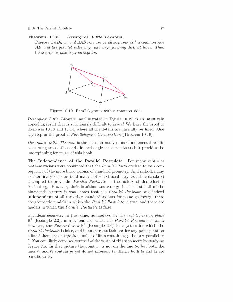
§I.10. The Parallel Postulate 77
Theorem 10.18. Desargues’ Little Theorem .Suppose �ABy1x1 and �ABy2x2 are parallelograms with a common sideAB and the parallel sides x1y1 and x2y2 forming distinct lines. Then�x1x2y2y1 is also a parallelogram.
A
x1
x2
y1
y2
B
Figure 10.19. Parallelograms with a common side.
Desargues’ Little Theorem, as illustrated in Figure 10.19, is an intuitivelyappealing result that is surprisingly difficult to prove! We leave the proof toExercises 10.13 and 10.14, where all the details are carefully outlined. Onekey step in the proof is Parallelogram Construction (Theorem 10.16).
Desargues’ Little Theorem is the basis for many of our fundamental resultsconcerning translation and directed angle measure. As such it provides theunderpinning for much of this book.
The Independence of the Parallel Postulate. For many centuriesmathematicians were convinced that the Parallel Postulate had to be a con-sequence of the more basic axioms of standard geometry. And indeed, manyextraordinary scholars (and many not-so-extraordinary would-be scholars)attempted to prove the Parallel Postulate — the history of this effort isfascinating. However, their intuition was wrong: in the first half of thenineteenth century it was shown that the Parallel Postulate was indeedindependent of all the other standard axioms for plane geometry: thereare geometric models in which the Parallel Postulate is true, and there aremodels in which the Parallel Postulate is false.
Euclidean geometry in the plane, as modeled by the real Cartesian planeR2 (Example 2.2), is a system for which the Parallel Postulate is valid.However, the Poincare disk P2 (Example 2.4) is a system for which theParallel Postulate is false, and in an extreme fashion: for any point p not ona line ℓ there are an infinite number of lines containing p that are parallel toℓ. You can likely convince yourself of the truth of this statement by studyingFigure 2.5. In that picture the point p1 is not on the line ℓ2, but both thelines ℓ3 and ℓ4 contain p1 yet do not intersect ℓ2. Hence both ℓ3 and ℓ4 areparallel to ℓ2.

78 Revision v2.0 , Chapter I, Foundations of Geometry in the Plane
However, it is not yet obvious that all of our earlier axioms are valid forP2. In particular, we have not specified the coordinate systems we use onlines (hence the distance function has not yet been specified), nor have weproduced an angle measure function. We will not go into these matters atthis time, but will simply state that definitions for all of these quantitiescan indeed be made so that the Poincare disk will satisfy all of our previousaxioms. The Poincare disk is a model for what is known as hyperbolicgeometry, an example of a non-Euclidean geometry since a negation ofthe Parallel Postulate is valid for the system. We will study such geometriesin Volume II of this text.
Exercises I.10
Exercise 10.1.
Let m1 and m2 be two distinct lines cut by a transversal ℓ. If ∠x and∠y are alternate interior angles and ∠y and ∠z are vertical angles, then∠x and ∠z are corresponding angles. Prove m1 and m2 are parallelif and only if a pair of corresponding angles are congruent.
Exercise 10.2.
Suppose m1 and m2 are parallel lines and ℓ a third line which intersectsm1 in a single point. Prove ℓ also intersects m2 in a single point andhence must be a transversal for m1 and m2 if these two lines are distinct.
Exercise 10.3.
(a) Prove the forward direction of Proposition 10.7:
If two lines m1 and m2 are parallel then any line ℓ perpendicularto m1 is also perpendicular to m2.
Hints: Assume m1 and m2 are parallel and take ℓ to be any lineperpendicular to m1 at a point p ∈ m1. You must show ℓ is perpen-dicular to m2. Since the case m1 = m2 is trivial you may assumem1 and m2 are disjoint. To show ℓ ⊥ m2 you must first show thatℓ actually intersects m2. This is Exercise 10.2.
(b) Prove the reverse direction of Proposition 10.7:
The two lines m1 and m2 will be parallel if whenever a line ℓ isperpendicular to m1, ℓ is also perpendicular to m2.
Hint: First show there does exist a line ℓ perpendicular to m1.Then, by our current assumption, ℓ is also perpendicular to m2.
(c) Give a second proof of the transitivity of parallelism (Theorem 10.6)based on Proposition 10.7.

§I.10. The Parallel Postulate 79
Exercise 10.4.
Suppose ℓ and ℓ′ are distinct parallel lines and a is a point on ℓ.
(a) Prove there exists a point a′ ∈ ℓ′ such that aa′ is perpendicular toℓ. Further prove a′ is unique and aa′ is also perpendicular to ℓ′.
(b) Prove that the number aa′ is independent of the choice of the pointa on ℓ, i.e., if b is any other point on ℓ and b′ is the correspondingpoint on ℓ′ such that bb′ is perpendicular to ℓ, then aa′ = bb′. Thisnumber is called the distance between the parallel lines ℓ and ℓ′.Does this result depend on the Parallel Postulate? Explain.
Exercise 10.5.
(a) Prove Proposition 10.8: Every Saccheri quadrilateral is a rectanglewhen the Parallel Postulate is assumed. Be sure to carefully pointout how your proof depends on the Parallel Postulate.Hint: In the Saccheri quadrilateral �abcd shown in Figure 9.12 youneed to show that ∠abc and ∠bcd are both right angles. Showingthe first of these angles is a right angle can be accomplished byverifying that △abc ∼= △cda.
(b) For this exercise let the Rectangle Hypothesis be the statement thatevery Saccheri quadrilateral is a rectangle. Without using the Par-allel Postulate or any result derived from the Parallel Postulate,prove that the Rectangle Hypothesis implies the Triangle Sum Hy-pothesis, i.e., that the sum of the measures of the interior angles ofany triangle equals 180◦.Hint: Modify the arguments of Exercise 9.3. In particular, in part(a) use Exercise 9.1 in place of Exercise 9.2; parts (b) and (c) requirelittle alteration.
(c) Show that the Parallel Postulate and the Rectangle Hypothesis areequivalent as described in Exercise 9.4. Hint: You will need theresult of Exercise 9.4.
Exercise 10.6.
(a) For any triangle △ABC prove that
AB ∼= BC if and only if the angle bisecting ray −→r for ∠B isparallel to the perpendicular bisector ℓ of AC.
If −→r and ℓ are indeed parallel, further show that −→r ⊂ ℓ.(b) Prove the following for any triangle △ABC:
If △ABC is a triangle for which AB 6= BC, then the anglebisecting ray −→r for ∠B intersects the perpendicular bisector ℓfor AC at a single point O.

80 Revision v2.0 , Chapter I, Foundations of Geometry in the Plane
Hints: This is a challenging exercise. Let m be the line containingthe angle bisecting ray −→r . From (a) ℓ and m intersect in a unique
point O. You must prove−→BO is the angle bisecting ray −→r for ∠B
(or equivalently, that the point O is interior to the angle ∠B).
Exercise 10.7.
(a) For any triangle, prove that the measure of an exterior angle equalsthe sum of the measures of the two remote interior angles.
Recall that circles were defined in Exercise 7.5.
(b) The Theorem of Thales. Suppose AB is a diameter of a circle C andC is a point on C other than A or B. Prove that ∠ACB is a rightangle. Hint: Suppose p is the center of the circle C. Analyze thetwo triangles △ApC and △BpC.
(c) Prove the converse of the Theorem of Thales: Suppose ∠ApB is aright angle. Then p is on the circle C with diameter AB. Hint :Let C be the midpoint of AB. Then analyze the angles of the twotriangles △ApC and △BpC.
(d) Challenge Exercise. Prove that the Theorem of Thales is equivalentto the Parallel Postulate as described in Exercises 9.4 and 10.5.
Exercise 10.8. The Inscribed Angle Theorem .
Let A, B, C be distinct points on a circle C with center P (Exercise 7.5).
intercepted
A
B
C
Parc
inscribedangle
centralangle
Figure 10.20. Inscribed angle, central angle, and intercepted arc.
The following objects are illustrated in Figure 10.20.
• ∠ABC is an inscribed angle of the circle C.• The portion of C which is interior to ∠ABC, along with the points
A and C, is the intercepted arc AC for ∠ABC.
• The intercepted arc for ∠ABC defines a central angle ∠cAPC, themeasure of which varies between 0 and 360◦. (The values between180◦ and 360◦ occur when the intercepted arc comprises more thanhalf of the circle.) The measure of this central angle is taken to bethe measure of the intercepted arc.

§I.10. The Parallel Postulate 81
In this exercise you will prove that the measure of an inscribed angle∠ABC is half the measure of its intercepted arc. The proof is done inthree steps, covering all possible locations for A, B, and C.
(a) First suppose BC is a diameter of the circle, as shown in the firstframe of Figure 10.21. You must show m∠2 = 2m∠1.
(b) Suppose BD is a diameter of the circle with A and C on oppositesides as shown in the second frame of Figure 10.21. You must showm∠4 = 2m∠3. Hint: Two applications of (a).
(c) Again suppose BD a diameter of the circle but this time with Aand C on the same side as shown in the third frame of Figure 10.21.You must show m∠6 = 2m∠5.
5 6
3 4
A
B CP
1 2
A
B
C
P
A
B
C
PD D
Figure 10.21. Cases for proving m∠ABC = 12 m∠cAPC = 1
2 m(AC).
Exercise 10.9.
Suppose A1, A2, B1, B2 are four points on a circle, ordered so that�A1A2B2B1 is a quadrilateral:
1
2
A1
A2
B2
B1
A1
A2
B2
B1
(a) Prove that the angles ∠1 = ∠B1A1B2 and ∠2 = ∠B1A2B2 arecongruent. This proves the following important property of circles:
Angles inscribed in the same arc of a circle are congruent.
(b) Show that the opposite interior angles in the inscribed quadrilateral�A1A2B2B1 are supplementary.
Exercise 10.10.
(a) Prove that a parallelogram is a convex quadrilateral (Definition 5.10).
(b) Prove Proposition 10.10c: The diagonals of a parallelogram bisecteach other. Hint: Recall Proposition 5.13.

82 Revision v2.0 , Chapter I, Foundations of Geometry in the Plane
(c) A rhombus is a parallelogram whose four sides are all congruent.Prove that the diagonals of any rhombus intersect at right angles.
(d) Prove a parallelogram vertex is in the interior of the opposite angle.
Exercise 10.11.
(a) Prove that a convex quadrilateral �abcd whose opposite sides arecongruent (i.e., ab ∼= cd and ad ∼= bc) is a parallelogram.
(b) Prove that every rectangle (Definition 9.11) is a parallelogram.
Exercise 10.12.
Suppose �ABy1x1 and �ABy2x2 are both parallelograms as shown inFigure 10.22. Prove x1x2
∼= y1y2 without the use of Desargues’ LittleTheorem! 12 Structure your proof in the following way.
A
x1
x2
y1
y2
B
C
Figure 10.22. Given two parallelograms, prove x1x2∼= y1y2.
(a) First consider the case where A, x1, and x2 are collinear.
The remaining steps consider when A, x1, and x2 are non-collinear.
(b) Show that x1 and y1 both lie on the same side of the line←→AB, and
similarly for x2 and y2.
(c) Assume x1, y1, x2, y2 all lie on the same side of←→AB, and let C
be a point on the line←→AB such that B is between A and C. Then
apply Exercise 5.5a to ∠x1AC and ∠x2AC, and use Exercise 10.1 toconclude ∠x1Ax2
∼= ∠y1By2. Show how this implies x1x2∼= y1y2,
the desired result.
(d) Finish the proof by showing x1x2∼= y1y2 when x1 and y1 lie on the
side of←→AB opposite to x2 and y2.
12It is also true that x1x2 and y1y2 are parallel, but this is surprisingly hard to prove. Inparticular, it requires Desargues’ Little Theorem (Theorem 10.18).

§I.10. The Parallel Postulate 83
Exercise 10.13. The Ray Separation Theorem.
This result will be needed for the proof of Desarges’ Little Theorem:
Suppose two parallel rays−−→a1b1 and
−−→a2b2 both lie on one side of a
line m which is not parallel to the rays. If ℓ is a line that separatesthe rays, then ℓ must be parallel to the rays.
Let m1 and m2 denote lines m1 =←→a1b1 and m2 =
←→a2b2, let m intersect
m1 and m2 at the points d1 and d2, respectively, and let n =←−→a1a2.
(a) Show that the rays−−→a1b1 and
−−→a2b2 are on the same side of n.
Hint: Suppose that the rays−−→a1b1 and
−−→a2b2 are on opposite sides of
n. Then show d1d2 intersects n at some point e. However, showthat e cannot equal a1 or a2 (easy), but neither can it lie betweena1 and a2, nor can it lie on the ray opposite −−→a1a2 (consider sides ofm1) or the ray opposite −−→a2a1 (consider sides of m2).
(b) Prove that ℓ intersects a1a2 at some point e. (Easy!)
(c) Suppose k is any line through e but unequal to n and not parallelto m1 and m2. Prove that k must intersect m1 and m2 at pointsc1 ∈ m1 and c2 ∈ m2 where c1 and c2 are on opposite sides of n.Hint: The line k intersects n at a point q. Show q must lie betweenc1 and c2 by proving that the other locations for q are impossible.
(d) Show ℓ must be parallel to m1 and m2, as desired. Hint: If ℓ is notparallel to m1 and m2, then use k = ℓ in (c) to contradict (a).
Exercise 10.14. Desargues’ Little Theorem.
Suppose �ABy1x1 and �ABy2x2 are both parallelograms with←−→x1y1 and←−→x2y2 distinct lines as shown in Figure 10.22. Prove that �x1x2y2y1 isalso a parallelogram. This is Desargues’ Little Theorem (Theorem 10.18).Structure your proof as follows.
(a) First show that the desired result will follow if you prove y1 andy2 lie on the same side of ←−→x1x2. Hint: Parallelogram Construction(Theorem 10.16).
In view of (a) we will now assume y1 and y2 do not lie on the same sideof ←−→x1x2 and work towards a contradiction.
(b) Show −−→x1y1 and −−→x2y2 are on opposite sides of the line ℓ =←−→x1x2.
(c) Consider the case where x1 and x2 are both on the same side of←→AB. By interchanging the labels of x1 and x2 if necessary, you canassume ∠BAx2 ≥ ∠BAx1. Prove the parallel rays −−→x1y1 and −−→x2y2
are then on the same side of m =←→Ax2. Hint: Show both −−→x1y1 and
−−→x2y2 must lie on the same side of m as−→AB.

84 Revision v2.0 , Chapter I, Foundations of Geometry in the Plane
(d) Consider the case where x1 and x2 are on opposite sides of←→AB.
As in (c), show that (by relabeling if necessary) you can arrange to
have the parallel rays −−→x1y1 and −−→x2y2 on the same side of m =←→Ax2.
(e) In all cases you now have (by relabeling if necessary) the parallelrays −−→x1y1 and −−→x2y2 separated by ℓ = ←−→x1x2 but on the same side of
m =←→Ax2. Conclude that this is impossible, and hence y1 and y2
must lie on the same side of x1x2, as desired. Hint: Exercise 10.13,the Ray Separation Theorem.
§I.11 Directed Angle Measure and Ray Translation
Global Rotational Direction. In §6 we defined the concept of directedangle measure at each point in the plane. We further observed that ateach point we had a choice of exactly two different directed angle measures,each one the negative of the other. Essentially, one measure gives a pos-itive sign to “clockwise” rotation while the other gives a positive sign to“counterclockwise” rotation. However, we also noted a difficulty: there isno good definition for clockwise versus counterclockwise. They are simplythe “opposites” of each other.
And herein lies a seriously thorny problem. We wish to consistently choosea directed angle measure at all points of the plane, say counterclockwisedirected angle measure at every point. But though we are quite sure whatthis means intuitively, as just observed, there is no simple, rigorous way todefine “counterclockwise” rotation at a point.
The intuitive meaning of “counterclockwise” suggests a solution. “Counter-clockwise” means the opposite direction to a clock. In other words, rotationsare classified by comparison against a clock. So pick some object with a fixedrotational direction (like a clock), arbitrarily designate its rotational direc-tion as “clockwise,” and then classify all other rotations as clockwise orcounterclockwise via comparison with the fixed, “standard” clock.
However, there is still a difficulty. The comparison process assumes we cantake the “standard” clock and move it to any point p in the plane andcompare its rotation with any other rotation at p. However, how do weknow this process will be consistent, i.e., might the process of “moving theclock around the plane” actually change the rotational direction of the clock?
There are geometric spaces in which this actually happens! Consider theMobius band. To construct a Mobius band take a rectangular strip ofpaper which is much longer than it is wide. If you wrap the ends of the striparound and glue them together in the ordinary fashion, you obtain the side ofa cylinder, as shown in the left half of Figure 11.1. However, if before gluing

§I.11. Directed Angle Measure and Ray Translation 85
the ends together you give the strip a half-twist, i.e., a rotation of 180◦, youobtain a Mobius band. This is shown in the right half of Figure 11.1.
A Mobius band has the curious property of being one-sided. To see this,start with a dot anywhere on the band and move the dot along the band asthough you were going around a cylinder. When you go all the way around,you will find your dot on the “other side” of the surface! In this way theMobius band has only one side.
Figure 11.1. A cylinder compared with a Mobius band.
However, suppose you repeat the movement of the previous paragraph, butthis time not with a simple dot but with a “clockwise angle” of, say, 30◦.As with the dot, when you move the angle around the band, you will endup on the “other side” of the surface. However, an idealized surface has nothickness, so that any collection of points on the surface really exists on bothsides of the surface simultaneously! So our angle can be considered as anobject on both sides of the band, including the side of the band on which theangle started. However, as can be seen in Figure 11.2, the rotation directionof the angle has changed from counterclockwise to clockwise! So translating arotation on a Mobius band will interchange clockwise and counterclockwise.
Figure 11.2. Going around a Mobius band reverses rotational direction.
We should not expect that moving an angle around in the Euclidean planeE could produce such a reversal of rotational direction. However, this beliefneeds to be verified from our axioms for the Euclidean plane.
The way we handle all the problems in this section is to show that directedangle measure assignments can be made at each point in the plane that aretranslationally invariant, meaning that “parallel translation” of a directed

86 Revision v2.0 , Chapter I, Foundations of Geometry in the Plane
angle (i.e., moving it “without rotation”) from one point to another willnot change its directed angle measure. Hence the Euclidean plane does notbehave like a Mobius band. No new axioms need be added to our collection,i.e., translationally invariant notions of clockwise and counterclockwise arealready inherent in the Euclidean plane.
Translational Invariance. Choose a point a0 in the plane. According toProposition 6.16, two directed angle measures exist at a0. Choose one ofthese measures, denoted by m, and interpret positive values of m to indicatecounterclockwise rotation and negative values to indicate clockwise rotation.
We wish to choose a “counterclockwise” rotational direction at each pointof the plane which is “consistent” with the choice made at a0. Followingour analogy of moving a clock around from point to point in the plane, theconsistency we desire is translational invariance. To develop this concept,we first consider the translation of rays, then of directed angles.
Ray Translation. Though the concept of ray translation is intuitively sim-ple — “move” a ray in the plane without rotating it or changing its length byexpansion or contraction — capturing this concept in a formal definition andrigorously establishing its properties is far deeper than you would imagine.The key foundational principle is Desargues’ Little Theorem. However, acareful development of ray translation yields a rich harvest: the fundamen-tal properties of directed angle measure, rotations, and translations. Wewould have no book without these concepts.
b
a
b
ℓ
a
ℓ
a
b
a
b
ℓℓ =
Figure 11.3. In each picture−→ab and
−→a′b′ are translates of each other.
Definition 11.4.
Two rays−→ab and
−→a′b′ are translates of each other if either
(1) the lines ℓ =←→ab and ℓ′ =
←→a′b′ are distinct parallel lines such that b
and b′ lie on the same side of←→aa′ or
(2) one of the rays−→ab and
−→a′b′ is a subset of the other.
The two types of ray translates are shown in Figure 11.3.

§I.11. Directed Angle Measure and Ray Translation 87
The properties we need of ray translation are intuitive and unsurprising:
given a ray−−→a1b1, (1) there exists a unique translate of this ray to any other
point a2 in the plane and (2) if you translate−−→a1b1 to
−−→a2b2 and then translate
this new ray to−−→a3b3, the result is the same as translating
−−→a1b1 to
−−→a3b3. These
properties are given below in Proposition 11.5 and Theorem 11.6.
Proposition 11.5.
Given a ray−→ab and any point a′, there exists exactly one ray
−→a′b′ with
initial point a′ that is a translate of−→ab.
Proof. Case (1). Suppose a′ is not on the line ℓ =←→ab . To prove the existence
of a translate ray−→a′b′, note that by Parallelogram Existence (Theorem 10.14)
there exists a unique point b′ such that �abb′a′ is a parallelogram. The ray−→a′b′ is easily seen to be a translate of
−→ab.
To prove−→a′b′ is the unique translate of
−→ab starting at a′, suppose
−−→a′b′′ is
another such ray. By Axiom PP, the Parallel Postulate, there exists only
one line ℓ′ through a′ which is parallel to ℓ. Thus the two rays−→a′b′ and
−−→a′b′′
both lie on this line, and thus−−→a′b′′ equals
−→a′b′ or its opposite. However, the
ray opposite to−→a′b′ is not a translate of
−→ab and thus
−−→a′b′′ must equal
−→a′b′, as
desired. This proves the desired uniqueness in case (1).
Case (2). Suppose a′ is on the line ℓ =←→ab . Using the Ruler Placement
Theorem (Proposition 3.6), choose a coordinate system χ : ℓ → R suchthat χ(a) = 0 and χ(b) > 0. In addition, choose a point b′ on ℓ such thatχ(b′) > χ(a′). Then, as in Exercise 4.4, we obtain
−→ab = {c ∈ ℓ | 0 ≤ χ(c)},−→a′b′ = {c ∈ ℓ | χ(a′) ≤ χ(c)}.
Thus, if χ(a′) ≥ 0, then−→a′b′ ⊂ −→ab, but if χ(a′) < 0, then
−→ab ⊂ −→a′b′. In either
case,−→a′b′ is a translate of
−→ab, as desired. Uniqueness of
−→a′b′ is verified as
follows. Since a′ is on the line ℓ =←→ab , any translate of
−→ab which starts at
a′ will lie on ℓ. But then there are only two possibilities for the translate:−→a′b′ or its opposite. But the opposite ray, which consists of all the points c
on the line ℓ with χ(c) ≤ χ(a′), cannot contain or be contained in−→ab. Thus
the assumed translate ray must be−→a′b′, proving the desired uniqueness. �
In view of Proposition 11.5 we see that any ray−→ab starting at the point a
can be uniquely translated to any other point a′, by which we mean the ray−→ab has a unique translate ray
−→a′b′ starting at a′. However, we need to know
more. In particular, we need to know that translation of rays is transitive.This is a much deeper result than you would ever suspect!

88 Revision v2.0 , Chapter I, Foundations of Geometry in the Plane
Theorem 11.6. Transitivity of Ray Translation.
Translation of rays is transitive. Thus if−−→a1b1 translates to
−−→a2b2 and−−→
a2b2 translates to−−→a3b3, then
−−→a1b1 translates to
−−→a3b3.
Proof. For convenience we assume the points b1, b2, b3 have been picked sothat the distances a1b1, a2b2, a3b3 are all equal. This can always be doneby Segment Construction (Proposition 4.10). Since parallelism is transitive
(Theorem 10.6) the lines ℓ1 =←→a1b1 and ℓ3 =
←→a3b3 are parallel to each other
since both are parallel to ℓ2 =←→a2b2.
Now assume the generic case where all three lines ℓ1, ℓ2, ℓ3 are distinct. To
show−−→a1b1 translates to
−−→a3b3, we have only to show that b1 and b3 lie on the
same side of the line m =←−→a1a3. See Figure 11.7.
m
ℓ1
ℓ2 ℓ3
a1
b1
a2
b2
a3
b3
Figure 11.7. Need to verify b1 and b3 on the same side of m =←−→a1a3.
However, we know that the two line segments a1b1 and a2b2 are parallel,have the same length, and have the endpoints b1 and b2 on the same sideof the line m3 = ←−→a1a2. But these are the exact conditions needed in Par-allelogram Construction (Theorem 10.16) to conclude that �a1b1b2a2 is aparallelogram. The same argument shows that �a2b2b3a3 is a parallelogram.Thus, since the three lines ℓ1, ℓ2, and ℓ3 are all distinct, Desargues’ LittleTheorem (Theorem 10.18) gives that �a1b1b3a3 is also a parallelogram,13
proving that the ray−−→a3b3 is indeed a translate of the ray
−−→a1b1.
The various “degenerate” cases, where two or more of the lines ℓ1, ℓ2, ℓ3 arethe same, will be considered in Exercise 11.1. Most are not trivial. �
The rest of this section may be skipped by readers needing onlyan intuitive treatment of clockwise/counterclockwise rotation,
ray translation, and directed angle measure.
13Recall that the difficult part of the proof of Desargues’ Little Theorem is that b1 and b3are indeed on the same side of the line ←−→a1a3. Simple statements are sometimes the most difficult!

§I.11. Directed Angle Measure and Ray Translation 89
Directed Angle Translation. We translate directed angles by translatingeach of the two rays of the angle. Ultimately this will allow us to choose a“counterclockwise” directed angle measure at one point a0 and then trans-late this choice to all other points in the plane. However, before we cancarry out this plan, we need some properties of directed angle translation.
Definition 11.8.
Two directed angles ∡abc and ∡a′b′c′ are said to be translates of eachother, denoted by ∡abc ≡τ ∡a′b′c′, if
• −→ba and−→b′a′ are translates of each other and
• −→bc and−→b′c′ are translates of each other.
Proposition 11.9.Given a directed angle ∡abc and any point b′, there exists exactly onedirected angle ∡a′b′c′ with vertex b′ that is a translate of ∡abc.
Proof. This is a quick corollary of Proposition 11.5: simply apply that result
to each ray−→ba and
−→bc . �
Proposition 11.10.Translation of directed angles is an equivalence relation, i.e., the rela-tionship ≡τ is reflexive, symmetry, and transitive.
Proof. To prove that ≡τ is reflexive means verifying any directed angle is atranslate of itself. This is trivial from the definition of translation.
To prove that ≡τ is symmetric means showing ∡A′ ≡τ ∡A whenever wehave ∡A ≡τ ∡A′. This is easy to verify from the definition of directed angle
translation since if−→ab is a translate of
−→a′b′, then
−→a′b′ is a translate of
−→ab.
Transitivity for directed angle translation is a corollary of the transitivity ofray translation as given in Theorem 11.6. For suppose ∡abc ≡τ ∡a′b′c′ and
∡a′b′c′ ≡τ ∡a′′b′′c′′. Then rays−→ba and
−→b′a′ are translates of each other and
rays−→b′a′ and
−−→b′′a′′ are translates of each other. Thus Theorem 11.6 gives
that−→ba and
−−→b′′a′′ are translates of each other. Similarly rays
−→bc and
−→b′c′′ are
translates of each other, proving ∡abc ≡τ ∡a′′b′′c′′, as desired. �
Recall that a trivial directed angle is a directed angle made from two iden-tical rays, so that any directed angle measure will assign 0 (mod 360) to thisangle. A straight directed angle is a directed angle made from two oppositerays, so that any directed angle measure will assign 180◦ (mod 360) to sucha directed angle. It is quite natural to expect directed angle translation topreserve such angles; this is the content of the next proposition. Its proof isquite easy and is left to Exercise 11.3.

90 Revision v2.0 , Chapter I, Foundations of Geometry in the Plane
Proposition 11.11.A translate of a trivial directed angle is another trivial directed angle.A translate of a straight directed angle is another straight directed angle.
The next proposition handles translates of non-trivial and non-straight di-rected angles. It too is a highly intuitive result: translation does not change(ordinary) angle measure, so that directed angles which are translates ofeach other are congruent as (ordinary) angles.
Proposition 11.12.Non-trivial, non-straight directed angles that are translates of each otherare congruent, i.e., they have the same (ordinary) angle measure.
Proof. Let ∡abc and ∡a′b′c′ be translates of each other where, for conve-nience, a, c, a′, and c′ are chosen so that ba = b′a′ and bc = b′c′. We first
consider the generic situation:←→ba and
←→b′a′ are distinct parallel lines and
←→bc
and←→b′c′ are distinct parallel lines. If necessary, adjust the length ba = b′a′
so that lines←→aa′ and
←→cc′ are distinct parallel lines. See Figure 11.13.
a
b
c
a
b
c
Figure 11.13. ∡abc and ∡a′b′c′ are translates of each other.
With these choices the definition of ray translation along with Parallelo-gram Construction (Theorem 10.16) show �b′baa′ and �b′bcc′ to be paral-lelograms. Then Desargues’ Little Theorem (Theorem 10.18) shows �aa′c′cto be a parallelogram. In particular, ac = a′c′. Therefore triangles △abcand △a′b′c′ are congruent by SSS (Theorem 7.11). Thus ∠abc ∼= ∠a′b′c′.
The degenerate cases,←→ba =
←→b′a′ and/or
←→bc =
←→b′c′, are in Exercise 11.2. �
Translationally Invariant Directed Angle Measure. As shown inPropositions 11.11 and 11.12, translation of a directed angle does not changeits ordinary angle measure. However, we would also like its directed anglemeasure not to change. For this to be true, we must make consistent choicesof directed angle measure at each point in the plane. So fix a point a0, pickone of the two choices of directed angle measure at that point, and then“translate” that choice to all other points by translation of directed angles.The details follow....

§I.11. Directed Angle Measure and Ray Translation 91
Definition 11.14.
A directed angle measure m defined at every point is translationallyinvariant if the measure is unchanged under directed angle translation:
if ∡A and ∡A′ are translates of each other, then m∡A = m∡A′.
We finally come to the big result: there exist exactly two translationallyinvariant directed angle measures in the plane. These two measures justifyour intuitive notions of clockwise and counterclockwise. We interpret one ofthe directed angle measures — denote it as m+ — as measuring directedangles using a counterclockwise orientation and the other — denote it asm− — as using a clockwise orientation. Thus, under m+, a positive di-rected angle measure indicates a counterclockwise turn from the initial rayto the terminal ray, while a negative value indicates a clockwise turn (alsocalled a negative counterclockwise turn). For m− the roles of clockwise andcounterclockwise are reversed.
Theorem 11.15.Exactly two translationally invariant directed angle measures exist in theEuclidean plane E. Each measure is the negative of the other.
Proof. We first show that there can be at most two translationally invari-ant directed angle measures on the plane. We already know from Propo-sition 6.16 that at a given point a0 there are precisely two directed anglemeasures. However, the assumed translation invariance of the angle measureshows that when the directed angle measure values are established at onepoint a0, then they are immediately determined at every other point a′ inthe plane. To see this, take any directed angle ∡A′ with vertex at a′ and let∡A be the translate of ∡A′ with vertex a0. By our construction the directedangle measure of ∡A′ must equal the directed angle measure of ∡A. Henceestablishing the values of the direct angle measure at a0 also determines thevalues at a′. Since there are only two choices for the directed angle measureat a0, this proves that there can be at most two translationally invariantdirected angle measures in the plane.
To show the existence of the two translationally invariant directed anglemeasures, pick a point a0 in the plane. We know from Proposition 6.16 thatthere exist precisely two directed angle measures at a0. Pick one of thesedirected angle measures at a0, denoting it by m0.
Let a′ be any point in the plane and ∡A′ any directed angle with vertex a′.Then, letting ∡A0 denote the translate of ∡A′ to the vertex a0 as shown inFigure 11.17, define the directed angle measure of ∡A′ to be
m∡A′ = m0 ∡A0. (11.16)

92 Revision v2.0 , Chapter I, Foundations of Geometry in the Plane
∡A0a0
∡Aa
Figure 11.17. m∡A′ is defined to be m0 ∡A0.
To finish the proof requires showing that (11.16) definesm to be a translationinvariant directed angle measure. Verifying that at each point a′ we obtaina directed angle measure is straightforward. However, as we will see, thefact that m is translationally invariant is a deeper result.
We first verify that m, as defined by (11.16), is a directed angle measure ata′. We do so by checking the four conditions of Definition 6.15:
(1) Suppose ∡A′ is trivial, i.e., it is one ray starting at a′. Then ∡A0, thetranslate of ∡A′ to vertex a0, is also trivial by Proposition 11.11. Hence
m∡A′ = m0∡A0 = 0 mod 360.
(2) Suppose ∡A′ is a straight angle, i.e., it is composed of two opposite raysstarting at a′. Then ∡A0, the translate of ∡A′ to vertex a0, is also astraight angle by Proposition 11.11. Hence
m∡A′ = m0∡A0 = 180◦ mod 360.
(3) Suppose ∡A′ is a directed angle at a′ that is neither trivial nor straight.If θ′ is that value of m∡A′ such that −180◦ < θ′ < 180◦, then we wishto show |θ′| = m∠A′, i.e., that |θ′| is the measure of the (ordinary)angle ∠A′. By Proposition 11.12, ∡A′ is the translate of a directedangle ∡A0 with vertex at a0 that is neither trivial nor straight, and the(ordinary) angles ∠A′ and ∠A0 are congruent. Moreover, by definitionof m, m∡A′ = m0∡A0. Hence θ′ is that value of m0∡A0 such that−180◦ < θ′ < 180◦. Thus
|θ′| = m∠A0 from (3) of Definition 6.15, m0 a directed angle measure,
= m∠A′ since ∠A0∼= ∠A′. This is the desired result.
(4) Suppose b′, c′, d′ are any three points other than a′, and let−→a0b,
−→a0c,−→a0d be the translates to a0 of the rays
−→a′b′,
−→a′c′,
−→a′d′, respectively. Then
m∡b′a′d′ = m0∡ba0d by definition of m at a′,
= m0∡ba0c+m0∡ca0d by condition (4) for m0 at a0,
= m∡b′a′c′ +m∡c′a′d′ by definition of m at a′.

§I.11. Directed Angle Measure and Ray Translation 93
Finally, we must verify that m is translationally invariant. So consider adirected angle ∡A′ at a point a′ and its translate ∡A′′ to a point a′′ asshown in Figure 11.18. Thus ∡A′ ≡τ ∡A′′. We must show
m∡A′ = m∡A′′.
To do so, recall that m∡A′ is defined by
m∡A′ = m0 ∡A0,
where ∡A0 is the translate of ∡A′ to the point a0 as shown to the right.Thus ∡A′ ≡τ ∡A0. However, since directed angle translation is transitiveby Proposition 11.10, ∡A′′ ≡τ ∡A0. Thus
m∡A′′ = m0∡A0 = m∡A′,
proving m∡A′ = m∡A′′, as desired. This finishes the proof that m, asconstructed above, is a translationally invariant directed angle measure. �
a0 ∡A0
a ∡A
∡Aa
Figure 11.18. Proving that m is translationally invariant.
Exercises I.11
Exercise 11.1.
In this exercise you complete the proof Theorem 11.6, the transitivity of
ray translation, by verifying the various degenerate cases. Assume−−→a1b1
translates to−−→a2b2,
−−→a2b2 translates to
−−→a3b3, and (for convenience) b1, b2,
and b3 are chosen so that a1b1 = a2b2 = a3b3. You need to prove−−→a1b1
translates to−−→a3b3. As in the theorem define lines ℓ1 =
←→a1b1, ℓ2 =
←→a2b2,
and ℓ3 =←→a3b3. The proof for the generic case, when the three lines are
all distinct, was given in the text. Now handle the other cases:
(a) Assume ℓ1 and ℓ2 are distinct but a3 lies on ℓ2. Then ℓ2 = ℓ3.Proof sketch: If a2 = a3, then b2 = b3 and the desired result follows.
If a2 6= a3, then either−−→a2b2 contains
−−→a3b3 or
−−→a3b3 contains
−−→a2b2.
Assume the second case; the first case is similar. Then a2 is between

94 Revision v2.0 , Chapter I, Foundations of Geometry in the Plane
a3 and b2, and the three points a2, b2, b3 all lie on the same sideof ←−→a1a3 (why?). You must show b1 lies on this same side of ←−→a1a3.Suppose not. Then show the line segment a1a3 must intersect the
line m =←→b1b2, showing a1 and a3 to be on opposite sides of m. But
a2 and a3 must lie on the same side of m (why?), which means a1
and a2 must lie on opposite sides of m. But this is not possible(why?). Use this to finish the proof.
(b) Assume ℓ1 and ℓ2 are distinct but a3 lies on ℓ1. Then ℓ1 = ℓ3.Hints: There are two non-trivial cases to consider: b1, a3 on thesame side or on opposite sides of a1. Consider the same side case:
you need to show−−→a3b3 ⊆
−−→a1b1, which will be true if a3 is between
a1 and b3. This is equivalent to showing a1 and b3 are on oppositesides of m3 = ←−→a2a3. To prove this, first show b1, b2, a3 all lieon the same side of m1 = ←−→a1a2. However, �a1a2b2a3 is a convexquadrilateral (Definition 5.10) and so the diagonal line segmentsintersect by Proposition 5.13. Use this to show a1 and b3 are onopposite sides of m3, as desired. Then handle the case where b1 anda3 are on opposite sides of a1 . . . .
(c) Assume ℓ1 = ℓ2 but a3 is not on this line. Hint: A variant of (a).
(d) Assume ℓ1 = ℓ2 and a3 is on this line. Then ℓ1 = ℓ2 = ℓ3.Hint: Use a coordinate system on the line as done in Exercise 4.4.
Exercise 11.2.
Proposition 11.12 states that if ∡abc and ∡a′b′c′ are translates of eachother, then ∠abc ∼= ∠a′b′c′. The proof given in the text covered the
generic case, i.e., when←→ba and
←→b′a′ are distinct parallel lines and
←→bc
and←→b′c′ are distinct parallel lines. Complete the proof by handling the
degenerate cases when←→ba =
←→b′a′ and/or
←→bc =
←→b′c′.
Exercise 11.3.
Prove Proposition 11.11: A translate of a trivial directed angle is anothertrivial directed angle. A translate of a straight directed angle is anotherstraight directed angle.
§I.12 Similarity
Recall the definition for similar triangles:
Definition 12.1. Triangle Similarity.
(a) A similarity between two triangles, written△abc ∼ △ABC, meansthat the ratios of corresponding side lengths are equal and corre-sponding angles are congruent, i.e.,
AB
ab=BC
bc=AC
acand ∠a ∼= ∠A, ∠b ∼= ∠B, ∠c ∼= ∠C.

§I.12. Similarity 95
(b) Two triangles are similar if there exists a similarity between them.
A
B
C
a
b
c
Figure 12.2. △abc and △ABC are similar via abc↔ ABC.
It is a well-known theorem of geometry (Angle-Angle-Angle, or AAA) thattwo triangles are similar if and only if the three angles of the first triangleare congruent to the three angles of the second, as shown in Figure 12.3.In other words, the angle conditions for similarity are enough to imply thetruth of the ratio conditions for the sides.
A
B
C
a
b
c
α
β
γ
α
β
γ
Figure 12.3. Two similar triangles showing the equal angles.
However, deriving this theorem from our previously established results ismore difficult than initially expected: the proof requires a non-trivial pas-sage from the rational numbers to the real numbers. We isolate this difficultpassage in the Similarity Theorem and then use this result to prove AAA.Although AAA is the result of most immediate interest, the Similarity The-orem will play a major role in Chapter IV, Similarities in the Plane.
Theorem 12.4. The Similarity Theorem.Let ℓ, m be lines not containing the point p. Suppose −→r1 , −→r2 are distinctrays from p such that −→r1 intersects ℓ and m at x1, y1, respectively, and−→r2 intersects ℓ and m at x2, y2, respectively. Then the ratios
p
y2
y1
x1
x2
mℓ
¡→r1
¡→r2
py1
px1and
py2
px2
are equal if and only if the lines ℓ andm are parallel, in which case both of theratios equal
y1y2
x1x2.
Proof . To save time, you may decide to skip the proof—it is not trivial.Hence we place it as optional reading at the end of the section. �

96 Revision v2.0 , Chapter I, Foundations of Geometry in the Plane
Here is the most common method for verifying triangle similarity.
Theorem 12.5. AAA (Angle-Angle-Angle) Similarity .Two triangles are similar if and only if the three angles of the firsttriangle are congruent to the three angles of the second.
Proof. Suppose△ABC and △abc have congruent corresponding angles, i.e.,
m∠BAC = m∠bac = α,
m∠CBA = m∠cba = β,
m∠ACB = m∠acb = γ.
Using Proposition 4.10, Segment Construction, let b′ be that point on the
ray−→ab such that ab′ ∼= AB, and let c′ be that point on the ray −→ac such that
ac′ ∼= AC (see Figure 12.6).
A
B
C
a
b
c
α
β
γ
α
β
γ
b
c
Figure 12.6. △ABC and △abc have congruent corresponding angles.
Then, since m∠b′ac′ = α = m∠BAC, SAS proves △ABC and △ab′c′ are
congruent. Thus m∠c′b′a = m∠CBA = β. This shows that the lines←→b′c′
and←→bc are parallel since they have a congruent pair of corresponding angles
(Exercise 10.1). Hence, from the Similarity Theorem we concludeab
ab′=ac
ac′=
bc
b′c′.
Since △ABC and △ab′c′ are congruent, our equalities can be rewritten asab
AB=
ac
AC=
bc
BC,
verifying △ABC and △abc are similar. �
Actually, we have only to check two pairs of angles to verify similarity:
Corollary 12.7. AA (Angle-Angle) Similarity .Two triangles are similar if and only if two of the three angles of thefirst triangle are congruent to two of the three angles of the second.
Proof. AAA (Theorem 12.5) combined with the fact that the measures ofthe angles of any triangle add to 180◦ (Theorem 10.3). �

§I.12. Similarity 97
We can now state and prove what is perhaps the most famous theorem inall of Euclidean geometry: the Pythagorean Theorem. The proof we giveis based on similarity of triangles via the use of AAA. We will give otherproofs, based on area, in Chapter IX.
Recall that a right triangle is any triangle with a right angle. The hy-potenuse is the side of the triangle opposite the right angle.
Theorem 12.8. The Pythagorean Theorem .
A
a
B
Cb
c
In any right triangle, the square of thelength c of the hypotenuse is equal tothe sum of the squares of the lengths aand b of the other two sides. Thus
c2 = a2 + b2.
Proof. Let D be the point on the line←→AB such that CD is perpendicular to←→
AB. Since m∠ADC = 90◦, m∠ACD is less than 90◦ since the measures ofall the angles in △ACD sum to 180◦ by Theorem 10.3. Hence D is in theinterior of angle ∠ACB by Exercise 6.4, therefore falling on the line segmentAB between A and B.
Let α = m∠A and β = m∠B. Since the sum of the measures of the anglesof the right triangle △ABC equals 180◦, we obtain α + β = 90◦. However,this equality implies m∠ACD = β and m∠BCD = α:
A
a
B
Cb
D
α
βc1
c2
β
α
Hence AAA shows we have similar triangles △CBD ∼ △ABC ∼ △ACD:
β
α
ac1
B
CD
C
D A
β
α
b
c2A
a
B
C b
D
α
β
β
α
c = c1 + c2
The first similarity implies
c1a
=a
c, which gives c1 =
a2
c.

98 Revision v2.0 , Chapter I, Foundations of Geometry in the Plane
The second similarity implies
c2b
=b
c, which gives c2 =
b2
c.
Hence c = c1 + c2 =a2
c+b2
c, which yields c2 = a2 + b2. �
Diagonals of a Parallelogram. There is a useful generalization of thePythagorean Theorem to parallelograms. Its proof is left to Exercise 12.5.
Proposition 12.9.
Suppose �ABCD is a parallelogram with side lengths a and b and diag-onal lengths d1 and d2. Then
2(a2 + b2) = d21 + d2
2.
The Trigonometric Functions. Our results on triangle similarity areneeded to justify the usual geometric definitions of the trigonometric func-tions. We illustrate this procedure with the sine function.
Given a right triangle △ABC with right angle at ∠C, the sine of angle ∠Ais defined to be BC/AB, i.e., the length of the “opposite” side divided bythe length of the hypotenuse.
A
B
Cθ
A major property of the sine of an angle ∠Ais that it should depend only on the angularmeasure of ∠A, i.e., only on the value
θ = m∠A.
This property justifies the customary nota-tion of sin θ for the sine of any angle whosemeasure is θ.
To prove our claimed property, suppose △ABC and △A′B′C ′ are two righttriangles with right angles ∠C and ∠C ′, respectively, and m∠A = m∠A′:
θA
B
Cθ
A C
B
We wish to show that the sine of ∠A equals the sine of ∠A′, i.e.,
BC/AB = B′C ′/A′B′.

§I.12. Similarity 99
However, m∠A = m∠A′ by assumption, and m∠C = m∠C ′ since all rightangles have measure 90◦. Thus AA (Corollary 12.7) shows that the twotriangles △ABC and △A′B′C ′ are similar. Hence
BC/B′C ′ = AB/A′B′.
This proves BC/AB = B′C ′/A′B′, so the sine of ∠A does equal the sine of∠A′, as desired. Hence the sine of an angle depends only on the measure ofthe angle.
Justifications for the usual geometric definitions of the other trigonometricfunctions are identical to the one just given for the sine — see Exercises 12.8and 12.9.
Proof of the Similarity Theorem (Optional). The proof of the Simi-larity Theorem, based on our previously established axioms and theorems,is rarely given in elementary geometry courses as it involves an intricate,technically complicated argument proceeding from integer ratios to rationalratios and finally to real number ratios. To save time, you may simply decideto accept the truth of the Similarity Theorem and thus skip the followingproof. However, the proof utilizes several beautiful arguments and illus-trates the central importance of the real number system in our developmentof geometry.
Our proof of the Similarity Theorem begins with establishing a slightly re-duced version of the result: the Basic Similarity Principle. The full theoremcan then be deduced from this principle.
Theorem 12.10. The Basic Similarity Principle.
Let ℓ and m be parallel lines with ℓ not containing the point p. SupposeL1 and L2 are two lines containing p such that L1 intersects ℓ and mat x1, y1, respectively, and L2 intersects ℓ and m at x2, y2, respectively.Then the ratios
p
y2
y1
x1
x2
mℓ
L1
L2
py1
px1and
py2
px2
are equal. In particular, this ratio δ de-pends only on the choices of p, ℓ, and m,not on the choice of the line L through p.
Proof. If the parallel lines ℓ and m are equal, then the claims in the theoremare trivially true (the ratios are all 1). We thus assume that ℓ and m aredistinct parallel lines.
There are various cases to consider, depending on the placement of the pointp relative to the lines ℓ and m. The most trivial case is when p lies on theline m for then y1 = y2 = p and the ratios in the theorem are equal (since

100 Revision v2.0 , Chapter I, Foundations of Geometry in the Plane
they are both zero), as desired. Now consider the case when the point p isnot between the two lines m and ℓ (the case where p is between the two linesis treated similarly and is left to the reader). By interchanging the labels ofm and ℓ if necessary, we may assume that the point p and the line m are onopposite sides of the line ℓ, as shown in the diagram with Theorem 12.10.
The difficulty in the proof arises from the possible irrationality of the ratioδ. The technique of the following proof is to verify the theorem first forδ = 2, then for δ any integer ≥ 1, then for δ any rational number ≥ 1, thenfinally for δ any irrational number ≥ 1.
p
y2
y1
x1
x2
mℓ
δ = = 2py1px1
Figure 12.11. Setup for the Basic Similarity Principle when δ = 2.
So suppose p, ℓ, m, x1, y1, x2, and y2 are as in the hypothesis of the theorem.We first assume the ratio δ of py1 to px1 equals 2 as shown in Figure 12.11.This is equivalent to x1 being the midpoint of py1. We need to show thatthe ratio of py2 to px2 also equals 2. This means showing that x2 is betweenp and y2 and that px2 = x2y2.
The point x2 lies between p and y2 since ℓ and m are parallel lines.14 Hencewe need only show that px2 = x2y2. To do so, let y0 be that point on mbetween y1 and y2 such that x1y0 is parallel to py2. We will then show twofacts (see Figure 12.12):
(1) triangles △px1x2 and △x1y1y0 are congruent, so px2 = x1y0,
(2) the quadrilateral �x1y0y2x2 is a parallelogram; hence x1y0 = x2y2
from Proposition 10.10b.
These two facts give px2 = x2y2, as needed for the case δ = 2.
δ = = 2py1px1
py2
y1
x1
x2
y0
Figure 12.12. Two congruent triangles and a parallelogram.
14Since p lies on the side of ℓ not containing m, p and y1 are on opposite sides of ℓ, andhence x1 must lie between p and y1. However, since m is parallel to ℓ, the segment y1y2 remainson the same side of ℓ. Therefore p and y2 will be on opposite sides of ℓ, proving that x2 is betweenp and y2, as desired.

§I.12. Similarity 101
To prove (1), that △px1x2∼= △x1y1y0, we employ ASA (Theorem 7.8):
Angle: px2 is parallel to x1y0, so ∠x1px2∼= ∠y1x1y0 by Exercise 10.1.
Side: px1 = x1y1 by the assumption that δ = 2.
Angle: x1x2 is parallel to y1y0, so ∠px1x2∼= ∠x1y1y0 by Exercise 10.1.
To prove (2), that �x1y0y2x2 is a parallelogram, we have only to observethat each pair of opposite sides of the quadrilateral are comprised of parallellines. This proves the Basic Similarity Principle when the ratio δ equals 2.
Now suppose the ratio δ of py1 to px1 equals n, a positive integer. Thenselect those n−1 points which divide the line segment py1 into n equal pieces(such points exist as a consequence of the coordinate system on L1 =←→py1).The first of these segments will be px1 (see Figure 12.13).
p
y2
y1
x1
x2
δ = n
(n = 5 is shown)
Figure 12.13. Analyzing the case δ = n, an integer.
From each of the points just selected in py1 construct two lines: one parallelto py2 and the other parallel to y1y2. In this way the line segment py2 isitself divided up into n pieces, the first of which is px2 (see Figure 12.14).We must show that all these new line segments in py2 are the same length.When this is done, we will have that py2 = n px2, the desired relationshipbetween these two distances.
p
y2
y1
x1
x2
δ = n
(n = 5 is shown)
Figure 12.14. Subdivisions for the case δ = n, an integer.
Along the line segment py1 we now have n − 1 small overlapping triangleslike those considered in the previous case where δ = 2. One such triangle isshown in yellow in Figure 12.15.

102 Revision v2.0 , Chapter I, Foundations of Geometry in the Plane
p
y2
y1
x1
x2
δ = n
(n = 5 is shown)
Figure 12.15. Any two adjacent line segments in py2 are of equal length.
From the previous case of δ = 2 we see that the two line segments comprisingthe base of the small yellow triangle in Figure 12.15 (parallel to py2) are ofequal length. Moreover, each of these line segments is the top side of aparallelogram (shaded in blue and red) whose opposite side is one of the linesegments of py2 constructed above. Hence the two line segments in py2 sopicked out (the bottom sides of the blue and red parallelograms) must be ofequal length.
Since this relationship holds for each of the n − 1 overlapping triangles, allof the line segments constructed in py2 are of equal length, as desired. Thusthe theorem is verified for the case δ = n.
Now suppose the ratio δ of py1 to px1 equals n/m, a rational number ≥ 1.Select those n − 1 points which divide the line segment py1 into n equalpieces. The first m of these segments will comprise px1 (see Figure 12.16).
p
y2
y1
x1
x2
δ =n
m
(n = 5, m = 3 is shown)
Figure 12.16. Analyzing the case δ = n/m, a rational number.
From each of the points just selected in py1 construct two lines: one parallelto py2 and the other parallel to y1y2. In this way the line segment py2 isitself divided up into n pieces, the first m segments of which comprise px2
(see Figure 12.17).
p
y2
y1
x1
x2
δ =n
m
(n = 5, m = 3 is shown)
Figure 12.17. Subdivisions for the case δ = n/m, a rational number.

§I.12. Similarity 103
However, from the case δ = n just considered, we see immediately that allthe line segments in py2 are of equal length. Hence
py2 = n (px2/m) = δ px2,
proving the theorem for the case δ = n/m.
Finally suppose the ratio δ = py1/px1 equals a real number ≥ 1. We willuse the following important fact about the relationship between the rationaland real numbers. Suppose χ1 and χ2 are two real numbers such that
• if r is a rational number such that r < χ1, then r < χ2, and
• if r is a rational number such that r > χ1, then r > χ2.
From Exercise 1.2 we can conclude χ1 = χ2, i.e., χ1 and χ2 are the samereal number. For the case at hand we apply this result to the two numbers
χ1 =py1
px1and χ2 =
py2
px2.
So suppose r = n/m is a rational number such that
χ1 =py1
px1> r.
Then divide py1 into n equal pieces, and take the first m of them, startingat p. The new line segment so formed will have an endpoint x∗1, and thispoint x∗1 will be (slightly) further away from p than is x1 (see Figure 12.18).This comes from the following computation:
px∗1 = m (py1
n) =
1
rpy1 > px1.
p
y2
y1
x1
x2
δ irrational, r =n
mx1
x2
(n = 5, m = 3 is shown)
Figure 12.18. The general case, when δ is a real number ≥ 1.
Let x∗2 be that point on py2 such that x∗1x∗2 is parallel to x1x2 (again, see Fig-
ure 12.18). According to the previous case, where δ was a rational number,we have that
py2
px∗2=py1
px∗1=
n
m= r.
But since x1 is between p and x∗1 and x∗1x∗2 is parallel to x1x2, x2 is between
p and x∗2. In particular, px2 is less than px∗2. Thus
χ2 =py2
px2>py2
px∗2= r.

104 Revision v2.0 , Chapter I, Foundations of Geometry in the Plane
Hence we have shown that if r is any rational such that r < χ1, then r < χ2.Demonstrating the corresponding result for r > χ1 is done in a similarfashion. This shows that χ1 = χ2, or
py1
px1=py2
px2,
as was desired. Hence we have finally verified the Basic Similarity Principlein its full generality. (We told you it was complicated....) �
The Basic Similarity Principle will now give the Similarity Theorem.
Proof of Theorem 12.4, the Similarity Theorem. Notice that −→r1 and −→r2cannot be opposite rays. For if they were, then p, x1, and x2 would becollinear, contradicting the assumption that ℓ does not contain p. In par-ticular, x1 6= x2, and similarly y1 6= y2. However, we allow the case ℓ = m,which is equivalent to x1 = y1 and x2 = y2.
First consider the reverse direction of the theorem, i.e., assume the linesℓ = ←−→x1x2 and m = ←→y1y2 are parallel. According to the Basic SimilarityPrinciple the following two ratios are equal:
py1
px1and
py2
px2.
Hence we have only to show that the above two ratios are also equal toy1y2/x1x2 in order to finish the proof of this direction of the theorem.
If ℓ and m are the same line, then all the ratios are equal to 1 and we aredone. So we now assume ℓ and m are distinct parallel lines. In particular,interchanging labels if necessary, we can assume that x2 is between p andy2, so that px2 < py2. We now show y1y2/x1x2 is equal to the two (equal)ratios py1/px1 and py2/px2.
To do this, we perform a little trick: we apply the Basic Similarity Principleabout the point y2. This is done by introducing the point y0 on the line mbetween y1 and y2 such that the line L =←−→x2y0 is parallel to the line M =←→py1
(see Figure 12.19).15
15Such a point y0 exists for the following reasons. By Proposition 9.3 there exists a line L
through x2 parallel to ←→py1. However, L cannot be parallel to m =←−→y1y2 since m cannot be parallelto ←→py1. Hence L must intersect m in a unique point, which we label y0. Since by assumption x2
is between p and y2, then p and y2 are on opposite sides of L = ←−→x2y0. Moreover, M = ←→py1 isparallel to L, and thus the points p and y1 are on the same side of L. Hence y1 and y2 are onopposite sides of L, implying that the intersection point y0 of L and m = ←−→y1y2 must lie betweeny1 and y2. This establishes the existence and desired properties for y0. Whew!

§I.12. Similarity 105
p
y2
y1
x1
x2
y0L
M
Figure 12.19. Preparing to use the Basic Similarity Principle about y2.
The Basic Similarity Principle applied to the point y2, the intersecting linesL1 =←→y2p, L2 = m =←→y2y1, and the parallel lines M =←−→x2y0, L =←→py1 shows
y2y0
y1y2=y2x2
py2. (12.20)
We will now use this result to prove the desired equality
x1x2
y1y2=px2
py2. (12.21)
First note that the quadrilateral �x1y1y0x2 is constructed from two pairs ofparallel lines and is therefore a parallelogram. Hence the lengths x1x2 andy1y0 are equal by Proposition 10.10b. A little algebra now gives (12.21):
x1x2
y1y2=y1y0
y1y2since �x1y1y0x2 is a parallelogram,
=y1y2 − y2y0
y1y2since y1y0 + y0y2 = y1y2 (y0 is between y1 and y2),
= 1− y2y0
y1y2
= 1− y2x2
py2by (12.20),
=py2 − y2x2
py2
=px2
py2since px2 + x2y2 = py2.
This establishes the desired (12.21).
We now must establish the forward direction of the Similarity Theorem, i.e.,that the equality of the two ratios
py1
px1=py2
px2(12.22)
guarantees that the two lines ℓ = ←−→x1x2 and m = ←→y1y2 are indeed parallel.There certainly is some point y0 on ←→px2 such that the line m0 = ←→y1y0 isparallel to ℓ =←−→x1x2. We wish to show y0 = y2 (see Figure 12.23).

106 Revision v2.0 , Chapter I, Foundations of Geometry in the Plane
p
y2
y1
x1
x2 y0
Figure 12.23. Prove ℓ =←−→x1x2 and m =←→y1y2 parallel by showing y0 = y2.
From the Basic Similarity Principle we have
py1
px1=py0
px2.
When combined with (12.22), this shows py0 = py2. Hence, since y0 andy2 must be on the same side of p, Segment Construction (Proposition 4.10)gives y0 = y2. This completes the proof of the Similarity Theorem. �
Exercises I.12
Exercise 12.1.
A
B
CB0
Given a triangle △ABC, the line from
vertex B which intersects side←→AC per-
pendicularly is called the altitude fromvertex B. Let B0 be the point of inter-section of the altitude from B to theline
←→AC. The length of the line seg-
ment BB0 is the height of the trian-gle from vertex B, and the length ACis the base opposite B.
A
B
CB0
C0
(a) Use similar triangles to prove that for△ABC the base times the height is thesame no matter which vertex you choose.Hint: Let C0 be the point of intersection
of the altitude from C to the line←→AB.
You need to show AC ·BB0 = AB ·CC0.To do so, consider two triangles with Aas a common vertex.
(There is a case to consider separately: when m∠BAC = 90◦.)
(b) We have not yet developed the concept of area — this will be donein Chapter IX. However, assuming the high school formulas for area,give an area-based proof for the result of part (a).

§I.12. Similarity 107
Exercise 12.2. SSS Similarity Theorem.
Prove the SSS Similarity Theorem:
If the ratios of corresponding side lengths in triangles △ABC and△abc are all equal, then the triangles are similar.
Hint: According to Definition 12.1 you need to show that the corre-sponding angles in the two triangles are congruent, i.e., ∠A ∼= ∠a,
∠B ∼= ∠b, and ∠C ∼= ∠c. On the ray−→ab let b′ be that point such that
ab′ = AB, and on the ray −→ac let c′ be that point such that ac′ = AC.Then compare triangles △abc, △ab′c′, and △ABC.
Exercise 12.3. SAS Similarity Theorem.
Prove the SAS Similarity Theorem:
Given a correspondence between two triangles, suppose two pair ofcorresponding side lengths are proportional and the included anglesare congruent. Then the triangles are similar.
Hint: Suppose the two triangles are △ABC and △abc, with ∠A ∼= ∠a
andAB
ab=AC
ac. Start by choosing b′ on
−→ab such that ab′ = AB, and
let c′ be that point on −→ac such that b′c′ is parallel to bc.
Exercise 12.4.
Prove the converse of the Pythagorean Theorem:
Suppose a triangle ∆ has side lengths a, b, c where c2 = a2 + b2.Then ∆ has a right angle opposite the side of length c.
Exercise 12.5.
In this exercise you will prove Proposition 12.9:
Suppose �ABCD is a parallelogram with side lengths a and b anddiagonal lengths d1 and d2. Then 2(a2 + b2) = d2
1 + d22.
Hints: First verify the proposition if �ABCD is a rectangle. If not arectangle, then label the parallelogram so that a ≤ b, a = AD = BC,b = AB = CD, d1 = AC, and d2 = BD. Assume m∠BAD < 90◦.(Show how the case m∠BAD > 90◦ can be reduced to m∠BAD < 90◦
via another relabeling of the parallelogram.) Drop a perpendicular from
D to←→AB, meeting
←→AB at X. Prove that X must lie between A and B,
and let c = AX, h = DX. Drop another perpendicular, this one from
C to←→AB, meeting
←→AB at Y . Show that B is between A and Y and that
CY = h. Then apply the Pythagorean Theorem.
Exercise 12.6. Varignon’s Theorem
Prove that the midpoints of the sides of any quadrilateral are the verticesof a parallelogram. Hint : Consider the diagonals of the quadrilateral.

108 Revision v2.0 , Chapter I, Foundations of Geometry in the Plane
Exercise 12.7. Deception!
Consider a triangle △ABC where AB 6= BC. Let D be the midpoint ofAC and let O be the point of intersection of the perpendicular bisectorof AC and the angle bisector of ∠ABC (as shown below). The point O
must exist from Exercise 10.6b. From O drop lines perpendicular to←→AB
and←→CB, intersecting
←→AB and
←→CB at the points E and F , respectively:
A
B
C
O
E F
D
(a) Prove that △BOE ∼= △BOF .Hint: Use a result from Exercises I.8.
(b) Prove that either △DOA ∼= △DOC or O = D.
(c) Use (a) and (b) to prove △EOA ∼= △FOC.
(d) From (a) and (c) you obtain BE = BF and EA = FC. It thusappears that BA = BE+EA = BF +FC = BC, contradicting theassumption BA 6= BC. Hence you have “proven” that any triangle△ABC is isosceles! What is wrong with this “proof”?!
Exercise 12.8.
(a) For a right triangle △ABC with right angle at ∠C give the naturalgeometric definitions of the cosine and tangent of the angle ∠A.Then show these quantities depend only on the angle measure θ of∠A. We can therefore employ the usual notations cos θ and tan θ.
(b) Prove that sin2 θ + cos2 θ = 1 for any angle measure in the domain0 < θ < 90◦.
(c) Determine a formula for tan θ in terms of sin θ and cos θ.
(d) Define the secant for any 0 < θ < 90◦ by sec θ = 1/ cos θ. Deter-mine a simple formula expressing sec θ in terms of tan θ.
Exercise 12.9. Trigonometry with Directed Angles.
The definitions given in §12 and Exercise 12.8 for sin θ, cos θ, tan θ,and sec θ apply only to ordinary (non-directed) angle measures in thedomain 0 < θ < 90◦. In this exercise you will expand these definitionsto directed angle measures of any value.

§I.12. Similarity 109
As discussed in §11 (in particular, Theorem 11.15), fix a directed an-gle measure function with counterclockwise orientation at each point inthe plane. Fix a directed angle ∡XOY with m∡XOY = 90◦ mod 360where, for convenience, we pick X and Y so that OX = OY = 1 asshown in Figure 12.24. Furthermore, place coordinate systems χ and
η on the lines ℓx =←→OX and ℓy =
←→OY , respectively, so that χ(O) = 0,
χ(X) = 1, η(O) = 0, and η(Y ) = 1. Finally, let C denote the circle withcenter O and radius 1. We will refer to C as the unit circle.
XO
Y
1
ℓx
ℓy
χ(X) = 1
C
90 ◦
η(Y ) = 1
1
Figure 12.24. A unit circle given coordinate axes.
(a) Show that any fixed ray−→OQ starting at O must intersect the unit
circle C in exactly one point P as shown in Figure 12.25.
X
O
Y
1
Q
PPy
Px
x = χ(Px)
y = η(Py)
Figure 12.25.−→OQ intersects circle C in a unique point P .
(b) Show that any point P on the unit circle uniquely determines two
points, Px ∈ ℓx and Py ∈ ℓy, such that the line←−→PPx is perpendicular
to ℓx and the line←→PPy is perpendicular to ℓy.
(c) With P , Px, Py as in (b), the ordered pair of real numbers
(x, y) = (χ(Px), η(Py))
is called the set of xy-coordinates for the point P . Determine thevalue of x2 + y2 and justify your answer.
110 Revision v2.0 , Chapter I, Foundations of Geometry in the Plane
For any θ ∈ R let−−→OQθ be the unique ray such that the directed angle
measure of ∡XOQθ equals θ mod 360. From (a) this ray intersects theunit circle in a unique point Pθ and, from (b) and (c), Pθ has a uniqueset of xy-coordinates (xθ, yθ). Define the sine and cosine of θ by
(cos θ, sin θ) = (xθ, yθ) = the xy-coordinates of Pθ.
(d) Show that, for 0 < θ0 < 90◦, the definitions just given for sin θ0and cos θ0 agree with the original definitions given following Propo-sition 12.9 and in Exercise 12.8. Then define the tangent and cotan-gent for any directed angle measure value θ. What difficulty ariseswith the definitions of tan θ and cot θ?
(e) Compute the sine, cosine, tangent, and secant of 60◦, 90◦, 120◦,180◦, 215◦, 495◦, −60◦, −90◦, and −300◦. Interpret the results asbest you can in terms of side lengths of triangles. Use both picturesand verbal descriptions.
(f) Do the various trigonometry identites of Exercise 12.8, developedfor 0 < θ < 90◦, remain valid for all values of θ? Prove your claims.
(g) Suppose a and b are real numbers such that a2 + b2 = 1. Provethere exists a unique (mod 360) directed angle measure θ such that
a = cos θ and b = sin θ.
§I.13 Circles
Under what conditions do three given positive numbers a, b, c form the sidelengths of a triangle? The answer to this is given in the Triangle Theorem,a simple and fundamental result that can, in some ways, be viewed as theconverse of the Triangle Inequality.
Under what conditions do two circles in the plane intersect? This is animportant question whose answer is given in the Two Circle Theorem. Byconsidering the centers of the two circles and a potential point of intersection,the proof of the Two Circle Theorem will reduce to an application of theTriangle Theorem.
We will use the Two Circle Theorem in Chapter IV to give a geometric proofof the existence of a fixed point for a “strict similarity.”
Theorem 13.1. The Triangle TheoremSuppose a, b, and c are positive numbers. If each of these numbers is lessthan the sum of the other two, then a triangle exists with side lengthsa, b, and c.
Proof. We label the three side lengths so that a ≥ b ≥ c > 0. Then thecondition that each of the numbers is less than or equal to the sum of theother two simply becomes b+ c > a.

§I.13. Circles 111
In order to guide our construction, first suppose △ABC is a triangle withthe desired side lengths, as shown in Figure 13.2.
A
aBC
b c
x
h
a− xD
Figure 13.2. A triangle △ABC with the desired side lengths.
Let D be the foot of the altitude from A, with CD = x and AD = h. Thenthe Pythagorean Theorem gives
x2 + h2 = b2,
(a− x)2 + h2 = c2.
These equations are easily solved to give
x =a2 + b2 − c2
2a,
h =√b2 − x2.
Now return to the situation where no triangle is given and we need to con-struct △ABC with the desired side lengths a, b, and c. Begin by choosingtwo points B and C such that BC = a. Then, guided by our previouscomputations, define the number x by
x =a2 + b2 − c2
2a.
Since a ≥ b ≥ c > 0, then x > 0. Moreover, simple algebra shows
a− x =a2 − b2 + c2
2a,
which must be positive since a ≥ b ≥ c > 0. Thus, since 0 < x < a = BC,we know there exists a point D between B and C such that CD = x, asshown in Figure 13.2.
Now consider the quantity b− x. Simple algebra gives
b− x =c2 − (a− b)2
2a.

112 Revision v2.0 , Chapter I, Foundations of Geometry in the Plane
However, the condition b + c > a ≥ b becomes c > a − b ≥ 0, showingb > x. Hence we can define the positive number h by h =
√b2 − x2 and
find a point A such that AD is perpendicular to BC and AD = h. Thisis shown in Figure 13.2. Applying the Pythagorean Theorem to each of theright triangles △ACD and △ABD gives
AC =√x2 + h2 = b,
AB =√
(a− x)2 + h2
=√
(a2 − 2ax+ x2) + (b2 − x2)
=√a2 − (a2 + b2 − c2) + b2 = c.
Hence △ABC has the desired side lengths. �
We first defined circles in Exercise 7.5. We now give this definition a numberand prove a fundamental result about such sets.
Definition 13.3.
A circle C in the plane is a collection of all points equidistance fromone fixed point, i.e., there exists a point P and a real number r > 0 suchthat C = {x ∈ E | Px = r}. The point P is the center of the circle andr is the radius. A chord is any line segment joining two points on thecircle. A diameter is any chord containing the center of the circle.
Theorem 13.4. The Two Circle TheoremLet C1 and C2 be circles with radii r1 and r2, respectively, with c > 0the distance between their centers. Then C1 and C2 intersect if and onlyif each of the numbers r1, r2, c is less than or equal to the sum of theother two. In particular, we have the following.
(a) C1 and C2 intersect in two distinct points p and p if and onlyif each of the numbers r1, r2, c is strictly less than the sum of theother two. In this case p and p are the reflections of each other inthe line of centers for the two circles.
(b) C1 and C2 intersect in exactly one point p if and only if one ofthe numbers r1, r2, or c equals the sum of the other two. In thiscase p lies on the line of centers for the two circles.
(c) In all other cases C1 and C2 do not intersect.
Proof. We label the circles C1 and C2 so that r1 ≥ r2. Let q1 and q2 be thecenters of C1 and C2, respectively.
Suppose one of the numbers r1, r2, c is greater than the sum of the othertwo. Then the circles C1 and C2 cannot intersect, as shown in Figure 13.5.For if there were a point p of intersection, then consider the three points p,

§I.13. Circles 113
q1, and q2. Two of these points would be such that the distance betweenthem would be strictly greater than the sum of the distances between theremaining two pair of points. This would contradict the Triangle Inequality,Corollary 8.11. This establishes (c).
C1C2
q1 q2r1 r2
c
<r1+r2 c
C1C2
q1 q2 r1
r2c
<c+r2 r1
Figure 13.5. Case (c) of the Two Circle Theorem — no intersection.
Now suppose one of the numbers r1, r2, or c equals the sum of the other two.By our assumption r1 ≥ r2 we have either r1+r2 = c or c+r2 = r1. In eithercase there exists one point p0 on the line←→q1q2 that is on both circles, as seenin Figure 13.6. However, there cannot be another point of intersection, forif p were such a point, then the side lengths of the triangle △q1pq2 wouldviolate the Strict Triangle Inequality, Theorem 8.9. Hence the circles haveexactly one point of intersection, verifying (b).
c+r2 = r1r1+r2 = c
C1C2
q1 q2r1 r2
c
C1C2
q1 q2 r1
r2c
p0p0
Figure 13.6. Case (b) of the Two Circle Theorem — a single intersection.
Finally, consider the case where each of the numbers r1, r2, c is strictlyless than the sum of the other two. Then by the Triangle Theorem, Theo-rem 13.1, there exists a triangle △Q1PQ2 such that PQ1 = r1, PQ2 = r2,and Q1Q2 = c. We can construct a copy of this triangle on the line segmentq1q2 in the following manner.
Let −→q1p be the ray such that ∠q2q1p ∼= ∠Q2Q1P and q1p = Q1P . Sinceq1q2 = c = Q1Q2, SAS gives △q1pq2 ∼= △Q1PQ2. In particular,
pq1 = PQ1 = r1,
pq2 = PQ2 = r2.
This proves that p is on both circles C1 and C2, as shown in Figure 13.6.Moreover, choose p to be the point on the side of ←→q1q2 not containing p such

114 Revision v2.0 , Chapter I, Foundations of Geometry in the Plane
that ∠q2q1p ∼= ∠q2q1p and q1p = q1p = r1. By SAS , △q1pq2 ∼= △q1pq2. Inparticular, pq1 = pq1 = r1 and pq2 = pq2 = r2, proving p is a second pointof intersection of the two circles C1 and C2.
C1C2
q1 q2
r1 r2
c
p
r1 r2
p
r1 r2
c
P
Q1 Q2
Figure 13.7. Case (a) of the Two Circle Theorem — a double intersection.
Suppose p′ is a third point of intersection. Then △q1p′q2 ∼= △q1pq2 by SSS.
Hence ∠q2q1p′ ∼= ∠q2q1p, and q1p
′ = q1p = r1. Thus the ray−→q1p′ must equal
either −→q1p or−→q1p, and since q1p
′ = r1, the point p′ must equal either p or p.This proves that C1 and C2 have exactly two points of intersection, p and p,where p and p are the reflections of each other across the line ←→q1q2. �
Corollary 13.8.Let C1 and C2 be circles of radius r1 and r2, with c the distance betweentheir centers. Label the circles so that r1 ≥ r2. Then C1 and C2 intersectif and only if
r1 + r2 ≥ c ≥ r1 − r2.
Proof. Exercise 13.2. Notice that in this result we allow c = 0.
Exercises I.13
Exercise 13.1. The Line-Circle Theorem .
A line is said to be tangent to a circle if the line and the circle intersectin exactly one point. This point is called the point of contact.
(a) A radius segment for a circle is a line segment from the center ofthe circle to a point on the circle. If a line ℓ is perpendicular to aradius segment of a circle C at its endpoint on the circle, prove thatℓ is tangent to the circle.
(b) Suppose a line ℓ is tangent to a circle C with point of contact x.Prove ℓ is perpendicular to the radius segment with endpoint x.
(c) The Line-Circle Theorem. Suppose a line ℓ intersects the inte-rior of a circle C, i.e., ℓ contains a point whose distance to the centerof C is less than the radius of C. Prove that ℓ intersects the circlein exactly two points.

§I.14. Bolzano’s Theorem 115
Exercise 13.2.
Prove Corollary 13.8 from Theorem 13.4. Hint: First consider the casec = 0. Then consider the case c > 0 and apply the Two Circle Theorem.
Exercise 13.3.
(a) Prove that three circles in the plane whose centers A, B, and C arenon-collinear can intersect in at most one point p — see the leftpanel of Figure 13.9.
(b) Explain the relevance of the two frames of Figure 13.9 to (a) andto Exercise 7.4c.
p
A
B
Cq
p
A
BC
Figure 13.9. Intersections of three circles.
§I.14 Bolzano’s Theorem
In §1 we stated Bolzano’s Theorem (Theorem 1.4) for later use in the text.We now prove this result, showing it to be a direct consequence of thecompleteness of the real number system. The techniques of this proof willnot be needed to understand the uses we make of Bolzano’s Theorem. Asa consequence, readers unfamiliar with the rigorous formulations of limitsand convergence may find it best to skip this discussion.
A sequence {xn}∞n=1 of real numbers is said to converge to x if the termsin the sequence become arbitrarily close to x as the index n becomes large.Formulated in precise terms, given any ǫ > 0, there exists an integer N > 0such that |x− xn| is less than ǫ whenever n is greater than N .
A sequence {xn}∞n=1 is bounded if all the elements of the sequence arecontained in a bounded interval, i.e., there exists a bounded interval [a, b]such that a ≤ xn ≤ b for all n. A sequence can be bounded but not converge.However, the completeness of the real number system implies that everybounded sequence has a convergent subsequence. This is Bolzano’s Theorem.
Theorem 1.4. Bolzano’s Theorem.Every bounded sequence in R has a convergent subsequence.

116 Revision v2.0 , Chapter I, Foundations of Geometry in the Plane
Proof. Suppose {xn}∞n=1 is a bounded sequence in R. Then the sequence iscontained in a bounded interval [a0, b0].
Let c0 be the midpoint of this interval, i.e., c0 = (a0 + b0)/2. Since there isan infinite number of terms in the original sequence, at least one of the twointervals [a0, c0] and [c0, b0] must also contain an infinite number of termsof the sequence. Choose one of these intervals that does indeed contain aninfinite number of terms of the sequence and for convenience relabel thisinterval as [a1, b1]. Then choose xn1
to be any element of the sequence thatlies in [a1, b1].
Let c1 be the midpoint of the new interval [a1, b1]. Since there is an infinitenumber of terms of the original sequence in [a1, b1], at least one of theintervals [a1, c1] and [c1, b1] also contains an infinite number of terms of thesequence. Choose one such interval and relabel it [a2, b2]. Then choose xn2
to be any element of the sequence that lies in [a2, b2] such that n1 < n2.
Continue in this way generating a subsequence {xnk}∞k=1 of the original
sequence {xn}∞n=1 and a nested sequence of closed intervals
[a0, b0] ⊇ [a1, b1] ⊇ [a2, b2] ⊇ · · · ⊇ [ak, bk] ⊇ · · ·
such that xnk∈ [ak, bk] for each integer k ≥ 1. We claim the subsequence
{xnk}∞k=1 must converge, which will prove Bolzano’s Theorem.
From the completeness of R (Theorem 1.2) there is at least one real numberx contained in all the closed intervals [a0, b0], [a1, b1], [a2, b2], . . . . We claimthe subsequence {xnk
}∞k=1 converges to x. To verify this claim, let ǫ > 0 beany arbitrarily small number. We know the length |bk − ak| of each interval[ak, bk] is half that of its predecessor. Thus the lengths |bk−ak| shrink closerand closer to zero (with zero as the limit) and, in particular, become lessthan the chosen ǫ > 0 when k is sufficently large, say when k > K for someinteger K. Since the interval [ak, bk] contains all the subsequence points xnk
for k > K as well as the point x, then the distances |x − xnk| must all be
less than ǫ when k is greater than K. This proves that the subsequence{xnk
}∞k=1 converges to x, finishing our proof of Bolzano’s Theorem. �
Later in the text certain desired results will require not only the completenessof R but also the completeness of the Euclidean plane E . This result is aconsequence of our set of axioms for E , primarily the existence of a coordinatesystem for each line, which directly applies the completeness of R to everyline in E .
A sequence {pn}∞n=1 of points in the plane E is bounded if all the points ofthe sequence are contained in the interior of a circle. The sequence is said toconverge to the point p if the points in the sequence become arbitrarilyclose to p (“within ǫ of p” for any small ǫ > 0) as the index n becomes large

§I.14. Bolzano’s Theorem 117
(“whenever n > N” for some large N). If this is the case, then the sequence{pn}∞n=1 converges and p is the limit point of the sequence.
More generally, any subset C of the plane is bounded if it is contained inthe interior of a circle. A subset C of the plane is said to be closed if itcontains the limit point of every convergent sequence of points of C, i.e., if{pn}∞n=1 is a sequence of points of C which converges to a point p, then pwould also have to be in C if C is a closed set. Intuitively a closed set Ccontains all its “boundary points.”
A sequence of non-empty bounded closed sets in E , C0, C1, C2, . . . is nestedif each set contains the next one as a subset, i.e.,
C0 ⊇ C1 ⊇ C2 ⊇ · · · ⊇ Cn ⊇ · · · .One way to characterize the completeness of E is to prove that every suchnested sequence of non-empty bounded closed sets has at least one pointp that belongs to all the sets. This is the same way we characterized thecompleteness of the real number system in §1.Theorem 14.1. The Completeness of E.
For any nested sequence of non-empty bounded closed sets in E therewill always exist a point p that belongs to all the sets (i.e., p is in theintersection of all the sets).
Proof. Suppose C0 ⊇ C1 ⊇ C2 ⊇ · · · is a nested sequence of non-emptybounded closed sets in E . From each of these sets Ck select a point pk. Wewill show that there is a convergent subsequence {pkj
}∞j=0 of the sequence
{pk}∞k=0 which converges. The limit point p will have to be in each of theoriginal sets Ck since these sets are closed. Here are the details.
Since C0 is bounded, there exists a closed solid square S0 which contains C0
(and hence all the Ck) in its interior. Let L be the side length of S0, andchoose the first subsequence point to simply be the first point in the originalsequence, i.e., choose pk0
to equal p0.
Divide S0 into four closed solid subsquares, each with side length L/2. Atleast one of these subsquares contains an infinite number of the entries ofthe original sequence {pk}∞k=0. Let S1 be such a subsquare, and choose thesecond subsequence point from the original sequence with index greater thank0 = 0, i.e., choose pk1
from {pk}∞k=0 to be a point in S1 such that k1 > k0.
Continue in this way, generating a nested sequence of closed solid squaresS0 ⊇ S1 ⊇ S2 ⊇ · · · and a corresponding sequence of points pk0
∈ S0,pk1∈ S1, pk2
∈ S2, . . . , where k0 < k1 < k2 < . . . .
We first claim that there does indeed exist a point p in the intersection ofall the closed solid squares S0 ⊇ S1 ⊇ S2 ⊇ · · · . This will require careful use

118 Revision v2.0 , Chapter I, Foundations of Geometry in the Plane
of coordinate systems. Choose a side of S0 (call this the base of S0). Thenuse the Ruler Placement Theorem (Proposition 3.6) to place a coordinatesystem χ on the line containing the base of S0 such that the χ coordinatesrange from 0 to L on the base.
Each subsquare S1, S2, . . . has a base, defined to be that side parallel tothe base of S0 which is the closest to the base of S0. Then each subsquarehas a “left side,” defined to be the side which forms a directed angle with(counterclockwise) measure 90◦ from the base. Extend the left side of eachsquare Sj to a line ℓj that intersects the base of S0 perpendicularly at a χcoordinate xj . Then each pair of numbers {xj−1, xj} are the endpoints ofa bounded closed interval Ij in R of length L/2j . Moreover, these boundedclosed intervals form a nested sequence in R, so that the completeness of R
(Theorem 1.2) implies that there exists a number x in all these intervals. Inparticular, x must be the χ coordinate of a point px in the base of S0.
Now select a line ℓ through px which is perpendicular to the base of S0.By the construction of px the line ℓ must intersect each of the closed solidsquares Sj, j = 0, 1, 2, . . . , in a closed bounded interval of length L/2j .Moreover, these intervals are nested. Using the Ruler Placement Theorem(Proposition 3.6) to place a coordinate system η on ℓ and in that way iden-tifying ℓ with the real number system R, the completeness of R shows thatthere exists a point p in all these closed subintervals of ℓ. Hence p is indeeda point contained in all the subsquares S0, S1, S2, . . . , as we desired.
We claim p is the limit point of the subsequence {pkj}∞j=0. This is easy to
show since both p and pkjare in the closed solid square Sj and the distance
between any two points in Sj is less than 2(L/2j) = L/2(j−1). Since thisdistance goes to zero as j increases toward infinity, this proves p is the limitof the subsequence {pkj
}∞j=0.
However, for each non-negative integer k this implies that p is the limit pointof the subsequence {pkj
}∞j=k, i.e., the subsequence starting at the k-th point,and all the points of such a sequence lie in the closed set Ck. Hence p mustalso lie in Ck by the definition of closed set. Thus p lies in all the sets Ck,k = 0, 1, 2, . . . , as desired. This finishes the proof of Theorem 14.1. �
If you examine the proof of Theorem 14.1, you will see that we actuallyproved a version of Bolzano’s Theorem for the Euclidean plane E . For sup-pose {pk}∞k=1 is a bounded sequence in E . Then let S0 be a closed solid squarecontaining the sequence. The argument in our proof then goes through with-out change, showing that there exists a convergent subsequence {pkj
}∞j=0.This is the conclusion of Bolzano’s Theorem.
Theorem 14.2. Bolzano’s Theorem for E.Every bounded sequence in the plane E has a convergent subsequence.

§I.15. Axioms for the Euclidean Plane 119
Exercises I.14
Exercise 14.1.
(a) Consider the sequence
{12,−1
2,2
3,−2
3,3
4,−3
4,4
5,−4
5, . . . }
from Exercise 1.5a. Starting with the interval [a0, b0] = [−1, 1],illustrate the proof of Bolzano’s Theorem by making explicit choicesfor [a1, b1], [a2, b2], [a3, b3], . . . and xn1
, xn2, xn3
, . . . .
(b) Consider the sequence
{1,−1, 1.4,−1.4, 1.41,−1.41, 1.414,−1.414, 1.4142,−1.4142, . . . }from Exercise 1.5b. Starting with the interval [a0, b0] = [−2, 2],illustrate the proof of Bolzano’s Theorem by making explicit choicesfor [a1, b1], [a2, b2], [a3, b3], . . . and xn1
, xn2, xn3
, . . . .
Exercise 14.2.
Bolzano’s Theorem is actually equivalent to the completeness of the realnumber system, i.e., Bolzano’s Theorem is not only a consequence ofthe completeness of R, it also implies the completeness of R. Prove thisresult, i.e., show that if every bounded sequence in R has a convergentsubsequence, then R must be complete in the sense of Theorem 1.2.Hint: You must begin with a nested sequence of closed intervals
[a0, b0] ⊇ [a1, b1] ⊇ [a2, b2] ⊇ · · · ⊇ [ak, bk] ⊇ · · ·
and show that there is at least one real number x which is an elementof all the intervals. To do so, consider the sequence of left endpoints,i.e., {xn}∞n=0 = {an}∞n=0.
§I.15 Axioms for the Euclidean Plane
For convenience we list all the axioms we have developed for the Euclideanplane. Although we will not verify the details, this axiom system is indeedconsistant, i.e., there are specific models in which all of the axioms can beshown to be true. The most important model used for this purpose is R2,the real Cartesian plane, as introduced in Example 2.2. However, addingall the necessary structures (such as angle measure) to this model involvessome tedious technical details.16
16The interested reader is referred to Chapter 26 in Moise, Elementary Geometry from an
Advanced Standpoint, for this development (though in fact even Moise does not develop the anglemeasure function).

120 Revision v2.0 , Chapter I, Foundations of Geometry in the Plane
Assume the existence of E (a set of points), a distinguished collection ofsubsets L (the collection of lines), a coordinate system on each line in Lthat defines a distance function d : E × E → R applicable to any pair ofpoints (p, q) ∈ E × E , and an angle measure function m : A → R applicableto any angle in A (the collection of angles) that satisfy the following axioms.
Incidence Axioms.
I-1. The plane E contains at least three non-collinear points.
I-2. Given two points p 6= q, there is exactly one line ←→pq containingboth.
The Plane Separation Axiom.
PS. If a line ℓ is removed from the plane E , the result is a disjoint unionof two non-empty convex sets H1
ℓ and H2ℓ such that if p ∈ H1
ℓ andq ∈ H2
ℓ , then the line segment pq intersects ℓ.
Angle Measure Axioms.
M-1. For every angle ∠A, 0 < m∠A < 180◦.
M-2. Angle Construction. Suppose−→ab is a ray on line ℓ andH is one of the
two half planes with edge ℓ. Then for every number 0 < r < 180◦
there is a unique ray −→ac, with c in H, such that m∠bac = r.
M-3. Angle Addition. If c is in the interior of ∠bad, then
m∠bad = m∠bac+m∠cad.
M-4. Supplements. If two angles ∠bac and ∠cad form a linear pair, thenthey are supplementary, i.e., m∠bac+m∠cad = 180◦.
The SAS (Side-Angle-Side) Axiom.
SAS. Suppose a correspondence between two triangles is such that twosides and the included angle of the first triangle are congruent tothe corresponding parts of the second triangle. Then the correspon-dence is a congruence between the two triangles.
The Parallel Postulate.
PP. Suppose ℓ is a line and p is a point not on ℓ.Then there exists a unique line ℓ′ parallel to ℓ and containing p.