REVISED RAFF’S METHOD FOR ESTIMATING CRITICAL GAPS

R. J. Troutbeck Emeritus Professor Queensland University of Technology Brisbane 4001 Australia Email: rod@troutbeck.com.au Phone: +61 403 558 814 Paper number 16-0760 Word count: Text: 4377 (including abstract) 10 Figures 2500

Total 6877

ABSTRACT

The estimation of the critical gap was introduced to evaluate the capacity of vehicle and pedestrian movements at unsignalised intersections in the 1970’s. The critical gap is the smallest gap that a driver is assumed to accept. The population of drivers, each with their own critical gap, will have a distribution of critical gaps and it is this distribution, or its characteristics, that is the subject of this paper. These statistics for the critical gap are difficult to estimate and several methods have been developed and used. Raff’s method has been frequently used because of its simplicity. This paper examines the original, the adaption of Raff’s method that is frequently used and a proposed adaption. Simplified traffic and driver behaviour characterisations are used to analytically demonstrate the ability of each process to predict the mean critical gap. Given exponential headways in the major stream, and a uniform distribution of headways, it was found that unbiased estimates of the critical gap would be obtained using a modified version of Raff’s method involving the accepted gap and the maximum rejected gap. The mean critical gaps estimated using a modified Raff’s method, using the maximum rejected gap, are slightly inferior to those from the Maximum Likelihood method. It is recommended that the Maximum Likelihood method be the preferred technique; it was used in measuring values for the HCM. However the modified Raff technique is an acceptable alternative. Keywords: Gap acceptance, unsignalized intersections

R J Troutbeck 3

INTRODUCTION

The estimation of the critical gap has been an issue since the 1970’s when the theoretical process of gap acceptance was being introduced to evaluate the capacity of vehicle and pedestrian movements at unsignalised intersections. The critical gap is the smallest gap that a driver is assumed to accept. If we assume that a driver is consistent but does not necessarily act the same as other drivers, then we would expect that each driver would accept any gap greater than his or her critical gap and reject any gap that is less than their critical gap. The population of drivers, each with their own critical gap, will have a distribution of critical gaps and it is this distribution, or its characteristics, that is subject of this paper. A driver’s critical gap cannot be measured directly. All we really know is that a driver’s critical gap is less than any accepted gap and larger than any rejected gap. (At least that is what we expect.) Consequently, procedures have been developed to estimate the mean of the critical gap distribution. Miller (1), Troutbeck (2), Brilon et al (2) and Troutbeck (4) compared a number of techniques to predict the mean critical gap for a sample of drivers. The conclusion reached in Brilon et al was that the Maximum Likelihood method (4) and Hewett’s method (5) provided the more consistent estimates with the least bias. However, these two methods were thought to be more difficult to use. Troutbeck (4) demonstrated that the Maximum likelihood method is not difficult using the functions in modern spreadsheets. One method that has consistently been used, perhaps because of its simplicity has been Raff’s method (6). This paper further examines the original, the adaption of the method that are frequently used and a proposed adaption. Simplified traffic and driver behaviour characterisations are used to analytically demonstrate the ability of each process to predict the mean critical gap. The paper then describes the performance of Raff’s process under more realistic conditions. A revised process based on Raff’s approach is recommended.

2. RAFF’S PROCESS

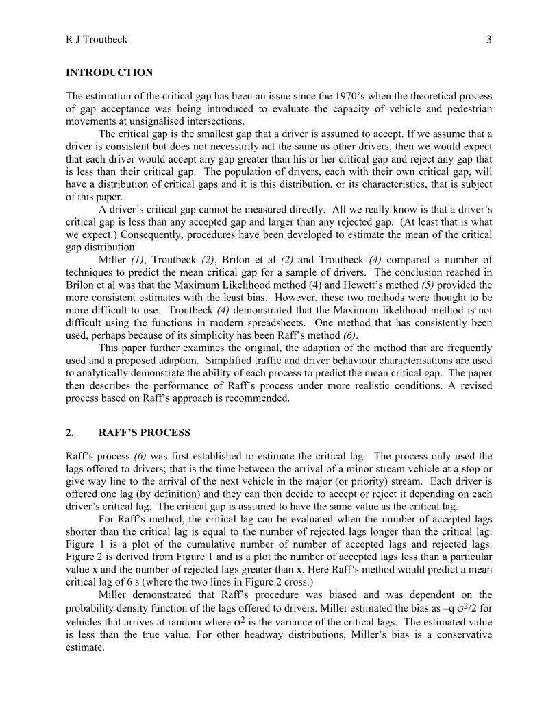
Raff’s process (6) was first established to estimate the critical lag. The process only used the lags offered to drivers; that is the time between the arrival of a minor stream vehicle at a stop or give way line to the arrival of the next vehicle in the major (or priority) stream. Each driver is offered one lag (by definition) and they can then decide to accept or reject it depending on each driver’s critical lag. The critical gap is assumed to have the same value as the critical lag. For Raff’s method, the critical lag can be evaluated when the number of accepted lags shorter than the critical lag is equal to the number of rejected lags longer than the critical lag. Figure 1 is a plot of the cumulative number of number of accepted lags and rejected lags. Figure 2 is derived from Figure 1 and is a plot the number of accepted lags less than a particular value x and the number of rejected lags greater than x. Here Raff’s method would predict a mean critical lag of 6 s (where the two lines in Figure 2 cross.) Miller demonstrated that Raff’s procedure was biased and was dependent on the probability density function of the lags offered to drivers. Miller estimated the bias as –q σ2/2 for vehicles that arrives at random where σ2 is the variance of the critical lags. The estimated value is less than the true value. For other headway distributions, Miller’s bias is a conservative estimate.

R J Troutbeck 4

FIGURE 1 Cumulative number of accepted and rejected lags

FIGURE 2 Number of accepted lags greater than a particular lag time, x, and the number of rejected lags less than x.

In the following sections, Raff type processes are discussed analytically using an assumed uniform distribution of drivers’ critical gaps and an exponential distribution for the headways in the major stream.

0 10 20 30 40 50 60 70 80

0 2 4 6 8 10 12 14 16 18

Cum

ulat

ive

num

ber o

f lag

s

Lag times (s)

Accepted lags Rejected lags

0

10

20

30

40

50

60

70

80

0 2 4 6 8 10 12 14 16 18

Num

ber o

f lag

s

Lag times (s)

Accepted lags greater than x Rejected lags less than x

R J Troutbeck 5

RAFF’S ORIGINAL PROCESS

Raff process involves the analysis of lags, which has a probability density function given by:

l(t) = q[1 – F(t)] (1) where F(t) is the cumulative probability distribution of headways in the major stream with a flow of q. Each driver observes one lag and either accepts it or rejects it. The cumulative number of accepted lags less than or equal to t is given by:

NA(x) = N g(T ) l(t) dT dt0

t∫

0

x∫ (2)

where N is the total number of drivers. Similarly, the cumulative number of rejected lags less than or equal to t is given by:

NR(x) = N g(T ) l(t) dT dtt

∞∫

0

x∫ (3)

For this analysis, the headways in the major stream are assumed to have a negative exponential distribution and the critical gaps are uniformly distributed between c1 and c2. The distribution of lags is also has a negatively exponential distribution with

l(t) = f (t) = qe−qt (4)

The probability density function for the critical gaps is:

g(g) = 1c2 − c1

for c1 < g < c2 (5)

The cumulative number of accepted lags and rejected lags is given below. NA(x) = 0 for x ≤ c1

NA(x) = N (qc1 − qx −1)e−qx + e−qc1

q(c2 − c1) for c1 < x < c2 (6)

NA(x) = N (qc1 − qc2 )e−qx + e−qc1 − e−qc2

q(c2 − c1) for x ≥ c2

and

NR(x) = N(1− e−qx ) for x ≤ c1

NR(x) = N (qx −1− qc2)e−qx − e−qc1 + q(c2 − c1)q(c2 − c1)

for c1 < x < c2 (7)

NR(x) = N e−qc2 + e−qc1 + q(c2 − c1)q(c2 − c1)

for x ≥ c2

R J Troutbeck 6

Using Raff’s original formulation (6), the critical lag is when the number of accepted lags shorter than x is the same as the number of rejected lags longer than x. That is when NA(x0) is equal to NR(∞)-NR(x0). Substituting in the expressions for NA(x) and NR(x) gives the relationship for x0:

e−qc1 − e−qc2 = q(c2 − c1)e−qx0

or with some manipulation:

x0 = c1 −1qln 1− e

−q(c2−c1)

q(c2 − c1)

"

#$$

%

&'' (8)

Using a series expansion for the exponential and the logarithm functions gives the approximation:

x0 ≈(c1+ c2 )2

−q(c2 − c1)

2

24+q3(c2 − c1)

4

2880… (9)

Given that the mean and variance of the uniformly distributed critical gaps are:

mg =(c1+ c2 )2

σg2 =

q(c2 − c1)2

12

then

x0 ≈ mg −q σg

2

2+q3 σg

4

20…

(10)

Miller (1) evaluated Raff’s procedure and also developed equation 10 and indicated that it could be applied when other headway and critical gap distributions were assumed. For the case where the critical gaps were uniformly distributed between 4 and 8 s and the major stream headways had an exponential distribution, a linear approximation (from the first two terms of equations 9 or 10) had an error of less than 0.01 s. The bias with Raff’s method could be corrected but it requires an estimate of the variance of the critical gaps. Unfortunately Raff’s method does not provide a procedure to estimate this variance.

RAFF’S PROCESS AS CURRENTLY USED

Researchers frequently use the Raff method (7, 8, 9) by comparing the distributions for all accepted and the rejected gaps to estimate the mean critical gap

R J Troutbeck 7

Accepted Gap and Rejected Gap Distributions

Assume that F(t) is the cumulative distribution of the gaps in the major stream and that T is the critical gap of a driver. Further, A(t|T) is the cumulative probability function for accepted gaps given a critical gap of T.

A(t |T ) = f (t)1−F(T )T

t∫ dt for t ≥ T

A(t |T ) = F(t)−F(T )1−F(T )

for t ≥ T

A(t|T) = 0 otherwise (11) Using the probability density function of the critical gaps, g(T) and a(x|T) as the probability density function for accepted gaps given a critical gap, T, then the distribution of all accepted gaps is A(t) is:

A(x) = g(T ) a(t |T ) dT dt0

t∫

0

x∫ (12)

Similarly, R(t|T) and r(t|T) are the cumulative probability function and the probability density function of rejected gaps given a critical gap of T.

R(t |T ) = F(t)F(T )

for t < T

R(t|T) = 1 otherwise (13) Depending on the critical gap, some drivers might reject more than one gap. Therefore we need to include the average number of rejected gaps. Probability of not rejecting a gap is [1-F(T)] Probability of rejecting 1 gap is [1-F(T)] F(T) Probability of rejecting 2 gaps is [1-F(T)] F(T)2 …. Probability of rejecting n gaps is [1-F(T)] F(T)n Summing over all possibilities gives the average number of gaps rejected for a critical gap of T.

n(T ) = F(t)1−F(T )

(14)

Number of rejected gaps for a critical gap of T and of size t, nr(t|T), is given by

nr(r |T ) = r(t |T ) n(T ) = f (t)1−F(T )

(15)

The average number of rejected gaps per driver is N and is given by

R J Troutbeck 8

N = g(t) n(t)dt0

∞∫ (16)

The distribution of the rejected gaps is

R(x) = 1N

g(T ) nr(t |T ) dT dtt

∞∫

0

x∫ (17)

Critical Gap Assuming Uniformly Distributed Critical Gaps and Exponential Headways

If the major stream headways have a negative exponential distribution and the critical gaps have a uniform distribution between c1 and c2

then the cumulative distributions of accepted gaps and

rejected gaps are:

A(x) = 0 for x ≤ c1

A(x) = q(x − c1)−1+ e−q(x−c1)

q(c2 − c1) for c1 < x < c2 (18)

A(x) = q(c2 − c1)+ e−q(x−c1) − e−q(x−c2 )

q(c2 − c1) for x ≥ c2

and

R(x) = eqc2 − eqc1 − e−qx (eqc2 − eqc1 )eqc2 − eqc1 − q(c2 − c1)

for x ≤ c1

R(x) = eqc2 − eqc1 − e−qxeqc2 +1+ qc1 − qx

eqc2 − eqc1 − q(c2 − c1) for c1 < x < c2 (19)

R(x) = 1 for x ≥ c2

Note that the average number of rejected gaps per driver is:

N =eqc2 − e−qc1 − q(c2 − c1)

q(c2 − c1) (20)

A typical method of using Raff’s process is to estimate the critical gap when the proportion of accepted gaps shorter than x0 is the same as the proportion of rejected gaps longer than x0. That is when A(x0) = 1 – R(x0). That is when:

q(x0 − c1)−1+ e−q(x0−c1)

q(c2 − c1)=1− e

qc2 − eqc1 − e−qxeqc2 +1+ qc1 − qx0eqc2 − eqc1 − q(c2 − c1)

(21)

This equation can be expressed as

R J Troutbeck 9

q(x0 − c2 )−1+ e−q(x0−c2 )

q(x0 − c1)−1+ e−q(x0−c1)

=eqc2 − eqc1 − q(c2 − c1)

q(c2 − c1) (22)

Expanding the exponentials on the right side gives

RHS = q2(c2 + c1)2!

+q3(c1

2 + c1c2 + c22)

3!+q4(c1

3 + c12c2 + c1c2

2 + c23)

4!+… (23)

When q approaches zero, the RHS approaches 0 and the LHS is equal 0 when the estimate of the critical gap x0 is c2. For q large, the RHS is also large (approaching ∞) and the LHS is also large when x0 is equal to c1. Consequently the estimated mean critical gap from this method can result in values ranging from the minimum to the maximum critical gaps values as shown in Figure 3.

Raff’s method with the number of accepted and rejected gaps

Patil and Pawer (10) used another variation of Raff’s method. They defined the critical gap as the gap size that has the same number of accepter gaps less than it as the number of rejected gaps greater than it. This is the same as the original method but using all gaps rather than lags. Typically it has been found that better estimates of the critical gap are provided by techniques that give the same weight to each driver. A driver rejects a larger number of gaps at higher major stream flows. An increase in the number of rejected gaps generally increases the bias as major stream flows increases. The number of accepted gaps is given by n A(X) where n in the number of drivers observed and A(x) is the distribution of accepted gaps given the three-part equation 18. The number of rejected gaps is also given by the equations presented above and is n N R(x) with N given by equation 20 and R(x) given by equation 19. The process used by Patil and Pawer derived the critical gaps using the equation:

n A(x0) = n N − n N R(x0) (24)

Or more specifically, for exponential traffic and uniformly distributed critical gaps, the estimated critical gap, t0 from this approach is

x0 = −1qln q(c2 − c1)

eqc2 − eqc1"

#$

%

&' (25)

Estimates from this equation are shown in Figure 3 below. The lines in Figure 4 are transforms of those in Figure 3 using the variable:

z = x0 − c1c2 − c1

(26)

The lines in Figure 4 while not coincident do show similar trends.

RAFF’S PROCESS USING THE MAXIMUM REJECTED GAP

The distribution of rejected gaps given a critical gap of T is given by equations 13 and 15. This distribution will be used to evaluate the maximum rejected gap distribution.

R J Troutbeck 10

If X and Y are two distributions with CDF’s of X(x) and Y(y) and variable z is the maximum of x and y, then the probability that z is less than a particular value requires both x and y to be less than that same value. That is the CDF of z, Z(z) is equal to the product of X(z) and Y(z).

FIGURE 3 The estimated mean critical gap from Raff’s original method, Raff’s method based on the distributions of accepted and rejected gaps, and Raff’s method based on the

number of accepted gaps and the number of rejected gaps.

0 300 600 900 1200 1500 1800Major stream flow (veh/h)

Estim

ated

mea

n cr

itica

l gap

(s)

8.0

7.0

6.0

5.0

7.0

6.0

5.0

4.0

8.0

7.0

6.0

5.0

4.0

3 to 8 s

3 to 7 s

4 to 8 s

Original Raff procedure

Using accepted and rejected gap distributions

Using accepted and rejected gap numbers

R J Troutbeck 11

FIGURE 4 The relationship of the critical gap dimension z and the major stream flow for Raff’s original method, Raff’s method based on the distributions of accepted and rejected

gaps, and Raff’s method based on the number of accepted gaps and the number of rejected gaps. The critical gap distributions are those described in Figure 3.

The probability of a gap being accepted is 1-F(T) and the probability of a gap being rejected is F(T). The probability that the first gap is accepted is 1-F(T) and the maximum rejected gap is listed as zero. The probability that n gaps are rejected before the next gap is accepted is [1-F(T)] F(T)n. The CDF of the maximum of n rejected gaps is given by R(t|T)n. Summing over all possible values of n gives Rm(x|T) being the cumulative distribution of the maximum rejected gaps given a critical gap of T. That is:

Rm(x |T ) = [1−F(T )]+[1−F(T )]F(T ) R(x |T )…+[1−F(T )]F(T )n R(x |T )n… (27)

This is a geometric series giving

Rm(x |T ) =1−F(T )1−F(x)

For 0 ≤ x ≤T (28)

The reader will note that there are 1-F(T) values of 0 for the drivers that do not reject a gap and there is one rejected gap value per driver. Assuming that the major stream headways have an exponential distribution and that the critical gaps are uniformly distributed between c1 and c2 then the distribution for the maximum rejected gap is given by:

0.2

0.4

0.6

0.8

1

0 300 600 900 1200 1500 1800

Crit

ical

gap

dim

ensi

on, z

Major strem flow (veh/h)

Original Gap distributions Gap Numbers

R J Troutbeck 12

Rm(x) =eqx (e−qc1 − e−qc2 )

q(c2 − c1) for x ≤ c1

Rm(x) =1+ q(x − c1)− e

−q(c2−x)

q(c2 − c1) for c1 < x < c2 (29)

Rm(x) = 1 for x ≥ c2

The distribution of the maximum rejected gap defined in equation 29 and the accepted gap distribution defined in equation 18, can be used to estimate the mean critical gap by equating the proportion of accepted gaps shorter than x0 to the proportion of rejected gaps longer than x0. That is when A(x0) is equal to 1 – Rm(x0) or when

q(x0 − c1)+ e−q(x0−c1) = q(c2 − x0)+ e

−q(c2−x0 ) (30)

This occurs when x0 is (c1+c2)/2 which is the mean of the critical gap distribution. The reader will note that the equation is independent of the major stream flow q and that the results are unbiased. Raff’s approach using the maximum rejected gap provides the unbiased estimates for random arrivals on the major stream and for the critical gaps to be uniformly distributed.

PROPOSED RAFF’S PROCESS FOR MORE GENERAL CONDITIONS

A simulation process has been used in the past to evaluate different techniques for estimating the critical gap. Miller (1), Troutbeck (2) and Brilon et al (3) and Troutbeck (4) have used this technique to evaluate a number of previous techniques. For this process: 1. Critical gaps were assigned to a number drivers based on a specified distribution. 2. Gaps in traffic are simulated using an established headway distribution. 3. The duration of the accepted and rejected gaps are recorded. 4. The mean critical gap was calculated based on Raff’s procedure. This process was applied to a range of traffic flows and the critical gap distributions. The lines in Figure 5 are generated using equations 8, 22 and 28. The data points are from the simulation of exponential traffic and uniformly distributed critical gaps between 4 and 8 s. The mean critical gap was 6 s in all cases. The simulation results are close to the values from the equations (as they should be). The effects of the random process were minimized with a sample size of 100,000 drivers.

EFFECT OF THE CRITICAL GAP DISTRIBUTION AND HEADWAY DISTRIBUTION ON RAFF’S ESTIMATES

Other critical gap distributions considered are:

R J Troutbeck 13

• Triangular distribution with a minimum of 4 s, a maximum of 8 s, and a mode of 6 s giving a mean of 6 s and a standard deviation of √12/√18 or 0.816 s. • Triangular distribution with a minimum of 4 s, a maximum of 9 s and a mode of 5 s giving a mean of 6 s and a standard deviation of √21/√18 or 1.080 s • Triangular distribution with a minimum of 3 s, a maximum of 8 s and a mode of 7 s giving a mean of 6 s and a standard deviation of √21/√18 or 1.080 s • Normal distribution with a mean of 6 s and a standard deviation of 1.2 s • Log-Normal distribution with a mean of 6 s and a standard deviation of 1.2 s • Weibull distribution with a mean of 6 s and a standard deviation of 1.16 s

FIGURE 5 Values from equations (lines) and simulation results (data points) for Raff’s

technique. The estimated critical gap for 100,000 drivers was calculated using Raff’s method and the maximum rejected gap and the accepted gap for each driver. (A large sample size was used to minimize the effects of the random process.) Figure 6 shows the predicted critical gap when the critical gap distribution was either a symmetric triangular distribution or an asymmetric triangular distribution. The symmetrical distributions gave values very close to the 6 s; the predetermined mean critical gap for all distributions. It is apparent that the triangular distribution that has the mode closer to the maximum value (that is with negative skewness) produces estimates that increase above the predetermined mean as the flow increases. Similarly the triangular distribution that has positive skewness has the opposite effect. Figure 7 shows the results for a Normal, log-Normal or Weibull distribution and the shows the same effect of skewness. The Wiebull has negative skewness, while the log Normal has positive skewness. The bias caused by the skewness of the distribution is small (less than 0.05 s). The bias is proportional to the major stream flow and approximately a cubic relationship with the distribution skewness. It has been generally considered that the critical gap distribution will have a positive skew. There is a limit to the duration of the smaller acceptable gaps and some drivers will have

4.5

5

5.5

6

6.5

7

0 300 600 900 1200 1500 1800

Estim

ated

crit

ical

gap

(s)

Major stream flow (veh/h)

Traditional All rejected gaps Maximum rejected gap

R J Troutbeck 14

much larger critical gaps than the modal value. The Normal and the Weibull distributions do not support this requirement.

FIGURE 6 Estimates of the critical gap for different triangular critical gap distributions.

FIGRE 7 Estimates of the critical gap for different headway distributions.

Figure 8 shows the estimates of the critical gap when the major stream has a Cowan M3 distribution (11), which allows for vehicles to arrive in bunches and provides a better representation of headways in higher flows. In this figure, the critical gap distribution was either uniform or log-Normal. Comparing Figures 7 and 8 show that the bias is similar for the major stream headways with a Cowan M3 distribution or an exponential distribution. In either case, the bias is less than 0.05 (based on the results of the simulations presented here). The estimated critical gap is unaffected by the major stream headway distribution.

5.9

5.95

6

6.05

6.1

0 200 400 600 800 1000 1200 1400 1600 1800

Estim

ated

crit

ical

gap

(s)

Major stream flow (veh/h)

Traingular 4 5 9 Triangular 4,6,8 Triangular 3,7,8

5.9

5.95

6

6.05

6.1

0 200 400 600 800 1000 1200 1400 1600 1800

Estim

ated

crit

ical

gap

(s)

Major stream flow (veh/h)

Uniform Log-Normal Weibull Normal

R J Troutbeck 15

FIGURE 8 Estimated critical gap using Raff’s method and the maximum rejected gap and Cowan headway distribution for the gaps in the major stream. The expected mean critical

gap is 6.0 s.

COMPARISON BETWEEN RAFF’S ESTIMATE AND THE MAXIMUM LIKELIHOOD METHOD

Troutbeck (4) examined the performance of the Maximum Likelihood method for estimating the size of the critical gap. The ML method has previously been found to be one of the better methods for estimating the critical gap. It was the method used to evaluate critical gaps for unsignalised intersections in the HCM (12). Here the critical gap of 100 drivers was chosen, traffic was simulated and the observed accepted and maximum rejected gaps were used to calculate the estimate of the mean critical gap. This is repeated 100 times to provide the mean of 100 estimates, which could then be compared with the mean of the values originally used for the simulated drivers. The variance of the estimates of the mean can be used to establish the consistency of the estimates. Figure 9 demonstrates the estimates of the mean critical gap from the maximum likelihood method are better than those from Raff’s method using the maximum rejected gap. However, Raff’s method still provides useful and generally acceptable estimates even though there is an increasing bias as the flow increases. The maximum likelihood method also provides an estimate of the standard deviation of the critical gap to better describe the distribution. Troutbeck (4) also provided an examination of the performance of the Maximum Likelihood method when drivers were inconsistent. In this analysis, drivers rejected 10 per cent of the gaps between their critical gap and twice their critical gap. (Traditionally these gaps would have been accepted.) All gaps greater than twice a driver’s critical gap were accepted. When applying the same approach, Raff’s method using the maximum rejected critical gap estimates are closer to the actual critical gap values than the Maximum Likelihood method. See Figure 10.

5.9

5.95

6

6.05

6.1

0 200 400 600 800 1000 1200 1400 1600 1800

Estim

ated

crit

ical

gap

(s)

Major stream flow (veh/h)

Uniform log-Normal

R J Troutbeck 16

FIGURE 9 Estimated critical gap using Raff’s method with the maximum rejected gap

and the Maximum likelihood method.

FIGURE 10 Estimated critical gap using Raff’s method and the maximum rejected gap and Cowan headway distribution for the gaps in the major stream and where drivers are

inconsistent.

CONCLUSIONS

Given exponential headways in the major stream, and a uniform distribution of headways, it was found that unbiased estimates of the critical gap would be obtained using a modified version of Raff’s method involving the accepted gap and the maximum rejected gap. (Note that for an individual driver, the maximum rejected gap could be greater than the accepted gap.) The bias in the original formulation has been found to agree with an analysis by Miller (1). A commonly used procedure, based on Raff’s method, equates the critical gap, x0, to the

5.5 5.6 5.7 5.8 5.9

6 6.1 6.2 6.3 6.4 6.5

0 200 400 600 800 1000 1200 1400 1600 1800

Mea

n of

100

est

imat

es o

f the

m

ean

criti

cal g

ap (s

)

Major stream flow (veh/h)

MLH Raff True mean

5.8 5.9

6 6.1 6.2 6.3 6.4 6.5 6.6 6.7 6.8

0 200 400 600 800 1000 1200 1400 1600 1800

Mea

n of

100

est

imat

es o

f the

m

ean

criti

call

gap

(s)

Major stream flow (veh/h)

MLH Raff True mean

R J Troutbeck 17

point when the proportion of accepted gaps greater than x0 and the proportion of rejected gaps less than x0 are equal. This common procedure has been demonstrated to have a large bias that is dependent on the major stream flow. An analysis of the distributions for the accepted gaps and the maximum rejected gaps demonstrated that the Raff’s technique produced the correct result if the critical gaps were uniformly distributed and the major stream headways were exponentially distributed. Simulation results demonstrated that if the critical gap distribution had positive skew, the bias in the estimates of the critical gap increased with the major stream flow. Raff’s method tended to slightly underestimate the true mean critical gap. The estimates of the critical gap from Raff’s method using the maximum rejected gap are slightly inferior to those using the Maximum Likelihood method (4). The difference is not great and this application of Raff’s method may be more suitable to some studies, particularly as it will provide an answer so long as some accepted gaps are less than some maximum rejected gaps. It would only be in extreme conditions where this would not occur. Accordingly, if gap acceptance values are required for HCM analyses, then Raff’s method using the maximum rejected gap provides acceptable values. It is recommended that the Maximum Likelihood method be the preferred technique but that results using the maximum rejected gaps with Raff’s technique be accepted.

REFERENCES

1. Miller, A. J. Nine Estimators of Gap Acceptance Parameters. In 'Traffic Flow and Transportation' (Ed. Newell). Proc Int. Symp. on the Theory of Traffic Flow and Transpn. Berkeley, June 1971. American Elsevier Publishing Co. 1972

2. Troutbeck, R. J. A Review of the Ramsey-Routledge Method for Gap Acceptance Times. Traffic Engineering & Control, 16(9), pp. 373-5. 1975

3. Brilon,W., N. Keonig, and R J Troutbeck. Useful Estimating Procedures for Critical Gaps. Transportation Research A33(3/4) 1999 pp 217-236

4. Troutbeck, R. J. Estimating the Mean Critical Gap. In Transportation Research Record: Journal of the Transportation Research Board, No. 2461, Transportation Research Board of the National Academies, Washington, D.C., 2014, pp 76-84,

5. Hewitt, R. H. Measuring Critical Gap. In Transportation Science 17(1). 1983 pp. 87-109 6. Raff, M. S. A Volume Warrant for Urban Stop Signs Eno foundation, Saugatuck, USA.

1950. 7. Bai, Y., X. He, L. Long, and X. Yang. Study on Pedestrian Red Light Crossing Violation.

Presented at 92nd Annual Meeting of the Transportation Research Board, Washington, D.C., 2013 Paper # #13-3645 (2013

8. Dahl, J., and C. Lee. Empirical Estimation of Capacity for Roundabouts Using Adjusted Gap-Acceptance Parameters for Trucks. Presented at 91st Annual Meeting of the Transportation Research Board, Washington, D.C., 2012 Paper #12-3519

9. Lee, C., and M. N. Khan Prediction of Capacity for Roundabouts based on Percentages of Trucks in Entry and Circulating Flows, Presented at 92nd Annual Meeting of the Transportation Research Board, Washington, D.C., 2013, Paper #13-1391

R J Troutbeck 18

10. Patil, G., D. S. Pawar. Temporal and Spacial Gap Acceptance for Minor Road at Uncontrolled Intersections in India. In Transportation Research Record: Journal of the Transportation Research Board, No. 2461, Transportation Research Board of the National Academies, Washington, D.C., 2014, pp 129-136,

11. Cowan, R. J. (1975) Useful Headway Models. In Transpn Res., 9(6), 12. Kyte, M., Z. Tian, Z. Mir, Z. Hameedmansoor, W. Kittelson, M. Vandehey, B. Robinson,

W. Brilon, L. Bondzio, N. Wu, and R. Troutbeck. (1975) NCHRP Web Document 5: Capacity and Level of Service at Unsignalized Intersections: Final Report, Vol. 1. Two-way Stop-Controlled Intersections. Transportation Research Board, Washington, D.C