reversible space–time simulation of cellular automata

Theoretical Computer Science 246 (2000) 117–129www.elsevier.com/locate/tcs

Reversible space–time simulation of cellular automata

J�erome O. Durand-Lose 1

Laboratoire 13S, CNRS UPREES-A 6070, 930 Route des Colles, BP 145,06903 SOPHIA ANTIPOLIS Cedex, France

Received July 1997; revised October 1998Communicated by M. Nivat

Abstract

The goal of this paper is to design a reversible d-dimensional cellular automaton which iscapable of simulating the behavior of any given d-dimensional cellular automaton over any givencon�guration (even in�nite) with respect to a well suited notion of simulation we introduce. Wegeneralize a problem which was originally addressed in a paper by To�oli in 1977. He askedwhether a d-dimensional reversible cellular automaton could simulate d-dimensional cellularautomata. In the same paper he proved that there exists a (d+1)-dimensional reversible cellularautomaton which can simulate a given d-dimensional cellular automaton. To prove our result,we use as an intermediate model partition cellular automata de�ned by Morita et al. in 1989.c© 2000 Published by Elsevier Science B.V. All rights reserved.

Keywords: (Partitioned) Cellular automata; Space–time simulation; Intrinsic universalityand reversibility

1. Introduction

“Is it possible to capture the behavior of a discrete system with another one whichis reversible?” We answer a�rmatively in the case of cellular automata.Reversible systems are of interest since they preserve information and energy and

allow unambiguous backtracking. They are studied in computer science in order todesign computers which would consume less energy.Cellular automata (CA), a model of computation introduced by Ulam and

von Neumann in the 1950s, model massively parallel computations and physical phe-nomena. A CA can be considered as a bi-in�nite array of dimension d whose elementsare called cells. Each cell takes a value from a �nite set of states S. A con�guration

E-mail address: [email protected] (J.O. Durand-Lose).1 This work was done while the author was in LaBRI, Universit�e Bordeaux I, France.

0304-3975/00/$ - see front matter c© 2000 Published by Elsevier Science B.V. All rights reserved.PII: S0304 -3975(99)00075 -4

118 J.O. Durand-Lose / Theoretical Computer Science 246 (2000) 117–129

is a valuation of the whole array. A CA updates its con�guration by synchronouslychanging the state of each cell according to its neighbor cells with respect to a lo-cal transition function. All the cells use the same local transition function. Thus theupdate process is parallel, synchronous, local and uniform. From the local transitionfunction f, one can de�ne a corresponding global transition function F over thecon�gurations.A CA is reversible when its global transition function F is bijective and F−1 is

the global transition function of some CA. The study of CA reversibility started inthe 1960s. It is known that if F is one-to-one then it is bijective [10, 13] and thecorresponding CA is reversible [5, 14]. If the reversibility of CA is proved decidablein dimension 1 [1], this is not anymore true for greater dimensions [7].In 1977, To�oli [15] proved that any CA can be simulated by a reversible CA

(R-CA) one dimension higher and that there are two-dimensional R-CA which arecomputation universal. It was only in 1992 that the existence of a computation universalR-CA was proved in dimension 1 by Morita [11]. To do this he introduced partitionedcellular automata (PCA). In PCA the state of each cell is partitioned according to theneighborhood. Each cell exchanges parts of its state with the neighbor cells and thencomputes its new state.In [2], we proved that there are R-CA able to simulate in linear time any R-CA of

the same dimension (greater than 2), over any con�guration (even in�nite). This resulthas been extended to dimension 1 in 1997 [3] with the use of PCA.Yet, it is unknown whether it is possible to simulate any CA with a R-CA of the same

dimension. In 1995, Morita [12] proved that it is possible over �nite con�gurations,i.e. con�gurations such that there are �nitely many cells which are not in a givenstate q. Finite con�gurations form a strict subset of recursive con�gurations which isitself far from being the whole set of con�gurations. Finiteness is also too restrictivefor physicians and mathematicians.Intuitively, a simulation of a machine B by a machine A is some construction which

shows that everything machine B can do on input x can be performed as well bymachine A on the same input. We generalize this intuitive notion to space–time sim-ulation. For a CA A, a space–time diagram depicts the whole computation of A onan input c0. It corresponds to the sequence of all the con�gurations of A starting withc0. Space–time diagrams serves as a tool for designing CA (e.g. see [4, 8, 9, 6]). Ournotion of space–time simulation of B by A de�nes an embedding relation between thespace–time diagram of B and the space–time diagram of A.Our main result states that any d-dimensional CA (d-CA) can be space–time sim-

ulated by a d-R-PCA. We give a proof for the one-dimensional case and sketch thegeneralization to higher dimensions. As a corollary, we prove that any d-CA can besimulated by a d-R-CA since any d-R-PCA is indeed a particular d-R-CA. Then, asa conclusion, we state that there exists a d-R-CA which is capable of space–timesimulating any d-CA.

J.O. Durand-Lose / Theoretical Computer Science 246 (2000) 117–129 119

2. De�nitions

Con�gurations are bi-in�nite arrays of �nite dimension d. Points of con�gurationsare called cells. Each cell takes a value from a �nite set of states S. The set of allcon�gurations is denoted by C (C= SZ

d). The state of cell x in con�guration c is

denoted cx. Cellular automata (CA) and partitioned cellular automata (PCA) update allthe cells of a con�guration in a parallel, synchronous local and uniform way.

2.1. Cellular automata

A d-dimensional cellular automaton (d-CA) is de�ned by (S;N; f). The neighbor-hood N is a �nite subset of Zd. The local transition function f : SN → S yields thenew state of a cell according to the states of the cells in its neighborhood. The globaltransition function F :C→C updates con�gurations as follows:

∀c∈C; ∀x∈Zd; (F(c))x =f((cx+�)�∈N):

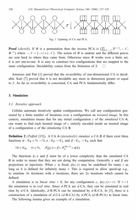
The new state of a cell only depends on the neighbor cells as described in Fig. 1 (left).

2.2. Partitioned cellular automata

According to Morita’s de�nition [11, 12], a d-dimensional partitioned cellularautomaton (d-PCA) is a special form of CA de�ned by (S;N; �). The set of states isa cartesian product of sets indexed by the neighborhood: S =

∏�∈N S(�). The � com-

ponent of a state s is denoted by s(�). The state transition function � operates overS. The global transition function F is de�ned by

∀c∈C; ∀x∈Zd; F(c)x =�( ∏

�∈N

c(�)x+�

):

Equivalently, each state is the product of the information to be exchanged. Each com-ponent is sent to a single cell. An intermediate state is formed by grouping what isleft and what is received. The state transition function � yields the new state fromthe intermediate state. The cell only keeps a partial knowledge about its own state andonly receives a partial knowledge about the states of the neighbor cells, as depicted inthe right part of Fig. 1.

2.3. Reversibility

A CA (PCA) is reversible if its global transition function F is a bijection and itsinverse F−1 is the global transition function of some CA (PCA). We denote R-CA(R-PCA) reversible CA (PCA). For PCA, the following lemma holds in any dimension.

Lemma 1. A PCA is reversible if and only if its state transition function � is apermutation; which is decidable.


Fig. 1. Updating of CA and PCA.

Proof (sketch). If � is a permutation then the inverse PCA is (∏

�∈−N S(−�);−N;�−1) where −N= {−� | �∈N}. The action of � is undone and the di�erent piecesare sent back to where they came from. Otherwise since � works over a �nite set,it is not one-to-one. It is easy to construct two con�gurations that are mapped to thesame con�guration. Decidability comes from the �niteness of S.

Amoroso and Patt [1] proved that the reversibility of one-dimensional CA is decid-able. Kari [7] proved that it is not decidable any more in dimension greater or equalto 2. As far as reversibility is concerned, CA and PCA fundamentally di�er.

3. Simulation

3.1. Iterative approach

Cellular automata iteratively update con�gurations. We call any con�guration gen-erated by a �nite number of iterations over a con�guration an iterated image. In thiscontext, simulation means that for any initial con�guration c of the simulated CA A,one wants to �nd each iterated image of c entirely encoded inside an iterated imageof a con�guration e of the simulating CA B.

De�nition 2 (To�oli [15]). A CA A (iteratively) simulate a CA B if there exist threefunctions : CB×N→N; � : CB→CA and � : CA→CB such that

∀b∈CB; ∀t ∈N; FtB(c)= � ◦F (c; t)

A ◦ �(b):

The functions ; � and � must be of a lower complexity than the simulated CAB in order to insure that they are not doing the computation. Generally � and � areprojections or injections. When c is �xed, (c; t) may be unde�ned for many t aslong as it is de�ned for in�nitely many t. This is required to allow speed-up e.g.,to simulate 3n iterations with n iterations, there are 2n iterations which cannot bede�ned.A simulation is in linear time � if, for any con�guration c, (c; t)= � t. If �=1

the simulation is in real time. Since d-PCA are d-CA, they can be simulated in realtime by d-CA. Identically, d-R-PCA can be simulated by d-R-CA. In [3], there is aconstruction of a simulation of d-CA (d-R-CA) by d-PCA (d-R-PCA) in linear time.The following lemma gives an example of a simulation.


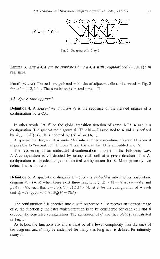
Fig. 2. Grouping cells 2 by 2.

Lemma 3. Any d-CA can be simulated by a d-CA with neighborhood {−1; 0; 1}d inreal time.

Proof (sketch). The cells are gathered in blocks of adjacent cells as illustrated in Fig. 2for N= {−2; 0; 1}. The simulation is in real time.

3.2. Space–time approach

De�nition 4. A space–time diagram A is the sequence of the iterated images of acon�guration by a CA.

In other words, let F be the global transition function of some d-CA A and a acon�guration. The space–time diagram A :Zd ×N→ S associated to A and a is de�nedby Ax; t =(Ft(a))x. It is denoted by (F; a) or (A, a).A space–time diagram B is embedded into another space–time diagram B when it

is possible to “reconstruct” B from A and the way that B is embedded into A.The recovering of an embedded B-con�guration is done in the following way.

A A-con�guration is constructed by taking each cell at a given iteration. This A-con�guration is decoded to get an iterated con�guration for B. More precisely, wede�ne this as follows:

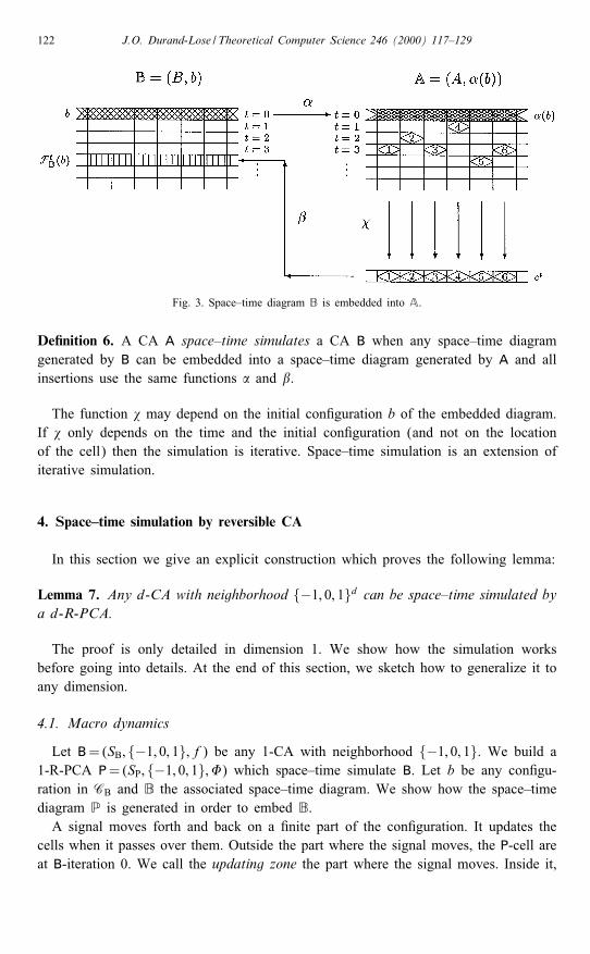
De�nition 5. A space–time diagram B=(B; b) is embedded into another space–timediagram A=(A; a) when there exist three functions � :Zd ×N→N; � :CB→CA and� :CA→CB such that a= �(b); ∀(x; t)∈Zd ×N, let ct be the con�guration of A suchthat ctx =Ax; �(x; t); ∀t ∈N, Ft

B(b)= �(ct).

The con�guration b is encoded into a with respect to �. To recover an iterated imageof b, the function � indicates which iteration is to be considered for each cell and �decodes the generated con�guration. The generation of ct and then Ft

B(b) is illustratedin Fig. 3.As before, the functions �; � and � must be of a lower complexity than the ones of

the diagrams and ct may be unde�ned for many t as long as it is de�ned for in�nitelymany t.


Fig. 3. Space–time diagram B is embedded into A.

De�nition 6. A CA A space–time simulates a CA B when any space–time diagramgenerated by B can be embedded into a space–time diagram generated by A and allinsertions use the same functions � and �.

The function � may depend on the initial con�guration b of the embedded diagram.If � only depends on the time and the initial con�guration (and not on the locationof the cell) then the simulation is iterative. Space–time simulation is an extension ofiterative simulation.

4. Space–time simulation by reversible CA

In this section we give an explicit construction which proves the following lemma:

Lemma 7. Any d-CA with neighborhood {−1; 0; 1}d can be space–time simulated bya d-R-PCA.

The proof is only detailed in dimension 1. We show how the simulation worksbefore going into details. At the end of this section, we sketch how to generalize it toany dimension.

4.1. Macro dynamics

Let B=(SB; {−1; 0; 1}; f) be any 1-CA with neighborhood {−1; 0; 1}. We build a1-R-PCA P=(SP; {−1; 0; 1}; �) which space–time simulate B. Let b be any con�gu-ration in CB and B the associated space–time diagram. We show how the space–timediagram P is generated in order to embed B.A signal moves forth and back on a �nite part of the con�guration. It updates the

cells when it passes over them. Outside the part where the signal moves, the P-cell areat B-iteration 0. We call the updating zone the part where the signal moves. Inside it,


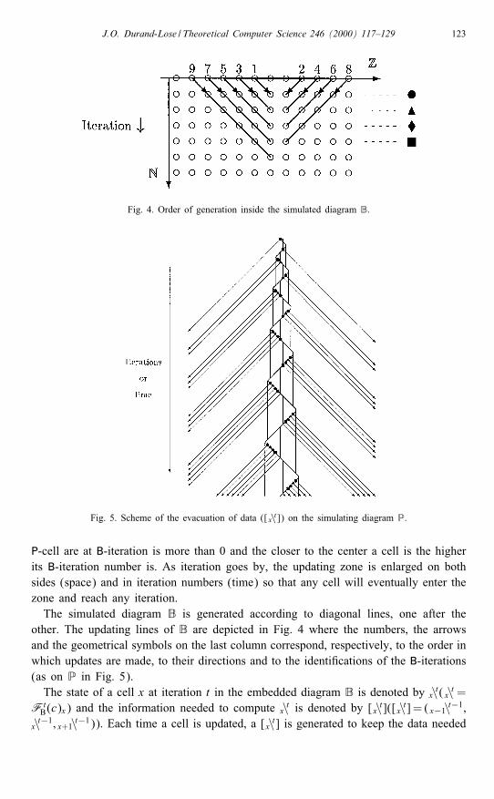
Fig. 4. Order of generation inside the simulated diagram B.

Fig. 5. Scheme of the evacuation of data ([ x\t ]) on the simulating diagram P.

P-cell are at B-iteration is more than 0 and the closer to the center a cell is the higherits B-iteration number is. As iteration goes by, the updating zone is enlarged on bothsides (space) and in iteration numbers (time) so that any cell will eventually enter thezone and reach any iteration.The simulated diagram B is generated according to diagonal lines, one after the

other. The updating lines of B are depicted in Fig. 4 where the numbers, the arrowsand the geometrical symbols on the last column correspond, respectively, to the order inwhich updates are made, to their directions and to the identi�cations of the B-iterations(as on P in Fig. 5).The state of a cell x at iteration t in the embedded diagram B is denoted by x\t( x\t =

FtB(c)x) and the information needed to compute x\t is denoted by [ x\t]([ x\t] = ( x−1\t−1;

x\t−1; x+1\t−1)). Each time a cell is updated, a [ x\t] is generated to keep the data needed


for undoing the update. The generated data are accumulating. They cannot be disposedo� because FB is not necessarily one-to-one and the previous con�gurations cannotbe guessed from the actual one. These needed but cumbersome data are evacuated bybeing sent away on both sides of the con�guration.When a signal goes from the left to the right for the nth time on the updating zone,

as in Fig. 5, dynamics are as follows:Starting from the far left of the updating zone, the �rst cell encountered by the

signal holds [ x\1]. The signal sets this data moving to the left to evacuate it and save itwhile it generates x\1. The next cell holds [ x+1\2] which is also set on movement to theright while x+1\2 is generated. This goes on until the signal reaches the middle of theupdating zone (vertical line), then no more updating is done until the signal reachesthe right end. On its way back, the signal updates the other half of the updating zone.The signal makes n updates one way and n updates on its way back. Then it makes

n+1 and n+1 updates, then n+2 and so on. The cells corresponding to the iteration1 (2, 3 and 4, respectively) in B are generated on an hyperbola indicated by circles(triangles, diamonds and squares, respectively) on the simulating diagram P in Fig. 5.This corresponds to the layer-construction of B depicted in Fig. 4. Fig. 5 depictsthe evacuation of the [ x\t] away from the updating zone for the �rst 100 iterations.Evacuated data never interact.

4.2. Micro dynamics

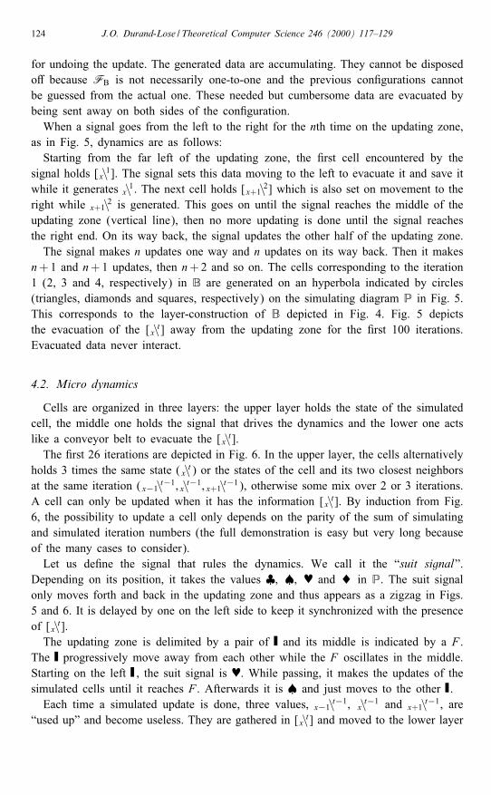
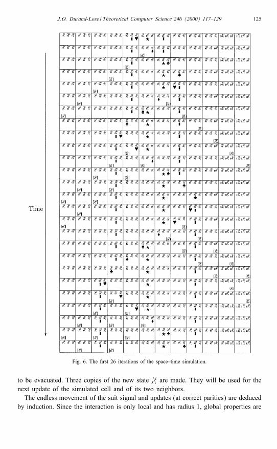
Cells are organized in three layers: the upper layer holds the state of the simulatedcell, the middle one holds the signal that drives the dynamics and the lower one actslike a conveyor belt to evacuate the [ x\t].The �rst 26 iterations are depicted in Fig. 6. In the upper layer, the cells alternatively

holds 3 times the same state ( x\t) or the states of the cell and its two closest neighborsat the same iteration ( x−1\t−1; x\t−1; x+1\t−1), otherwise some mix over 2 or 3 iterations.A cell can only be updated when it has the information [ x\t]. By induction from Fig.6, the possibility to update a cell only depends on the parity of the sum of simulatingand simulated iteration numbers (the full demonstration is easy but very long becauseof the many cases to consider).Let us de�ne the signal that rules the dynamics. We call it the “suit signal”.

Depending on its position, it takes the values ♣; ♠; $ and � in P. The suit signalonly moves forth and back in the updating zone and thus appears as a zigzag in Figs.5 and 6. It is delayed by one on the left side to keep it synchronized with the presenceof [ x\t].The updating zone is delimited by a pair of and its middle is indicated by a F .

The progressively move away from each other while the F oscillates in the middle.Starting on the left , the suit signal is $. While passing, it makes the updates of thesimulated cells until it reaches F . Afterwards it is ♠ and just moves to the other .Each time a simulated update is done, three values, x−1\t−1; x\t−1 and x+1\t−1, are

“used up” and become useless. They are gathered in [ x\t] and moved to the lower layer


Fig. 6. The �rst 26 iterations of the space–time simulation.

to be evacuated. Three copies of the new state x\t are made. They will be used for thenext update of the simulated cell and of its two neighbors.The endless movement of the suit signal and updates (at correct parities) are deduced

by induction. Since the interaction is only local and has radius 1, global properties are


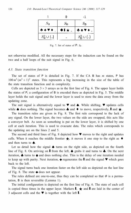
Fig. 7. Set of states of P: SP.

not otherwise modi�ed. All the necessary steps for the induction can be found on thetwo and a half loops of the suit signal in Fig. 6.

4.3. State transition function

The set of states of P is detailed in Fig. 7. If the CA B has m states, P has100m3 (m3 + 1)2 states. This represents a big increasing in the size of the table ofthe state transition function and in complexity.Cells are depicted as 3× 3 arrays as in the �rst line of Fig. 6. The upper layer holds

the states of P; a con�guration of B is encoded there as depicted in Fig. 5. The middlelayer holds the suit signal and the lower layer is used to store the data away from theupdating zone.The suit signal is alternatively equal to $ and ♠. While shifting, $ updates cells

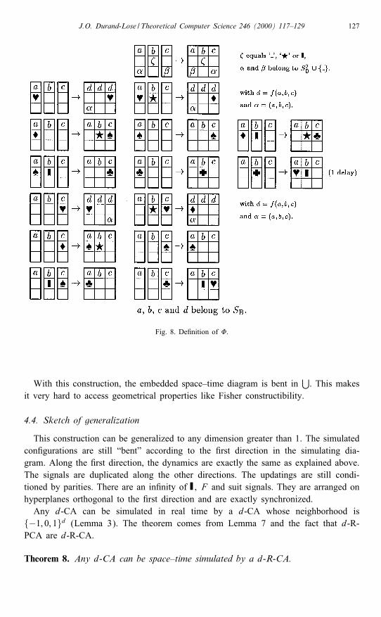
while ♠ does nothing. The signal becomes ♣ and � to move, respectively, and F.The transition rules are given in Fig. 8. The �rst rule correspond to the lack of

any signal. On the lower layer, the two values on the side are swapped, this acts likea conveyor belt. As soon as something is put on the lower layer, it is shifted by onecell at each iteration. This is used to evacuate data. The rules which corresponds tothe updating are on the lines 2 and 5.The second and third lines of Fig. 8 depicted how $ moves to the right and updates

cells. When it reaches the middle frontier F, it moves it one step to the right as �and then turns to ♠.Let us detail how the signal ♠ turns on the right side, as depicted on the fourth

line of Fig. 8. On arriving on from the left, ♠ grabs it and turns to ♣. On the nextiteration, ♣ turns to and does nothing else. This is the delay of one iteration neededto keep up with parity. Next iteration, regenerates the and the signal $ which goesback to the left.The signal turns back one iteration faster on the left side as depicted on the last line

of Fig. 8. The state does not appear.The rules de�ned are one-to-one, thus they can be completed so that � is a permu-

tation, B is then reversible (Lemma 1).The initial con�guration is depicted on the �rst line of Fig. 6. The state of each cell

is copied three times in the upper layer. Markers ; F and are laid in the center of3 adjacent cells and the $ is together with the left .


Fig. 8. De�nition of �.

With this construction, the embedded space–time diagram is bent in⋃. This makes

it very hard to access geometrical properties like Fisher constructibility.

4.4. Sketch of generalization

This construction can be generalized to any dimension greater than 1. The simulatedcon�gurations are still “bent” according to the �rst direction in the simulating dia-gram. Along the �rst direction, the dynamics are exactly the same as explained above.The signals are duplicated along the other directions. The updatings are still condi-tioned by parities. There are an in�nity of ; F and suit signals. They are arranged onhyperplanes orthogonal to the �rst direction and are exactly synchronized.Any d-CA can be simulated in real time by a d-CA whose neighborhood is

{−1; 0; 1}d (Lemma 3). The theorem comes from Lemma 7 and the fact that d-R-PCA are d-R-CA.

Theorem 8. Any d-CA can be space–time simulated by a d-R-CA.


There are d-R-CA able to simulate (iteratively) all d-R-CA over any con�guration[3].

Theorem 9. There are d-R-CA able to space–time simulate any d-CA.

5. Conclusion

With our space–time simulation, it is not possible to go backward before the �rst con-�guration if no previous con�guration were previously encoded in the initial con�gura-tion. Moreover, there is no guarantee that any previous con�guration doesexist.An in�nite time is required to fully generate the con�guration after one iteration.

When the signi�cant part of a con�guration represents only a �nite part of the space,the result of the computation is given in �nite time like in [11, 12].Although space–time simulation is an extension of iterative simulation, it di�ers. For

example, it keeps the locality of the information processing but is not shift invariant(at least in our construction).It would be interesting to know up to what extend the techniques and results of this

article can be adapted to the case where � is bounded when t is �xed. We believe thatit corresponds to an iterative simulation via some kind of grouping.

References

[1] S. Amoroso, Y. Patt, Decision procedure for surjectivity and injectivity of parallel maps for tessellationstructure, J. Comput. System Sci. 6 (1972) 448–464.

[2] J.O. Durand-Lose, Reversible cellular automaton able to simulate any other reversible one usingpartitioning automata, in: R. Baeza-Yates, E. Coles and P. Poblete, Eds., LATIN’95, Lecture notesin Computer Science, vol. 911, Springer, Berlin, 1995, pp. 230–244.

[3] J.O. Durand-Lose, Intrinsic universality of a one-dimensional reversible cellular automaton, in:R. Relschuk and M. Morvan, Eds., STACS’97, Lecture notes in Computer Science, vol. 1200, Springer,Berlin, 1997, pp. 439–450.

[4] P.C. Fisher, Generation of primes by a one-dimension real-time iterative array, J. ACM 12(3) (1965)388–394.

[5] G.A. Hedlund, Endomorphism and automorphism of the shift dynamical system, Math. System Theory3 (1969) 320–375.

[6] O. Heen, Linear speed-up for cellular automata synchronizers and applications, Theoret. Comput. Sci.188(1-2) (1997) 45–57.

[7] J. Kari, Reversibility of 2D cellular automata is undecidable, Physica D 45 (1990) 379–385.[8] J. Mazoyer, Signals in one dimensional cellular automata, Tech. Report 94-50, LIP, ENS Lyon, 46 all�ee

d’Italie, 69 364 Lyon 7, 1994.[9] J. Mazoyer, Computations on one dimensional arrays, Ann. Math. Artif. Intell. 16 (1996) 285–309.[10] E. Moore, Machine models of self-reproduction, Proc. Symp. on Applied Mathematics, vol. 14, 1962,

pp. 17–33.[11] K. Morita, Computation-universality of one-dimensional one-way reversible cellular automata, Inform.

Process. Lett. 42 (1992) 325–329.


[12] K. Morita, Reversible simulation of one-dimensional irreversible cellular automata, Theoret. Comput.Sci. 148 (1995) 157–163.

[13] J. Myhill, The converse of Moore’s garden-of-eden theorem, Proc. Symp. of Appl. Mathematics, no.14, 1963, pp. 685–686.

[14] D. Richardson, Tessellations with local transformations, J. Comput. System Sci. 6 (1972) 373–388.[15] T. To�oli, Computation and construction universality of reversible cellular automata, J. Comput. System

Sci. 15 (1977) 213–231.

reversible space–time simulation of cellular automata

Documents