reverse-engineering banks’ - rutgers...
TRANSCRIPT
R U T C O R R E S E A R C H R E P O R T
RUTCOR
Rutgers Center for
Operations Research
Rutgers University
640 Bartholomew Road
Piscataway, New Jersey
08854-8003
Telephone: 732-445-3804
Telefax: 732-445-5472
Email: [email protected]
http://rutcor.rutgers.edu/~rrr
REVERSE-ENGINEERING BANKS’ FINANCIAL STRENGTH RATINGS
USING LOGICAL ANALYSIS OF DATA
P.L. HAMMERa A. Koganb M.A. Lejeunec
RRR 10-2007, JANUARY 2007
a [email protected] , Tel.: +1 7324454812 ; Fax: +1 7324455472 b [email protected] c [email protected] a,b RUTCOR - Rutgers University Center for Operations Research, Piscataway, NJ, USA b Rutgers Business School, Rutgers University, Newark-New Brunswick, NJ, USA c Tepper School of Business, Carnegie Mellon University, Pittsburgh, PA, USA

RUTCOR RESEARCH REPORT RRR 10-2007, JANUARY 2007
REVERSE-ENGINEERING BANKS’ FINANCIAL STRENGTH RATINGS
USING LOGICAL ANALYSIS OF DATA
P.L. Hammer A. Kogan M.A. Lejeune
Abstract. We study the problem of evaluating the creditworthiness of banks using statistical, as well as combinatorics, optimization and logic-based methodologies. We reverse-engineer the Fitch credit risk ratings of banks using ordered logistic regression and Logical Analysis of Data (LAD). It is shown that LAD provides the most accurate rating model. The obtained ratings are successfully cross-validated, and the derived model is used to identify the financial variables most important for bank ratings. The study also shows that the LAD rating approach is (i) objective, (ii) transparent, (iii) generalizable. It can be used to develop internal rating systems that (iv) have varying levels of granularity, allowing their use at various stages in the credit granting decision process (pre-approval, determination of pricing policies), and (v) are Basel 2 compliant. Keywords: credit risk rating, bank creditworthiness, Logical Analysis of Data, combinatorial pattern extraction, Basel II

RRR 10-2007 PAGE 3
3
1 Credit Risk Ratings pf Banks and their Importance The internationalization of financial markets has significantly expanded investment
opportunities and risks. The need to obtain reliable and independent measures of creditworthiness has increased accordingly, and have led the rating industry (credit risk rating agencies such as Standard and Poor’s (S&P), Moody’s, Fitch and Euromoney) to expand the range of borrowers for which they provide risk opinion.
The importance of credit risk rating systems is manifold. First, the credit risk rating is assigned and used at the time the underwriting or credit approval decision is made, and a binary decision model is used to pre-approve the decision to grant or not the credit. Second, in case of pre-approval, the credit risk rating impacts the conditions (underwriting limits, maturity, interest rate, covenants, collaterals) under which the final approval can be given (Treacy and Carey, 2000). Such decisions can benefit from a more elaborate risk rating model, i.e. the one with more granularity. Third, the credit risk rating is a variable used for calculating the expected losses, which, in turn, are used to determine the amount of economic and regulatory capital a bank must keep to hedge against possible defaults of its borrowers. The expected loss of a credit facility is an increasing function of the probability of default of the borrower to which the credit line is granted, as well as the exposure-at-default and the loss given default associated with the credit facility. Since there is usually a mapping between credit risk rating and the borrower’s probability of default, and provided that the rating of a borrower is known to be a key predictor to assess the recovery rate associated with a credit facility granted to this borrower, the importance of the credit risk rating in calculating the amounts of regulatory and economic capital is evident.
Financial institutions, while taking into account external ratings (e.g., those provided by Fitch, Moody’s, S&P), have increasingly been developing efficient and refined internal rating systems over the past years. The reasons for this trend are manifold. First, the work of rating agencies, providing external, public ratings, has recently come under intense scrutiny and criticism, justified partly by their inability to spot some of the largest financial collapses of the decade (Enron Corp, WorldCom Inc). At his March 2006 testimony before the Senate Banking Committee, the president and CEO of the CFA Institute highlighted the conflicts of interest in credit ratings agencies (Wall Street Letter, 2006). He regretted that credit rating agencies "have been reluctant to embrace any type of regulation over the services they provide", and reported that credit rating agencies "should be held to the highest standards of transparency, disclosure and professional conduct. Instead, there are no standards". The reader is referred to Hammer et al. (2006) for a discussion of some specific criticisms against rating agencies.
Second, an internal rating system provides autonomy to a bank’s management in defining credit risk in line with that bank’s own core business and best international practices. Internal ratings are also used is reporting to senior management and trustees various key metrics such as risk positions, loan loss reserves, economic capital allocation, profitability, and employee compensation (Treacy and Carey, 2000).
Third, the New Basel Capital Accord (Basel II) requires banks to implement a robust framework for the evaluation of credit risk exposures that financial institutions face and the

PAGE 4 RRR 10-2007
capital requirements they must bear. While Basel Committee on Banking Supervision of the Bank for International Settlements favored originally (i.e., in the 1988 Capital Accord) the ratings provided by external credit ratings agencies, it is now encouraging the Internal Ratings-Based (IRB) approach under which banks use their own internal rating estimates to define and calculate default risk, on the condition that the robust regulatory standards are met and the internal rating system is validated by the national supervisory authorities. The committee has defined strict rules for credit risk models used by financial institutions, and requires them to develop and cross-validate these models (rating, probability of default, loss given default, exposure-at-default) in order to comply with the Basel II standard (Basel Committee on Banking Supervision, 1999, 2001, 2006).
Fourth, aside from the Basel II requirements, banks are developing internal risk models to make the evaluation of credit risk exposure more accurate and transparent. Credit policies and processes will be more efficient, and the quality of data will be improved. This is expected to translate into substantial savings on capital requirements. Today’s eight cents out of every dollar that banks hold in capital reserves could be reduced in banks with conservative credit risk policies, resulting in higher profitability.
The importance of evaluating the credit quality of banks has become more acute in the last 30 years in view of the increase in the number of bank failures, even in highly developed economies (Basel Committee on Banking Supervision, 2004). During the period from 1950 to 1980, bank failures averaged less than seven per year, whereas during the period from 1986 to 1991, they averaged 175 per year (Barr and Siems, 1994). Bank failures severely strain the Federal Deposit Insurance Corporation’s resources and undermine investor confidence. Curry and Shibut (2000) estimate that this so-called Savings and Loan crisis cost the U.S. taxpayers about $123.8 billion, 2.1% of 1990 GDP. Updated statistics of bank failure and default are provided by Fitch Ratings (2003). Central banks are afraid of widespread bank failures since they could exacerbate cyclical recessions and result in more severe financial crises (Basel Committee on Banking Supervision, 2004). More accurate credit risk models for banks could enable the identification of problematic banks early, which is seen as a necessary condition by the Bank of International Settlements (2004) to avoid failure, and could serve the regulators in their efforts to minimize bailout costs.
The evaluation and rating of the creditworthiness of banks and other financial organizations is particularly challenging, since banks and insurance companies appear to be more opaque than firms operating in other industrial sectors. Morgan (2002) attributes this to the fact that banks hold certain assets, such as loans and trading assets, the risks of which change easily and are very difficult to evaluate, and it is further compounded by banks' high leverage. Therefore, it is not surprising that the main rating agencies (Moody's and S&P) disagree much more often about the ratings given to banks than about those given to entities in other sectors. The difficulty and importance of accurately rating those organizations is also due the fact that the rating migration volatility of banks is historically significantly higher than it is for corporations and countries, and that banks tend to have higher default rates than corporations (de Servigny and Renault, 2004). Another distinguishing characteristic of the banking sector is the external support (i.e., from governments, etc.) that banks receive and the other corporate sectors do not (Fitch Rating, 2006). We provide below a brief review of the literature devoted to the rating and evaluation of credit risk of financial institutions.

RRR 10-2007 PAGE 5
5
Ronn and Vierma (1989) as well as Kiesel et al. (2001) examine the probability of a bank to default using respectively an equity-based model and a rating-based model. Barr and Siems (1994) use Data Envelopment Analysis (DEA) to predict bank failure using management quality measures as predictor. Estrella et al. (2002) compare the predictive power of the three basic ratios (leverage, gross revenue and assets) with that of bank credit risk ratings on bank failures.
A number of recent studies have also been conducted to identify predictive variables for bank performance, or to derive bank rating or classification systems. Considering East Asian economies during the years 1996-1998, Bongini et al. (2002) evaluate the predictive power of three sets of indicators (accounting data, stock market prices, and credit ratings) for determining the vulnerability of a bank. They show that credit rating agencies are not more predictive than backward-looking information contained in the balance sheet data, but that stock market-based information reflects more quickly the changing financial situation than credit risk ratings. They recommend the simultaneous use of several indicators for evaluating bank vulnerability, especially when dealing with banks in developing countries. van Soest et al. (2003) analyze existing bank ratings and compare them using ordered probit models, the independent variables of which include the size indicators and financial ratios characterizing profitability and default risk on loans. Analyzing a sample of 29 bank insolvencies, Caprio and Klingebiel (1996) identify macroeconomic (recession, terms of trade) and microeconomic (poor supervision, deficient bank management) variables important for explaining insolvencies of banks.
Poon et al. (1999) study the content of bank financial strength ratings (BFSR), published by Moody’s since 1995. Their dataset includes 130 banks located in 30 different countries, for which 100 bank-specific accounting and financial variables have been collected, reflecting profitability, efficiency, asset composition, interest composition, interest coverage, leverage, and risk. First, factor analysis is used to reduce the number of independent variables and to identify the critical constructs explaining BFSR. Three factors (FS1, FS2, FS3) accounting for more than 50% of the variability in the dataset are identified; these are seen as critical factors of a “bank’s intrinsic safety” (Poon et al., 1999). Based on the loadings of the original variables on the three identified factors, these latter ones are interpreted as: i) the dimension of risk, ii) the loan provision, and iii) the profitability. Second, several ordered logistic regression models are constructed, in which the independent variables are the scores of the three factors identified through factor analysis, the long-term debt rating (LTDR) and the short-term debt rating (STDR) of a bank, and the composite risk rating (CR) of the country where a bank is operating. Ranging from A to E+, Moody’s BFSRs are coded as ten ordinal values; Moody’s LTDRs are coded on a 21-point scale , while Moody’s STDRs are coded on a four-point scale in Poon et al.’s ordered logit model.
The general logistic model takes the following form 1 2 3 4 5 61 2 3Z FS FS FS STDR LTDR CRα β β β β β β ε= + + + + + + + , (1)
and the probability of a BFSR is written as:
1
z
z
epe
−
−=+
(2)
The different logistic models evaluated are reduced forms of (1): the multicolinearity between variables, in particular between STDR and LTDR, prevents the simultaneous inclusion of all the variables. The classification accuracy of these models varies significantly between 21.1

PAGE 6 RRR 10-2007
% and 71.1%. The best result is obtained when using the three factors and the LTDRs as independent variables. The country risk rating appears to have a very low predictive power.
Sarkar and Sriram (2001) develop a Bayesian model aimed at providing early warnings for bank failures and a supporting tool in the auditor’s judgment process. The model uses financial ratios as predictors of a bank’s performance to assess the posterior probability of a banks financial health (alternatively, financial distress). Studying the problem of predicting bank failure, Salchenberger et al. (1992), Tam and Kiang (1992) as well as Huang et al. (2004) found that neural network methods perform better than statistical ones (discriminant analysis, logistic regression). Huang et al. (2004) explain the lower accuracy of the statistical methods by the fact that the multivariate normality assumption for independent variables is very often violated in financial data sets. Huang et al. (2004) use a backpropagation neural network and a support vector machine to evaluate the creditworthiness of banks. They consider two different sets of banks located in the United States and in Taiwan. They observe that that the most important variables to predict banks’ creditworthiness differ for the two datasets. Total assets and total liabilities are the variables with the largest predictive power for the US banks, while operating profit margin is the key predictor for the Taiwanese banks.
Very recently, Fitch Ratings (2006) analyzed a bank rating method based on joint probability analysis, which includes as input variables the probability of the bank failing and the probability of the potential supporter (i.e., a sovereign state) defaulting at the same time, and, if there is no such simultaneous default, the probability of the supporter being willing or not to provide such support. Fitch Ratings comes to the conclusion that such a method is conceptually valid, but insists on the difficulty of constructing such a robust model, in view of the scarcity of the available empirical data.
2 Objectives and structure of the paper Information-intensive organizations such as banks have yet to find optimal ways to exploit
the increased availability of financial data (de Servigny and Renault, 2004, Wang and Weigend, 2004). Data mining and machine learning, in particular statistical (Jain et al,, 2000) and combinatorial pattern recognition (Hammer and Bonates, 2006), provide a wealth of opportunities for the credit rating and scoring field, which lags behind the state-of-the-art methodological developments (Galindo and Tamayo, 2000, de Servigny and Renault, 2004, Huang et al., 2004). In this paper, we use the novel combinatorial and logic-based techniques of Logical Analysis of Data (LAD) to develop credit risk rating models for evaluating the creditworthiness of banks.
The objective of this paper is to reverse-engineer the Fitch bank ratings to produce an (i) objective, (ii) transparent, (iii) accurate, and (iv) generalizable bank rating system. By the objectivity of a rating system we mean its reliance only on measurable characteristics of the rated banks. By its transparency we mean its formal explicit specification. By the accuracy of a rating system which is based on a widely used existing (proprietary and opaque) rating system we mean the close agreement of its ratings with those of the existing system. By its generalizability we mean its accuracy in rating those banks which were not used in developing the system. In this study, we shall:
RRR 10-2007 PAGE 7
7
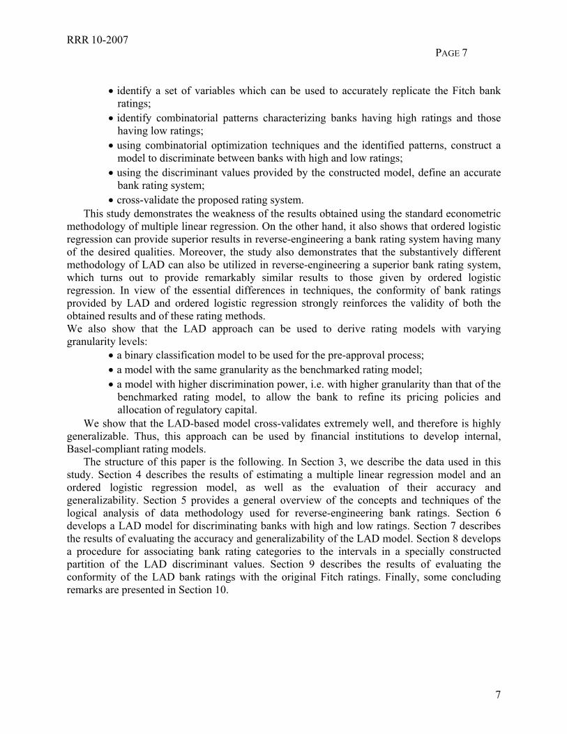
• identify a set of variables which can be used to accurately replicate the Fitch bank ratings;
• identify combinatorial patterns characterizing banks having high ratings and those having low ratings;
• using combinatorial optimization techniques and the identified patterns, construct a model to discriminate between banks with high and low ratings;
• using the discriminant values provided by the constructed model, define an accurate bank rating system;
• cross-validate the proposed rating system. This study demonstrates the weakness of the results obtained using the standard econometric
methodology of multiple linear regression. On the other hand, it also shows that ordered logistic regression can provide superior results in reverse-engineering a bank rating system having many of the desired qualities. Moreover, the study also demonstrates that the substantively different methodology of LAD can also be utilized in reverse-engineering a superior bank rating system, which turns out to provide remarkably similar results to those given by ordered logistic regression. In view of the essential differences in techniques, the conformity of bank ratings provided by LAD and ordered logistic regression strongly reinforces the validity of both the obtained results and of these rating methods. We also show that the LAD approach can be used to derive rating models with varying granularity levels:
• a binary classification model to be used for the pre-approval process; • a model with the same granularity as the benchmarked rating model; • a model with higher discrimination power, i.e. with higher granularity than that of the
benchmarked rating model, to allow the bank to refine its pricing policies and allocation of regulatory capital.
We show that the LAD-based model cross-validates extremely well, and therefore is highly generalizable. Thus, this approach can be used by financial institutions to develop internal, Basel-compliant rating models.
The structure of this paper is the following. In Section 3, we describe the data used in this study. Section 4 describes the results of estimating a multiple linear regression model and an ordered logistic regression model, as well as the evaluation of their accuracy and generalizability. Section 5 provides a general overview of the concepts and techniques of the logical analysis of data methodology used for reverse-engineering bank ratings. Section 6 develops a LAD model for discriminating banks with high and low ratings. Section 7 describes the results of evaluating the accuracy and generalizability of the LAD model. Section 8 develops a procedure for associating bank rating categories to the intervals in a specially constructed partition of the LAD discriminant values. Section 9 describes the results of evaluating the conformity of the LAD bank ratings with the original Fitch ratings. Finally, some concluding remarks are presented in Section 10.

PAGE 8 RRR 10-2007
3 Data
3.1 Ratings In this section, we shall briefly describe the Fitch Individual Bank rating system. After the
merger with Thomson BankWatch, Fitch has been publishing over 1,000 international bank ratings worldwide, and it is generally viewed as the leading agency for rating bank credit quality. Fitch provides long- and short-term credit ratings, which are viewed as an opinion on the ability of an entity to meet financial commitments (interest, preferred dividends, or repayment of principal) on a timely basis (Fitch Rating, 2001). These ratings are assigned to sovereigns and corporations, including banks, and are comparable worldwide.
Fitch provides a specialized rating scale for banks using individual and support ratings. Support ratings comprise 5 rating categories and assess the likelihood for a banking institution to receive support either from the owners or the governmental authorities should it run into difficulties. While the availability of support is a critical characteristic of a bank, it does not describe completely the banks’ solvability in case of adverse situations. It is worth noting for instance that even though a bank can have a state guarantee of support, its marketable obligations might drop. That is why, as a complement to a support rating, Fitch also provides an individual bank rating, which allows a credit quality evaluation separately from any consideration of outside support. It is purported to assess how a bank would be viewed if it were entirely independent and could not rely on external support. Factors such as profitability and balance sheet integrity, franchise, management, operating environment, and prospects, are therefore taken into consideration.
For banks in investment grade countries, support and individual bank rating scales provide sufficient scope for differentiation. However, the scope for differentiation between banks in non-investment grade countries can be more limited. Indeed, the rating of an obligor located in a given country is limited from above by the rating of that country (Ferri et al., 1999). In countries with weak country risk rating, it is thus possible that a number of banks’ ratings may be restricted by the sovereign’s foreign currency rating and will be bunched together at the sovereign ceiling. That is why national ratings were developed to provide a greater degree of differentiation between issuers and issues in countries where this bunching effect takes place. National ratings are an assessment of credit quality relative to the rating of the “best” credit risk in the country.
The national rating scale has 22 different risk categories as opposed to the 9 categories of the individual rating scale. Table 14 contains a detailed description of the rating categories characterizing the Fitch individual bank credit rating system. The individual bank credit ratings will be used in the remaining part of this paper, since these ratings are comparable across different countries, as contrasted with the national ratings, which are not.
3.2 Variables Based on the references mentioned in Section 1, approximately 40 parameters have been
provisionally considered as potentially significant predictors of the banks’ creditworthiness. After the elimination of those parameters for which not all the data were available, we have

RRR 10-2007 PAGE 9
9
restricted our attention to a set of 14 financial variables (loans, other earning assets, total earning assets, non-earning assets, net interest revenue, customer and short-term funding, overheads, equity, net income, total liability and equity, operating income) and 9 representative financial ratios. These ratios are defined in the Appendix and describe:
• asset quality: ratio of equity to total assets; • operations: net interest margin; ratio of interest income to average assets; ratio of
other operating income to average assets; ratio of non-interest expenses to average assets; return on average assets (ROAA); return on average equity (ROAE); cost to income ratio;
• liquidity: ratio of net loans to total assets. The values of these variables were collected at the end of 2000 and are disclosed in the
database called Bankscope, which is the largest existing bank database. Fitch Ratings has partnered with a Belgian electronic publishing firm, Bureau van Dijk, to provide clients with financial statement data on more than 11,000 banks worldwide .
As an additional variable, we use in this study the S&P risk rating of the country where the bank is located. The S&P country risk rating scale comprises twenty-two different categories (from AAA to D). We convert these categorical ratings into a numerical scale, assigning the largest numerical value (21) to the countries with the highest rating (AAA). Similar numerical conversions of country risk ratings are also used by Bouchet et al. (2003), Ferri et al.(1999), Monfort and Mulder (2000), Mulder and Perelli (2001), and Sy (2003). Moreover, Bloomberg, a major provider of financial data services, developed a standard cardinal scale for comparing Moody’s, S&P and Fitch-BCA ratings (Kaminsky and Schmukler, 2002).
3.3 Observations Our dataset consists of eight hundred banks rated by Fitch and operating in 70 different
countries. Table 1 provides the geographic distribution of the banks included in the dataset.
Table 2 lists the number and percentage of the banks in the dataset in each rating category. It can be seen that the extremal rating categories (A and E) comprise a very small number of banks (19 and 32 respectively). The majority of the banks contained in the dataset have received intermediate ratings.

PAGE 10 RRR 10-2007
Table 1 : Geographic Distribution of Banks
Origin Number of banks Countries
Western Europe 247
Andorra (3), Austria (1), Belgium (8), Denmark (4), Finland (4), France (29), Germany (31), Greece (5), Iceland (2), Ireland (5), Italy (30), Luxembourg (2), The Netherlands (12), Norway (9), Portugal (10), Spain (42), Sweden (6), Switzerland (5), UK (39)
Eastern Europe 51
Croatia (2), Czech Republic (3), Hungary (3), Latvia (1), Lithuania (4), Poland (7), , Romania (2), Russia (19), Slovak Republic (3), Slovenia (6), Ukraine (2)
Canada and USA 198 Canada (6), USA (192)
Developing Latin American countries 45
Argentina (2), Bermuda (2), Brazil (10), Chile (5), Colombia (2), Dominican Republic (4), El Salvador (2), Mexico (6), Panama (2), Peru (1), Venezuela (9)
Middle East 44 Bahrain (5), Cyprus (2), Egypt (2), Kuwait (4), Lebanon (2), Malta (1), Saudi Arabia (8), Turkey (14), United Arab Emirates (6)
Hong-Kong, Japan, Singapore 55 Hong-Kong (18), Japan (34), Singapore (3)
Developing Asian countries 145
Azerbaijan (1), China (16), India (32), Indonesia (9), Kazakhstan (5), South Korea (12), Malaysia (8), Pakistan (4), Philippines (14), Taiwan (31), Thailand (10), Vietnam (3)
Oceania 6 Australia (6) Africa 6 South Africa (6) Israel 3 Israel (3)
Table 2 : Distribution of Banks in Rating Categories
Rating Categories Number of Banks Percentage A 19 2.375%
A/B 60 7.500% B 203 25.375%
B/C 129 16.125% C 121 15.125%
C/D 77 9.625% D 93 11.625%
D/E 66 8.250% E 32 4.000%

RRR 10-2007 PAGE 11
11
4 Regression models The first issue to address in reverse-engineering a bank rating system concerns the choice of
explanatory variables to be used in constructing the model. More precisely, the question to be answered is whether the amount of information contained in the selected set of 24 variables is sufficient for correctly classifying the 800 banks in the dataset. We shall provide below an affirmative answer to this question. Moreover, the model constructed in this section will serve later as a benchmark to evaluate the qualities of other rating models.
4.1 Multiple linear regression model The standard econometric technique of multiple linear regression can be used to model the
dependency of bank ratings on the independent variables described in the previous section. In this model, the dependent variable y is the numerical scale of the Fitch individual bank ratings as presented in Table 14. The 24 independent variables described in the previous section are denoted by x1,…,x24. The estimation of the standard regression model
24
1 i i
iy a xβ ε
=
= + +∑ (3)
gives the results shown in Table 15. It can be seen that while the regression model is statistically significant, its goodness-of-fit as
measured by the R-square is equal to only 54.9%, which is not sufficiently high to be used as an accurate model of bank ratings.
To assess the generalizability and predictive value of the regression model, we shall use the technique of 2-fold cross-validation (see e.g., Hjorth, 1994), i.e., we randomly partition the set of 800 banks into 2 disjoint subsets of 400 banks each. First, we remove one of the subsets, estimate the regression model on the remaining 50% of the data, and then evaluate the R-square of the estimated regression model on the removed subset. Then we reverse the role of the two subsets, repeat the calculations, and calculate the average of the two R-squares. Finally, the 2-fold cross-validation process is repeated 10 times, using each time another randomly generated equipartition of the dataset. The average R-square obtained in these 10 2-fold cross-validation experiments turns out to be 0.5161 with the standard deviation of 0.145. The results above show that while the regression model does not seem to be overfitting the data, it has only a limited generalizability. This negative conclusion is very much in agreement with Morgan’s (2002) observations according to which the main rating agencies have serious difficulties in evaluating the ratings of banks and insurance companies, as manifested in the frequency of their divergent evaluations.
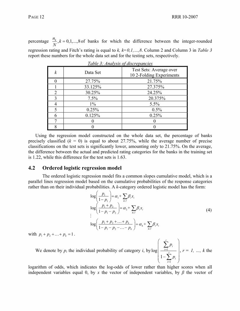
Denoting by ŷj bank j’s rating predicted using the regression model, by jy the rounding of ŷj to its closest integer value and by rj the rating given by Fitch to bank j, we compute the difference dj between the rounded regression rating and Fitch’s rating: dj =|ŷ−rj|, j N∈ . Now we can calculate { | , } , 0,1,...,8k jn j d k j N k= = ∈ = , where nk, called the discrepancy count, represents the number of banks whose integer-rounded rating category predicted by a rating model differs from the actual Fitch rating by exactly k categories. In Table 3, we report the
PAGE 12 RRR 10-2007
percentage , 0,1,...,8kn kN
= of banks for which the difference between the integer-rounded
regression rating and Fitch’s rating is equal to k, k=0,1,…,8. Column 2 and Column 3 in Table 3 report these numbers for the whole data set and for the testing sets, respectively.
Table 3: Analysis of discrepancies
k Data Set Test Sets: Average over 10 2-Folding Experiments
0 27.75% 21.75% 1 33.125% 27.375% 2 30.25% 24.25% 3 7.5% 20.375% 4 1% 5.5% 5 0.25% 0.5% 6 0.125% 0.25% 7 0 0 8 0 0
Using the regression model constructed on the whole data set, the percentage of banks precisely classified (k = 0) is equal to about 27.75%, while the average number of precise classifications on the test sets is significantly lower, amounting only to 21.75%. On the average, the difference between the actual and predicted rating categories for the banks in the training set is 1.22, while this difference for the test sets is 1.63.
4.2 Ordered logistic regression model The ordered logistic regression model fits a common slopes cumulative model, which is a
parallel lines regression model based on the cumulative probabilities of the response categories rather than on their individual probabilities. A k-category ordered logistic model has the form:
11
1
1 22
1 2
1 2
1 2
log + 1
log + 1
log + 1
i ii I
i ii I
kk i i
i Ik
p xp
p p xp p
p p p xp p p
α β
α β
α β
∈
∈
∈
= −
+= − −
+ + += − − − −
∑
∑
∑M
K
K
(4)
with 1 2 1kp p p+ + + =K .
We denote by pi the individual probability of category i, by 1
1
log1
r
ii
r
ii
p
p
=
=
−
∑
∑, r = 1, …, k the
logarithm of odds, which indicates the log-odds of lower rather than higher scores when all independent variables equal 0, by x the vector of independent variables, by β the vector of

RRR 10-2007 PAGE 13
13
logistic coefficients (slope parameters) that are category-invariant, and by αj the intercepts which are category-specific and satisfy the constraints:
1 2 1 k kα α α α−≤ ≤ ≤ ≤K . (5) Like dichotomous logistic regression, an ordered logistic regression model is estimated using maximum likelihood methods, to find the best set of regression coefficients to predict the values of the logit-transformed probability that the dependent variable falls into one category rather than another. Logistic regression assumes that if the fitted probability p is greater than 0.5, the dependent variable should have the value 1 rather than 0. Ordered logit doesn't have such a fixed assumption; it does instead fit a set of cutoff points. If there are (k+1) categories associated with the dependent variable, it will find k cutoff values r1 to rk such that if the fitted value of logit(p) is below r1, the dependent variable is predicted to take value 0, if the fitted value of logit(p) is between r1 and r2, the dependent variable is predicted to take value 1, and so on.
The most useful tool to assess the quality of the constructed ordered logistic regression model is by comparing actual group membership with the membership predicted by the model, as summarized in the analysis of discrepancies table. Below, we provide the analysis of discrepancies for the problem at hand, in which we have 9 discrepancy levels (k=0,1,…,8) and 24 independent variables (i=1,…,24). As we did above for the linear regression model, we apply the technique of 2-fold cross-validation, and repeat it 10 times.
Table 4: Analysis of discrepancies
k Data Set Test Sets: Average over 10 2-Folding Experiments
0 36.88% 30.75% 1 37.38% 38.375% 2 17.00% 17.25% 3 6.00% 8.375% 4 2.13% 3.5% 5 0.25% 0.475% 6 0.38% 0.25% 7 0% 0 8 0% 0
It can be seen in Table 4 that the percentage of banks precisely classified (k = 0) with the ordered logistic model built using the entire data set is equal to about 37%, while the average number of precise classifications on the test sets is lower, amounting to almost 31%. On the average, the difference between the actual and predicted rating categories for the banks in the data set is 1.04, while this difference for the test sets is 1.16. The Spearman rank correlation between the ordered logistic regression ratings and the Fitch ratings is equal to 75.60%.
Clearly, the ratings provided by this model are of good quality, thus proving the appropriateness of the selected set of 24 variables for the rating of bank creditworthiness. In the next sections, we shall describe a new type of rating model in which the rating of each bank is accompanied by a justification of why this bank has not been given a higher or a lower rating. Before constructing this new model, we shall briefly outline the “logical analysis of data” methodology on which this rating model will be based.

PAGE 14 RRR 10-2007
5 Logical Analysis of Data - An overview The logical analysis of data (LAD) is a combinatorics-, optimization-, and Boolean logic-
based methodology for analyzing archives of observations. Initially created for the classification of binary data (Hammer 1986, Crama et al., 1988), LAD was later extended (Boros et al., 1997) from datasets having only binary variables to datasets which contain numerical variables. LAD distinguishes itself from other classification methods and data mining algorithms by the fact that it generates and analyzes exhaustively a major subset of those combinations of variables which can describe the positive or negative nature of observations (e.g. to describe solvent or insolvent banks, healthy or sick patients, etc.), and uses optimization techniques to extract models constructed with the help of a limited number of significant combinatorial patterns generated in this way (Boros et al., 2000).
We shall sketch below very briefly the basic concepts of LAD, referring the reader for a more detailed description to Crama et al. [1988], or Boros et al. [2000], or to the recent survey (Hammer and Bonates, 2005).
In LAD, as in most of the other data analysis methods, each observation is assumed to be represented by an n-dimensional real-valued vector. For the observations in the given dataset, beside the values of the n components of this vector, an additional binary (0, 1) value is also specified; this additional value is called the output or the class of the observation, with the convention that 0 is associated to negative observations, and 1 to the positive ones.
The purpose of LAD is to discover a binary-valued function f depending on the n input variables, which provides a discrimination between positive and negative observations, and which closely approximates the actual one. This function f is constructed as a weighed sum of patterns.
In order to clarify how such a function f is found we shall start by transforming the original dataset to one in which the variables can only take the values 0 and 1. We shall achieve this goal by using indicator variables which show whether the values the variables take in a particular observation are “large” or “small”; more precisely, each indicator variable shows whether the value of a numerical variable does or does not exceed a specified level, called a cutpoint. For example, to the numerical variable ratio of costs to incomes, we shall associate in our banking model an indicator variable showing whether the pretax profits did or did not exceed 71.92. The selection of the cutpoints is achieved by solving an associated set covering problem (Boros et al., 1997). By associating an indicator variable to each cutpoint, the dataset is binarized. Positive (negative) patterns are combinatorial rules which impose upper and lower bounds on the values of a subset of input variables, such that:
• a sufficiently high proportion of the positive (negative) observations in the dataset satisfy the conditions imposed by the pattern, and
• a sufficiently high proportion of the negative (positive) observations violate at least one of the conditions of the pattern.
In order to give an example of a pattern in the bank rating dataset, let us first define as positive those banks whose ratings are B or higher, and as negative those banks whose ratings are D or lower. As an example of a positive pattern in our dataset, we mention the pattern requiring the simultaneous fulfillment of the following three conditions:

RRR 10-2007 PAGE 15
15
• the country risk rating is A+, AA-, AA, AA+, AAA, • the ratio of the costs to incomes is at most equal to 71.92, and • the return on equity is strictly larger than 11.8165%.
It can be seen that these three conditions are satisfied by 70.57% of the banks with ratings of B or higher, and by none of the banks rated D, D/E or E.
The following terminology will be useful throughout this paper. The degree of a pattern is the number of variables the values of which are bounded in the definition of the pattern. The prevalence of a positive (negative) pattern is the proportion of positive (negative) observations covered by it. The homogeneity of a positive (negative) pattern is the proportion of positive (negative) observations among those covered by it. The pattern in the above example has degree 3, prevalence 70.57% and homogeneity of 100%. Patterns of low degree, high prevalence and high homogeneity have been shown to be the most effective in LAD applications, e.g., (Boros et al., 2000).
The first step in applying LAD to a dataset is to generate the pandect, i.e., the collection of all patterns in a dataset. The number of patterns contained in the pandect of a dataset of such dimensions can be exponentially large, in the order of hundreds of thousands, possibly millions. Because of the enormous redundancy in this set, we shall impose a number of limitations on the set of patterns to be generated, by restricting their degrees (to low values), their prevalence (to high values), and their homogeneity (to high values); these bounds are known as LAD control parameters. It should be added that the quality of patterns satisfying these conditions is usually much higher than that of patterns having high degrees, or low prevalence, or low homogeneity. Several algorithms have been developed for the efficient generation of large subsets of the pandect corresponding to reasonable values of the control parameters (Alexe and Hammer 2005).
The substantial redundancy among the patterns of the pandect makes necessary the extraction of (relatively small) subsets of positive and negative patterns, sufficient for classifying the observations in the dataset. Such collections of positive and negative patterns are called models. A model is supposed to include sufficiently many positive (negative) patterns to guarantee that each of the positive (negative) observations in the dataset is “covered” by (i.e., satisfies the conditions of) at least one of the positive (negative) patterns in the model. Furthermore, good models tend to minimize the number of points in the dataset covered simultaneously by both positive and negative patterns in the model. It will be seen in the next section that the model we have found for the bank rating problem consists of 6 positive and 7 negative patterns, and that every negative or positive observation in the model is covered by some of the positive, respectively negative, patterns included in the model.
A LAD model can be used for classification in the following way. An observation (whether it is contained or not in the given dataset) which satisfies the conditions of some of the positive (negative) patterns in the model, but which does not satisfy the conditions of any of the negative (positive) patterns in the model, is classified as positive (negative).
An observation satisfying both positive and negative patterns in the model is classified with the help of a discriminant that assigns specific weights to the patterns in the model (Boros et al., 2000). More precisely, if p and q represent the number of positive and negative patterns in a model, and if h and k represent the numbers of those positive, respectively negative patterns in the model which cover a new observation ω, then the value of the discriminant ∆(ω) is simply

PAGE 16 RRR 10-2007
∆(ω) = h/p –k/q (6) and the corresponding classification is determined by the sign of this expression. Finally, an observation for which ∆(ω) = 0 is left unclassified, since the model either does not provide enough evidence, or provides conflicting evidence for its classification. Fortunately it has been seen in all the real-life problems considered that the number of unclassified observations is extremely small (usually less than 1%). We represent the results of classifying the set of all observations in a dataset in the form of a classification matrix (Table 5).
Table 5: Classification Matrix
Classification of Observations Observation Classes Positive Negative Unclassified Positive A c E Negative B d F
Here, the value a (respectively d) represents the percentage of positive (negative) observations that are correctly classified. The value c (respectively b) is the percentage of positive (negative) observations that are misclassified. The value e (respectively f) represents the percentage of positive (negative) observations that remain unclassified. Clearly, a+c+e=100% and b+d+f=100%. The quality of the classification is defined by:
Q = 12 [(a + d) + 1
2 (e+f)]. (7)
6 A LAD model for bank ratings
Since LAD is a classification methodology, it is natural to first associate to the bank rating problem a related classification problem, with the expectation that the resulting LAD model can be successfully utilized for establishing an objective and transparent bank rating system. We recall that we have defined as positive observations the banks which have been rated by Fitch as A, A/B or B, and as negative observations those whose Fitch rating is of D, D/E or E.
In the binarization process, cutpoints were introduced for the 19 of the 24 numerical variables shown in Table 6. Actually, the other 5 numerical variables (loans, total earning assets, total liabilities and equity, equity and net interest revenue), had been binarized also, but since it turned out that they were redundant, only the variables shown in Table 6 were retained for constructing the model. Table 6 provides all the cutpoints that were used in pattern and model construction. For example, two cutpoints (24.8 and 111.97) are used to binarize the numerical variable “Profit before Tax” (PbT), i.e., two binary indicator variables replace PbT, one telling whether PbT exceeds 24.8, and the other telling whether PbT exceeds 111.97.

RRR 10-2007 PAGE 17
17
Table 6: Cutpoints
Numerical Variables Cutpoints Numerical
Variables Cutpoints Numerical Variables Cutpoints
Country Risk Rating
11 , 16 , 19.5 , 20 Overhead 127, 324 Non Int Exp /
Avg Assets 2.00 , 2.77 , 3.71 , 4.93
Other Earning Assets
3809 , 9564.9 Profit before Tax 24.8 ,
111.97 Return on
Average Assets 0.30 , 0.80 ,
1.52 Non-Earning
Assets 364 Operating Income (Memo) 1360.74 Return on
Average Equity 11.82 , 15.85 ,
19.23
Total Assets 5735.8 Equity / Total Assets 4.90 Cost to Income
Ratio 50.76 , 71.92
Customer & Short Term
Funding
4151.3 , 9643.8
Net Interest Margin 1.87
Net Loans / Total Assets
44.95 , 53.90 , 59.67 , 66.50
Equity 370.45 Net Int Rev / Avg Assets 3.02
Other Operating
Income
46.8 , 155.5 , 470.5
Oth Op Inc / Avg Assets
0.83 , 1.28 , 1.86 , 3.10
The first step of applying the LAD technique to the problem binarized with the help of these variable cutpoints was the identification of a collection of powerful patterns. One example of such a powerful positive pattern was shown in the previous section. As an example of a powerful negative pattern, consider the pattern defined by the following two conditions
• the country risk rating is strictly lower than A, and • the profits before tax are at most equal to €111.96 millions.
One can see that these conditions describe a negative pattern, since none of the positive observations (i.e. banks rated A, A/B or B) satisfy both of them, while no less than 69.11% of the negative observations (i.e. those banks rated D, D/E or E) do satisfy both conditions. This pattern has degree 2, prevalence 69.11%, and homogeneity 100% (since none of the positive observations satisfy its defining conditions).
The model we have developed for bank ratings, shown in Table 16, is very parsimonious, consisting of only eleven positive and eleven negative patterns (P1,…, P11, respectively, N1,…,N11), and is built on a support set of only 19 out of the 24 original variables. All the patterns in the model are of degree at most 3, have perfect homogeneity (100%), and very substantial prevalence (averaging 50.9% for the positive, and 37.7% for the negative patterns).
While the focus in LAD is on discovering how the interactions between the values of small groups of variables (as expressed in patterns) affect the outcome (i.e., the bank ratings), one can also use the LAD model to learn about the importance of individual variables. A natural measure of importance of a variable in an LAD model is the frequency of its appearance in the model’s patterns. The three most important variables in the 22 patterns constituting the LAD model are the credit risk rating of the country where the bank is located, the return on average total assets, and the return on average equity. The importance of the country risk rating variable, which appears in 18 of the 22 patterns, can be explained by the fact that credit rating agencies are often reluctant to give an entity a better credit risk rating than that of the country where it is located (Erb et al., 1996). This is why the country risk rating is sometimes referred to as the “sovereign ceiling” or the

PAGE 18 RRR 10-2007
“pivot of all other country’s ratings” (Ferri et al., 1999). The country risk rating was also found to be an important predictive variable for bank ratings by Poon et al. (1999). Both the return on average assets and the return on average equity variables appear in six patterns. These two ratios, respectively representing the efficiency of assets in generating profits, and that of shareholders' equity in generating profits, are critical indicators of a company’s prosperity, and are presented by Sarkar and Sriram (2001) as key predictors auditors use to evaluate the wealth of a bank. The return on average equity is also found significant for predicting the rating of US banks only by Huang et al. (2004).
7 Accuracy and Robustness of the LAD MODEL
Applying the LAD model described in the previous section to the classification of all the 473 banks whose ratings are A, A/B, B, D, D/E or E, we find the accuracy of the model to be 100%. In order to cross-validate the model’s accuracy, we have used 10 two-folding cross-validation experiments; in each two-folding cross validation experiment, the observations are randomly split into two approximately equal subsets, a model is constructed using one of the two subsets of observations, and it is applied for classifying the observations in the other subset. In the second half of the experiment, the roles of the two subsets are reversed, i.e. the set formerly used for testing is now used for training, and the one formerly used for training becomes the test set. The average accuracy of the 20 models obtained in this way was found to be 95.12%. It is remarkable that the standard deviation in the 20 experiments was only 0.03. The high accuracy and low standard deviation indicate high predictive value and the robustness of the proposed classification system.
As a second measure of accuracy of the model, we have examined the correlation between the values of the discriminant of the model (ranging between -1 and +1) and the bank ratings (represented on their numerical scale). Although this experiment included all the banks in the dataset (i.e., not only those rated A, A/B, B, D, D/E or E, which were used in creating the LAD model, but also those rated B/C, C or C/D, which were not used at all in the learning process), the correlation turned out to be of 80.70% -- reconfirming the high predictive value of the LAD model. We have also evaluated the stability of the correlation coefficient between the LAD discriminant values and the bank ratings, using the results of the two-fold cross-validation experiments described above. The average value of the correlation coefficient was found to be 80.04%, with standard deviation of 0.04, showing the stability of the close association between the values of the LAD discriminant and the original bank ratings.
Finally, as an additional check, we have separately calculated the average discriminant values for the nine rating categories. The results are presented in Table 7, and show clearly the discriminating power of the LAD model. Two interesting conclusions one can derive from this table are the following:
• The positive observations have higher average discriminant values than the unclassified ones, which in their turn have higher average discriminant values than the negative observations.
• The average discriminant values are monotonically decreasing with the rating categories. Moreover, although the model was not “taught” to make distinctions

RRR 10-2007 PAGE 19
19
between the categories A, A/B and B (and similarly between D, D/E and E), the average discriminant values drop by more than 10% from one category to the next.
• Even in the case of the “unclassified” observations, which were not used in deriving the LAD model, the average discriminant value for category C is lower than that for category B/C, and that for category C/D is higher than that of category D.
Table 7: Average Discriminant Values
Observation Class Rating Category
Discriminant Values / Category Averages
Discriminant Values / Class Weighted Averages
A 0.589 A/B 0.531 Positive B 0.495
0.538
B/C 0.209 C -0.004 Unclassified
C/D -0.156 0.016
D -0.357 D/E -0.378 Negative E -0.383
-0.380
8 From LAD discriminant values to ratings
In order to map the numerical values of the LAD discriminant to the nine bank rating categories of Fitch (A, A/B, …, E), we shall attempt to partition the interval of the discriminant values into nine sub-intervals corresponding to the nine categories. We shall assume that this partitioning is defined by cutpoints xi such that
-1 = x0 ≤ x1 ≤ x2≤ ……… ≤ x8 ≤ x9 = 1 ,
where i indexes the rating categories (with 1 corresponding to E, and 9 corresponding to A). Ideally, a bank should be rated i if its discriminant value falls between xi and xi+1 (e.g., it should be rated A if its value falls between x8 and x9).
In reality, such a partitioning may not exist. Therefore, in order to take “noisiness” into account, we shall replace the LAD discriminant values di of bank i by an adjusted discriminant value δi, and find values of δi for which such a partitioning exists, and which are “as close as possible” to the values di. As it is often the case, we interpret “as close as possible” as minimizing the mean square approximation error. If we denote by j(i) the rating category of bank i and by N the set of banks considered, then the determination of the cutpoints xj and of the adjusted discriminant values δi can be modeled as follows:

PAGE 20 RRR 10-2007
2
( ) 1
( )
0 1 2 8 9
( )
,,
1 ,..., ,..., 11 1,
i ii N
i j i
j i i
j
i
Minimize
d
subject to x i N
x i N
x x x x x x
i N
δ
δ
δ
δ
∈
+
−
≤ ∈
< ∈
− = ≤ ≤ ≤ ≤ =
− ≤ ≤ ∈
∑
(8)
To solve the convex nonlinear problem above, we use in our numerical experiments the NLP solvers LOQO and Lancelot, which are publicly available on the NEOS1 server (Czyzyk et al., 1998). The approach described above is very similar to the convex cost closure problem (Hochbaum and Queyranne 2003, Hochbaum 2004) that can be used to determine adjustments of the observations minimizing the value of the deviation penalty function, while satisfying the ranking order constraints.
The LAD discriminant derived above and the values of the cutpoints xi determined by solving problem (8) can be used not only for rating banks which are in the training sample, but even those which are not. In this case, the bank rating is determined by the particular sub-interval containing the LAD discriminant value. The values of the cutpoints xi determined by solving the problem (8) for all the 800 banks in the dataset are presented in Table 8.
Table 8 : Rating cutpoints
I 0 1 2 3 4 5 6 7 8 9 xi -1 -0.8100 -0.4025 -0.2850 -0.1150 0.0886 0.3306 0.6331 0.8250 1
As shown above, both LAD and ordered logistic regression can be successfully applied to derive a rating model which comprises the same number of categories as the benchmarked (i.e., Fitch) rating model. As compared to ordered logistic regression, the LAD-based approach has the additional advantage that it can be used for generating any required number of rating categories. The LAD-based rating model can take the form of a binary classification model, and can be used at the pre-approval stage to discriminate banks to which a credit line cannot be extended from those to which the granting of credit can be considered. The LAD rating approach can also be used to derive models with higher granularity (i.e., more than 9 rating categories), which are used by banks to further differentiate their customers and to tailor accordingly their credit pricing policies.
9 Conformity of Fitch and LAD Bank Ratings
In order to evaluate how well the original LAD discriminant values fit in the identified rating sub-intervals, we use the original (unadjusted) LAD discriminant value of each bank to determine its rating category. We recall that nk (k = 0,…,8) represent the number of banks whose
1 http://www-neos.mcs.anl.gov/

RRR 10-2007 PAGE 21
21
rating category determined in this way differs from the actual Fitch rating by exactly k categories, indicating the goodness-of-fit of the proposed rating system.
While the rating cutpoints were determined using all the banks in the sample, the LAD discriminant was derived only from the banks rated A, A/B, B, D, D/E and E. Therefore, the discrepancy counts should be calculated separately for the banks rated A, A/B, B, D, D/E and E, and for the banks rated B/C, C and C/D.
Table 9 : Discrepancy analysis
N = {A, A/B, B, D, D/E, E} N = {B/C, C, C/D} N = {A, A/B, B, B/C, C, C/D, D, D/E, E}k nk nk/|N| nk nk/|N| nk nk/|N| 0 140 29.60% 96 29.36% 236 29.50% 1 252 53.28% 156 47.71% 408 51.00% 2 57 12.05% 62 18.96% 119 14.88% 3 20 4.23% 11 3.36% 31 3.88% 4 4 0.85% 2 0.61% 6 0.75% 5 0 0.00% 0 0.00% 0 0.00% 6 0 0.00% 0 0.00% 0 0.00% 7 0 0.00% 0 0.00% 0 0.00% 8 0 0.00% 0 0.00% 0 0.00%
The discrepancy summary presented in Table 9 demonstrates a high goodness-of-fit of the proposed model. More than 95% of the banks are rated within at most two categories of their actual Fitch rating, with about 30% of the banks receiving exactly the same rating as in the Fitch rating system, and another 51% being off by exactly one rating category. The simplest reflection of the very high degree of coincidence between the LAD and the Fitch ratings is the fact that the weighted average distances between the two ratings are
• 0.93 for the categories A, A/B, B, D, D/E and E, • 0.98 for the categories B/C, C and C/D, and • 0.95 for all banks in the sample (categories A, A/B, B, B/C, C, C/D, D, D/E, E).
It is interesting to remark that the goodness-of-fit of the ratings calculated separately for the banks rated by Fitch as B/C, C and C/D (i.e., those banks which were not used in deriving the LAD model) is very close to the goodness-of-fit for the banks actually used (i.e. those rated by Fitch as A, A/B, B, D, D/E and E) for deriving the LAD model. This finding indicates the stability of the proposed rating system and its appropriateness for rating “new” banks, i.e. banks which are not rated by agencies or banks the rater has not dealt with before. The Spearman rank correlation between the LAD and the Fitch ratings is equal to 83.44%, and is higher than that between the ordered logistic regression ratings and the Fitch ones (75.60%).
In order to systematically evaluate the robustness of the proposed rating system, we shall use again the cross-validation technique described in Section 3. We shall apply 10 times the two-folding procedure to derive the average discrepancy counts of the bank ratings predicted for the testing sets. More specifically, in each two-folding experiment, those banks in the training set which are rated A, A/B, B, C/D, D, D/E are used to derive a LAD model. Then all the banks of the training set (including those rated B/C, C and C/D) are used to determine with the help of the

PAGE 22 RRR 10-2007
convex optimization problem (9) the rating cutpoints. Finally, the derived LAD model and the intervals determined by these rating cutpoints are used to determine ratings for the banks in the testing set. The accuracy of this rating is then evaluated using the discrepancy counts. The average discrepancy counts (over the two folds) for each of the 10 cross-validation runs are presented in Table 10, along with the average discrepancy counts over all the 10 experiments.
The fact that on the average -- if we include in our calculation every category of banks in the sample, whether it was used or not in deriving the LAD model – the difference between the Fitch and the LAD ratings is only 0.98, is an extremely strong indicator of the LAD model’s stability and the absence of overfitting. This result is particularly significant in view of the occasional reports in the financial data mining literature that the high fit of machine learning methods such as support vector machine as achieved at the risk of overfitting (Huang et al, 2004, Galindo and Tamido, 2000). Clearly, the LAD-based combinatorial rating approach presented in this paper is not subject to this overfitting problem.
Table 10 : Cross-validated discrepancy analysis
K Exp 1 nk/|N|
Exp 2 nk/|N|
Exp 3 nk/|N|
Exp 4 nk/|N|
Exp 5 nk/|N|
Exp 6 nk/|N|
Exp 7 nk/|N|
Exp 8 nk/|N|
Exp 9 nk/|N|
Exp 10 nk/|N|
Average nk/|N|
0 0.2775 0.3025 0.2925 0.2875 0.2825 0.305 0.2875 0.28 0.28875 0.2975 29.01% 1 0.545 0.515 0.495 0.485 0.52375 0.505 0.515 0.4975 0.50375 0.5325 51.18% 2 0.125 0.125 0.125 0.17125 0.15625 0.135 0.1425 0.13875 0.15 0.14125 14.10% 3 0.05 0.0325 0.08 0.0525 0.02 0.0275 0.0375 0.07 0.04 0.02625 4.36% 4 0 0.025 0.0025 0.00125 0.0125 0.025 0.015 0.0125 0.0175 0.0025 1.14% 5 0.0025 0 0.005 0.0025 0.005 0.0025 0.0025 0 0 0 0.20% 6 0 0 0 0 0 0 0 0.00125 0 0 0.01% 7 0 0 0 0 0 0 0 0 0 0 0.00% 8 0 0 0 0 0 0 0 0 0 0 0.00%
Average Difference Between Fitch and LAD Ratings 0.98 categories
We have conducted 20 experiments (10 times 2-folding) to evaluate the robustness and extendability of the ordered logistic regression rating model (Table 4) and the LAD rating model (Table 10). These 20 experiments can also be used to check whether the rating discrepancy between the LAD and the Fitch ratings and that between the ordered logistic regression and the Fitch ratings differ from each other in a significant way under the assumptions that the paired differences are independent and identically normally distributed. A paired t-test indicates that we can reject, with the highest statistical confidence level (99.99%), the null hypothesis according to which the two rating discrepancies described above do not differ. We can hence conclude that the LAD rating approach statistically outperforms the ordered logistic regression approach with respect to the rating discrepancy criterion.
Below, we analyze the classification quality of the LAD model according to: • Continents: Table 11 shows that the LAD performs best for European and North
American banks. The higher average difference between the Fitch and LAD Ratings is to be taken cautiously, since we have only 29 South American banks in the dataset (3.625%).

RRR 10-2007 PAGE 23
23
Table 11: Analysis of discrepancies per continent k Asia Europe North America South America0 21.67% 32.67% 33.96% 14.29% 1 52.50% 47.85% 53.30% 67.86% 2 17.50% 17.16% 9.43% 10.71% 3 7.50% 2.31% 1.89% 7.14% 4 0.00% 0.00% 1.42% 3.57% 5 0.00% 0.00% 0.00% 0.00% 6 0.00% 0.00% 0.00% 0.00% 7 0.00% 0.00% 0.00% 0.00% 8 0.00% 0.00% 0.00% 0.00%
Average Difference Between Fitch and
LAD Ratings 1.13 0.89 0.83 1.21
• Fitch’s rating categories (Table 12): the explanation for the higher average differences between Fitch and LAD Ratings for the banks which have the extreme Fitch ratings is twofold. First, the number of banks in those categories [19 rated 9 (2.375%), 66 rated 2 (8.25%), and 32 rated 1 (4%)] is limited, which may lead to a higher variability of the average rating difference. Second, the maximum number of rating categories by which the LAD and the Fitch ratings can differ is higher for the extreme than for the intermediate rating categories.
Table 12: Analysis of discrepancies per Fitch rating category: k 9 8 7 6 5 4 3 2 1 0 26.32% 45.00% 21.78% 36.43% 25.62% 23.38% 17.20% 36.36% 6.25% 1 36.84% 33.33% 42.24% 44.96% 53.72% 42.86% 72.04% 30.30% 31.25%2 15.79% 21.67% 2.97% 16.28% 16.53% 27.27% 10.75% 24.24% 18.75%3 21.05% 0.00% 0.00% 0.78% 4.13% 6.49% 0.00% 9.09% 31.25%4 0.00% 0.00% 0.00% 1.55% 0.00% 0.00% 0.00% 0.00% 12.50%5 0.00% 0.00% 0.00% 0.00% 0.00% 0.00% 0.00% 0.00% 6 0.00% 0.00% 0.00% 0.00% 0.00% 0.00% 7 0.00% 0.00% 0.00% 0.00% 8 0.00%
0.00%
Average Difference
Between Fitchand LAD Rating
1.56 0.77 0.72 0.86 0.99 1.17 0.94 2.06 2.13
• Banks’ country risk rating (Table 13): we consider the credit risk rating of the country where the bank is located, and we allocate banks to three subgroups depending on whether their country has an investment-grade rating (BBB- or higher), a speculative-grade rating (from BB+ to B-), or a default-grade rating category (CCC+ or lower). Table 13 shows that the LAD-based rating model is performing equally well for every level of creditworthiness of the country in which a bank is located.

PAGE 24 RRR 10-2007
Table 13: Analysis of discrepancies per country risk rating category k Investment-Grade Speculative-Grade Default-Grade 0 29.59% 30.26% 18.75% 1 52.06% 45.39% 62.50% 2 14.24% 17.11% 18.75% 3 3.32% 6.58% 0.00% 4 0.79% 0.66% 0.00% 5 0.00% 0.00% 0.00% 6 0.00% 0.00% 0.00% 7 0.00% 0.00% 0.00% 8 0.00% 0.00% 0.00%
Average Difference Between Fitch and LAD Ratings 0.94 1.02 1.00
We report below the degree of agreement among the LAD ratings, the ratings provided by ordered logistic regression, and the Fitch ratings:
• in 12% of the observations, the LAD, the ordered logistic regression, and the Fitch ratings are identical;
• in 17.5% of the observations, the LAD and the Fitch ratings are identical, but differ from the ordered logistic regression ratings;
• in 24.875% of the observations, the Fitch and the ordered logistic regression ratings are identical, but differ from the LAD ratings;
• in 17.5% of the observations, the LAD and the ordered logistic regression ratings are identical; but differ from the Fitch ratings;
• in 28.125% of the observations, the LAD, the ordered logistic regression and the Fitch ratings all differ.
These results confirm the capacity of non-statistical models to derive highly accurate prediction models, as acknowledged in the literature (see e.g., de Servigny and Renault, 2004).
10 Concluding remarks
The evaluation of the creditworthiness of banks and other financial organizations is particularly important (due to a growing number of banks going bankrupt and the magnitude of losses caused by such bankruptcies), and challenging (due to the opaqueness of the banking sector and the higher variability of its creditworthiness). This study is devoted to the problem of reverse-engineering the Fitch bank credit ratings, which -- in spite of its important managerial implications -- is generally overlooked in the extant literature. We present three approaches to this problem, the first two being conventional statistical methods (multiple linear regression and ordered logistic regression), while the third one (LAD) is a combinatorial pattern extraction method, which identifies strong combinatorial patterns distinguishing banks with high and low ratings. These patterns constitute the core of the rating model developed here for assessing the credit risk of banks.

RRR 10-2007 PAGE 25
25
This study starts by demonstrating the inadequacy of the results obtained using multiple linear regression. It shows then that ordered logistic regression and the LAD method can provide superior results in reverse-engineering a popular bank rating system. It appears that, in spite of the widely differing nature of the two approaches, their results are in a remarkable agreement, with the correlation level between the ratings of LAD and those of ordered logistic regression exceeding 81%. Moreover, it is shown that both rating systems are in close agreement with the Fitch ratings, with the stability and robustness of this agreement being demonstrated by cross-validation. In view of the essential differences in techniques, the conformity of bank ratings provided by LAD and by ordered logistic regression strongly reinforces the validity of these rating methods, and identifies financial variables that are key for evaluating the creditworthiness of banks.
Comparing the LAD and the ordered logistic regression ratings with the Fitch ratings, and considering the associated classification accuracy, i.e. the average difference between the ratings provided by these two approaches on the one hand, and by the Fitch ratings on the other hand, we can see that the LAD method outperforms the ordered logistic regression method. This result is very strong, since the critical component of the LAD rating system – the LAD discriminant – is derived utilizing only information about whether a bank’s rating is “high” or “low”, without the exact specification of the bank’s rating category. Moreover, the LAD approach uses only a fraction of the observations in the dataset, since none of the banks to which Fitch assigns one of its three intermediate rating categories is used to derive the LAD model. On the other hand, the ordered logistic regression models needs an extended input, requiring the knowledge of the precise Fitch rating category to which each bank belongs, and uses all the banks in the dataset to derive the rating model. The higher classification accuracy of LAD appears even more clearly when performing cross-validation and applying the LAD model derived from information about the banks in the training set to those in the testing set.
The study also shows that the LAD-based approach to reverse-engineering bank ratings is (i) objective, (ii) transparent, (iii) generalizable, and it provides a model that is (iv) parsimonious and robust. This approach can be used for different purposes (pre-approval, determination of pricing policies, etc.). Moreover, it can derive rating models with varying levels of granularity that can be used at different stages in the credit granting decision process, and can be employed to develop internal rating systems that satisfy the IRB requirements and are Basel 2 compliant.
References
Alexe S., Hammer P.L. 2005. Accelerated Algorithm for Pattern Detection in Logical Analysis of Data. Discrete Applied Mathematics (in press).
Altman E.I., Saunders A. 1997. Credit Risk Measurement: Developments over the Last 20 Years. Journal of Banking and Finance 21 (11-12), 1721-1742.
Barr R. S., Siems T.F. 1994. Predicting Bank Failure using DEA to Quantify Management Quality. Federal Reserve Bank of Dallas Financial Industry Studies 1, 1-31.
Basel Committee on Banking Supervision. 1999. A New Capital Adequacy Framework: Consultative Paper.
Basel Committee on Banking Supervision. 2001. The Internal Ratings Based Approach.

PAGE 26 RRR 10-2007
http://www.bis.org/publ/bcbsca05.pdf Basel Committee on Banking Supervision. 2003. Third Consultative Paper Bank for
International Settlements, http://www.bis.org/bcbs/bcbscp3.htm
Basel Committee on Banking Supervision. 2004. Bank Failures in Mature Economies. Working Paper 13
Basel Committee on Banking Supervision. 2006. International Convergence of Capital Measurement and Capital Standards: A Revised Framework (Basel II). http://www.bis.org/publ/bcbsca.htm
Bongini P., Laeven L., Majnoni G. 2002. How Good is the Market at Assessing Bank Fragility? A Horse Race between Different Indicators. Journal of Banking and Finance 26 (5), 1011-1028.
Boros E., Hammer P.L., Ibaraki T., Kogan A. 1997. Logical Analysis of Numerical Data, Mathematical Programming 79, 163-190.
Boros E., Hammer P.L., Ibaraki T., Kogan A., Mayoraz E., Muchnik I. 2000. An Implementation of Logical Analysis of Data. IEEE Transactions on Knowledge and Data Engineering 12(2), 292-306.
Bouchet M.H., Clark E., Groslambert B. 2003. Country Risk Assessment: A Guide to Global Investment Strategy. John Wiley & Sons Ltd. Chichester, England.
Caprio G., Klingebiel D. 1996. Bank Insolvencies: Cross Country Experience. World Bank Policy and Research Working Paper 1574.
Crama Y., Hammer P.L., Ibaraki T. 1988. Cause-Effect Relationships and Partially Defined Boolean Functions. Annals of Operations Research 16, 299-326.
Curry T., Shibut L. 2000. Cost of the S&L Crisis. FDIC Banking Review 2 (2). Czyzyk J., Mesnier M.P., Moré J.J. 1998. The NEOS Server. IEEE Computer Science
Engineering 5 (3), 68–75. Erb C.B., Harvey C.R., Viskanta T.E. 1996. Expected Returns and Volatility in 135 Countries. Journal
of Portfolio Management, 46-58. Estrella A., Park S., Peristiani S. 2002. Capital Ratios and Credit Ratings as Predictors for
Bank Failures. Federal Reserve Bank of New York Working Paper. FDIC. 1997. History of the Eighties - Lessons for the Future. Technical Report. Ferri G., Liu L-G., Stiglitz J. 1999. The Procyclical Role of Rating Agencies: Evidence from
the East Asian Crisis. Economic Notes 3, 335-355. Fitch Ratings. 2001. Fitch Simplifies Bank Rating Scales. Technical Report. Galindo J., Tamayo P. 2000. Credir Risk assessment Using Statistical and Machine
Learning/Basic Methodology and Risk Modeling Applications. Computational Economics 15, 107-143.
Fitch Ratings. 2005. Fitch Bank Failures Study 1990-2003. Fitch Special Report. Fitch Ratings. 2006. The Role of Support and Joint Probability Analysis in Bank Ratings.
Fitch Special Report. Hammer P.L. 1986. Partially Defined Boolean Functions and Cause-Effect Relationships.

RRR 10-2007 PAGE 27
27
International Conference on Multi-Attribute Decision Making Via OR-Based Expert Systems. University of Passau, Passau, Germany.
Hammer P.L., Bonates T.O. 2006. Logical Analysis of Data: From Combinatorial Optimization to Medical Applications. Annals of Operations Research 148 (1), 203-225.
Hammer P.L., Kogan A., Lejeune M.A. 2004. Country Risk Ratings: Statistical and Combinatorial Non-Recursive Models. RUTCOR Research Report 08-2004, Piscataway, NJ, http://rutcor.rutgers.edu/pub/rrr/reports2004/8_2004.pdf. Submitted.
Hammer P.L., Kogan A., Lejeune M.A. 2006. Modeling Country Risk Ratings Using Partial Orders. European Journal of Operational Research. Research 175 (2), 836-859.
Hjorth J.S.U. 1994. Computer Intensive Statistical Methods Validation, Model Selection, and Bootstrap. London, Chapman & Hall.
Hochbaum D.S. 2004. Selection, Provisioning, Shared Fixed Costs, Maximum Closure, and Implications on Algorithmic Methods Today. Management Science 50 (6), 709-723.
Hochbaum D.S., Queyranne M. 2003. The Convex Cost Closure Problem. SIAM Journal of Discrete Mathematics 37, 843-862.
Huang Z., Chen H., Hsu C.-J., Chen W.-H., Wu S. 2004. Credit Rating Analysis with Support Vector Machines and Neural Networks: A Market Comparative Study. Decision Support Systems 37, 543-558.
Jackson P., Perraudin W., Saporta V.2002. Regulatory and 'Economic' Solvency Standards for Internationally Active Banks. Journal of Banking & Finance 26, 953-976.
Jain K., Duin R, Mayo J. 2000. Statistical Pattern Recognition: A Review. IEEE Transactions on Pattern Analysis and Machine Intelligence 22, 4-37.
Kaminsky G., Schmuckler S.L. 2002. Emerging Market Instability: Do Sovereign Ratings Affect Country Risk and Stock Returns? World Bank Economic Review 16, 171-195.
Kiesel R., Perraudin W., Taylor A. 2001. The Structure of Credit Risk. Bank of England Working Paper 131.
Krahnen J.P., Weber M. 2001. Generally Accepted Rating Principles: A Primer. Journal of Banking and Finance 25 (1), 3-23.
Monfort B., Mulder C. 2000. Using Credit Ratings for Capital Requirements on Lending to Emerging Market Economies: Possible Impact of a New Basel Accord. IMF Working Paper WP/00/69.
Morgan D.P. 2002. Rating Banks: Risk and Uncertainty in an Opaque Industry. The American Economic Review 92 (4), 874-888
Poon W.P.H., Firth M., Fung H.-G. 1999. A Multivariate Analysis of the Determinants of Moody’s Bank Financial Strength Ratings. Journal of International Financial Markets, Institutions and Money 9 (3), 267-283.
Ronn E., Verma A. 1989. Risk-Based Capital Adequacy Standards for a Sample of 43 Banks. Journal of Banking & Finance 13, 21-29.
Salchenberger L. M., Cinar E. M., Lash N. A. 1992. Neural Networks: A New Tool for Predicting Thrift Failures. Decision Sciences 23 (4), 899-916.

PAGE 28 RRR 10-2007
Sarkar S., Sriram R.S. 2001. Bayesian Models for Early Warning of Bank Failures. Management Science 47 (11), 1457–1475
de Servigny A., Renault O. 2004. Measuring and Managing Credit Risk. McGraw-Hill, New York, NY.
Standard & Poor’s. 2000. Ratings Performance. Standard & Poor’s. New York, NY. Sy A.N.R. 2003. Rating the Rating Agencies: Anticipating Currency Crises or Debt Crises?
IMF Working Paper WP/ 03/122. Tam K., Kiang M. 1992. Managerial Application of Neural Networks: The Case of Bank
Failure Predictions. Management Science 38 (7), 926-947. Treacy W.F., Carey M.S. 2000. Credit Risk Rating Systems at Large US Banks. Journal of
Banking & Finance 24 (1-2), 167-201. van Soest A.H.O., Peresetsky A.A., Karminsky A.M. 2003. An Analysis of Ratings of Russian
Banks. Discussion Paper 85, Tilburg University, Center for Economic Research. Wall Street Letter. 2006. CFA To Senate: Follow Our Lead On Credit Rating. Wall Street
Letter, March 2006. Wang H., Weigend A.S. 2004. Data Mining for Financial Decision Making. Decision Support
Systems 37, 457-460.
Appendix Table 14: Fitch Individual Rating System (Fitch Ratings, 2001)
Category Numerical Scale Description
A 9 A very strong bank. Characteristics may include outstanding profitability and balance sheet integrity, franchise, management, operating environment, or prospects.
B 7
A strong bank. There are no major concerns regarding the bank. Characteristics may include strong profitability and balance sheet integrity, franchise, management, operating environment or prospects.
C 5
An adequate bank which, however, possesses one or more troublesome aspects. There may be some concerns regarding its profitability, balance sheet integrity, franchise, management, operating environment or prospects.
D 3 A bank which has weaknesses of internal and/or external origin. There are concerns regarding its profitability, management, balance sheet integrity, franchise, operating environment or prospects.
E 1 A bank with very serious problems which either requires or is likely to require external support.

RRR 10-2007 PAGE 29
29
In addition, Fitch uses gradations among these five ratings: A/B, B/C, C/D and D/E, the corresponding numerical values of which being respectively 8, 6, 4 and 2. This conversion of the Fitch individual bank ratings into a numerical scale is not specific to us. Poon et al. (1999) proceed similarly for Moody’s bank strength financial ratings.
Table 15 : Regression results
Beta t-test p-value (Constant) 1.111 .267
x1 .686 24.313 .000 x2 -.430 -3.991 .000 x3 -.188 -1.817 .070 x4 .001 -.024 0.897 x5 .046 .699 .485 x6 .011 -.091 0.905 x7 .286 2.230 .026 x8 -.119 -.822 .412 x9 .001 -.091 0.907 x10 .214 1.367 .172 x11 -.086 -.380 .704 x12 .084 .319 .750 x13 -.330 -1.146 .252 x14 .546 2.369 .018 x15 .001 -0.090 .000 x16 .021 .627 .531 x17 -.063 -.391 .696 x18 .309 1.966 .050 x19 .283 2.967 .003 x20 -.299 -2.840 .005 x21 -.028 -.553 .580 x22 .095 1.766 .078 x23 .026 .594 .552 x24 -.007 -.224 .823
Definition of financial ratios used We use as predictor variables 9 financial ratios providing an evaluation of :
• asset quality: ratio of equity to total assets: as equity is a cushion against asset malfunction, this
ratio measures the amount of protection afforded to the bank by the Equity they invested in it. The higher this figure the more protection there is.
• operations: net interest margin: this is the net interest income expressed as a percentage of
earning assets. The higher this figure the cheaper the funding or the higher the margin the bank is commanding. Higher margins and profitability are desirable as long as the asset quality is being maintained.
ratio of interest income to average asset: this is the net interest income as a percentage of the total balance sheet.

PAGE 30 RRR 10-2007
Ratio of other operating income to average assets: when compared to the above ratio, this indicates to what extent fees and other income represent a greater percentage of earnings of the bank. As long as this is not volatile trading income it can be seen as a lower risk form of income. The higher this figure is the better.
Ratio of non interest expenses to average assets: non interest expenses or overheads plus provisions give a measure of the cost side of the banks performance relative to the assets invested.
return on average assets (ROAA): it compares the efficiency and operational performance of banks as it looks at the returns generated from the assets financed by the bank.
return on average equity (ROAE): this is a measure of the return on shareholder funds. Obviously here the higher the figure the better but one should be careful in putting too much weight on this ratio as it may be at the expense of an over leveraged balance sheet.
the cost to income ratio: it measures the overheads or costs of running the bank, the major element of which is normally salaries, as percentage of income generated before provisions. It is a measure of efficiency although if the lending margins in a particular country are very high then the ratio will improve as a result. It can be distorted by high net income from associates or volatile trading income.
• liquidity: ratio of net loans to total assets: it indicates what percentage of the assets of the
bank are tied up in loans. The higher this ratio the less liquid the bank will be.

RRR 10-2007 PAGE 31
31
Table 16: LAD Model
Patte
rns
Prev
alen
ce
Cou
ntry
Ris
k ra
ting
Oth
er E
arni
ng A
sset
s
Non
-Ear
ning
Ass
ets
Tota
l Ass
ets
Cus
tom
er &
Sho
rt Te
rm
Fund
ing
Equi
ty
Oth
er O
pera
ting
Inco
me
Ove
rhea
d
Prof
it be
fore
Tax
Ope
ratin
g In
com
e
Equi
ty /
Tota
l Ass
ets
Net
Inte
rest
Mar
gin
Net
Int R
ev /
Avg
Ass
ets
Oth
Op
Inc
/ Avg
Ass
ets
Non
Int E
xp /
Avg
Ass
ets
Ret
urn
on A
vera
ge A
sset
s
Ret
urn
on A
vera
ge E
quity
Cos
t to
Inco
me
Rat
io
Net
Loa
ns /
Tota
l Ass
ets
P1 70.57% >16 >11.8 <=71.9 P2 69.86% >19.5 >46.8 >24.8 P3 67.73% >19.5 >5736 >46.8 P4 60.28% >16 >0.827 >0.8 P5 52.13% >11.5 >9644 >11.8 P6 48.58% >16 >24.8 >2.77 P7 46.81% >11.5 >127 >15.8 P8 45.04% >19.5 >370 >2, <=4.9 P9 37.59% >155 <=3.71 >11.8
P10 36.88% >19.5 <=3.02 <=71.9 P11 24.11% >16 <=3809 >4151 N1 69.11% <=16 <=112 N2 66.49% <=16 <=470 <=1.5 N3 59.16% <=16 >1.87 <=19.2 N4 56.02% <=16 <=9565 >50.8 N5 34.03% <=20 <=0.3 <=66.5 N6 30.89% <=20 >127 <=0.3 N7 21.99% >127 <=4.9 <=0.3 N8 21.47% <=364 >2.76 <=0.8 N9 20.94% <=19.5 <=11.8 >53.9,
<=66.5 N10 20.94% <=24.8 <=1360 >44.9,
<=59.7 N11 13.61% >127,
<=846 <=1.86 >71.9