Retrieving Top-k Prestige-Based RelevantSpatial Web Objects

Xin Cao† Gao Cong† Christian S. Jensen‡

†School of Computer Engineering, Nanyang Technological University, Singaporexcao1@e.ntu.edu.sg, gaocong@ntu.edu.sg

‡Department of Computer Science, Aarhus University, Denmarkcsj@cs.au.dk

ABSTRACTThe location-aware keyword query returns ranked objects that arenear a query location and that have textual descriptions that matchquery keywords. This query occurs inherently in many types ofmobile and traditional web services and applications, e.g., YellowPages and Maps services. Previous work considers the potentialresults of such a query as being independent when ranking them.However, a relevant result object with nearby objects that are alsorelevant to the query is likely to be preferable over a relevant objectwithout relevant nearby objects.

The paper proposes the concept of prestige-based relevance tocapture both the textual relevance of an object to a query and theeffects of nearby objects. Based on this, a new type of query, theLocation-aware top-k Prestige-based Text retrieval (LkPT) query,is proposed that retrieves the top-k spatial web objects ranked ac-cording to both prestige-based relevance and location proximity.

We propose two algorithms that compute LkPT queries. Em-pirical studies with real-world spatial data demonstrate that LkPTqueries are more effective in retrieving web objects than a previousapproach that does not consider the effects of nearby objects; andthey show that the proposed algorithms are scalable and outperforma baseline approach significantly.

1. INTRODUCTIONStudies suggest that at least some 20% of all web queries have

local intent, meaning that the queries target local content. In stepwith the web being used increasingly by mobile users, this percent-age can be expected to increase. Next, geo-positioning is increas-ingly available for mobile devices, e.g., by means of built-in GPSreceivers. This enables web users who query for local content toprovide their locations to services. Search engines already recog-nize local intent, and specialized services, e.g., maps and yellow-page services, that target local content continue to proliferate. Forexample, travel sites such as TripAdvisor and TravellersPoint offerservices that enable users to find hotels with particular facilities andlocated in particular regions.

Several proposals already exist for the querying for geo-located

Permission to make digital or hard copies of all or part of this work forpersonal or classroom use is granted without fee provided that copies arenot made or distributed for profit or commercial advantage and that copiesbear this notice and the full citation on the first page. To copy otherwise, torepublish, to post on servers or to redistribute to lists, requires prior specificpermission and/or a fee. Articles from this volume were presented at The36th International Conference on Very Large Data Bases, September 13-17,2010, Singapore.Proceedings of the VLDB Endowment, Vol. 3, No. 1Copyright 2010 VLDB Endowment 2150-8097/10/09... $ 10.00.

web content, termed spatial web objects. A location-aware key-word query takes a location and specified keywords as argumentsand returns web objects that are ranked according to both spatialproximity and text relevance relative to the query. Some propos-als [10,21] view keywords as Boolean predicates, filtering out webobjects that do not contain the keywords and ranking the remainingobjects based on their spatial proximity to the query. Other propos-als [7, 8] combine spatial proximity and textual relevance using alinear ranking function.

Existing work treats objects as independent when ranking themfor a given query. However, spatial web objects are not indepen-dent. A relevant object whose nearby objects are also relevant tothe query is preferable when compared to a relevant object with-out relevant nearby objects. One reason is that if the object a userchooses to visit does not work out then there are other nearby rel-evant objects. Another is that a user may intend to visit severalobjects (e.g., to compare prices). For example, a user may prefer tovisit a location with many restaurants or shops instead of a locationwith only one restaurant or shop.

A preference for clusters of relevant objects may explain the phe-nomenon that similar businesses tend to co-locate. For example, cardealerships tend to co-locate. We speculate that they benefit fromthe spatial proximity: together, they attract more customers to suchan extent that this compensates for the increased competition.

It is the objective of this paper to support this phenomenon inspatial web search. This is done by developing a notion of object“prestige” that takes into account the presence of nearby objectsthat are also relevant to a query. This notion of prestige is thenused for the ranking of the query results.

We believe that this is the first study on supporting this inter-object relationship in location-aware keyword querying. However,in non-spatial web search, inter-document relationships have beenexploited to improve effectiveness of document retrieval. For ex-ample, a PageRank-like algorithm is applied to the document sim-ilarity graph (built based on document similarity rather than weblinks), thus significantly improving the effectiveness of documentretrieval [18] and question answers [9].

A further benefit of supporting this notion of prestige is that evenif the description of an object does not contain the query terms,the object can still be identified as relevant. This occurs if the ob-ject has a text description that matches those of nearby objects thatin turn contain the query terms. For example, consider a queryfor “spring roll” and two close objects with descriptions “best Chi-nese restaurant in Boston” and “Chinese restaurant offering springrolls.” The two descriptions are similar, and the latter contains thequery term. So although the first object’s description does not con-tain the query term, the object is identified as relevant to the query.

373

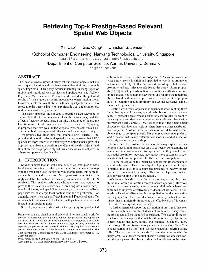
To illustrate the effect of supporting prestige-based object rele-vance, consider the query “shoes” at location P in Figure 1. Circlesrepresent shops selling shoes or jeans, with centers representinglocations and areas representing relevance to the query. Existingspatial keyword search techniques (e.g., [8]) rank R5 as the top-1result since R5 is relevant and closest to P. However, R4 is moreattractive because it has more nearby shops that are relevant to thequery and also is close to the query location.

Figure 1: Prestige propagation exampleIn our proposal for prestige-based relevance (denoted as PR) of

objects to queries, the PR score of an object is affected by the PRscores of its neighbors. This motivates us to employ a PageRank-like random walk mechanism for the propagation of prestige.

Conceptually, given the example query above, the PR scores ofthe objects are computed as follows: We build a graph with theobjects as the nodes. Two nodes are connected by an edge if theobjects are close and their text descriptions are similar. Myriadsof random surfers are initially placed at the nodes that contain thequery term “shoes” (i.e., R4, R5, R6, R7). The number of randomsurfers at a node is proportional to the textual relevance between thenode and the query, which is the initial prestige-based relevance ofthe node. At each step, each random surfer either moves to an ad-jacent node following a link in the graph with a certain walkingprobability (depending on the distance between the nodes), or itrandomly jumps to the initial set of nodes containing “shoes” with-out following any link, again with a certain probability (dependingon the well-known damping factor [5]). The expected percentageof surfers at each node eventually converges, and the convergedpercentage of surfers at a node represents the PR score of the node.

The concept of PR is inspired by the concept of personalizedPageRank [16], where a subset of web pages share the initial pres-tige uniformly (rather than all web pages as in PageRank), and itsapplications to keyword search in Entity-Relation graphs [1, 6].

The above random walk process has unique features that ren-der a direct application of PageRank [5] inadequate. PageRank isused to compute the objects’ global importance, which is query-independent, and it has no preferences for any particular nodes. Ourproblem is very different: each query has a set of preference objectsbased on the initial relevance scores, and thus random surfers startfrom this set of objects and jump to them. For example, given a“jeans” query at point P, R1 is the best result rather than R4, whichis best if the query is for “shoes.”

We propose a new type of query, called the Location-aware top-kPrestige-based Text retrieval (LkPT) query, that takes into accountboth location proximity and prestige-based text relevance (PR). Thequery retrieves a list of k objects ranked according to their spatialdistances and PR scores with respect to the query.

The LkPT query is expensive to compute, especially due to thePR scores. A straightforward approach to computing the LkPTquery is to adapt the algorithms for computing Personalized PageR-ank Vectors (PPVs) [1, 4, 6, 12, 16] to computing the PR scores ofall objects in the spatial object graph, to use an R-tree for comput-

ing spatial distances, and then to combine the two scores. How-ever, this solution is expensive. First, it is expensive to computePR scores for a large graph at query time using existing algorithmsfor PPVs. Second, it is impractical to pre-compute PPVs for eachnode in terms of either pre-computation time or the storage require-ments [16]—|V |2 space is needed to store the PPVs for all objects.Third, it is a waste to compute the spatial distance and PR scores ofall objects and then rank them to find the top-k results.

We note that the spatial object graph has unique properties thatrender it different from the web link graph [16] and the entity-relation graph [1, 6].

• Similar spatial objects often co-locate geographically. Forexample, shops often co-locate, as do, e.g., bars. Therefore,spatial objects tend to naturally form subgraphs.

• The number of nodes in a subgraph is constrained by geog-raphy. Thus, subgraphs will be of relatively modest size.

Properties like these enable us to develop approaches that speedup PR scoring. We propose two novel algorithms for the efficientcomputation of the LkPT query.

ES-EBC (Early stop extended bookmark coloring): We provethat if the distance between a node and the query point exceeds acertain threshold, the node will not affect the PR scoring of the top-k objects. Therefore, we need only consider nearby nodes whenpropagating PR, which speeds up the PR scoring substantially. Wealso show how to estimate lower and upper bounds on the PR scoreof each object in each iteration during scoring. Utilizing thesebounds, we derive conditions for when further iterations will notchange the ranking order of the top-k objects and we stop iterating.

S-EBC (Subgraph-based extended bookmark coloring): Wepropose an approximate solution to PR scoring with performanceguarantees. We organize spatial objects and their text descriptionsusing the external memory IR-tree [8]. Hence, the spatial objectsare grouped into subgraphs based on their locations, with each sub-graph corresponding to a leaf node of the IR-tree. We prove thatthe PR scores of the nodes in a subgraph can be computed by PRpropagation within the subgraph and contributions from the borderobjects that connect the subgraph with other subgraphs. This en-ables PR scoring w.r.t. subgraphs rather than on the whole graph.Next, we propose a novel approach to estimating an upper boundon the PR scores of the objects in each subgraph. This bound to-gether with the distance of a subgraph to the query is used to choosewhich subgraphs to process and in which order.

Empirical studies with real data offer insight into the effective-ness of LkPT queries and the efficiency of the proposed algorithms.

The rest of the paper is organized as follows. Section 2 definesthe LkPT query. Section 3 details the proposed algorithms. In Sec-tion 4, we report on the empirical studies. Section 5 concludes, andan appendix offers a variety of additional detail.

2. PROBLEM DEFINITIONLet D be a set of spatial objects. Each object o in D has a text

description o.ψ and a location o.µ. Similarly, a Location-awaretop-k Prestige-based Text retrieval (LkPT) query Q = 〈ψ, µ〉 has alocation Q.µ and a set of keywords Q.ψ.

Let Dist(Q, o) denote the Euclidean distance between the loca-tions of query Q and object o, and let Sim(Q, o) denote the rel-evance between the keyword component of query Q and the textdescription of object o. We use the Vector Space Model [23], oneof the most popular ranking functions, for computing Sim(Q, o),while using the TF-IDF weighting scheme to represent the text de-scriptions of objects (details are in Appendix A).

374

To compute the PR scores of objects, we define a weighted, undi-rected graph G = (V, E) overD, where each node in V correspondsto a spatial object and edge set E includes an edge 〈oi, oj〉 iff thefollowing two conditions are satisfied: 1) Dist(oi, oj) ≤ λ and 2)Sim(oi, oj) ≥ ξ, where λ and ξ are threshold parameters. Theweight of edge 〈oi, oj〉 in E is Dist(oi, oj).Prestige-Based Relevance (PR). The final PR vector ~p fulfills thefollowing equation:

~p = (1− α)CT~p + α ~uQ,

~uQ = [v1, ..., v|D|]T , vi = Sim(Q, oi), 1 ≤ i ≤ |D|, (1)

where C is the normalized adjacency matrix of graph G such that∑j∈V C(b, j)= 1, where C(b, j) represents the normalized weight

from node b to node j; and column vector ~uQ is the initial PR vec-tor in which each element is the relevance of an object.

Parameter α represents the probability of a random surfer jump-ing to the set of initially relevant spatial objects (vi > 0) instead offollowing the edges in the graph. Interestingly, parameter α can beused to balance the relevance of an object and the effect of its rel-evant neighbors, i.e., the parameter allows for tuning according touser-specific requirements. In particular, smaller values of α favorobjects with nearby relevant objects, while larger values of α favorobjects with high initial PR scores.

To understand the random walk process for each object b, its PRscore ~p(b) can be rewritten as follows:

~p(b) = α ~uQ(b) + (1− α)∑j∈V

C(j, b)~p(j), (2)

where ~uQ(b) is the initial PR score of b.The iterative computation diffuses the PR score of each object

across the graph. In the beginning, each object gets its initial PRscore according to its text relevance to the query. At each step, an αfraction of the PR score is held by each node, while the remaining(1−α) flows by following the links of the graph. This propagationcontinues until all the prestige is distributed cross the graph. Thefinal PR scores take into account both the original relevance scoresand the effect of neighbor nodes.

The PR vector is inspired by the of personalized PageRank vec-tor (PPV) [16] of preference vector ~uQ. In the original PPV [16],a set of preferred objects in the preference vector are assigned uni-form initial scores, while we assign an initial score to an object thatis in proportion to its text relevance to the query.LkPT Query Definition. Intuitively, an LkPT query retrieves k ob-jects from database D ranked according to a combination of theirdistances to the query location and their PR scores for the query.Formally, given a query Q = (ψ, µ), where Q.ψ is a locationdescriptor and Q.µ is a set of keywords, the objects returned areranked according to a ranking function f(Dist(Q, o), Pr(Q, o)),where Dist(Q, o) is the Euclidian distance between Q and o andPr(Q, o) is the PR score of o with respect to Q. An LkPT querybecomes an LkT query [8] in the extreme case of α = 1 (Equa-tion 2), i.e., we disregard the effects of nearby relevant objects.Problem Statement. We address the problem of efficiently an-swering LkPT queries.

The paper’s proposals are applicable to a wide range of rank-ing functions that are monotone with respect to the distance prox-imity Dist(Q, o) and the PR score Pr(Q, o). We follow existingwork [8,20] and use a linear combination of the normalized factorsfor ranking an object o with respect to a query Q:

RS(Q, o) = (1− β)(1− Pr(Q, o)) + βDist(Q, o)

maxD(3)

where β ∈ (0, 1) is used to balance the PR score and the loca-tion proximity; Euclidian distance Dist(Q, o) between query Q

and object o is normalized to a value between 0 and 1 by a con-stant maxD, which can be the maximum distance between twoobjects in D or the maximum distance that can be accepted by theusers; and Pr(Q, o) is the PR score of object o w.r.t. query Q andusually takes a value between 0 and 1. This function computes theranking score of each object given an LkPT query.

Note that parameter β allows to set the preference between thePR score and the location proximity at query time.

3. PROPOSED SOLUTIONS3.1 Baseline Algorithm

As a baseline, we present an improvement of the straightforwardsolution mentioned in the introduction.

In the straightforward solution, we compute PR scores for allobjects and the distances between all objects and the query, uponwhich we rank the objects based on the combined scores. We focuson computing the costly PR scores.

We choose to adapt the bookmark-coloring algorithm (BCA) [4],an elegant algorithm for computing PPVs, to computing the PRscores. We first extend the in-memory BCA algorithm to work insecondary memory. We read the graph in large blocks that eachexploit the memory available, and do the iterative propagation ina per-block manner. The computation stops when the termina-tion condition for the graph is met. A block is likely to be readand written multiple times since it may receive PR scores fromother blocks that need to be distributed. Second, we BCA, whichworks on unweighed graph for a single preferred object, to sup-port PR score computation for a general preference vector ~uQ on aweighted graph.

Algorithm 1 details the resulting Extended BCA (EBC) algo-rithm. Let ~p denote the PR score that each object already has, let~q denote the PR score that each object needs to distribute, and letoutPR be the vector of the sum of the PR scores that need to bedistributed in each graph block.

Algorithm 1 EBC(Q)Input: query QOutput: The PR score of each object1: compute the text relevance of each object to Q and compute ~uQ

2: ~q ← ~uQ, ~p ← ~0, outPR ← ~03: blockQueue← NewPriorityQueue()4: for each object b do outPR(b.block) ← outPR(b.block) + ~q(b)5: for each block bg do blockQueue.Enqueue(bg)6: while ‖~q‖1 ≥ ε do7: bgi = blockQueue.Dequeue()8: read the graph block bgi

9: outPR(bgi) ← 010: Queue ← NewQueue()11: for each object n s.t. n ∈ bgi and ~q(n) > 0 do12: Queue.Enqueue(n)13: while not Queue.Empty() do14: b ← Queue.Dequeue()15: if ~q(b) > ε then16: ~p(b) ← ~p(b) + α~q(b)17: for each out-neighbor j of b do18: if ~q(j) = 0 and j ∈ bgi then Queue.Enqueue(j)19: outV ← (1− α)C(b, j)~q(b)20: ~q(j) ← ~q(j) + outV21: if j /∈ bgi then22: outPR(j.block) ← outPR(j.block) + outV23: ~q(b) ← 024: blockQueue.Update()25: return ~p

We compute the text relevance of each object to the query Qusing an inverted list index and then construct the preference vec-

375

tor ~uQ according to Equation 1 (line 1). We use a priority queueblockQueue whose key is the accumulated outgoing PR score thatneeds to be propagated in each block (lines 4–5). In each graphblock, we modify the propagation mechanism of BCA to accom-modate edge weights and multiple objects in the preference vector.

We use a queue Queue to store the objects that have PR scoresthat need to be distributed (lines 10–12). Specifically, for the PR~q(b) that needs to be distributed at an object b, we assign α~q(b) tob (line 16) and (1 − α)~q(b) to its neighbors according to the edgeweights (lines 17–20). We update the PR score that needs to bedistributed for each block (lines 21–22).

When the PR score of each object that needs to be distributed issmaller than the propagation threshold ε, we stop the propagationwithin a block (line 15). When the PR score to be distributed issmaller than the tolerance threshold ε (line 6), we stop the propa-gation over the graph and return PR vector ~p, each element of whichrepresents the PR score Pr(Q, o) of object o. We thus use ε and εas the termination conditions, as in BCA [4] and its variant [13].

This method is inefficient because it computes PR scores and dis-tances for all objects. The PR scores of objects are inter-dependentand need to be computed together, while the distance scores canbe computed individually. Thus, inspired by the Threshold algo-rithm [11], we develop two improved baseline algorithms that avoidunnecessary distance score computations. These two algorithmsare covered in Appendix B.1.

3.2 Early Stop EBC Algorithm (ES-EBC)PR scores are much more costly to compute than distances be-

cause they require iterations over possibly large graphs. We thusproceed to propose two new techniques for speeding up the com-putation of PR scores. First, we show how to stop the iterativePR score computation early, using a new stopping condition (The-orem 1). Second, we show how to disregard objects further awayfrom the query than a certain distance (Theorem 2). All proofs arefound in Appendix C.

As before, let ~p denote the vector of the PR score that each objectalready has, and let ~q denote the vector of the outgoing PR scorethat each object needs to distribute.

LEMMA 1. Let ~pi(b) denote the PR score of object b in the i-thiteration during PR scoring. Then ~pi(b) ≤ ~pi+1(b).

LEMMA 2. Given an object b, the final PR value ~p(b) of b andthe value ~pi(b) of b in the i-th iteration fulfill the following:

~pi(b) ≤ ~p(b) ≤ ~pi(b) + α2max(~qi) + (1− α)‖~qi‖1,where max(~qi) is the maximum element in ~qi in the i-th iteration,and ‖ · ‖1 is the 1-norm.

Lemma 2 follows previous work [13]. The current ranking scoreCRS(b) of an object b is computed according to Equation 3 at thecurrent (i-th) iteration of PR scoring. We estimate lower and upperbounds on the ranking score for each object in the i-th iteration asfollows:

Upper(b) = CRS(b)

Lower(b) = CRS(b)− (1−β)(α2max(~qi) + (1−α)‖~qi‖1)(4)

The upper bound holds because the distance between an object andthe query is constant, while its PR score increases in each iteration(Lemma 1). We obtain the lower bound based on Lemma 2 andEquation 3.

THEOREM 1. Let priority queue Lr record the current top-(k+1) objects seen, the key being the objects’ PR scores. It is guar-anteed that the top-k objects have been found if the k-th and the

(k + 1)-st objects, represented by Lr(k) and Lr(k + 1), respec-tively, satisfy the following condition:

Upper(Lr(k)) < Lower(Lr(k + 1))

The PR score computation stops iterating when the conditionin Theorem 1 is satisfied, i.e., the current top-k objects all havesmaller final ranking scores than those of all other nodes.

THEOREM 2. Given a query Q, a set of candidate objects C,and a spatial cell Ωi, objects contained in Ωi can be disregardedduring propagation if the following is satisfied:

minDist(Q, Ωi) > λ log1−α

ε

outC(Ωi)+ Dist(Q, os),

where minDist(Q, Ωi) is the minimum distance between Q and Ωi,λ is the distance threshold used when building the object graph; αand ε are as explained in Algorithm 1; os is the object in C furthestaway from query Q; and outC(Ωi) stores the aggregated PR scorethat needs to be distributed in Ωi.

The condition stated in Theorem 2 guarantees that the objects incell Ωi will neither become top-k results nor affect the PR scoresof the top-k results. Thus, the objects in the cell can be disregardedduring the propagation of scores.

The algorithm that exploits the early stopping conditions first di-vides the graph into blocks according to the locations of the spatialobjects such that each block fits into memory. Each block is fur-ther divided into a grid of spatial cells. Then nearest neighbors areretrieved incrementally [14] using the R*-tree [3]. For each near-est neighbor object o, the block graph containing o is read cell bycell: for each cell the algorithm checks whether it can be prunedaccording to Theorem 2; if it cannot, it reads the part of the graphcorresponding to the cell. Then it iterates in the block to get thelocal PR scores for the objects in the block.

The algorithm keeps track of the current top-(k + 1) objects.When the ranking score of the k-th object is smaller than the lowerbound (the minimum possible) ranking score of the current nearest-neighbor object o, i.e., ∆ = β Dist(Q,Lr(k))

maxD), the nearest-neighbor

retrieval stops because no unseen object has a lower ranking scorethan has object o (since unseen objects no closer to the query thano) and thus cannot be a top-k object.

This way, we obtain a set of candidate top-k objects. However,these do not necessary constitute the final result since PR scoreswere only propagated inside a block. We need to propagate the PRscores across blocks while still using Theorems 1 and 2. Additionalexplanations and pseudo-code are available in Appendix B.2.

3.3 Subgraph-Based EBC Algorithm (S-EBC)

3.3.1 Overview of the AlgorithmRecall that the baseline and ES-EBC algorithms need to propa-

gate PR scores on the whole graph. To compute PR scores withinsome selected subgraphs, we develop several techniques.

First, we show that PR scores can be computed by the combi-nation of two parts: the PR score propagation within a subgraphand the PR contributed by the propagations from other subgraphs,which can be computed from pre-computed distribution vectors ofthe border nodes that connect the subgraph with other subgraphs(see Section 3.3.2). This enables us to compute PR scores withrespect to a subgraph.

Second, we propose an approach to identifying the subgraphsthat need to be checked to find the top-k results, thus avoidingchecking all subgraphs. This is enabled by a novel approach toestimating upper bound PR scores of objects in a subgraph, given aquery.

376

Specifically, we organize the spatial objects by extending the ex-ternal memory IR-tree [8]. The spatial objects are grouped intosubgraphs so that each subgraph corresponds to a leaf node of theIR-tree. We enrich the nodes of the tree with pre-computed infor-mation (see Section 3.3.3) and show that by utilizing this informa-tion, we can compute an upper bound PR score at each node for aquery.

The upper bound PR scores together with the distance of a sub-graph to the query are used to choose which subgraphs to processat query time. If the best estimated ranking score of nodes in a sub-graph exceeds (the smaller a score, the better) the score of the k-thobject, the subgraph cannot contribute to the top-k results and canbe pruned.

Based on this, we propose an approximate algorithm with perfor-mance guarantees for answering LkPT queries (see Section 3.3.4).The approximation occurs because we do not process all subgraphs.

3.3.2 Subgraph-Based PR ScoringWe present a decomposition method that enables us to compute

PR scores with regard to subgraphs.Assume that we have already partitioned the graph G into m sub-

graphs G1, ..., Gm (to be discussed in Section 3.3.3). Let border(Gi)be the set of border objects of Gi that connect Gi with other sub-graphs. Also, let H be the set of the border objects of all subgraphs,i.e., H =

⋃i∈[1,m] border(Gi).

For each border object b, we pre-compute and store a vector ~GPb

that describes how to distribute the unit initial PR score from b overthe whole graph. Note that the number of border objects is muchsmaller than the number of objects in the database. In a vector ~Prb,most of the elements are 0 since in spatial graphs, a node b usuallyonly affects the objects in nearby subgraphs. We do not need tostore the value 0.

We proceed to show that the PR score vector of an object, whichis assigned the unit initial PR score, can be computed by propaga-tion within its subgraph together with the propagations contributedby the border nodes, which we capture in pre-computed PR scorevectors of border nodes. We denote the PR scores computed withina subgraph as the local PR scores ( ~LP), and we denote the PRscores on the whole graph as the (global) PR scores ( ~Pr). We havethe following lemma and theorem:

LEMMA 3. Given a node b and a subgraph Gi containing ob-ject b, we can compute the PR score vector of b as follows:

~Prb = ~LPrb +∑

h∈border(Gi)

~APb(h) · ~Prh,

where ~APb(h) is the accumulated PR score of border node h dur-ing the local propagation within subgraph Gi.

THEOREM 3. Given a query Q, its PR score vector is computedas:

~PrQ =

m∑j=1

∑o∈Gj

Sim(Q, o)( ~LPro +∑

h∈border(Gj)

~APo(h) · ~Prh)

Sim(Q, o) is the similarity of query Q and the description of objecto according to the vector space model (Appendix A).

Theorem 3 allows us to decompose the computation of PR scor-ing. Given a query Q and a subgraph, we compute the text rel-evance to Q of each object in the subgraph. We distribute thesescores following the links within the subgraph: when we reach aborder node, the node accumulates the value distributed to it; ifwe meet a non-border node in the subgraph, we increase its PR

score by a portion of the scores and distribute the rest to its out-neighbors, as in Algorithm 1. Having processed all subgraphs (i.e.,we distribute PR scores within each subgraph), we use the globalPR vector of each border object in a subgraph to update the PRscores for all the objects according to Theorem 3.

3.3.3 Indexing and Ranking Score EstimationTo efficiently process an LkPT query, we need to organize the

spatial objects into subgraphs. We proceed to briefly introduce theindex structure used for organizing objects and then focus on howto estimate an upper bound PR score for each node for a single-termas well as a multi-term query.Index structure—IR-tree. We extend the IR-tree [8] index struc-ture to organize spatial objects and capture the pre-computed in-formation needed for upper bound estimation. It is also used topartition the graph.

A leaf node L in the IR-tree contains a number of entries of theform 〈o, o.µ〉, where o is the identifier of an object and o.µ is thebounding rectangle of the object. A leaf node corresponds to asubgraph and contains a pointer to the subgraph at the node and theglobal PR score vector of the border objects of the subgraph.

A non-leaf node R contains a number of entries of the form〈cp, Ω〉, where cp points to a child node and Ω is the minimumbounding rectangle of all rectangles of entries in the child node.

Each node contains a pointer to an inverted file that describes theobjects in the subtree rooted at the node. The inverted file for anode X contains: 1) A vocabulary of all distinct terms in the textdescriptions of the objects in the subtree rooted at X . 2) A set ofposting lists, each of which relates to a term t. Each posting list is asequence of pairs 〈cp, wtcp,t〉, where cp is a child of X and wtcp,t

is the upper bound PR score of objects in the subtree rooted at cpfor term t.

It is challenging to develop an effective approach to estimatingthe upper bound PR score of a node even for a single-keywordquery (i.e., wtcp,t), much less a multi-keyword query. It is com-putationally prohibitive to pre-compute the exact PPVs for eachobject [16], and this also holds for PR score vectors since they needsimilar computation. Note that the purpose of pre-computing andstoring the upper bounds is that we can then utilize them to prunethe search space at query time for an LkPT query (this will becomeclear shortly).Upper bound PR score for single-keyword queries. We first con-sider a leaf node; it is straightforward to derive an upper bound fora non-leaf node from those of its child nodes. We estimate the up-per bound for a leaf node by the sum of the upper bound PR scoresfrom the propagation within the node and the maximum contribu-tion from other subgraphs. Let L be a leaf node that correspondsto a subgraph Gi. Let maxGPr(t, L) denote the estimated upperbound PR score of the objects in L for (query) term t. To estimatemaxGPr(t, L), we need the initial PR score of a subgraph Gi for aquery term t, denoted as IPS(t,Gi).

DEFINITION 1. The initial PR score of Gi for t is computed asfollows:

IPS(t,Gi) =∑o∈Gi

Sim(t, o)

Here, Sim(t, o) is the similarity between term t and the descriptionof object o according to the Vector Space Model (Appendix A).

We first present a lemma on how to estimate a maximum localPR score within a subgraph Gi given a query term t. This is the PRscore without considering the effects of other subgraphs.

LEMMA 4. The maximum local PR score maxLPr(t,Gi) canbe estimated as:

377

maxLPr(t,Gi) =1 + α− α2

2− αmaxo∈Gi

(Sim(t, o))

+1− α

2− αIPS(t,Gi)

Here, maxo∈Gi(Sim(t, o)) is the largest initial PR score in sub-graph Gi for term t.

Based on this lemma, we get the following theorem.

THEOREM 4. We estimate maxGPr(t,Gi), the global upperbound PR score of an object in Gi for t, as follows:

maxGPr(t,Gi) = maxLPr(t,Gi)+∑

j 6=i

IPS(t,Gj) · maxbn∈border(Gj),b∈Gi

( ~Prbn(b))

IPS(t,Gi) is computed according to Definition 1, and IPS(t,Gj)·maxbn∈border(Gj),b∈Gi

( ~Prbn(b)) represents the maximum possi-ble PR score that can be propagated from Gj to a node in Gi.

We can now explain the weight wtcp,t in the inverted file. Ata leaf node X , the upper bound of each object cp is computed asSim(cp.ψ, t) (defined in Appendix A); At the parent node X of aleaf node, wtcp,t = maxGPr(t, Gcp) (computed according to The-orem 4). For other nodes, wtcp,t is the largest PR score among thechild nodes of cp, i.e., maxR∈cp.children() wtt,R.Upper bound PR score for multi-keyword queries. Based on thepre-computed upper bound PR score for a single keyword query,we propose an approach to estimating the upper bound PR scorefor a multi-keyword query.

LEMMA 5. Given a subgraph Gi, we compute its initial PRscore (IPS) for a query Q as follows:

IPS(Q,Gi) =∑

t∈Q.ψ⋂Gi.ψ

wQ.ψ,t

WQ.ψIPS(t,Gi),

where wQ.ψ,t and WQ.ψ are defined in Appendix A and IPS(t,Gi)is computed according to Definition 1.

Lemma 5 provides a way of computing the initial PR scores of aquery Q in a subgraph Gi. We proceed to present how to estimatethe upper bound PR score of each node in the IR-tree for a queryQ.

DEFINITION 2. Given a query Q and a node X in an IR-tree,the largest possible PR score of objects in X , maxPr(Q, X), isdefined as:

maxPr(Q, X) =∑

t∈Q.ψ⋂

X.ψ

wQ.ψ,t

WQ.ψmaxGPr(t, X),

where wQ.ψ,t and WQ.ψ are defined in Appendix A.THEOREM 5. Given a query Q and a leaf node X that encloses

a set of objects XO = o1, . . . , om, the following holds:∀o ∈ XO; (maxPr(Q, X) ≥ Pr(Q, o))

We proceed to present the minimum spatial-PR score distance,minRS, which is needed for the query processing. Given a queryQ and a node X in the IR-tree, the metric minRS offers a lowerbound on the actual spatial-PR score distance between query Qand the objects in node X . This bound can be used to order andefficiently prune the search space in the index.

DEFINITION 3. Given a query Q and a node X , the minimumspatial-PR distance, denoted by minRS(Q, X), is defined as:

minRS(Q, X) = (1−β)(1−maxPr(Q, X))+βDist(Q.µ, X.Ω)

maxD

Here, maxPr(Q, X) is the upper bound PR score of objects in Xfor query Q (cf. Definition 2).

THEOREM 6. Given a query Q and a node X whose rectangleencloses a set of objects XO = o1, . . . , om, the following is true:

∀o ∈ XO; (minRS(Q, X) ≤ RS(Q, o))

The extended IR-tree used in this paper and the original IR-tree [8] share a similar data structure. However, the inverted filesin the two indexes store different contents. The novelty of the ex-tended IR-tree is its approach to estimating upper bound PR scores.

3.3.4 Subgraph-Based EBC Algorithm (S-EBC)We proceed to describe the S-EBC algorithm that exploits the

techniques just presented.The main idea is to choose subgraphs that are more likely to con-

tain top-k results for a query Q and then compute the PR scores inthe selected subgraphs. For a node X in the IR-tree, we estimate itslargest possible PR score according to Definition 2, and we com-pute its distance to the query. Thus, we can compute the smallestpossible ranking score (minRS(X, Q) in Definition 3; the smallerthe score, the better).

We use a priority queue queue to keep track of the nodes thathave yet to be visited; the smallest possible ranking score is usedas the key. When the head of the queue is a leaf node, i.e., itscorresponding subgraph Gi has the lowest possible ranking score,we process the subgraph using the approach from Section 3.3.2.When the propagation within the subgraph completes, we have alocal PR score for each object in Gi, and we use the PR scores heldby the subgraph’s border objects to update the global PR scores ofall the objects (for object o, according to Theorem 3).

We proceed to process the next subgraph using the priority queue.The processing continues until the smallest possible ranking scoreof the unvisited head node of the priority queue exceeds the rankingscore of the current k-th result; we can then stop since no unvisitedobject can become a top-k result.

It is guaranteed that the unprocessed subgraphs (leaf nodes) donot contain top-k objects. However, they may affect the PR scoresof the current top-k objects. To ensure this effect is within a cer-tain bound, some postprocessing is needed. When building an IR-tree, we append the following pre-computed information to eachleaf node (subgraph Gi) of the IR-tree: a set of the IDs of the sub-graphs that affect Gi, denoted by Gi.Near and a factor describingthe maximum possible effect of a subgraph on an object in Gi (e.g.,for a subgraph Gj , the factor is maxbn∈border(Gj),b∈Gi

( ~Prbn(b)),according to Theorem 4).

In the postprocessing, we find the set SS of subgraphs con-taining the current top-k objects. For each subgraph Gi in SS,we then find Gi.Near, the set of subgraphs that affect the PRscores of objects in Gi. For each subgraph Gj in Gi.Near, if itis not yet processed, we compute its maximum possible effect onan object in Gi, denoted by maxEF(Gj ,Gi), according to Theo-rem 7. We sort the subgraphs in Gi.Near in ascending order ofmaxEF(Gj ,Gi), and we then find the m-th subgraph for whichSumErr =

∑j=[1,m−1] maxEF(Gj ,Gi) < σ and SumErr +

maxEF(Gm,Gi) ≥ σ.Then starting from the m-th subgraph, for each subgraph in the

sorted Gi.Near, we do local propagation and update the PR scoresof objects. We then update the list of the current top-k objects.If new objects are in the top-k and their corresponding subgraphsare not in SS, we include these subgraphs in SS and repeat theabove steps until we have processed all subgraphs in SS. The post-processing ensures that the maximal possible error in the rankingscore of each top-k object is smaller than the error bound σ.

378

THEOREM 7. Given a query Q, the maximum possible PR scorethat subgraph Gj can propagate to an object in Gi is:

maxEF(Gj ,Gi) = IPS(Q,Gj) maxbn∈border(Gj),b∈Gi

( ~Prbn(b))

Pseudo-code and further explanations are given in Appendix B.3.

4. EXPERIMENTAL STUDY4.1 Experimental SettingsAlgorithms. In addition to the two proposed algorithms, ES-EBCand S-EBC, we compare with the two baseline approaches in Ap-pendix B.1. As Baseline 1 outperforms Baseline 2 significantly, weonly report results for Baseline 1 and refer to this as “Baseline.”Data and queries. We use three datasets that are real or based onreal datasets. Table 1 shows some properties ff the datasets; addi-tional descriptions are provided in Appendix D. Hotel is a smalldataset while GN is much bigger. The objects in both datasets haveshort descriptions. Web is a medium-sized dataset whose objectshave long descriptions. We evaluate our approaches on these threedifferent datasets.

Property Hotel Web GNTotal number of objects 20,790 579,727 1,868,821

Total number of unique words 602 2,899,175 222,409Total number of words 80,845 249,132,883 18,374,228

Table 1: Dataset properties

We generate 4 query sets, in which the number of keywords is1, 2, 3, and 4, respectively, in the space of GN, and we generate4 similar query sets for the space of Spam and Hotel. Each setcomprises 200 queries, and each query is randomly generated. Wereport average costs of the queries in each query set.Setup. The IR-tree index structure is disk resident, and the pagesize is 16KB. The number of children of a node in the IR-tree iscomputed given the fact that each node occupies a page. This trans-lates to 400 children per node in our implementation. The defaultvalues for parameters are as follows: k is 10, the number of querykeywords is 2, α is 0.5 (Equation 2), and β is 0.5 (Equation 3) forall algorithms. S-EBC needs an extra parameter σ (to control itserror bound; Section 3.3.4) that is set to 0.0001. Two threshold pa-rameters for building graphs λ and ξ (Section 2) are set at 2 km and0.5, respectively.

All algorithms were implemented in VC++, and run on an In-tel(R) Core(TM)2 Duo CPU T7500 @2.66GHz with 2GB RAM.

4.2 Experimental ResultsThe reported results are on GN if not stated otherwise.

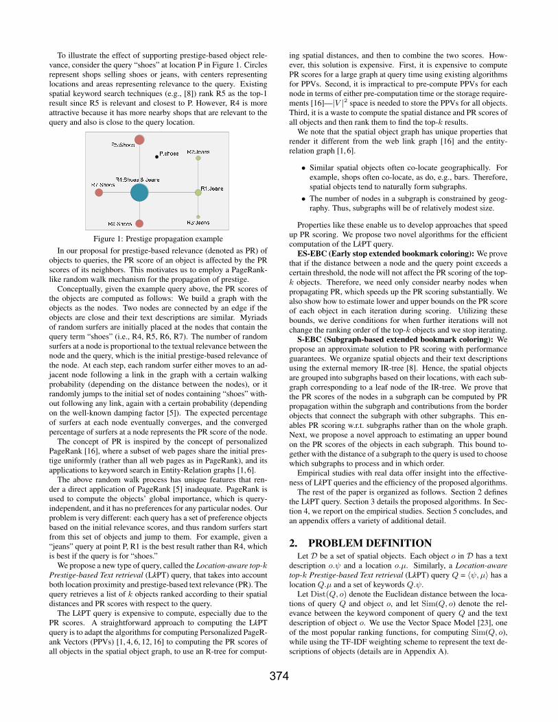
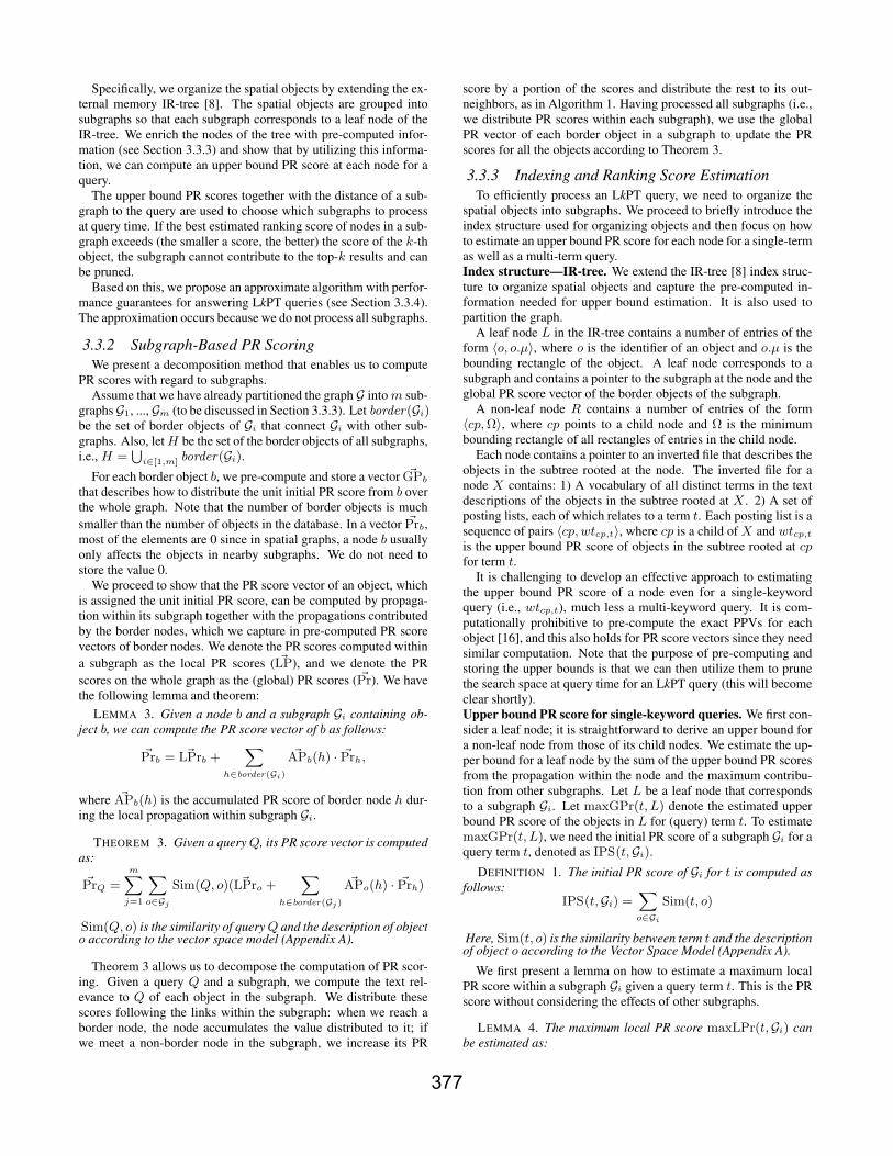
Varying k in LkPT. Figure 2 show the results of varying k whenusing the default settings for the other parameters.. Note that they-axis uses a logarithmic scale.

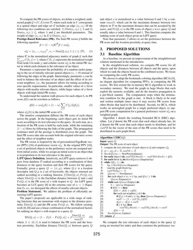
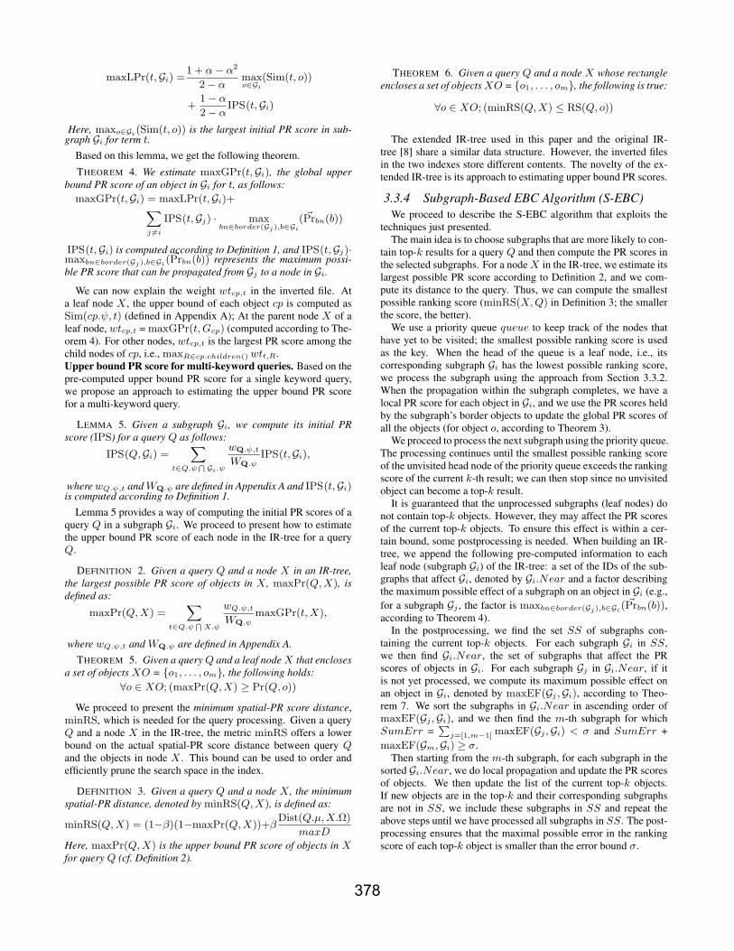
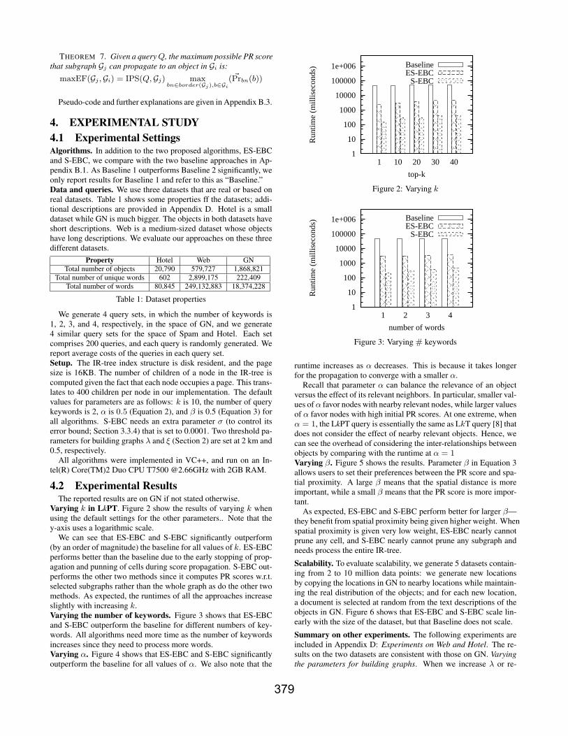
We can see that ES-EBC and S-EBC significantly outperform(by an order of magnitude) the baseline for all values of k. ES-EBCperforms better than the baseline due to the early stopping of prop-agation and punning of cells during score propagation. S-EBC out-performs the other two methods since it computes PR scores w.r.t.selected subgraphs rather than the whole graph as do the other twomethods. As expected, the runtimes of all the approaches increaseslightly with increasing k.Varying the number of keywords. Figure 3 shows that ES-EBCand S-EBC outperform the baseline for different numbers of key-words. All algorithms need more time as the number of keywordsincreases since they need to process more words.Varying α. Figure 4 shows that ES-EBC and S-EBC significantlyoutperform the baseline for all values of α. We also note that the

1

10

100

1000

10000

100000

1e+006

1 10 20 30 40

Run

time

(mill

isec

onds

)

top-k

BaselineES-EBC

S-EBC

Figure 2: Varying k

1

10

100

1000

10000

100000

1e+006

1 2 3 4R

untim

e (m

illis

econ

ds)

number of words

BaselineES-EBC

S-EBC

Figure 3: Varying # keywords

runtime increases as α decreases. This is because it takes longerfor the propagation to converge with a smaller α.

Recall that parameter α can balance the relevance of an objectversus the effect of its relevant neighbors. In particular, smaller val-ues of α favor nodes with nearby relevant nodes, while larger valuesof α favor nodes with high initial PR scores. At one extreme, whenα = 1, the LkPT query is essentially the same as LkT query [8] thatdoes not consider the effect of nearby relevant objects. Hence, wecan see the overhead of considering the inter-relationships betweenobjects by comparing with the runtime at α = 1Varying β. Figure 5 shows the results. Parameter β in Equation 3allows users to set their preferences between the PR score and spa-tial proximity. A large β means that the spatial distance is moreimportant, while a small β means that the PR score is more impor-tant.

As expected, ES-EBC and S-EBC perform better for larger β—they benefit from spatial proximity being given higher weight. Whenspatial proximity is given very low weight, ES-EBC nearly cannotprune any cell, and S-EBC nearly cannot prune any subgraph andneeds process the entire IR-tree.

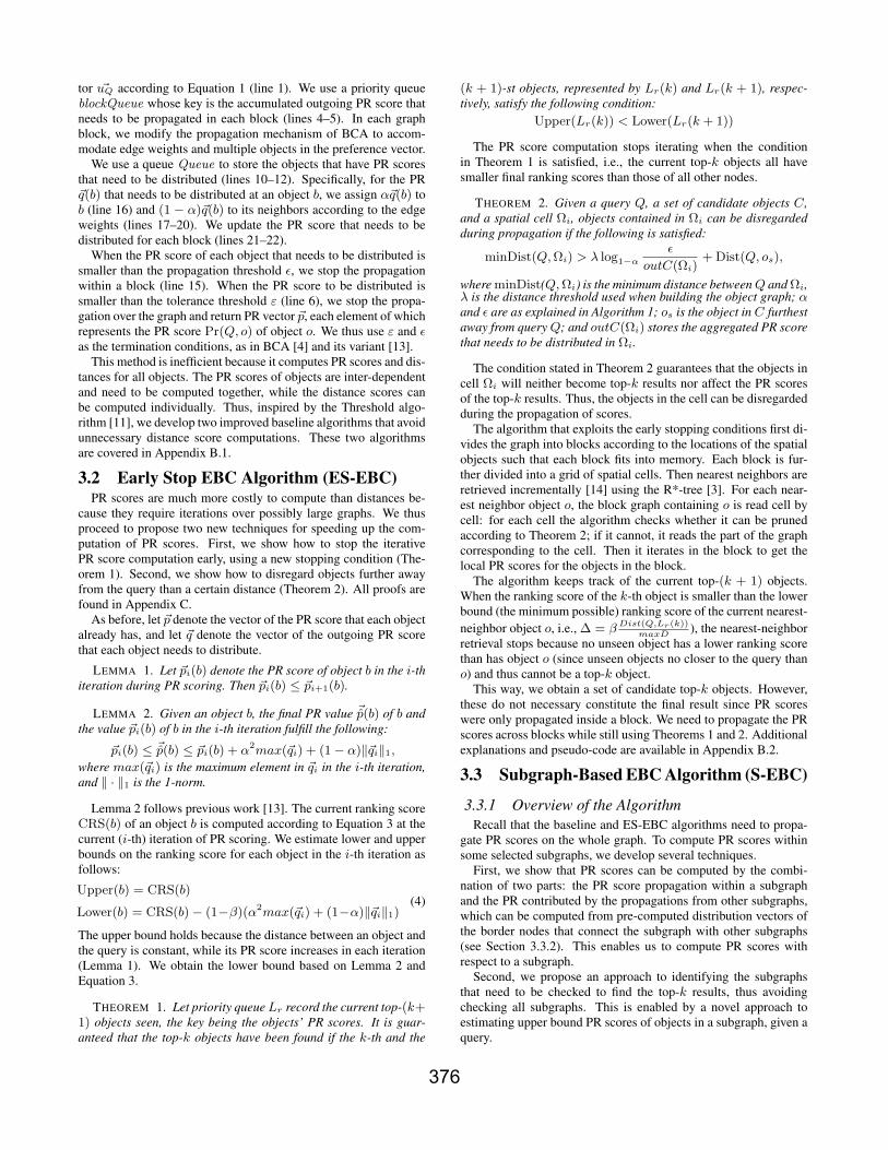
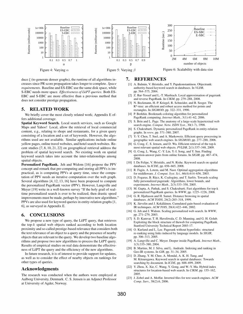
Scalability. To evaluate scalability, we generate 5 datasets contain-ing from 2 to 10 million data points: we generate new locationsby copying the locations in GN to nearby locations while maintain-ing the real distribution of the objects; and for each new location,a document is selected at random from the text descriptions of theobjects in GN. Figure 6 shows that ES-EBC and S-EBC scale lin-early with the size of the dataset, but that Baseline does not scale.

Summary on other experiments. The following experiments areincluded in Appendix D: Experiments on Web and Hotel. The re-sults on the two datasets are consistent with those on GN. Varyingthe parameters for building graphs. When we increase λ or re-

379

1

10

100

1000

10000

100000

1e+006

0.1 0.3 0.5 0.7 1

Run

time

(mill

isec

onds

)

α

BaselineES-EBC

S-EBC

Figure 4: Varying α

1

10

100

1000

10000

100000

1e+006

0.1 0.3 0.5 0.7 0.9

Run

time

(mill

isec

onds

)

β

BaselineES-EBC

S-EBC

Figure 5: Varying β

0

50

100

150

200

250

300

2M 4M 6M 8M 10M

Run

time

(sec

.)

number of objects

BaselineES-SBC

E-SBC

Figure 6: Scalability with data size

duce ξ (to generate denser graphs), the runtime of all algorithms in-creases since PR score propagation takes longer to complete. Spacerequirements. Baseline and ES-EBC use the same disk space, whileS-EBC needs more space. Effectiveness of LkPT queries. Both ES-EBC and S-EBC are more effective than a previous method thatdoes not consider prestige propagation.

5. RELATED WORKWe briefly cover the most closely related work; Appendix E of-

fers additional coverage.Spatial Keyword Search. Local search services, such as GoogleMaps and Yahoo! Local, allow the retrieval of local commercialcontent, e.g., relating to shops and restaurants, for a given queryconsisting of a location and a set of keywords. However, the algo-rithms used are not available. Similar applications include onlineyellow pages, online travel websites, and hotel search websites. Re-cent studies [7, 8, 10, 21, 22] on geographical retrieval address theproblem of spatial keyword search. No existing work on spatialkeyword search takes into account the inter-relationships amongspatial objects.Personalized PageRank. Jeh and Widom [16] propose the PPVconcept and remark that pre-computing and storing all PPVs is im-practical, as is computing PPVs at query time, since the compu-tation of PPV needs an iterative computation over the web graph.Several algorithms [4, 12, 13, 16] have been proposed to computethe personalized PageRank vector (PPV). However, Langville andMeyer [19] write in a well-known survey “If the holy grail of real-time personalized search is ever to be realized, then drastic speedimprovements must be made, perhaps by innovative new algorithms.”PPVs are also used for keyword queries in entity-relation graphs [1,6], as surveyed in Appendix E.

6. CONCLUSIONSWe propose a new type of query, the LkPT query, that retrieves

the top-k spatial web objects ranked according to both locationproximity and so-called prestige-based relevance that considers boththe text relevance of an object to a query and the presence of nearbyobjects that are relevant to the query. We develop two baseline algo-rithms and propose two new algorithms to process the LkPT query.Results of empirical studies on real data demonstrate the effective-ness of LkPT the query and the efficiency of the new algorithms.

In future research, it is of interest to provide support for updates,as well as to consider the effect of nearby objects on rankings forother types of queries.

AcknowledgmentsThe research was conducted when the authors were employed atAalborg University, Denmark. C. S. Jensen is an Adjunct Professorat University of Agder, Norway.

7. REFERENCES[1] A. Balmin, V. Hristidis, and Y. Papakonstantinou. Objectrank:

authority-based keyword search in databases. In VLDB,pp. 564–575, 2004.

[2] Z. Bar-Yossef and L.-T. Mashiach. Local approximation of pagerankand reverse PageRank. In CIKM, pp. 279–288, 2008.

[3] N. Beckmann, H.-P. Kriegel, R. Schneider, and B. Seeger. TheR*-tree: an efficient and robust access method for points andrectangles. In SIGMOD, pp. 322–331, 1990.

[4] P. Berkhin. Bookmark-coloring algorithm for personalizedPageRank computing. Internet Math., 3(1):41–62, 2006.

[5] S. Brin and L. Page. The anatomy of a large-scale hypertextual websearch engine. Comput. Netw. ISDN Syst., 30(1-7), 1998.

[6] S. Chakrabarti. Dynamic personalized PageRank in entity-relationgraphs. In www, pp. 571–580, 2007.

[7] Y.-Y. Chen, T. Suel, and A. Markowetz. Efficient query processing ingeographic web search engines. In SIGMOD, pp. 277–288, 2006.

[8] G. Cong, C. S. Jensen, and D. Wu. Efficient retrieval of the top-kmost relevant spatial web objects. PVLDB, 2(1):337–348, 2009.

[9] G. Cong, L. Wang, C.-Y. Lin, Y.-I. Song, and Y. Sun. Findingquestion-answer pairs from online forums. In SIGIR, pp. 467–474,2008.

[10] I. De Felipe, V. Hristidis, and N. Rishe. Keyword search on spatialdatabases. In ICDE, pp. 656–665, 2008.

[11] R. Fagin, A. Lotem, and M. Naor. Optimal aggregation algorithmsfor middleware. J. Comput. Syst. Sci., 66(4):614–656, 2003.

[12] D. Fogaras, B. Racz, K. Csalogany, and T. Sarlos. Towards scalingfully personalized pagerank: Algorithms, lower bounds, andexperiments. Internet Math., 2(3):333–358, 2005.

[13] M. Gupta, A. Pathak, and S. Chakrabarti. Fast algorithms for top-kpersonalized PageRank queries. In WWW, pp. 1225–1226, 2008.

[14] G. R. Hjaltason and H. Samet. Distance browsing in spatialdatabases. ACM TODS, 24(2):265–318, 1999.

[15] K. Jarvelin and J. Kekalainen. Cumulated gain-based evaluation ofIR techniques. ACM TOIS, 20(4):422–446, 2002.

[16] G. Jeh and J. Widom. Scaling personalized web search. In WWW,pp. 271–279, 2003.

[17] S. D. Kamvar, T. H. Haveliwala, C. D. Manning, and G. H. Golub.Exploiting the block structure of theweb for computing PageRank.Stanford University Technical Report 2003-17.

[18] O. Kurland and L. Lee. Pagerank without hyperlinks: structuralre-ranking using links induced by language models. In SIGIR,pp. 306–313, 2005.

[19] A. Langville and C. Meyer. Deeper inside PageRank. Internet Math.,1(3):335–380, 2004.

[20] B. Martins, M. J. Silva, and L. Andrade. Indexing and ranking inGeo-IR systems. In GIR, pp. 31–34, 2005.

[21] D. Zhang, Y. M. Chee, A. Mondal, A. K. H. Tung, andM. Kitsuregawa. Keyword search in spatial databases: Towardssearching by document. In ICDE, pp. 688–699, 2009.

[22] Y. Zhou, X. Xie, C. Wang, Y. Gong, and W.-Y. Ma. Hybrid indexstructures for location-based web search. In CIKM, pp. 155–162,2005.

[23] J. Zobel and A. Moffat. Inverted files for text search engines. ACMComp. Surv., 38(2):6, 2006.

380

APPENDIXA. VECTOR SPACE MODEL

The vector space model is defined as follows.

Sim(Q.ψ, o.ψ) =

∑t∈Q.ψ

⋂o.ψ wQ.ψ,two.ψ,t

WQ.ψWo.ψ, where

wQ.ψ,t = ln(1 +|D|ft

), wo.ψ,t = 1 + ln(tft,o.ψ)

WQ.ψ =

√∑t

w2Q.ψ,t, Wo.ψ =

√∑t

w2o.ψ,t

(5)

Here ft is the number of objects whose text descriptions containthe term t, and tft,o.ψ is the frequency of term t in o.ψ. wo.ψ,t

corresponds TF and wQ.ψ,t corresponds to IDF.

B. ALGORITHMS

B.1 The Two Baseline AlgorithmsBaseline 1: This algorithm computes PR scores of all objects anduses an R*-tree to incrementally compute the nearest neighbor in asecond stage.

When computing the PR scores, the algorithm obtains a list LPR

that ranks the objects involved in ascending order of their scores.The algorithm then incrementally finds nearest neighbors [14] us-ing the R*-tree and checks the PR scores of the objects in LPR,until further objects will not become top-k results.

The tricky part is when to stop finding nearest neighbors. Thealgorithm maintains the minimum PR score in LPR, denoted byminPR, that has not been “seen” so far, and it maintains the com-bined ranking score (defined in Equation 3) of the current k-th ob-ject, denoted by ξ.

For a newly “seen” object with spatial distance d , if the com-bined score (the lower the score, the better) computed from d andthe current minPR exceeds ξ, the algorithm stops since it is guar-anteed that all “unseen” objects will not have lower scores than thecurrent k-th object (and thus cannot be in the result).Baseline 2. This algorithm computes the PR scores of all objects,thus obtaining a list LPR that ranks them in ascending order of theirscores. The list is then scanned to compute the spatial proximity tothe query until further scanning will not generate top-k results.

During the scan, the algorithm keeps track of the combined rank-ing score of the current k-th object, denoted by ξ. For a new objecto, if its PR score exceeds ξ, the algorithm stops since all objects af-ter o in LPR will have a score that exceeds ξ; otherwise, we retrieveits location, compute its combined ranking score (Equation 3), andcompare with ξ to update ξ if needed.

B.2 Pseudo-Code of ES-EBCThe pseudo-code of Early Stop EBC (ES-EBC) is shown in Al-

gorithm 2. The variables ~p, ~q, and outPR are as in Algorithm 1.We use a priority queue Lr with the ranking score as its key to keeptrack of the current top-(k + 1) objects, and we use a vector ~Ld tostore the distances of the objects to the query.

We use an R*-tree index to incrementally find the next nearestobject b to query Q (line 7). Termination occurs when the smallestpossible ranking score (its distance to query) of the next object islarger than the current ranking score of the k-th object (lines 8–10).

We check whether the graph block containing b can be prunedaccording to Theorem 2 (lines 11–13). If the block graph bgi can-not be pruned, we do the propagation within the block using the

same propagation mechanism as in lines 8–23 of Algorithm 1, andmaintain the top-(k + 1) objects.

If object o is a nearest neighbor that has been accessed (i.e.,~Ld(o) > 0), we compute its ranking score and update Lr (lines 16–

18).After we find the set of candidate top-k objects, the algorithm

proceeds to propagate the outgoing PR of each block in the graph(lines 19–34). When the upper bound of the k-th object is smallerthan the lower bound of the (k + 1)-st object (line 32), we willstop the propagation and return the top-k objects in Lr accordingto Theorem 1. Note that although Theorem 2 is used in line 13, itis also applied in line 25 to prune block graphs since outPR(gbi)can be changed with the propagation.

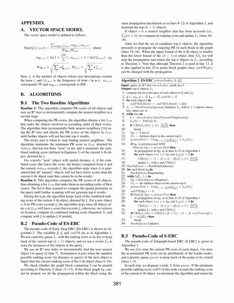
Algorithm 2 ES-EBC (rtreeIndex, k, Q)

Input: query Q, R*-tree rtreeIndex, result size kOutput: top-k objects Lr

1: compute the text relevance of each object to Q and ~uQ

2: ~q ← ~uQ, ~p ← ~0, Ld ← ~0, outPR ← ~03: for each object b do4: outPR(b.block) ← outPR(b.block) + ~q(b)5: Lr ← NewPriorityQueue(); Initialize Lr with k + 1 objects whose

key values are ∞6: while true do7: b ← rtreeIndex.NextNearestNeighbor(Q)8: Ld(b) ← Dist(Q, b)

9: if CRS(Lr(k)) ≤ β ∗ Ld(b)maxD

then10: break11: bgi ← b.block12: Os ← furthest object in the current top-k13: pruneDist ← λ log1−α

εoutPR(bgi)

+ Ld(Os)

14: if bgi is not processed ANDDist(Q, bgi) < pruneDist then

15: do propagation on bgi as in lines 8–23 of Algorithm 116: for each object o s.t. o ∈ bgi and Ld(o) > 0 do17: CRS(o) ← (1− β) ∗ (1− ~p(o)) + β ∗ Ld(o)

maxD18: update Lr with o and CRS(o)19: blockQueue← NewPriorityQueue()20: for each block bg do21: blockQueue.Enqueue(bg)22: while ‖~q‖1 ≥ ε do23: bgi = blockQueue.Dequeue()24: Os ← the furthest object in the current top-k25: pruneDist ← λ log1−α

εoutPR(bgi)

+ Ld(Os)

26: outPR(bgi) ← 027: if Dist(Q, bgi) < pruneDist then28: do propagation on bgi as in lines 8–23 of Algorithm 129: for each object o s.t. o ∈ bgi and Ld(o) > 0 do30: CRS(o) ← (1− β) ∗ (1− ~p(o)) + β ∗ Ld(o)

maxD31: update Lr with o and CRS(o)32: if CRS(Lr(k)) < CRS(Lr(k + 1))− (1− β) ∗ (α2max(~q) +

(1− α)‖~q‖1) then33: break;34: blockQueue.Update()

B.3 Pseudo-Code of S-EBCThe pseudo-code of Subgraph-based EBC (S-EBC) is given in

Algorithm 3.We use ~p to store the current PR score of each object, ~s to store

the accumulated PR score (to be distributed) of the border nodes,and a priority queue queue to keep track of the nodes to be visited(lines 1–3).

In each step, we dequeue a node X from queue. If the minimumpossible ranking score spRS of this node exceeds the ranking scoreof the current k-th object, we terminate the algorithm and return the

381

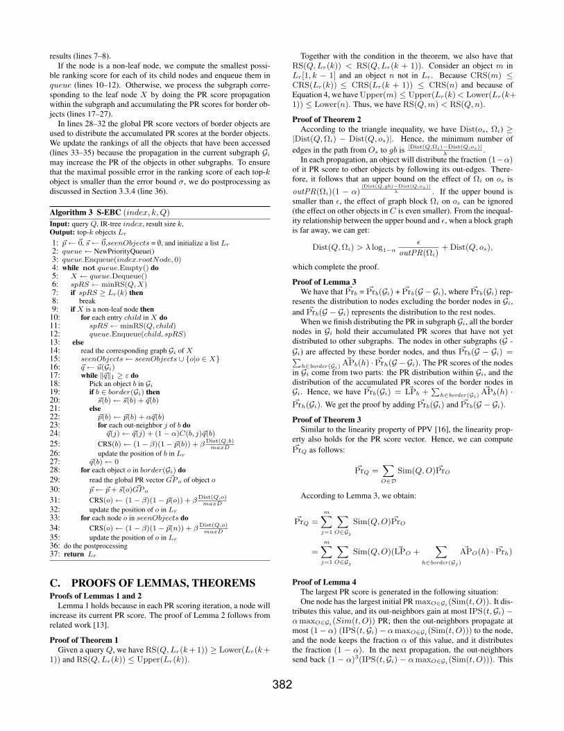
results (lines 7–8).If the node is a non-leaf node, we compute the smallest possi-

ble ranking score for each of its child nodes and enqueue them inqueue (lines 10–12). Otherwise, we process the subgraph corre-sponding to the leaf node X by doing the PR score propagationwithin the subgraph and accumulating the PR scores for border ob-jects (lines 17–27).

In lines 28–32 the global PR score vectors of border objects areused to distribute the accumulated PR scores at the border objects.We update the rankings of all the objects that have been accessed(lines 33–35) because the propagation in the current subgraph Gi

may increase the PR of the objects in other subgraphs. To ensurethat the maximal possible error in the ranking score of each top-kobject is smaller than the error bound σ, we do postprocessing asdiscussed in Section 3.3.4 (line 36).

Algorithm 3 S-EBC (index, k, Q)

Input: query Q, IR-tree index, result size k,Output: top-k objects Lr

1: ~p ← ~0, ~s ← ~0,seenObjects = ∅, and initialize a list Lr

2: queue ← NewPriorityQueue()3: queue.Enqueue(index.rootNode, 0)4: while not queue.Empty() do5: X ← queue.Dequeue()6: spRS ← minRS(Q, X)7: if spRS ≥ Lr(k) then8: break9: if X is a non-leaf node then

10: for each entry child in X do11: spRS ← minRS(Q, child)12: queue.Enqueue(child, spRS)13: else14: read the corresponding graph Gi of X15: seenObjects ← seenObjects ∪ o|o ∈ X16: ~q ← ~u(Gi)17: while ‖~q‖1 ≥ ε do18: Pick an object b in Gi

19: if b ∈ border(Gi) then20: ~s(b) ← ~s(b) + ~q(b)21: else22: ~p(b) ← ~p(b) + α~q(b)23: for each out-neighbor j of b do24: ~q(j) ← ~q(j) + (1− α)C(b, j)~q(b)

25: CRS(b) ← (1− β)(1− ~p(b)) + βDist(Q,b)

maxD26: update the position of b in Lr

27: ~q(b) ← 028: for each object o in border(Gi) do29: read the global PR vector ~GP o of object o

30: ~p ← ~p + ~s(o) ~GP o

31: CRS(o) ← (1− β)(1− ~p(o)) + βDist(Q,o)

maxD32: update the position of o in Lr

33: for each node o in seenObjects do34: CRS(o) ← (1− β)(1− ~p(n)) + β

Dist(Q,o)maxD

35: update the position of o in Lr

36: do the postprocessing37: return Lr

C. PROOFS OF LEMMAS, THEOREMSProofs of Lemmas 1 and 2

Lemma 1 holds because in each PR scoring iteration, a node willincrease its current PR score. The proof of Lemma 2 follows fromrelated work [13].

Proof of Theorem 1Given a query Q, we have RS(Q, Lr(k +1)) ≥ Lower(Lr(k +

1)) and RS(Q, Lr(k)) ≤ Upper(Lr(k)).

Together with the condition in the theorem, we also have thatRS(Q, Lr(k)) < RS(Q, Lr(k + 1)). Consider an object m inLr[1, k − 1] and an object n not in Lr . Because CRS(m) ≤CRS(Lr(k)) ≤ CRS(Lr(k + 1)) ≤ CRS(n) and because ofEquation 4, we have Upper(m) ≤ Upper(Lr(k) < Lower(Lr(k+1)) ≤ Lower(n). Thus, we have RS(Q, m) < RS(Q, n).

Proof of Theorem 2According to the triangle inequality, we have Dist(os, Ωi) ≥

|Dist(Q, Ωi) − Dist(Q, os)|. Hence, the minimum number ofedges in the path from Os to gb is |Dist(Q,Ωi)−Dist(Q,os)|

λ.

In each propagation, an object will distribute the fraction (1−α)of it PR score to other objects by following its out-edges. There-fore, it follows that an upper bound on the effect of Ωi on os is

outPR(Ωi)(1 − α)|Dist(Q,gb)−Dist(Q,os)|

λ . If the upper bound issmaller than ε, the effect of graph block Ωi on os can be ignored(the effect on other objects in C is even smaller). From the inequal-ity relationship between the upper bound and ε, when a block graphis far away, we can get:

Dist(Q, Ωi) > λ log1−α

ε

outPR(Ωi)+ Dist(Q, os),

which complete the proof.

Proof of Lemma 3We have that ~Prb = ~Prb(Gi) + ~Prb(G −Gi), where ~Prb(Gi) rep-

resents the distribution to nodes excluding the border nodes in Gi,and ~Prb(G − Gi) represents the distribution to the rest nodes.

When we finish distributing the PR in subgraph Gi, all the bordernodes in Gi hold their accumulated PR scores that have not yetdistributed to other subgraphs. The nodes in other subgraphs (G -Gi) are affected by these border nodes, and thus ~Prb(G − Gi) =∑

h∈border(Gi)~APb(h) · ~Prh(G −Gi). The PR scores of the nodes

in Gi come from two parts: the PR distribution within Gi, and thedistribution of the accumulated PR scores of the border nodes inGi. Hence, we have ~Prb(Gi) = ~LPb +

∑h∈border(Gi)

~APb(h) ·~Prh(Gi). We get the proof by adding ~Prb(Gi) and ~Prb(G − Gi).

Proof of Theorem 3Similar to the linearity property of PPV [16], the linearity prop-

erty also holds for the PR score vector. Hence, we can compute~PrQ as follows:

~PrQ =∑O∈D

Sim(Q, O) ~PrO

According to Lemma 3, we obtain:

~PrQ =

m∑j=1

∑O∈Gj

Sim(Q, O) ~PrO

=

m∑j=1

∑O∈Gj

Sim(Q, O)( ~LPO +∑

h∈border(Gj)

~APO(h) · ~Prh)

Proof of Lemma 4The largest PR score is generated in the following situation:One node has the largest initial PR maxO∈Gi(Sim(t, O)). It dis-

tributes this value, and its out-neighbors gain at most IPS(t,Gi)−α maxO∈Gi(Sim(t, O)) PR; then the out-neighbors propagate atmost (1− α) (IPS(t,Gi)− α maxO∈Gi(Sim(t, O))) to the node,and the node keeps the fraction α of this value, and it distributesthe fraction (1 − α). In the next propagation, the out-neighborssend back (1 − α)3(IPS(t,Gi) − α maxO∈Gi(Sim(t, O))). This

382

process continues until no PR needs to be propagated. The total PRthe node finally holds is:

maxLPr(t,Gi) = α maxO∈Gi

(Sim(t, O)) + α(((1− α) + ...+

(1− α)2n+1 + ...)(IPS(t,Gi)− α maxO∈Gi

(Sim(t, O))))

=α maxO∈Gi

(Sim(t, O))

+α ∗ (1− α)

1− (1− α)2(IPS(t,Gi)− α max

O∈Gi

(Sim(t, O))))

=1 + α− α2

2− αmaxO∈Gi

(Sim(t, O)) +1− α

2− αIPS(t,Gi)

Proof of Theorem 4According to Lemma 3, the largest PR score from the propaga-

tion within Gi is maxLPr(t,Gi).We next consider the effect of other subgraphs. The maximum

effect of subgraph Gj on Gi occurs if a certain border node in Gj

gets the initial prestige IPS(t,Gi). This is because all the effect ofGj on Gi is from border nodes. Each global PR vector of a bor-der node in Gj describes its effect on nodes in Gi. We find thelargest value from all the global PR vectors of border nodes, i.e.,maxbn∈border(Gj),b∈Gi

( ~Prbn(b)), and this is the maximum possi-ble PR that can be propagated from Gj to a node in Gi.

Combining the two parts completes the proof.

Proof of Lemma 5

IPS(Q,Gi) =∑

O∈Gi

Sim(Q, O)

=∑

O∈Gi

∑

t∈Q.ψ⋂

O.ψ

wQ.ψ,twO.ψ,t

WQ.ψWO.ψ

=∑

t∈Q.ψ⋂Gi.ψ

∑O∈Gi

wQ.ψ,twO.ψ,t

WQ.ψWO.ψ

=∑

t∈Q.ψ⋂Gi.ψ

wQ.ψ,t

WQ.ψ

∑O∈Gi

wO.ψ,t

WO.ψ

and we know Sim(t, O) =wt,twO.ψ,t

wt,tWO.ψ=

wO.ψ,t

WO.ψ, so:

IPS(Q,Gi) =∑

t∈Q.ψ⋂Gi.ψ

wQ.ψ,t

WQ.ψ

∑O∈Gi

Sim(t, O)

=∑

t∈Q.ψ⋂Gi.ψ

wQ.ψ,t

WQ.ψIPS(t,Gi)

Proof of Theorem 5Given any object o ∈ XO and any term t, it holds true that

maxGPr(t, X) ≥ Pr(t, o). Therefore,

maxPr(Q, X) =∑

t∈Q.ψ⋂

X.ψ

wQ.ψ,t

WQ.ψmaxGPr(t, X)

≥∑

t∈Q.ψ⋂

o.ψ

wQ.ψ,t

WQ.ψPr(t, o) = Pr(Q, o)

Proof of Theorem 6Given any object o ∈ XO, we know that maxPr(Q, X) ≥

Pr(Q, o), according to Theorem 5. Because o is contained in theregion X.Ω, we have Dist(Q.µ, X.Ω) ≤ Dist(Q, o). Hence weget minRS(Q, X) ≤ RS(Q, o).

Proof of Theorem 7It holds that the maximum possible effect of Gj on Gi is a factor

of maxbn∈border(Gj),b∈Gi( ~Prbn(b)). Multiplied by the total pres-

tige of Gj , we can get the maximum PR that Gj can propagate to anobject in Gi.

D. SUPPLEMENTARY EXPERIMENTS

D.1 Additional Dataset DetailsDataset GN is from the U.S. Board on Geographic Names (geon-

ames.usgs.gov). An object is a location with a geographic name.Dataset Web is generated from two datasets. One is WEBSPAM-UK20071 that consists of a large number of web documents; theother is a spatial dataset containing the tiger Census blocks in Iowa,Kansas, Missouri, and Nebraska (www.rtreeportal.org). We ran-domly combine web documents and spatial objects to get the Webdataset. Dataset Hotel contains spatial objects that represent hotelsin the US (www.allstays.com). Each object has a location and a setof words that describe the hotel (e.g., restaurant, pool).

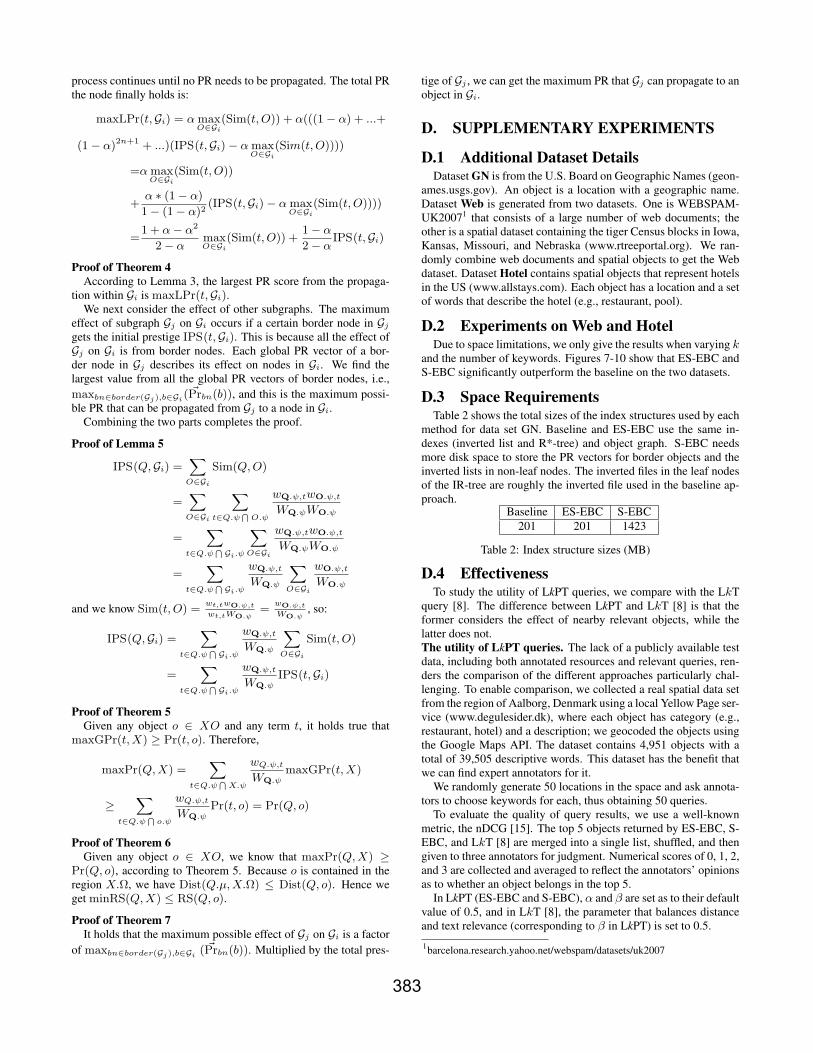
D.2 Experiments on Web and HotelDue to space limitations, we only give the results when varying k

and the number of keywords. Figures 7-10 show that ES-EBC andS-EBC significantly outperform the baseline on the two datasets.

D.3 Space RequirementsTable 2 shows the total sizes of the index structures used by each

method for data set GN. Baseline and ES-EBC use the same in-dexes (inverted list and R*-tree) and object graph. S-EBC needsmore disk space to store the PR vectors for border objects and theinverted lists in non-leaf nodes. The inverted files in the leaf nodesof the IR-tree are roughly the inverted file used in the baseline ap-proach.

Baseline ES-EBC S-EBC201 201 1423

Table 2: Index structure sizes (MB)

D.4 EffectivenessTo study the utility of LkPT queries, we compare with the LkT

query [8]. The difference between LkPT and LkT [8] is that theformer considers the effect of nearby relevant objects, while thelatter does not.The utility of LkPT queries. The lack of a publicly available testdata, including both annotated resources and relevant queries, ren-ders the comparison of the different approaches particularly chal-lenging. To enable comparison, we collected a real spatial data setfrom the region of Aalborg, Denmark using a local Yellow Page ser-vice (www.degulesider.dk), where each object has category (e.g.,restaurant, hotel) and a description; we geocoded the objects usingthe Google Maps API. The dataset contains 4,951 objects with atotal of 39,505 descriptive words. This dataset has the benefit thatwe can find expert annotators for it.

We randomly generate 50 locations in the space and ask annota-tors to choose keywords for each, thus obtaining 50 queries.

To evaluate the quality of query results, we use a well-knownmetric, the nDCG [15]. The top 5 objects returned by ES-EBC, S-EBC, and LkT [8] are merged into a single list, shuffled, and thengiven to three annotators for judgment. Numerical scores of 0, 1, 2,and 3 are collected and averaged to reflect the annotators’ opinionsas to whether an object belongs in the top 5.

In LkPT (ES-EBC and S-EBC), α and β are set as to their defaultvalue of 0.5, and in LkT [8], the parameter that balances distanceand text relevance (corresponding to β in LkPT) is set to 0.5.

1barcelona.research.yahoo.net/webspam/datasets/uk2007

383

1

10

100

1000

10000

100000

1e+006

1 10 20 30 40

Run

time

(mill

ion

sec.

)

top-k

BaselineES-EBC

S-EBC

Figure 7: Varying k (Web)

1

10

100

1000

10000

100000

1e+006

1 2 3 4

Run

time

(mill

ion

sec.

)

number of words

BaselineES-EBC

S-EBC

Figure 8: Varying # keywords(Web)

0

500

1000

1500

2000

1 10 20 30 40

Run

time

(mill

isec

onds

)

top-k

BaselineES-EBC

S-EBC

Figure 9: Varying k (Hotel)

0

500

1000

1500

2000

1 2 3 4

Run

time

(mill

isec

onds

)

number of words

BaselineES-EBC

S-EBC

Figure 10: Varying # keywords(Hotel)

Table 3 depicts the results. Both ES-EBC and S-EBC performsignificantly better than LkT queries that do not take into accountthe effects of nearby relevant objects. The approximate S-EBC al-gorithm performs slightly worse than ES-EBC.

ES-EBC S-EBC LkT [8]nDCG@5 0.8873 0.8524 0.7061

Table 3: Effectiveness of different algorithms

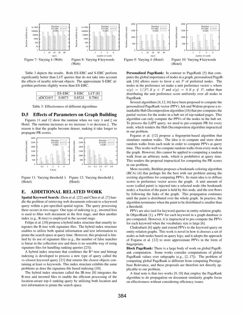
D.5 Effects of Parameters on Graph BuildingFigures 11 and 12 show the runtime when we vary λ and ξ on

Hotel. The runtime increases as we increase λ or decrease ξ. Thereason is that the graphs become denser, making it take longer topropagate PR scores.

0

500

1000

1500

2000

2500

3000

0.5 1 2 3 4

Run

time

(mill

isec

onds

)

λ (km)

BaselineES-EBC

S-EBC

Figure 11: Varying threshold λ(Hotel)

0

500

1000

1500

2000

2500

3000

0.1 0.3 0.5 0.7 0.9

Run

time

(mill

isec

onds

)

ξ

BaselineES-EBC

S-EBC

Figure 12: Varying threshold ξ(Hotel)

E. ADDITIONAL RELATED WORKSpatial Keyword Search: Zhou et al. [22] and Chen et al. [7] han-dle the problem of retrieving web documents relevant to a keywordquery within a pre-specified spatial region. The query processingthere occurs in two stages: One type of indexing (e.g., inverted list)is used to filter web document in the first stage, and then anotherindex (e.g., R-tree) is employed in the second stage.

Felipe et al. [10] propose a hybrid index structure that smartly in-tegrates the R-tree with signature files. The hybrid index structureenables to utilize both spatial information and text information toprune the search space at query time. However, this proposal is lim-ited by its use of signature files (e.g., the number of false matchesis linear in the collection size and there is no sensible way of usingsignature files for handling ranking queries [23]).

A hybrid index structure that combines the R*-tree and bitmapindexing is developed to process a new type of query called them-closest keyword query [21] that returns the closest objects con-taining at least m keywords. This index structure exhibits the sameproblems as does the signature-file based indexing [10].

The hybrid index structure called the IR-tree [8] integrates theR-tree and inverted files to enable the efficient processing of thelocation-aware top-k ranking query by utilizing both location andtext information to prune the search space.

Personalized PageRank: In contrast to PageRank [5] that com-putes the global importance of nodes in a graph, personalized PageR-ank [16] allows users to favor a set P of preferred nodes. Thenodes in the preference set make a unit preference vector u whereu(p) = 1/|P | if p ∈ P and u(p) = 0 if p /∈ P , rather thandistributing the unit preference score uniformly over all nodes inPageRank.

Several algorithms [4,12,16] have been proposed to compute thepersonalized PageRank vector (PPV). Jeh and Widom propose a re-markable Hub Decomposition algorithm [16] that pre-computes thepartial vectors for the nodes in a hub set of top-ranked pages. Thisalgorithm can only compute the PPVs of the nodes in the hub set.To process the LkPT query, we need to pre-compute PR for everynode, which renders the Hub Decomposition algorithm impracticalin our problem.

Fogaras et al. [12] propose a fingerprint-based algorithm thatsimulates random walks. The idea is to compute and store shortrandom walks from each node in order to compute PPVs at querytime. This works well to compute random walks from every node inthe graph. However, this cannot be applied to computing a randomwalk from an arbitrary node, which is prohibitive at query time.This renders the proposal impractical for computing the PR scoresin our problem.

More recently, Berkhin proposes a bookmark-coloring algorithm(BCA) [4] that perhaps fits the best with our problem among theexisting algorithms for computing PPVs. Its main idea is to diffusescores in preference vector across the graph. A unit amount ofscore (called paint) is injected into a selected node (the bookmarknode); a fraction of the paint is held by this node, and the rest flowsby following the links of the graph. This propagation continuesuntil the paint is distributed over the whole graph. In practice, thealgorithm terminates when the paint to be distributed is smaller thana threshold.

PPVs are also ised for keyword queries in entity-relation graphs.In ObjectRank [1], a PPV for each keyword in a graph database ispre-computed. However, it is impractical to pre-compute the PPVsfor each keyword when the vocabulary size is large [6].

Chakrabarti [6] apply and extend PPVs to the keyword query onentity-relation graphs. This work is novel in how it chooses a set ofnodes as hub nodes based on query logs; and it adopts the approachof Fogaras et al. [12] to store approximate PPVs in the form offingerprints.Block PageRank: There is a large body of work on global PageR-ank computation. Some works consider computations of globalPageRank values over subgraphs (e.g., [2, 17]). The problem ofcomputing global PageRank is different from computing Prestige-base Relevance, and these proposals are therefore not directly ap-plicable to our problem.

A final note is that two works [9, 18] that employ the PageRankalgorithm to do propagation on document similarity graphs focuson effectiveness without considering efficiency issues.

384