retrieving the vertical distribution of chlorophyll a ... · readme figure s1 figure s2 figure s3...

RESEARCH ARTICLE10.1002/2014JC010355

Retrieving the vertical distribution of chlorophyll aconcentration and phytoplankton community compositionfrom in situ fluorescence profiles: A method based on a neuralnetwork with potential for global-scale applicationsR. Sauzede1,2, H. Claustre1,2, C. Jamet3, J. Uitz1,2, J. Ras1,2, A. Mignot4, and F. D’Ortenzio1,2

1Laboratoire d’Oc�eanographie de Villefranche, CNRS, UMR7093, Villefranche-Sur-Mer, France, 2Universit�e Pierre et MarieCurie-Paris 6, UMR7093, Laboratoire d’oc�eanographie de Villefranche, Villefranche-Sur-Mer, France, 3Laboratoired’Oc�eanologie et de G�eosciences, UMR8187, ULCO/CNRS, Wimereux, France, 4Department of Earth, Atmospheric andPlanetary Sciences, Massachusetts Institute of Technology, Cambridge, Massachusetts, USA

Abstract A neural network-based method is developed to assess the vertical distribution of (1) chlorophylla concentration ([Chl]) and (2) phytoplankton community size indices (i.e., microphytoplankton, nanophyto-plankton, and picophytoplankton) from in situ vertical profiles of chlorophyll fluorescence. This method (FLA-VOR for Fluorescence to Algal communities Vertical distribution in the Oceanic Realm) uses as input only theshape of the fluorescence profile associated with its acquisition date and geo-location. The neural network istrained and validated using a large database including 896 concomitant in situ vertical profiles of High-Performance Liquid Chromatography (HPLC) pigments and fluorescence. These profiles were collected during22 oceanographic cruises representative of the global ocean in terms of trophic and oceanographic condi-tions, making our method applicable to most oceanic waters. FLAVOR is validated with respect to the retrievalof both [Chl] and phytoplankton size indices using an independent in situ data set and appears to be relativelyrobust spatially and temporally. To illustrate the potential of the method, we applied it to in situ measure-ments of the BATS (Bermuda Atlantic Time Series Study) site and produce monthly climatologies of [Chl] andassociated phytoplankton size indices. The resulting climatologies appear very promising compared to clima-tologies based on available in situ HPLC data. With the increasing availability of spatially and temporally well-resolved data sets of chlorophyll fluorescence, one possible global-scale application of FLAVOR could be todevelop 3-D and even 4-D climatologies of [Chl] and associated composition of phytoplankton communities.The Matlab and R codes of the proposed algorithm are provided as supporting information.

1. Introduction

Phytoplankton is an essential component in marine biogeochemical cycles and ecosystems. The assessmentof its spatio-temporal distribution and variability across the global ocean is thus an important objective inbiological oceanography. Methods have been developed for monitoring oceanic phytoplankton distribution(horizontally and vertically) with the objective to continuously increase the spatio-temporal resolution ofdata acquisition. These methods often rely on the estimation of the chlorophyll a concentration which is auniversal proxy for phytoplankton biomass. Remote sensing of Ocean Color Radiometry (OCR) offers aunique way to map quasi-synoptically chlorophyll a concentration at the ocean surface. Through this tech-nique, a wide range of applications has been developed, leading to a better understanding of phytoplank-ton dynamics in the upper ocean [McClain, 2009; Siegel et al., 2013]. However, the use of remote sensing ofOCR provides chlorophyll a concentration only for the surface layers of the ocean [Gordon and McCluney,1975], representing one-fifth of the so-called euphotic layer where phytoplankton photosynthesis takesplace [Morel and Berthon, 1989]. The vertical distribution of phytoplankton thus escapes from this remotedetection. While in situ vertical profiles of chlorophyll a concentration are determined with the best accu-racy by high-performance liquid chromatography (HPLC) [Claustre et al., 2004; Peloquin et al., 2013], thismethod is not compatible with highly repetitive measurements.

Introduced by Lorenzen [1966], measurement of in vivo fluorescence of chlorophyll a is a nonintrusive tech-nique that allows the direct in situ assessment of chlorophyll a concentration. Besides the dissolved oxygen,

Key Points:� Chlorophyll a concentration is

retrieved from fluorescence profiles� Phytoplankton communities size

indices are retrieved fromfluorescence profiles� A neural network is developed with a

potential for global-scale applications

Supporting Information:� Readme� Figure S1� Figure S2� Figure S3� Figure S4� Figure S5� Figure S6� Figure S7� R and Matlab codes of the proposed

algorithm

Correspondence to:R. Sauzede,[email protected]

Citation:Sauzede, R., H. Claustre, C. Jamet,J. Uitz, J. Ras, A. Mignot, andF. D’Ortenzio (2015), Retrieving thevertical distribution of chlorophyll aconcentration and phytoplanktoncommunity composition from in situfluorescence profiles: A method basedon a neural network with potential forglobal-scale applications, J. Geophys.Res. Oceans, 120, doi:10.1002/2014JC010355.

Received 30 JUL 2014

Accepted 17 DEC 2014

Accepted article online 5 JAN 2015

SAUZ�EDE ET AL. VC 2015. American Geophysical Union. All Rights Reserved. 1

Journal of Geophysical Research: Oceans

PUBLICATIONS

http://dx.doi.org/10.1002/2014JC010355

http://onlinelibrary.wiley.com/journal/10.1002/(ISSN)2169-9291/

http://publications.agu.org/

chlorophyll a fluorescence is certainly the most measured biogeochemical property in the global ocean.The in vivo fluorescence of chlorophyll a can be considered as a proxy for chlorophyll a concentration withsome unavoidable limitations such as the variability of the fluorescence-to-chlorophyll a concentration ratioas a function of physiological constraints or community composition [Kiefer, 1973; Falkowski et al., 1985;Cunningham, 1996]. While in vivo fluorescence is an imperfect proxy, it presents the advantage that it canbe easily measured thanks to miniature in situ sensors. Thus, the inherent weaknesses of fluorometric meas-urements are largely compensated by their cost effective acquisition that enables numerous data to begathered. This is now especially true considering that, besides oceanic cruises, in vivo fluorescence is acces-sible through autonomous platforms (floats, gliders, animals), allowing a global fluorescence database to beprogressively assembled [Claustre et al., 2010a, 2010b].

On a case-by-case basis (e.g., an oceanographic cruise), a fluorescence database can be easily and accu-rately converted into a chlorophyll a concentration database, for example, thanks to simultaneous HPLCdetermination [Claustre et al., 1999]. However, with the goal of developing large-scale chlorophyll a concen-tration databases from the merging of different fluorescence data from diverse origins (e.g., sensors, plat-forms), their consistency and interoperability will become a critical issue. First, the expected exponentialgrowth of fluorescence profile acquisition in the near future (more and more autonomous platforms will bedeployed) will stimulate regular updates of these ‘‘super’’ databases. Hence, methods have to systematicallyadd new data in a way that does not compromise the reliability and the quality of the existing database.Second, as some platforms (e.g., floats, animals) are not necessarily recovered, the initial sensor calibration,if any, would represent the only reference for the whole acquisition period (sometimes extending over sev-eral years). This can represent a bias because these platforms acquire fluorescence profiles in conditionswhere the phytoplankton communities and their physiological state may have drastically changed in com-parison to the conditions prevailing at the time of platform deployment and initial sensor calibration.Robust methods that allow the retrieval of chlorophyll a concentration from fluorescence measurementswithout any regular or simultaneous HPLC measurement will need to be developed.

Several alternative methods have already been proposed for calibrating fluorescence profiles, whichpartly circumvent the above mentioned issues. Lavigne et al. [2012] use the satellite remotely detectedsurface chlorophyll a concentration as a way to scale the whole fluorescence vertical profile to this ref-erence surface value. While this method presents the advantage of allowing the interoperability of datasets from different origins and locations, it is obviously not applicable to situations where no concurrentsatellite data are available (SeaWiFS was launched in 1997). Furthermore, it implicitly postulates that thesatellite-derived surface chlorophyll a concentration is the ‘‘accurate’’ reference, an assumption that canbe challenged, especially in some oceanic regions [e.g., Bricaud et al., 2002; Johnson et al., 2013]. Mignotet al. [2011] have shown that information related to chlorophyll a concentration is embedded in theshape of the fluorescence profile. For example, it is intuitive that the deeper the Deep Chlorophyll maxi-mum (DCM), the lower the surface chlorophyll a concentration [see also, Morel and Bertrhon, 1989; Uitzet al., 2006]. Mignot et al. [2011] thus proposed a calibration of the fluorescence profile based on itsshape. The prerequisite of the method is that the profile shape has to be a priori categorized eitherinto a stratified type (modeled by a Gaussian) or a mixed type (modeled by a sigmoid). Clearly, theadvantage of this method is that it does not require any complementary information. Its limit lies in theneed for an initial classification of the fluorescence profiles, which may be complicated for those thatdo not clearly belong to one of the two categories.

The primary objective of the present study relies on, and further extends, the approach of Mignot et al.[2011]. It aims at developing a self-consistent calibration method of the fluorescence profile essentiallybased on its shape, and which requires minimum additional information or a priori knowledge. The choiceof limiting the use of additional information is essentially guided by the long-term objective of this study,which is to reconcile the oldest databases (assembled during the 1970s when the first fluorescence profileswere recorded with no or scarce ancillary data) with the most recent as well as future databases (derivedfrom autonomous platforms). Besides the fluorescence profile, its geo-location represents robust additionalinformation that is systematically present (as metadata) and potentially useful. At first order (e.g., on aglobal scale), the geo-location indeed intrinsically embeds information relative to the trophic status(amount of biomass, e.g., spring bloom in the North Atlantic) or hydrographic conditions (stratified versusmixed, e.g., subtropical gyres versus upwellings).

Journal of Geophysical Research: Oceans 10.1002/2014JC010355


Artificial neural networks (ANNs) are approximate functions of any data sets [Marzban, 2009]. They representpowerful methods to develop models especially when the underlying relationships are unknown, which istypically the case here with the fluorescence profile shape and the chlorophyll a concentration. In particular,multilayered perceptrons (MLPs) are universal approximators of any differentiable and continuous function[Hornik et al., 1989] which are well adapted to ecological data sets having often nonlinear spatially and tem-porally complex and noisy distributions [Lek and Gu�egan, 1999]. In oceanography, such methods have beendeveloped and used for the retrieval of various products such as the diffuse attenuation coefficient [Jametet al., 2012], the partial pressure of carbon dioxide (pCO2) surface distribution [Friedrich and Oschlies, 2009;Telszewski et al., 2009], the surface phytoplankton pigment concentration [Gross et al., 2000] or the surfacephytoplankton functional types [Bricaud et al., 2007; Raitsos et al., 2008; Ben Mustapha et al., 2013; Palaczet al., 2013]. These methods thus appear well adapted to the type of problem identified here, i.e., theretrieval of a calibrated chlorophyll a concentration profile from the shape and geo-location of a fluores-cence profile.

In most studies dealing with the possible impact of environmental changes on oceanic carbon fluxes, thenature of phytoplankton communities (e.g., performing regenerated versus new production, small versuslarge phytoplankton) is an essential variable to account for [e.g., Le Quere et al., 2005]. Ongoing efforts areunderway to synthesize the historical knowledge on phytoplankton taxonomy in gathered databases [e.g.,Buitenhuis et al., 2012; Leblanc et al., 2012]. These data sets, nevertheless, remain rather sparse and the possi-bility to regularly improve and update them is weak simply because there are less taxonomic experts thanbefore. Alternative procedures thus need to be developed. Uitz et al. [2006] have shown that phytoplanktonsize indices can be derived from High-Performance Liquid Chromatography (HPLC) pigment analysis [seealso Peloquin et al., 2013]. These indices can be related to surface chlorophyll a concentration, so thatexplicit relationships can be observed between the phytoplankton biomass (e.g., chlorophyll a concentra-tion), the phytoplankton communities (e.g., phytoplankton size indices) and their vertical distribution.

In summary, the twofold objective of the present study is to retrieve, from the sole knowledge of the fluo-rescence profile shape and geo-location, the vertical profile of (1) chlorophyll a concentration and (2) phyto-plankton community size indices. To address this objective, we developed a MLP-based method, hereafterreferred to as FLAVOR for Fluorescence to Algal communities Vertical distribution in the Oceanic Realm. TheMLP is trained and validated using an in situ database that contains 896 continuous vertical fluorescence

Figure 1. Geographic distribution of the 896 stations used in the present study. For these stations, sampling for HPLC pigment was simultaneous to the acquisition of the fluorescence profile.



profiles acquired simultaneously to HPLC pigment determinations at selected depths. This database is rep-resentative of the range of trophic and oceanographic conditions prevailing in the global open ocean.Therefore, we expect that any potential conclusion of the present study will be of general applicability tothe global ocean.

2. Data Presentation and Processing

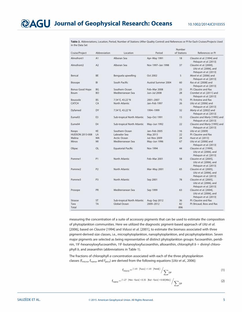
2.1. Database of Vertical Profiles of Chlorophyll Fluorescence and HPLC PigmentsThe present study makes use of an extensive database of concurrent vertical profiles of chlorophyll fluores-cence (fluo, see abbreviations in Table 1) and phytoplankton pigments determined by HPLC. This data set isan extension of the one used by Mignot et al. [2011]. The data were collected at 896 stations sampled dur-ing 22 open ocean cruises between 1991 and 2012 (Table 2), which took place in a wide variety of oceanicregions. Most of the data were collected in the Mediterranean Sea (39%) and the Atlantic Ocean (36%), 17%of the data are from the Pacific Ocean, 3% from the South Ocean, 3% from the Arctic Ocean, and 2% fromthe Indian Ocean (Figure 1).

The chlorophyll a in vivo fluorescence profiles acquired during the 22 cruises were obtained using a fluo-rometer mounted on a CTD-rosette. We applied a quality control to each fluorescence profile similarly toD’Ortenzio et al. [2010] in order to remove aberrant data caused by electronic noise.

Samples for HPLC pigment determinations were acquired at discrete depths (approximately 10 data pointsper profile) and analyzed according to the method described by Claustre [1994] for the EUMELI cruises,Vidussi et al. [1996] for the cruises that occurred prior to 2004, and Ras et al. [2008] for all other cruises after2004. The concentration of total chlorophyll a as determined by HPLC actually refers to the concentrationof the so-called total chlorophyll a ([TChl]) which is the sum of the concentrations of monovinyl-chlorophylla, divinyl-chlorophyll a, chlorophyllide a and the allomeric and epimeric forms of chlorophyll a. [TChl] is anestimate of the total phytoplankton biomass. In addition to chlorophyll a, the HPLC technique enables

Table 1. Abbreviations Used in the Present Study and Their Significance

Abbreviations Significance

[TChl] Chlorophyll a concentration associated to the total phytoplankton biomass (mg m23)fmicro Fraction of chlorophyll a associated to microphytoplanktonfnano Fraction of chlorophyll a associated to nanophytoplanktonfpico Fraction of chlorophyll a associated to picophytoplankton[microChl] Total chlorophyll a concentration associated to microphytoplankton (mg m23)[nanoChl] Total chlorophyll a concentration associated to nanophytoplankton (mg m23)[picoChl] Total chlorophyll a concentration associated to picophytoplankton (mg m23)[Chl] Chlorophyll a concentration (mg m23) referring either to [TChl] or [microChl], [nanoChl], and [picoChl]½TChl�Z0

[TChl] integrated from the surface up to the depth Z0 (mg m22)z Geometrical depth (m)Z0 Depth at which the fluorescence begins to be constant with depth (m)Ze Euphotic layer depth (m)Zm Mixed layer depth (m)f Depth normalized with respect to Z0, f5z=Z0, dimensionlessFuco Fucoxanthin (mg m23)Perid Peridinin (mg m23)Hex-fuco 190-Hexanoyloxyfucoxanthin (mg m23)But-fuco 190-Butanoyloxyfucoxanthin (mg m23)Allo Alloxanthin (mg m23)TChlb Chlorophyll b 1 divinyl Chlorophyll b (mg m23)Zea Zeaxanthin (mg m23)Lon Longitude (�E)Day Day of the yearLonrad Longitude transformed in radiansDayrad Day transformed in radiansfluo The fluorescence (relative units)fluonorm The normed fluorescence (dimensionless)[Chl]HPLC The [Chl] values of reference estimated by HPLC (mg m23)[Chl]MLP The 10 discrete values of [Chl] returned by the MLP (mg m23)[Chl]cal The fluorescence profile calibrated in [Chl] (mg m23)a The calibration coefficient, such as ½TChl�cal5 a : fluoMAPD Median absolute percent difference (%)a The slope of the linear regression between [Chl]MLP or [Chl]cal and the reference values of [Chl] estimated by HPLC



measuring the concentration of a suite of accessory pigments that can be used to estimate the composition

of phytoplankton communities. Here we utilized the diagnostic pigment-based approach of Uitz et al.

[2006], based on Claustre [1994] and Vidussi et al. [2001], to estimate the biomass associated with three

pigment-derived size classes, i.e., microphytoplankton, nanophytoplankton, and picophytoplankton. Seven

major pigments are selected as being representative of distinct phytoplankton groups: fucoxanthin, peridi-

nin, 190-hexanoyloxyfucoxanthin, 190-butanoyloxyfucoxanthin, alloxanthin, chlorophyll b 1 divinyl chloro-

phyll b, and zeaxanthin (abbreviations in Table 1).

The fractions of chlorophyll a concentration associated with each of the three phytoplanktonclasses (fmicro, fnano, and fpico) are derived from the following equations [Uitz et al., 2006]:

fmicro5 1:41 Fuco½ �11:41 Perid½ �ð Þ.X

DP(1)

fnano5 1:27 Hex2fuco½ �10:35 But2fuco½ �10:60½Allo�ð Þ.X

DP(2)

Table 2. Abbreviations, Location, Period, Number of Stations (After Quality Control) and References or PI for Each Cruises/Projects Usedin the Data Set

Cruise/Project Abbreviation Location PeriodNumber

of Stations References or PI

Almofront1 A1 Alboran Sea Apr–May 1991 18 Claustre et al. [1994] andPeloquin et al. [2013]

Almofront2 A2 Alboran Sea Nov 1997–Jan 1998 37 Claustre et al. [2000],Uitz et al. [2006], andPeloquin et al. [2013]

Bencal BE Benguela upwelling Oct 2002 5 Morel et al. [2006] andPeloquin et al. [2013]

Biosope BI South Pacific Austral Summer 2004 60 Ras et al. [2008] andPeloquin et al. [2013]

Bonus Good Hope BG Southern Ocean Feb–Mar 2008 23 PI: Claustre and RasBoum BO Mediterranean Sea Jun–Jul 2008 28 Crombet et al. [2011] and

Peloquin et al. [2013]Boussole BS 7.54�E, 43.22�N 2001–2007 75 PI: Antoine and RasCATCH CA North Atlantic Jan–Feb 1997 26 Uitz et al. [2006] and

Peloquin et al. [2013]Dyfamed DY 7.54�E, 43.22�N 1994–1999 32 Marty et al. [2002] and

Peloquin et al. [2013]Eumeli3 E3 Sub-tropical North Atlantic Sep–Oct 1991 15 Claustre and Marty [1995] and

Peloquin et al. [2013]Eumeli4 E4 Sub-tropical North Atlantic May–Jun 1992 22 Claustre and Marty [1995] and

Peloquin et al. [2013]Keops KE Southern Ocean Jan–Feb 2005 16 Uitz et al. [2009]HUDSON 2013-008 LA Labrador Sea May 2013 22 PI: Claustre and RasMalina MA Arctic Ocean Jul–Nov 2009 24 Huot et al. [2013]Minos MI Mediterranean Sea May–Jun 1996 67 Uitz et al. [2006] and

Peloquin et al. [2013]Olipac OL Equatorial Pacific Nov 1994 44 Claustre et al. [1999],

Uitz et al. [2006], andPeloquin et al. [2013]

Pomme1 P1 North Atlantic Feb–Mar 2001 58 Claustre et al. [2005],Uitz et al. [2006], andPeloquin et al. [2013]

Pomme2 P2 North Atlantic Mar–May 2001 65 Claustre et al. [2005],Uitz et al. [2006], andPeloquin et al. [2013]

Pomme3 P3 North Atlantic Sep 2001 78 Claustre et al. [2005],Uitz et al. [2006], andPeloquin et al. [2013]

Prosope PR Mediterranean Sea Sep 1999 63 Claustre et al. [2004],Uitz et al. [2006], andPeloquin et al. [2013]

Strasse ST Sub-tropical North Atlantic Aug–Sep 2012 36 PI: Claustre and RasTara TA Global Ocean 2009–2012 82 PI: Bricaud, Boss and RasTotal 896



fpico5 1:01 TChlb½ �10:86 Zea½ �ð Þ.X

DP(3)

withX

DP representing the sum of the seven diagnostic pigments concentrations:X

DP51:41 Fuco½ �11:41 Perid½ �11:27 Hex2fuco½ �10:35 But2fuco½ �10:60 Allo½ �11:01 TChlb½ �10:86½Zea�(4)

It is then possible to derive the chlorophyll a concentration associated with each of the three phytoplanktonclasses ([microChl], [nanoChl], and [picoChl]) according to the following equations:

microChl½ �5 fmicro�½TChl� (5)

nanoChl½ �5 fnano�½TChl� (6)

picoChl½ �5 fpico�½TChl� (7)

The pigment-based approach of Uitz et al. [2006], admittedly, has some limitations. For example,some diagnostic pigments are shared by several phytoplankton groups and some groups may covera broad size range. Nevertheless, it has proven valuable at regional and global scales for apprehend-ing the composition of phytoplankton assemblages, both in terms of taxonomic composition andsize structure. Recently, some modifications to the Uitz et al. [2006] approach have been proposed[Brewin et al., 2010; Devred et al., 2011]. Yet, in a comparative study, Brewin et al. [2014] show thatthese modifications do not bring major changes to the pigment-derived size structure of phytoplank-ton communities. Hence, in the present study, we calculate the [microChl], [nanoChl], and [picoChl]following Uitz et al. [2006].

Finally, a quality control was applied to each HPLC-determined vertical pigment profile as described in Uitzet al. [2006], i.e., (1) samples with [TChl] lower than 0.001 mg m23 were rejected, (2) the first sample has tobe located between the surface and 10 m depth, (3) the last sample has to be taken at a depth greater orequal to the euphotic depth, Ze, defined as the depth at which the irradiance is reduced to 1% of its surfacevalue, and (4) a minimum of four samples per profile is required. For this quality control procedure, Ze isestimated according to the method of Morel and Berthon [1989], by using the [TChl] profile derived fromHPLC estimates.

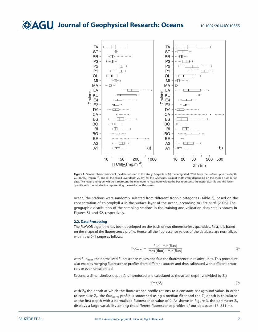
The data set used in this study includes concurrent fluorescence vertical profiles and HPLC-determined [TChl], [microChl], [nanoChl], and [picoChl] at discrete depths. This data set is represen-tative of a large variety of hydrological, biogeochemical and associated trophic conditions observedin the open ocean (Figure 2). First, the HPLC-fluorescence database is characteristic of a broad vari-ety of hydrological conditions. For example, it includes measurements acquired in the North Atlanticduring winter when the mixed layer depth may reach 700 m (CATCH cruise) as well as measure-ments from the Subtropical South Pacific Gyre when the average mixed layer depth in spring is�30 m (BIOSOPE cruise). Second, the database is representative of most trophic conditions (fromoligotrophic to eutrophic waters) observed in the global ocean. The parameter TChl½ �Z0

defined asthe [TChl] integrated between the surface and the depth Z0 describes these different trophic condi-tions. Z0 is set as the depth at which the fluorescence profile returns to a constant backgroundvalue (see Figures 3a and 3b and section 2.2 for the calculation details). Indeed, the data setappears to be representative of the global ocean as TChl½ �Z0

covers 2 order of magnitude. The mostoligotrophic conditions were found during the Malina cruise in the Arctic Ocean with a value ofabout 10 mg m22; similarly, the TChl½ �Z0

minimum value measured during the BIOSOPE cruise is18 mg m22. The most eutrophic conditions are also represented with some profiles acquired in theLabrador Sea during the spring bloom with TChl½ �Z0

values of about 900 mg m22. Because our dataset is representative of a broad variety of conditions, we expect that the method developed herewill be applicable at a global scale in the open ocean.

The data set presented here was split into two subsets. One subset was used for training the MLP;the second data set was used for validating the MLP. These two independent data sets, respectively,including about 80% (717 profiles) and 20% (179 profiles) of the initial data set, were randomly builtup from a random selection of stations. As both data sets should be representative of the open



ocean, the stations were randomly selected from different trophic categories (Table 3), based on theconcentration of chlorophyll a in the surface layer of the ocean, according to Uitz et al. [2006]. Thegeographic distribution of the sampling stations in the training and validation data sets is shown inFigures S1 and S2, respectively.

2.2. Data ProcessingThe FLAVOR algorithm has been developed on the basis of two dimensionless quantities. First, it is basedon the shape of the fluorescence profile. Hence, all the fluorescence values of the database are normalizedwithin the 0–1 range as follows:

fluonorm5fluo2minðfluoÞ

max fluoð Þ2minðfluoÞ (8)

with fluonorm the normalized fluorescence values and fluo the fluorescence in relative units. This procedurealso enables merging fluorescence profiles from different sources and thus calibrated with different proto-cols or even uncalibrated.

Second, a dimensionless depth, f, is introduced and calculated as the actual depth, z, divided by Z0:

f5z=Z0 (9)

with Z0 the depth at which the fluorescence profile returns to a constant background value. In orderto compute Z0, the fluonorm profile is smoothed using a median filter and the Z0 depth is calculatedas the first depth with a normalized fluorescence value of 0. As shown in Figure 3, the parameter Z0

displays a large variability among the different fluorescence profiles of our database (17–831 m).

Figure 2. General characteristics of the data set used in this study. Boxplots of (a) the integrated [TChl] from the surface up to the depthZ0, [TChl]Z0 (mg m22), and (b) the mixed layer depth Zm (m) for the 22 cruises. Boxplot widths vary depending on the cruise’s number ofdata. The lower and upper whiskers represent the minimum to maximum values; the box represents the upper quartile and the lowerquartile with the middle line representing the median of the values.



Scaling the fluorescence profiles with respect to f enables to merge all profiles regardless of theirvertical shape and range of variation, simultaneously accounting for their variability. This normal-ization is an essential step because the MLP can only use as input discrete fluorescence valuestaken at fixed depths. Figure 3 shows three schematic examples of fluorescence profile, either non-normalized (Figure 3a) or depth-normalized (Figure 3b), obtained from contrasted open oceanenvironments, i.e., a typical profile of deep winter-mixing conditions (red curve), a profile with aDeep Chlorophyll Maximum (DCM) characteristic of stratified oligotrophic systems (green curve),and a profile with a subsurface maximum that can be encountered in mesotrophic or eutrophicenvironments with a relatively shallow mixed layer (blue curve). Based on the examination of Fig-ure 3, it appears that, if the profile is not scaled with respect to depth, the 10 fixed-depth data

Z0 (m)

Fre

quen

cy

0 200 400 600 800

010

2030

4050

6070

c)

Figure 3. Characteristics of the fluorescence profile shape. (a) Three schematic normalized fluorescence profiles representative ofthe diversity of the observed situations; red: deeply mixed profile; green: stratified profile; blue: shallow mixed profile. Notethat the corresponding Z0 depths are reported. The lines correspond to the fluorescence profiles while the dots identify thehypothetical inputs of the fluorescence profiles for the MLP (10 inputs). (b) Same as for Figure 3a expect that the geometricaldepth is here replaced by the dimensionless depth f. (c) Histogram of the Z0 frequency distribution for the 896 fluorescence pro-files of the database.



points used as input to the MLP may not account for all the verti-cal variability of the fluorescence profile.

3. FLAVOR Algorithm Development

In the following, [Chl] refers either to the chlorophyll a concentrationassociated with the total phytoplankton biomass ([TChl]) or with themicrophytoplankton, nanophytoplankton, and picophytoplankton([microChl], [nanoChl], and [picoChl], respectively).

Our proposed FLAVOR algorithm is based on an Artificial Neural Net-work (ANN). It uses as input data a normalized in situ vertical fluores-cence profile along with the corresponding geo-location and date toretrieve vertical profiles of chlorophyll a associated with the total phyto-plankton biomass ([TChl]) and with three phytoplankton size classes([microChl], [nanoChl], and [picoChl]). FLAVOR is a two-step calibration

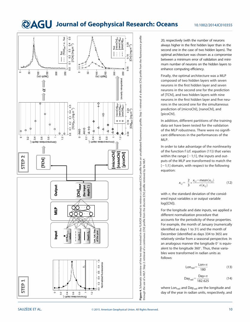
method, as shown on the flowchart in Figure 4. First, a discrete (10-point) profile of [Chl] ([Chl]MLP) is derivedfrom an in situ fluorescence profile based on an ANN. The second step of the method consists in returninga quasi-continuous profile of [Chl] (i.e., with a vertical resolution identical as that of the in situ fluorescenceprofile, [Chl]cal) based on the discrete ANN-derived [Chl] profile. This second step differs depending on theproduct to be returned by the ANN ([TChl] or [microChl], [nanoChl] and [picoChl]). Two different ANN-basedalgorithms are developed for inferring vertical profiles of either (1) [TChl] or (2) simultaneously [microChl],[nanoChl], and [picoChl].

3.1. Principles of Multilayer Perceptron (MLP)The ANN used in this study is a Multilayered Perceptron (MLP) [Bishop, 1995] composed of four layers:one input layer, two hidden layers, and one output layer. In each layer, the neurons, which are elemen-tary transfer functions, are interconnected with the neurons of the preceding and following layers byweights. The transfer of information through the MLP is done between the inputs I and outputs o andcan be described as:

o5fðw2;o f w1;2 f wi;1 I� ��

Þ (10)

with f a sigmoid nonlinear function:

f xð Þ5a� exp a:xð Þ21exp a:xð Þ11

(11)

where a and a are two constants. In equation (10), wi,1, w1,2, and w2,o are the weight matrices that describethe connections between the input and first hidden layers, the first and second hidden layers, and the secondhidden layer and the output layer, respectively. The coefficients of the weight matrix are iteratively readjustedduring the training of the MLP in order to minimize a cost function defined as the quadratic differencebetween the desired and computed outputs. To this end, we used the back-propagation conjugate-gradienttechnique [Hornik et al., 1989; Bishop, 1995], which is an iterative optimization method particularly adapted toMLPs. The training data set (80% of the entire initial data set) is further randomly split into two subdata sets(50% each), the so-called ‘‘learning’’ and ‘‘test’’ data sets. During the training process, these two subsets ofdata are used to cross validate the MLP and prevent from overlearning [Bishop, 1995]. Eventually, the valida-tion data set used to evaluate the performance of the MLP is composed of 20% of the entire initial database.

3.2. Application of the MLP to the Chlorophyll Fluorescence and HPLC Pigment DatabaseMultiple tests were carried out to identify the optimal combination of input and output parameters which yieldthe best MLP performance. We selected the final following set of parameters as inputs (see also Figure 4): (1) 10data points from the normalized fluorescence profile taken at regular intervals between the dimensionless depths0 and 1.3; (2) the depth Z0; (3) the dimensionless depth f at which [Chl] is to be computed; and (4) the location(latitude and longitude) and acquisition date (day of the year) of the considered fluorescence profile. Several testswere also performed to determine the optimal architecture of the MLP. Two types of architecture were tested:one or two hidden layers with a number of neurons in each layer varying between 1 and 50 and between 1 and

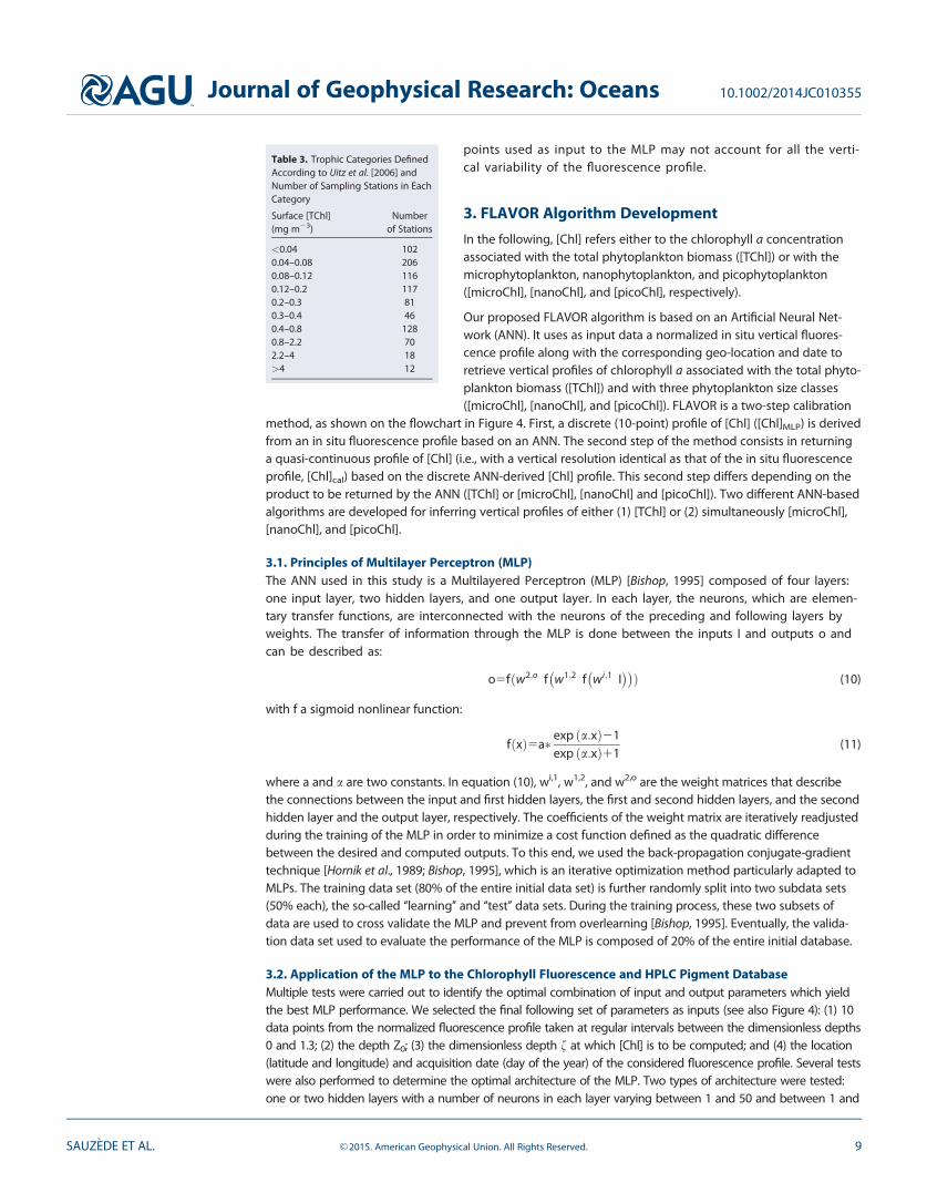
Table 3. Trophic Categories DefinedAccording to Uitz et al. [2006] andNumber of Sampling Stations in EachCategory

Surface [TChl](mg m23)

Numberof Stations

<0.04 1020.04–0.08 2060.08–0.12 1160.12–0.2 1170.2–0.3 810.3–0.4 460.4–0.8 1280.8–2.2 702.2–4 18>4 12



20, respectively (with the number of neuronsalways higher in the first hidden layer than in thesecond one in the case of two hidden layers). Theoptimal architecture was chosen as a compromisebetween a minimum error of validation and mini-mum number of neurons on the hidden layers toenhance computing efficiency.

Finally, the optimal architecture was a MLPcomposed of two hidden layers with sevenneurons in the first hidden layer and sevenneurons in the second one for the predictionof [TChl], and two hidden layers with nineneurons in the first hidden layer and five neu-rons in the second one for the simultaneousprediction of [microChl], [nanoChl], and[picoChl].

In addition, different partitions of the trainingdata set have been tested for the validationof the MLP robustness. There were no signifi-cant differences in the performances of theMLP.

In order to take advantage of the nonlinearityof the function f (cf. equation (11)) that varieswithin the range [21;1], the inputs and out-puts of the MLP are transformed to match the[21;1] domain, with respect to the followingequation:

xi;j523� xi;j2meanðxi;jÞ

rðxi;jÞ(12)

with r, the standard deviation of the consid-ered input variables x or output variablelog([Chl]).

For the longitude and date inputs, we applied adifferent normalization procedure thataccounts for the periodicity of these properties.For example, the month of January (numericallyidentified as days 1 to 31) and the month ofDecember (identified as days 334 to 365) arerelatively similar from a seasonal perspective. Inan analogous manner the longitude 0� is equiv-alent to the longitude 360� . Thus, these varia-bles were transformed in radian units asfollows:

Lonrad5Lon�p

180(13)

Dayrad5Day�p

182:625(14)

where Lonrad and Dayrad are the longitude andday of the year in radian units, respectively, and

Fig

ure

4.Sc

hem

atic

over

view

ofth

etw

ost

eps

invo

lved

inth

eFL

AVO

Rm

etho

dto

retr

ieve

aca

libra

ted

[Chl

]pro

file

from

anun

calib

rate

dflu

ores

cenc

epr

ofile

.Ste

p1:

retr

ieva

lofa

disc

rete

[Chl

]pro

file

from

the

fluor

esce

nce

profi

leth

roug

hth

eus

eof

aM

LP.S

tep

2:re

trie

valo

faco

ntin

uous

[Chl

]pro

file

from

the

disc

rete

[Chl

]pro

file

retr

ieve

dby

the

MLP

.



the coefficient 182.625 accounts for the number of days per year (365.25) reduced by half.

As final inputs, we used the new variables sinðLonradÞ, cosðLonradÞ, sinðDayradÞ, and cosðDayradÞ that varywithin the interval [21;1]. For example, cosðDayradÞ is maximum in winter (cos(0) 5 1) and minimum insummer (cos(p) 5 21). Similarly, sinðDayradÞ is maximum in spring (sin(p/2) 5 1) and minimum in autumn(sin(3p/2) 5 21). We note that, unlike the longitude and date, the latitude has no periodicity. Therefore, thisvariable was processed as the x inputs (cf. equation (12)).

3.3. Final Retrieval of Vertical Profiles of Chlorophyll a ConcentrationThe MLP returns 10 discrete normalized values of log([Chl]) as output. In the operational use of the MLP, theoutput needs to be ‘‘denormalized’’ (i.e., rescaled to physical units) using the inverse formulation of equa-tion (12) with appropriate mean and standard deviation. The resulting discrete profiles of chlorophyll a con-centration ([Chl]MLP) are then transformed into calibrated vertical profiles ([Chl]cal) with a resolution similarto that of the initial fluorescence profile used as input to the MLP. This procedure is different for the retrievalof [TChl] than for that of [microChl], [nanoChl], and [picoChl].

For the retrieval of the [TChl] vertical profile, we assumed that the in situ fluorescence profile yields the‘‘true’’ shape of the [TChl] profile. The fluorescence profile used as input to the MLP is scaled to the chlo-rophyll a concentration using the discrete [TChl] values derived from the MLP ([TChl]MLP). In otherwords, we forced the vertical fluorescence profile to the [TChl]MLP data points as in Morel and Maritor-ena [2001]. The new profile is then integrated within the layer 0–Z0 and used to compute the coeffi-cient a:

a5

ðZ0

0½TChl�MLPðzÞ:dzðZ0

0fluoðzÞ:dz

(15)

In order to obtain a final, calibrated high-vertical resolution [TChl] profile, each data point of the in situ fluo-rescence profile, fluo(z), is multiplied by the calibration coefficient a as follows:

TChl½ �cal zð Þ5 a : fluoðzÞ (16)

The assumption that the fluorescence profile yields the actual vertical distribution of phytoplanktonchlorophyll biomass is not applicable at the level of the phytoplankton size group because each groupmay have its own vertical distribution. Thus, the quasi-continuous final calibrated profiles of chlorophylla concentration associated to the three size classes ([microChl]cal, [nanoChl]cal, and [picoChl]cal) arederived directly from linear interpolation between the 10 discrete concentrations computed by the MLPfor each size class.

3.4. Evaluation of the Method PerformanceFor the retrieval of [TChl] and the simultaneous retrieval of [microChl], [nanoChl], and [picoChl], the valida-tion was done using an independent database, comprising 20% of our entire database (cf. section 2.1). Thisvalidation subset is composed of 179 chlorophyll fluorescence profiles with concomitant HPLC chlorophylla reference values collected from 22 oceanographic cruises (Figure S2). The values retrieved from the FLA-VOR method were evaluated against in situ HPLC measurements at two different steps: (1) after the firststep of the method (performance of the MLP); (2) after the second step of the method (performance of thefull calibration method). To assess the first step method performance, the [Chl] derived from the MLP,[CHL]MLP, is compared to the HPLC linearly interpolated for the 10 input depths (see Figure 4). For theassessment of the second step method performance, the quasi-continuous [Chl] profile, [Chl]cal, is com-pared to HPLC values for each corresponding depths.

To evaluate the performance of the method, several statistical indices were utilized. We calculated thedetermination coefficient (R2) and the slope of the linear regression between the computed calibrated fluo-rescence values and the in situ reference HPLC values. In addition, the Median Absolute Percent Difference(MAPD) between the reference and predicted values was computed:



MAPD 5ðjfluocal2½Chl�jÞ

½Chl� � 100 (17)

As shown by Campbell [1995] the chlorophyll a concentration follows a lognormal distribution in the openocean. Therefore, the values were log-transformed prior to the calculation of the statistical indices, exceptfor the MAPD.

4. Results and Discussion

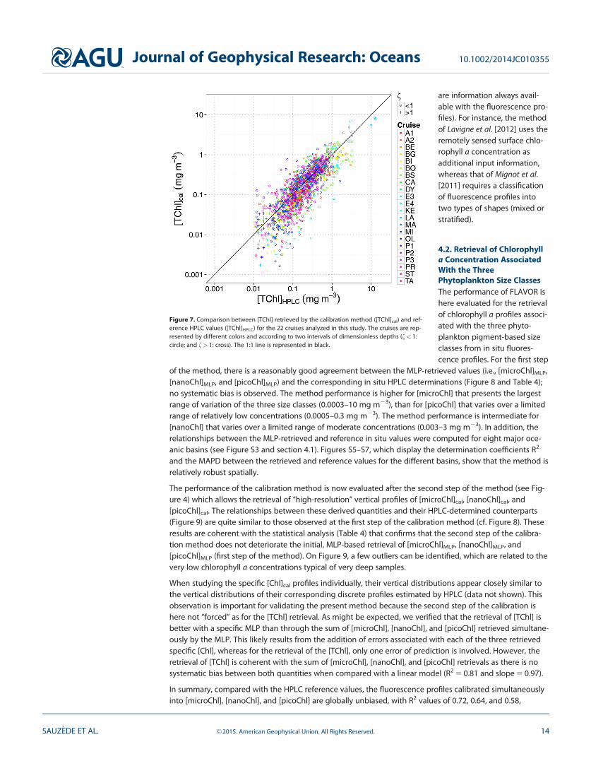
4.1. Retrieval of Chlorophyll a Concentration Associated With the Total Phytoplankton BiomassThe accurate retrieval of [TChl] relies both on the performance of the MLP (first step of the method) and onthe subsequent application of the calibration coefficient a (second step; cf. Figure 4). The scatterplot of the[TChl] values retrieved from the MLP versus those measured by HPLC (Figure 5) reveals that the data are fairlywell distributed around the 1:1 line (see also Table 4 for detailed statistics). This relationship does not showany bias related to the sampling cruise (Figure 5a), therefore suggesting that the proposed method is rela-tively robust both spatially and temporally. To verify this statement, the relationships between the [TChl] val-ues retrieved from the MLP and measured by HPLC were computed for eight major oceanic basins: Antarctic,

Arctic, Mediterranean Sea, Indian, South Pacific, North Pacific,South Atlantic, and North Atlantic Ocean (Figure S3). The deter-mination coefficient, R2, and the MAPD between the retrievedand reference values for the different basins indicate that themethod is robust, with slightly less accurate results for the Arcticbasin and the Indian Ocean which are two areas known for datascarcity (see Figure S4). Nevertheless, Figure 5b shows more scat-ter at low chlorophyll levels which, in general, correspond to thegreatest dimensionless depths f. This observation supports theresults shown in Figure 6 where the determination coefficientsand the MAPD between the [TChl] values derived from the MLPand measured by HPLC were computed for six dimensionlessdepth intervals. The determination coefficient R2 decreases withincreasing f, whereas the corresponding MAPD increases withincreasing f. This supports the idea that the MLP is less robustfor retrieving [TChl] values at large depths. Nevertheless, the rela-tionship between [TChl]MLP and [TChl]HPLC for each of the sixdimensionless depth intervals is significant (pvalue< 0.005). Fur-thermore, it should be noticed that the retrieval of [TChl]MLP is

Figure 5. Comparison between [TChl] retrieved by the MLP ([TChl]MLP) with HPLC reference ([TChl]HPLC). (a) Data identified according to the 22 cruises and (b) data ordered according tothe dimensionless depth f. The HPLC pigment reference values correspond to linear interpolation of the HPLC measurements for the 10 [TChl] restitution depths of the MLP. The 1:1 lineis represented in black in each plot.

Table 4. Comparison of Values Retrieved by theMLP ([Chl]MLP, First Step of Calibration) orThrough the Second Step of Calibration ([Chl]cal)With Concomitant HPLC Reference Values([Chl]HPLC)a

R2 a MAPD (%)

First Step[TChl]MLP 0.74 0.83 32[microChl]MLP 0.73 0.78 44[nanoChl]MLP 0.60 0.69 35[picoChl]MLP 0.57 0.64 44

Second Step[TChl]cal 0.68 0.96 40[microChl]cal 0.72 0.75 46[nanoChl]cal 0.64 0.68 35[picoChl]cal 0.58 0.61 40

aDetermination coefficient (R2) and slope (a)corresponding to linear regression analysesbetween retrieved and reference values. Foreach case, the MAPD (Median Absolute PercentDifference) between retrieved and referencevalues is also indicated.



less critical for deeper layersthan for upper layers wheremost of the phytoplankton bio-mass occurs. The calibrationcoefficient a applied to the insitu fluorescence profile takesinto account only theMLP-predicted values com-prised between surface and Z0

(cf. section 3.3).

The second step of our methodallows the retrieval of cali-brated [TChl] ([TChl]cal) profileswith the same vertical resolu-tion as the initial fluorescenceprofiles. The performance ofthe method is assessedthrough the comparison of[TChl]cal with the correspond-ing in situ HPLC measure-ments, [TChl]HPLC (Figure 7 andTable 4). The relationshipbetween [TChl]cal and[TChl]HPLC appears more scat-tered than the relationshipbetween [TChl]MLP and

[TChl]HPLC (i.e., first step of the method; Figure 5 and Table 4). This might be due, at least partially, to thereintroduction of the signal noise of the in situ measured fluorescence profile into the MLP-retrieved profilethat can be sometimes particularly pronounced. However, compared with the HPLC reference values, thefluorescence profiles calibrated into [TChl] appear globally unbiased.

The impact of the daytime Non-Photochemical Quenching (NPQ) [see, e.g., Cullen and Lewis, 1995], which isresponsible for a reduction in the chlorophyll fluorescence at high irradiance, deserves further considerationin the evaluation of the proposed method. In the first step of FLAVOR, the MLP learning is based on in situmeasurements so that the NPQ is implicitly taken into consideration and thus corrected for a proper restitu-tion of the chlorophyll a concentration (i.e., to a given quenched chlorophyll fluorescence profile is associ-ated an unquenched HPLC-determined chlorophyll a profile). In the second step of FLAVOR, the initialfluorescence profile shape is used to compute the final [TChl]cal (see equation (16)); thus, the potential biasdue to the NPQ is implicitly reintroduced. This is admittedly a weakness of the present method. If densityprofiles are acquired simultaneously to fluorescence profiles, the NPQ could be corrected following themethod of Xing et al. [2012]. This method involves substituting the fluorescence values acquired within themixed layer by the maximum value within this layer. If the concomitant acquisition of density is not avail-able, there is presently no solution to overcome the potential issue of the NPQ.

Finally, the performance of FLAVOR can be compared with that of other methods developed to retrieve thevertical distribution of the total chlorophyll a concentration from fluorescence profiles. The method pro-posed by Lavigne et al. [2012] was evaluated using the long-term time series data sets from the BATS, HOT,and Dyfamed stations. The method developed by Mignot et al. [2011] and the method presented here wereevaluated with data sets representative of the global ocean. Although the performances of these threemethods were assessed on the basis of different data sets, the statistical indices of performance of thesemethods can be compared, at least in an indicative manner. The MAPD is 33%, 31% and 32% for the meth-ods developed by Mignot et al. [2011], Lavigne et al. [2012] and FLAVOR, respectively. In other words, FLA-VOR performs well in comparison to the other methods and presents the additional advantage of beingself-sufficient, i.e., it does not require any other external information or data to retrieve the phytoplanktontotal or class-specific chlorophyll a concentration (except the geo-location and date of acquisition which

Figure 6. Determination coefficient R2 and Median Absolute Percent Difference (MAPD) ofthe linear models between [TChl] retrieved by the MLP ([TChl]MLP) and HPLC reference([TChl]HPLC) values computed for several dimensionless depth intervals. The number ofpoints corresponding to each interval is identified in bracket. The MAPD is presented heredivided by 100 so values range is 0–1.



are information always avail-able with the fluorescence pro-files). For instance, the methodof Lavigne et al. [2012] uses theremotely sensed surface chlo-rophyll a concentration asadditional input information,whereas that of Mignot et al.[2011] requires a classificationof fluorescence profiles intotwo types of shapes (mixed orstratified).

4.2. Retrieval of Chlorophylla Concentration AssociatedWith the ThreePhytoplankton Size ClassesThe performance of FLAVOR ishere evaluated for the retrievalof chlorophyll a profiles associ-ated with the three phyto-plankton pigment-based sizeclasses from in situ fluores-cence profiles. For the first step

of the method, there is a reasonably good agreement between the MLP-retrieved values (i.e., [microChl]MLP,[nanoChl]MLP, and [picoChl]MLP) and the corresponding in situ HPLC determinations (Figure 8 and Table 4);no systematic bias is observed. The method performance is higher for [microChl] that presents the largestrange of variation of the three size classes (0.0003–10 mg m23), than for [picoChl] that varies over a limitedrange of relatively low concentrations (0.0005–0.3 mg m23). The method performance is intermediate for[nanoChl] that varies over a limited range of moderate concentrations (0.003–3 mg m23). In addition, therelationships between the MLP-retrieved and reference in situ values were computed for eight major oce-anic basins (see Figure S3 and section 4.1). Figures S5–S7, which display the determination coefficients R2

and the MAPD between the retrieved and reference values for the different basins, show that the method isrelatively robust spatially.

The performance of the calibration method is now evaluated after the second step of the method (see Fig-ure 4) which allows the retrieval of ‘‘high-resolution’’ vertical profiles of [microChl]cal, [nanoChl]cal, and[picoChl]cal. The relationships between these derived quantities and their HPLC-determined counterparts(Figure 9) are quite similar to those observed at the first step of the calibration method (cf. Figure 8). Theseresults are coherent with the statistical analysis (Table 4) that confirms that the second step of the calibra-tion method does not deteriorate the initial, MLP-based retrieval of [microChl]MLP, [nanoChl]MLP, and[picoChl]MLP (first step of the method). On Figure 9, a few outliers can be identified, which are related to thevery low chlorophyll a concentrations typical of very deep samples.

When studying the specific [Chl]cal profiles individually, their vertical distributions appear closely similar tothe vertical distributions of their corresponding discrete profiles estimated by HPLC (data not shown). Thisobservation is important for validating the present method because the second step of the calibration ishere not ‘‘forced’’ as for the [TChl] retrieval. As might be expected, we verified that the retrieval of [TChl] isbetter with a specific MLP than through the sum of [microChl], [nanoChl], and [picoChl] retrieved simultane-ously by the MLP. This likely results from the addition of errors associated with each of the three retrievedspecific [Chl], whereas for the retrieval of the [TChl], only one error of prediction is involved. However, theretrieval of [TChl] is coherent with the sum of [microChl], [nanoChl], and [picoChl] retrievals as there is nosystematic bias between both quantities when compared with a linear model (R2 5 0.81 and slope 5 0.97).

In summary, compared with the HPLC reference values, the fluorescence profiles calibrated simultaneouslyinto [microChl], [nanoChl], and [picoChl] are globally unbiased, with R2 values of 0.72, 0.64, and 0.58,

Figure 7. Comparison between [TChl] retrieved by the calibration method ([TChl]cal) and ref-erence HPLC values ([TChl]HPLC) for the 22 cruises analyzed in this study. The cruises are rep-resented by different colors and according to two intervals of dimensionless depths (f< 1:circle; and f> 1: cross). The 1:1 line is represented in black.



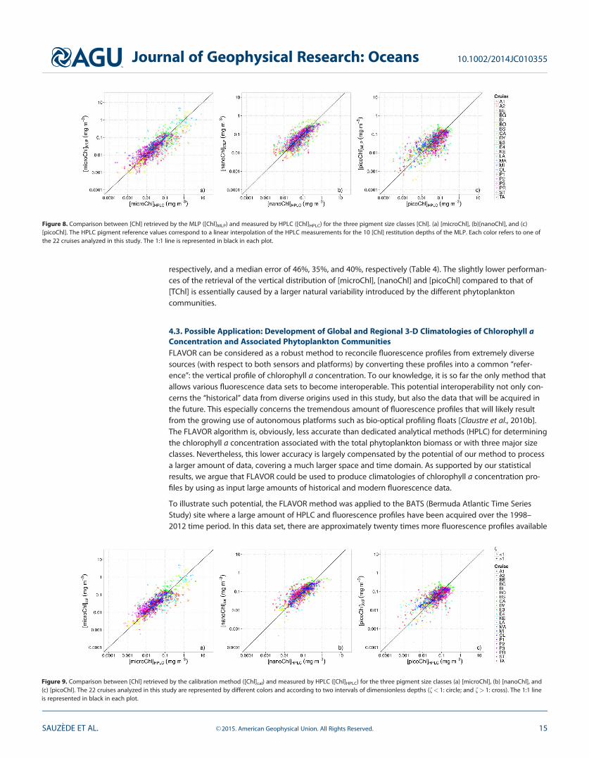
respectively, and a median error of 46%, 35%, and 40%, respectively (Table 4). The slightly lower performan-ces of the retrieval of the vertical distribution of [microChl], [nanoChl] and [picoChl] compared to that of[TChl] is essentially caused by a larger natural variability introduced by the different phytoplanktoncommunities.

4.3. Possible Application: Development of Global and Regional 3-D Climatologies of Chlorophyll aConcentration and Associated Phytoplankton CommunitiesFLAVOR can be considered as a robust method to reconcile fluorescence profiles from extremely diversesources (with respect to both sensors and platforms) by converting these profiles into a common ‘‘refer-ence’’: the vertical profile of chlorophyll a concentration. To our knowledge, it is so far the only method thatallows various fluorescence data sets to become interoperable. This potential interoperability not only con-cerns the ‘‘historical’’ data from diverse origins used in this study, but also the data that will be acquired inthe future. This especially concerns the tremendous amount of fluorescence profiles that will likely resultfrom the growing use of autonomous platforms such as bio-optical profiling floats [Claustre et al., 2010b].The FLAVOR algorithm is, obviously, less accurate than dedicated analytical methods (HPLC) for determiningthe chlorophyll a concentration associated with the total phytoplankton biomass or with three major sizeclasses. Nevertheless, this lower accuracy is largely compensated by the potential of our method to processa larger amount of data, covering a much larger space and time domain. As supported by our statisticalresults, we argue that FLAVOR could be used to produce climatologies of chlorophyll a concentration pro-files by using as input large amounts of historical and modern fluorescence data.

To illustrate such potential, the FLAVOR method was applied to the BATS (Bermuda Atlantic Time SeriesStudy) site where a large amount of HPLC and fluorescence profiles have been acquired over the 1998–2012 time period. In this data set, there are approximately twenty times more fluorescence profiles available

Figure 8. Comparison between [Chl] retrieved by the MLP ([Chl]MLP) and measured by HPLC ([Chl]HPLC) for the three pigment size classes [Chl]. (a) [microChl], (b)[nanoChl], and (c)[picoChl]. The HPLC pigment reference values correspond to a linear interpolation of the HPLC measurements for the 10 [Chl] restitution depths of the MLP. Each color refers to one ofthe 22 cruises analyzed in this study. The 1:1 line is represented in black in each plot.

Figure 9. Comparison between [Chl] retrieved by the calibration method ([Chl]cal) and measured by HPLC ([Chl]HPLC) for the three pigment size classes (a) [microChl], (b) [nanoChl], and(c) [picoChl]. The 22 cruises analyzed in this study are represented by different colors and according to two intervals of dimensionless depths (f< 1: circle; and f> 1: cross). The 1:1 lineis represented in black in each plot.



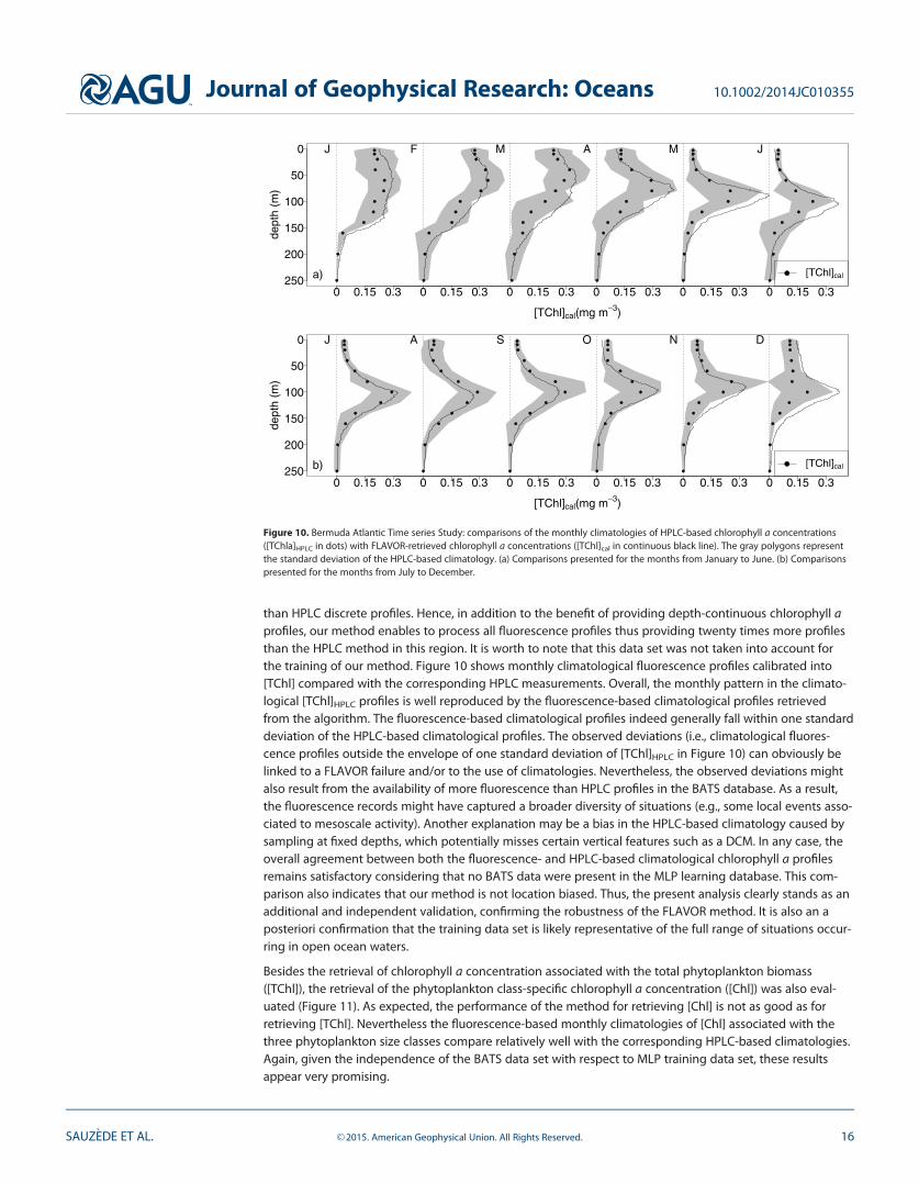
than HPLC discrete profiles. Hence, in addition to the benefit of providing depth-continuous chlorophyll aprofiles, our method enables to process all fluorescence profiles thus providing twenty times more profilesthan the HPLC method in this region. It is worth to note that this data set was not taken into account forthe training of our method. Figure 10 shows monthly climatological fluorescence profiles calibrated into[TChl] compared with the corresponding HPLC measurements. Overall, the monthly pattern in the climato-logical [TChl]HPLC profiles is well reproduced by the fluorescence-based climatological profiles retrievedfrom the algorithm. The fluorescence-based climatological profiles indeed generally fall within one standarddeviation of the HPLC-based climatological profiles. The observed deviations (i.e., climatological fluores-cence profiles outside the envelope of one standard deviation of [TChl]HPLC in Figure 10) can obviously belinked to a FLAVOR failure and/or to the use of climatologies. Nevertheless, the observed deviations mightalso result from the availability of more fluorescence than HPLC profiles in the BATS database. As a result,the fluorescence records might have captured a broader diversity of situations (e.g., some local events asso-ciated to mesoscale activity). Another explanation may be a bias in the HPLC-based climatology caused bysampling at fixed depths, which potentially misses certain vertical features such as a DCM. In any case, theoverall agreement between both the fluorescence- and HPLC-based climatological chlorophyll a profilesremains satisfactory considering that no BATS data were present in the MLP learning database. This com-parison also indicates that our method is not location biased. Thus, the present analysis clearly stands as anadditional and independent validation, confirming the robustness of the FLAVOR method. It is also an aposteriori confirmation that the training data set is likely representative of the full range of situations occur-ring in open ocean waters.

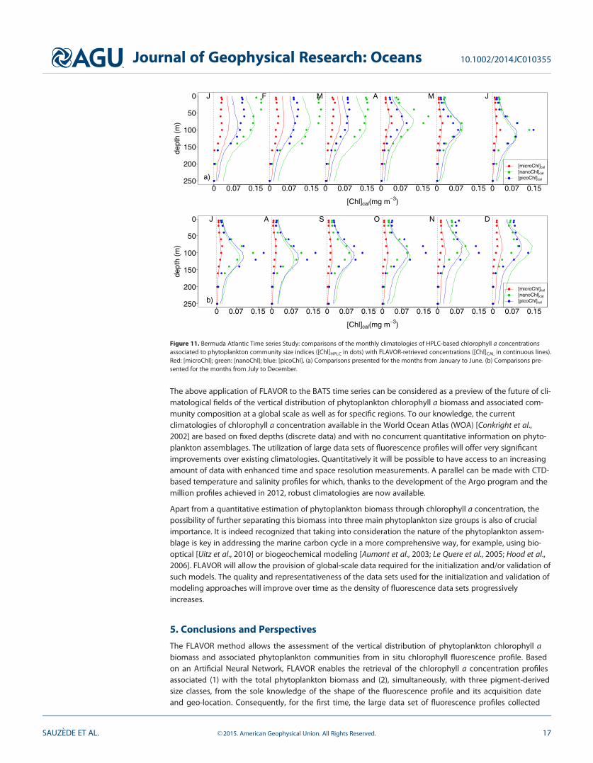
Besides the retrieval of chlorophyll a concentration associated with the total phytoplankton biomass([TChl]), the retrieval of the phytoplankton class-specific chlorophyll a concentration ([Chl]) was also eval-uated (Figure 11). As expected, the performance of the method for retrieving [Chl] is not as good as forretrieving [TChl]. Nevertheless the fluorescence-based monthly climatologies of [Chl] associated with thethree phytoplankton size classes compare relatively well with the corresponding HPLC-based climatologies.Again, given the independence of the BATS data set with respect to MLP training data set, these resultsappear very promising.

Figure 10. Bermuda Atlantic Time series Study: comparisons of the monthly climatologies of HPLC-based chlorophyll a concentrations([TChla]HPLC in dots) with FLAVOR-retrieved chlorophyll a concentrations ([TChl]cal in continuous black line). The gray polygons representthe standard deviation of the HPLC-based climatology. (a) Comparisons presented for the months from January to June. (b) Comparisonspresented for the months from July to December.



The above application of FLAVOR to the BATS time series can be considered as a preview of the future of cli-matological fields of the vertical distribution of phytoplankton chlorophyll a biomass and associated com-munity composition at a global scale as well as for specific regions. To our knowledge, the currentclimatologies of chlorophyll a concentration available in the World Ocean Atlas (WOA) [Conkright et al.,2002] are based on fixed depths (discrete data) and with no concurrent quantitative information on phyto-plankton assemblages. The utilization of large data sets of fluorescence profiles will offer very significantimprovements over existing climatologies. Quantitatively it will be possible to have access to an increasingamount of data with enhanced time and space resolution measurements. A parallel can be made with CTD-based temperature and salinity profiles for which, thanks to the development of the Argo program and themillion profiles achieved in 2012, robust climatologies are now available.

Apart from a quantitative estimation of phytoplankton biomass through chlorophyll a concentration, thepossibility of further separating this biomass into three main phytoplankton size groups is also of crucialimportance. It is indeed recognized that taking into consideration the nature of the phytoplankton assem-blage is key in addressing the marine carbon cycle in a more comprehensive way, for example, using bio-optical [Uitz et al., 2010] or biogeochemical modeling [Aumont et al., 2003; Le Quere et al., 2005; Hood et al.,2006]. FLAVOR will allow the provision of global-scale data required for the initialization and/or validation ofsuch models. The quality and representativeness of the data sets used for the initialization and validation ofmodeling approaches will improve over time as the density of fluorescence data sets progressivelyincreases.

5. Conclusions and Perspectives

The FLAVOR method allows the assessment of the vertical distribution of phytoplankton chlorophyll abiomass and associated phytoplankton communities from in situ chlorophyll fluorescence profile. Basedon an Artificial Neural Network, FLAVOR enables the retrieval of the chlorophyll a concentration profilesassociated (1) with the total phytoplankton biomass and (2), simultaneously, with three pigment-derivedsize classes, from the sole knowledge of the shape of the fluorescence profile and its acquisition dateand geo-location. Consequently, for the first time, the large data set of fluorescence profiles collected

Figure 11. Bermuda Atlantic Time series Study: comparisons of the monthly climatologies of HPLC-based chlorophyll a concentrationsassociated to phytoplankton community size indices ([Chl]HPLC in dots) with FLAVOR-retrieved concentrations ([Chl]CAL in continuous lines).Red: [microChl]; green: [nanoChl]; blue: [picoChl]. (a) Comparisons presented for the months from January to June. (b) Comparisons pre-sented for the months from July to December.



since the 1970s could be harmonized and made interoperable in terms of chlorophyll a concentration.Additionally, it is the first method that allows for the retrieval of the composition of phytoplanktoncommunities from a fluorescence profile. However, it is important to note that to apply the method tofluorescence profiles acquired pre-1991, the assumption has to be made that the relationship betweenthe phytoplankton biomass and the community composition with the fluorescence profile is the sameas for our data set (post 1991).

Validation results have been presented here regarding the retrieval of total and class-specific chlorophyll aconcentration versus in situ HPLC reference measurements. Our method appears to be spatially and tempo-rally robust as the relationships between the retrieved and reference in situ values do not show systematicbias with respect to the different oceanic regions and cruises regardless of the product to be retrieved (Fig-ures 5a and 7–9 and Figures S4–S7). Additionally, because FLAVOR was developed using a data set that isrepresentative of most of the hydrologic and trophic conditions prevailing in the open ocean, it can be con-sidered potentially applicable to any situation occurring in the global open ocean. Nevertheless, it shouldbe emphasized that, although FLAVOR is applicable to situations in which it has not been trained (e.g., theBATS time series; see Figures 10 and 11), its use deserves some caution. FLAVOR is not a method for use ona profile-by-profile basis, where a single fluorescence profile would be injected to retrieve accurate profilesof chlorophyll a concentration for the entire algal biomass and associated size indices. Instead, the methodis intended for use on large data sets for deriving vertical chlorophyll a climatologies from which someregional or temporal trends might possibly be extracted. Such data sets could be exploited to improve theopen ocean climatologies of chlorophyll a concentration.

Hence, thanks to the ongoing and future availability of spatially and temporally well-resolved data sets, itwill become possible to develop 3-D and even 4-D global climatologies of chlorophyll a concentration andassociated community composition in terms of three major phytoplankton size classes. These types of cli-matologies are not only required for the initialization and validation of biogeochemical models but mayalso serve as benchmark for documenting possible changes in phytoplankton biomass and distribution inthe global ocean.

ReferencesAumont, O., E. Maier-Reimer, S. Blain, and P. Monfray (2003), An ecosystem model of the global ocean including Fe, Si, P colimitations,

Global Biogeochem. Cycles, 17(2), 1060, doi:10.1029/2001GB001745.Ben Mustapha, Z., S. Alvain, C. Jamet, H. Loisel, and D. Dessailly (2013), Automatic classification of water-leaving radiance anomalies from

global SeaWiFS imagery: Application to the detection of phytoplankton groups in open ocean waters, Remote Sens. Environ., 146, 97–112, doi:10.1016/j.rse.2013.08.046.

Bishop, C. M. (1995), Neural Networks for Pattern Recognition, 482 pp., Oxford Univ. Press, Oxford, U. K.Brewin, R. J. W., S. Sathyendranath, T. Hirata, S. J. Lavender, R. M. Barciela, and N. J. Hardman-Mountford (2010), A three-component model

of phytoplankton size class for the Atlantic Ocean, Ecol. Modell., 221(11), 1472–1483, doi:10.1016/j.ecolmodel.2010.02.014.Brewin, R. J. W., S. Sathyendranath, P. K. Lange, and G. Tilstone (2014), Comparison of two methods to derive the size-structure of natural

populations of phytoplankton, Deep Sea Res., Part I, 85, 72–79, doi:10.1016/j.dsr.2013.11.007.Bricaud, A., E. Bosc, and D. Antoine (2002), Algal biomass and sea surface temperature in the Mediterranean Basin, Remote Sens. Environ.,

81(2–3), 163–178, doi:10.1016/S0034-4257(01)00335-2.Bricaud, A., C. Mejia, D. Blondeau-Patissier, H. Claustre, M. Crepon, and S. Thiria (2007), Retrieval of pigment concentrations and size struc-

ture of algal populations from their absorption spectra using multilayered perceptrons, Appl. Opt., 46(8), 1251–1260.Buitenhuis, E. T., et al. (2012), Picophytoplankton biomass distribution in the global ocean, Earth Syst. Sci. Data, 4(1), 37–46, doi:10.5194/

essd-4-37-2012.Campbell, J. W. (1995), The lognormal distribution as a model for bio-optical variability in the sea, J. Geophys. Res., 100(C7), 13,231–13,254.Claustre, H. (1994), The trophic status of various oceanic provinces as revealed by phytoplankton pigment signatures, Limnol. Oceanogr.,

39(5), 1206–1210.Claustre, H., and J.-C. Marty (1995), Specific phytoplankton biomasses and their relation to primary production in the tropical North Atlan-

tic, Deep Sea Res., Part I, 42(8), 1475–1493, doi:10.1016/0967-0637(95)00053-9.Claustre, H., P. Kerherv�e, J. C. Marty, L. Prieur, C. Videau, and J.-H. Hecq (1994), Phytoplankton dynamics associated with a geostrophic front:

Ecological and biogeochemical implications, J. Mar. Res., 52(4), 711–742, doi:10.1357/0022240943077000.Claustre, H., A. Morel, M. Babin, C. Cailliau, D. Marie, J.-C. Marty, D. Tailliez, and D. Vaulot (1999), Variability in particle attenuation and chlo-

rophyll fluorescence in the tropical Pacific: Scales, patterns, and biogeochemical implications, J. Geophys. Res., 104(C2), 3401–3422, doi:10.1029/98JC01334.

Claustre, H., F. Fell, K. Oubelkheir, L. Prieur, A. Sciandra, B. Gentili, and M. Babin (2000), Continuous monitoring of surface optical propertiesacross a geostrophic front: Biogeochemical inferences, Limnol. Oceanogr., 45(2), 309–321.

Claustre, H., et al. (2004), An intercomparison of HPLC phytoplankton pigment methods using in situ samples: Application to remote sens-ing and database activities, Mar. Chem., 85(1–2), 41–61, doi:10.1016/j.marchem.2003.09.002.

Claustre, H., M. Babin, D. Merien, J. Ras, L. Prieur, S. Dallot, O. Prasil, H. Dousova, and T. Moutin (2005), Toward a taxon-specific parameteriza-tion of bio-optical models of primary production: A case study in the North Atlantic, J. Geophys. Res., 110, C07S12, doi:10.1029/2004JC002634.

AcknowledgmentsThis paper is a contribution to theRemotely Sensed BiogeochemicalCycles in the Ocean (remOcean)project, funded by the EuropeanResearch Council (grant agreement246777), to the French Bio-Argoproject funded by CNES-TOSCA. TheFrench PROOF and CYBER programsare acknowledged for their support ofmost of the cruises where fluorescenceand HPLC profiles were sampled.Mustapha Ouhssain is acknowledgedfor his contribution to HPLC analysis.The fluorescence and HPLC profilesused in this study can be obtained onrequest at [email protected] [email protected]. The authors wouldlike to thank all the staff of BATSprogram for the periodicmeasurements of oceanographicvariables and for the free distributionof data online (http://bats.bios.edu/).Finally, we are grateful to twoanonymous reviewers for theirvaluable comments and suggestions.



http://bats.bios.edu/

http://dx.doi.org/10.1016/j.rse.2013.08.046

http://dx.doi.org/10.1016/j.ecolmodel.2010.02.014

http://dx.doi.org/10.1016/j.dsr.2013.11.007

http://dx.doi.org/10.1016/S0034-4257(01)00335-2

http://dx.doi.org/10.5194/essd-4-37-2012


http://dx.doi.org/10.1016/0967-0637(95)00053-9

http://dx.doi.org/10.1357/0022240943077000

http://dx.doi.org/10.1029/98JC01334

http://dx.doi.org/10.1016/j.marchem.2003.09.002

http://dx.doi.org/10.1029/2004JC002634

http://dx.doi.org/10.1029/2004JC002634

http://bats.bios.edu/

Claustre, H., et al. (2010a), Bio-optical profiling floats as new observational tools for biogeochemical and ecosystem studies: Potential syn-ergies with ocean color remote sensing, in Proceedings of the OceanObs 09: Sustained Ocean Observations and Information for SocietyConference, vol. 2, edited by J. Hall, D. E. Harrison, and D. Stammer, ESA Publ., Venice, Italy.

Claustre, H., et al. (2010b), Guidelines towards an integrated ocean observation system for ecosystems and biogeochemical cycles, in Pro-ceedings of the OceanObs 09: Sustained Ocean Observations and Information for Society Conference, vol. 1, edited by J. Hall, D. E. Harrison,and D. Stammer, ESA Publ., Venice, Italy.

Conkright, M. E., R. A. Locarnini, H. E. Garcia, T. D. O’Brien, T. P. Boyer, C. Stephens, and J. I. Antonov (2002), World Ocean Atlas 2001: Objec-tive Analyses, Data Statistics, and Figures [CD-ROM], U.S. Dep. of Commer., Natl. Oceanic and Atmos. Admin., Natl. Oceanogr. Data Cent.,Ocean Clim. Lab., Silver Spring, Md.

Crombet, Y., K. Leblanc, B. Qu�eguiner, T. Moutin, P. Rimmelin, J. Ras, H. Claustre, N. Leblond, L. Oriol, and M. Pujo-Pay (2011), Deep siliconmaxima in the stratified oligotrophic Mediterranean Sea, Biogeosciences, 8(2), 459–475, doi:10.5194/bg-8-459-2011.

Cullen, J. J., and M. R. Lewis (1995), Biological processes and optical measurements near the sea surface: Some issues relevant to remotesensing, J. Geophys. Res., 100(C7), 13,255–13,266, doi:10.1029/95JC00454.

Cunningham, A. (1996), Variability of in-vivo chlorophyll fluorescence and its implication for instrument development in bio-optical ocean-ography, Sci. Mar., 60(1), 309–315.

Devred, E., S. Sathyendranath, V. Stuart, and T. Platt (2011), A three component classification of phytoplankton absorption spectra: Applica-tion to ocean-color data, Remote Sens. Environ., 115(9), 2255–2266, doi:10.1016/j.rse.2011.04.025.

D’Ortenzio, F., et al. (2010), White Book on Oceanic autonomous Platforms for Biogeochemical Studies: Instrumentation and Measure(PABIM), version 1.3. [Available at: http://www.obs-vlfr.fr/OAO/file/PABIM white book version1.3.pdf.]

Falkowski, P., D. A. Kiefer, O. S. Division, and L. Angeles (1985), Chlorophyll a fluorescence in phytoplankton: Relationship to photosynthesisand biomass, J. Plankton Res., 7(5), 715–731.

Friedrich, T., and A. Oschlies (2009), Neural network-based estimates of North Atlantic surface pCO 2 from satellite data: A methodologicalstudy, J. Geophys. Res., 114, C03020, doi:10.1029/2007JC004646.

Gordon, H. R., and W. R. McCluney (1975), Estimation of the depth of sunlight penetration in the sea for remote sensing, Appl. Opt., 14(2),413–416, doi:10.1364/AO.14.000413.

Gross, L., S. Thiria, R. Frouin, and B. G. Mitchell (2000), Artificial neural networks for modeling the transfer function between marine reflec-tance and phytoplankton pigment concentration, J. Geophys. Res., 105(C2), 3483–3495, doi:10.1029/1999JC900278.

Hood, R. R., et al. (2006), Pelagic functional group modeling: Progress, challenges and prospects, Deep Sea Res., Part II, 53(5–7), 459–512,doi:10.1016/j.dsr2.2006.01.025.

Hornik, K., M. Stinchcombe, and H. White (1989), Multilayer feedforward networks are universal approximators, Neural Networks, 2, 359–366.

Huot, Y., M. Babin, and F. Bruyant (2013), Photosynthetic parameters in the Beaufort Sea in relation to the phytoplankton community struc-ture, Biogeosciences, 10(5), 3445–3454, doi:10.5194/bg-10-3445-2013.

Jamet, C., H. Loisel, and D. Dessailly (2012), Retrieval of the spectral diffuse attenuation coefficient K d (k) in open and coastal ocean watersusing a neural network inversion, J. Geophys. Res., 117, C10023, doi:10.1029/2012JC008076.

Johnson, K. S., L. J. Coletti, H. W. Jannasch, C. M. Sakamoto, D. D. Swift, and S. C. Riser (2013), Long-term nitrate measurements in the oceanusing the in situ ultraviolet spectrophotometer: Sensor integration into the APEX profiling float, J. Atmos. Oceanic Technol., 30(8), 1854–1866, doi:10.1175/JTECH-D-12-00221.1.

Kiefer, D. A. (1973), Chlorophyll a fluorescence in marine centric diatoms: Responses of chloroplasts to light and nutrient stress, Mar. Biol.,23(1), 39–46, doi:10.1007/BF00394110.

Lavigne, H., F. D’Ortenzio, H. Claustre, and A. Poteau (2012), Towards a merged satellite and in situ fluorescence ocean chlorophyll product,Biogeosciences, 9(6), 2111–2125, doi:10.5194/bg-9-2111-2012.

Le Quere, C., et al. (2005), Ecosystem dynamics based on plankton functional types for global ocean biogeochemistry models, GlobalChange Biol, 11, 2016–2040.

Leblanc, K., et al. (2012), A global diatom database—Abundance, biovolume and biomass in the world ocean, Earth Syst. Sci. Data, 4, 149–165.

Lek, S., and J. F. Gu�egan (1999), Artificial neural networks as a tool in ecological modelling, an introduction, Ecol. Modell., 120(2–3), 65–73,doi:10.1016/S0304-3800(99)00092-7.

Lorenzen, C. J. (1966), A method for the continuous measurement of in vivo chlorophyll concentration, Deep Sea Res. Oceanogr. Abstr.,13(2), 223–227, doi:10.1016/0011-7471(66)91102-8.

Marty, J.-C., J. Chiav�erini, M.-D. Pizay, and B. Avril (2002), Seasonal and interannual dynamics of nutrients and phytoplankton pigments inthe western Mediterranean Sea at the DYFAMED time-series station (1991–1999), Deep Sea Res., Part II, 49(11), 1965–1985, doi:10.1016/S0967-0645(02)00022-X.

Marzban, C. (2009), Basic statistics and basic AI: Neural networks, in Artificial Intelligence Methods in the Environmental Sciences, edited byS. E. Haupt, A. Pasini, and C. Marzban, pp. 15–47, Springer, Netherlands.

McClain, C. R. (2009), A decade of satellite ocean color observations, Annu. Rev. Mar. Sci., 1, 19–42, doi:10.1146/annurev.marine.010908.163650.

Mignot, A., H. Claustre, F. D’Ortenzio, X. Xing, A. Poteau, and J. Ras (2011), From the shape of the vertical profile of in vivo fluorescence tochlorophyll-a concentration, Biogeosciences, 8(2), 3697–3737, doi:10.5194/bgd-8-3697-2011.

Morel, A., and J.-F. Berthon (1989), Surface pigments, algal biomass profiles, and potential production of the euphotic layer: Relationshipsreinvestigated in view of remote-sensing applications, Limnol. Oceanogr., 34(8), 1545–1562.

Morel, A., and S. Maritorena (2001), Bio-optical properties of oceanic waters: A reappraisal, J. Geophys. Res., 106(C4), 7163–7180, doi:10.1029/2000JC000319.

Morel, A., B. Gentili, M. Chami, and J. Ras (2006), Bio-optical properties of high chlorophyll Case 1 waters and of yellow-substance-dominated Case 2 waters, Deep Sea Res., Part I, 53(9), 1439–1459, doi:10.1016/j.dsr.2006.07.007.

Palacz, A. P., M. A. St. John, R. J. W. Brewin, T. Hirata, and W. W. Gregg (2013), Distribution of phytoplankton functional types in high-nitrate,low-chlorophyll waters in a new diagnostic ecological indicator model, Biogeosciences, 10(11), 7553–7574, doi:10.5194/bg-10-7553-2013.

Peloquin, J., et al. (2013), The MAREDAT global database of high performance liquid chromatography marine pigment measurements,Earth Syst. Sci. Data, 5(1), 109–123, doi:10.5194/essd-5-109-2013.

Raitsos, D. E., S. J. Lavender, C. D. Maravelias, J. Haralabous, A. J. Richardson, and P. C. Reid (2008), Identifying four phytoplankton functionaltypes from space: An ecological approach, Limnol. Oceanogr., 53(2), 605–613.



http://dx.doi.org/10.5194/bg-8-459-2011

http://dx.doi.org/10.1029/95JC00454


http://www.obs-vlfr.fr/OAO/file/PABIM white book version1.3.pdf

http://dx.doi.org/10.1029/2007JC004646

http://dx.doi.org/10.1364/AO.14.000413

http://dx.doi.org/10.1029/1999JC900278

http://dx.doi.org/10.1016/j.dsr2.2006.01.025

http://dx.doi.org/10.5194/bg-10-3445-2013

http://dx.doi.org/10.1029/2012JC008076

http://dx.doi.org/10.1175/JTECH-D-12-00221.1

http://dx.doi.org/10.1007/BF00394110

http://dx.doi.org/10.5194/bg-9-2111-2012

http://dx.doi.org/10.1016/S0304-3800(99)00092-7

http://dx.doi.org/10.1016/0011-7471(66)91102-8

http://dx.doi.org/10.1016/S0967-0645(02)00022-X

http://dx.doi.org/10.1016/S0967-0645(02)00022-X

http://dx.doi.org/10.1146/annurev.marine.010908.163650

http://dx.doi.org/10.1146/annurev.marine.010908.163650

http://dx.doi.org/10.5194/bgd-8-3697-2011

http://dx.doi.org/10.1029/2000JC000319


http://dx.doi.org/10.5194/bg-10-7553-2013

http://dx.doi.org/10.5194/bg-10-7553-2013


Ras, J., H. Claustre, and J. Uitz (2008), Spatial variability of phytoplankton pigment distributions in the Subtropical South Pacific Ocean:Comparison between in situ and predicted data, Biogeosciences, 5(2), 353–369.

Siegel, D. A., et al. (2013), Regional to global assessments of phytoplankton dynamics from the SeaWiFS mission, Remote Sens. Environ.,135, 77–91, doi:10.1016/j.rse.2013.03.025.

Telszewski, M., et al. (2009), Estimating the monthly pCO2 distribution in the north Atlantic using a self-organizing neural network, Biogeo-sciences, 6, 1405–1421.

Uitz, J., H. Claustre, A. Morel, and S. B. Hooker (2006), Vertical distribution of phytoplankton communities in open ocean: An assessmentbased on surface chlorophyll, J. Geophys. Res., 111, C08005, doi:10.1029/2005JC003207.

Uitz, J., H. Claustre, F. B. Griffiths, J. Ras, N. Garcia, and V. Sandroni (2009), A phytoplankton class-specific primary production model appliedto the Kerguelen Islands region (Southern Ocean), Deep Sea Res., Part I, 56(4), 541–560, doi:10.1016/j.dsr.2008.11.006.

Uitz, J., H. Claustre, B. Gentili, and D. Stramski (2010), Phytoplankton class-specific primary production in the world’s oceans: Seasonal andinterannual variability from satellite observations, Global Biogeochem. Cycles, 24, GB3016, doi:10.1029/2009GB003680.

Vidussi, F., H. Claustre, J. Bustillos-Guzm�an, C. Cailliau, and J.-C. Marty (1996), Determination of chlorophylls and carotenoids of marine phy-toplankton: Separation of chlorophyll a from divinylchlorophyll a and zeaxanthin from lutein, J. Plankton Res., 18(12), 2377–2382, doi:10.1093/plankt/18.12.2377.

Vidussi, F., H. Claustre, B. B. Manca, A. Luchetta, and J.-C. Marty (2001), Phytoplankton pigment distribution in relation to upper thermoclinecirculation in the eastern Mediterranean Sea during winter, J. Geophys. Res., 106(C9), 19,939–19,956, doi:10.1029/1999JC000308.

Xing, X., H. Claustre, S. Blain, F. D’Ortenzio, D. Antoine, J. Ras, and C. Guinet (2012), Quenching correction for in vivo chlorophyll fluores-cence acquired by autonomous platforms: A case study with instrumented elephant seals in the Kerguelen region (Southern Ocean),Limnol. Oceanogr. Methods, 10, 483–495, doi:10.4319/lom.2012.10.483.




http://dx.doi.org/10.1029/2005JC003207


http://dx.doi.org/10.1029/2009GB003680

http://dx.doi.org/10.1093/plankt/18.12.2377

http://dx.doi.org/10.1029/1999JC000308

http://dx.doi.org/10.4319/lom.2012.10.483

retrieving the vertical distribution of chlorophyll a ... · readme figure s1 figure s2 figure s3...

Documents