resource-constrained project scheduling for timely project completion with stochastic activity...

Resource-Constrained Project Scheduling for TimelyProject Completion with Stochastic Activity Durations

Francisco BallestınDepartment of Statistics and Operations Research, Universidad Publica de Navarra, Campus de Arrosadıa, 31006 Pamplona, Spain,

[email protected]

Roel LeusDepartment of Decision Sciences and Information Management, Katholieke Universiteit Leuven, 3000 Leuven,

Belgium, [email protected]

We investigate resource-constrained project scheduling with stochastic activity durations. Various objectivefunctions related to timely project completion are examined, as well as the correlation between these

objectives. We develop a GRASP-heuristic to produce high-quality solutions, using so-called descriptive sam-pling. The algorithm outperforms existing algorithms for expected-makespan minimization. The distribution ofthe possible makespan realizations for a given scheduling policy is also studied.

Key words: project scheduling; resource constraints; uncertainty; stochastic activity durations; GRASPHistory: Received: July 2007; Accepted: September 2008 by Panos Kouvelis; after 2 revisions.

1. IntroductionThe larger part of the scientific literature on resource-constrained project scheduling focuses on the mini-mization of project duration in a deterministic setting.The goal of the resource-constrained project schedul-ing problem (RCPSP) is to minimize the duration ofa project subject to finish–start precedence constraintsand renewable resource constraints. It is shown inBlazewicz et al. (1983) that the RCPSP, as a job-shopgeneralization, is NP-hard in the strong sense. A largenumber of exact and heuristic procedures have beenproposed to construct workable baseline schedulesthat solve this deterministic RCPSP; see Demeuleme-ester and Herroelen (2002), Kolisch and Padman(2001) and Neumann et al. (2002) for recent over-views and Herroelen (2005) for a discussion on thelink between theory and practice.

During project execution, however, project activitiesare often subject to considerable uncertainty, whichderives from many different possible sources: activi-ties may take more or less time than originallyestimated, resources may become unavailable, mate-rials may arrive behind schedule, workers may beabsent, etc. In this article, we examine the case wherethis uncertainty is important enough to be incor-porated into the planning phase. The sources ofvariability in processing times are manifold; never-theless, the main scheduling objectives are mostlyfunctions of the activities’ start (or end) times, theproject makespan being the single most-studied ob-

jective, in addition to other ones such as weightedearliness-tardiness and net present value of theproject. This justifies a restriction to the study of un-certainty in processing times only, although thisvariability may be generated by many causes. Thestochastic RCPSP (SRCPSP) is the stochastic equiva-lent of the RCPSP, where activity durations are notknown in advance but are represented as randomvariables. The probability distributions can either beobjective (a risk situation) or result from subjectivejudgment (in the case of decision-theoretic uncertaintyor even ignorance).

The SRCPSP usually aims at minimizing theexpected makespan over a limited set of possibledecisions to be made during project execution. As co-herently described by Stork (2001), an important newaspect comes into play when we move from the de-terministic to the stochastic case: what is a solutionto an SRCPSP-instance? A deterministic scheduledoes not necessarily contain enough information tomake decisions during project execution. Hence, foreach possible event occurring during project execu-tion, a solution should define an appropriate action,typically the start of new activities. To make suchdecisions, one may want to exploit the informationgiven by the current state of the project. In line withIgelmund and Radermacher (1983), among others, wecall such a solution a (scheduling) policy.

A vast amount of literature exists on the so-called(generalized) PERT-problem, where no resource con-straints are taken into consideration. These studies are

459

PRODUCTION AND OPERATIONS MANAGEMENTVol. 18, No. 4, July–August 2009, pp. 459–474ISSN 1059-1478|EISSN 1937-5956|09|1804|0459

POMSDOI 10.3401/poms.1080.01023

r 2009 Production and Operations Management Society

I:/Bwus/Poms/1023/[email protected]

I:/Bwus/Poms/1023/[email protected]

usually concerned with the computation of certaincharacteristics of the project makespan (earliestproject completion), mainly with exact computation,approximation and bounding of the distribution func-tion and the expected value. Note that in this case, noreal scheduling effort is required: all activities can bestarted when their predecessors are completed. For areview of research up until 1987, we refer to Adlakhaand Kulkarni (1989). A recent computational studyon bounding the makespan distribution, in which themost promising algorithms are compared, was con-ducted by Ludwig et al. (2001).

Research into SRCPSP, however, has remainedlimited to date, with few computational publicationsaddressing this problem: Igelmund and Radermacher(1983) and Stork (2001) report on experiments withbranch-and-bound algorithms, while Golenko-Ginzburgand Gonik (1997) and Tsai and Gemmill (1998)develop greedy and local-search heuristics. Time/resource trade-offs with stochastic activity durations,in which resource allocation influences the mean and/or the variance of the durations, are investigated inGerchak (2000), Gutjahr et al. (2000) and Wollmer(1985).

The contributions of this article are fivefold: (1) weexamine multiple possible objective functions for pro-ject scheduling with stochastic activity durations; (2)using computational experiments, we show that thesedifferent objective functions are closely connected andthat, for most practical purposes, it may suffice tofocus on minimizing the expected makespan; (3) wedevelop a GRASP-heuristic that produces high-qual-ity solutions, outperforming existing algorithms forexpected-makespan minimization; (4) the variance-re-duction technique of descriptive sampling is appliedand its benefits assessed; and (5) the distribution ofmakespan realizations for a given scheduling policy isstudied.

The remainder of this article is organized as follows.Definitions and a detailed problem statement are pro-vided in Section 2, followed by a discussion of thecomputational setup (Section 3). Section 4 presents thebasic ingredients of our GRASP-algorithm. Our maincomputational results for the expected-makespanobjective can be found in Section 5; the relationshipbetween the expected makespan and some otherobjective functions is treated in Section 6. The dis-tribution of the makespan realizations is the subject ofSection 7. Finally, a summary is given in Section 8.

2. Definitions and Problem StatementThis section contains a number of definitions (Section2.1), a discussion of scheduling policies (Section 2.2),and a statement of the problems to be solved (Sec-tion 2.3).

2.1. DefinitionsA project consists of a set of activities N 5 f0, 1, . . ., ng,which are to be processed without interruption on anumber K of renewable resource types with availabil-ity ak, k 5 1, . . ., K; each activity i requires rik 2 N unitsof resource type k. The duration Di of activity i is arandom variable (r.v.); the vector (D0, D1, . . ., Dn) isdenoted by D. The set A is a (strict) partial order onN, i.e., an irreflexive and transitive binary relation,which represents technological precedence con-straints. (Dummy) activities 0 and n represent startand end of the project, respectively, and are the(unique) least and greatest element of the partiallyordered set (N, A). Activities 0 and n have zero re-source usage and Pr[Di 5 0] 5 1 for i 5 0, n; for theremaining activities iANf0, ng we assume thatPr[Dio0] 5 0 (Pr[e] represents the probability of evente). We associate the directed acyclic graph G(N, A)with the partially ordered set (N, A).

We use lowercase vector d 5 (d0, d1, . . ., dn) to repre-sent one particular realization (or sample, or scenario)of D. Alternatively, when each duration Di is a con-stant, which is the case in the (deterministic) RCPSP,we use the same notation d. A solution for the RCPSPis a schedule s, i.e., a vector of starting times(s0, s1, . . ., sn) with si � 0 for all iAN, that is bothtime-feasible and resource-feasible. Schedule s iscalled time-feasible if si1di � sj for all (i, j)AA; s is saidto be resource-feasible if, at any time t and for eachresource type k, it holds that

Pi2Aðs;tÞ rik � ak, where

the active set A(s, t) 5 fiAN|si � tosi1dig containsthe activities in N\f0, ng that are in progress at time t.The objective function of the RCPSP is the projectmakespan sn (which is to be minimized).

2.2. Scheduling PoliciesThe execution of a project in the context of theSRCPSP can best be seen as a dynamic decisionprocess. A solution, then, is a policy P, which definesactions at decision times. Decision times are typicallyt 5 0 (the start of the project) and the completion timesof activities. An action can entail the start of a set ofactivities that is precedence and resource feasible. Aschedule is thus gradually constructed through time.A decision at time t can only use information availablebefore or at time t; this requirement is often referredto as the non-anticipativity constraint. As soon asall activities are completed, activity durations areknown, yielding a realization d of D. Consequently,every policy P may alternatively be interpreted (cf.Igelmund and Radermacher 1983; Stork 2001) as afunction Rnþ1

� 7!Rnþ1� that maps given samples d of

activity durations to vectors sðd;PÞ 2 Rnþ1 of feasibleactivity starting times (schedules); if no misinterpre-tation is possible, we usually omit the identification ofthe policy and write s(d). For a given scenario d and

Ballestın and Leus: Resource-Constrained Project Scheduling for Timely Project Completion460 Production and Operations Management 18(4), pp. 459–474, r 2009 Production and Operations Management Society

policy P, sn(d;P) denotes the makespan of the sched-ule. The most-studied objective for the SRCPSP is theselection of a policy P� within a specific class thatminimizes E[sn(D;P)], with E[ � ] the expectation op-erator with respect to D.

A well-known class of scheduling policies is theclass of priority policies, which order all activities ac-cording to a priority list and, at every decision pointt, start as many activities as possible in the orderdictated by the list, which is in line with the parallelschedule generation scheme (parallel SGS) (seeKolisch and Hartmann 1999). These list-schedulingpolicies have a number of drawbacks. First of all,priority policies cannot guarantee an optimal sched-ule. Moreover, changes in activity duration may leadto so-called Graham anomalies (Graham 1966), suchas increasing project duration due to decreasingactivity duration. Stork (2001) describes how, if weinterpret a policy as a function, these anomalies leadus to conclude that priority policies are neither mono-tone nor continuous.

Several other classes of policies have been exam-ined by Stork (2001), most of which exhibit severecomputational limitations; he concludes that, forlarger instances, the only remaining alternative is touse the class of so-called activity-based policies,which is also the class that will be studied in thispaper (Stork uses the term ‘‘job-based (priority)policies’’). An activity-based policy P(L) is alsorepresented by a priority list L of the activities and,for a given sample d, computes starting times bystarting each activity in the order imposed by Las early as possible, with the side constraintthat si(d) � sj(d) if i �L j. Elimination of this side con-straint would yield a simple priority policy thatsuffers from the Graham anomalies, but the ‘‘activ-ity-based’’ point of view, rather than the greedy‘‘resource-based’’ one, eliminates this problem. Sincethese activity-based policies perform activity incre-mentation rather than time incrementation, they arealternatively referred to as ‘‘(stochastic) serial SGS’’(Ballestın 2007).

We provide a small example to illustrate the differ-ence between activity-based policies and simplepriority policies. Consider a project with activity setN 5 f0, . . ., 4g containing three non-dummy activities1, 2 and 3; for the precedence constraints we haveA(f1, 2, 3g) 5 f(1, 2)g, with A(E) the edges of the sub-graph of G(N, A) that is induced by E � N. There isone resource type (K 5 1), with ri1 51 for i 5 1, 2, 3,and availability a1 5 2. The list L corresponding with0 �L 1 �L 2 �L 3 �L 4 can be used to define either apriority policy or an activity-based policy. The prioritypolicy will start both activity 1 and 3 at time 0, whilethe activity-based policy will not start activity 3 earlierthan the starting time of activity 2 because 2 �L 3.

2.3. Problem StatementThe literature on project management abounds withmotivations for reducing project lead times, includingvarious first-mover advantages in new-product de-velopment (see, for instance, Smith and Reinertsen1991), advantages during the bidding process(Kerzner 1998; Newbold 1998; Xie et al. 2006), andincentive contracts that contain a penalty for delayedcompletion or a bonus for early delivery (Bayiz andCorbett 2005). This justifies our focus on timely projectcompletion by using some characterization of themakespan (which is a stochastic variable) as anobjective function. We elaborate on this choice in theparagraphs below.

2.3.1. Individual Projects. French (1988) describesfour criteria for decision making under uncertainty.For a minimization problem, these amount to (1)minimax (minimize the worst possible makespanrealization), (2) minimin (minimize the bestpossible outcome, which is an optimistic approach,as opposed to the pessimistic minimax), (3) minimaxregret (minimize the largest possible difference inmakespan between the policy to be selected and theoptimal makespan for a given realization), and (4)minimize the objective in expectation. Scheduling withobjectives (1) and (3) is studied in Kouvelis and Yu(1997); we do not adopt these objectives because(a) one normally needs discrete scenarios instead ofcontinuous distributions, and (b) the optimizationproblem with constant durations should be easy(solvable in polynomial time) in order to producecomputational results for average-size instances(in the case of Kouvelis and Yu: single-machinescheduling with total-flow-time objective and two-machine flow-shop with makespan objective). Since apractical decision maker is usually risk-averse, wealso do not investigate objective (2).

In conclusion, when a project is to be executed inisolation (e.g., for internal clients), the expectedmakespan (subsequently also called the expectationobjective) is the most logical objective of the forego-ing. Actually, it is well known that the expectationcriterion is most appropriate for a risk-neutraldecision maker. In order to represent possible riskaverseness, we opt for constraints of the formPr[sn(D) � d] � p, for given probability p and dead-line d, rather than for utility functions with theirinherent difficulty of estimation. This reflects theundesirability of exceptionally high makespan real-izations and is comparable with downside-risk orValue-at-Risk (VaR) constraints in Finance (Ang et al.2006; Jorion 2000). Likewise, Schuyler (2001) alsoadvocates conservatism when associating largepotential gains and losses with individual decisions.Henceforth, in line with Portougal and Trietsch

Ballestın and Leus: Resource-Constrained Project Scheduling for Timely Project CompletionProduction and Operations Management 18(4), pp. 459–474, r 2009 Production and Operations Management Society 461

(1998), max Pr[sn � d] is referred to as the service-levelobjective due to its similarity with inventory man-agement (see, for instance, Silver et al. 1998). Forthe benefit of risk averseness, a lower bound may beimposed on the service level. In the remainder of thistext, we use the term statistic to refer to any functionof sn. Obviously, a decision maker may be interestedin possible trade-offs between different statistics;the correlation between statistics will be studied inSection 6.

A second way to account for risk averseness is toinvestigate the trade-off between the expected make-span E[sn(D)] and the makespan variance var[sn(D)].This is in line with Portougal and Trietsch (1998),who suggest that ‘‘variance reduction should beintroduced explicitly in the objective, while retainingthe expected completion time as well’’. Similarly,Elmaghraby et al. (1999) also distinguish both meanand variance of the project duration as the two primeperformance measures of concern. Gutierrez andPaul (2001) examine the impact of variability in ac-tivity duration on mean project duration, while Choand Yum (1997) focus on the sensitivity of makespanvariability. Finally, knowledge of the entire distribu-tion function of makespan realizations for a givenpolicy is obviously also highly informative to thedecision maker; we investigate this in a separatesection (Section 7).

2.3.2. External Clients. The foregoing discussionlooked into the execution of a project in isolation.When a project deadline has been negotiated withexternal clients beforehand, however, it may be moreuseful to adapt the scheduling objective function inorder to reflect existing penalty structures (we do notfocus on bonuses for early completion), which takethe form either of a fixed charge, so that the objectivefunction becomes max Pr[sn � d] for a given deadlined, or of a fixed charge per unit-time overrun, leadingto min E[max{0; sn–d}] (the tardiness objective). Werefer to Gutjahr et al. (2000) for a model that uses moregeneral loss functions in a slightly different context.

3. Computational Setup

3.1. General SettingThe analyses in the next sections are based oncomputational experiments using randomly gener-ated datasets. The coding was performed in C usingthe Microsoft Visual C11 6.0 programming environ-ment, and the experiments were run on a SamsungX15 Plus portable computer with Pentium M proces-sor with 1,400 MHz clock speed and 512 MB RAM,equipped with Windows XP. Our tests were per-formed on instances from the benchmark libraryPSPLIB,1 which contains instances of different size

and with different characteristics of the deterministicRCPSP, and which were generated by the problemgenerator ProGen (Kolisch and Sprecher 1996); thenumber of resource types K � 4. We only use thedataset containing 600 instances with 120 activities(commonly named ‘‘j120’’). The deterministic dura-tion d�i for each activity i 6¼0, n is an integer randomlychosen from f1, 2, . . ., 10g.

We generate the probability distributions of the sto-chastic activity processing times Di (which are notcreated by the ProGen instance generator) in line withStork (2001): we take the given deterministic process-ing time d�i of each activity as expectation andwe construct Uniform, Exponential and Betadistributions. More specifically, we examine fivedistributions: a (continuous) Uniform distribution ond�i �

ffiffiffiffiffid�i

p; d�i þ

ffiffiffiffiffid�i

p� �(subsequently referred to as case

‘‘U1’’); (continuous) Uniform on ½0; 2d�i (‘‘U2’’);Exponential with expectation d�i (‘‘Exp’’); Betadistribution with support ½d�i =2; 2d�i and variance 5

d�i =3 (‘‘B1’’); and Beta with support ½d�i =2; 2d�i andvariance 5 d�2i =3 (‘‘B2’’). These five distributions havevariances of d�i =3; d�2i =3; d�2i ; d�i =3, and d�2i =3, respec-tively. The distributions have been created so that U1and B1, on the one hand, and U2 and B2, on the otherhand, share the same variance.

3.2. Evaluation of the StatisticsExact evaluation of the statistics under consideration(expectation, variance, etc.) would be overly time-consuming (for the expected makespan, for instance,this amounts to the PERT-problem, which is wellknown to constitute a formidable computationalchallenge, see Hagstrom 1988), which is why weapproximate these values by means of simulation.Similar decisions in the context of scheduling underuncertainty have been made by Ballestın (2007), Leusand Herroelen (2004), Mohring and Radermacher(1989) and Stork (2001), among others. A solution inthis article is an activity-based policy P(L), which isrepresented by an activity list L. An approximationof any statistic g(L) associated with P(L) is based onsampling a number of realizations from D; the num-ber of replications is a parameter. Stork (2001), forinstance, states that, for the expected makespan, 200samples turn out to provide a reasonable trade-offbetween precision and computational effort.

For our computational experiments, we examinedthe standard deviation of the percentage deviation ofsimulated versus ‘‘true’’ makespan, the latter obtainedfrom a high number (25,000) of runs over the dataset.For a justification of the standard deviation as anaccuracy measure and for a discussion of the con-vergence of the estimate towards the true value as thenumber of samples increases, see Kleywegt et al. (2001).Leus and Herroelen (2004) note that the number of


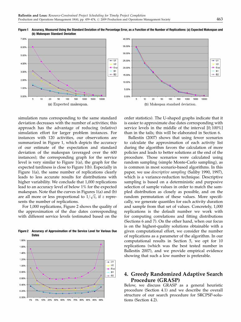
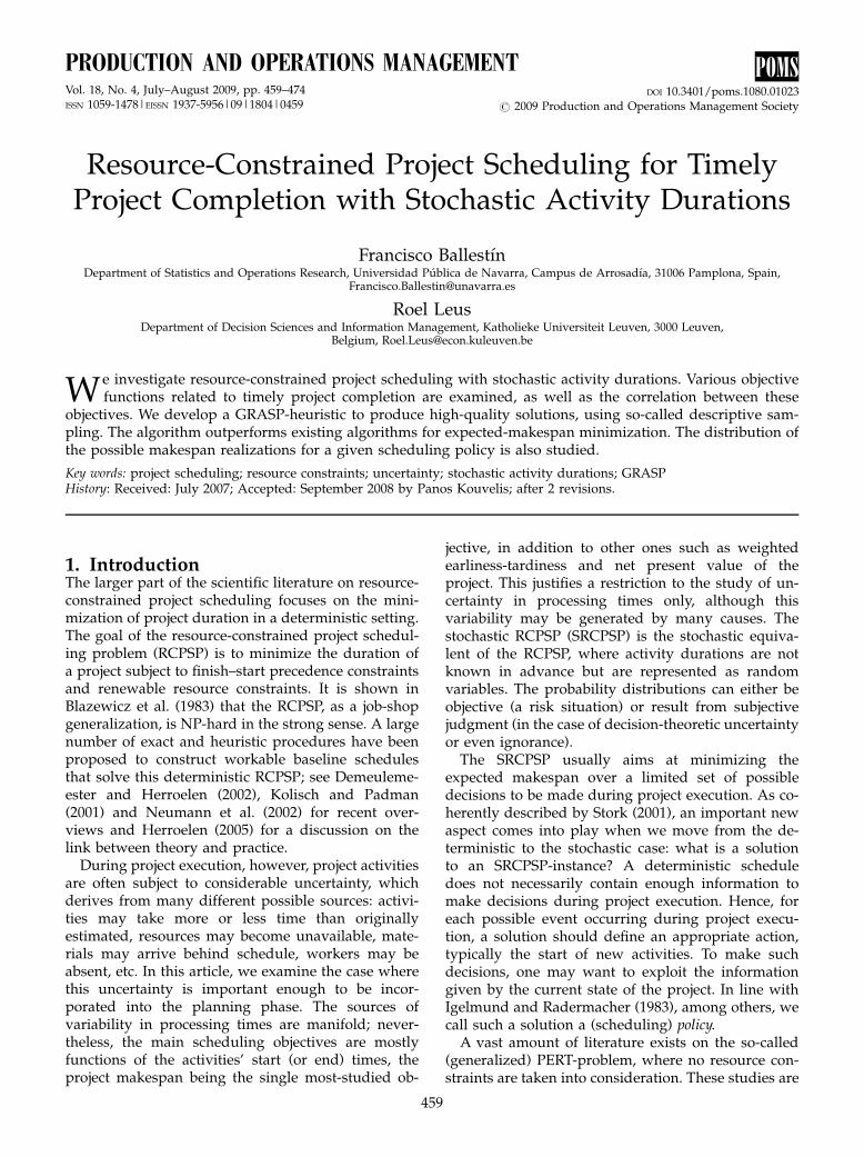
simulation runs corresponding to the same standarddeviation decreases with the number of activities; thisapproach has the advantage of reducing (relative)simulation effort for larger problem instances. Forinstances with 120 activities, our observations aresummarized in Figure 1, which depicts the accuracyof our estimate of the expectation and standarddeviation of the makespan (averaged over the 600instances); the corresponding graph for the servicelevel is very similar to Figure 1(a), the graph for theexpected tardiness is close to Figure 1(b). Especially inFigure 1(a), the same number of replications clearlyleads to less accurate results for distributions withhigher variability. We conclude that 1,000 replicationslead to an accuracy level of below 1% for the expectedmakespan. Note that the curves in Figures 1(a) and (b)are all more or less proportional to 1=

ffiffiffizp

, if z repre-sents the number of replications.

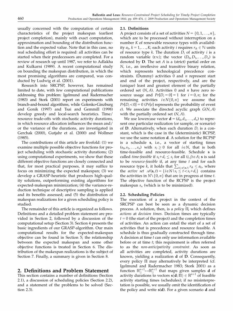
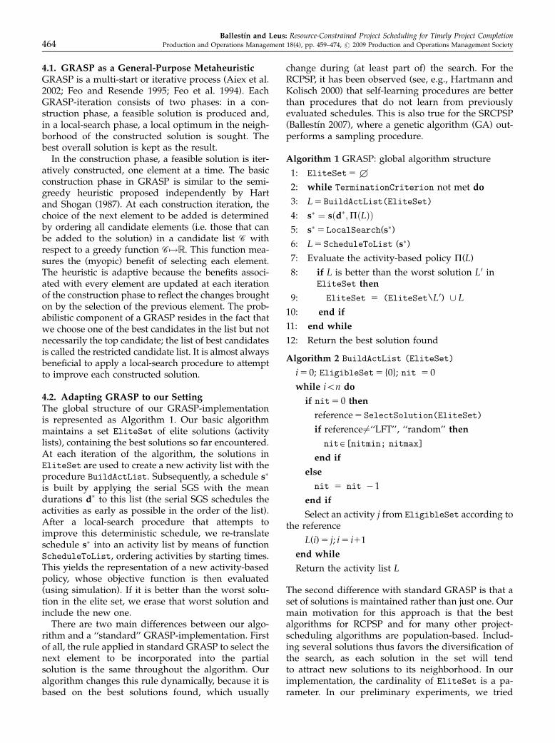
For 1,000 replications, Figure 2 shows the quality ofthe approximation of the due dates correspondingwith different service levels (estimated based on the

order statistics). The U-shaped graphs indicate that itis easier to approximate due dates corresponding withservice levels in the middle of the interval [0; 100%]than in the tails; this will be elaborated in Section 6.

Ballestın (2007) shows that using fewer scenariosto calculate the approximation of each activity listduring the algorithm favors the calculation of morepolicies and leads to better solutions at the end of theprocedure. Those scenarios were calculated usingrandom sampling (simple Monte-Carlo sampling), asis common in most scenario-based algorithms. In thispaper, we use descriptive sampling (Saliby 1990, 1997),which is a variance-reduction technique. Descriptivesampling is based on a deterministic and purposiveselection of sample values in order to match the sam-pled distribution as closely as possible, and on therandom permutation of these values. More specifi-cally, we generate quantiles for each activity durationand sample from that set of values. Concretely, 1,000replications is the default number we work withfor computing correlations and fitting distributions(Sections 6 and 7). On the other hand, when our focusis on the highest-quality solutions obtainable with agiven computational effort, we consider the numberof replications as a parameter of the algorithm. In ourcomputational results in Section 5, we opt for 10replications (which was the best tested number inBallestın 2007), and we provide empirical evidenceshowing that such a low number is preferable.

4. Greedy Randomized Adaptive SearchProcedure (GRASP)

Below, we discuss GRASP as a general heuristicprocedure (Section 4.1) and we describe the overallstructure of our search procedure for SRCPSP-solu-tions (Section 4.2).

Figure 1 Accuracy, Measured Using the Standard Deviation of the Percentage Error, as a Function of the Number of Replications: (a) Expected Makespan and(b) Makespan Standard Deviation

Figure 2 Accuracy of Approximation of the Service Level for Various DueDates


4.1. GRASP as a General-Purpose MetaheuristicGRASP is a multi-start or iterative process (Aiex et al.2002; Feo and Resende 1995; Feo et al. 1994). EachGRASP-iteration consists of two phases: in a con-struction phase, a feasible solution is produced and,in a local-search phase, a local optimum in the neigh-borhood of the constructed solution is sought. Thebest overall solution is kept as the result.

In the construction phase, a feasible solution is iter-atively constructed, one element at a time. The basicconstruction phase in GRASP is similar to the semi-greedy heuristic proposed independently by Hartand Shogan (1987). At each construction iteration, thechoice of the next element to be added is determinedby ordering all candidate elements (i.e. those that canbe added to the solution) in a candidate list C withrespect to a greedy function C7!R. This function mea-sures the (myopic) benefit of selecting each element.The heuristic is adaptive because the benefits associ-ated with every element are updated at each iterationof the construction phase to reflect the changes broughton by the selection of the previous element. The prob-abilistic component of a GRASP resides in the fact thatwe choose one of the best candidates in the list but notnecessarily the top candidate; the list of best candidatesis called the restricted candidate list. It is almost alwaysbeneficial to apply a local-search procedure to attemptto improve each constructed solution.

4.2. Adapting GRASP to our SettingThe global structure of our GRASP-implementationis represented as Algorithm 1. Our basic algorithmmaintains a set EliteSet of elite solutions (activitylists), containing the best solutions so far encountered.At each iteration of the algorithm, the solutions inEliteSet are used to create a new activity list with theprocedure BuildActList. Subsequently, a schedule s�

is built by applying the serial SGS with the meandurations d� to this list (the serial SGS schedules theactivities as early as possible in the order of the list).After a local-search procedure that attempts toimprove this deterministic schedule, we re-translateschedule s� into an activity list by means of functionScheduleToList, ordering activities by starting times.This yields the representation of a new activity-basedpolicy, whose objective function is then evaluated(using simulation). If it is better than the worst solu-tion in the elite set, we erase that worst solution andinclude the new one.

There are two main differences between our algo-rithm and a ‘‘standard’’ GRASP-implementation. Firstof all, the rule applied in standard GRASP to select thenext element to be incorporated into the partialsolution is the same throughout the algorithm. Ouralgorithm changes this rule dynamically, because it isbased on the best solutions found, which usually

change during (at least part of) the search. For theRCPSP, it has been observed (see, e.g., Hartmann andKolisch 2000) that self-learning procedures are betterthan procedures that do not learn from previouslyevaluated schedules. This is also true for the SRCPSP(Ballestın 2007), where a genetic algorithm (GA) out-performs a sampling procedure.

Algorithm 1 GRASP: global algorithm structure

1: EliteSet5+

2: while TerminationCriterion not met do

3: L 5 BuildActList(EliteSet)

4: s� ¼ sðd�;PðLÞÞ5: s�5 LocalSearch(s�)

6: L 5 ScheduleToList (s�)

7: Evaluate the activity-based policy P(L)

8: if L is better than the worst solution L0 inEliteSet then

9: EliteSet 5 (EliteSet\L0) [ L

10: end if

11: end while

12: Return the best solution found

Algorithm 2 BuildActList (EliteSet)

i 5 0; EligibleSet5 {0}; nit 5 0

while ion do

if nit5 0 then

reference 5 SelectSolution(EliteSet)

if reference 6¼‘‘LFT’’, ‘‘random’’ then

nitA[nitmin; nitmax]

end if

else

nit 5 nit � 1

end if

Select an activity j from EligibleSet according tothe reference

L(i) 5 j; i 5 i11

end while

Return the activity list L

The second difference with standard GRASP is that aset of solutions is maintained rather than just one. Ourmain motivation for this approach is that the bestalgorithms for RCPSP and for many other project-scheduling algorithms are population-based. Includ-ing several solutions thus favors the diversification ofthe search, as each solution in the set will tendto attract new solutions to its neighborhood. In ourimplementation, the cardinality of EliteSet is a pa-rameter. In our preliminary experiments, we tried


several values for this parameter, which demonstratedthe superiority of working with more than onesolution.

At each iteration of BuildActList (see Algorithm2), an eligible activity is selected, until a complete ac-tivity list is obtained. An activity is called ‘‘eligible’’when all its predecessors have been selected. Greedyactivity selection would involve using the best solu-tion found so far as the reference for this selection –that is, selecting the first eligible activity in that list. Inorder to randomize the selection, we will randomlychoose among the elite set the solution that will serveas the reference; this selection is performed by thefunction SelectSolution. An elite solution remainsthe reference in the following nit A [nitmin; nitmax]

iterations (randomly chosen). Additionally, to addeven more randomness, we also include in Select-

Solution the possibility that the eligible activity iseither chosen according to its latest finish time or thatit is chosen randomly; these latter two options areonly applied in a small fraction pLFT and pRandom,respectively; in this case nit 5 0 (other values wereexamined but led to worse results). In the first iter-ations of our GRASP, when the elite set is not full, weset the values of pLFT and pRandom to 95% and 5%,respectively.

In order to introduce diversity into the procedure,we have included the possibility of yet another refer-ence solution in the function SelectSolution (seeAlgorithm 3), namely the inverse of a list in EliteSet,with probability pInverse, via function inv. In thiscase, a list L from EliteSet is chosen, and the nextactivity in BuildActList is an eligible activity withhighest (rather than lowest) position in L.

Algorithm 3 SelectSolution(EliteSet)

Draw pA[0; 1]

if popLFT then

reference 5 ‘‘LFT’’

else if popLFT 1 pRandom then

reference 5 ‘‘random’’

else

A reference solution is randomly drawn fromEliteSet

if po pLFT 1 pRandom 1 pInverse then

reference 5 inv(reference)

end if

end if

Return reference solution

We have implemented a local-search procedure (infunction LocalSearch) based on the concept of justi-fication, which is a stepwise procedure for reducing

the length of a deterministic schedule (using the de-terministic durations in d�); more details can be foundin Valls et al. (2005). This implementation is referredto as ‘‘LS1’’. We also investigate the application of atwo-point crossover for permutations according to animplementation by Hartmann (1998). The input listsare the lists corresponding with the two schedulesbefore and after justification; the resulting method iscalled ‘‘LS2’’. When LS2 is used, lines 5 and 6 in Al-gorithm 1 are altered, as the output of LocalSearch

already contains a string.

5. Computational Results for theExpected Makespan

In this section, we compare different versions of ourGRASP-implementation with expected-makespan ob-jective in order to evaluate the quality of the overallalgorithm and its individual elements (Section 5.1),and we provide a comparison of our algorithmic per-formance with other recently proposed algorithms(Section 5.2).

5.1. Details of our GRASP-ImplementationWe measure the quality of heuristic algorithms forsolving the SRCPSP by the percentage distance ofE[sn(D;P(L))] (approximated using 1,000 replications,independent from the ones used in the optimizationphase) from the critical-path length of the project withdeterministic mean durations d�i . These percentagesare averaged over all the instances of the set j120.In the literature on heuristics for the deterministicRCPSP, it is common (see, e.g., Hartmann and Kolisch2000) to impose a limit on the number of generatedschedules, to facilitate comparison of different algo-rithms regardless of the computer infrastructure. We usetwo limits on the number of schedules: 5,000 and 25,000.Due to the particularities of activity-based policies (anactivity cannot be scheduled before a previously sched-uled activity), it turns out (see Ballestın 2007) thatactivity-based policies are about twice as fast as the de-terministic serial SGS. Consequently, we count onescheduling pass of an activity-based policy as 0.5.

The first line of Table 1 shows the results of the finalversion of our algorithm, simply called ‘‘GRASP’’,where pInverse5 0, pRandom5 0.05 and LS2 is used.The second line, labelled ‘‘Basic’’, pertains to animplementation without local search and withoutdescriptive sampling. ‘‘Basic1DS’’ refers to the inclu-sion of descriptive sampling (DS) in Basic. ‘‘GRASP-LS1’’ is GRASP with LS1 instead of LS2. In ‘‘Inverse’’,we set pInverse5 0.05 and pRandom5 0 to studywhether the use of inverse solutions from EliteSet toattain diversity is useful. Finally, the last three linesof the table give the computational performance ofGRASP with 100, 500 and 1,000 replications per ex-amined policy rather than just 10.


We observe that the largest improvement isachieved by changing from LS1 to LS2. The straight-forward use of justification improves the quality ofBasic1DS only when activity-duration variability islow (U1–B1) but worsens it in the other cases. How-ever, LS2 manages to improve the results in all cases.Inversely using elite solutions to introduce diversity isnot beneficial for this dataset. Nevertheless, we wouldargue that it is a good way to diversify the search andwe intend to explore other ways to implement thisintuition in the future.

Adopting a low number of replications (10 ratherthan 100 or more) for evaluating each examined policyduring the search procedure (line 7 in Algorithm 1)turns out to yield considerably better results (as washinted at the end of Section 3). For a low number, thesearch procedure is able to generate and evaluatemore policies in the same time, or in our case, withinthe same schedule limit. Consequently, when compu-tational effort matters, the best number of replicationsfor evaluation during the search turns out to be ratherlow, leading to low accuracy but a higher number ofscanned solutions, which usually results in a better

final outcome. For evaluating the quality of the finalpolicy that is output by the algorithm (the result ofline 12 of Algorithm 1), on the other hand, accuracy isof course the most important characteristic, and so weuse 1,000 replications.

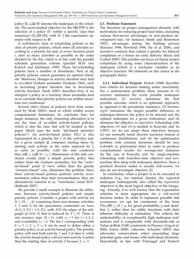
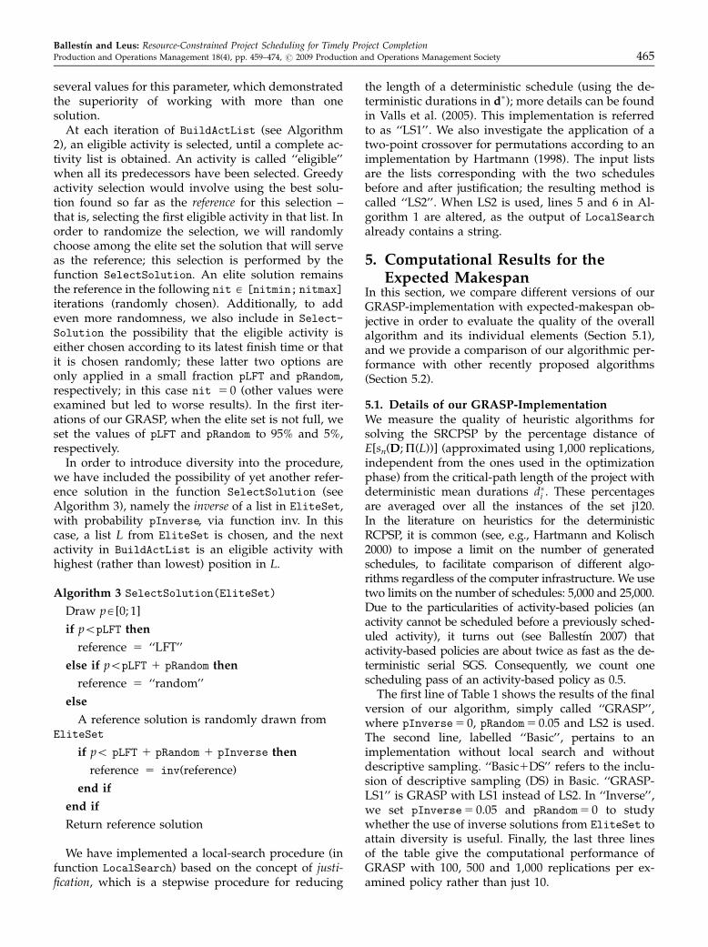
Finally, the inclusion of the DS also (slightly)improves the results of the basic algorithm. The im-provement in the average deviation from the critical-path length that is obtained by the incorporation of DS(compared with random sampling) was computed for5, 10 and 20 replications; the results for a schedulelimit of 5,000 and 25,000 schedules can be found inFigure 3. The gain obtained by DS tends to decrease asthe number of replications increases, both for 5,000and 25,000 schedules, and this trend is independent ofthe duration distribution. Specifically, the gainamounts to 2% with five replications for some distri-butions, making the incorporation of DS clearlyworthwhile. Based on the data presented so far, wecan recommend the use of descriptive rather thansimple random sampling in heuristic search especiallywhen the number of replications is low, in which casethe potential improvement appears to be significant.

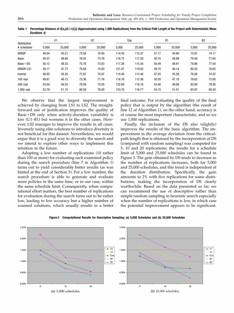
Table 1 Percentage Distance of E[sn(D;P(L))] (Approximated using 1,000 Replications) from the Critical-Path Length of the Project with Deterministic MeanDurations d �i

DistributionU1 U2 Exp B1 B2

# schedules 5,000 25,000 5,000 25,000 5,000 25,000 5,000 25,000 5,000 25,000

GRASP 46.84 45.21 72.58 70.95 114.42 112.37 47.17 45.60 75.97 74.17

Basic 50.57 48.68 76.55 74.78 118.72 117.20 50.70 48.99 79.49 77.64

Basic1DS 50.12 48.33 75.76 73.83 117.36 115.34 50.49 48.61 78.96 77.04

GRASP-LS1 49.17 47.73 76.68 74.93 121.07 119.02 49.75 48.14 80.50 78.62

Inverse 46.93 45.35 72.67 70.97 114.40 112.46 47.25 45.58 76.00 74.22

100 repl 49.81 46.73 75.36 71.76 116.76 112.36 50.20 47.18 78.63 75.00

500 repl 53.04 49.53 79.59 75.05 122.69 116.16 53.40 49.89 83.06 78.26

1,000 repl 53.79 51.15 80.50 76.95 123.70 118.77 54.15 51.51 83.97 80.28

Figure 3 Computational Results for Descriptive Sampling: (a) 5,000 Schedules and (b) 25,000 Schedules


Perhaps more important than the DS technique itselfis the fact that this confirms the value of researchregarding the implementation of the sampling in heu-ristic algorithms with replications, an observation thatwas also made by Gutjahr et al. (2000), and that is inline with earlier literature on the simulation of activitynetworks (Avramidis et al. 1991; Grant 1983; Sullivanet al. 1982).

In order to further justify the algorithmic designchoices for our GRASP-implementation, we includeTable 2, where we summarize our findings afterre-running the experiments that led to Table 1 on atotally different dataset. We used RanGen12 to gener-ate a dataset with ten scheduling instances with n 5 91and K 5 3 for each of the parameter settings: orderstrength OS 5 0.25, 0.50, 0.75; resource factor RF 5

0.45, 0.9; and resource constrainedness RC 5 0.3, 0.6(for more details about these parameters, we refer toDemeulemeester et al. 2003). We find that the attain-able solutions have makespans that are more distantfrom the critical-path length, leading to much higherdeviations than the ones in Table 1. This is not un-common, a similar behavior can be observed in Debelset al. (2006) for the RCPSP, where instances fromRanGen1 with 75 activities lead to a deviation of about270%, whereas for j120 a deviation of between30% and 35% was obtained. These results support therobustness of the algorithm, since the relative rankingof the different lines in the two tables is the same.The only difference is that inclusion of the inversealgorithm leads to slightly better results for U1, whichconfirms our suspicion that diversification can beworthwhile in some cases.

5.2. Comparison with State-of-the-Art AlgorithmsWe are now ready to compare our GRASP-algorithmwith other SRCPSP-algorithms from the literature.First of all, we consider the GA of Ballestın (2007),which uses the same dataset and schedule limit, withdistributions U1, U2 and Exp. Table 3 provides acomparison; we can see that GRASP outperforms the

GA in all cases. If we return to Tables 1 and 2, evenour Basic algorithm does better than the GA, whichhighlights the improvement obtained by adding thedescriptive sampling and LS2.

Secondly, we consider the tabu search (TS) andsimulated annealing (SA) procedures developedby Tsai and Gemmill (1998), who evaluate algorith-mic performance on the Patterson dataset (Patterson1984), with adaptations for obtaining stochastic (Beta)activity durations. As a measure of the quality of theiralgorithms, the authors report the deviation from anapproximate lower bound. Table 4 shows their results,obtained on a personal computer with 166 MHz; SA2and TS2 differ from SA1 and TS1 only in the param-eters settings; the two final columns contain theresults of our GRASP-algorithm on the same problemset. The GRASP-algorithm with a limit of 5,000 sched-ules outperforms both the SA and the TS in qualityand in time, even if we take into account the differ-ence in computer infrastructure. The small differencebetween 5,000 and 25,000 schedules might be due tothe fact that the solutions found are near-optimal.

Golenko-Ginzburg and Gonik (1997) test theiralgorithms on only one instance, which has 36 activ-ities and a single resource type; Table 5 contains theirand our results for this instance for three durationdistributions. The authors do not report running timesfor the procedures but only point out that the algo-rithm that uses an exact procedure to solveconsecutive multi-dimensional knapsack problems(Heuristic 1) needs much more time than the algo-rithm that solves these problems heuristically(Heuristic 2). Obviously, no strong conclusions can

Table 2 Percentage Distance of E[sn(D;P(L))] from the Critical-path Length of the Project with Deterministic Mean Durations for the RanGen-Dataset

DistributionU1 U2 Exp B1 B2

# schedules 5,000 25,000 5,000 25,000 5,000 25,000 5,000 25,000 5,000 25,000

GRASP 312.41 307.68 347.81 341.85 389.31 384.48 312.30 307.82 348.86 343.82

Basic 321.78 316.09 356.33 350.63 396.98 390.39 321.10 315.32 355.13 349.80

Basic1DS 319.78 314.15 353.43 348.30 394.82 388.63 320.43 314.75 354.95 349.29

GRASP-LS1 314.56 310.65 356.40 351.88 407.44 401.44 315.79 311.06 359.64 354.77

Inverse 311.59 307.61 347.41 342.67 389.97 384.66 312.65 307.87 349.39 344.68

100 repl 319.47 311.88 354.87 346.25 395.05 386.78 319.85 312.69 355.67 347.50

500 repl 328.75 321.57 364.11 357.45 405.50 398.76 329.02 322.14 365.45 358.57

1,000 repl 330.63 326.57 365.90 361.87 406.96 402.96 330.89 326.85 367.31 363.30

Table 3 Comparison Between GRASP and GA

DistributionU1 U2 Exp

# schedules 5,000 25,000 5,000 25,000 5,000 25,000

GA (%) 51.94 49.63 78.65 75.38 120.22 116.83

GRASP (%) 46.84 45.21 72.58 70.95 114.42 112.37


be drawn based on only one instance, but the differ-ence between the algorithms is quite large, especiallywith Heuristic 2. Stork (2001) also tests his exact al-gorithm (branch-and-bound) on the same instance,but only for the Uniform distribution. He obtains anexpected makespan of (rounded) 434 when thebranch-and-bound is truncated.

6. Correlations and Trade-OffsIn this section, we investigate how the different sta-tistics (expected makespan, probability of meeting adue date, etc.) behave relative to one another. In orderto approximate the correlations, we need a convenientsample of solutions. It is possible to generate a purelyrandom sample, but these frequently turn out to havea very large makespan, and obviously also a bad ser-vice level and tardiness. Therefore, we use Ballestın’s(2007) GA to generate a sample of solutions with ac-ceptable-to-good makespan values, which ensuressolutions for most ‘‘interesting’’ levels of the make-span (from ‘‘not good but not very bad either’’ to‘‘excellent’’). More specifically, we take the first 1,500solutions generated by the GA itself (after crossoverand mutation), the solutions in the initial populationare not included. We do not use the GRASP-algorithmthat is the subject of the first sections of this papersince this algorithm is used for all optimization runs,and we prefer to obtain all other information regard-ing the instances, such as due dates, correlations, etc.,by other means than via the algorithm of which theperformance is tested.

6.1. Expected Makespan Versus Service LevelThe first relationship to be examined is that betweenservice level and expected makespan, the first being aprobability, the second a measure of schedule length.It is tempting to simply investigate the correlation

between E[sn] and Pr[sn � d], for given values of d.This approach has some disadvantages, however.First of all, it is difficult to choose appropriate duedates d for an entire dataset: it may be more appro-priate to have (a) different value(s) per instance.Second, since the service level is expressed as apercentage, it is not the most convenient quantity torely on when computing correlations, because quite anumber of solutions may have 0% or 100% servicelevel. Therefore, we calculate for each instance the duedate d associated with given service levels and inves-tigate the correlation between d and E[sn] (so d is anestimate of a quantile, based on the order statistics ofthe makespan sample generated via the GA). Table 6contains the determination coefficient, which charac-terizes the linear relation between the two quantities(note that this coefficient is the square of the correla-tion coefficient).

We observe that the larger the variance, the smallerthe correlation: the distribution with the smallestcorrelation is clearly Exp, followed by U2 and B2. Thecorrelation is smallest in the tail and larger in the‘‘middle’’ of the domain. We conclude that, for mostpractical purposes, it is not necessary to work withservice levels: optimal (or good) expected-makespansolutions automatically perform very well on the ser-vice-level objective. Only perhaps in some extremecases will it be interesting to optimize the service levelinstead of the expected makespan, namely for veryhigh levels (� 99%) and large duration variability.One should also take into account that the smallercorrelations in these cases may be due in part to thedifficulty in estimating the service levels (simulationof rare events) (cf. Section 5, especially Figure 2).

As a result of the foregoing conclusion, service-levelbounds can be ignored as a representation of riskaverseness: assuming near-perfect correlation, eitherthe (unconstrained) solution with minimum expectedmakespan respects the service-level bound, or no

Table 5 Expected Makespan for the Instance from Golenko-Ginzburg andGonik (1997)

Distribution Beta Uniform Normal

Heuristic 1 433.88 448.49 448.85

Heuristic 2 447.98 461.35 461.58

GRASP (5,000) 408.75 427.64 422.04

GRASP (25,000) 403.16 424.28 415.40

Table 4 Comparison Between GRASP (with 5,000 and 25,000 Schedules)and the Algorithms of Tsai and Gemmill (1998)

Algorithm SA1 SA2 TS1 TS2

GRASP

(5,000)

GRASP

(25,000)

Above approximate

lower bound (%)

3.40 2.27 3.71 2.54 2.01 1.96

Average time (s) 10.804 21.414 5.834 11.290 0.92 4.24

Table 6 Determination Coefficients for the Relationship Between DueDate and Expected Makespan, for Four Service Levels (in the Firstcolumn): Average (First Value) and Standard Deviation (SecondValue) Over the Dataset

Probability U1 U2 Exp B1 B2

50% 99.91% 99.60% 97.66% 99.89% 99.45%

0.11 0.37 1.67 0.12 0.45

75% 99.84% 99.35% 96.94% 99.83% 99.22%

0.18 0.60 1.96 0.19 0.58

90% 99.62% 98.41% 93.81% 99.61% 98.21%

0.42 1.74 4.38 0.35 1.33

99% 98.21% 94.07% 73.91% 97.89% 92.62%

1.96 5.11 13.72 1.92 5.00

The columns correspond with the five duration distributions.


solution offers a service level above the threshold.One additional remark is in order here: as noted inSection 3, for comparable precision one needs a con-siderably higher number of replications for the servicelevel than for the expected makespan, so, other thingsbeing equal, the same number of replications can beexpected to favor the selection of better solutions inthe case of the makespan objective.

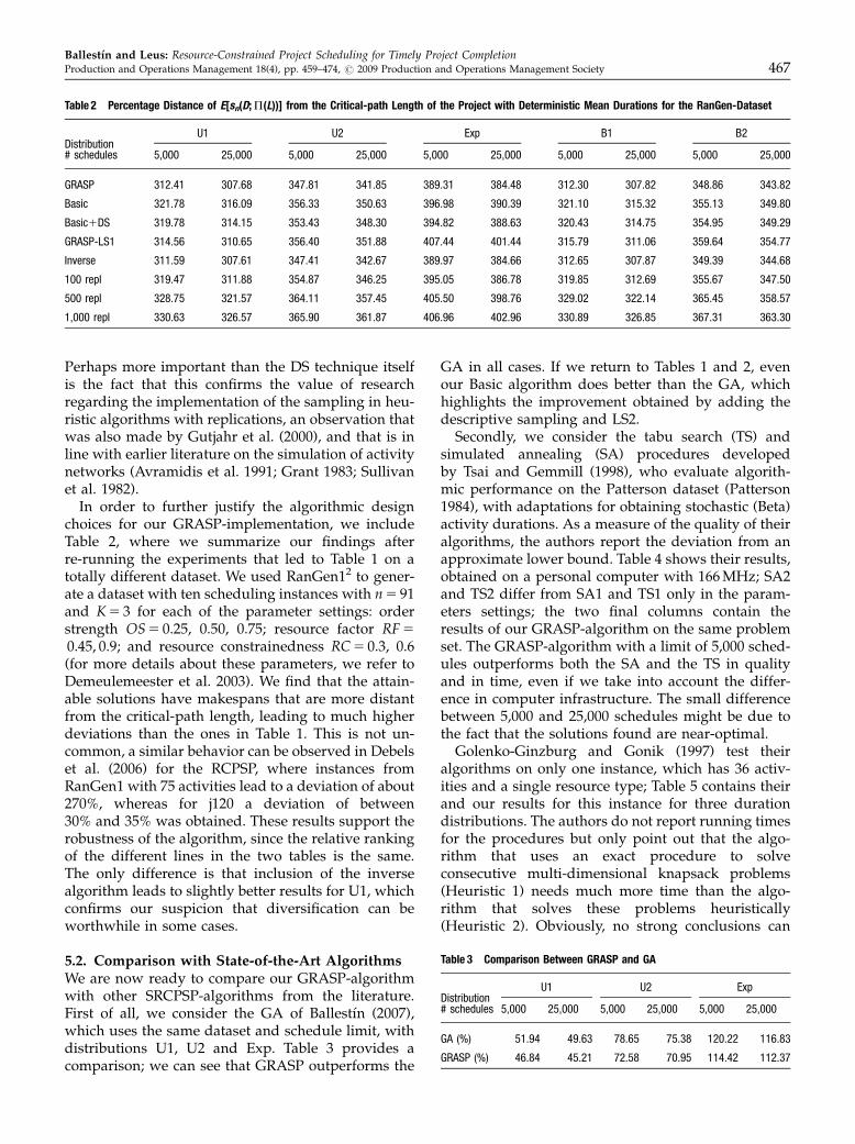
We are now ready to investigate the trade-off be-tween due date and service level. The results aredisplayed in Figure 4; in line with the previous para-graphs, optimal (or at least high-quality) service levelsare set via expected-makespan optimization. We ob-serve close similarities between the distributions withsimilar variance (U1–B1 and U2–B2). The graphs also‘‘flatten out’’ as variability increases. Specifically,the service level changes drastically when the dead-line changes for U1 and B1. For these low-variabilitydistributions, a clear ‘‘S’’-shape is discerned, whichshows that both for very high and very low servicelevels, the necessary improvement in average make-span to obtain a given service-level improvementis higher than in the ‘‘bulk’’ of the makespan spread,presumably because less solutions correspond to veryhigh and low makespans. The trend is almost linearfor U2, B2 and Exp, with the shallowest slope for Exp.These figures are averages over 600 instances, so thebehavior may be different for individual instances.

6.2. Expected Makespan Versus VarianceWe first include a discussion on delivery dates (Sec-tion 6.2.1) and then present computational results(Section 6.2.2).

6.2.1. Delivery Dates. For the benefit of riskaverseness, one of the options envisaged is toimpose lower bounds on the makespan variance. Inprinciple, we can simply eliminate a solution if it doesnot respect the constraint. A possible problem isthat, since our search procedure looks for objective-function improvements, it may generate onlynon-permissible solutions. We therefore proceed asfollows: the altered makespan salt

n corresponding withan activity list L is obtained as

saltn ðD;PðLÞÞ ¼ maxfsnðD;PðLÞÞ;Dg; ð1Þ

where D is an artificial delivery date for the schedule;higher D leads to higher expected makespan but lowervariance. For a given upper bound on the variance,we find the lowest value of D such that the boundis respected (via binary search). Since we evaluate theperformance measures by means of sampling,the computations corresponding with Equation (1)are straightforward (the max-operator is applied toknown numbers for each sample). As an example, forfour makespan realizations sn 5 100, 101, 103 and104, Table 7 contains the quantities salt

n ðd;PðLÞÞ. Oneactivity list leads to multiple pairs ðE½salt

n ;var½saltn Þ,

dependent on D. For a given threshold (upper bound)on the variance, however, only one of those pairscomes out best, namely the pair with lowest E½salt

n such that var½salt

n does not exceed the threshold.

6.2.2. Computational Results for the RelationshipVariance/Expected Makespan. In this section, weinvestigate the relationship between the expectedmakespan and the makespan variance. For the samedataset as in Section 6.1, we obtain results quitedifferent than before: average coefficients ofdetermination are between 62% and 69% (see Table8). Interestingly, the highest values occur for theExponential distribution, while these were lowest forthe service level (see Table 6). In part, the latterphenomenon may be due to the fact that theexpectation of an Exponential variable is equal to itsstandard deviation, so that for a given longest path ofactivities in the schedule, a higher expectation willalso imply a higher variance (although the same is

Figure 4 The Trade-off Between Due Date (Abscissa) and Service Level(Ordinate).

Five due dates are considered, namely min� (2/8)(max�min),min� (1/8)(max�min), min, min1(1/8)(max�min) andmin1(2/8)(max�min), where ‘‘min’’ and ‘‘max’’ are the lowestand highest makespan realization of a good GA-solution (for ahigh number of replications)

Table 7 Altered Makespan saltn Corresponding with Four Different Values

for the Delivery Date D

D

sn 99 100 101 106

100 100 100 101 106

101 101 101 101 106

103 103 103 103 106

104 104 104 104 106

Each column contains one sample of altered makespans.


true, but to a lesser extent, for the other distributions;in the context of resource-constrained scheduling, oneshould also generally avoid overly focusing onindividual paths in the precedence network).

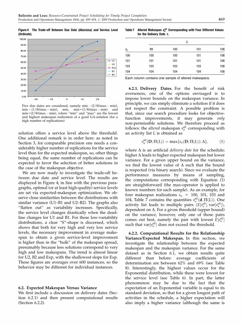
It can be concluded that these correlations are in-sufficiently high to neglect the variance, and weanticipate an actual expectation/variance trade-off.This trade-off is examined in Figure 5, where theexpected makespan obtained by the GRASP-algo-rithm is plotted as a function of an upper boundimposed on the variance (actually on the standarddeviation). The graphs are very similar in shape forall five distributions, but there are differences,mainly in the ‘‘jumps’’ in the expected makespancorresponding with a step from one k-value to thenext. For example, the jump for U1 is five units ofexpected makespan from k ¼ 1

4 to k 5 1, while it is 45for Exp. Consequently, the decision maker needs to‘‘sacrifice’’ a considerable increase in makespan ex-pectation if he/she wants to restrict the makespanvariance in cases where activity duration variance ishigh. However, this loss is negligible when the vari-ances of the Di are low, unless the restriction issevere (corresponding to low k-values). This obser-vation matches intuitive expectations, but has nowbeen demonstrated numerically as well.

6.3. Expected Makespan Versus Expected TardinessWe investigate the minimization of the expected tar-diness E½maxf0; sn � dg once the manager has fixed adeadline d. We are obviously mainly interested ind-values such that

mindfsnðd;PÞgodomax

dfsnðd;PÞg; ð2Þ

where optimization in the first and third term is per-formed over all possible duration-realization vectors din the sample used, and P is any activity-based policy(otherwise, we either have an optimal objective of zeroor we simply minimize expected makespan). In orderto examine these cases, we compute ‘‘minmin’’ as theminimum of the minimization term in Equation (2),taken over all policies P examined by the GA, andsimilarly ‘‘minmax’’ as the minimum of the maximiza-tion term in (2). We wish to investigate especiallydA]minmin; minmax[; other values often turn out to ad-mit policies with all makespan realizations eitherhigher or lower than the deadline. More specifically,we select three values for d, namely d1 5 minmin1

minmax� minmin)/2, d2 5 minmin15 minmax� minmin)/8 and d3 5 minmin13 (minmax� minmin)/4.

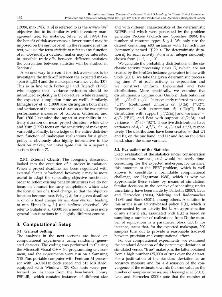
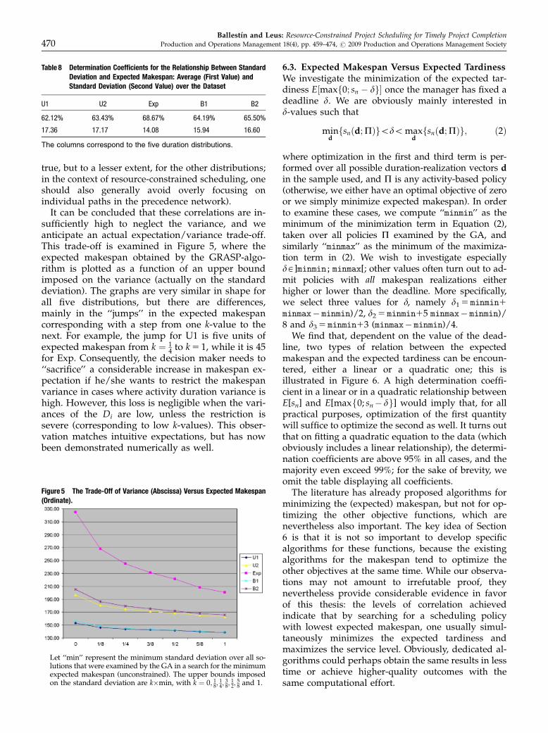
We find that, dependent on the value of the dead-line, two types of relation between the expectedmakespan and the expected tardiness can be encoun-tered, either a linear or a quadratic one; this isillustrated in Figure 6. A high determination coeffi-cient in a linear or in a quadratic relationship betweenE[sn] and E[maxf0; sn� dg] would imply that, for allpractical purposes, optimization of the first quantitywill suffice to optimize the second as well. It turns outthat on fitting a quadratic equation to the data (whichobviously includes a linear relationship), the determi-nation coefficients are above 95% in all cases, and themajority even exceed 99%; for the sake of brevity, weomit the table displaying all coefficients.

The literature has already proposed algorithms forminimizing the (expected) makespan, but not for op-timizing the other objective functions, which arenevertheless also important. The key idea of Section6 is that it is not so important to develop specificalgorithms for these functions, because the existingalgorithms for the makespan tend to optimize theother objectives at the same time. While our observa-tions may not amount to irrefutable proof, theynevertheless provide considerable evidence in favorof this thesis: the levels of correlation achievedindicate that by searching for a scheduling policywith lowest expected makespan, one usually simul-taneously minimizes the expected tardiness andmaximizes the service level. Obviously, dedicated al-gorithms could perhaps obtain the same results in lesstime or achieve higher-quality outcomes with thesame computational effort.

Table 8 Determination Coefficients for the Relationship Between StandardDeviation and Expected Makespan: Average (First Value) andStandard Deviation (Second Value) over the Dataset

U1 U2 Exp B1 B2

62.12% 63.43% 68.67% 64.19% 65.50%

17.36 17.17 14.08 15.94 16.60

The columns correspond to the five duration distributions.

Figure 5 The Trade-Off of Variance (Abscissa) Versus Expected Makespan(Ordinate).

Let ‘‘min’’ represent the minimum standard deviation over all so-lutions that were examined by the GA in a search for the minimumexpected makespan (unconstrained). The upper bounds imposedon the standard deviation are kmin, with k ¼ 0; 1

8;14;

38;

12;

58 and 1.


7. The Distribution of the MakespanRealizations of a Given Policy

In a deterministic setting, the decision maker knowsexactly when the project will be finished and canmake decisions based on this information. In a sto-chastic environment, he/she can only rely on theexpected makespan, which is a very limited piece ofinformation given that many different makespan re-alizations can actually occur. Clearly, knowledge ofthe entire distribution of possible makespan realizationsGðt;PðLÞÞ : R 7!½0; 1 : Gðt;PðLÞÞ ¼ Pr½snðD;PðLÞÞ � tis much more informative. Our goal in thissection is to better understand the shape of this distri-bution. Our first step is to calculate two descriptivemeasures for the shape and symmetry of a policy’smakespan distribution, its skewness and its kurtosis.Approximations for these values are collected in Table9. The first (second) line shows the average of the (ab-solute) skewness of the different instances. The thirdline represents the fraction of the instances with pos-itive skewness. The remaining lines display the sameresults for the kurtosis.

The data drawn from both Uniform distributionsare very symmetric, and even the number of instances

with positive and negative skewness is around 50%.The absolute value of the kurtosis is small, althoughthere are more instances in which the kurtosis is neg-ative. At any rate, if we pay attention to the absolutevalues, the data could stem from a Normal distri-bution (which has zero skewness and kurtosis). Inter-estingly, the increase in variability from U1 to U2hardly affects the measures. The situation is slightlydifferent for the Beta distributions: the B2 figures arevery similar to those of U1 and U2, but for B1 weobserve data that are less symmetric (long right-sidedtail), yet more unbiased in the case of positive andnegative skewness. We can still consider the Normaldistribution as a possible model for these data. Finally,the Exponential distribution data have a long right-sided tail (positive skewness) and a prominent peak(positive kurtosis). The Normal distribution shouldnot be able to capture these data.

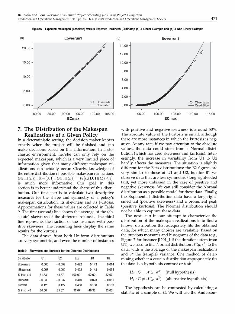
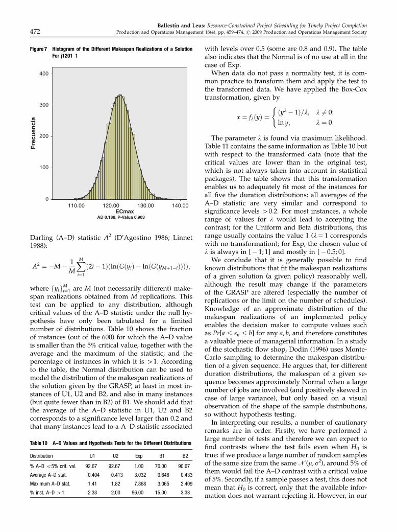
The next step in our attempt to characterize thedistribution of the makespan realizations is to find aknown distribution that adequately fits the obtaineddata, for which many choices are available. Based onthe previous measures and histograms of the data (e.g.,Figure 7 for instance j1201_1 if the durations stem fromU1), we tried to fit a Normal distribution N(m,s2) to thedata, with m the average of the makespan realizationsand s2 the (sample) variance. One method of deter-mining whether a certain distribution appropriately fitsthe data is a hypothesis contrast or test:

H0 : G ¼Nðm; s2Þ ðnull hypothesisÞH1 : G 6¼Nðm; s2Þ ðalternative hypothesisÞ:

The hypothesis can be contrasted by calculating astatistic of a sample of G. We will use the Anderson–

20.00

15.00

10.00

5.00

0.00

80.00 85.00 90.00 95.00 100.00 105.00

ECmax ECmax

Eoverrun1 Eoverrun3

ObservadaCuadrático

ObservadaCuadrático

14.00

12.00

10.00

8.00

6.00

4.00

2.00

0.00

95.00 100.00 105.00 110.00 115.00

(a) (b)

Figure 6 Expected Makespan (Abscissa) Versus Expected Tardiness (Ordinate): (a) A Linear Example and (b) A Non-Linear Example

Table 9 Skewness and Kurtosis for the Different Distributions

Distribution U1 U2 Exp B1 B2

Skewness 0.006 � 0.009 0.492 0.143 0.014

|Skewness| 0.067 0.069 0.492 0.148 0.074

% inst.40 51.33 43.67 100.00 92.00 52.67

|Kurtosis| � 0.030 � 0.037 0.440 0.023 � 0.051

Kurtosis 0.128 0.122 0.450 0.130 0.133

% inst.40 36.50 35.67 92.67 49.33 33.00


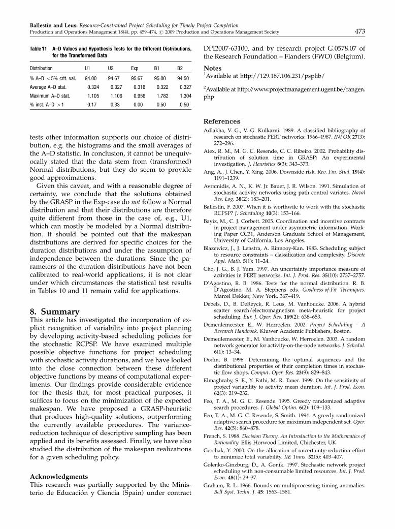
Darling (A–D) statistic A2 (D’Agostino 1986; Linnet1988):

A2 ¼ �M� 1

M

XMi¼1

ð2i� 1ÞðlnðGðyiÞ � lnðGðyMþ1�iÞÞÞÞ;

where fyigMi¼1 are M (not necessarily different) make-

span realizations obtained from M replications. Thistest can be applied to any distribution, althoughcritical values of the A–D statistic under the null hy-pothesis have only been tabulated for a limitednumber of distributions. Table 10 shows the fractionof instances (out of the 600) for which the A–D valueis smaller than the 5% critical value, together with theaverage and the maximum of the statistic, and thepercentage of instances in which it is 41. Accordingto the table, the Normal distribution can be used tomodel the distribution of the makespan realizations ofthe solution given by the GRASP, at least in most in-stances of U1, U2 and B2, and also in many instances(but quite fewer than in B2) of B1. We should add thatthe average of the A–D statistic in U1, U2 and B2corresponds to a significance level larger than 0.2 andthat many instances lead to a A–D statistic associated

with levels over 0.5 (some are 0.8 and 0.9). The tablealso indicates that the Normal is of no use at all in thecase of Exp.

When data do not pass a normality test, it is com-mon practice to transform them and apply the test tothe transformed data. We have applied the Box-Coxtransformation, given by

x ¼ flðyÞ ¼ðyl � 1Þ=l; l 6¼ 0;

ln y; l ¼ 0:

(

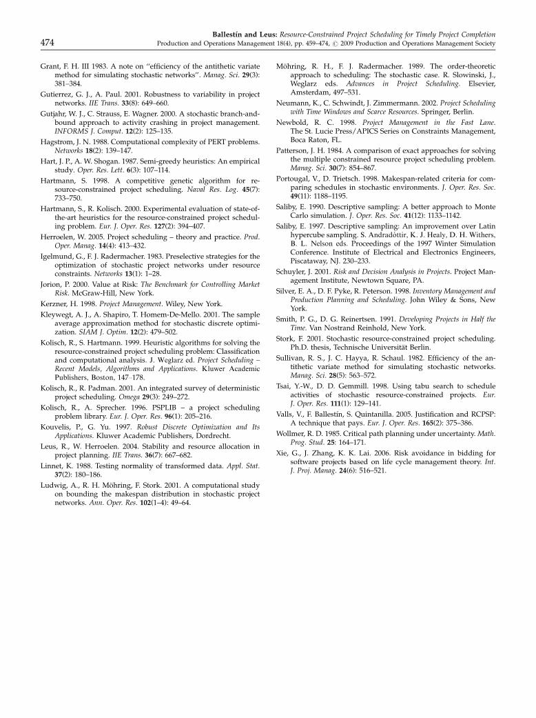
The parameter l is found via maximum likelihood.Table 11 contains the same information as Table 10 butwith respect to the transformed data (note that thecritical values are lower than in the original test,which is not always taken into account in statisticalpackages). The table shows that this transformationenables us to adequately fit most of the instances forall five the duration distributions: all averages of theA–D statistic are very similar and correspond tosignificance levels 40.2. For most instances, a wholerange of values for l would lead to accepting thecontrast; for the Uniform and Beta distributions, thisrange usually contains the value 1 (l5 1 correspondswith no transformation); for Exp, the chosen value ofl is always in [� 1; 1] and mostly in [� 0.5; 0].

We conclude that it is generally possible to findknown distributions that fit the makespan realizationsof a given solution (a given policy) reasonably well,although the result may change if the parametersof the GRASP are altered (especially the number ofreplications or the limit on the number of schedules).Knowledge of an approximate distribution of themakespan realizations of an implemented policyenables the decision maker to compute values suchas Pr[a � sn � b] for any a, b, and therefore constitutesa valuable piece of managerial information. In a studyof the stochastic flow shop, Dodin (1996) uses Monte-Carlo sampling to determine the makespan distribu-tion of a given sequence. He argues that, for differentduration distributions, the makespan of a given se-quence becomes approximately Normal when a largenumber of jobs are involved (and positively skewed incase of large variance), but only based on a visualobservation of the shape of the sample distributions,so without hypothesis testing.

In interpreting our results, a number of cautionaryremarks are in order. Firstly, we have performed alarge number of tests and therefore we can expect tofind contrasts where the test fails even when H0 istrue: if we produce a large number of random samplesof the same size from the same N(m,s2), around 5% ofthem would fail the A–D contrast with a critical valueof 5%. Secondly, if a sample passes a test, this does notmean that H0 is correct, only that the available infor-mation does not warrant rejecting it. However, in our

110.00 120.00 130.00 140.00

400

300

200

100

0

Fre

cuen

cia

ECmaxAD 0.188. P-Valua 0.903

Figure 7 Histogram of the Different Makespan Realizations of a SolutionFor j1201_1

Table 10 A–D Values and Hypothesis Tests for the Different Distributions


% A–D o5% crit. val. 92.67 92.67 1.00 70.00 90.67

Average A–D stat. 0.404 0.413 3.032 0.648 0.433

Maximum A–D stat. 1.41 1.82 7.868 3.065 2.409

% inst. A–D 41 2.33 2.00 96.00 15.00 3.33


tests other information supports our choice of distri-bution, e.g. the histograms and the small averages ofthe A–D statistic. In conclusion, it cannot be unequiv-ocally stated that the data stem from (transformed)Normal distributions, but they do seem to providegood approximations.

Given this caveat, and with a reasonable degree ofcertainty, we conclude that the solutions obtainedby the GRASP in the Exp-case do not follow a Normaldistribution and that their distributions are thereforequite different from those in the case of, e.g., U1,which can mostly be modeled by a Normal distribu-tion. It should be pointed out that the makespandistributions are derived for specific choices for theduration distributions and under the assumption ofindependence between the durations. Since the pa-rameters of the duration distributions have not beencalibrated to real-world applications, it is not clearunder which circumstances the statistical test resultsin Tables 10 and 11 remain valid for applications.

8. SummaryThis article has investigated the incorporation of ex-plicit recognition of variability into project planningby developing activity-based scheduling policies forthe stochastic RCPSP. We have examined multiplepossible objective functions for project schedulingwith stochastic activity durations, and we have lookedinto the close connection between these differentobjective functions by means of computational exper-iments. Our findings provide considerable evidencefor the thesis that, for most practical purposes, itsuffices to focus on the minimization of the expectedmakespan. We have proposed a GRASP-heuristicthat produces high-quality solutions, outperformingthe currently available procedures. The variance-reduction technique of descriptive sampling has beenapplied and its benefits assessed. Finally, we have alsostudied the distribution of the makespan realizationsfor a given scheduling policy.

AcknowledgmentsThis research was partially supported by the Minis-terio de Educacion y Ciencia (Spain) under contract

DPI2007-63100, and by research project G.0578.07 ofthe Research Foundation – Flanders (FWO) (Belgium).

Notes1Available at http://129.187.106.231/psplib/

2Available at http://www.projectmanagement.ugent.be/rangen.php

References

Adlakha, V. G., V. G. Kulkarni. 1989. A classified bibliography ofresearch on stochastic PERT networks: 1966–1987. INFOR 27(3):272–296.

Aiex, R. M., M. G. C. Resende, C. C. Ribeiro. 2002. Probability dis-tribution of solution time in GRASP: An experimentalinvestigation. J. Heuristics 8(3): 343–373.

Ang, A., J. Chen, Y. Xing. 2006. Downside risk. Rev. Fin. Stud. 19(4):1191–1239.

Avramidis, A. N., K. W. Jr. Bauer, J. R. Wilson. 1991. Simulation ofstochastic activity networks using path control variates. NavalRes. Log. 38(2): 183–201.

Ballestın, F. 2007. When it is worthwile to work with the stochasticRCPSP? J. Scheduling 10(3): 153–166.

Bayiz, M., C. J. Corbett. 2005. Coordination and incentive contractsin project management under asymmetric information. Work-ing Paper CC31, Anderson Graduate School of Management,University of California, Los Angeles.

Blazewicz, J., J. Lenstra, A. Rinnooy-Kan. 1983. Scheduling subjectto resource constraints – classification and complexity. DiscreteAppl. Math. 5(1): 11–24.

Cho, J. G., B. J. Yum. 1997. An uncertainty importance measure ofactivities in PERT networks. Int. J. Prod. Res. 35(10): 2737–2757.

D’Agostino, R. B. 1986. Tests for the normal distribution. R. B.D’Agostino, M. A. Stephens eds. Goodness-of-Fit Techniques.Marcel Dekker, New York, 367–419.

Debels, D., B. DeReyck, R. Leus, M. Vanhoucke. 2006. A hybridscatter search/electromagnetism meta-heuristic for projectscheduling. Eur. J. Oper. Res. 169(2): 638–653.

Demeulemeester, E., W. Herroelen. 2002. Project Scheduling – AResearch Handbook. Kluwer Academic Publishers, Boston.

Demeulemeester, E., M. Vanhoucke, W. Herroelen. 2003. A randomnetwork generator for activity-on-the-node networks. J. Schedul.6(1): 13–34.

Dodin, B. 1996. Determining the optimal sequences and thedistributional properties of their completion times in stochas-tic flow shops. Comput. Oper. Res. 23(9): 829–843.

Elmaghraby, S. E., Y. Fathi, M. R. Taner. 1999. On the sensitivity ofproject variability to activity mean duration. Int. J. Prod. Econ.62(3): 219–232.

Feo, T. A., M. G. C. Resende. 1995. Greedy randomized adaptivesearch procedures. J. Global Optim. 6(2): 109–133.

Feo, T. A., M. G. C. Resende, S. Smith. 1994. A greedy randomizedadaptive search procedure for maximum independent set. Oper.Res. 42(5): 860–878.

French, S. 1988. Decision Theory. An Introduction to the Mathematics ofRationality. Ellis Horwood Limited, Chichester, UK.

Gerchak, Y. 2000. On the allocation of uncertainty-reduction effortto minimize total variability. IIE Trans. 32(5): 403–407.

Golenko-Ginzburg, D., A. Gonik. 1997. Stochastic network projectscheduling with non-consumable limited resources. Int. J. Prod.Econ. 48(1): 29–37.

Graham, R. L. 1966. Bounds on multiprocessing timing anomalies.Bell Syst. Techn. J. 45: 1563–1581.

Table 11 A–D Values and Hypothesis Tests for the Different Distributions,for the Transformed Data


% A–D o5% crit. val. 94.00 94.67 95.67 95.00 94.50

Average A–D stat. 0.324 0.327 0.316 0.322 0.327

Maximum A–D stat. 1.105 1.106 0.956 1.782 1.304

% inst. A–D 41 0.17 0.33 0.00 0.50 0.50


http://129.187.106.231/psplib/a4.3d

http://www.projectmanagement.ugent.be/rangen.php



Grant, F. H. III 1983. A note on ‘‘efficiency of the antithetic variatemethod for simulating stochastic networks’’. Manag. Sci. 29(3):381–384.

Gutierrez, G. J., A. Paul. 2001. Robustness to variability in projectnetworks. IIE Trans. 33(8): 649–660.

Gutjahr, W. J., C. Strauss, E. Wagner. 2000. A stochastic branch-and-bound approach to activity crashing in project management.INFORMS J. Comput. 12(2): 125–135.

Hagstrom, J. N. 1988. Computational complexity of PERT problems.Networks 18(2): 139–147.

Hart, J. P., A. W. Shogan. 1987. Semi-greedy heuristics: An empiricalstudy. Oper. Res. Lett. 6(3): 107–114.

Hartmann, S. 1998. A competitive genetic algorithm for re-source-constrained project scheduling. Naval Res. Log. 45(7):733–750.

Hartmann, S., R. Kolisch. 2000. Experimental evaluation of state-of-the-art heuristics for the resource-constrained project schedul-ing problem. Eur. J. Oper. Res. 127(2): 394–407.

Herroelen, W. 2005. Project scheduling – theory and practice. Prod.Oper. Manag. 14(4): 413–432.

Igelmund, G., F. J. Radermacher. 1983. Preselective strategies for theoptimization of stochastic project networks under resourceconstraints. Networks 13(1): 1–28.

Jorion, P. 2000. Value at Risk: The Benchmark for Controlling MarketRisk. McGraw-Hill, New York.

Kerzner, H. 1998. Project Management. Wiley, New York.

Kleywegt, A. J., A. Shapiro, T. Homem-De-Mello. 2001. The sampleaverage approximation method for stochastic discrete optimi-zation. SIAM J. Optim. 12(2): 479–502.

Kolisch, R., S. Hartmann. 1999. Heuristic algorithms for solving theresource-constrained project scheduling problem: Classificationand computational analysis. J. Weglarz ed. Project Scheduling –Recent Models, Algorithms and Applications. Kluwer AcademicPublishers, Boston, 147–178.

Kolisch, R., R. Padman. 2001. An integrated survey of deterministicproject scheduling. Omega 29(3): 249–272.

Kolisch, R., A. Sprecher. 1996. PSPLIB – a project schedulingproblem library. Eur. J. Oper. Res. 96(1): 205–216.

Kouvelis, P., G. Yu. 1997. Robust Discrete Optimization and ItsApplications. Kluwer Academic Publishers, Dordrecht.

Leus, R., W. Herroelen. 2004. Stability and resource allocation inproject planning. IIE Trans. 36(7): 667–682.

Linnet, K. 1988. Testing normality of transformed data. Appl. Stat.37(2): 180–186.

Ludwig, A., R. H. Mohring, F. Stork. 2001. A computational studyon bounding the makespan distribution in stochastic projectnetworks. Ann. Oper. Res. 102(1–4): 49–64.

Mohring, R. H., F. J. Radermacher. 1989. The order-theoreticapproach to scheduling: The stochastic case. R. Slowinski, J.,Weglarz eds. Advances in Project Scheduling. Elsevier,Amsterdam, 497–531.

Neumann, K., C. Schwindt, J. Zimmermann. 2002. Project Schedulingwith Time Windows and Scarce Resources. Springer, Berlin.

Newbold, R. C. 1998. Project Management in the Fast Lane.The St. Lucie Press/APICS Series on Constraints Management,Boca Raton, FL.

Patterson, J. H. 1984. A comparison of exact approaches for solvingthe multiple constrained resource project scheduling problem.Manag. Sci. 30(7): 854–867.

Portougal, V., D. Trietsch. 1998. Makespan-related criteria for com-paring schedules in stochastic environments. J. Oper. Res. Soc.49(11): 1188–1195.

Saliby, E. 1990. Descriptive sampling: A better approach to MonteCarlo simulation. J. Oper. Res. Soc. 41(12): 1133–1142.

Saliby, E. 1997. Descriptive sampling: An improvement over Latinhypercube sampling. S. Andradottir, K. J. Healy, D. H. Withers,B. L. Nelson eds. Proceedings of the 1997 Winter SimulationConference. Institute of Electrical and Electronics Engineers,Piscataway, NJ. 230–233.

Schuyler, J. 2001. Risk and Decision Analysis in Projects. Project Man-agement Institute, Newtown Square, PA.

Silver, E. A., D. F. Pyke, R. Peterson. 1998. Inventory Management andProduction Planning and Scheduling. John Wiley & Sons, NewYork.

Smith, P. G., D. G. Reinertsen. 1991. Developing Projects in Half theTime. Van Nostrand Reinhold, New York.

Stork, F. 2001. Stochastic resource-constrained project scheduling.Ph.D. thesis, Technische Universitat Berlin.

Sullivan, R. S., J. C. Hayya, R. Schaul. 1982. Efficiency of the an-tithetic variate method for simulating stochastic networks.Manag. Sci. 28(5): 563–572.

Tsai, Y.-W., D. D. Gemmill. 1998. Using tabu search to scheduleactivities of stochastic resource-constrained projects. Eur.J. Oper. Res. 111(1): 129–141.

Valls, V., F. Ballestın, S. Quintanilla. 2005. Justification and RCPSP:A technique that pays. Eur. J. Oper. Res. 165(2): 375–386.

Wollmer, R. D. 1985. Critical path planning under uncertainty. Math.Prog. Stud. 25: 164–171.

Xie, G., J. Zhang, K. K. Lai. 2006. Risk avoidance in bidding forsoftware projects based on life cycle management theory. Int.J. Proj. Manag. 24(6): 516–521.


resource-constrained project scheduling for timely project completion with stochastic activity...

Documents