resource-aware task scheduling in wireless sensor networks · resource-aware task scheduling in...
TRANSCRIPT

Md. Muhidul Islam Khan,M.Sc.
Resource-Aware Task Scheduling inWireless Sensor Networks
DISSERTATION
to gain the Joint Doctoral Degree
Doctor of Philosophy (PhD)
————————————–
Alpen-Adria-Universitat Klagenfurt
Fakultat fur Technische Wissenschaften
in accordance with
The Erasmus Mundus Joint Doctorate in Interactive and Cognitive Environments
Alpen-Adria-Universitat Klagenfurt and Universita degli Studi di Genova
1. Begutachter: Univ.–Prof. Dr. techn. Bernhard RinnerInstitut fur Vernetzte und Eingebettete Systeme,
Alpen-Adria-Universitat Klagenfurt
2. Begutachter: Prof. Dr. Carlo S. RegazzoniDipartimento di Ingegneria Biofisica ed Elettronica,
Universita degli Studi di Genova
Klagenfurt, July 2014

Acknowledgments
This PhD Thesis has been developed in the framework of, and according to, the rules of the Erasmus
Mundus Joint Doctorate on Interactive and Cognitive Environments EMJD ICE [FPA n° 2010-0012] with
the cooperation of the following Universities:
Alpen-Adria-Universität Klagenfurt – AAU
Queen Mary, University of London – QML
Technische Universiteit Eindhoven – TU/e
Università degli Studi di Genova – UNIGE
Universitat Politècnica Catalunya – UPC
According to ICE regulations, the Italian PhD title has also been awarded by the Università degli Studi
di Genova.
This work has received funding from the EPiCS project (Engineering Proprioception in Computing
Systems) of the European Union Seventh Framework Programme under grant agreement no 257906.
i

First Reviewer
Univ.-Prof. Dr. techn. Bernhard Rinner
Institut fur Vernetzte und Eingebettete Systeme
Alpen-Adria-Universitat Klagenfurt, Austria
Second Reviewer
Prof. Dr. Carlo S. Regazzoni
Dipartimento di Ingegneria Biofisica ed Elettronica
Universita degli Studi di Genova
ii

Declaration of Honor
I hereby confirm on my honor that I personally prepared the present academic workand carried out myself the activities directly involved with it. I also confirm thatI have used no resources other than those declared. All formulations and conceptsadopted literally or in their essential content from printed, unprinted or internetsources have been cited according to the rules for academic work and identified bymeans of footnotes or other precise indications of source.
The support provided during the work, including significant assistance from my su-pervisors have been indicated in full.
The academic work has not been submitted to any other examination authority.The work is submitted in printed and electronic form. I confirm that the content ofthe digital version is completely identical to that of the printed version.
I am aware that a false declaration will have legal consequences.
Md. Muhidul Islam Khan Klagenfurt, July 25th, 2014
iii

Abstract
Wireless sensor networks (WSN) are an attractive platform for various pervasivecomputing applications. A typical WSN application is composed of different taskswhich need to be scheduled on each sensor node. However, the severe resourcelimitations pose a particular challenge for developing WSN applications, and thescheduling of tasks has typically a strong influence on the achievable performanceand energy consumption. In this thesis we propose different methods for schedulingthe tasks where each node determines the next task based on the observed ap-plication behavior. We propose a framework where we can trade the applicationperformance and the required energy consumption by a weighted reward functionand can therefore achieve different energy/performance results of the overall ap-plication. By exchanging data among neighboring nodes we can further improvethis energy/performance trade-off. We evaluate our approaches in a target track-ing application. Our simulations show that cooperative approaches are superior tonon-cooperative approaches for this kind of applications.
iv

Contents
1 Introduction 11.1 Motivation . . . . . . . . . . . . . . . . . . . . . . . . . . . . . . . . . 21.2 Challenges . . . . . . . . . . . . . . . . . . . . . . . . . . . . . . . . . 51.3 Contributions . . . . . . . . . . . . . . . . . . . . . . . . . . . . . . . 71.4 Thesis outline . . . . . . . . . . . . . . . . . . . . . . . . . . . . . . . 8
2 Background and related work 92.1 Wireless sensor networks . . . . . . . . . . . . . . . . . . . . . . . . . 92.2 Task scheduling . . . . . . . . . . . . . . . . . . . . . . . . . . . . . . 162.3 Online learning . . . . . . . . . . . . . . . . . . . . . . . . . . . . . . 182.4 Related work for task scheduling in WSN . . . . . . . . . . . . . . . . 20
2.4.1 Reinforcement learning method . . . . . . . . . . . . . . . . . 212.4.2 Evolutionary-based method . . . . . . . . . . . . . . . . . . . 212.4.3 Rule-based method . . . . . . . . . . . . . . . . . . . . . . . . 222.4.4 Constraint satisfaction method . . . . . . . . . . . . . . . . . 222.4.5 Market-based method . . . . . . . . . . . . . . . . . . . . . . 242.4.6 Utility-based method . . . . . . . . . . . . . . . . . . . . . . . 24
2.5 Difference to own approach . . . . . . . . . . . . . . . . . . . . . . . . 25
3 System model 273.1 Formal problem definition . . . . . . . . . . . . . . . . . . . . . . . . 273.2 System model . . . . . . . . . . . . . . . . . . . . . . . . . . . . . . . 29
3.2.1 Basic system model . . . . . . . . . . . . . . . . . . . . . . . . 293.2.2 System model for combinatorial auction . . . . . . . . . . . . 31
3.3 Set of actions . . . . . . . . . . . . . . . . . . . . . . . . . . . . . . . 313.4 Set of states . . . . . . . . . . . . . . . . . . . . . . . . . . . . . . . . 323.5 Reward function . . . . . . . . . . . . . . . . . . . . . . . . . . . . . . 33
4 Task scheduling methods 344.1 Combinatorial auction . . . . . . . . . . . . . . . . . . . . . . . . . . 344.2 Learning methods . . . . . . . . . . . . . . . . . . . . . . . . . . . . . 37
4.2.1 Reinforcement learning . . . . . . . . . . . . . . . . . . . . . . 374.2.2 Bandit solvers . . . . . . . . . . . . . . . . . . . . . . . . . . . 42
v

4.3 Task scheduling for target tracking . . . . . . . . . . . . . . . . . . . 434.3.1 Target tracking using combinatorial auction . . . . . . . . . . 434.3.2 Target tracking using cooperative Q learning . . . . . . . . . . 454.3.3 Target tracking using cooperative SARSA(λ) learning and
Exp3 bandit solvers . . . . . . . . . . . . . . . . . . . . . . . . 48
5 Implementation and Evaluation 565.1 Simulation environment . . . . . . . . . . . . . . . . . . . . . . . . . 565.2 Experimental setup . . . . . . . . . . . . . . . . . . . . . . . . . . . . 595.3 Simulation results . . . . . . . . . . . . . . . . . . . . . . . . . . . . . 59
5.3.1 Results of RL, CRL (one hop and two hop) . . . . . . . . . . 605.3.2 Results of cooperative Q learning . . . . . . . . . . . . . . . . 665.3.3 Results of combinatorial auction method . . . . . . . . . . . . 67
5.4 Comparison of RL, CRL, and Exp3 . . . . . . . . . . . . . . . . . . . 745.5 Discussion . . . . . . . . . . . . . . . . . . . . . . . . . . . . . . . . . 80
6 Conclusion and future work 816.1 Summary of contributions . . . . . . . . . . . . . . . . . . . . . . . . 816.2 Future works . . . . . . . . . . . . . . . . . . . . . . . . . . . . . . . 83
Bibliography 83
vi
List of Figures
1.1 Task scheduling in WSN . . . . . . . . . . . . . . . . . . . . . . . . . 6
2.1 Components of a wireless sensor node. . . . . . . . . . . . . . . . . . 102.2 Examples of some commercial sensor nodes. . . . . . . . . . . . . . . 112.3 Wireless sensor network. . . . . . . . . . . . . . . . . . . . . . . . . . 122.4 Overview of sensor applications [90]. . . . . . . . . . . . . . . . . . . 132.5 Data communication in a WSN [11]. . . . . . . . . . . . . . . . . . . 142.6 Task scheduling for better resource consumption/overall performance
trade-off. . . . . . . . . . . . . . . . . . . . . . . . . . . . . . . . . . . 172.7 Basic components of a reinforcement learning. . . . . . . . . . . . . . 20
3.1 WSN model components. Here four nodes ni, nj, nk, and nl. Ri
is the communication range, ri is the sensing range, and (ui, vi) isthe position of the node ni. Number of neighbors of the node ni,ngh(ni) = 2. . . . . . . . . . . . . . . . . . . . . . . . . . . . . . . . . 28
3.2 Proposed system model. . . . . . . . . . . . . . . . . . . . . . . . . . 303.3 System model for the combinatorial auction. . . . . . . . . . . . . . . 31
4.1 Target tracking example. Red dots denote the different positions ofa moving target at different time steps. Circles denote the sensingrange and black lines denote the communication link between thesensor nodes. . . . . . . . . . . . . . . . . . . . . . . . . . . . . . . . 45
4.2 Target prediction and intersection. Node j estimates the target tra-jectory and sends the trajectory information to its neighbors. Node ichecks whether the predicted trajectory intersects its FOV and com-putes the expected arrival time. . . . . . . . . . . . . . . . . . . . . . 49
4.3 Trajectory prediction and intersection. Black dots denote the trackedpositions of a target. The middle line is drawn based on linear re-gression. The other two lines are drawn by confidence interval. . . . . 53
4.4 State transition diagram. States change according to the value of twoapplication variables Nt and NET . Lc represents the local clock valueand Th1 is a time threshold. . . . . . . . . . . . . . . . . . . . . . . . 54
5.1 Simulation environment. . . . . . . . . . . . . . . . . . . . . . . . . . 58
vii

5.2 Achieved trade-off between tracking quality and energy consumptionfor β = 0.1. . . . . . . . . . . . . . . . . . . . . . . . . . . . . . . . . 61
5.3 Achieved trade-off between tracking quality and energy consumptionfor β = 0.3. . . . . . . . . . . . . . . . . . . . . . . . . . . . . . . . . 61
5.4 Achieved trade-off between tracking quality and energy consumptionfor β = 0.5. . . . . . . . . . . . . . . . . . . . . . . . . . . . . . . . . 62
5.5 Achieved trade-off between tracking quality and energy consumptionfor β = 0.7. . . . . . . . . . . . . . . . . . . . . . . . . . . . . . . . . 62
5.6 Achieved trade-off between tracking quality and energy consumptionfor β = 0.9. . . . . . . . . . . . . . . . . . . . . . . . . . . . . . . . . 63
5.7 Tracking quality versus energy consumption for various network sizes. 645.8 Randomness of target movement, η=0.1, 0.15, and 0.2 . . . . . . . . . 645.9 Randomness of target movement, η=0.25, 0.3, and 0.4 . . . . . . . . . 655.10 Randomness of target movement, η=0.5, 0.7, and 0.9 . . . . . . . . . 655.11 Cumulative reward over time by application scenario 1 (cp. Subsec-
tion 4.3.2). . . . . . . . . . . . . . . . . . . . . . . . . . . . . . . . . . 675.12 Tasks execution for Node A in Figure 4.1 by cooperative Q learning. . 685.13 Tasks execution for Node B in Figure 4.1 by cooperative Q learning. . 685.14 Tasks execution for Node C in Figure 4.1 by cooperative Q learning. . 695.15 Total number of execution for each action. . . . . . . . . . . . . . . . 695.16 Cumulative reward over time by application scenario 2 (cp. Subsec-
tion 4.3.2). . . . . . . . . . . . . . . . . . . . . . . . . . . . . . . . . . 705.17 Residual energy of the network over time. . . . . . . . . . . . . . . . 705.18 Variance of the available energy for different methods. . . . . . . . . . 715.19 Residual energy of the network. . . . . . . . . . . . . . . . . . . . . . 725.20 Tasks execution for Node A in Figure 4.1 by combinatorial auction
method. . . . . . . . . . . . . . . . . . . . . . . . . . . . . . . . . . . 725.21 Tasks execution for Node B in Figure 4.1 by combinatorial auction
method. . . . . . . . . . . . . . . . . . . . . . . . . . . . . . . . . . . 735.22 Tasks execution for Node C in Figure 4.1 by combinatorial auction
method. . . . . . . . . . . . . . . . . . . . . . . . . . . . . . . . . . . 735.23 Cumulative revenue of the network with three agents. . . . . . . . . . 745.24 Tracking quality/energy consumption trade-off for RL, CRL, and
Exp3 by varying the balancing factor of the reward function β. . . . . 765.25 Tracking quality/energy consumption trade-off for RL, CRL, and
Exp3 by varying the network size. . . . . . . . . . . . . . . . . . . . . 775.26 Tracking quality/energy consumption trade-off for RL, CRL, and
Exp3 by varying the randomness of target movement, η = 0.10, 0.15,and 0.20. . . . . . . . . . . . . . . . . . . . . . . . . . . . . . . . . . . 78
5.27 Tracking quality/energy consumption trade-off for RL, CRL, andExp3 by varying the randomness of target movement, η = 0.25, 0.30,and 0.40. . . . . . . . . . . . . . . . . . . . . . . . . . . . . . . . . . . 78
viii

5.28 Tracking quality/energy consumption trade-off for RL, CRL, andExp3 by varying the randomness of target movement, η = 0.50, 0.70,and 0.90. . . . . . . . . . . . . . . . . . . . . . . . . . . . . . . . . . . 79
5.29 Results varying the sensing radius . . . . . . . . . . . . . . . . . . . . 79
ix

List of Tables
1.1 Classification and examples of sensors [18]. . . . . . . . . . . . . . . . 2
4.1 Reward values for application scenario 1. . . . . . . . . . . . . . . . . 474.2 Reward values for application scenario 2. . . . . . . . . . . . . . . . . 48
5.1 Energy consumption of the individual actions. . . . . . . . . . . . . . 595.2 Comparison of RL, CRL, and Exp3 based on Tracking Quality (TQ),
Energy Consumption (EC), and Average Communication Effort (ACE)by varying the balancing factor of the reward function β. . . . . . . . 76
5.3 Mean and variance of the tracking quality and the energy consump-tion by varying the number of nodes, N=5, 10, and 20. Here TQmeans Tracking Quality and EC means Energy Consumption. . . . . 77
5.4 Comparison of average execution time and average number of trans-ferred messages (based on 20 iterations). . . . . . . . . . . . . . . . . 80
x

CHAPTER
1Introduction
In recent years, wireless sensor networks (WSN) have become an attractive platformfor observing real world phenomena. A WSN consists of hundreds or thousands oftiny sensor nodes capable of sensing, communicating wirelessly with their neighborsand performing on-board computation. Sensor nodes are small devices equippedwith one or more sensors, one or more transceivers, a processor, a storage deviceand actuators. Sensor nodes are typically powered by batteries which pose stronglimitations on energy but also on computation, storage and communication capabil-ities [50, 3].
Sensor networks perform a wide range of applications like area monitoring, mil-itary applications, target tracking, health and security, etc. Basically WSNs canbe applied to monitoring and computation-based applications [17]. Monitoring ap-plication includes fire detection, traffic monitoring, and wildlife habitat monitoring.Computation-based applications include target detection, tracking, and acoustic sig-nal processing which may require image processing and filtering operations.
WSNs applications require various kinds of independent tasks like sensing, trans-mitting, receiving, processing, etc., and various resources like processors, bandwidth,memory, battery power, etc. Each sensor node is responsible for performing a partic-ular task at each time step. Task execution consumes energy from the fixed energybudget of the sensor nodes. The scheduling of the individual tasks has a stronginfluence on achievable performance and energy consumption [60].
One of the important characteristics of a WSN is that the network changesdynamically over time. The network dynamics may happen because of node mobility,or because of node failure due to energy depletion. Energy consumption includesthe energy cost arising due to computation and communication tasks at each sensornode. In order to accommodate the dynamic nature of WSN, the need for adaptiveand autonomous task scheduling is well recognized [41].
In this thesis we focus on resource-aware task scheduling in WSN. Resource-aware, effective task scheduling is very important so that the WSN can know thebest task to execute during upcoming time slots. We propose different methodsfor online scheduling of tasks so that a better resource consumption/performance
1

CHAPTER 1. INTRODUCTION Page 2
trade-off is achieved.
1.1 Motivation
Recent technological advances have enabled the deployment of tiny, energy sensitivesensor nodes capable of local processing and wireless communication. Each battery-operated sensor node is able to perform limited processing. When sensor nodescommunicate with neighboring nodes and form a network they then have the abilityto measure a given physical environment in detail. Thus, a sensor network canbe described as a collection of sensor nodes that communicate with each other toperform application-specific actions [9].
Typically a sensor node has four basic components. Sensing components areresponsible for gathering data from the environment, processing components for dataprocessing, wireless communication components for data transmission and energysupply components for power supply to the sensor nodes [63]. Sensor nodes shouldbe chosen for an application depending on the physical phenomena to be monitoredlike temperature, pressure, light, humidity, etc. Table 1.1 shows the classificationand examples of some sensors.
Type ExamplesTemperature Thermistors, thermocouplesPressure Pressure gauges, barometers, ionization gaugesOptical Photodiodes, phototransistors, infrared sensors, CCD sensorsAcoustic Piezoelectric resonators, microphonesMechanical Strain gauges, tactile sensors, capcitive diaphragmsMotion, vibration Accelerometers, gyroscopes, photo sensorsFlow Anemometers, mass air flow sensorsPosition GPS, ultrasound-based sensors, infrared-based sensorsElectromagnetic Hall-effect sensors, magnetometersChemical pH sensors, electromechanical sensors, infrared gas sensorsHumidity Capacitive and resistive sensors, hygrometersRadiation Inonization detectors, geiger-Mueller counters.
Table 1.1: Classification and examples of sensors [18].
In some applications of WSNs, sensor nodes communicate directly with a central-ized controller or a base station. A WSN could be a collection of autonomous nodesthat communicate with each other by forming multi-hop radio networks and main-taining connectivity in an ad hoc manner. Such WSNs could change their topologydynamically, when the connectivity changes either to the mobility of nodes or to thefailure of nodes due to energy depletion [91].
A WSN monitors the environment by measuring the physical parameters likepressure, temperature, and humidity. Constant monitoring, detection of specific

CHAPTER 1. INTRODUCTION Page 3
events, military battlefield surveillance, object tracking, in-network data aggrega-tion, forest fire detection, flood detection, habitat exploration of animals, patientmonitoring, home appliances are some of the common applications in sensor net-works [2].
The number of nodes in a typical WSN is much higher than in a typical ad hocnetwork and dense deployment of these nodes is desired in a WSN to ensure thecoverage and connectivity. Sensor nodes must be cheap in order to make their hugenumbers. Sensor network hardware should be power-efficient and reliable in orderto maximize the lifetime of the network.
The lifetime of a WSN is extremely crucial for most applications. The lifetimeof the network depends on the energy consumed by the sensor nodes during theperformance of the different tasks required by the application. Typically sensornodes perform packet transmission, sensing, processing, and idle mode operation.Transmitting packets is the most energy-consuming task. Sensing and even in idlemode operation consume a consistent amount of power as well [30]. The lifetime ofthe network can be extended through energy efficient hardware and protocol design.Protocol helps to operate the sensor nodes based on the application demands.
For example, in a surveillance application, sensors (e.g., acoustic, video, seismic)are distributed throughout an area. The application will have some quality of ser-vice (QoS) or performance requirements like minimum percentage sensor coverage,minimum probability of missed detection of an event [79]. At the same time, theapplication needs to continue this performance as long as is possible with limitedbattery power, bandwidth, memory, etc. A careful design of the network protocolis required in order to maintain the trade-off between performance and resourceconsumption.
WSNs face some challenges and limitations in performing the application. Sensornetworks operate in an unattended fashion in remote geographic locations. Nodesmay be deployed in harsh and hostile environments. Wireless communication linksin a WSN operate in the radio, infrared, or optical range. To facilitate the globaloperation of WSNs, the selected transmission channel must be available worldwide.Deploying and managing a high number of sensor nodes in close proximity is achallenge. Any time after deployment, topology changes due to changes in sensornode position, power availability, dropouts, malfunctioning, jamming and so on. Asensor node may need to fit into a tight module on the order of 2cm×5cm×1cm oreven as small as a 1cm× 1cm× 1cm; a hardware constraint for developing a WSNapplications [74].
Wireless communications pose challenges to WSN design. An increasing distancebetween a sensor node and the base station increases the required transmission powerwhich is very energy consuming. Therefore, the distance is divided into severalshorter distances with multi-hop communication for sensor nodes protocols. Multi-hop communication requires cooperation among sensor nodes to identify efficientroutes and to serve as relays. Many sensor nodes use power-aware protocols whereradios are turned off when they are not in use [69].

CHAPTER 1. INTRODUCTION Page 4
The large scale and the energy constraints of WSNs make centralized algorithmsinfeasible. For example, in routing application, a base station can collect informationfrom all sensor nodes and inform each node of its route. On the other hand, indecentralized algorithms, sensor nodes cooperate with the neighboring nodes to makelocalized decisions.
Sensor nodes typically exhibit a strong dependency on battery life. Generally,sensor nodes use AA alkaline cells or one Li−AA cell. Energy consumption can beallocated to three functional domains: sensing, communication and data processing.
A performance metric is required to determine the performance of a particularapplication. Since energy-efficiency is the key characteristic of a WSN, the perfor-mance metric is typically associated with the trade-off between energy consumptionand performance of the application. For example, in a typical surveillance system,it may be required that one sensor node remains active in every sub-region of thenetwork. In this case, the performance metric can be determined by the percentageof the environment that is actually covered by the active sensors. In a typical track-ing application, the performance metric can be considered as the accuracy of targetlocation estimation provided by the network [61].
Generally a WSN node can perform the following tasks: transmit, receive, sleep,sense, data processing, etc. Each task requires a specific energy consumption level.Energy consumption in sense task is relevant to a specific application, while energyconsumption in other tasks are related to work process of a node [34]. In addition,energy consumption for the radio component in a node is much greater than thatof other components in the majority of WSN applications. Task scheduling helps tofind the best allocation of tasks to resources for the specific application by performingsome triggering activities. This triggering can be performed in several ways suchas offline, periodic, online or can be issued by changes in network. It also helps inlearning the usefulness of tasks in any given state to maximize the total amount ofreward over time [5].
For determining the next task to execute, the sensor nodes need to considerthe impact of each available task on energy budget and the application’s perfor-mance. There is a trade-off between application performance and resource con-sumption, and the task scheduler of the node should be able to adapt to changesin the environment. For example, in a target tracking application, sensor nodesshould frequently execute the tracking task when objects are within the field ofview (FOV). Since tracking is very resource consuming, this task should be avoidedwhen no object to track is nearby. Thus, task scheduling is an important issueto improve the energy/performance trade-off, and we investigate scheduling meth-ods which are able to learn effective scheduling strategies in dynamic environments.Since resource-awareness is an important aspect we consider energy consumption fortask scheduling and aim for low resource consumption of the scheduling algorithms.The ultimate goal is to achieve a high application performance while keeping theresource consumption low.
In this thesis we propose different methods of task scheduling. The proposed

CHAPTER 1. INTRODUCTION Page 5
methods help to learn the best task scheduling strategy based on previously observedbehavior and is further able to adapt to changes in the environment. A key step hereis to exploit cooperation among neighboring nodes, i.e., the exchange of informationabout the current local view of the application’s state. Such cooperation helps toimprove the trade-off between resource consumption and performance.
1.2 Challenges
As a WSN is a resource constrained network, there are challenges associated withtask scheduling. Figure 1.1 shows the basic task scheduling mechanism in WSN.Here we observe that there is an available resource infrastructure for the WSNapplication. Basically battery power, memory, and processing functionality formthe resource infrastructure. For performing the application, sensor nodes executesome tasks. Task scheduling methods help to schedule the tasks in a way thatthe resource is optimized with the goal of maximizing the lifetime of the network.Sensor nodes consume some resources from the resource budget for each executedtask. Scheduling can be performed online, offline or periodically.
Some of the challenges and design issues for task scheduling are as follows:
• Which task scheduling method to use?
– To select a suitable task scheduling method is a challenge. There areseveral methods for task scheduling (cp. Section 2.4 for more details).Due to the dynamic nature of WSNs, adaptive, and online task schedulingmethods should be chosen.
• How to monitor a resource assignment?
– Battery power, memory and processing functionality are the main re-sources of WSNs. We need to monitor the resources after executing thetasks. For example, a task execution consumes some energy from theenergy budget of the sensor node which has also an effect on the per-formance of the application. The goal is to maintain a better trade-offbetween energy consumption and application performance.
• How to model the WSN and application?
– To model the WSN with some number of nodes having different param-eters such as sensing radius, transmission radius, and resource consump-tion model is a challenge. These parameters provide an impact on taskscheduling. Tasks scheduling should meet the application demands. Forthat, careful consideration should be given to model the WSN and theapplication.

CHAPTER 1. INTRODUCTION Page 6
Avilable Resource Infrastructure
(Battery Power, Memory, Processing
Functionality)
Task Scheduling Methods
(Reinforcement Learning, Bandit
Solvers, Auction )
Goals
(Maximize
Lifetime of
the Network)
Trigger
(Online, Offline, Periodic)
Resource
Assignment Monitor
Figure 1.1: Task scheduling in WSN
• How to learn the best scheduling?
– There is a wide range of learning methods in computer science like super-vised learning, unsupervised learning, reinforcement learning, etc. Thechoice of a particular learning method is however a challenge since thereis no a priori information or a very little information exists for a dynamicsystem like WSNs.
• Which type of triggering should be used?
– Triggering for task scheduling can be performed online, offline or peri-odically. Appropriate triggering depends on the application and taskscheduling methods.

CHAPTER 1. INTRODUCTION Page 7
1.3 Contributions
The main contributions of this thesis are following:
• Perform research on state-of-the-art.
– We perform state-of-the art research on resource-aware task schedulingmethods in WSN. We find that most of the existing approaches do notprovide online scheduling of tasks. Further, they do not consider cooper-ation among neighboring nodes for task scheduling.
• Apply online learning methods for task scheduling.
– We apply online learning methods for task scheduling. We further con-sider the cooperation among neighboring nodes for task scheduling.
– We propose an online task scheduling method with cooperation amongneighboring nodes. First, we propose a cooperative Q learning, a variantof the reinforcement learning, for task scheduling. The main contributionhere is cooperation among neighboring nodes. This work is published in[41]. This is our initial work to apply reinforcement learning. We considera set of actions, a set of states, and scalar values for the reward. Weconsider a fixed topology with only three nodes in this work.
– We propose a market-based method for resource-aware task scheduling inWSN. We apply a combinatorial auction based method for task schedul-ing. We compare our proposed approach with static and random taskscheduling methods. Our proposed method outperforms the others, interms of residual energy, comparing with the existing static and randomtask scheduling. This work is published in [45].
– We update the work [41] with different topologies consisting of a dif-ferent number of nodes, weighted reward function, and exchanging dataamong neighboring nodes. We propose a cooperative reinforcement learn-ing (CRL), state-action-reward-state-action (SARSA(λ)) algorithm fortask scheduling. We compare our proposed method with independentreinforcement learning (RL) [67]. This work is published in [42].
– We propose a method using bandit solvers for task scheduling. We use theclassical adversarial algorithm, Exp3 (Exponential-weight algorithm forexploration and exploitation) for task scheduling. Exp3 and CRL achievesimilar results in terms of performance/resource consumption trade-off.The paper based on this study is currently under review [43].
• Evaluate/compare based on simulation.

CHAPTER 1. INTRODUCTION Page 8
– We evaluate RL, CRL, and Exp3 in terms of the performance/resourceconsumption trade-off. The paper based on this study is currently underreview [44].
1.4 Thesis outline
The remainder of this thesis is organized as follows:Chapter 2 offers an overview of the literature published in this area. In this
chapter, we provide background on wireless sensor networks (WSN), task scheduling,and online learning. We then review related works based on task scheduling in aWSN. We conclude this chapter with a discussion of the novelty of our work.
Chapter 3 provides the description of the system model. In this chapter, wedescribe the system model of our task scheduling methods. First, we delineatethe basic system model for our task scheduling followed by the system model forcombinatorial auction method. Afterward, we describe our considered set of actions,set of states, and the reward function.
Chapter 4 describes the proposed methods for the task scheduling in a WSN andthe task scheduling for the target tracking application. We describe the proposedresource-aware task scheduling methods for the WSN. Here, we consider the sys-tem model, the set of tasks, the set of states, and the reward function described inChapter 3. First, we describe the combinatorial auction method. Then we describethe cooperative reinforcement learning methods (Q learning, SARSA(λ)) and ban-dit solvers method. We conclude this chapter with a description of our proposedmethod for task scheduling in an object tracking application.
Chapter 5 shows the results and discussions. We describe our simulation en-vironment first. We apply reinforcement learning (RL), cooperative reinforcementlearning (CRL), exponential weight for exploration and exploitation (Exp3) banditsolvers, and combinatorial auction for the task scheduling in a WSN. We consider anobject tracking application and apply our methods for task scheduling. We evaluateour applied methods. We conclude this chapter with the discussion of simulationresults.
Chapter 6 concludes the thesis, summarizing the goals, contributions, results,and future work.

CHAPTER
2Background and relatedwork
In this chapter, we offer an overview of wireless sensor network (WSN), task schedul-ing, and online learning. We then proceed with related works based on tasks schedul-ing in WSN. We conclude this chapter with a discussion of the novelty of our work.
2.1 Wireless sensor networks
The recent promotion of micro-electro-mechanical systems (MEMS), digital electron-ics and wireless communication enable the evolution of low power, multifunctionalsensor nodes that are small in size and communicate with their neighbors. Wirelesssensor networks (WSN) consist of hundreds or thousands of small, battery-powered,and wireless devices called sensor nodes with on-board processing, communication,and sensing capabilities. Each node consists of one or more processors, multipletypes of memory, a wireless transceiver, a power source (e.g., batteries, solar cells),and diverse sensors [4].
Figure 2.1 shows the components of a general sensor node. Sensing elementsare a crucial part of a sensor node. Sensors collect information about physicalphenomena. Selecting the sensors for a particular application is a challenge. Forexample, if we propose to calculate distance using audio sensors, we will also needto measure humidity and temperature. Because the velocity of the sound dependsheavily on both temperature and humidity of the environment. The sensors have aparticular range to sense or detect the targets or events. This range is called sensingcoverage [91].
One of the components of a sensor node is the storage device. Depending on theoverall WSN structure, the requirement for storage devices at each node should bedifferent. For instance, if the WSN follows the structure that all sensor nodes shouldsend data to the central node then there is less importance for local storage on eachsingle sensor node. But if the goal is to reduce the amount of communication in thenetwork, local storage will be more significant. Flash storage, micro disks and nano-electronics based magnetoresistive random-access memory are some of the common
9

CHAPTER 2. BACKGROUND AND RELATED WORK Page 10
storage devices in WSN [82].
Figure 2.1: Components of a wireless sensor node.
Radios are the communication component of a sensor node. The design andselection of radios are important as the energy budget for sending and receivingmessages usually dominates the total energy budget of a sensor node. Radios have aparticular range called the radio coverage. Within the radio coverage, sensor nodescan communicate with each other [32]. Some low-power radio-based sensor devicesuse a single-channel RF transceiver operating at 916 MHz and some sensor sys-tems use a bluetooth-compatible 2.4 GHz transceiver with an integrated frequencysynthesizer.
Energy is the main constraint for a sensor node. So, power supply is a verysignificant factor. There are two different ways to address the concept of powersupplies. The foremost is to equip a sensor node with a source of energy. Presently,the most used option is to use high-density battery cells. Another alternative is toemploy the energy harvesting cells. The solar cell is one form of energy harvestingcells. Battery operation for sensors used in commercial applications is typicallybased on two AA alkaline cells or one Li− AA cell.
Processors are capable of on-board processing. Digital signal processor (DSP),field programmable gate array (FPGA) processor and application specific integratedcircuit (ASIC) are some examples of the processor. There are different microcon-trollers currently used in sensor node design such as Atmel AVR 8bit, Intel PXA271“Bulverde”, Texas Instruments MSP430, and Atmel AtMega 1281 [40].
Sensor nodes work together to monitor an area in order to obtain informationabout the environment. Based on the way of deployment of the nodes, there aretwo types of WSNs: structured and unstructured. In an unstructured WSN, sensor

CHAPTER 2. BACKGROUND AND RELATED WORK Page 11
nodes are densely deployed. Sensor nodes may be randomly placed into the field.After the deployment, the unstructured WSN is left unattended to perform theenvironment monitoring. Network maintenance is more difficult in an unstructurednetwork comparing with the structured network since there are so many nodes in anunstructured network. Sensor nodes are pre-determined to be located in specifiedlocations in a structured WSN. The advantage of a structured network is less networkmaintenance with less management cost [90].
Figure 2.2 shows some commercially available sensor nodes.
(a) Mica2 node [12]. (b) Mica2dot [37]. (c) Sun Spot [70].
(d) Smartdust node [39].
Figure 2.2: Examples of some commercial sensor nodes.
Figure 2.3 shows an example of a multi-hop data communication in a wirelesssensor network. The sensor node which detects an event, sends the information tothe neighboring nodes which terminates at a special node called the base station.The base station is like a gateway that connects one network to another. The basestation has enhanced capabilities as compared to simple sensor nodes. Here, a linkbetween two sensor nodes represents a single hop and that the data is eventuallytransferred via multiple hops to the base station.
When the transmission ranges of the radios of all sensor nodes are large enoughto communicate directly with the base station, each sensor node can send their datadirectly using a single-hop. However, most sensor networks cover a huge area andin this case radio transmission power should be kept minimum in order to make the

CHAPTER 2. BACKGROUND AND RELATED WORK Page 12
network energy efficient.
Figure 2.3: Wireless sensor network.
Basically, sensor network applications can be categorized into two types; monitor-ing the real world phenomena, and tracking targets. Monitoring applications includemilitary security detection, habitat monitoring, industrial monitoring, health andenvironmental monitoring. Habitat monitoring includes monitoring human habitats(smart homes and residential care centers, for instance), as well as animal habi-tats. Business monitoring includes inventory monitoring. Public/Industrial moni-toring includes structural, factory, inventory, machinery and chemical monitoring.Environmental monitoring includes weather, temperature and pressure monitoring.Tracking applications include tracking vehicles, humans, animals, and objects. Fig-ure 2.4 shows the overview of sensor applications [90].
A WSN has its own resource and design constraints. Resource constraints in-clude a limited energy, low bandwidth, limited processing capability of the centralprocessing unit, limited storing capacity of the storage device, and short commu-nication range. Design constraints are application-dependent and also depend onthe environment being monitored. The environment acts as a major determinantregarding the size of the network, deployment strategy, and network topology. Thenumber of sensor nodes or the size of the network changes based on the monitoredenvironment. For example, in indoor environments, fewer nodes are needed to forma network in a limited space, whereas outdoor environments may require more sensornodes to cover a huge unattended area. The deployment scheme also depends on theenvironment. Ad hoc deployment is preferred over a pre-planned deployment whenthe environment is not accessible and the network is composed of a vast number ofnodes [47].

CHAPTER 2. BACKGROUND AND RELATED WORK Page 13
Sensor Networks
Tracking Monitoring
Public/Industrial
Traffic Tracking
Car/Bus Tracking
Habitat
Animal Tracking
Military
Enemy
Tracking
Business
Human
Tracking
Military
Security
Detection
Habitat
Animal
Monitoring
Business
Inventory
Monitoring
Industrial
Structural
Monitoring
Factory
Monitoring
Machine
Monitoring
Chemical
Monitoring
Health
Patient
Monitoring
Environment
Weather
Monitoring
Figure 2.4: Overview of sensor applications [90].
Since sensor nodes operate on limited battery power, energy is a vital resourcefor a WSN. When a node is depleted of energy, it will disconnect from the network,which has a significant impact on the performance of the application.
One of the major reasons of energy consumption for the communication in WSNis idle mode consumption. When there is no transmission/reception, sensor nodesconsume some energy for listening and waiting for the information from the neigh-boring nodes. Over hearing is another source of energy consumption. Over hearingmeans that a node picks up packets that are destined for other nodes. Packetcollision is another issue of energy consumption. Collided packets should be re-transmitted which require extra effort in energy consumption. Protocol overhead is

CHAPTER 2. BACKGROUND AND RELATED WORK Page 14
also a reason for energy consumption.In some protocols, nodes are clustered together, to maintain scalability, that is;
to allow spatial expansion if necessary. In that case, there is a cluster head (CH)for each cluster. A CH is responsible for collecting data from the sensor nodes ofthat particular cluster. The CH can communicate with other CH and can send theprocessed information to the base station (BS). Both CH and BS are special typesof sensor nodes having more energy and processing functions [68]. Figure 2.5 showsthe basic data communication in a clustered WSN. Data communication can becategorized into two types: intra-cluster communication and inter-cluster commu-nication. In a particular cluster, sensor nodes communicating with the CH of thatcluster is called intra-cluster communication. CH communicating with the CH ofother clusters or with the BS is called inter-cluster communication.
Figure 2.5: Data communication in a WSN [11].
One of the factor that needs to be considered for network and protocol designin WSN is scalability. The number of sensor nodes deployed in the area may be inthe order of hundreds or thousands. A WSN must be designed so that the networkadapts to the number of sensor nodes. The node density depends on the WSNapplication. In an indoor environment, the number of sensor nodes could be smalleras compared to an unattended outdoor environment [73].
Fault tolerance is another factor to be considered. Some nodes may fail due topower failure, physical damage or monitored environmental interference. A WSNshould be fault tolerant. Fault tolerance depends on the application of WSN. If thesensor nodes are deployed in the home, there should be less consideration for faulttolerance since there should be less active, deliberate interference in an indoor envi-

CHAPTER 2. BACKGROUND AND RELATED WORK Page 15
ronments. On the other hand, if sensor nodes operate in a battlefield for surveillanceand detection then there should be proper care for fault tolerance because sensornodes may be damaged by hostile actions.
Production costs also need to be considered. Since a WSN consists of so manynodes, the production cost of a sensor node should be kept low. Current sensorsystems based on bluetooth technology cost about 10$. However, the cost of asensor node is generally targeted to be less than 1$, which is lower than the currentstate-of-the-art technology [36].
Network topology is another design factor for a WSN. A huge number of sensornodes are deployed over the monitored area and for this network topology is a chal-lenging factor. There are three issues related to topology maintenance. One issueis the deployment phase. Sensor nodes can be deployed by dropping from a plane,throwing by a catapult, placing in factories or by placing one by one either by ahuman or a robot. Post-deployment phase is another issue. After deployment, topol-ogy changes due to changes in position, available energy or malfunctioning. Anotherstage of network topology maintenance is re-deployment of additional nodes. Addi-tional sensor nodes may be deployed for replacing the malfunctioning nodes [54].
Sensor nodes are densely deployed which may be close to each other or maybe directly inside of the monitored phenomenon. Sensor nodes may work in busyintersections, in the interior of a large machinery, on the surface of the ocean during atornado, in a biological or chemical contaminated field, in a home or a large building,in a large warehouse, attached to animals, attached to fast moving vehicles, etc. [62]
Transmission media is another factor to be considered. Communicating nodesare linked by radio, infrared or optical media. For the global operation of WSN, thetransmission media should be available worldwide.
Data processing is another design factor for WSN. Energy spent in data pro-cessing is much less comparing with the data communication. Data processing inWSNs reduces the number of transmissions which minimizes the overall power con-sumption. This improves the performance and emergency response speed of theapplication of WSN like environmental monitoring [33]. For example, in sea waterquality monitoring application, number of sensor nodes distributed on the sea sur-face is large. If every nodes send the data to the base station for processing to findout the abnormality, there should be a huge number of data transmissions which isvery energy consuming. Each node able to do some local processing can reduce thisnumber of data transmissions and helps to make the system energy efficient [64].
Target tracking is a challenging, typical and generic application for WSN. Thetracking application may be for a single target or multiple targets. Targets maybe stationary or moving. Target tracking is applied in various applications ofWSN, such as the field of surveillance, finding intruder, military application, andtraffic operation. For target tracking application, the protocol design should beenergy efficient so that the better energy consumption/tracking performance isachieved [65] [4].

CHAPTER 2. BACKGROUND AND RELATED WORK Page 16
2.2 Task scheduling
In general, task scheduling means to make a plan for performing the tasks to achievean objective. Where each task has some constraints like completion time, requiredresources, etc. In computer science, this term basically used in the operating system(OS) concepts. Task scheduling in operating system is the method by which runningprocesses or programs are given access to the system resources, e.g., processor time,memory access, etc. Basically task scheduling is important for multi-tasking in OS.When the scheduler needs to perform multiple tasks in their queue to execute, thentask scheduling is required to meet the deadline. Whenever the processor becomesidle, the scheduler selects another task from the queue to perform next [86].
Basic task scheduling concepts can be categorized in to two types: preemptiveand non-preemptive task scheduling. The difference between preemptive and non-preemptive scheduling is that in non-preemptive scheduling, a process or a programenters the running state and is not removed from the processor until it is terminated.Preemptive scheduling allows the OS to control over the states of processes.
There are following five states which a process goes through during its life cycle.
• New: When a process is first activated and created. For example, launching asoftware program in OS.
• Ready: When the process is ready to be assigned to the processor.
• Running: When the process is being executed is known as “running”.
• Waiting:: The process is waiting for the communication from other processes.
• Terminated: When the execution of the process is finished.
Preemptive scheduling is when a process is interrupted and the processor is assignto another process with a higher priority. This type of scheduling occurs when aprocess switches from running state to a ready state or from a waiting state to readystate. Non-preemptive scheduling allows the process to run through to completionbefore moving onto the next task [77].
The basic non-preemptive scheduling mechanism is the first-in-first-out (FIFO).In this scheduling mechanism, the first task in the queue should be executed first.There is no priority to select the task from the queue.
Shortest-job-first (SJF) is a preemptive scheduling. In SJF, scheduler picks theshortest job that needs to be done, get it out of the way first and then pick the nextsmallest one and so on. Here the shortest job means, the job which requires theleast processor time or central processing unit (CPU) cycle [72].
Priority scheduling can be either preemptive or non-preemptive. In preemptivepriority scheduling, the scheduler preempt the processor if the priority of the newlyarrived process is higher than the priority of the currently running process. In non-preemptive priority scheduling, the scheduler simply puts the new process at the

CHAPTER 2. BACKGROUND AND RELATED WORK Page 17
head of the ready queue. Priorities are implemented using integers within a fixedrange, but there is no rule as to whether “high” priorities use large numbers or smallnumbers [88].
Round robin scheduling is another scheduling mechanism. It is similar to FIFOscheduling, except that CPU cycle are assigned with limits called time quantum.When a task is given the CPU, a timer is set to whatever value has been set fortime quantum. If the task finishes its cycle before the time quantum timer expires,the scheduler selects the next task from the queue and allocate CPU to it [48].
Task scheduling is an important aspect in WSN. Sensor nodes have no priorknowledge about which task to execute at each time step. Each node performstask scheduling among a set of available tasks. Scheduling is performed at timeinstances, when the previous task has terminated. Each task requires resources andcontributes to the overall performance of the application [20].
Figure 2.6 shows a small homogenous sensor network. Each sensor node needsto perform a particular set of tasks over time steps.
Node
Node
Node
Set of Tasks
to Perform
the
Application
Energy
Budget for
the Tasks
Cooperation Cooperation
Set of Tasks
to Perform
the
Application
Energy
Budget for
the Tasks
Set of Tasks
to Perform
the
Application
Energy
Budget for
the Tasks
Cooperation
Figure 2.6: Task scheduling for better resource consumption/overall performancetrade-off.
Every sensor node has an initial energy budget for performing tasks. Each taskconsumes an amount of energy budget and provides an impact to the overall perfor-mance. Here, cooperation means to share the local observations with the neighboringnodes. Tasks scheduling helps to schedule the tasks in a way that the better resource

CHAPTER 2. BACKGROUND AND RELATED WORK Page 18
consumption/overall performance is maintained.Task scheduling can be defined as to schedule a set of tasks needed for performing
the application in a way that the better resource consumption/application perfor-mance trade-off is achieved. For every application of WSN, there should be a set oftasks to be executed by each sensor node. These tasks can be scheduled offline oronline [7].
In offline scheduling, the complete information about the system activities isavailable a priori, and the schedule can be determined at compile time. Due to thehigh dynamics of WSN, complete system information is only available at runtimewhich requires online scheduling [52].
If we consider some sensor nodes scattered in a particular area for an objecttracking application, the network should work in such a way that it can efficientlyallocate its resources for the performance of its tasks. For object tracking the basictasks are sensing, transmitting, receiving, and sleeping. If we apply task schedulingfor object tracking, we need to model the network in such a way that it can maximizethe network lifetime.
2.3 Online learning
Online learning takes place in a sequence of rounds. At each round, the learner makessome kind of predictions and then receives some kind of feedback so that trainingand testing take place at the same time. Online learning is concerned with problemsof decision making about the present based on the previously earned experience andknowledge. Online learning is the process of answering questions given knowledgeof correct answers of previous questions. For that, the learner needs to make aprediction. This prediction mechanism is based on the mapping from the set ofquestions to the set of answers is called the hypothesis. After predicting the answer,the learner gets the correct answer of the question. The quality of the answer isthen evaluated by a loss function that measures the difference between predictedanswer and real answer [10]. Learning algorithms fall in to three groups based onthe feedback it has access to. These are supervised learning, unsupervised learning,and reinforcement learning.
In supervised learning, a learning algorithm analyzes the training data and pro-duces an inferred function, which can be used for mapping new examples. For ex-ample, a learning algorithm is given a problem to decide whether it will rain todayor not. For that, the learner was given a set of inputs about the raining probabilitiesof some days. At first, the learning algorithm needs to predict about an output (rainor not rain) based on the provided inputs. The quality of the prediction or answerof the learner is evaluated by the loss function. The learner’s ultimate goal is tominimize the cumulative loss [71].
In an unsupervised learning, the learner makes a decision based on past experi-ences by trail and error [75]. The learner simply receives inputs but obtains neither

CHAPTER 2. BACKGROUND AND RELATED WORK Page 19
supervised target outputs, nor rewards from the environment. However, it is possi-ble to develop the representations of the input that can be used for decision making,predicting future inputs, efficiently communicating the inputs to another machine,etc. [28]
The third category of learning is reinforcement learning. This is where the learnerreceives feedback about the appropriateness of its response. Reinforcement learningis one kind of online machine learning. In reinforcement learning, the learner learnsabout what to do (actions) and the mapping of situations to actions by the pastexperiences to maximize the reward over the long run. The learner is not told whichaction to perform like most of the machine learning mechanisms do. The learnerneeds to discover which actions provide the most reward by trying the actions.Actions not only provide an impact on the situation of the environment but also onobtained reward [38].
One of the challenges of reinforcement learning is exploration and exploitation ofthe actions. In reinforcement learning, the learner tries out all actions in it’s actionsset. Exploitation means to perform the action based on current information. Thelearner select the action which has been performed in the past, and found to beeffective in producing reward. Exploration means to perform a new action whichhas not been performed before. The learner needs to exploit actions in order toobtain reward, but the learner also needs to explore the actions in order to makebetter action selection in future [80].
A reinforcement learner generally has four basic components: a policy, a rewardfunction, a value function, and a model of the environment. The policy is thedecision making function of the agent. It specifies what action it should perform inwhich state it remains. The reward function maps the state of the environment toa single number indicating the gain of the state. The objective of the agent is tomaximize the total reward over long run. The value function defines what is goodin the long run. The model of the environment or external world should follow thebehavior of the environment. For a given situation and action, the model predictsthe resultant next state and next reward. Figure 2.7 shows the basic components ofreinforcement learning.
Due to the dynamic nature of WSN, it is necessary to schedule the tasks on-line [16]. We need a task scheduling mechanism that improves application perfor-mance. For example, for object tracking applications, sensor nodes need to performsome tasks over some time period. Sensing, transmitting, receiving, and sleepingare some of the common tasks performed by the sensor nodes. If sensor nodes havenothing to transmit/receive or sense then its better to turn off all the components.So, a task scheduling mechanism is required which is online and able to improvethe overall performance of the network. If we are able to learn efficiently and onlineabout the tasks to perform for a particular application then there should be betterperformance in terms of the resource consumption/performance trade-off [27].

CHAPTER 2. BACKGROUND AND RELATED WORK Page 20
Agent Environment
Agent’s Policy
(Tasks Scheduling Policy) Agent’s Value Function
Action
(Execution of a Task)
Reward
S
S
Figure 2.7: Basic components of a reinforcement learning.
2.4 Related work for task scheduling in WSN
In a resource constrained WSN, effective task scheduling is very important for facil-itating the effective use of resources [26]. Cooperative behavior among sensor nodescan be very helpful to schedule the tasks in a way that the energy is optimizedand also a considerable performance is maintained. Most of the existing methodsof tasks scheduling do not provide online scheduling of tasks. Most of them ratherconsider static task allocation instead of focusing on distributed task scheduling.The main difference between task allocation and distributed task scheduling is thattask allocation deals with the problem of finding a set of task assignments on a sen-sor network that minimizes an objective function such as total execution time [81].On the other hand, in a task scheduling problem, the objective is to determine thebest order of tasks execution for each sensor node. Each sensor node has to executea particular task at each time step in order to perform the application, and eachnode determines the next task to execute based on the observed application behav-ior and available resources. The following subsections describe some task schedulingmethods in WSN.

CHAPTER 2. BACKGROUND AND RELATED WORK Page 21
2.4.1 Reinforcement learning method
Reinforcement learning helps to enable applications with inherent support for ef-ficient resource/task management. It is the process by which an agent improvestask scheduling according to previously learned behavior. It does not need a modelof its environment and can be used online. It is simple, and demands minimalcomputational resources.
Shah et al. [66] consider Q learning as reinforcement learning for the task man-agement. They describe a distributed independent reinforcement learning approach(DIRL) for resource management, which forms an important component of any ap-plication includes initial sensor selection and task allocation as well as run-timeadaptation of allocated resources to tasks. Here the optimization parameters areenergy, bandwidth, network lifetime, etc. DIRL allows each individual sensor nodeto self schedule its tasks and allocate its resources by learning their usefulness in anygiven state while honoring application-defined constraints and maximizing the totalamount of reward over time. The advantage of using independent learning is thatno communication is required for coordination between sensor nodes and each nodeselfishly tries to maximize its own rewards. They apply this to the object trackingapplication and achieve better results in terms of the average award over time in thenetwork.
Shah et al. [67] presents a scheme for resource management in WSN using abottom up approach where each sensor node is responsible for task selection insteadof the top down approach conventionally used by other solutions. This bottomup approach using reinforcement learning allows development of autonomous WSNapplications with real time adaptation, minimal or no centralized processing require-ment for task allocation, and minimal communication overhead. They use two tierlearning: micro learning and macro learning, as used by each data stream sub-worldto steer the system towards application goal by setting/updating rewards for microlearners. They use collective intelligence (COIN) theory to enable macro learningthat can steer the system towards the application’s global goal.
2.4.2 Evolutionary-based method
Guo et al. [31] propose an evolutionary based method for the task allocation problemin WSN. They consider a WSN consists of m sensors and n independent task. Taskscompete for the sensors. The goal is to allocate n tasks to the sensors reasonably withthe shortest total execution time. They propose a basic particle swarm optimization(PSO) which is initialized with a population of random solutions. They consider aset of particles. Each particle is treated as a point with a velocity in a D dimensionalsolution space. Each particle has a fitness value which is set by an objective function.After calculating the fitness value, the system updates the local best value and thenglobal best value. For each particle, the system executes the mutation operator onthis particle if its diversity is less than the threshold. After that, the system executes

CHAPTER 2. BACKGROUND AND RELATED WORK Page 22
the mutation operator on the all particles if the population diversity is less than aparticular threshold. If the termination conditions are satisfied, then the methodterminates.
2.4.3 Rule-based method
A set of rules or predicates help to configure the wireless sensor networks, wherecertain functions must be automatically assigned to sensor nodes, such that theproperties of a sensor node (e.g. remaining energy, network neighbors) match therequirements of the assigned function. Based on the assigned rules, sensor nodesmay adapt their behavior accordingly, establish cooperation with other nodes, ormay even download specific code for the selected rule.
Frank et al. [26] propose a method for generic task allocation in wireless sensornetworks. They define some rules for the task execution and propose a role-rulemodel for sensor networks where “role” is used as a synonym for task. It is a pro-gramming abstraction of the role-rule model. This distributed approach provides aspecification that defines possible roles and rules for how to assign roles to nodes.This specification is distributed to the whole network via a gateway or alterna-tively it can be pre-installed on the nodes. A role assignment method takes intoaccount the rules and node properties, which may trigger execution and in networkdata aggregation. This generic role assignment approach does consider the energyconsumption but not the ordering of tasks to sensor nodes.
Liu et al. [55] mention a system for managing autonomic, parallel sensor systems.They consider energy a resource. They describe Impala, a middleware architecturethat enables application modularity, adaptability, and reparability in WSN. Impalaallows software updates to be received via each node’s wireless transceiver and tobe applied dynamically to the running system. In addition, Impala also provides aninterface for on-the-fly application adaptation in order to improve the performance,energy efficiency, and reliability of the software system. They consider the applica-tion parameters include recent histories, averages, or totals of the number of directnetwork neighbors encountered the amount of sensor data successfully transferredto peer sensor nodes, the amount of free storage for application data, and so on.System parameters include the battery level, the transmitter range, and the geo-graphic position of the nodes. They design the middleware considering some ruleson parameters. If the rules are satisfied then the next query is executed. This isdesigned to be a part of the Zebranet mobile sensor network. Impala is a lightweightrun-time system that can greatly improve the system reliability, performance andenergy efficiency.
2.4.4 Constraint satisfaction method
Constraint satisfaction is a formalism that is used to model a large class of problemswith applications in engineering design, planning, scheduling, resource allocation,

CHAPTER 2. BACKGROUND AND RELATED WORK Page 23
and fault diagnosis [19]. There are a number of variables, each of which has anassociated domain of values in a constraint satisfaction problem (CSP). Constraintsare specified on subsets of these variables restricting the set of values they can take onjointly. The objective of a CSP is to find out if each of these variables can be assigneda value from its domain in such a way that all the constraints are satisfied. In a CSPit suffices to find a single point in the search space which satisfies all constraints. ACSP is said to be satisfiable if there exists such a point and unsatisfiable otherwise.
Krishnamachari et al. [53] examine channel utilization as a resource managementproblem by constraint satisfaction. They consider a wireless sensor network of nnodes placed randomly in a square area with a uniform, independent distribution.This work tests three self configuration tasks in wireless sensor networks: partitioninto coordinating cliques, formation of Hamiltonian cycles and conflict free channelscheduling. They explore the impact of varying the transmission radius on thesolvability and complexity of these problems. In the case of partition into cliques andHamiltonian cycle formation, they observe that the probability that these tasks tobe performed undergoes a transition from zero to one. Almost every network graphis generated by random location of the nodes satisfies the desired global property.In these cases, the critical transmission range corresponds to an energy efficientoperating point. However, in the third task (conflict free channel scheduling) theyobserve that the transition occurs in reverse; there is a critical transmission rangebelow which almost all network graphs generated by the random location of nodescan be allocated the available number of channels, and beyond which the desiredproperty is rarely satisfied.
Kogekar et al. [51] consider energy or power saving as a resource managementproblem modeled by dynamic software reconfiguration. It is a constraint guided ap-proach for dynamic reconfiguration in WSN. Reconfiguration is performed by tran-sitioning from one point of the operation space to another based on the constraints.System requirements are expressed as formal constraints on operational parameterssuch as power consumption, latency, accuracy, and other QoS properties that aremeasured at run-time. In this work, once a new configuration that satisfies all theconstraints are found, the reconfiguration can be accomplished by online softwaresynthesis targeting an interpreted language or a command interface. The reconfig-urator is responsible for performing the necessary local application changes uponnotification from the base station. Here each mote has two components: monitorand reconfigurator. monitor observes the existing resources such as remainingbattery power. The base station has four components: GlobalConstraintMonitor,GRATISP lus, DESERT and GRATIS. The monitor of each mote reports itsremaining battery power to global constraint monitor of the base station whose hasa database to check the energy level of that mote is sufficient to keep the existenceconfiguration. If the energy level is below a certain threshold then it reports the pa-rameters to GRATISP lus which sends the design space representation as an inputto the DESERT . DESERT configures the design and sends it to the GRATIS,and finally the reconfigurator of a mote gets direction about configuration from

CHAPTER 2. BACKGROUND AND RELATED WORK Page 24
GRATIS. They implement it to track the movement of people across an aisle.
2.4.5 Market-based method
An auction is a market mechanism for allocating resources. The essence of anauction is a game, where the players are the bidders, the strategies are the bids andboth allocation and payments are functions of the bids. One well known auctionis the Vickery-Clarke-Groves (VCG) auction [49], which requires gathering globalinformation from the network and performing centralized computations.
Huang et al. [14] describe the signal to noise ratio (SNR) auction and the powerauction that determine the relay selection and relay power allocation in a distributedfashion. Here the network rate (bps/Hz) is considered as a resource. The proposedauction-based resource allocation methods can be generalized to networks with mul-tiple relays. Each relay announces a price and a reserve bid, without knowing theprices and reserve bids of other relays of others relays. Each user submits a non-negative bid vector, one component for each relay. Based on the bids, the relayallocates to the user transmission power. The Nash equilibrium [59] is achieved ina distributed fashion if it allows the users to iteratively update their bids based onbest response functions in an asynchronous fashion. They implement this on a singlerelay network.
Chen et al. [35] address the problem of providing congestion-management forwireless sensor networks executing several target tracking applications. They con-sider information or data as resource. They employ auctions to provide two differentutility loss management solutions: equalizing utility loss across all tracking applica-tions and minimizing the total utility loss of applications. Any time a given nodehas multiple target report packets for different applications to be forwarded for itscurrent transmission slot, the node conducts an auction to assign the slot to thepacket with the highest bid. Hence, the bidders represent packets awaiting trans-mission and their bids are defined by the predicted information utility loss of theapplications to which packets are sent. This in turn prevents resource starvation ofany auction participant.
2.4.6 Utility-based method
The utility-based technique is a valuable tool for resource management in wirelesssensor networks (WSN). The benefits of this technique include the ability to takeapplication utilities into account for performing the application.
Dhanani et al. [21] give a comparison of utility-based information managementpolicies in sensor networks. Here the resource is information or data. They considertwo models: sensor centric utility-based (SCUB) and resource manager (RM) mod-els. SCUB is a distributed approach that instructs individual sensors to make theirown decisions about what sensor information should be reported, based on a utilitymodel for data. RM is a consolidated approach that takes into account knowledge

CHAPTER 2. BACKGROUND AND RELATED WORK Page 25
from all sensors before making decisions. They evaluate these policies through simu-lation in the context of dynamically deployed sensor networks in military scenarios.Both SCUB and RM can extend the lifetime of a network comparison to the networkwhich is not maintaining any policy. Without any policy, the network can send moreinformation than SCUB and RM but it has less network lifetime compared to these.RM networks last longer than SCUB according to their experiment.
Byers et al. [13] describe utility-based decision making in wireless sensor network.They consider application domains in which a large number of distributed, networkedsensors must perform a sensing task repeatedly over time. They present a model forsuch application in which they define appropriate global objectives based on utilityfunctions and specify a cost model for energy consumption. They derive the utilityfrom a consumer of sensor network resources by a monotone function U : S → [0, 1],which for a network graph G = (V,E) maps the sensing subset, the set of all nodesin the graph that are sensing, to a real valued interval. In a best effort service model,nodes attempt to optimize the utilization of resources in the present without regardto future cost. With the goal of optimizing the total utility derived over the lifetimeof the network, the model enables nodes to discount current gain to optimize theirconsumption of energy over time
2.5 Difference to own approach
The following is a brief overview of the differences between the state-of-the-art andour own approach.
• Most of the existing methods [31], [26], [55], [51], [21] of task scheduling inWSNs do not provide online scheduling of tasks. They mainly consider statictask allocation instead of focusing on task scheduling. The main differencebetween task allocation and task scheduling is that task allocation deals withthe problem of determining a set of task assignments on a sensor network thatminimizes an objective function such as the total execution time [81]. On theother hand, the objective of task scheduling is to determine the best temporalorder of tasks for each sensor node. In offline scheduling, the complete infor-mation about the system activities are available a priori, and the schedule canbe determined at compile time. Due to the high dynamics of WSN, completesystem information is only available at runtime and so online scheduling isrequired [52]. We propose online learning methods for task scheduling.
• Most of the existing methods of task scheduling in WSNs [29], [53], [21] nei-ther consider distributed tasks scheduling nor the trade-off among resourceconsumption and performance. They also do not explicitly consider energyconsumption. We consider the trade-off among resource consumption andperformance.

CHAPTER 2. BACKGROUND AND RELATED WORK Page 26
• Shah et al. [66] introduce a task scheduling approach for WSN based on anindependent reinforcement learning method (RL) for online task scheduling.They use Q learning [85] for the task scheduling. Their approach relies ona simple and fixed network topology consisting of three nodes and a staticvalue for the reward function. They further consider neither any cooperationamong neighbors nor the energy/performance trade-off. Our approach hassome similarity with [66], but is much more general and flexible since we sup-port general WSN topologies, a more complex reward function for expressingthe trade-off between energy consumption and performance, and cooperationamong neighbors.
• Most of the existing methods do not evaluate task scheduling methods. Weevaluate three online task scheduling methods: Reinforcement Learning (RL),Cooperative Reinforcement Learning (CRL), and Exponential Weight for Ex-ploration and Exploitation (Exp3). Each of these three are evaluated for taskscheduling in a target tracking application, and analyzed in terms of theirperformance (a trade-off between tracking quality and energy consumption).Our proposed approach also takes cooperation into consideration, where eachnode sharing local observations with its neighbors.

CHAPTER
3System model
In this chapter, we describe the system model of our task scheduling methods.We apply reinforcement learning (RL), cooperative reinforcement learning (CRL),exponential weight for exploration and exploitation (Exp3) bandit solvers, and com-binatorial auction for the task scheduling in a WSN. We consider a target trackingapplication and apply our methods for task scheduling. First, we delineate the basicsystem model for our task scheduling followed by the system model for combina-torial auction method. Afterward, we describe our considered set of actions, set ofstates, and the reward function.
3.1 Formal problem definition
Before describing the problem formally, terms like resource consumption, and track-ing quality need to be defined. In WSNs, resource consumption happens due to per-form the various tasks needed for the application. Each task consumes an amount ofenergy from the fixed energy budget of the sensor nodes. Typically, tracking qual-ity in a target tracking application of a WSN is defined as the accuracy of targetlocation estimation provided by the network.
In our approach the WSN is composed by N nodes represented by the setN = {n1, . . . , nN}. Each node has a known position (ui, vi) and a given sensingcoverage range which is simply modeled by circle with radius ri. All nodes withinthe communication range Ri can directly communicate with ni and are referred toas neighbors. The number of neighbors of ni is given as ngh(ni). The availableresources of node ni is modeled by a scalar Ei. We consider the battery power ofsensor nodes as resource. We consider a set of tasks to perform over time steps. Eachtask consumes some battery power from the energy budget of the sensor nodes. Weconsider a set of static values for the energy consumption of tasks. These values areassigned based on the energy demands of the task. We set higher value for the taskswhich need higher energy consumption.
The WSN application is composed by A tasks (or actions) represented by the
27

CHAPTER 3. SYSTEM MODEL Page 28
set A = {a1, . . . , aA}. Once a task is started at a specific node, it executes for aspecific (short) period of time and terminates afterwards. Each task execution on aspecific node ni requires some resources Ej and contributes to the overall applicationperformance P . Thus, the execution of task aj on node ni is only feasible if Ei ≥ Ej.The overall performance P is represented by an application specific metric. On eachnode, an online task scheduling takes place which selects the next task to executeamong the A independent tasks. The task execution time is abstracted as fixedperiod. Thus, scheduling is required at the end of each period which is representedas time instant ti. We consider non-preemptive scheduling based on our proposedmodel. Figure 3.1 shows our considered WSN model components.
Figure 3.1: WSN model components. Here four nodes ni, nj, nk, and nl. Ri is thecommunication range, ri is the sensing range, and (ui, vi) is the position of the nodeni. Number of neighbors of the node ni, ngh(ni) = 2.
We demonstrate our task scheduling approach using a target tracking applica-tion. We consider a sensor network which may consists of a variable number ofnodes. The sensing region of each node is called the field of view (FOV). Everynode aims to detect and track all targets in the FOV. If the sensor nodes would per-form tracking all the time then this would result in the best tracking performance.

CHAPTER 3. SYSTEM MODEL Page 29
But executing target tracking all time is energy demanding. Thus, task should onlybe executed when necessary and sufficient for tracking performance. Sensor nodescan cooperate with each other by informing neighboring nodes about “approaching”targets. Neighboring nodes can therefore become aware of approaching targets.
We define the objective function in a way that we can trade the application per-formance and the required energy consumption by a balancing factor. The ultimateobjective for our problem is to determine the order of tasks on each node such thatthe overall performance is maximized while the resource consumption is minimized.Naturally these are conflicting optimization criteria, so there is no single best solu-tion. The set of non-dominating solutions for such a multi-criteria problem can betypically represented by a Pareto front.
3.2 System model
We apply reinforcement learning methods (cooperative Q learning, SARSA(λ)),bandit solvers (Exp3), and a combinatorial auction method for task scheduling.First, we describe the basic system model for reinforcement learning methods, andbandit solvers then we describe the system model for the combinatorial auctionmethod. Since reinforcement learning methods, and bandit solvers both consider aset of tasks, a set of states, and a reward for the executed actions, the system modelis same for both methods. On the other hand, in combinatorial auction method,there should be some consideration of bids, auctioneer, and revenues. Due to thedifferent components in the system, we consider two different system models.
3.2.1 Basic system model
The task scheduler operates in a highly dynamic environment, and the effect ofthe task ordering on the overall application performance is difficult to model. Wetherefore apply reinforcement learning methods, and bandit solvers to determine the“best” task order given the experiences made so far. Figure 3.2 depicts our proposedsystem model can be described as follows:
• Agent: Each sensor node embeds an agent which is responsible for executingthe online learning algorithm.
• Environment: The WSN application represents the environment in our ap-proach. Interaction between the agent and the environment is achieved byexecuting actions and receiving a reward function.
• Action: An agent’s action is the currently executed application task on thesensor node. At the end of each time period ti each node triggers the schedulerto determine the next action to execute.

CHAPTER 3. SYSTEM MODEL Page 30
• State: A state describes an internal abstraction of the application which istypically specified by some system parameters. In our target tracking applica-tion, the states are represented by the number of currently detected targets inthe node’s FOV, and expected arrival times of targets detected by neighboringnodes. The state transitions depend on the current state and action.
Figure 3.2: Proposed system model.
• Policy: An agent’s policy determines what action will be selected in a par-ticular state. In our case, this policy determines which task to execute atthe perceived state. The policy can focus more on exploration or exploitationdepending on the selected setting of the learning algorithm.
• Value function: This function defines what is good for an agent over the longrun. It is built upon the reward function values over time and hence its qualitytotally depends on the reward function [66].
• Reward function: This function provides a mapping of the agent’s state and thecorresponding action to a reward value that contributes to the performance.We apply a weighted reward function which is capable of expressing the trade-off between energy consumption and tracking performance.
• Cooperation: We consider the information exchange among neighboring nodesas cooperation. The received information may influence the application’s stateof a sensor nodes.
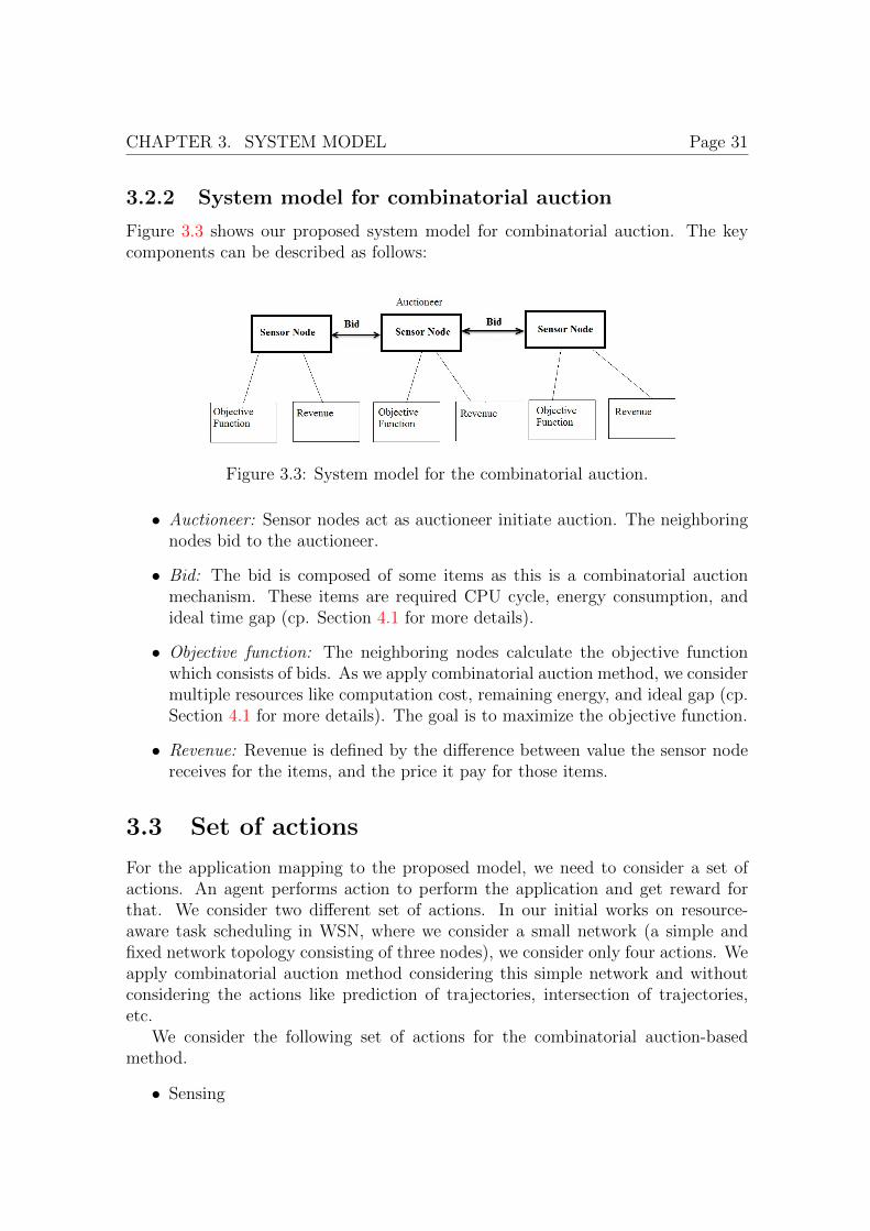
CHAPTER 3. SYSTEM MODEL Page 31
3.2.2 System model for combinatorial auction
Figure 3.3 shows our proposed system model for combinatorial auction. The keycomponents can be described as follows:
Figure 3.3: System model for the combinatorial auction.
• Auctioneer: Sensor nodes act as auctioneer initiate auction. The neighboringnodes bid to the auctioneer.
• Bid: The bid is composed of some items as this is a combinatorial auctionmechanism. These items are required CPU cycle, energy consumption, andideal time gap (cp. Section 4.1 for more details).
• Objective function: The neighboring nodes calculate the objective functionwhich consists of bids. As we apply combinatorial auction method, we considermultiple resources like computation cost, remaining energy, and ideal gap (cp.Section 4.1 for more details). The goal is to maximize the objective function.
• Revenue: Revenue is defined by the difference between value the sensor nodereceives for the items, and the price it pay for those items.
3.3 Set of actions
For the application mapping to the proposed model, we need to consider a set ofactions. An agent performs action to perform the application and get reward forthat. We consider two different set of actions. In our initial works on resource-aware task scheduling in WSN, where we consider a small network (a simple andfixed network topology consisting of three nodes), we consider only four actions. Weapply combinatorial auction method considering this simple network and withoutconsidering the actions like prediction of trajectories, intersection of trajectories,etc.
We consider the following set of actions for the combinatorial auction-basedmethod.
• Sensing

CHAPTER 3. SYSTEM MODEL Page 32
• Transmit
• Receive
• Sleeping
We consider the following actions for a target tracking application using re-inforcement learning methods, and bandit solvers (cp. Subsection 4.3.3 for moredetails).
• Detect Targets
• Track Targets
• Send Message
• Predict Trajectory
• Goto Sleep
• Intersect Trajectory
3.4 Set of states
Another component for application mapping is a set of states. Agents execute anaction for performing the application and shift from one state to another. States aredefined by application variables. We consider some application variables to definethe state. These application variables can change for executing a particular action.As the varibales change, agent can shift from one state to another after executing thetask. We consider the following variables to represent the states for the reinforcementlearning method, SARSA(λ), and bandit solvers (cp. Subsection 4.3.3 for moredetails).
• Currently detected targets.
• List of expected arrival times of targets.
Based on these variables, we abstract the target tracking application by threestates (cp. Subsection 4.3.3 for more details).
• Idle: This state denotes that there is currently no target detected within thenode’s FOV and the local clock is too far from the expected arrival time ofany target already detected by some neighbors.
• Awareness: There is currently no detected target in the node’s FOV in thisstate. However, the expected arrival time of at least one target is less than athreshold value.

CHAPTER 3. SYSTEM MODEL Page 33
• Tracking: This state indicates that there is currently at least one detectedtarget within the node’s FOV.
We consider the following set of variables for the cooperative Q learning.
• Currently detected targets.
• Minimum energy required for actions.
• Data to transmit.
3.5 Reward function
The reward function is another component for application mapping. For performingeach action, sensor nodes receive a reward. This reward helps to take decision infuture that which task is suitable to execute at each time step.
In our proposed reinforcement learning methods, and bandit solvers, we considera weighted reward function which balances between performance and resource con-sumption. Performance is measured by the ratio of the number of tracked positionsof the target inside the FOV of the node to the number of all possible detectedtarget’s positions in the FOV. Resource consumption is defined as the energy con-sumption at each time step for executing the tasks. We consider a balancing factorwhich balances the trade-off between energy consumption and tracking quality (cp.Subsection 4.3.3 for more details).
For cooperative Q learning methods, we consider scalar values for the rewardsof each action. Higher scalar values are set to the tasks of lower energy requirement(cp. Subsection 4.3.2 for more details).

CHAPTER
4Task scheduling methods
In this chapter, we describe the proposed resource-aware task scheduling methods ina WSN. Here, we consider the system model, the set of tasks, the set of states, andthe reward function described in Chapter 3. First, we describe the combinatorialauction method. Then we describe the cooperative reinforcement learning methods(Q learning, SARSA(λ)), and the bandit solvers method. We apply our methodsin a target tracking application. We also describe the task scheduling in a targettracking application using our proposed methods in this chapter.
4.1 Combinatorial auction
We consider a market-based approach for the task scheduling in WSN. We usecombinatorial auction-based method here as our bid is composed of some items likecentral processing unit (CPU) cycle, energy requirement, and ideal time gap. Targettracking is considered as application here. We consider two application variables todefine the states of the system which are field of view (FOV) and data to transmit(DTT). Both of these variables can take the value either 1 or 0. For example, whenDTT=1 then there is data to transmit. When two application variables FOV andDTT of a particular node i become 1, then the node acts as an auctioneer. Weconsider four tasks sensing, transmit, receive, and sleeping for the target trackingapplication. Each task needs some items, e.g., CPU cycle, energy, and ideal timegap to execute. The targets are sold in this auction. The auctioneer initiatesan auction. The neighboring nodes send bid to the auctioneer and calculate theobjective function to win.
Objective function is as follows
Objective(j) = αSj +β
ηj+
γ
Dj(4.1)
where the node j has the signal strength for detecting Sj, the node with highersignal strength carries more information about the target. The resource price ηj,
34

CHAPTER 4. TASK SCHEDULING METHODS Page 35
the node with lower resource price should be given priority as the node can performa task with lower resource price can maintain the resource efficiency in the systemand the term Dj defines the distance between the target and the node. α, β and γare equilibrium constants. The resource price ηj in Equation 4.1 can be calculatedby the following parameters.
• Required CPU cycle (RCPU): It refers to the expected CPU cycle required foraccomplishing the task.
• Available CPU: It is sensor node’s CPU clock frequency.
• Computation Cost: It can be calculated by the following equation that is usedin [23].
CompCost(RCPU , f) = NCV 2dd + Vdd(I0e
VddnVT )(
RCPU
f) (4.2)
f ∼= K(Vdd − c) (4.3)
where VT is the thermal voltage, and C, I0, n, K, c are processor dependentparameters.
• Remaining energy (E): It refers to the remaining energy of the sensor node.
• Ideal gap (TIG): It is a gap between the time that sensor nodes accomplishthe task and the time that sensor nodes communicate the tasks output to itsneighbor. If the ideal gap is very large, the incentive for the task would ratherdecrease.
The resource price is calculated by the following equation
ηj = (CompCost
E)× exp(TIG) (4.4)
where CompCost refers to computation cost, E refers to remaining energy and TIGmeans ideal gap. After calculating the resource price, the sensor nodes will bid forthe object to track it.
Now we need an algorithm that will find out the winner and the bids that willmaximize the revenue of each agent as we consider the sensor nodes here as agentsin a multi-agent environment. We use the combinatorial auction named ProgressiveAdaptive User Selection Environment (PAUSE) auction method [84].
The agents maintain a set B of the current best bids, each consists of a set ofitems. The agents also maintain price of the items agent i should pay bvalue, value ofthe bids vi(b
items), and value for the items of the bids bitems. There are two variablesg∗ and u∗. g∗ is the revenue of the agent and u∗ is the winner bid values. There aretwo other variables my bids and their bids to track the bid values. At any point in

CHAPTER 4. TASK SCHEDULING METHODS Page 36
Algorithm 1 PAUSEBID (i)
1: Inputs: Price of the items agent i should pay bvalue, Value of the bids vi(bitems),
Value for the items of the bids bitems
2: Output: Revenue of the agent g∗, Winner bid values W3: Initialization: my bids← φ, their bids← φ, g∗ ← φ, u∗ ← (W )4: for b ∈ B do5: if bagent = i or vi(b
items) > bvalue then6: Set my bids← my bids+ new bid(i, bitems, vi(b
items))7: else8: their bids← their bids+ b9: end if
10: for S ∈ subsets of fewer items such that vi(S) > 0 do11: Set my bids← my bids+ new bid(i, S, vi(S))12: bids← my bids+ their bids13: MAXIMUM(bids, φ)14: u∗ ← (W )15: surplus←
∑bagent=i
W (bitems)− bvalue
16: if surplus = 0 then17: return g∗
18: end if19: my payment← vi(b
items)− bvalue20: for b ∈ u∗|bagent = i do21: if my payment ≤ 0 then22: g∗ ← 023: else24: g∗ ← W (bitems) +my payment.W (bitems)−bvalue
surplus
25: end if26: end for27: end for28: end for29: return g∗
30: MAXIMUM(bids, g)31: for each iteration do32: Sort the bids in increasing order33: N = bid1, bid2, ...., bidn34: for i = 1 to n do35: Set g ← the list of bids in increasing order.36: end for37: end for

CHAPTER 4. TASK SCHEDULING METHODS Page 37
the auction, there will also be a set W ⊆ B of currently winning bids. This is theset of bids that currently maximizes the revenue, where the revenue of W is givenas follows
g∗ ← W (bitems) +my payment.W (bitems)− bvalue
surplus(4.5)
where W (bitems) is the value of the winning bids, my payment is defined by the valueit receives for the items minus the price it must pay for those items, my payment←vi(b
items) − bvalue. surplus is defined by the difference of the winning bid valuesminus the price it should pay for those items. The goal of the bidding agents in thePAUSE auction is to maximize their revenue.
Given an agent’s value function and current set of winning bids W , we cancalculate the agent’s utility from W as
ui(W ) =∑
b∈W |bagent=i
Vi(bitems − bvalue) (4.6)
That is, the agents utility for a bid set W is the value it receives for the items itwins in W minus the price it must pay for those items. If the agent is not winningany items then its utility is zero. The goal of the bidding agents in the PAUSEauction is to maximize their utility.
4.2 Learning methods
We need suitable methods for learning resource-aware task scheduling. Learningmethods help to learn the next suitable task to execute based on the past observedbehavior. The learning methods could be offline or online. Due to the dynamicnature of a WSN, we do not have any a priori information about the schedulingof tasks. So, our target is to learn the scheduling online. Reinforcement learningmethods, bandit solvers, are online learning methods for task scheduling. By thesemethods, it is possible to learn the best task to execute from the past experienceswhich provide more reward. We choose reinforcement learning methods and banditsolvers for learning task scheduling online and to get the better trade-off betweenresource consumption and performance.
4.2.1 Reinforcement learning
Reinforcement learning is a branch of machine learning and is concerned with de-termining an optimal policy (cp. Section 2.3 for more details). It maps the statesof the environment to the actions that an agent should take in those states so as tomaximize a numerical reward over time. We propose cooperative Q learning for taskscheduling. Here this is cooperative in a sense that each sensor node sends the valuefunction to the neighbors. We also consider a weight factor [89] for the neighbors. Asour aim is to learn task scheduling in a cooperative manner we choose cooperative

CHAPTER 4. TASK SCHEDULING METHODS Page 38
Q learning. We propose cooperative state-action-reward-state-action, SARSA(λ)learning algorithm. Here we also consider the cooperation among neighboring nodeswith the local observations. We also consider the weight factor for the neighboringnodes. Here λ is the learning parameter which helps for guaranteed convergencelearning [80].
Cooperative Q learning for task scheduling
Cooperative Q learning is a reinforcement learning approach to learn the usefulnessof some tasks over time in a particular environment. We consider the wirelesssensor network as a multi-agent system. The nodes correspond to agents in themulti-agent reinforcement learning. The world surrounding the sensor nodes formsthe environment. Tasks are considered as activities for the sensor nodes at eachtime step such as transmit, receive, sleep, sense, etc. States are formed by set ofsystem variables such as object in the FOV of sensor nodes, required energy fora specific action, data to transmit, etc. A reward value provides some positive ornegative feedback for performing a task at each time step. Value functions definewhat is good for an agent over long run described by reward function and someparameters. In cooperative Q learning every agent needs to maintain a Q matrix forthe value functions like independent Q learning. Initially all entries of the Q matrixare zero and the nodes or agents may be in any state. Based on the applicationdefined variable or system variables, the system goes to a particular state. Then itperforms an action which depends on the status of the nodes (Example: For transmitaction, a node must have residual energy which is greater than transmission cost).It calculates the Q value for this (state, task) pair with the immediate reward.
Qt+1(st, at) = (1− α)Qt(st, at) + α(rt+1(st+1) + γ∑
fVt(st+1)) (4.7)
Vt+1(st) = maxa∈A
Qt+1(st, a) (4.8)
where Qt+1(st, at) means the update of Q value at time t + 1, after executing theaction a at time step t. rt+1 means the immediate reward after executing the actiona at time t. Vt is the value function at time t. Vt+1 is the value function at timet+ 1. max
a∈AQt+1(st, a) means the maximum Q value after performing an action from
the action set A. γ is the discount factor which can be set to a value in [0, 1]. Thehigher the value, the greater the agent relies on future reward than the immediatereward. α is the learning rate parameter which can be set to a value in [0, 1]. Itcontrols the rate at which an agent tries to learn by giving more or less weight tothe previously learned utility value. When α is set close to 1, the agent gives morepriority to the previously learned utility value.
f is the weight factor [89] for the neighbors of agent i and can be defined asfollows

CHAPTER 4. TASK SCHEDULING METHODS Page 39
f =1
ngh(ni)if ngh(ni) 6= 0 (4.9)
f = 1 otherwise. (4.10)
The algorithm can be stated as follows:
Algorithm 2 Q learning for task scheduling.
1: Initialize Q(s, a) = 0. Where s is the set of states and a is the set of actions2: while Residual energy is not equal to zero do3: Determine current state s by application variables4: Select an action a which has the highest Q value5: Execute the selected action6: Calculate Q value for the executed action (Eq. 4.7)7: Calculate the value function for the executed action (Eq. 4.8)8: Send the value function to the neighbors9: Shift to next state based on the executed action
10: end while
Cooperative SARSA(λ) learning for task scheduling
SARSA(λ) [80], also referred to as state-action-reward-state-action, is an iterativealgorithm that approximates the optimal solution without knowledge of the tran-sition probabilities which is very important for a dynamic system like WSN. Ateach state st+1 of iteration t + 1, it updates Qt+1(s, a), which is an estimate of theQ function by computing the estimation error δt after receiving the reward in theprevious iteration. The SARSA(λ) algorithm has the following updating rule forthe Q values
Qt+1(st, at)← Qt(s, a) + αδtet(st, at) (4.11)
for all s,a.In Equation 4.11, α ∈ [0, 1] is the learning rate which decreases with time. δt is
the temporal difference error which is calculated by following rule
δt = rt+1 + γ1fQt(st+1, at+1)−Qt(st, at) (4.12)
In Equation 4.12, γ1 is a discount-factor which varies from 0 to 1. The higher thevalue, the more the agent relies on future rewards than on the immediate reward.rt+1 represents the reward received for performing action. f is the weight factor [89]for the neighbors of agent i and can be defined as follows
f =1
ngh(ni)if ngh(ni) 6= 0 (4.13)
f = 1 otherwise. (4.14)

CHAPTER 4. TASK SCHEDULING METHODS Page 40
An important aspect of an RL-framework is the tradeoff between explorationand exploitation [13]. Exploration deals with randomly selecting actions which maynot have higher utility in search of better rewarding actions, while exploitation aimsat the learned utility to maximize the agent’s reward.
In our proposed algorithm, we use a simple heuristic where exploration proba-bility at any point of time is given by
ε = min(εmax, εmin + k ∗ (Smax − S)/Smax) (4.15)
where εmax and εmin define upper and lower boundaries for the exploration factor,respectively. Smax represents maximum number of states which is three in our workand S represents current number of states already known. At each time step, thesystem calculates ε and generates a random number in the interval of [0, 1]. If theselected random number is less than or equal to ε, the system chooses a uniformlyrandom task (exploration) otherwise it chooses the best task using Q values (ex-ploitation).
SARSA(λ) improves learning through eligibility traces. et(s, a) is the eligibilitytraces in Equation 4.11. Here λ is another learning parameter similar to α forguaranteed convergence. γ2 is the discount factor. In general, eligibility tracesgive a higher update factor for recently revisited states. This means that the theeligibility trace for a state-action pair (s, a) will be reinforced if st ∈ s and at ∈ a.Otherwise, if the previous action at is not greedy, the eligibility trace is cleared.
The eligibility trace is updated by the following rule
et(st, at) = γ2λet−1(st, at) + 1 if st ∈ s and at ∈ a (4.16)
et(st, at) = γ2λet−1(st, at) otherwise. (4.17)
The algorithm can be stated as follows:
Algorithm 3 SARSA(λ) learning algorithm for target tracking application.
1: Initialize Q(s, a) = 0 and e(s, a) = 02: while Residual energy is not equal to zero do3: Determine current state s by application variables4: Select an action a, using policy5: Execute the selected action6: Calculate reward for the executed action (Eq. 4.48)7: Update the learning rate (Eq. 4.18)8: Calculate the temporal difference error (Eq. 4.12)9: Update the eligibility traces (Eq. 4.17)
10: Update the Q-value (Eq. 4.11)11: Shift to next state based on the executed action12: end while

CHAPTER 4. TASK SCHEDULING METHODS Page 41
The learning rate α is decreased slowly in such a way that it reflects the degreeto which a state-action pair has been chosen in the recent past. It is calculated as
α =ζ
visited(s, a)(4.18)
where ζ is a positive constant. visited(s, a) represents the visited state-action pairsso far [46].
Independent reinforcement learning (RL)
RL task scheduling follows the work of Shah et al. [66] which uses traditional Qlearning [85] as online learning strategy. In Q learning the scheduling policy isrepresented by a two-dimensional matrix Qt+1(s, a) indexed by state-action pairs.The optimal Q value for a particular action in a particular state is the sum of thereinforcement received when that action is taken and the discounted best Q valuefor the state that is reached by taking that action [85].
The main idea of RL is to allow each individual sensor node to self-schedule itstasks and allocate its resources by learning their usefulness in any given state whilehonoring the application defined constraints and maximizing the total amount ofreward over time.
In Q learning every agent needs to maintain a Q matrix for the value functions.Initially all entries of the Q matrix are zero and the agent of the nodes may be in anystate. Based on the application defined variables, the system goes to a particularstate. Then it performs an action which depends on the status of the nodes.
Algorithm 4 depicts the RL algorithm.
Algorithm 4 Q learning for task scheduling.
1: Initialize Q(s, a) = 0. Where s is the set of states and a is the set of actions2: while Residual energy is larger than zero do3: Determine current state s by application variables4: Select an action a which has the highest Q value5: Execute the selected action6: Calculate Q value for the executed action (Eq. 4.19)7: Calculate the value function for the executed action (Eq. 4.20)8: Shift to next state based on the executed action9: end while
It calculates the Q value for this (state, action) pair as
Qt+1(st, at) = (1− α)Qt(st, at) + α(rt+1(st+1) + γVt(st+1)) (4.19)
Vt+1(st) = maxa∈A
Qt+1(st, a) (4.20)

CHAPTER 4. TASK SCHEDULING METHODS Page 42
where Qt+1(st, at) means the update of the Q value at time t + 1 after executingthe action a at time step t. rt+1 represents the immediate reward after executingthe action a at time t, Vt represents the value function for node at time t and Vt+1
represents the value function at time t + 1. maxa∈A
Qt+1(st, a) means the maximum
Q value after performing an action from the action set A for the agent i. γ isthe discount-factor which can be set to a value in [0, 1]. For higher γ values, theagent relies more on the future than the immediate reward. α is the learning rateparameter which can be set to a value in [0, 1]. It controls the rate at which anagent tries to learn by giving more or less weight to the previously learned utilityvalue. When α is close to 1, the agent gives more priority to the previously learnedutility value.
4.2.2 Bandit solvers
We use the classical adversarial algorithm Exp3 (Exponential-weight algorithm forexploration and exploitation) for task scheduling [6].
The algorithm can be stated as follows:
Algorithm 5 Task Scheduling by Bandit Solver Exp3
1: Parameters: Number of tasks A, Factor κ ≤ 12: Initialization: wi,0 = 1 and Pi,1 = 1/A for i = 1, 2, . . . , A3: while Residual energy is not equal to zero do4: Determine current s based on application variables5: Select an action a ∈ {1, 2, . . . , A} based on the Pt6: Execute the selected action7: Calculate the reward (Eq. 4.23)8: Update the weights (Eq. 4.22)9: Calculate the updated probability distribution (Eq. 4.21)
10: Shift to next state based on the executed action11: end while
Exp3 has a parameter κ which controls the probability with which arms areexplored in each round. At each time step t, Exp3 draws an action a according tothe distribution P1,t, P2,t, ..., PA,t. The distribution can be calculated by the followingequation
Pj,t+1 = (1− κ)wa,t∑Aj=1wj,t
+κ
A, j = 1, 2, . . . , A (4.21)
where wa,t is the weight associated with the action a at time t.This distribution is a mixture of the uniform distribution and a distribution
which assigns to each action a probability mass exponential in the estimated rewardfor that action. Intuitively, mixing in the uniform distribution is done to make sure

CHAPTER 4. TASK SCHEDULING METHODS Page 43
that the algorithm tries out all actions A and gets good estimates of the rewards foreach action.
Weight for each action can be calculated by following equation
wa,t = wa,t−1eκrt+1 (4.22)
where rt+1 is the reward after executing the action a.Reward can be calculated by following equation
rt+1 =rtPa,t
(4.23)
where Pa,t is the calculated probability distribution for the action a by the Equa-tion 4.21.
Exp3 works by maintaining a list of weights wi by the Equation 4.22 for eachof the actions, using these weights to decide which action to take next based ona probability distribution Pt, and increasing the relevant weights when the rewardis positive. The egalitarianism factor κ ∈ [0, 1] tunes the desire to pick an actionuniformly at random. If κ = 1, the weights have no effect on the choices at any step.
4.3 Task scheduling for target tracking
Tracking mobile targets is a typical and generic application for WSNs. Since mon-itoring the environment is one of the fundamental applications of WSNs, location-tracking of the mobile targets helps to trace the paths of the moving targets in thearea where sensor nodes are deployed. Target tracking is challenging mainly for tworeasons: limited energy budget of the sensor nodes and the short range of communi-cations. Target tracking application consists of several tasks like sensing, detecting,tracking, sending messages, etc. Scheduling of these tasks has an effect on the per-formance of the tracking. There should be a trade-off between energy consumptionand tracking quality [57]. We demonstrate our task scheduling approach using suchtarget tracking application. We consider a sensor network which consists of a set ofrandomly deployed nodes.
4.3.1 Target tracking using combinatorial auction
Figure 4.1 shows a particular movement of a single target, i.e., the red dotted circlesrepresents the target’s position at different time points. We consider three nodes,which are fully connected. Each node has no information of what actions are betterfor them in terms of energy consumption. They will learn by performing someactions over time based on their utility. Here we consider the tasks needed for targettracking. These are transmit, receive, sleep, and sense. Every node maintains a setB of the current best bids which consist of set of items. At any point in the auction,there will also be a set W ⊆ B of currently winning bids. All bids are broadcasted

CHAPTER 4. TASK SCHEDULING METHODS Page 44
and when a node receives a bid from another node it updates the set of best bidsand determine if the new bid is indeed better than the currently winning bid. Afterperforming the PUASEBID algorithm (cp. Section 4.1 for details) node A, B, andC will aware that which task is giving higher utility. Each of the sensor nodes areequipped with microprocessor with the CPU frequency randomly selected between100 MHz and 300 MHz, and initial energy level of each node is 2.8 Joule. The otherparameters for computational and communication energy consumption are VT = 26mV, C=0.67 nF, I0 = 1.196 mA, n = 21.26, K = 239.28 MHz/V, c = 0.5, α =0.5,β =0.5 and γ =0.5 used for calculating the computational cost and communicationenergy in [23]. The signal strength and the distance from the target are randomlychosen from the values between [1,10].
To calculate the resource price, we need the following information for performingthe tasks [23]:
• Required CPU cycle:Sensing: 10 MHzTransmit: 26 MHzReceive: 26 MHzSleeping: 0
• Energy requirement:Sensing: 0.0000841 JTransmit: 0.00233 JReceive: 0.00231 JSleeping: 0.000012 J
• Ideal time gap:Sensing: 25 msecTransmit: 10 msecReceive: 10 msecSleeping: 0
We calculate the variance of the available energy as V ar = 1n
∑ni=1(Ei − E
′)2,
where n is number of sensor nodes, E is the remaining energy level of sensor nodesand E
′is the mean which is calculated by E
′= 1
n
∑ni=1Ei. Variance of the available
energy is a way to measure the energy efficiency which is used in an existing auctionbased method [23] and we also use for this application scenario. The higher variancevalue corresponds to the unbalanced available energy among the sensor nodes andalso not energy efficient.

CHAPTER 4. TASK SCHEDULING METHODS Page 45
4.3.2 Target tracking using cooperative Q learning
Figure 4.1 shows the movement of a single target, i.e., the “red dotted circles”represents the target’s position at different time points. We consider three nodeswhich are fully connected. Each node has no information of what actions are betterfor them in terms of energy consumption. Nodes learn by performing some actionsover time based on their utility.
Node A
Node C
Node B
Figure 4.1: Target tracking example. Red dots denote the different positions of amoving target at different time steps. Circles denote the sensing range and blacklines denote the communication link between the sensor nodes.
We consider a snapshot of the system that the target is within the FOV of NodeA and is moving and finally entering the FOV of Node C. Suppose Node A is in aparticular state based on application defined or system variables. In that particularstate, the node tries out the actions and finds out a particular one which maximizesthe Q value. Then it moves to the next state after performing that action. NodeA sends the value function to its neighbors. Going to that state, it selects anotheraction which has maximum Q value. Now in this example, when an object entersinto the FOV of Node A, it receives a reward after executing tasks. So, Node Alearns after some times that it receives a positive reward for sensing if something inits FOV. The object moves from the sensing range of node A and does not exist inthe range of any nodes. In this case, all nodes gets maximum reward by staying inthe sleeping mode. The object moves in to the field of view of node C and it receives

CHAPTER 4. TASK SCHEDULING METHODS Page 46
a higher reward for sensing. After that it will move to another state by calculatingthe Q value. Node B has nothing to transmit or receive. So, Node B gets higherreward by staying in sleeping at this particular state of the environment. In thisway, each node is able to decide on the best available tasks for a particular state ina dynamic environment.
We consider two different application scenarios for finding the efficiency of ourproposed approach based on cumulative reward over time, total number of executionfor each action, and the residual energy of the network over time.
In the first application scenario, we consider three variables which are “object infield of view (FOV)”, “data to transmit (DTT)”, and “residual resource level (RL)”.In the second application scenario, we consider the variables which correspond to“number of generated packets”, the “timer of completing delivery of a packet”, the“residual energy of the node”, the “transmit cost”, the “receive cost”, the “sensecost”, the “sleep cost”, and the “number of connections to the neighbor nodes”. Weconsider sleep, sense, transmit, and receive as our tasks set for our both applicationscenarios.
First Application Scenario
Based on the system variables, we abstract the application by the following set ofstates:
• FOV=0 and RL >=Minimum energy required for Transmission and DTT= 0
• FOV=0 and RL >= Minimum energy required for Transmission and DTT=1
• FOV=0 and RL < Minimum energy required for Transmission and DTT=1
• FOV=1 and RL >= Minimum energy required for Sensing and DTT= 0
• FOV=1 and RL < Minimum energy required for Sensing and DTT= 0
• FOV=1 and RL < Minimum energy required for Sensing and DTT=1
• FOV=1 and RL >= Minimum energy required for Sensing and DTT=1
• FOV=0 and RL < Minimum energy required for Transmission and DTT= 0
Suppose if the variable, object in field of view is equal to 1 that means there isobject in the sensing range of that node. In each state, the node tries out the tasksfrom task sets and finds the task which has higher Q value. Task changes the statevariables. For example, after performing sense task in state 1, resource level will beequal to (residual energy minus energy required for sensing) and field of view willbe equal to 1. Now to calculate the Q values we need reward. In this experiment,we consider some static values for the reward. We assign the most reward to the

CHAPTER 4. TASK SCHEDULING METHODS Page 47
task which needs the least amount of energy. Here is the ascending order of tasksfor energy consumption: Sleeping, Sensing, Receiving, and Transmitting.
Tasks RewardSleeping 5 unitsSensing 4 unitsReceiving 3 units for success
-3 units for not successTransmitting 2 units for success
-2 units for not successDiscount factor, γ 0.5Learning rate, α 0.5
Table 4.1: Reward values for application scenario 1.
Table 4.1 shows the values for the reward we consider for application scenario 1.Here “success” means the node has the minimum energy to execute the task.
Second Application Scenario
In our second application scenario we consider a different set of states, the same tasksset (sleep, sense, transmit, receive) and different rewards. This state space considersmore state variables. We consider a multi-target tracking systems. There are somemoving targets throughout the system. Each node is connected with neighbors likea fully connected graph. If a target enters in to the sensing area of a particularnode, it generates a packet or data to transmit.
For the number of data to transmit, we use “sNodes.aPackets.Count”. For thetimer of completing delivery of a packet, we use “iTransmitting”. For the residualenergy of the node, we use “sNodes.iResidualEnergy”. For sensor cost, transmitcost, receive cost and sleep cost we use “iSensorCost”, “iTransmitCost”, “ireceive-Cost” and “iSleepCost” respectively. “sNodes.aconnections”denotes the number ofconnections to neighbors for each node.
Based on these variables, we abstract the application with the following states:
• sNodes.aPackets.Count > 0 and sNodes.iResidualEnergy >= iSensorCost.
• sNodes.aPackets.Count> 0 and iTransmitting = 0 and sNodes.iResidualEnergy< iTransmitCost
• sNodes.aconnection ! = NULL and sNodes.iResidualEnergy < iReceiveCost

CHAPTER 4. TASK SCHEDULING METHODS Page 48
Tasks RewardSleeping 0.05 unitsSensing 0.001 unitsReceiving (0.3-iReceiveCost) for success
(-iReceiveCost) for not successTransmitting (0.2-iTransmitCost) for success
(-iTransmitCost) for not successDiscount factor, γ 0.5Learning rate, α 0.5
Table 4.2: Reward values for application scenario 2.
Table 4.2 shows the reward function we consider for the application scenario 2.
4.3.3 Target tracking using cooperative SARSA(λ) learningand Exp3 bandit solvers
We consider the following set of actions, states, and reward function for a targettracking application using SARSA(λ) and Exp3.
Set of actionsWe consider the following actions in our target tracking application:
• Detect Targets: This function scans the field of view (FOV) and returns thenumber of detected targets in the FOV.
• Track Targets: This function keeps track of the targets inside the FOV andreturns the current 2D positions of all targets. Every target within the FOVis assigned with a unique ID number.
• Goto Sleep: This function shuts down the sensor node for single time period.It consumes the least amount of energy of all available actions.
• Send Message: This function sends information about the target’s trajectoryto neighboring nodes. The trajectory information includes (i) the currentposition and time of the target and (ii) the estimated speed and direction.This function is executed when the target is about to leave the FOV.
• Predict Trajectory: This function predicts the velocity of the trajectory. Asimple approach is to use the two most recent target positions, i.e., (xt, yt)at time tt and (xt−1, yt−1) at tt−1. Then the constant target’s speed can beestimated as
v =√
(xt − xt−1)2 + (yt − yt−1)2/(tt − tt−1) (4.24)

CHAPTER 4. TASK SCHEDULING METHODS Page 49
• Intersect Trajectory: This function checks whether the trajectory intersectswith the FOV and predicts the expected time of the intersection. This functionis executed by all nodes which receive the “target trajectory” information froma neighboring node. Trajectory intersection with the FOV of a sensor nodeis computed by basic algebra. The expected time to intersect the node isestimated by
ti = DPiPj/v (4.25)
where DPiPjis the distance between points Pj and Pi. Pj represents the
point where the trajectory is predicted at node j and Pi corresponds to thetrajectory’s intersection points with the FOV of node i (cp. Figure 4.2). v isthe estimated velocity as calculated by Equation 4.24.
Tracked Positions Inside the
FOV of Node j
Node j
Node i
Node k
Estimated Trajectory
Figure 4.2: Target prediction and intersection. Node j estimates the target trajec-tory and sends the trajectory information to its neighbors. Node i checks whetherthe predicted trajectory intersects its FOV and computes the expected arrival time.
We consider the advanced trajectory prediction and intersection for these meth-ods. Inputs for this prediction task is the last few tracked positions of the target.

CHAPTER 4. TASK SCHEDULING METHODS Page 50
Here we consider last 6 tracked positions of the target based on simulation studies.We linearize the trajectory which is given by the last 6 tracked positions of thetarget considering the constant speed and direction. The speed is calculated by theEquation 4.24.
Suppose (x1, y1), (x2, y2) . . . (xn, yn) are tracked positions of the moving objectinside the FOV of the sensor node at time steps t1, t2 . . . tn.
The trajectory can be predicted by the regression line [58] in Equation 4.26
y = bx+ a+ ε (4.26)
where b is the slope, a is the intercept and ε is the residual or error for the calculation.So residual, ε can be calculated by following
εi = yi − bxi − a (4.27)
where i = 1, 2, 3, . . . , n.If we sum up the squares of the residuals of all the points from the line we get is
a measure of the fitness of the line. Our aim should be to minimize this value.So, the square of the residual as follows
ε2i = (yi − bxi − a)2 (4.28)
To calculate the sum of square residuals, we add all the individual square resid-uals together as follows
J =n∑i=1
(yi − bxi − a)2 (4.29)
where J is the sum of square residuals. n is the number of considered points.We need to minimize the J in the Equation 4.29. The minimum value for J has
to occur when is first derivative is zero. The partial derivatives for J with respectto the two parameters of the regression line b and a. We want these to be zero toget the minimum [8].
∂J
∂b=
n∑i=1
2(yi − bxi − a)(−xi) = 0 (4.30)
∂J
∂a=
n∑i=1
2(yi − bxi − a)(−1) = 0 (4.31)
Equations 4.30 and 4.31 can be shuffled and divided by two and which as follows
n∑i=1
bxi +n∑i=1
a =n∑i=1
yi (4.32)

CHAPTER 4. TASK SCHEDULING METHODS Page 51
n∑i=1
bx2i +n∑i=1
axi =n∑i=1
xiyi (4.33)
We can pull some constants out in front of the summations. The∑n
i=1 a canbe written as na in the Equation 4.32. We can also pull out the b and a from theEquations 4.32 and 4.33. These give us two equations as follows
b
n∑i=1
xi + na =n∑i=1
yi (4.34)
b
n∑i=1
x2i + an∑i=1
xi =n∑i=1
xiyi (4.35)
Now from the Equations 4.34 and 4.35, some simple substitutions between thetwo equations provide as follows
a =
∑y
n− b
∑x
n(4.36)
b =n∑xy −
∑x∑y
n∑x2 − (
∑x)2
(4.37)
These formulas in Equations 4.36 and 4.37 do not tell us how precise the estimatesare. That is, how much the estimators a and b can deviate from the “true” valuesof a and b. It can be solved by confidence intervals.
Using Student’s t-distribution with n−2 degrees of freedom [76], we can constructa confidence interval for a and b as follows
b ∈[b− sbt∗n−2, b+ sbt
∗n−2
](4.38)
a ∈[a− sat∗n−2, a+ sat
∗n−2
](4.39)
where a and b are the new estimated values of a and b. t∗n−2 is the (1 − τ/2)-thquantile of the tn−2 distribution. For example, if τ = 0.05 then the confidence levelis 95 percent. sa and sb are the standard deviations as follows
sb =
√1
n−2∑n
i=1 ε2i∑n
i=1(xi − x)2(4.40)
sa = sb
√1
n
∑ni=1 x
2i =
√1
n(n− 2)(∑n
i=1 ε2i )
∑ni=1 x
2i∑n
i=1(xi − x)2(4.41)
where x is the average of the x values.

CHAPTER 4. TASK SCHEDULING METHODS Page 52
In Figure 4.3, we observe that there are some tracked positions of the targetwhich is denoted by the “black” dots. At first, we predict the regression line andfind the middle line. Then we calculate the confidence band by which we get twoother lines.
For the intersection with the circles, we consider the line as follows
y = bx+ a (4.42)
where b is the slope, a is the intercept.The line given by Equation 4.42 intersects a circle (sensing range is considered
as a circle) given by Equation 4.43
(x− u1)2 + (y − v1)2 = r21 (4.43)
where (u1, v1) is the center and r1 is the radius of the circle.Substituting the value of Equation 4.42 in Equation 4.43 gives as follows
(x− u1)2 + ((bx+ a)− v1)2 = r21 (4.44)
Simply expanding the Equation 4.44 by algebraic formula gives as follows
(1 + b2)x2 + 2(ab− bv1 − u1)x+ (u21 + v21 + a2 − 2av1 − r21) = 0 (4.45)
Equation 4.45 is a quadratic equation of x and can be solved using the quadraticformula. Labeling the terms of the Equation 4.45 like (1+b2) = A, 2(ab−bv1−u1) =B and (u21 + v21 + a2− 2av1− r21) = C, we can get Ax2 +Bx+C, then we solve thisby following formula
x =−B ±
√B2 − 4AC
2A(4.46)
if B2 − 4AC < 0 then the line misses the circle. If B2 − 4AC = 0 then the line istangent to the circle. If B2− 4AC > 0 then the line meets the circle in two distinctpoints.
We can substitute x in Equation 4.42 from the Equation 4.46 to get the y values
y = b(−B ±
√B2 − 4AC
2A) + a (4.47)

CHAPTER 4. TASK SCHEDULING METHODS Page 53
Figure 4.3: Trajectory prediction and intersection. Black dots denote the trackedpositions of a target. The middle line is drawn based on linear regression. The othertwo lines are drawn by confidence interval.
Set of statesWe abstract the application by three states at every node.
• Idle: This state indicates that there is currently no target detected within thenode’s FOV and the local clock is too far from the expected arrival time ofany target already detected by some neighbor. If the time gap between thelocal clock Lc and the expected arrival time NET is greater than or equal to athreshold Th1 (cp. Figure 4.4), then the node remains in the idle state. Thethreshold Th1 is set to 5 based on our simulation studies. In this state, thesensor node performs Detect Targets less frequently to save energy.
• Awareness: There is currently also no detected target in the node’s FOV in thisstate. However, the node has received some relevant trajectory informationand the expected arrival time of at least one target is in less than Th1 clockticks. In this state, the sensor node performs Detect Targets more frequently,since at least one target is expected to enter the FOV.

CHAPTER 4. TASK SCHEDULING METHODS Page 54
Idle Tracking
Awareness
Figure 4.4: State transition diagram. States change according to the value of twoapplication variables Nt and NET . Lc represents the local clock value and Th1 is atime threshold.
• Tracking: This state indicates that there is currently at least one detected tar-get within the node’s FOV. Thus, the sensor node performs tracking frequentlyto achieve high tracking performance.
Obviously, the frequency of executing Detect Targets and Track Targets de-pends on the overall objective, i.e., whether to focus more on tracking performanceor energy consumption. The states can be identified by two application variables,i.e., the number of detected targets at the current time Nt and the list of arrivaltimes of targets expected to intersect with node NET . Nt is determined by the taskDetect Targets which is executed at time t. If the sensor node executes the taskDetect Targets at time t then Nt returns the number of detected targets in theFOV. Each node maintains a list of appearing targets and the corresponding arrivaltime. Targets are inserted in this list if the sensor node receives a message and theestimated trajectory intersects with the FOV. Targets are removed if a target isdetected by the node or the expected arrival time with an additional threshold Th1has expired.

CHAPTER 4. TASK SCHEDULING METHODS Page 55
Figure 4.4 depicts the state transition diagram where Lc is the local clock valueof the sensor node and Th1 represents the time threshold between Lc and NET .
Reward FunctionThe reward function in our algorithm is defined as
r = β(Ei/Emax) + (1− β)(Pt/P ) (4.48)
where the parameter β balances the conflicting objectives between Ei and Pt. Eirepresents the residual energy of the node. Pt represents the number of trackedpositions of the target inside the FOV of the node. Emax is the maximum energylevel of sensor node and P is the number of all possible detected target’s positionsin the FOV.

CHAPTER
5Implementation and Evalu-ation
In this chapter, we describe our simulation environment first. We describe our exper-imental setup. We implement our proposed methods in our simulation environment.We show the results varying the balancing factor of the reward function, varyingthe number of nodes, varying the target movement, and varying the sensing range.We evaluate our proposed methods in terms of tracking quality/energy consumptiontrade-off. Discussion of the results concludes this chapter.
5.1 Simulation environment
We implement and evaluate the task scheduling methods using a WSN multi-targettracking scenario implemented in a C# simulation environment.
The simulator consists of two stages: the deployment of the nodes and the exe-cution of the tracking application. In our evaluation scenario the sensor nodes areuniformly distributed in a 2D rectangular area. A given number of sensor nodesare placed randomly in this area which can result in partially overlapping FOVsof the nodes. However, placement of nodes on the same position is avoided. Be-fore deploying the network, the network parameters should be configured using theconfiguration sliders.
The following network parameters can be configured by our simulator.
• Network size: Network size means the number of nodes in the network. Incurrent settings of the simulator, number of sensor nodes can be varied between[3,40].
• Sensor radius: Sensor radius is the sensing range of the sensors in the network.Sensor radius can be varied between [1,50].
• Transmission radius: Transmission radius is the maximum distance within twosensor nodes communicating with each other. If set to a high value, nodes onthe opposite side of the rectangular area may be able to reach each other. If
56

CHAPTER 5. IMPLEMENTATION AND EVALUATION Page 57
set to a low value, nodes must be very close to communicate with each other.Transmission radius can be varied between [1,50].
Once these network parameters are configured, the sensor nodes can be deployedby pressing the “Deploy Network” button. After deploying the sensor nodes, thesimulation may be run by pressing the “Start Simulation” button with our selectedalgorithm. The simulator shows the targets moving through the area and the sen-sors. The progress of the network can be monitored via the “Simulation Status”box. In this box, we observe the node status, running time of the simulation, re-maining energy of the network, and number of sensors alive. A new simulation maybe run by stopping and restarting the simulation. The previous simulation may bereviewed by pressing the “Replay Simulation” button. Figure 5.1 shows our simu-lation environment. Some of the graphical parts of our simulation environment areobtained from [78].
The network is displayed on the simulation environment as a set of red circlessurrounded by gray circles. The red circles denote the sensor nodes and the graycircles denote the sensing range of the nodes. Each node is connected to nearbynodes by black lines which represent the communication links. When a message isbeing exchanged, it appears as red. The color in the center of the red circle representsthe battery status of the node, which gradually shifts from white to black. Whitecolor denotes the nodes in full power and black color denotes the nodes with nopower. When a node loss all power, the node becomes completely black. The grayarea of the node shrinks and disappears. All of the communication links associatedwith the node disappear as well.
Targets move around in the area based on a Gauss-Markov mobility model [1].The Gauss-Markov mobility model was designed to adapt to different levels of ran-domness via tuning parameters. Initially, each mobile target is assigned with acurrent speed and direction. At each time step t, the movement parameters of eachtarget are updated based on the following rule
St = ηSt−1 + (1− η)S +√
1− η2SGt−1 (5.1)
Dt = ηDt−1 + (1− η)D +√
1− η2DGt−1 (5.2)
where St and Dt are the current speed and direction of the target at time t. S andD are constants representing the mean value of speed and direction. SGt−1 and DG
t−1are random variables from a Gaussian distribution. η is a parameter in the range[0, 1] and is used to vary the randomness of the motion. Random (Brownian) motionis obtained if η = 0, and linear motion is obtained if η = 1. At each time t, thetarget’s position is given by the following equations
xt = xt−1 + St−1cos(Dt−1) (5.3)
yt = yt−1 + St−1sin(Dt−1) (5.4)

CHAPTER 5. IMPLEMENTATION AND EVALUATION Page 58
Figure 5.1: Simulation environment.
In our simulation we limit the number of concurrently available targets to seven.The total energy budget for each sensor node is considered as 1000 units. Table 5.1shows the energy consumption for the execution of each action. Sending messagesover two hops consumes energy on both the sender and relay nodes. To simplify theenergy consumption at the network level, we aggregate the energy consumption to10 units on the sending node only. We set the discount factors γ = 0.5, γ1 = 0.5 andγ2 = 0.5 for the online learning algorithms and vary the learning rate according toEquation 4.18. We set ζ = 1 for calculating learning rate in Equation 4.18. We setk = 0.25, εmin = 0.1, εmax = 0.3 and Smax = 3 in Equation 4.15. We set λ = 0.5 forthe eligibility trace calculation by Equation 4.17. We set the egalitarianism factorκ = 0.5 for Exp3. We consider the sensing radius as ri = 5 and communication radiusas Ri = 8. We set these fixed values for the parameters based on our simulationstudies. For each simulation run we aggregate the achieved tracking quality andenergy consumption and normalize the tracking quality and energy consumption to[0, 1].

CHAPTER 5. IMPLEMENTATION AND EVALUATION Page 59
Action Energy ConsumptionGoto Sleep 1 unitDetect Targets 2 unitsIntersect Trajectory 3 unitsPredict Trajectory 4 unitsSend Message (one hop) 5 unitsSend Message (two hops) 10 unitsTrack Targets 6 units
Table 5.1: Energy consumption of the individual actions.
5.2 Experimental setup
We implement the methods cooperative SARSA(λ) learning (CRL) for one hopand two hops, bandit solvers Exp3, and independent reinforcement learning (RL) inour simulation environment (cp. Section 5.1 for more details). We set the discountfactors of the learning algorithms, egalitarianism factor for Exp3, eligibility tracefactor, learning rate parameters, exploration factors, number of concurrently avail-able targets, total energy budget of each sensor node, energy consumption for eachtask to fixed values based on simulation studies. We consider 5, 10, and 20 sensornodes which are placed randomly with partially overlapping FOVs of the nodes. Weset sensing radius and communication radius to fixed values based on simulationstudies. For each complete simulation run we aggregate the achieved tracking qual-ity and energy consumption. We find out the achieved trade-off between trackingquality and energy consumption for our methods varying the balancing factor ofthe reward function, number of sensor nodes, and randomness of target movement.We also calculate the average execution time and average number of transferredmessages for RL, CRL, and Exp3.
We consider 3 fully connected sensor nodes without overlapping FOVs of thenodes (cp. Figure 4.1) for cooperative Q learning and combinatorial auction method.We set learning rate, discount factor, reward values, energy consumption for eachtask to fixed values based on simulation studies. We calculate the cumulative rewardover time, residual energy of the network, total number of executions of each actionfor cooperative Q learning.
We calculate the variance of the available energy for different methods, residualenergy of the network, and cumulative revenue of the network for combinatorialauction method.
5.3 Simulation results
In this section, first we describe the results comparing our three methods CRL(onehop), CRL(two hop), and RL in terms of tracking quality/energy consumption trade-

CHAPTER 5. IMPLEMENTATION AND EVALUATION Page 60
off varying the balancing factor of the reward function, number of sensor nodes, andrandomness of target movement considering the system model of the Subsection 3.2.1and the application scenario of the Subsection 4.3.3. We then show the results of co-operative Q learning considering the system model of the Subsection 3.2.1 and bothapplication scenarios of the Subsection 4.3.2. After that, we show the results of thecombinatorial auction method considering the system model of Subsection 3.2.2 andthe application scenario of the Subsection 4.3.1. We compare cooperative Q learningand combinatorial auction method with static and random scheduling of tasks. Wealso compare our methods RL, CRL, and Exp3 in terms of tracking quality/energyconsumption trade-off considering the system model of the Subsection 3.2.1 and theapplication scenario of the Subsection 4.3.3 varying the balancing factor of the re-ward function, number of sensor nodes, randomness of moving targets, and sensingrange.
5.3.1 Results of RL, CRL (one hop and two hop)
We perform three experiments with the following assumptions of parameters.
1. To find out the trade-off between tracking quality and energy consumption, weset the balancing factor β to one of the following values {0.10, 0.30, 0.50, 0.70, 0.90},keep the randomness of moving target as η = 0.5 and fix the topology to fivenodes.
2. We vary the network size to check the trade-off between tracking quality andenergy consumption. We consider three different topologies consisting of 5, 10,and 20 sensor nodes. We keep the balancing factor β = 0.5 and the randomnessof the mobility model η = 0.5 constant for this experiment.
3. We set the randomness of moving targets η to one of the following values{0.1, 0.15, 0.2, 0.25, 0.3, 0.4, 0.5, 0.7, 0.9} and set the balancing factor β = 0.5and fix the topology to five nodes.
Results varying the balancing factor
We vary the balancing factor β to one of these values {0.1, 0.3, 0.5, 0.7, 0.9}, keepthe randomness of moving target as η = 0.5, and fix the topology to 5 nodes.Figures 5.2, 5.3, 5.4, 5.5, and 5.6 show the evaluation of tracking quality/energyconsumption trade-off for cooperative reinforcement learning (CRL) (one hop), inde-pendent reinforcement learning (RL), and cooperative reinforcement learning (CRL)(two hop).

CHAPTER 5. IMPLEMENTATION AND EVALUATION Page 61
Figure 5.2: Achieved trade-off between tracking quality and energy consumption forβ = 0.1.
Figure 5.3: Achieved trade-off between tracking quality and energy consumption forβ = 0.3.

CHAPTER 5. IMPLEMENTATION AND EVALUATION Page 62
Figure 5.4: Achieved trade-off between tracking quality and energy consumption forβ = 0.5.
Figure 5.5: Achieved trade-off between tracking quality and energy consumption forβ = 0.7.

CHAPTER 5. IMPLEMENTATION AND EVALUATION Page 63
Figure 5.6: Achieved trade-off between tracking quality and energy consumption forβ = 0.9.
Each data point in these figures represents the normalized tracking quality andenergy consumption of one complete simulation run. The square symbols representthe average values among the 10 simulation runs for each method. For example withβ = 0.1 in Figure 5.2, the achieved tracking results vary within (0.69, 0.77) and theenergy consumption varies within (0.47, 0.58) for our one hop cooperative approach.The average value for this setting is 0.73 and 0.53. It can be clearly seen from thesefigures that our cooperative approaches outperform the non-cooperative approachwith regard to the achieved tracking performance. There is a slight increase in theenergy consumption especially for the two hop cooperative approach. Figure 5.7shows the results of the evaluation of RL, CRL(one hop), and CRL(two hop) forvarious network sizes.
Results varying the number of nodes
We vary the network size to check the trade-off between tracking quality and energyconsumption. We consider three different topologies consisting of 5, 10 and 20sensor nodes. We keep the balancing factor β = 0.5 and the randomness of themobility model η = 0.5 constant for this experiment. Figure 5.7 shows the trackingquality/energy consumption trade-off for various network sizes. Here, each datapoint in this figure represents the average of the normalized tracking quality andenergy consumption of ten complete simulation runs. Here the same trend can beidentified, i.e., the cooperative approaches outperform the non-cooperative approachwith regard to the achieved tracking performance.

CHAPTER 5. IMPLEMENTATION AND EVALUATION Page 64
Figure 5.7: Tracking quality versus energy consumption for various network sizes.
Results varying the target movement
Figures 5.8, 5.9, and 5.10 show the results of varying the randomness of targetmovement.
Figure 5.8: Randomness of target movement, η=0.1, 0.15, and 0.2

CHAPTER 5. IMPLEMENTATION AND EVALUATION Page 65
Figure 5.9: Randomness of target movement, η=0.25, 0.3, and 0.4
Figure 5.10: Randomness of target movement, η=0.5, 0.7, and 0.9
We set in our simulation the randomness of moving targets η to one of thefollowing values {0.1, 0.15, 0.2, 0.25, 0.3, 0.4, 0.5, 0.7, 0.9}, set the balancing factorβ = 0.5 and fix the topology to five nodes for evaluating the CRL(one hop), RL,and CRL(two hop). Here, each data point in this figure represents the average ofthe normalized tracking quality and energy consumption of ten complete simulationruns.
From these figures, it can be seen that our cooperative approaches outperformthe non cooperative approach in terms of achieved tracking performance. We can see

CHAPTER 5. IMPLEMENTATION AND EVALUATION Page 66
that for lower randomness, η=0.5, 0.7, and 0.9, independent learning and one-hopcooperative learning show very close results for tracking performance. But for higherrandomness, η=0.1, 0.15, and 0.2, independent learning gives poor performance withregard to tracking quality.
5.3.2 Results of cooperative Q learning
In Figure 5.11, we show that the cumulative reward over time of our approach isgreater than the other approaches considering the first application scenario (cp.Subsection 4.3.2 for more details). Higher cumulative reward means that the nodehas chosen tasks in such a way that it maximized the reward. As our reward isdefined to minimize the energy consumption, we will get less energy consumptionfor tasks by getting a higher cumulative reward. We can see there are variationsin cumulative rewards. These are the Q values for each method. Q value has alsothe consideration of the value function of the neighboring nodes which provides avariation in cumulative rewards.
In Figures 5.12, 5.13, and 5.14, we show the task scheduling of node A, B, andC considering the case of Figure 4.1 with cooperative Q learning. Each node has noinformation about what tasks are better for them and try to learn over time basedon the utility of their tasks. For example, node A does not know that it needs tosense as the object is in the field of view. Here each bar represents a task executedat each time step. We represent “Receive”, “Transmit”, “Sense”, and “Sleep” tasksin descending order of height of the bars. We can observe that node A immediatelylearns that it is getting paid to sense as the object is in its field of view. In themiddle of the simulation time, as the target is out of reach of all sensor nodes, allnodes will be rewarded for sleeping. Similarly, we can observe that for node C, itwill be rewarded for sensing after some times when the object is in its field of view.After that when the object is out of reach of all sensor nodes, all the nodes will berewarded for sleeping.
In Figure 5.15, we show the number of executions of each task for each method.We perform this experiment for all methods by considering the case of Figure 4.1.Here we can see that in our approach the number of executions of sleep task is largerthan other methods. As sleeping requires less energy among all tasks, our approachshows more energy efficiency by performing more sleep action over time.
Figure 5.16 shows the comparison graph of our approach with the other ap-proaches in terms of cumulative reward over time considering the second applica-tion scenario (cp. Subsection 4.3.2 for more details). It shows a better cumulativereward over time for our approach. We consider here the negative rewards with thedifferent set of application variables for states to prove the better efficiency of oursystem.
Figure 5.17 shows the comparison graph for the residual energy of the network.We calculate the residual energy of the network at each time step. We assume energybudget for each node as 1000 units. For sleeping we spend 2 units, for sensing 3

CHAPTER 5. IMPLEMENTATION AND EVALUATION Page 67
Figure 5.11: Cumulative reward over time by application scenario 1 (cp. Subsec-tion 4.3.2).
units, for receiving 4 units and for transmitting 5 units of energy. We get betterresult for cooperative Q learning comparing with other approaches. So, it helps toincrease the lifetime of the network.
From the simulation results and evaluation, we can say that by applying co-operative Q learning it is possible to learn the usefulness of actions to perform indifferent states. Cooperative Q learning helps to schedule the tasks in such a waythat the energy consumption is reduced. It also receives better cumulative rewardover time compared with other approaches.
5.3.3 Results of combinatorial auction method
The simulation results in Figure 5.18 shows that our proposed combinatorial auctionbased algorithm gives better performance in terms of energy efficiency comparingwith static and random scheduling of tasks. We calculate the variance of the avail-able energy of the sensor nodes (cp. Subsection 4.3.1 for more details). Figure 5.19shows the residual energy of the network at each time step. We can observe that ourproposed algorithm gives better performance comparing with other existing tech-niques. In Figures 5.20, 5.21, and 5.22, we show the task scheduling of node A, B,and C considering the case of Figure 4.1 with combinatorial auction based method.Each node has no information of what tasks are better for them and try to learn

CHAPTER 5. IMPLEMENTATION AND EVALUATION Page 68
Figure 5.12: Tasks execution for Node A in Figure 4.1 by cooperative Q learning.
Figure 5.13: Tasks execution for Node B in Figure 4.1 by cooperative Q learning.

CHAPTER 5. IMPLEMENTATION AND EVALUATION Page 69
Figure 5.14: Tasks execution for Node C in Figure 4.1 by cooperative Q learning.
Figure 5.15: Total number of execution for each action.

CHAPTER 5. IMPLEMENTATION AND EVALUATION Page 70
Figure 5.16: Cumulative reward over time by application scenario 2 (cp. Subsec-tion 4.3.2).
Figure 5.17: Residual energy of the network over time.

CHAPTER 5. IMPLEMENTATION AND EVALUATION Page 71
over time based on the utility of their tasks.For example, node A does not know that it needs to sense as the object is in
its field of view. Here each bar represents a task executed at each time step. Werepresent “Receive”, “Transmit”, “Sense”, and “Sleep” tasks in descending order ofheight of the bars. We can observe that node A immediately learns that it is gettingpaid to sense as the object is in its field of view. In the middle of the simulationtime, as the target is out of reach of all sensor nodes, all nodes will be rewarded forsleeping. Similarly, we can observe that for node C, it will be rewarded for sensingafter some times when the object is in its field of view. After that when the objectis out of reach of all sensor nodes, all the nodes will be rewarded for sleeping.
We also calculate the revenue of the network by NetLogo [87] simulator. Threeagents are considered for this simulation. On each agent, the proposed algorithmis implemented. Figure 5.23 shows the cumulative revenue for the network withthree agents. We can observe the cumulative revenue of the network converges aftercertain time periods. Here cumulative revenue is calculated by the summation ofrevenues of all nodes in the network (cp. Subsection 4.3.1 for more details). Thisrevenue depends on the executed task of sensor nodes and their gained utilities.There are variations in cumulative revenue due to the dynamics of the network andthe movement of the target.
From the simulation result and evaluation, we can say that by applying combina-torial auction based method it is possible to learn the usefulness of actions to performin different states. Our proposed method helps to schedule the tasks in such a waythat the energy consumption is reduced. It also receives better cumulative revenueover time compared with other approaches. The residual energy of the network alsoremains more in our proposed approach compared with other approaches.
Figure 5.18: Variance of the available energy for different methods.
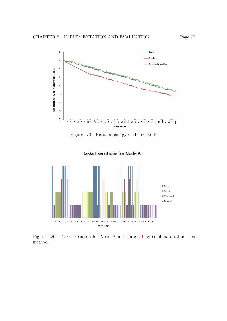
CHAPTER 5. IMPLEMENTATION AND EVALUATION Page 72
Figure 5.19: Residual energy of the network.
Figure 5.20: Tasks execution for Node A in Figure 4.1 by combinatorial auctionmethod.

CHAPTER 5. IMPLEMENTATION AND EVALUATION Page 73
Figure 5.21: Tasks execution for Node B in Figure 4.1 by combinatorial auctionmethod.
Figure 5.22: Tasks execution for Node C in Figure 4.1 by combinatorial auctionmethod.

CHAPTER 5. IMPLEMENTATION AND EVALUATION Page 74
Figure 5.23: Cumulative revenue of the network with three agents.
5.4 Comparison of RL, CRL, and Exp3
We perform the evaluation of RL, CRL, and Exp3 considering the system modeldescribed in the Subsection 3.2.1. For our evaluation we perform the following fiveexperiments with the following assumptions of parameters.
1. To find out the trade-off between tracking quality and energy consumption,we set the balancing factor β of the reward function between [0.1,0.9] in 0.1steps, keep the randomness of moving targets as η = 0.5, set the egalitarianismfactor of Exp3 as κ = 0.5 and fix the topology to five nodes.
2. We vary the network size to check the trade-off between tracking quality andenergy consumption. We consider three different topologies consisting of 5, 10,and 20 sensor nodes where the coverage ratio is 0.0029, 0.0057, and 0.0113,respectively. The coverage ratio is defined as the ratio of the aggregated FOVof all deployed sensor nodes over the area of the entire surveillance area. Wekeep the balancing factor β = 0.5 and the randomness of the mobility modelη = 0.5 constant for this experiment.
3. We set the randomness of moving targets η to one of the following values{0.1, 0.15, 0.2, 0.25, 0.3, 0.4, 0.5, 0.7, 0.9} and set the balancing factor β = 0.5and fix the topology to five nodes.
4. We vary the sensing range r to one of these values {10,15,20,25,30,35,40,45}for this experiment.
5. We evaluate RL, CRL, and Exp3 in terms of average execution time and aver-age communication effort. These values are measured from twenty iterationsand represent the mean execution times and the mean of Send Message taskexecutions.

CHAPTER 5. IMPLEMENTATION AND EVALUATION Page 75
Figure 5.24 shows the tracking quality/energy consumption trade-off for RL,CRL, and Exp3 by varying the balancing factor, β between [0.1,0.9] in 0.1 steps.Table 5.2 shows the evaluation of RL, CRL, and Exp3 based on tracking quality,energy consumption, and average communication effort varying the balancing factorβ. Each data point in these figures represents the average of normalized trackingquality and energy consumption of ten complete simulation runs. We observe thatCRL and Exp3 provide similar results, i.e., the corresponding data points are closelyco-located. RL is more energy aware but is not able to achieve high tracking quality.
Figure 5.25 shows the tracking-quality/energy consumption trade-off varying thenumber of nodes to 5, 10, and 20. Table 5.3 shows the mean and variance values ofthe tracking quality and energy consumption for the RL, CRL, and Exp3 varyingthe number of nodes, N . In this experiment, each data point represents the averageof normalized tracking quality and energy consumption of ten complete simulationruns. Here the same trend can be identified, i.e., the CRL and Exp3 achieve almostsimilar results in terms of tracking quality/energy consumption trade-off and RLshows less tracking performance with higher energy efficiency.
Figures 5.26, 5.27, and 5.28 show the results by varying η to one of these values{0.1,0.15,0.2,0.25,0.3,0.4,0.5,0.7, and 0.9}. Each data point in these figures repre-sents the average of normalized tracking quality and energy consumption of tencomplete simulation runs. From these figures, it can be seen that CRL and Exp3outperform RL in terms of achieved tracking performance. We can see that forlower randomness, η=0.5, 0.7, and 0.9, RL and Exp3 show very close results fortracking performance. But for higher randomness, η= 0.1, 0.15, and 0.2, RL givespoor performance with regard to tracking performance.
Figure 5.29 shows the results of tracking quality/energy consumption trade-offof RL, CRL, and Exp3 for different coverage ratio. The coverage ratio is definedas the ratio of the aggregated FOV of all deployed sensor nodes As over the areaof the entire surveillance area An. Here, each data point represents average of thenormalized tracking quality and energy consumption of ten complete simulationruns. We can observe that higher the As/An ratio, less the tracking quality. HigherAs/An means more spaces are not covered by the considered sensor nodes and thesensing radius r of each sensor node is smaller. We vary r to one of these values{10,15,20,25,30,35,40,45} for this experiment. The surveillance area is a rectanglewith the height of 300 unit and width of 460 unit. Area of a particular node isconsidered as πr2. As is the surveillance area considered as (height×width). Fromthe figure, it can be seen that Exp3 outperforms the RL in terms of tracking quality.CRL shows higher tracking quality but poor performance with regard to energyconsumption.
Table 5.4 shows the comparison of RL, CRL, and Exp3 in terms of average exe-cution time and average communication effort. These values are derived from twentyiterations and represent the mean execution times and the mean of Send messagetask executions. We find that RL is the most resource-aware scheduling algorithm.Exp3 requires 25% more and CRL requires 86% more execution time, respectively.

CHAPTER 5. IMPLEMENTATION AND EVALUATION Page 76
The communication overhead is similar for both Exp3 and CRL.
Figure 5.24: Tracking quality/energy consumption trade-off for RL, CRL, and Exp3by varying the balancing factor of the reward function β.
RL CRL Exp3TQ EC ACE TQ EC ACE TQ EC ACE
β=0.1 0.43 3.90 0 0.49 4.00 21 0.48 3.96 18β=0.2 0.45 3.92 0 0.51 4.20 23 0.50 4.10 20β=0.3 0.48 3.99 0 0.52 4.33 26 0.52 4.20 23β=0.4 0.50 4.18 0 0.54 4.59 28 0.53 4.39 25β=0.5 0.52 4.23 0 0.55 4.65 30 0.54 4.52 28β=0.6 0.53 4.53 0 0.59 4.69 32 0.57 4.61 30β=0.7 0.54 4.67 0 0.64 4.97 33 0.64 4.89 32β=0.8 0.62 4.99 0 0.68 6.00 35 0.67 5.89 34β=0.9 0.74 5.19 0 0.77 6.50 37 0.76 6.39 36
Table 5.2: Comparison of RL, CRL, and Exp3 based on Tracking Quality (TQ),Energy Consumption (EC), and Average Communication Effort (ACE) by varyingthe balancing factor of the reward function β.

CHAPTER 5. IMPLEMENTATION AND EVALUATION Page 77
Figure 5.25: Tracking quality/energy consumption trade-off for RL, CRL, and Exp3by varying the network size.
RL CRL Exp3TQ EC TQ EC TQ EC
Mean (N=5) 0.51 4.10 0.54 5.20 0.54 4.45Variance (N=5) 0.0016 0.26 0.0012 0.23 0.0011 0.21Mean (N=10) 0.69 5.10 0.78 6.01 0.78 5.49
Variance (N=10) 0.0016 0.26 0.0012 0.23 0.0011 0.21Mean (N=20) 0.81 6.49 0.87 6.99 0.85 6.75
Variance (N=20) 0.0014 0.09 0.0013 0.07 0.0010 0.07
Table 5.3: Mean and variance of the tracking quality and the energy consumptionby varying the number of nodes, N=5, 10, and 20. Here TQ means Tracking Qualityand EC means Energy Consumption.

CHAPTER 5. IMPLEMENTATION AND EVALUATION Page 78
Figure 5.26: Tracking quality/energy consumption trade-off for RL, CRL, and Exp3by varying the randomness of target movement, η = 0.10, 0.15, and 0.20.
Figure 5.27: Tracking quality/energy consumption trade-off for RL, CRL, and Exp3by varying the randomness of target movement, η = 0.25, 0.30, and 0.40.

CHAPTER 5. IMPLEMENTATION AND EVALUATION Page 79
Figure 5.28: Tracking quality/energy consumption trade-off for RL, CRL, and Exp3by varying the randomness of target movement, η = 0.50, 0.70, and 0.90.
Figure 5.29: Results varying the sensing radius

CHAPTER 5. IMPLEMENTATION AND EVALUATION Page 80
Avg. Execution Time Avg. Comm. EffortRL 0.036 s 0
CRL 0.067 s 29Exp3 0.045 s 27
Table 5.4: Comparison of average execution time and average number of transferredmessages (based on 20 iterations).
5.5 Discussion
All above results help us to reach the following decisions.
• Cooperative task scheduling methods (CRL (one hop and two hop), Coopera-tive Q learning, Exp3) provide better performance, e.g., tracking quality thannon-cooperative or independent task scheduling method (RL).
• Cooperative approaches require more resources, e.g., energy due to the increasecommunication effort.
• By appropriately setting the balancing factor of the reward function β thedesired performance or energy consumption can be achieved.
• Further cooperation among neighboring nodes with the local observationshelp to achieve better performance. CRL(two hop) outperforms the RL andCRL(one hop) in terms of tracking quality.
• Online task scheduling methods outperform the offline task scheduling meth-ods in terms of remaining energy of the network.
• Our evaluation shows that different methods have different properties con-cerning resource-awareness and achieved performance. The selection of thescheduling algorithm thus depends on the application requirements and avail-able resources of the WSN.

CHAPTER
6Conclusion and future work
Resource-aware effective task scheduling is very important for WSN to know thebest task to execute on next time slots. We propose two cooperative reinforcementlearning methods (cooperative Q learning and SARSA(λ)), bandit solvers (Exp3),and market based method for online scheduling of tasks in a way that the bet-ter energy/performance trade-off is achieved. We perform the evaluation of ourproposed cooperative methods (one hop and two hop distance neighbors) and non-cooperative method. Our experimental results show that our cooperative schedulingoutperforms the non-cooperative scheduling in terms of tracking quality. We showthat cooperation among neighboring nodes improves the energy/performance trade-off comparing with the non-cooperative approach. We also perform the evaluationof RL, CRL, and Exp3. We apply our methods in a target tracking application. Wefind that RL, CRL, and Exp3 have different properties based on tracking qualityand energy efficiency. The selection of a particular scheduling algorithm depends onthe requirement of the application and available resources of sensor nodes.
6.1 Summary of contributions
We propose cooperative Q learning for task scheduling in a WSN. This is our firstinitiative to apply a reinforcement learning method for task scheduling. We assume aset of tasks and a set of states for applying Q learning. To our best knowledge, this isthe first work to consider some cooperation among neighbors for task scheduling in aWSN. We consider static values for the reward of the performed actions. We providehigher reward values for the tasks which consume less energy for the execution. Weapply this method in a target tracking application and compare with static, randomand existing individual reinforcement learning method. We consider only three nodeswith a particular movement of a target. We consider two application scenarios withtwo sets of reward values. We calculate the cumulative reward over time for allmethods. We find task execution at each time step considering three sensor nodes.We calculate the total number of executions for each action and also the residual
81

CHAPTER 6. CONCLUSION AND FUTURE WORK Page 82
energy of the network over time. We find that our proposed cooperative learningoutperforms the existing approaches in terms of energy efficiency.
We propose a combinatorial auction-based method for task scheduling in a WSN.We have a set of tasks. Each task requires CPU cycle, energy requirements, and idealsleep time for execution. We calculate the variance of the available energy of thesensor nodes. The higher variance value corresponds to the unbalanced availableenergy among the sensor nodes which is not energy efficient. We calculate theresidual energy of the network and perform the evaluation of our proposed approachwith the existing static and random task scheduling. We find out the task executionfor each considered node over time steps. We also calculate the revenue of thenetwork by a simulator. We observe that our proposed approach outperforms interms of energy efficiency and task scheduling comparing with static and randomtask scheduling.
We propose a cooperative SARSA(λ) learning algorithm for task scheduling ina WSN. For this work, we update our state and action space with the trajectoryprediction action and the awareness state. We consider a weighted reward functionto trade the application performance and energy consumption. We perform theexperiments to find out the trade-off between application performance and resourceconsumption by varying the balancing factor of the reward function. We also varythe randomness of the target movement and the number of nodes to identify theperformance/resource consumption trade-off. We observe that proposed cooperativeapproach outperforms the non-cooperative approach in terms of tracking quality.
We propose an exponential bandit solvers Exp3 for task scheduling in WSN.We perform the evaluation of Exp3 with RL and CRL. We find the tracking qual-ity/energy consumption trade-off for methods. We observe that Exp3 and CRLprovide close results in terms of tracking quality/energy consumption trade-off. RLprovides the most energy efficiency but less tracking quality. We also calculatethe average execution time and communication overhead for these methods. Herewe find that CRL and Exp3 provide close results in terms of execution time andcommunication overhead.
We observe that cooperation among neighboring nodes helps to achieve betterperformance. Cooperative task scheduling methods outperform the non-cooperativeor independent task scheduling methods in terms of tracking quality. Independentscheduling methods provide better energy efficiency compared with cooperative taskscheduling as there is no message exchange for the cooperation in independent learn-ing methods. Online task scheduling methods help to learn the best next task toexecute based on past observed application behavior. We find that our proposedmethods have different properties based on resource-awareness and achieved perfor-mance. The selection of the appropriate method depends on the application demandand the remaining resources of the WSN.

CHAPTER 6. CONCLUSION AND FUTURE WORK Page 83
6.2 Future works
This thesis opens up so many issues based on resource-aware task scheduling inWSNs. To find suitable methods for better application performance with optimizedresource consumption is one of the challenges. Future work includes the applicationof our resource-aware scheduling approach to different WSN applications, the im-plementation on our visual sensor network platforms [24] and the comparison of ourapproach with other variants of reinforcement learning methods.
Currently we are using our task scheduling methods for a multi-target trackingapplication. There are some other applications, e.g., routing protocols, mediumaccess control (MAC) protocols, etc. There are some existing works of RL-basedrouting protocol design to find optimal routing paths [22] [25] [83]. There are someexisting RL-based MAC protocols [15] [56]. One of our future works is to apply ourproposed CRL for the routing protocol and MAC protocol design.
We have a plan to apply our proposed task scheduling methods on our visual sen-sor network platforms [24]. Currently we are considering sensor nodes with limitedenergy supply in a rectangular area for moving target tracking application.
We plan to compare our proposed RL method with the other variants of RL.Currently we are using cooperative Q and SARSA(λ) learning. There are someother variants of RL like Q(λ), temporal difference (TD), TD(λ) and SARSA [80].We plan to evaluate our proposed methods with Q(λ), TD, TD(λ), and SARSA.

Bibliography
[1] T. Abbes, S. Mohamed, and K. Bouabdellah. Impact of Model Mobility in AdHoc Routing Protocols. Computer Network and Information Security, 10:47–54,2012.
[2] K. Akkaya and M. Younis. A survey of routing protocols in wireless sensornetworks. Ad Hoc Network (Elsevier), 3(3):325–349, 2005.
[3] I. F. Akyildiz, T. Melodia, and K. R. Chowdhury. A survey on wireless multi-media sensor networks. Computer Networks, 51:921–960, 2007.
[4] I. F. Akyildiz, W. Su, Y. Sankarasubramaniam, and E. Cayirci. Wireless sensornetworks: a survey. Elsevier Computer Networks, 38:393–422, 2002.
[5] T. Arampatzis, J. Lygeros, and S. Manesis. A survey of applications of wire-less sensors and wireless sensor networks. In Proceedings of IEEE MediterreanConference on Control and Automation, pages 719–724, 2005.
[6] P. Auer, N. C. Bianchi, Y. Freund, and R. E. Schapire. The nonstochasticmultiarmed bandit problem. SIAM Journal on Computing, 32:48–77, 2002.
[7] S. Ben-david, E. Kushilevitz, and Y. Mansour. Online learning versus offlinelearning. Computational Learning Theory, 904:38–52, 1995.
[8] N. Bery. Linear regression. Technical report, DataGenetics, 2009.
[9] A. Bharathidasan, V. Anand, and S. Ponduru. Sensor networks: An overview.In IEEE Potentials, volume 22, pages 20–23, 2003.
[10] A. Blum. On-line algorithms in machine learning. In Proceedings of the Work-shop on On-Line Algorithms, pages 306–325, 1996.
[11] O. Boyinbode, H. Le, A. Mbogho, M. Takizawa, and R. Poliah. A survey onclustering algorithms for wireless sensor networks. In International Conferenceon Network-Based Information Systems, pages 358–364, 2010.
[12] M. Bramwell. Implementing a mica2 mote sensor network. Technical report,Crossbow-Mica2 Mote, 2006.
84

BIBLIOGRAPHY Page 85
[13] J. Byers and G. Nasser. Utility Based Decision making in Wireless SensorNetworks. In Proceedings of the Workshop on Mobile and Ad Hoc Networkingand Computing, pages 143 – 144, 2000.
[14] L. Chen, B. K. Szymanski, and J. W. Branch. Auction-based congestion man-agement for target tracking in wireless sensor networks. In Proceedings of theIEEE International Conference on Pervasive Computing and Communications,pages 1–10, 2011.
[15] Y. Chu, P. Mitchell, and D. Grace. Aloha and q-learning based medium accesscontrol for wireless sensor networks. In International Symposium on WirelessCommunication Systems, pages 511–515, 2012.
[16] B. Coltin and M. Veloso. Mobile robot task allocation in hybrid wireless sensornetworks. In Proceedings on IEEE/RSJ International Conference on IntelligentRobots and Systems (IROS), pages 2932–2937, 2010.
[17] D. Culler, D. Estrin, and M. Srivastava. Overview of sensor networks. IEEEComputer Society, pages 41–49, 2004.
[18] W. Dargie and C. Poellabauer. Fundamentals of Wireless Sensor Networks.Wiley, 2010.
[19] R. Dechter and D. Frost. Backtracking algorithms for constraint satisfactionproblems. Technical report, University of California, Irvine, 1999.
[20] S. Denef, L. Ramirez, and T. Dyrks. Letting tools talk: Interactive technol-ogy for firefighting. In Proceedings of ACM Conference on Human Factors inComputing Systems, pages 4447–4452, 2009.
[21] S. Dhanani, J. Arseneau, A. Weatherton, B. Caswell, N. Singh, and S. Patek.A comparison of utility based information management policies in sensor net-works. In Systems Technology Integration Lab of the Department of Systemsand Information Engineering at the University of Virginia, Charlottesville, VA.,pages 84–89, 2006.
[22] S. Dong, P. Agrawal, and K. Sivalingam. Reinforcement learning based ge-ographic routing protocol for uwb wireless sensor network. In IEEE GlobalTelecommunications Conference, pages 652–656, 2007.
[23] N. Edalat, W. Xiao, N. Roy, S. Das, and M. Motani. Combinatorial auctionbased task allocation in multi application wireless sensor networks. In Proceed-ings of the international conference on Embedded and Ubiquitous Computing,pages 174–181, 2011.

BIBLIOGRAPHY Page 86
[24] L. Esterle, P. R. Lewis, X. Yao, and B. Rinner. Socio-Economic Vision GraphGeneration and Handover in Distributed Smart Camera Networks. ACM Trans-actions on Sensor Networks, 10(2):24, 2014.
[25] A. Forster and A. Murphy. Froms: Feedback routing for optimizing multiplesinks in wsn with reinforcement learning. In IEEE International Conference onIntelligent Sensors, Sensor Networks and Information, pages 371–376, 2007.
[26] C. Frank and K. Romer. Algorithms for Generic Role Assignments in Wire-less Sensor Networks. In Proceedings of the ACM Conference on EmbeddedNetworked Sensor Systems, pages 230–242, 2005.
[27] A. Galstyan. Resource allocation and emergent coordination in wireless sensornetworks. In Workshop on Sensor Networks at the The Nineteenth NationalConference on Artificial Intelligence (AAAI-04), pages 1–6, 2004.
[28] Z. Ghahramani. Unsupervised learning. In Advanced Lectures on MachineLearning, pages 72–112. Springer-Verlag, 2004.
[29] S. Giannecchini, M. Caccamo, and C. Shih. Collaborative Resource Allocationin Wireless Sensor Networks. In Proceedings of the Euromicro Conference onReal-Time Systems, pages 35–44, 2004.
[30] A. Goldsmith and S. Wicker. Design challenges for energy-constrained ad hocwireless networks. IEEE Wireless Communications Magazine, 9:8–27, 2002.
[31] W. Guo, N. Xiong, H.-C. Chao, S. Hussain, and G. Chen. Design and Analysisof Self Adapted Task Scheduling Strategies in WSN. Sensors, 11:6533–6554,2011.
[32] A. Hac. Wireless Sensor Network Designs. John Wiley and Sons, 2003.
[33] V. Handziski, A. Kopk, H. Karl, and A. Wolisz. A common wireless sensornetwork architecture? Technical report, Technical University of Berlin, 2003.
[34] W. R. Heinzelman, J. Kulik, and H. Balakrishnan. Adaptive protocols for infor-mation dissemination in wireless sensor networks. In Proceedings of the AnnualACM/IEEE International Conference on Mobile Computing and Networking,pages 174–185, 1999.
[35] J. Huang, Z. Han, M. Chiang, and H. V. Poor. Auction-based resource al-location for cooperative communications. IEEE Journal on Selected Areas inCommunications, pages 1226–1237, 2008.
[36] M. M. Islam, M. M. Hassan, G. W. Lee, and E. N. Huh. A survey on virtual-ization of wireless sensor networks. Sensors, 12(2):2175–2207, 2012.

BIBLIOGRAPHY Page 87
[37] D. Jea and M. B. Srivastava. Channels characteristics for on-body mica2dotwireless sensor networks. Technical report, Networked and Embedded SystemsLaboratory, University of California, Los Angeles, 2003.
[38] L. P. Kaelbling, M. L. Littman, and A. W. Moore. Reinforcement learning: asurvey. Journal of Artificial Intelligence Research, 4:237–285, 1996.
[39] J. M. Kahn, R. H. Katz, and K. S. J. Pister. Emerging challenges: Mobilenetworking for smart dust. Journal of Communications and Networks, 2(3),2000.
[40] A. E. Kateeb, A. Ramesh, and L. Azzawi. Wireless sensor nodes processorarchitecture and design. In Canadian Conference on Electrical and ComputerEngineering, pages 1031–1034, 2008.
[41] M. I. Khan and B. Rinner. Resource Coordination in Wireless Sensor Networksby Cooperative Reinforcement Learning. In Proceedings of the IEEE Interna-tional Conference on Pervasive Computing and Communications Workshops,pages 895 – 900, 2012.
[42] M. I. Khan and B. Rinner. Energy-Aware Task Scheduling in Wireless SensorNetworks by Cooperative Reinforcement Learning. In Proceedings of the IEEEInternational Conference on Communications Workshops, pages 871–877, 2014.
[43] M. I. Khan and B. Rinner. Evaluation of Resource-Aware Task SchedulingMethods in Wireless Sensor Networks. IEEE Sensor Journal, page 2, 2014.
[44] M. I. Khan and B. Rinner. Performance Analysis of Resource-Aware TaskScheduling Methods in Wireless Sensor Networks. Hindawi International Jour-nal of Distributed Sensor Networks, page 9, 2014.
[45] M. I. Khan, B. Rinner, and C. S. Regazzoni. Resource Coordination in WirelessSensor Networks by Combinatorial Auction Based Method. In Proceedings ofthe IEEE International Conference on Networked Embedded Systems for EveryApplications, pages 1–6, 2012.
[46] U. A. Khan and B. Rinner. Online Learning of Timeout Policies for DynamicPower Management. ACM Transactions on Embedded Computing Systems,page 25, 2013.
[47] C. Kim and J. Ahn. Causally ordered delivery protocol for overlapping multicastgroups in broker-based sensor networks. International Journal of ComputerScience Issues, Vol 8, Issue 1, pages 46–54, 2011.
[48] L. Kleinrock. Distributed systems. Communications of the ACM, 28(11), 1985.

BIBLIOGRAPHY Page 88
[49] P. Klemperer. Auction theory: A guide to the literature. Journal of EconomicSurveys, 13(3):227–286, 1999.
[50] J. Ko, K. Klues, C. Richter, M. B. Wanja Hofer, Branislav Kusy, T. Schmid,Q. Wang, P. Dutta, and A. Terzis. Low Power or High Performance? A Trade-off Whose Time Has Come (and Nearly Gone). In Proceedings of EuropeanConference on Wireless Sensor Networks, pages 98–114, 2012.
[51] S. Kogekar, E. Neema, O. Eames, X. Koutsoukos, A. Ledeczi, and M. Maroti.Constraint-guided dynamic reconfiguration in sensor networks. In Informationprocessing in sensor networks, pages 379–387. ACM Press, 2004.
[52] H. Kopetz. Real-Time Systems - Design Principles for Distributed EmbeddedApplications. Springer, 2011.
[53] B. Krishnamachari and S. Wicker. On the complexity of distributed self-configuration in wireless networks. Journal of Telecommunication Systems,pages 33–59, 2003.
[54] J. E. Lee, S. H. Cha, D. Y. Kim, and K. H. Cho. Autonomous management oflarge-scale ubiquitous sensor networks. Emerging Directions in Embedded andUbiquitous Computing, pages 609–618, 2006.
[55] T. Liu and M. Martonosi. Impala: A middleware system for managing auto-nomic, parallel sensor systems. In Proceedings of the ninth ACM SIGPLANsymposium on Principles and practice of parallel programming, pages 107–118.ACM Press, 2003.
[56] Z. Liu and I. Elhanany. Rl-mac: A reinforcement learning based mac pro-tocol for wireless sensor networks. International Journal of Sensor Networks,1(3):117–124, 2006.
[57] T. A. Malik. Target Tracking in Wireless Sensor Networks. PhD thesis, Ma-harshi Dayanand University, 2003.
[58] D. C. Montgomery, E. A. Peck, and G. G. Vining. Introduction to LinearRegression Analysis. Wiley, 2007.
[59] J. F. Nash. Equilibrium points in n-person games. In Proceedings of the NationalAcademy of Sciences of the United States of America, volume 36, pages 48–49,1950.
[60] H. Park and M. B. Srivastava. Energy-efcient task assignment framework forwireless sensor networks. Technical report, University of California, Los Ange-les, 2012.

BIBLIOGRAPHY Page 89
[61] M. A. Perillo and W. B. Heinzelman. Wireless sensor network protocols. Tech-nical report, University of Rochester, 2005.
[62] C. S. Raghavendra, K. M. Sivalingam, and T. Znati. Wireless Sensor Networks.Springer, 2006.
[63] M. L. Rasneet Kaur. Wireless Sensor Networks: A Survey. International Jour-nal of Electronics and Communication Technology, 4(3):102–106, 2013.
[64] Z. Ruyan, L. Huifang, H. Shijun, and W. Dongyun. Data processing and nodemanagement in wireless sensor network. In International Symposium on Com-puter Network and Multimedia Technology, pages 1–4, 2009.
[65] M. G. Sandra Sendra, Jaime Lloret and J. F. Toledo. Power saving and energyoptimization techniques for wireless sensor networks. Journal of communica-tions, 6:439–459, 2011.
[66] K. Shah and M. Kumar. Distributed Independent Reinforcement Learning(DIRL) Approach to Resource Management in Wireless Sensor Networks. InProceedings of IEEE Mobile Adhoc and Sensor Systems, pages 1–9, 2007.
[67] K. Shah and M. Kumar. Resource Management in Wireless Sensor NetworksUsing Collective Intelligence. In Proceedings of Intelligent Sensors, Sensor Net-works and Information Processing, pages 423–428, 2008.
[68] J. Shanbehzadeh, S. Mehrjoo, and A. Sarrafzadeh. An intelligent energy effi-cient clustering in wireless sensor networks. In Proceedings of the internationalmulticonference of engineers and computer scientists, volume 1, pages 1–5, 2011.
[69] E. Shih, P. Bahl, and M. J. Sinclair. Wake on wireless: an event driven energysaving strategy for battery operated devices. In Proceedings of the 8th AnnualInternational Conference on Mobile Computing and Networking, pages 160–171,2002.
[70] H. Shih, X. Zhang, D. S. L. Wei, K. Naik, and R. C. Chen. Design and im-plementation of a mobile sensor network testbed using sun spots. Journal ofFuture Computer and Communication, 2(2):115–120, 2013.
[71] S. S. Shwartz. Online Learning: Theory, Algorithms, and Applications. PhDthesis, Senate of the Hebrew University, 2007.
[72] A. Silberschatz, G. Gagne, and P. Galvin. Operating system concepts. Addison-Wesley, 2008.
[73] P. Sivaram and S. Angadi. Wireless sensor networks: Routing protocols, chal-lenges, solutions. Interantional Journal of P2P Network Trends and Technology(IJPTT), 3(4):214–217, 2013.

BIBLIOGRAPHY Page 90
[74] K. Sohraby, D. Minoli, and T. Znati. Wireless Sensor Networks: Technology,Protocols, and Applications. Wiley, 2007.
[75] E. Soulas and D. Shasha. Online machine learning algorithms for currencyexchange prediction. Technical report, NYU CS Technical Report TR-2013-953, 2013.
[76] M. Spiegel. Theory and Problems of Probability and Statistics. McGraw-Hill,1992.
[77] W. Stallings. Operating Systems. Pearson Education, 2006.
[78] D. J. Stein. Wireless sensor network simulator v1.0, March 2005.
[79] I. Stojmenovic. Handbook of Sensor Networks, Algorithms and Architectures.Wiley, 2010.
[80] R. S. Sutton and A. G. Barto. Reinforcement Learning: An Introduction. MITPress, 1998.
[81] Y. Tian, E. Ekici, and F. Ozguner. Energy-constrained Task Mapping andScheduling in Wireless Sensor Networks. In Proceedings of the IEEE Inter-national Conference on Mobile Adhoc and Sensor Systems Conference, pages210–218, 2005.
[82] N. Tsiftes, A. Dunkels, Z. He, and T. Voigt. Enabling large scale storage insensor networks with coffee file system. In International Conference on Infor-mation Processing in Sensor Networks, pages 349–360, 2009.
[83] R. A. Valles, R. A. Rodriguez, A. G. Curieses, and J. C. Sueiro. Q-probabilisticrouting in wireless sensor networks. In IEEE International Conference on In-telligent Sensors, Sensor Networks and Information, pages 1–6, 2007.
[84] J. M. Vidal. Multiagent coordination using a distributed combinatorial auc-tion. In Proceedings of the AAAI Workshop on Auction Mechanisms for RobotCoordination, pages 1–7, 2006.
[85] C. Watkins and P. Dayan. Q-Learning. Machine Learning, pages 279–292,1992.
[86] M. Weiser, B. Welch, A. Demers, and S. Shenker. Scheduling for reduced cpuenergy. In USENIX Conference on Operating Systems Design and Implemen-tation, pages 13–23, 1994.
[87] U. Wilensky. NetLogo. Technical report, Center for connected learning andcomputer based modeling, Northwestern University, Evanston, IL, 1999.

BIBLIOGRAPHY Page 91
[88] F. Yao, A. Demers, and S. Shenker. A scheduling model for reduced cpu energy.In Annual Symposium on Foundations of Computer Science, pages 374–382,1995.
[89] K. L. A. Yau, P. Komisarczuk, and P. D. Teal. Reinforcement Learning for Con-text Awareness and Intelligence in Wireless Networks: Review, New Featuresand Open Issues. Journal of Network and Computer Applications, 35:253–267,2012.
[90] J. Yick, B. Mukherjee, and D. Ghosal. Wireless sensor network survey. Journalof Computer Networks, 52(12):2292–2330, 2008.
[91] E. Yoneki and J. Bacon. A survey of wireless sensor network technologies:research trends and middleware’s role. Technical Report UCAM-CL-TR-646,University of Cambridge, Computer Laboratory, Sept. 2005.