Reservoir-System Model for the

Willamette River Basin,

Oregon

By James 0. Shearman

RIVER-QUALITY ASSESSMENT OF THE WILLAMETTE RIVER BASIN, OREGON

GEOLOGICAL SURVEY CIRCULAR 715-H

1976

United States Department of the Interior

THOMAS S. KLEPPE, Secretary

Geological Survey V. E. McKelvey, Director

Library of Congress Cataloging in Publication Data

Shearman, James 0. Reservoir-system model for the Willamette River Basin, Oregon. (River-quality assessment of the Willamette River Basin, Oregon)

(U.S. Geological Survey Circular 715-H) Bibliography: p. 22. 1. Willamette River watershed. 2. Stream measurements-Mathematical models. 3. Stream

measurements-Data processing. 4. Reservoirs-Mathematical models. 5. Reservoirs-Data processing. I. Title. II. Series. III. Series: United States Geological Survey Circular 715-H.

QE75.CS no. 715-H[GB1225.07] 557.3'08s [627'.86'097953] 76-608239

Free on application to Branch of Distribution, U.S. Geological Survey, 12 0 0 South Eads Street, Arlington, VA 2 2 2 o 2

FOREWORD

The American public has identified the enhancement and protection of river quality as an important national goal, and recent laws have given this commit­ment considerable force. As a consequence, a considerable investment has been made in the past few years to improve the quality of the Nation's rivers. Further improvements will require substantial expenditures and the consumption of large amounts of energy. For these reasons, it is important that alternative plans for river-quality management be scientifically assessed in terms of their relative ability to produce environmental benefits. To aid this endeavor, this circular series presents a case history of an intensive river-quality assessment in the Willamette River basin, Oregon.

The series examines approaches to and results of critical aspects of river­quality assessment. The first several circulars describe approaches for providing technically sound, timely information for river-basin planning and manage­ment. Specific topics include practical approaches to mathematical modeling, analysis of river hydrology, analysis of earth resources-river quality relations, and development of data-collection programs for assessing specific problems. The later circulars describe the application of approaches to existing or potential river-quality problems in the Willamette River basin. Specific topics include maintenance of high-level dissolved oxygen in the river, effects of reservoir release patterns on downstream river quality, algal growth potential, distribu­tion of toxic metals, and the significance of erosion potential to proposed future land and water uses.

Each circular is the product of a study devoted to developing resource informa­tion for general use. The circulars are written to be informative and useful to informed laymen, resource planners, and resource scientists. This design stems from the recognition that the ultimate success of river-quality assessment depends on the clarity and utility of approaches and results as well as their basic scientific validity.

Individual circulars will be published in an alphabetical sequence in the Geological Survey Circular 715 series entitled ~(River-Quality Assessment of the Willamette River Basin, Oregon."

J. S. Cragwall, Jr. Chief Hydrologist

III

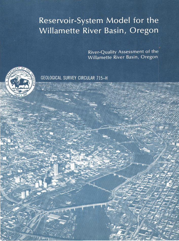
Cover: Willamette River as it winds through Portland, Oregon. Photograph taken by

Hugh Ackroyd.

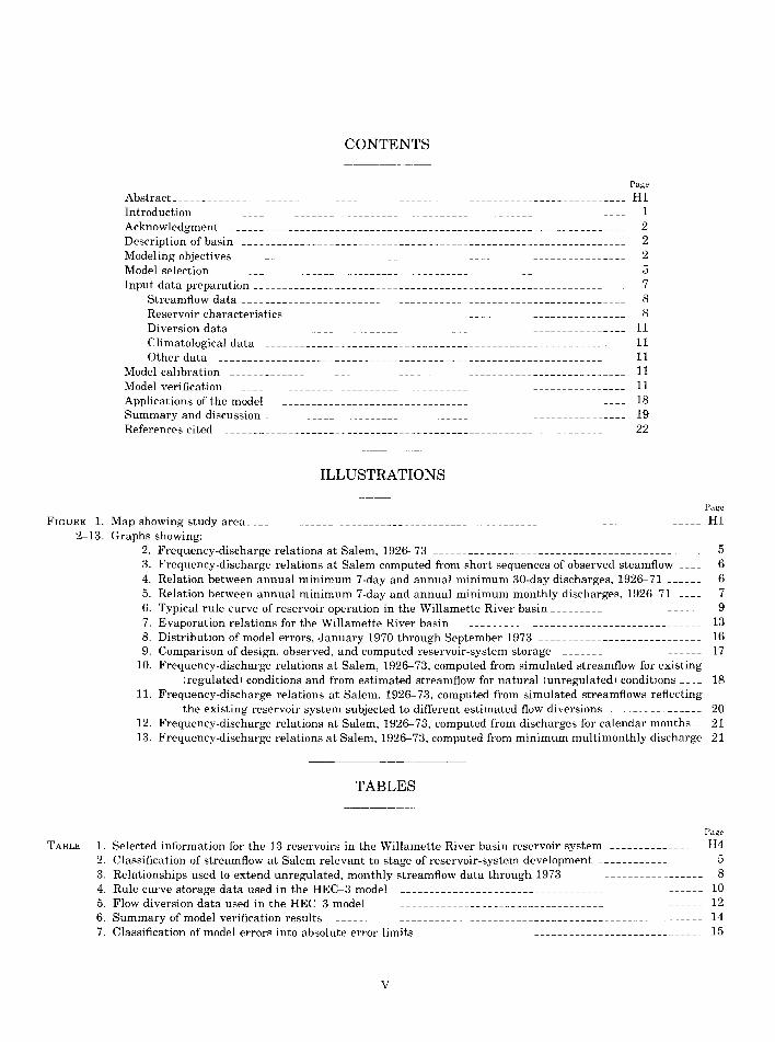
CONTENTS

Page 1\bstract ______________________________________________________________________________ Ill

Introduction-------------------------------------------------------------------------- 1 1\cknovvledgment -------------------------------------------------------------------- 2 Description of basin __ __ _ ___ _ _ __ __ __ _ _ _ ___ _ _ _ _ ____ _ _ _ _ __ __ __ _ _ __ __ _ _ __ ____ _ _ ____ __ _ _ _ _ 2

~odeling objectives ------------------------------------------------------------------ 2 ~odel selection ---------------------------------------------------------------------- 5 Input data preparation---------------------------------------------------------------- 7

Strea~ftovv data------------------------------------------------------------------ 8 Reservoir characteristics ---------------------------------------------------------- 8 Diversion data____________________________________________________________________ 11 Climatological data _ _ _ _ __ __ _ _ __ _ _ _ _ _ ___ __ _ _ __ _ ___ _ ___ __ _ _ _ _ _ _ __ _ _ ____ __ _ _ _ _ _ _ _ _ __ 11

Other data ---------------------------------------------------------------------- 11 ~odel calibration _ _ ___ ___ _ _ ______ _ _ _ _ ___ _ _____ ___ _ _ ____ _ _ _ _ _ _ __ _ _ _ _ ___ _ _ _ _ _ __ _ _ _ _ __ __ 11 ~odel verification __ _ _ _ _ __ _ _ _ ___ __ __ _ _ ____ _ _ _____ _ _ _ ______ __ _ _ __ __ _ _ _ __ _ __ ____ _ _ _ _ __ __ 11 1\pplications of the model______________________________________________________________ 18

Summary and discussion -------------------------------------------------------------- 19 References cited ---------------------------------------------~------------------------ 22

ILLUSTRATIONS

Page

FIGURE 1. ~ap shovving study area______________________________________________________________________________ Ill 2-13. Graphs shovving:

2. Frequency-discharge relations at Salem, 1926-73 _________ ______________ ______________ _________ 5 3. Frequency-discharge relations at Salem computed from short sequences of observed steamflovv ____ 6 4. Relation betvveen annual minimu~ 7-day and annual minimu~ 30-day discharges, 1926-71 ______ 6 5. Relation betvveen annual minimum 7-day and annual minimu~ monthly discharges, 1926-71 ____ 7 6. Typical rule curve of reservoir operation in the Willamette River basin-------------------------- 9 7. Evaporation relations for the Willamette River basin ------------------------------------------ 13 8. Distribution of model errors, January 1970 through September 1973 ---------------------------- 16 9. Comparison of design, observed, and computed reservoir-system storage ------------------------ 17

10. Frequency-discharge relations at Salem, 1926-73, computed from simulated streamftovv for existing (regulated) conditions and from estimated streamftovv for natural (unregulated! conditions ____ 18

11. Frequency-discharge relations at Salem, 1926-73, co~puted from simulated streamftovvs reflecting the existing reservoir system subjected to different estimated ftovv diversions ---------------- 20

12. Frequency-discharge relations at Salem, 1926-73, computed from discharges for calendar months__ 21 13. Frequency-discharge relations at Salem, 1926-73, co~puted from minimum multimonthly discharge 21

TABLES

Page

TABLE 1. Selected information for the 13 reservoirs in the Willamette River basin reservoir system ---------------- II4 2. Classification of streamftovv at Salem relevant to stage of reservoir-system development ------------------ 5 3. Relationships used to extend unregulated, monthly streamftovv data through 1973------------------------ 8 4. Rule curve storage data used in the IIEC-3 ~odeL _____________________________________________________ 10

5. Flovv diversion data used in the IIEC-3 model -------------------------------------------------------- 12 6. Summary of model verification results __________________________________________________________ ------ 14

7. Classification of model errors into absolute error limits ------------------------------------------------ 15

v

Page

TABLE 8. Summary of modeling errors with absolute value exceeding 15 percent ---------------------------------- 15 9. Summation of total end-of-month storage and monthly storage charges specified by the design rule ct-rves for

11 reservoirs in the Willamette River basin reservoir system __________ ------------------------------ 17 10. Determination of tQm and tQ 7 at Salem for the simulated streamflows reflecting the 1970 and 2020 flow

diversions -------------------------------------------------------------------------------------- 20

CONVERSION FACTORS

Factors for converting English units to metric units are listed below. In the text, the metric equivalents are shown only to the number of significant figures consistent with the values for the English units.

Multiply English umt

feet (ftl cubic feet per second lft3/sl miles (mil square miles (mi::lJ acre-feet ( acre-ft l acre-feet (acre-ftl thousands of acre-feet (acre-ftx 103)

By

Q.3048 0.02832 1.609 2.59 1.234x 10-6

1.234x10-3 1.234

VI

To obtam metric wut

metres (ml cubic metres per second (m3/s) kilometres ( km) square kilometres (km2J cubic kilometres (km3J cubic hectometres (hm3J cubic hectometres <hm3)

Reservoir-System Model For The Willamette River Basin, Oregon

By James 0. Shearman

ABSTRACT

Evaluation of basin-development alternatives in terms of potential impacts on river quality for the Willamette River basin, Oregon, requires determining the low-flow characteris­tics of streamflow resulting from ( 1) unregulated !natural) conditions and !2) regulated (by existing or alternative reser­voir system) conditions. Observed streamflow data that are presently ( 1973) available are insufficient for reliably estimat­ing these required low-flow characteristics. This report de­scribes ! 1 l a method for estimating monthly streamflow for natural conditions and !2) the use of a reservoir-system model to simulate monthly streamflow for regulated conditions.

A 4-year period !1970-73) is used to verify the applicability of the U.S. Army Corps ofEngineers' HEC-3 reservoir-system model for the Willamette River basin. Modeling errors are computed as the differences between model results and ob­served streamflow at Salem, Oreg. These errors, although pos­sibly subject to further reduction, are considered to be within reasonable limits.

Simulations of monthly streamflows for a 48-year period ( 1926-73) are made for four different levels of estimated flow diversions. Each of the simulations uses identical input data for definition of ( 1) 1926-73 hydrologic data and ( 2) operation and configuration of the existing reservoir system. Fre­quency-discharge relations computed from ! 1) simulated streamflows at Salem reflecting present regulated conditions and ( 2) estimated streamflows at Salem reflecting natural conditions are used to demonstrate potential applications of the reservoir-system model. Detailed examples illustrate ap­plication of these relations for (1) assessing the total impact that the existing reservoir system has had on dissolved­oxygen concentrations at Salem and (2) assessing the impact that the higher flow diversions projected for the future will have on dissolved-oxygen concentrations at Salem. Other po­tential applications of the reservoir-system model are briefly discussed.

INTRODUCTION

One objective of the intensive river-quality as­sessment study of the Willamette River basin, Oregon, was ''to develop and document methods for evaluating basin-development alternatives in terms of potential impacts on river quality* * *" (Rickert and Hines, 1975). The existing reservoir

system in the Willamette River basin represents a very significant component of the overall basin development. Observed streamflow data that are available are not adequate to assess the impact of existing reservoir-system conditions on river quality (see subsequent section, "Modeling Objec­tives"). Furthermore, any modification of the existing reservoir system would likely have some impact on river quality. Especially significant impact could result from modification of (1) sys­tem operation, (2) flow diversions, (3) system con­figuration, and ( 4) various combinations of the preceding. River-quality assessment in the Wil­lamette River basin, for either the existing or a modified reservoir system, thus requires a tool for simulating adequate streamflow data. This circu­lar describes a reservoir-system model trat can be used to simulate the required data.

Verification of the model is based on 4 years (1970-73) of observed streamflow at Salem, Oreg. A detailed discussion of the source and magnitude of the n1odeling errors for the verification period is presented.

Monthly strean1flows in the Willame+.te River basin are simulated for four different levels of flow diversions. All of the simulations are based on input data which define (1) 48 years (1926-73) of hydrologic data and (2) operation ard config­uration of the existing reservoir systen1.

Frequency-discharge relations based on ( 1) es­timated natural flows and (2) simulated flows are utilized to demonstrate potential model applica­tions. All of the examples are based on Wil­lamette River streamflow at Salem, Oreg. How­ever, similar data are available for other points in the basin. Also, simple input data revisions make it possible to simulate streamflows for modified reservoir systems.

The primary purpose of this circular is to dem-

H1

onstrate the applicability of reservoir-system modeling in river-quality assessment. In view of the fact that time and resources available for the study were limited, simplifying assumptions were made where practical to minimize input data preparation. The resultant limitations of the model used should be examined, and additional refinement of these data considered, before actu­ally using the model for basin planning.

ACKNOWLEDGMENT

The advice and assistance of the staff of the U.S. Army Corps of Engineers, Portland District Office, the staff of the Texas Water Development Board, and Stuart McKenzie and Dannie Collins, colleagues in the U.S. Geological Survey, are gratefully acknowledged.

DESCRIPTION OF BASIN

The Willamette River basin, a watershed of nearly 11,500 mi2 (29,700 km2) (fig. 1l, is located in northwestern Oregon between the Cascade and Coast Ranges. Within the basin are the state's three largest cities, Portland, Salem, and Eugene, and approximately 1.4 million people, represent­ing 70 percent of the state's population. The Wil­lamette River basin supports an important timber, agricultural, industrial, and recreational economy and also extensive fish and wildlife habitats.

The basin is roughly rectangular, with a north-south dimension of about 150 mi (240 kn1l and an east-west width of 75 mi (120 km). Eleva­tions above sea level range from less than 10 ft <3 ml near the mouth of the Willamette River, to 450 ft (137 m) on the valley floor near Eugene, and to about 10,000 ft (3,050 m) in the Cascades. The Coast Range generally varies in elevation from 1,000 to 2,000 ft (305 to 610 ml but includes peaks of greater than 4,000 ft ( 1,220 m).

The main stem of the Willamette River forms at the confluence of its Coast and Middle forks south of Eugene and flows northward for 187 mi (302 km) through the 3,500 mi2 (9,060 km2) Wil­lamette Valley floor. The first 135 mi (217 km) of the river is characterized by a meandering chan­nel. Through most of the remaining 52 mi (84 km), the Willamette flows within well-defined banks, unhindered by falls or rapids except for the basaltic intrusion at Oregon City which creates the Willamette Falls. The 26-mi (42-kml

reach below the falls is subject to nonsaline tidal effects, transmitted from the Pacific via the Co­lumbia River.

Until recently, the Willamette River has ex­perienced acute water-quality problems related primarily to annually recurring low flow in sum­mer and heavy organic-waste loading by pulp and paper industries. Low-flow augmentation by new reservoirs and new secondary waste-treatment plants has considerably improved the river qual­ity in recent years. However, in light of expected urban and industrial growth, decisionmakers in the basin are now involved with evaluating al­ternatives for keeping future river-quality condi­tions at the present high levels.

MODELING OBJECTIVE~

The primary objectives of this reservoir-system study for the Willamette River basin are to (1) estimate the magnitude and frequency of low flows at Salem, Oreg., for natural conditions­that is, the low flows that would have occurred with no significant reservoir develorment in the basin; (2) estimate the magnitude ar<i frequency of low flows at Salem, Oreg., for the existing res­ervoir system with reservoir operations and flow diversions that reflect current conditions; and (3) develop practical, quantitative methods for es­timating low flows at various control points (fig. 1) in the Willamette River basin for alternative reservoir systems.

The first two objectives are of spe,'?.ific interest because they are directly related to the testing and application of a DO (dissolved oxygen) plan­ning model for the main stem of thE Willamette River at Salem, Oreg. This report discusses the application of a reservoir-system model to satisfy the second objective. The first objective is ac­complished by using streamflow d::ta that are used as input to the model. The third objective is essential to satisfy specific needs of those agencies or individuals that are responsible for basin planning decisions. Not all of thes~ needs are presently defined. However, application of the reservoir-system model for estimating reduced low flows at Salem due to increased flow diver­sions in the basin is demonstrated, and other po­tential applications are briefly discussed.

Critical DO conditions in the Willamette River basin have occurred only during low-flow periods and only downstream from Salem, Oreg.

H2

w (!J z <( a:

~ <( 0 u

II

FIGURE 1.---Study area.

H3

EXPLANATION

10 . 6 Control pomt at a

reservoir

• 40

Control point at a diversion

1'0<43 FI b.. .

'0' ow com 1nmg pomt

CONTROL POINT LOCATIONf MAY NOT 8E EXACT

I 10

10 I

I ?0 !,Ill [ ~

I

'0 KILOI\II£ T R£ S

w Cl <(

~ <( u

(Gleeson, 1972). Therefore, simulation of the low-flow regime at Salem provides the necessary basis for DO modeling. DO modeling usually re­quires an estimate of the frequency of recurrence of a minimum flow rate for some duration of time. Minimum 10-·, 25-, or 50-year flow rates for con­secutive 7-, 14-, or 30-day periods are most com­monly used. Such low-flow estimates require a long sequence of homogeneous streamflow data. (Homogeneous, as used herein, implies data re­sulting from a system that is not radically altered over a period of time.)

The Willamette River basin reservoir system, as defined for this study, is made up of 13 reser­voirs. Selected information for the 13 reservoirs is summarized in table 1. Development of the sys­tem began in 1941 with the completion of Fern Ridge reservoir and ended in 1968 with the com­pletion of Blue River reservoir. Total useable storage capacity is about 2 million acre-ft (2.47 km3) (Willamette Basin Task Force, 1969), about 12 percent of the approximately 17 million acre-ft (21.0 km3) (U.S. Geological Survey, 1973) average annual flow volume of the Willamette River at Salem.

The U.S. Geological Survey has collected con­tinuous streamflow data on the Willamette River at Salem since January 1923. These observed streamflow data reflect the total impact of the reservoir system defined above. Thus, the ob­served streamflows reflect natural (unregulated) flow conditions until1941 when minor regulation began. Regulation effects progressively increased until 1968, becoming especially significant in the mid-1950's when about half of the present storage capacity had been developed.

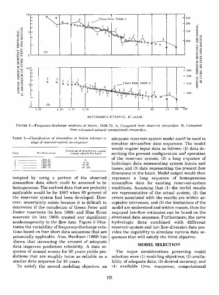
Observed streamflow data at Sale1n are not adequate for estimating the low-flow cl'aracteris­tics required to satisfy the second objActive. Al­though the data sequence is long enoug'l, the data are not homogeneous. A compariscn of the frequency-discharge relations shown in figure 2 supports this conclusion. These relations are based on 192~ 73 data sequences of monthly streamflow at Salem. Classification of these data into four shorter data sequences representing in­creased stages of reservoir-system development is shown in table 2. Figure 2A, based on observed data, exhibits the expected trend of higher annual minimum-monthly discharges with increased low-flow augmentation from the reservoir system. There is some overlap of the four classes of data as should be expected since the reservoir system does not entirely eliminate variations in reservoir-system inflqw. Figure 2B is based on the natural (unregulated) monthly flows that were estimated for reservoir-system model input (see ''Streamflow Data" subsection of subsf'(]Uent sec­tion "Input Data Preparation"). The more com­plete mixture of the four classes of data in the latter figure illustrates the nonhomogeneity in­troduced into the observed data by rrogressive reservoir-system development. N onhcmogeneity is also introduced by other types of basin de­velopment (for example, urbanization, changing agricultural practices, and other changing land uses). However, these additional contributing fac­tors are not as easily illustrated and are not as significant as those attributable to reservoir­system development.

Prediction of the effects of the present Wil­lamette River basin reservoir system could be at-

TABLE 1.-Selected information for the 13 reservoirs in the Willamette River basin reservoir system

Control point

number 1

10 11 2-! 12

13 14

15 16 18 23 25 21 22

1See figure 1.

Reservoir name

Hills Creek _____________ _ Lookout Point ___________ _ Dexter3 ________________ _

Fall Creek ______________ _

Cottage Grove ___________ _ Dorena _________________ _

Cougar _________________ _ Blue River _____________ _ Fern Ridge _____ _ Detroit __________ _ Big Cliff' Green Peter _____________ _ Foster __________________ _

Strear;:. name

Useable capacity lacre-ftl

Middle Fork Willamette River ___________ ____ 240,000 _____________________ do______________________ 349,000 ______________________ do_________________ 4,800 Fall Creek ltnbutarv to

Middle Fork Willamette River!. Coast Fork Willamette River ____________ _ Row River !tributary to Coast

Fork Willamette River!. South Fork McKenzie River _________________ _ Blue River \tributary to McKenzie RIVer! ____ _ Long Tom River ___ · __________________________ _ North Santiam River __________________ _ --- --- ________________ do ___________ _ Middle Santiam River ______________ _ South Santiam River __________________ _

115,000 30,100

70,500 165,000

85,000 110,000 340,000

2,400 333,000

33,200

2FC. flood control; N. navigation; I, irrigation; P, power; RR. reregulation. 3Small reregulatmg reservoir.

H4

Drainage Date Authorized area regulation purpose 1mi2 1 began or use2

389 Aug. 1961 FC,N,l,P 911 Nov. 1953 FC,NJ.P 911 Nov. 1953 RR,P

184 Jan. 1966 FC,NJ 104 Oct. 1942 FC,N,I

265 Oct. 1949 FC,NJ 208 Sep. 1963 FC,NJ,P

88 Oct. 1968 FC,N,I 252 Nov. 1941 FC,N.[ 438 Jan. 1953 FC.N,l,P 438 Jan. 1953 RR,P 277 Oct. 1966 FC,N,l.P -!94 Dec. 1966 RR,FC,P

Class from Table 3 250

4---- 200

~ 3 1 5 150

100

3

(A) 3L--J--------~----~----~-----------J------------~----~----~--~--~

10 --~

"""' 5f-

1.01

3 0

(B)

1 •) 0 0

1. 05 1.11

_Class from Table 3 3

h 1 ~ ). 1 ...L ~~ -' k 3 4 1

- 250

- 200

- 150

- 100 2 ~<>o~IOO oo <A __.r-..._

2 3 -1 1 r ~ v <l .......__

10 25 50 100

RECURRENCE INTERVAL. IN YEARS

FIGURE 2.-Frequency-discharge relations at Salem. 1926-73. A, Computed from observed streamflow. B. Computed from estimated natural (unregulated) streamflow.

TABLE 2.--Classification of streamflow at Salern relevant to stage of reservoir-system development

Class

.3 --------------4

Penod of record

1926--41 1942-52 1953-66 1967-73

Percentage of present total useable storage capacity developed

0 6--11

29-76 95--100

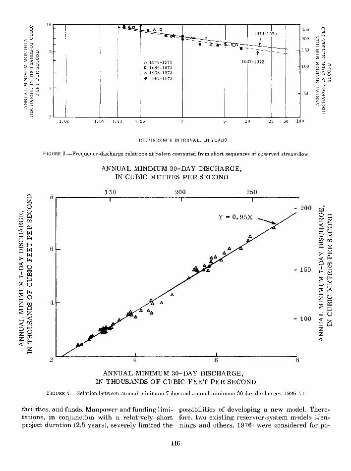
tempted by using a portion of the observed streamflow data which could be assumed to be homogeneous. The earliest data that are probably applicable would be for 1967 when 95 percent of the reservoir system had been developed. How­ever, uncertainty exists because it is difficult to determine if the completion of Green Peter and ,Foster reservoirs (in late 1966) and Blue River reservoir (in late 1968) created any significant nonhomogeneity in the flow data. Figure 3 illus­trates the variability of frequency-discharge rela­tions based on four short data sequences that are potentially applicable. Also, Hardison (1969) has shown that increasing the amount of adequate data improves prediction reliability. A data se­quence of annual events for 50 years yields pre­dictions that are roughly twice as reliable as a similar data sequence for 10 years.

To satisfy the second modeling objective, an

adequate reservoir-system model could be used to simulate streamflow data sequences. The model would require input data as follows: (1) data de­scribing the present configuration anc operation of the reservoir system; (2) a long s'?.quence of hydrologic data representing system inputs and losses; and (3) data representing the p:-:-esent flow diversions in the basin. Model output would then represent a long sequence of homogeneous streamflow data for existing reserYoir-system conditions. Assuming that ( 1) the mo':lel results are representative of the actual system, (2) the errors associated with the results are within ac­ceptable tolerances, and (3) the limitations of the model are understood and within reason, then the required low-flow estimates can be b2sed on the simulated data sequence. Furthermore, the same hydrologic data combined with different reservoir-system and (or) flow-diversio:':l data pro­vides the capability to simulate vario11S data se­quences that will satisfy the third objective.

MODEL SELECTION

The major considerations governing model selection were (1) modeling objectives; (2) availa­bility of adequate data; (3) desired accuracy; and (4) available time, manpower, computational

H5

u 10

s ~50 p:::; w

;:::, ;...., 0.. ;..-,U :300 ...:100 ...:l!J:.. ..,., w ~0 - p:::; E-<E-< E-<ooo G ,----- 1GO 5;:a Zoz Ozo ~~ ::S..:t:u 0 1970-1973 1967-1973

e~o ...... ::nw 100 ~000 0 1969-Hl73 ::::; ~ z

6. 1968-1973 ~>-'0

~~~ -uu • 1967-1973 ~~w

~~~ ;;s 00 ...:< ~

...:< ~ W --< w ww 50 ;:::,~ --<v~J:.. ;::,p:::;

~~ ~~ --<u --<u ga ga 0 0

1. 01 1. 05 1.11 1. :35 5 10 25 50 100

RECURRENCE INTERVAL, IN YEARS

FIGURE 3.-Frequency-discharge relations at Salem computed from short sequences of observed streamflow.

ANNUAL MINIMUM 30-DAY DISCHARGE, IN CUBIC METRES PER SECOND

150 200 250 Q 8 z 0 - 200 ~ .. u

~~ OQ Om o::z 0:::~ <o ~~ ::r::u

u~ uP-t ram 00 ~ Qp::; -~ 6 Q ~ ~~

~ ~ ~Pot

~ u Cloo ·~ I - t-o:;

t- p:)

§~ ~B ;:J~ ~~ ~0 -u

4 z -Zoo -p:)

-Q ~ ;:J ~z HU H< §~ <00 ;:J;:J z zO z z::r:: < <~

z - 2 8

ANNUAL MINIMUM 30-DAY DISCHARGE, IN THOUSANDS OF CUBIC FEET PER SECOND

FIGURE 4.-Relation between annual minimum 7-day and annual minimum 30-day discharges, 1926-71.

facilities, and funds. Manpower and funding limi- possibilities of developing a new model. There­tations, in conjunction with a relatively short fore, two existing reservoir-system m0dels (Jen­project duration (2.5 years), severely limited the nings and others, 1976) were considered for po-

H6

tential application to the Willamette River basin reservoir system. These models are the HEC-3 model developed by the U.S. Army Corps of En­gineers ( 1968) and the SIMYLD II model de­veloped by the Texas Water Development Board ( 1972).

The HEC-3 model exhibited major advantages as follows: ( 1) 8 of the 13 reservoirs in the Wil­lamette River basin reservoir system are used for power generation, and power-release modeling is possible with HEC-3 but is not possible with SIMYLD II; (2) most of the minimum-flow re­quirements in the Willamette River basin are variable by season which can be expressed using HEC-3, but these requirements must be ex­pressed as a yearly average in SIMYLD II; and (3) the more flexible expression of operating rules permitted by HEC-3 made it possible to define better the actual operating rules of the Wil­lamette River basin reservoir system. These limi­tations of SIMYLD II could have been overcome by additional programing had sufficient time been available.

The Portland District of the Corps of Engineers had used the HEC-3 model for preliminary analyses in the Willamette River basin and had

already assembled a considerable amount of di­rectly applicable input data. This advantage, combined with the fact that no revisions of the HEC-3 program were required, resulted in the selection of HEC-3 as the most directly applicable reservoir-system model for this study.

INPUT DATA PREPARATIOP

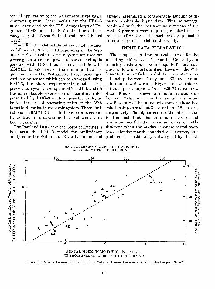
The computation time interval selected for the modeling effort was 1 month. Generally, a monthly basis would be inadequate for estimat­ing low flows of short duration. However, the Wil­lamette River at Salem exhibits a very Etrong re­lationship between 7 -day and 30-day annual minimum low-flow rates. Figure 4 shows this re­lationship as computed from 1926--71 st~eamflow data. Figure 5 shows a similar relationship between 7 -day and monthly annual ninimum low-flow rates. The standard errors of these two relationships are about 3 percent and 18 percent, respectively. The higher error of the latter is due to the fact that the minimum 30-day and minimum monthly flow rates can be sigrificantly different when the 30-day low-flow per~od over­laps calendar-month boundaries. However, this problem is considerably outweighed by the ad-

ANNUAL MINIMUM MONTHLY DISCHARGE, IN CUBIC METRES PER SECOND

8 100 150 200 250

~~ 200 t3o ~ p:;U 00 -<~

A P::z ::r:;rn -<o UP:: Gu ra ~ A Y = 0. 87X 01=4 ra~

~E-1 6 AA om A ~p:; -<~ A A

0~ A <t::~ .~ A 150

o1=4 t-u ,rn

t-~ ~- ~p:; :::>1=0 ~:::> :::>E-1 _u

A ~~ z~ A -~ ~0 4 A ~~ ...:loo. A AA A ~1=0 -< 0 A ...:l:::> :::>z 100 ..:r:U z~ A :::>z Z:::> 1. A z-..:r:g z

-< E-1

~ 2 2 4 6 8 10

ANNUAL MINIMUM MONTHLY DISCHARGE, IN THOUSANDS OF CUBIC FEET PER SECOND

FIGURE 5.-Relation between annual minimum 7-day and annual minimum monthly discharges, 1926-71.

H7

vantages of using monthly data in the model (that is, availability of data and computation reduc­tion). Also, since the total travel time for flows to traverse the length of the basin is only on the order of days, the monthly time frame eliminates the need of any streamflow routing.

STREAMFLOW DATA

The HEC-3 model requires definition of the total streamflow that would occur at each control point under natural conditions (that is, unaf­fected by regulation, flow diversions, and so forth). The U.S. Army Corps of Engineers (writ­ten commun., 1974> provided adequate input data for unregulated, monthly streamflow at all con­trol points for the period 1926-69. They had de­veloped these data using correlation and water­budget computations. It was deen1ed imperative to extend these natural streamflow data through the severe drought year of 1973 (which was also the first year of intensive data collection for DO modeling).

Therefore, at each control point, an attempt was made to develop a relationship for extending the Corps data by correlating the Corps data with observed streamflow at an index station. An index station, in this context, is defined as a streamflow gaging station at which streamflow is

unaffected by regulation and (or) diversions. A

1

satisfactory relationship could not always be ob­. tained using a single index station, ir which cases two index stations were used. Selection of the applicable index station(s) for each control point involved a trial-and-error process to simultane­ously minimize the standard error and maximize the correlation coefficient of the relationship. At a few control points the relationships developed by using gaging station data were judged inadequate because the standard error was too high and (or) the correlation coefficient was too lovr. To develop acceptable relationships at these control points it was necessary to use one (or two) upstream con­trol points as the index station( s ). Table 3 sum­marizes the final relationships used for extending the unregulated streamflow for each control point.

RESERVOIR CHARACTERISTICS

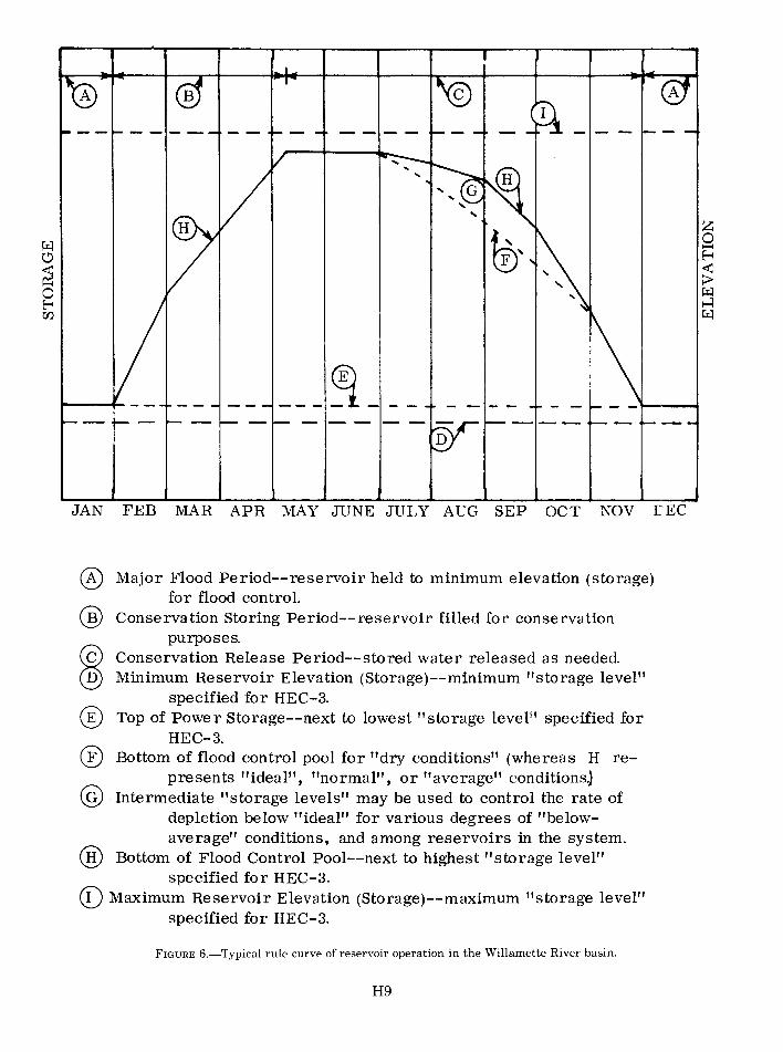
Physical properties of the reservoirs plus power generation data and operating rules were ob­tained from the Portland District of the U.S. Army Corps of Engineers (written commun., 1974). Figure 6 illustrates a typical operating rule curve that is applicable to each reservoir. The storage data used to define the individual rule curves for the HEC-3 model are tabulated in table 4.

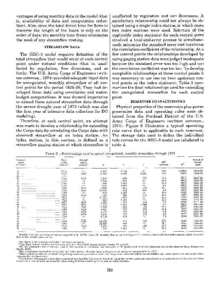
TABLE 3.-Relationships used to extend unregulated, monthly streamflouJ through 1973

Control Fn·st Second Period of pomt mdex mdex SE3 record

number' statwn" statwn2 I percent I R" used

10 -------------- 1448 141 0.561 113~ 141 10.6 0.990~ 1959--69 11 H7.5 1~65 .5.190 0 630 0.360 10.0 .9919 1940--69 2~ 15 1 1:2 ------------------------------- 15~5 152.5 :2.365 .690 .:213 16 6 .9910 19~0--69

~1 1475 141 7.506 .9~.5 1"1 10.6 .9916 1940--69 1:3 1525 141 .980 1.058 1"1 12.6 .9953 19~0--69

u 15~5 ,., 1 ')')'1 1.005 ,., 9-! .9978 19~0--69 ~2 1.525 15~5 2.665 .62~ .478 10.4 9973 19~0--69

~3 1.5:25 1475 16.223 .3~9 .605 9.6 .99~7 19~0--69

1.5 1592 1'1 3.58 1.200 14 1 13.0 .984.5 19.58-69 16 1611 1615 1 797 .868 .146 1~.2 9937 1964--69 ~~ 69~3 141 17 773 .674 14 1 HA 9738 19~0--69

~.5 "9~~ 141 203 1.266 14 1 12.2 9889 1940--69 18 16615 1670 1.291 .929 .176 9.8 .9982 19~1-69 ~6 ----------------------------- 166.5 1670 1.011 1.264 -066 88 .9983 1941-69 ~8 ---------- -- ---------- "9~.5 "9~6 2.419 .838 134 13.8 .9877 19~1-69 21 1850 1870 3.061 .7.5.5 .230 1~ 6 .9922 19~8-69

32 18.50 1870 ~.17.'1 .820 17.5 86 .9973 19~8--69 39 18.50 1870 .5.181 730 .27.5 85 9974 1948-69 :2:3 -- ---- 1790 1'1 6 719 919 (41 76 .9906 1940--69 25 15 1 ~0 ---------- 1825 1790 10 11.5 .210 .703 12.5 .9867 1940--69 ~9 18.50 14 1 :29 36S .840 ,., 1.5.4 .988~ 19~0--69

.50 6 948 "949 l.178 .88.5 .160 12.7 .9906 1941-69

.51 "950 ,., 707 1.0.58 1"1 1.5.0 .98.59 19~1-69

Month!) flow at a control pomt can be computed hy X =a }_·bzc. where X= monthly flow at the control pomt; Y =monthly flow at the first index station; and Z =monthlv flow at the second mdex statwn

1See figure 1 for locatiOns and table 1 for reserYmr names °Four-digtt statwn numbers are the yyyy porhon of the USGS gaging-statwn number 14--yyyyOO. "SE, the standard error of estimate, and R. the correlatwn coefficient, are measures of the goodness of fit of the computed data to the observed data I Draper and

Smith, 19661. "Best correlation obtained by usmg only one index station Monthly flows at these control points are computed by X =a yb. 'These control pomt5 are at small reregulating reservoirs JUSt downstream from large resen·oirs and reqmre no streamflow data since there iS no additwnal mflow

between the two reservoirs. "Correlation with gagmg-statwn data considered unacceptable. Correlation was made usmg one lor two 1 upstream control point Is 1 as mdex statwnls 1. 9xx denotes flows

computed at control pomt xx usmg the relatwnship between control point xx and its mdex statwnl s 1

HS

--- ~---

JAN FEB MAR APR MAY JUNE JULY AUG SEP OCT NOV IEC

@ Major Flood Period--reservoir held to minimum elevation (storage) for flood control.

@

®

Conservation Storing Period--reservoir filled for conservation purposes.

Conservation Release Period--stored water released as needed. Minimum Reservoir Elevation (Storage)--minimum "storage level"

specified for HEC-3. Top of Power Storage--next to lowest "storage level'' specified for

HEC-3. ® Bottom of flood control pool for "dry conditions" (whereas H re­

presents "ideal", "normal", or "average" conditions.) @ Intermediate "storage levels" may be used to control the rate of

depletion below "ideal" for various degrees of "below­average" conditions, and among reservoirs in the system.

@ Bottom of Flood Control Pool--next to highest "storage level" specified for HEC-3.

([) Maximum Reservoir Elevation (Storage)--maximum "storage level" specified for HEC-3.

FIGURE 6.-Typical rule curve of reservoir operation in the Willarnette River basin.

H9

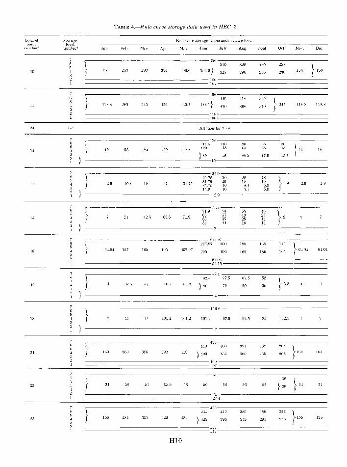
TABLE 4.-Rule curve storage data used in HEC-3

Control Storage Reservmr storage 1 thousands of acre-feet 1

pomt level number' number" Jan Feb. Mar. Apr. May .June .July Aug Sept. Oct. Nov. Dec.

I .356 6 } 340 325 295 238

} 156 .s

156 250 290 330 350.6} 156 10 4 350.6 325 290 260 230 3

156 107

7 456 6 'l 430 410 345 } 5

443.1} 11 4 J 118 8 265 340 420 443.1 410 360 310 245 118.8 118.8 3 2 118.8 1 106.6

24 1-7 All months: 25.4

7 125 6 } 117.5 110 90 6.5 30

l1o 10 58 84 109 117.5 100 95 65 35 15 10 12

} 50 45 22.5 17.5 13 5 J 10

7 32.9 6 ~ 31.75 30 25 18

l39 5 31.75 26 18 10

13 4 J 2.9 10.8 19 27 31 75 31.75 16 8.4 5.9 f . 2.9 2.9 3 11.9 10 7.7 5.9

\. I 2.9

7 77.5 6 -~ 71.9 70 55 40 )~ 5 65 .57 40 25

14 4 J 24 42 5 60.5 71.9 35 35 25 14 s 3 30 24 19 14

7 219 .. 27 6 } 207.97 200 190 165 115

l6404 .5

6404 6404 15 4 127 162 195 207.97 200 190 160 130 105 J . 3

64.04 54 15

7 89.1 6 t 82.8 77.5 67.5 52 I 5

5.8 16 4

' .37.5 .57 76.5 82.8

} 80 70 50 30 J 4

3

4

7 116.9 6 ~ 5

18 4

' -!3 81 101 2 101.2 1012 97.5 92.5 85 32.5

3 .-, }

7 430 6 't 410 400 370 338 265

}160 5

21 -! J 160 280 336 392 HO ) -!00 350 300 255 205 160

3 160

97

7 61 6 l 38

} 31 5

31 } 36 22 4 '

38 46 53 .. 5 56 56 56 56 56 31 3

31 27 4

7 455 6 } 434 -!13 386 350 262

} 1.55 5

1.55 284 355 422 43-! 155 23 4 } 425 395 345 295 245 3

155 115

HlO

TABLE 4.-Rule curue storage data used in HEC--3-Continued

Control pomt

number'

25

Storage len• I

number2

1-7

. Jan Feb .

1See figure 1 for locations and table 1 for reservOir names.

Mar Apr

Resenmr storage 1thousands ol acre-teet>

Ma\' .June ,July Aug. Sept Oct NO\ Dec

All months· 4.53

2 See figure 6 for storage-level definitwns. Storage level numbers m this table coinnde with lettered items m figure 6 as follows: Levels 1 through 3 corrEspond to hnes D. E. and F: levels 4 and 5 are within region G: and levels 6 and 7 correspond to hnes H and I.

DIVERSION DATA

The Corps also provided the diversion data (written commun., 1974) which they had obtained from the Bureau of Reclamation. These data re­flect net depletions attributable to irrigation and municipal and industrial water-supply demands. Table 5 summarizes the estimated net depletions (withdrawals from the system) or return flows (returns of excess withdrawals to the system) for the years 1970, 1980, 2000, and 2020 at each di­version point (fig. 1).

CLIMATOLOGICAL DATA

Evaporation data used in the HEC-3 model are computed from the relationships shown in figure 7. These relationships were obtained from the U.S. Army Corps of Engineers (written commun., 1974). These data, reflecting total evaporation, could be adjusted to reflect net evaporation by adding average basin precipitation to each value. However, this represented a significant data preparation effort and was ignored for the pur­poses of this report.

OTHER DATA

The Corps (written commun., 1974) also pro­vided the following miscellaneous data: ( 1) minimum desired flows at all control points, (2) maximum desired flows at all control points, and ( 3) all of the data pertaining to shortage declara­tion (permissible depletion of desired reservoir storage to provide desired flows) in the reservoir system.

MODEL CALIBRATION

Many types of models (such as DO models and streamflow-routing models) must be calibrated. As discussed by Hines, Rickert, McKenzie, and Bennett (1975), this procedure is required to ad­just certain model parameters so that model re­sults (for a particular set of observed input data) adequately represent the observed Hreal world" results. HEC-3 contains no model parameters of

this nature, thereby eliminating the need for calibration.

MODEL VERIFICATION

An important aspect of any modeling effort is model verification. That is, model results must be compared to observed, "real world" data to judge whether or not the model is a valid predictive tool.

The present reservoir system of 13 reservoirs in the Willamette River basin was not ccmpleted until 1968. To avoid any anomalies that may have existed in the operation of the system with the addition of the last few reservoirs, tr. e period of 1970 through 1973 was selected for the verifi­cation procedure. The 1973 reservoir-sys-l;em con­figuration and operating rules were defined in the model and 1970 (table 4) diversions were assumed representative of water demands for the verifica­tion period. Unregulated monthly streamflow and evaporation data for 1970-73 were used to define the system inputs and losses.

Table 6 (lines 6 and 7) summarizes the stream­flow computed by HEC-3 (Qcl and the observed streamflow (Q 0 ) for the Willamette Piver at Salem for the period 1970-73. Both monthly and average annual data are shown. Also tabulated Oine 8) is the total error of each of the computed values (total Qc error in percent of Q 0 ). Differ­ences between model results and observed aver­age annual streamflow at Salem are considered very acceptable. Comparisons of nonthly streamflow values range more widely, from poor to very good.

These total Q c errors are due to differences be­tween the model and the real world for ( 1) inflows to and losses from the system and (2) definition and operation of the reservoir system. A mass­volume balance of an entire reservoir syst.em may be expressed as

IL-Q=~, (1)

where IL represents an algebraic summation of all inputs to the system and all losses from the

H11

TABLE 5.-Flow diversion data used in the HEC-3 model

Control pomt

number'

Net monthly depletwn !return fl.ow1 2 in cub1c feet per second

41

42

45

46

48

39

40

49

.50

51

Year

1970 1980 2000 2020

1970 1980 2000 2020

1970 1980 2000 2020

Jan

1 1 4 5

3 2

34 .53 8:3

124

1970 ------------------- -- 1161 1980 ------------------------ 1291 2000 ----------------------- 1461 2020 ----------------------- 1801

1970 1980 2000 2020

1970 1980 2000 2020

1970 1980 2000 2020

1970 1980 2000 2020

1970 1980 2000 2020

1970 1980 2000 2020

1970 1980 2000 2020

9 8

14 19

17 9

191 7

17 16

1191 181

6.3 87

109 140

1 4 0 0

1171 1341 1.341 1181

24 1111 1181 29

'See figure 1 for locatwns. 2Values m parentheses md1cate return flows

Feb.

3 4 3

11

33 50 84

124

I 131 1271 1431 1711

11 10 17 24

24 17

9 33

19 17

1111 2

66 92

11.3 142

3 6 .3 4

1141 1.3.3r 1281

191

45 21 53

113

Mar.

4 6

3 3 3

10

33 51 79

117

1141 1261 1401 1671

10 9

16 22

21 16

9 31

18 17 191

•)

62 1)5

104 131

I 151 1291 r251

181

41 28 4B

110

Apr.

3 4 3

10

37 .56 86

128

1151 1281 1461 1751

11 10 17 23

22 17

9 3.3

19 17

1101 ')

65 90

109 138

1161 1311 r271

191

44 27 48

105

system, Q is the system output, and llS is the net summation of the storage change in all reservoirs In the system. The IL term is not directly ob­served (nor directly computed by the model) but can be estimated from observed (or computed) values ofQ and llS. Therefore, rewriting equation 1 and subscripting with o for terms related to ob­served data and c for terms related to computed values (model results) yields

(2a)

and

May

6 8

14 18

15 24 47 56

67 107 215 305

1111 1161 1111

1

33 54

120 117

57 84

125 126

41 49

231 232

157 2.36 .342 405

5 14 17 .35

39 90

150 194

.300 46.3 877 864

June

19 24 38 52

44 74

148 177

160 245 551 764

151 3

52 151

91 58

365 349

146 227 400 -!42

10.5 126 754 768

.374 548 890

1,044

11 .3.3 51

12.3

161 .338 568 722

883 1,370 2,797 2,892

July

20 26 40 54

47 78

158 187

197 306 657 931

1211 1211 18

108

98 174 393 377

148 234 38.3 410

112 139 811 829

422 631 994

1.185

9 .31 4.3

120

175 384 591 756

966 1,538 2,971 2,968

Aug

16 21 34 46

37 64

130 15.3

161 254 529 740

1211 1271

121 62

80 1:39 302 285

99 140 224 211

83 102 551 543

320 475 758 898

:3 16 22 68

107 230 377 469

631 964

2,134 1.955

Sept.

5 6

11 17

9 15 .34 .38

86 1.38 278 393

1221 1371 1451 1581

33 50

122 112

46 43 22 16

47 53

179 190

174 250 .389 478

0 4

1.31 14

22 47 84

129

239 .304 668 610

Oct.

0 I 1 I 0 2

121 It' I

1151 1141

42 6f

104 158

1201 1381 1701

11151

11 8 7 9

16 1151 1701 1931

21 17

15.31 1541

60 78

105 1.35

0 1.31

1111 I 191

1301 1671 1851 1951

1411 11601 12391 12951

Nov.

I 11 141 181

1101

38 59 94

137

1141 1301 1521 1921

13 10 14 13

27 10

1351 1341

24 2.3

1341 1211

66 91

110 141

•)

.3 141 171

121 I 1511 1721 1651

28 1521 1831 1881

Dec.

1 1 4 5

3 2 1 5

35 56 87

131

1161 1311 1501 1871

9 8

14 18

16 1

151 161

14 15

1181 1171

63 86

111 137

0 141

1221 1491 1381 1.351

14 1471 1161 10

Table 6 (lines 1-3) summarizes the values of IL0 , ILc, and the ILc error. The latter term is com­puted as

ILc error= xlOO. (3)

Also tabulated are the ilS0 and llSc values (lines 4 and 5). The small reregulating reservoirs (Big Cliff and Dexter) are not included in llS because ( 1) observed data are not available and (2) there was a constant zero storage change for these res­ervoirs in the HEC-3 model. Over 90 percent of

(2b) the ILc values, which are based on the model re-

H12

5 9

1.

8 2.

7 3. 00. ~ ::t: u 25 25 z 6 0 ~ "< ~ 0 0.. "< > 5 ~

z < 0.. ~ ...:I ::t:

4 E-t z 0 ~ 1'1:;:1 C)

< ~ 1'1:;:1 3 > < 0:

1'1:;:1

2

40

AVERAGE MONTHLY AIR TEMPERATURE AT EUGENE, IN DEGREES CELSIUS

10 15

Evaporation rate, Er, in inches per month per acre of surface area is Er = 0. 7 Ep· Total reservoir evaporation, E, in acre-feet is E = A(Er)/12 where A is reservoir surface area. Evaporation is considered negligible for the months November through March.

45 50 55 60 65

AVERAGE MONTHLY AIR TEMPERATURE AT EUGENE, IN DEGREES FAHRENHEIT

FIGURE 7.-Evaporation relations for the Willamette River basin.

H13

20

200

00.

~ t~ ~ .,.... ,.-.;

~ H

~ 150 ~

z g E-~ ~ ~=~ 0 ~" ~ > ~

z <r: ~<

~ 100 s

t~ z 0 ~ ~ 0 ~ ~: ~'t:l > ~

0: ~t:l

50

70

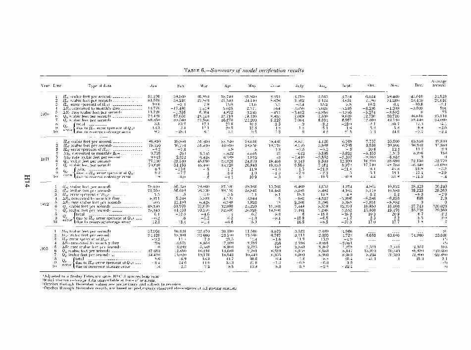
TABLE 6.-Summary of model verification results

Average Year Lme Type of data .Jan Feb Mar. Apr. May June .July Aug. Sept. Oct. Nov. Dec. annual

IL0 !cubic feet per second I _____ 91,190 39,560 25,830 18,740 21,900 8,251 3,719 2,505 3.744 6,524 29,460 43,010 24,520 ILc lcuhic feet per second!_ 81,570 .38,210 27.860 21,540 24,440 8,676 3.592 2,124 3,601 7,1K6 31,260 311,440 24,010

3 ILc error !percent of!L,)i __________ -10.6 -3.4 79 15.0 11.6 5.1 -.34 -15.2 -3.8 10.2 6.1 -10.6 -2.1 4 .:lS" nmverted to monthly flow_ 18,770 -17,490 7,419 5,025 2,771 -564 -3,350 -.5,025 -5,295 -6,206 -1,208 -3,599 -594

1970 5 .:lSc rate !cubic feet per second! 11,720 -1,355 G,.304 Hl72 ::l,245 -451 -3,412 -4,856 -3,356 -5,274 -8,882 0 -75 6 Q

0 !cubic feet per second! _______________ 72,420 .57,050 Hl,410 1.3,710 19,130 S,t\15 7,069 7,5.30 9,039 12,730 30,710 46,610 25,110

7 Qc !cubic feet per second! 69,850 39,56(1 21,560 16,670 21,200 9,127 7,004 6,834 6,9.57 12,460 40,140 38,440 24,090 8 Q rota!.----~--------------------- --3.5 -30 7 17.1 21.6 10.8 3.5 -.9 -9.2 -23.0 -2.1 30.7 -17.5 -4.1 9 efror due tulLe t>rrur !percent ofQ0 1 _ -13 3 -2.4 11.1 20.5 13.3 4.8 -1.8 -.5.1 -1.6 5.2 5.8 -9.8 -2.0

10 due to reservou·-storage error __ 9.7 -21'1.3 6.1 1.1 -2.5 -1.3 9 -4 2 -21 5 -7.3 24.9 -7 7 -21

IL 0 I cubic feet per second! ______ 86,830 39,ROO -~1.8011 38,140 21'1,610 19,430 S,831 4,126 6,768 7,757 3.5,500 63,830 32,640 ILc tcubic feet per second I_ 79,720 :36,770 51,8:30 40,010 28,8.50 19,170 8,170 3,909 6.70.5 8,580 39,900 .'i6,340 31,680

3 ILc error I percent of IL 0 1 _____________ -8 2 -7.6 .1 4.9 8 -13 -7.5 -5.2 -.9 10.6 12.4 -11.7 -2.9 4 .:lS0 converted to monthly flow_ 9,735 263 6,145 4,822 4,545 -21 -612 -5,595 -5,922 -8,453 1,815 -8.296 -138

1971 5 .:lSc rate !cubic feet per second I __ 9,043 2,622 6,428 6,289 1,912 43 -1,410 -3,.5.52 -3,267 -9,160 -8,882 0 0 6 Q0 !cubic feet per second! 77,100 39,G40 4.5.61)0 33,320 24,070 19,450 9,443 9,540 12.690 16,210 33,690 72,130 32,770 I Qc lcuhic teet per second! _ _ ______ 70,680 34,150 45,41111 33,720 26,940 19,130 9,580 7.461 9,97:l 17,740 48,780 56,340 31,6SO 8

Qc { ~~:1to JL~-~;,~;;(p~;~~,;t~f-Q~~-=== -8.::l -13 6 -.5 1.2 11.9 -l.fi 1.5 -21.8 -21.4 9.4 44.8 -::n.9 -3.3 9 -9.2 -7.7 .1 5.6 1.0 -1.3 -7.0 -2.3 -.5 5.1 13.1 -10 4 -2 9

::r:: 10 error due to reservmr-storage error ----- 9 -6.0 -.6 -4.4 10.9 -.3 8.4 -19.5 -20 9 4.4 31.1'1 -11.5 -.4 1--'

*"" 1 IL 0 !cubic feet per second I _______________ 78,040 56,320 79,060 37,100 29.160 15,760 6,469 4,0.52 4.374 4,864 10,070 38,420 30,240 2 ILc !cubic feet per second!_ 73,750 56,610 76,700 39,150 28,840 14.480 5,2t1.5 3.492 4,164 5,119 10,590 35,220 29,360 3 ILc error I percent of IL 0 1 -55 .5 -3 0 55 -1.1 -8.1 -18.3 -13.8 -4.8 5.2 5.2 -S.3 -2.9 4 .:lS11 converted to monthly flow_ 8,911 5.348 5,393 4,107 3,944 5 -980 -4.527 -7,996 -6,086 -6,030 68.5 219

1972 5 .:l8c rate !cubic feet per second! 405 12,180 6,42R 6,289 1,920 -18 -2,206 -3,796 -3,388 -7,951 -8,882 0 0 6 ~~ 11 ~~~:~ f::i ~=~ ~=~~~t =====--~=-===== 69,130 50,970 73,670 32.990 25,220 1.5,760 7,449 8.579 12,370 10,950 16,100 37,740 130,020 7 73,340 44.430 70,270 ~2.860 26,920 14,500 7,491 7,28R 7,552 13,060 19,470 35,220 29,360 8

Qc {~~:\o i£:"-~~;~;(p~~~~,;t-oYQ~,-~-=- 6.1 -12 8 -4.6 -.4 6.7 -8 0 6 -15 0 -38 9 19 3 20 9 -6 7 -2 2 9 -6.2 .6 -3.2 6.2 -1.3 -8.1 -15.9 -6 .. 5 -1.7 2.3 3.2 -8 .. 5 -2.9

10 error due to reservoir-storage error -- 12.3 -13 4 -1.4 -6.6 8.0 .1 16.5 -!-i.5 -37.3 17.0 17.7 18 .7

IL 0 1cub1c feet per second I __________ 37,950 16.420 22,870 20,190 11,500 6,875 3,522 2,489 4,966 (21 ILc 1cub1c feet per second!_ 34,420 18,300 24,660 24.540 13,160 6,767 3,111 2.093 4,722 6,653 63,080 74,960 23,060

3 ILc error I percent of IL 0 1 -9.3 11.-i 7.8 21.5 14.4 -1.6 -11.7 -15.9 -4.9 (21 4 .:lS11 converted to monthly flow ___________ 296 3,572 6,65R 7,109 3,797 336 -2,536 -4,091 -3,081 (2)

1973 5 .:lSc rate !cubic feet per second! 0 ::l,282 5,489 6,003 2.725 -188 -2,889 -3,907 -1,278 -1,571 -7,441 2,157 183 6 Q 0 !cubic teet per second! ___________ 37,6.50 12,8.50 16,210 13,080 7,701 6,539 6,058 6,580 8,047 13,970 70,440 85,930 "23,600 7 Qc !cubic feet per second I 34,420 1.'5,020 19,170 18,540 10,440 6,955 6,000 6,000 6,000 8,224 70,520 72,800 -122,880 R Q rota! ----------------------- -S.6 1li.9 18.3 41.7 35.6 6.4 1.0 -8.8 -2.5 4 -411 .1 -15.3 -3.1 9 ei~;·or due to ILc error I percent of Q 0 1 -9 4 14 6 110 333 21 6 -1 7 -6.8 -6.0 -3.0 (2)

10 tlue to reservOir-storage error _ .8 2.3 7 2 8.5 13.9 8.0 58 -2 8 -22.4 1"1

'Adjusted to a 28-day February since HEG-3 1gnores leap year. 2Final reservOir-storage data unavailable at hme of analysis. 30ctober through December values are prelimmary and subject to revision. "October through December results are based on preliminary observed streamflows at all ga~mg statwns

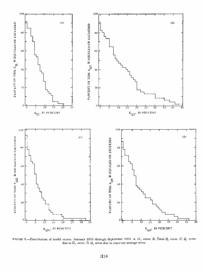
suits, are within ±15 percent of the lL0 values which are based on observed data (table 7 and fig. 8). This is especially gratifying considering the vast opportunity for discrepancies in the ( 1) correlations for natural inflows, (2) diversion data, and (3) evaporation data. The errors in the annual average flow for 1970-73 are all less than 3 percent.

Additional insight to the modeling error can be gained by subtracting equation 2a from 2b and rearranging to obtain

Furthermore, multiplying through by 100/Q0

re­sults in

(Q -Q )

CQO

0

X 100

The three bracketed terms in equation 5, fron1left to right, represent (fig. 8) (1) total Qc error, (2) Qc error due to !Lc error, and (3) Qc error due to reservoir-storage error. Table 6 (lines 8-10) summarizes these errors (with some roundoff er­ror). Generally, errors due to reservoir-storage error are more significant than those due to ILc error (tables 7 and 8 and fig. 8), especially when the total Q c error is large.

Most of the error related to reservoir storage is

due to differences in actual reservoir operation as compared to the reservoir operatior in the reservoir-system model. The summation of both the storage changes and the total storage for 11 reservoirs in the Willamette River barin reser­voir system (Big Cliff and Dexter are orritted) for the rule curves defined for the model are tabu­lated in table 9. Figure 9 illustrates the operation differences between the model and the actual res­ervoir system.

Operational differences are a commor problem in reservoir-release modeling. Rule curves are formulated during the reservoir's design phase in such a way that benefits from the reservoir will be maximized over a long period. Es"entially, they reflect the operation of the reservoir for ((av­erage'' hydrologic conditions. Departures of the hydrologic conditions from ('average'' frequently necessitate deviations from the design rule curve. A good example of such a case is the limited snow­fall in the winter of 1972--73. Even by holding spring flows relatively low, it was only p'1ssible to fill the reservoir system to about 92 percent of desired capacity. Therefore, to meet derired flow objectives in July through September, system storage was depleted to less than 85 :r: 8rcent of desired capacity in August. The HEG-3 model (in its present form) was not capable of such anticipa­tion and only filled the system to about 76 percent and depleted it to less than 65 percent of desired capacity.

Design rule curves (or parts the reo[) may also become outdated if new objectives are considered.

TABLE 7.-Model errors classified by absolute error limits

Percentage of months during the period January 1970 through September 1973 for wh1ch model errors are within absolute error lim1ts of-

Type of model error' 5

percent

EJL _____________ 31.1 EQT _____ 26.7 EQJL _____________ 37.8 EQR _____ 35.6

10 percent

6.±.4 .±8 9 75.6 64.4

15 20 percent percent

91.1 97 8 60.0 71.1 91.1 933 75.6 84.4

25 30 35 percent percent percent

100.0 84A 86.7 911 97.8 97.8 100.0 93.3 9.56 97.8

'These symbols are used lin thts table and in table 8 and figure 81 to mdtcate absolute magmtude of the model errors as follows: EJL -[Lc error 1lme 3, table 61 EQr-total Qc error llme 8, table 61 EQJL -Qc error due to ILc error 1lme 9, table 61 EQR -Qc error due to reservOir-storage error I line 10. table 61

TABLE B.-Summary of modeling errors U.'ith absolute value exceeding 15 percent

Number of

observatwns

Average absolute

error I percent I

{

EQT --­EQJL --­EQR ---

Jan.

.. 0

-----------

Feb

.. Q

23 . .8 8 .. 5

15.3

Mar

4 2 2

17.7 110

6.7

H15

Apr

4 •)

2

31.7 36.9

.±.8

May

4 1 1

35.6 21.6 13.9

Month

June July

4 .. 0 u

Aug.

4 1

21.8 2 .. :3

19 .. 5

Sept.

.. 4

27.3 1.7

2.5.5

.±0 percent

95.6

100.0

Oct.

19.3 2.3

17.0

Nov

32 .. 1 7.4

2HI

45 percent

100.0

Dec.

19.7 10.1

9.6

100

0 w 0 0 w w 0 w 80

w u w X u w X 0:::

w 0 0:::

0 0 w 0 .....:1 GO w

60 ..:r: .....:1 ;:::; ..:r: 0 ;:::; w G' ;a w

...:l ~

w E-< G'

w 40 w 40

~ w E-< ~ ~ E-< 0 ~ E-< 0 z

:20 E-< 20 w z u w 0::: u w 0::: 0.. w

0..

0 0 15 25

ElL' IN PERCENT EQT' IN PER CENT

100

0 0 w 0 w w 0 w w u 80 w 80 X u w :X:

w 0::: 0::: 0 0 0 0 w .....:1 w ..:r: 60

.....:1 60 ;.:.., ..:r: G' ;:::; w G'

w ;a ;a ~ 0::: G' G' w 40 w 40

w w g ~ E-< ~ ~ ~ 0 0 E-< E-< z 20 z 20 w w u u 0::: 0::: w w 0.. Pot

0 25 30 35 15 20 40

EQIL' IN PERCENT EQR' IN PERCENT

FIGURE B.-Distribution of model errors, January 1970 through September 1973. A, ILc error. B, Total Qc error. C, Qc error due to ILc error. D, Qc error due to reservoir-storage error.

H16

TABLE 9.-Summation of total end-of-month storage and monthly storage changes specified by the design rule curces for 11 reservoirs in the Willamette Riuer basin reseruoir system

Svstem January February March April May June st~rage'

End-of-month total ___ ------------------ 715.74 1.417.30 1,812.50 2,186.70 2,306.82 2,306.82 Change dunng month -- ------------------ 0 701.56 395.20 :374.20 120.12 0

System July August September October November December storage 1

End-of-month total 2.224.00 2.067 .. 00 1.809.00 1,24-!.20 715.74 715.74 Change during month -82.82 -157.00 -258.00 -564 .. 80 -.528.46 0

'Storage quantities, shown m thousands of acre-feet, represent summatwn of indi\·idual destgn rule curves for the enttre system, wtth the exceptton of Big Cliff and Dexter reregulatton reservoirs.

--Design Rule Curves

o Observed Data

I!!. HEC-3 :.Iodel Results

2000

rn w c:: E-w ~

~ u w

~ (:::)

~ ~ w 0 <C

~ E-rn

E= z 0 ~ I

i:;.. 0

I c z ~

...:l <C E-0 E-

FIGURE 9.-Comparison of design, observed, and computed reservoir-system storage.

This has occurred in the Willamette River basin where increased flows in late August and in Sep­tember are now used to stimulate fall fish runs. Table 6 readily reveals this effect with Q 0 consist­ently higher than Qc in August and September. Revision of the rule curve definitions in the model would have eliminated this particular bias, but detailed information was not available to make the revision for this study.

Other general possibilities for deviation from the design rule curve at individual reservoirs are (1) floods which require temporary use of the flood control pool, (2) special operational procedures to optimize short-term power production in the

basin (especially if a portion of the total genera­tion capacity is inoperable), and (3) terr.porary storage depletion and (or) discontinuation of re­leases for maintenance reasons.

Another important factor to consider in the dis­cussion of the HEC-3 model errors is the combi­nation of temporary flood storage and the monthly time incren1ent. Several instances can be found where the end-of-month deviatior above the rule curve (fig. 9) is due to a flood occurring late in the month. An examination of ol:'served daily data reveals that the system storage was depleted to the design rule curve shortly into the next month. Evacuation of the flood wat£-v-s any

H17

sooner would have created unnecessary flooding below the reservoirs.

In summary, the verification results were con­sidered acceptable. The HEC-3 model duplicated the actual system fairly well when considering that ( 1) some of the errors are due to the monthly time increment <which tend to balance out over two or more months) and ( 2) the rule curve de­fined in the model could be altered to more closely reflect current operating procedures. The ILc error analysis provided confidence in the input data used to define the natural streamflows, the diversions, and the evaporation for the system as a whole.

APPLICATIONS OF THE MODEL

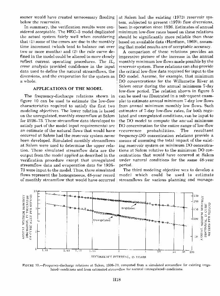
The frequency-discharge relations shown in figure 10 can be used to estimate the low-flow characteristics required to satisfy the first two modeling objectives. The lower relation is based on the unregulated, monthly streamflow at Salem for 1926-73. These streamflow data (developed to satisfy part of the model input requirements) are an estimate of the natural flows that would have occurred at Salem had the reservoir system never been developed. Simulated monthly streamflows at Salem were used to determine the upper rela­tion. These simulated streamflow data are the output from the model applied as described in the verification procedure except that unregulated streamflow data and evaporation data for 1926-73 were input to the model. Thus, these simulated flows represent the homogeneous, 48-year record of monthly streamflow that would have occurred

1. 01 1. 05 1.11 1. ~5

at Salem had the existing (1973) reservoir sys­tem, subjected to present (1970) flow diversions, been in operation since 1926. Estimates of annual minimum low-flow rates based on these relations should be significantly more reliable than those based on available data <Hardison, 1969), assum­ing that model results are of acceptable accuracy.

A comparison of these relations provides an impressive picture of the increase in the annual monthly minimum low flows made possible by the reservoir system. These relations can also provide the critical low-flow data required for input to the DO model. Assume, for example, that n1inimum DO concentrations for the Willarnette River at Salem occur during the annual minimum 7-day low-flow period. The relation shmvn in figure 5 can be used (as illustrated in a suh-;<equent exam­ple) to estimate annual minimum 7 -day low flows from annual minimum monthly low flows. Such estimates of 7 -day low-flow rates, for both regu­lated and unregulated conditions, can be input to the DO model to compute the anrual minimum DO concentration for the entire range of low-flow recurrence probabilities. The resultant frequency-DO concentration relations provide a means of assessing the total impact of the exist­ing reservoir system on minimum DO concentra­tions at Salem relative to the minimum DO con­centrations that would have occurred at Salem under natural conditions for the same 48-year period.

The third modeling objective wc-s to develop a model which could be used to estimate streamflows for various planning and manage-

/ Regulated

5 10 30 100

HECURRENCE INTERVAL, IN YEARS

FIGURE 10.-Frequency-discharge relations at Salem, 1926--73, computed from a simulated streamflow for existing !regu­lated) conditions and from estimated streamflow for naturallunregulated) conditions.

H18

ment alternatives. Such alternatives or condi­tions might include ( 1) different demands on the system (such as 1980, 2000, or 2020 flow diver­sions), (2) different system-operation schemes (such as deemphasis and (or) placing more em­phasis on one or more of the various authorized uses), (3l addition of reservoirs to the system, (4) the occurrence of more severe hydrologic condi­tions (such as more extren1e droughts than have been experienced), and (5) combinations of the above, ad infinitum.

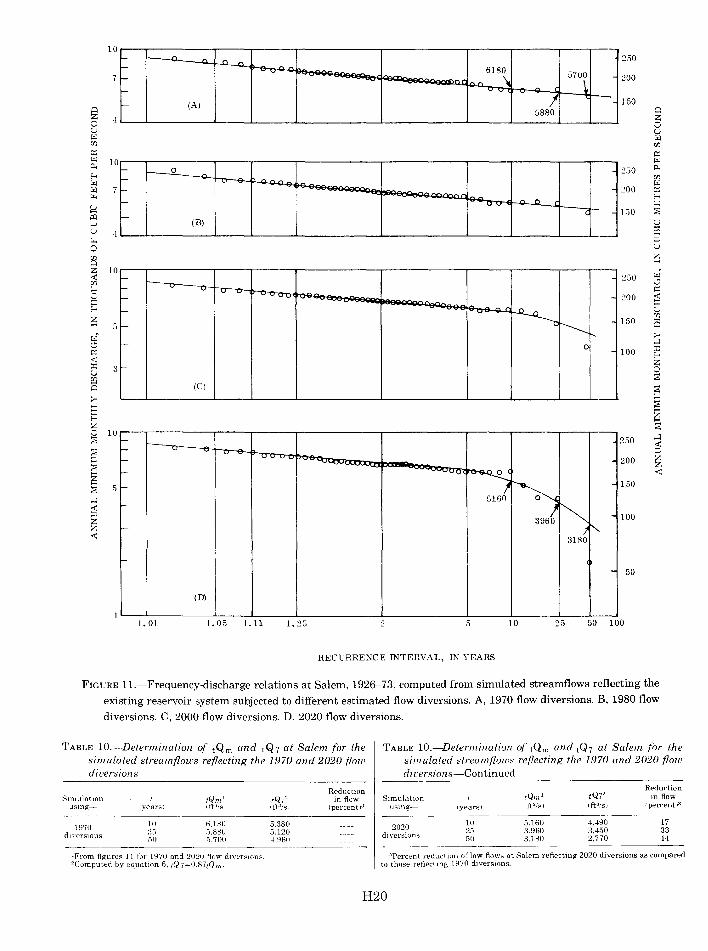
The scope of this report does not permit analysis of all reasonable alternatives. However, to illustrate this type of model application, three additional simulations were performed. Each of these three simulations were identical to the pre­vious 48-year simulation, except that the flow di­versions used were those estimated for the years 1980, 2000, and 2020. Thus, including the previ­ous simulation, 1926--73 data sequences of monthly streamflows reflecting four levels of es­timated flow diversions (table 4) are available for comparison. Frequency-discharge relations of annual minimum monthly flows for all four simu­lations are presented in figure 11. These relations may be used to determine the annual minimum monthly low flow for any recurrence interval (hereafter denoted by tQ m , where t is the recur­rence interval and Qm denotes average monthly flow rate).

Also, as mentioned above, estimates of annual minimum 7-day low flows for any recurrence interval (tQ 7, where t indicates recurrence inter­val and Q7 denotes average 7 -day flow rate) may be obtained using the t Q m data. The relation of annual minimum 7 -day to annual minimum monthly low flows (fig. 5) may be expressed as

(6)

Table 10 summarizes estimates of annual mini­mum monthly and annual minimum 7 -day flows for the 1970 and 2020 levels of flow diversions. Also shown is the percent reduction in these flows resulting from the increased flow diversions proj­ected for 2020 relative to the estimated flow di­versions of 1970. A DO model could be used to assess the impact that the increased flow diver­sions (reduced minimum flows) would have on DO concentrations.

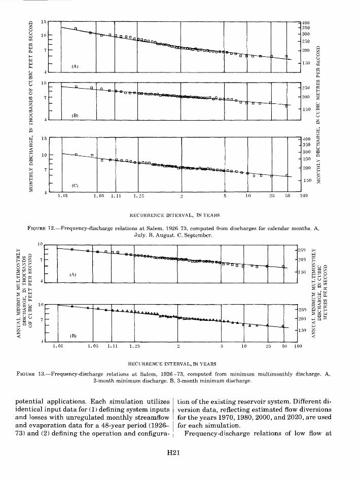
Other low-flow periods may also be useful for assessing potential river-quality problems. For

example, the temperature, sunlight, and flow conditions that combine for critical algal growth conditions may not coincide with the annual minimum 7 -day or annual minimum n1onthly low-flow period. Frequency-discharge relation by calendar months might be more applicable. Fig­ure 12 illustrates such relations for the individual months of July, August, and September b!lsed on the simulated streamflows reflecting the 1970 di­versions. Another potentially useful tool for river-quality assessn1ent might be the annual minun1um flow for multimonth periods. Figure 13 shows frequency-discharge relations for the an­nual minimum flow for consecutive 2- and 3-month periods based on the simulated stream­flows reflecting the 1970 diversions.

Only the Willamette River streamflow at Salem is utilized in the above examplee., How­ever, model results may be obtained at any con­trol point (fig. 1 ). Therefore, similar evaluations could be made for the streamflow at several points for basinwide river-quality assessment.

SUMMARY AND DISCUSSION

A reservoir-system model provides a useful tool for improving an available streamflow data base which consists of streamflow data that have been observed during a period of changing conditions. Applicability of the U.S. Army Corps of En­gineers' HEC-3 reservoir-system model to the W illamette River basin reservoir system is ver­ified by comparing model results with ol~~erved stream-flow at Salem for a 4-year period (1970--73. In general, modeling errors for this verifica­tion period are within reasonable limits. Predic­tive errors could possibly be reduced by (1) revis­ing model input data to better define actual reservoir-system operation; (2) refining unregu­lated streamflow estimates by using water­budget computations along with corr~lation

analyses; and ( 3) using more refined evaporation estimates and including precipitation data in the analysis. This last source of possible error applies to the entire basin. The first two, however, could possibly be isolated to one or more segm~nts of the basin by comparing model results with ob­served streamflow at other control points in the basin. Also, a longer verification period could add increased confidence in model applicabilit:r.

Despite the above limitations, the HEC-3 reservoir-system model is used for four ::-imula­tions of monthly streamflow data to demonstrate

H19

1- r-----..... -1- ~

~ 0" ~

1-~ v -

1- ··~

~ I- ~---~ t-- 0 -f-

(C)

1- r-- -1- v

v 1-

VVv ~

1- ·"'vo ~

1-

516/ ~ -

1-

396t ~ -1-

318~ f'-

1-

- 50

(D)

1. 01 1. 05 1.11 1. 25 2 5 10 25 50 100

RECURRENCE INTERVAL, IN YEARS

FIGURE H.-Frequency-discharge relations at Salem, 1926---73, computed from simulated streamflows reflecting the

existing reservoir system subjected to different estimated flow diversions. A, 1970 flow diversions. B, 1980 flow

diversions. C, 2000 flow diversions. D, 2020 flow diversions.

TABLE 10.-Determination of tQm and tQ7 at Salem for the simulated streamflou•s reflecting the 1970 and 2020 flow diversions

Simulatton tQm 1

using- lyearsl 1tP/s1

1970 10 6,1.'\0

diYersions 25 5,880 50 5,700

1From figures 11 tor 1970 and 2020 flow dlVersions. 2 Computed by equatiOn 6, tQ7=0.87tQ 111 •

Reductwn tQ7" in flow 1lt"/sl I percent 13

5.380 .5,120 4.960

TABLE 10.-Determination of tQm and tQ7 at Salem for the simulated streamflows reflecting the 1970 and 2020 flou.• dit~ersions-Continued

Reduction S1mulatwn 1Qm 1 tQ7" m flow

using- I years I ltt"/sl lft"/si I percent is

2020 10 5,160 4,490 17

diYersions 25 3,960 3,450 33 50 3,180 2,770 44

"Percent reduction oflow flows at Salem reflecting 2020 diverswns as compared to those reflectmg 1970 di verswns.

H20

15.---r---------.-----~-----r------------~----------~------~------r---~--~400

10

(A)

350 300

250

200

150

0 z 0 u

"" rt:J

4----~--------~----~----~------------~----------~------~------~--~--~ 0::

"" 0..

---

f- ~ f- --a---e-~ .... -r-

.~

r- .... ,..,.., f- 0 u r--

-f-(C)

1.01 1. 05 1.11 1. 25 2 5 10 25 50 100

RECURRENCE INTERVAL, IN YEARS

FIGURE 12.-Frequency-discharge relations at Salem, 1926--73, computed from discharges for calendar months. A, July. B, August. C, September.

1. 01 1. 05 1.11 1. 25 2 5 10 25 50 100

RECURRENCE INTERVAL, IN YEARS

FIGURE 13.-Frequency-discharge relations at Salem, 1926-73, computed from mm1mum multimonthly discharge. A, 2-month minimum discharge. B, 3-month minimum discharge.

potential applications. Each simulation utilizes identical input data for (1) defining system inputs and losses with unregulated monthly streamflow and evaporation data for a 48-year period (192~ 73) and (2) defining the operation and configura-

tion of the existing reservoir system. Different di­version data, reflecting estimated flow diversions for the years 1970, 1980, 2000, and 2020, are used for each simulation.

Frequency-discharge relations of low flow at

H21

Salem based on these simulated streamflows for regulated conditions and on the estimated streamflow for natural conditions are used to demonstrate potential applications of simulated streamflow data. Detailed examples illustrate (1) use of low-flow characteristics reflecting existing conditions and those reflecting natural conditions as a basis for assessing the total impact that the existing reservoir system has had on DO concen­trations at Salem and (2) use of low-flow charac­teristics reflecting existing conditions and those reflecting estimated 2020 flow diversions as a basis for assessing the impact that the higher flow diversions projected for the future will have on DO concentrations at Salem. Other potential ap­plications of the reservoir-system model are briefly discussed.

Each reader, of course, is free to pass independ­ent judgment as to the applicability of the simu­lated streamflow data. The author feels that the discharge-frequency relation based on the streamflow data simulated using estimated 1970 flow diversions (fig. 11A) is a more reliable esti­mate of long-term basin response to existing con­ditions that can be obtained by using the limited observed data that are applicable (fig. 3). Also, comparison of figures 11A-D provides a sound es­timate as to the relative decrease in low flows as a result of increased future flow diversions.

Assuming that either (1) the model is adequate as described herein or (2) it can easily be altered to yield more acceptable results, the potential benefits of using it are obvious. It is hard to en vi-

sion any other tool that could provide such flexi­bility for analyzing planning or managemental­ternatives in the Willamette River basin.

REFERENCES CITED

Draper, N. R., and Smith, H., 1966, Ap":llied regression analysis: New York, John Wiley and So:'l.s, Inc., 407 p.

Gleeson, G. W., 1972, The return of a river, the Willamette River, Oregon: Advisory Comm. Environmental Sci. and Technology and Water Resources Inst., Oregon State Univ., Corvallis, 103 p.

Hardison, C. H., 1969, Accuracy of streamflovr characteristics, in Geological Survey research 1969: U.S. Geol. Survey Prof. Paper 650-D, p. D210-D214.

Hines, W. G., Rickert, D. A., McKenzie, S. W., and Bennett, J. P., 1975, Formulation and use of practical models for river-quality assessment: U.S. Geol. Survey Circ. 715-B, p. 13.

Jennings, M. E., Shearman, J. 0., and Bauer, D. P., 1976, Selection of streamflow and reservoir-rdease models for river-quality assessment: U.S. Geol. Survey Circ. 715-E, 12 p.

Rickert, D. A., and Hines, W. G., 1975, A pra-:tical framework for river-quality assessment: U.S. Geol. Survey Circ. 715-A, 17 p.

Texas Water Development Board, 1972, Economic optimiza­tion and simulation techniques for management of re­gional water resource systems, river h'lsin simulation model, SIMYLD-II program descriptio'l: Texas Water Devel. Board, 106 p.

U.S. Army Corps of Engineers, 1968, HEC-3, reservoir sys­tems analysis: Hydrol. Eng. Center U ~ers Manual No. 23-53, 86 p.

U.S. Geological Survey, 1973, Water res0urces data for Oregon-part 1, surface water records: 409 p.

Willamette Basin Task Force, 1969, Appendix M, Willamette basin comprehensive study: Pacific Northwest River Ba­sins Comm. Rept., p. II-1-II-34.

H22