research article evolutionary spectral analyses of a...

Research ArticleEvolutionary Spectral Analyses of a Powerful Typhoon atthe Sutong Bridge Site Based on the HHT

Lin Ma1 Da-jun Zhou1 Ai-min Yuan1 and Hao Wang2

1College of Civil and Transportation Engineering Hohai University Nanjing 210098 China2College of Civil Engineering Southeast University Nanjing 210096 China

Correspondence should be addressed to Lin Ma malinmalin8005126com

Received 29 August 2015 Revised 11 December 2015 Accepted 28 December 2015

Academic Editor Eckhard Hitzer

Copyright copy 2016 Lin Ma et al This is an open access article distributed under the Creative Commons Attribution License whichpermits unrestricted use distribution and reproduction in any medium provided the original work is properly cited

To investigate the nonstationary characteristics of strong typhoons this paper considers the evolutionary spectral characteristics ofstrong typhoons based on the Hilbert-Huang transform (HHT) Discrete expressions are determined for the evolutionary spectralanalysis based on the HHTThe study indicates that the classic empirical mode decomposition (EMD)method fails to extract all ofthe high-frequency fluctuations from wind velocity data and the time-averaged power spectrum obtained directly using the HHTcannot provide the truewind velocity spectrumThedegrees of nonstationarity of different-order IMF components are analysed anda synthesized method of analysing the evolutionary spectrum and time-averaged power spectrum of a strong typhoon is proposedTo avoid the energy leakage problem that exists in HHT spectral analyses the Gram-Schmidt method is used to orthogonalize theintrinsic mode function (IMF) components The study indicates that when the orthogonalization is implemented in accordancewith the sequence from high-order IMF components to low-order ones the orthogonalized components retain the same goodHilbert property as that of the IMFs The synthesized method proposed yields a time-averaged power spectrum that is consistentwith the Fourier spectrum in value and can produce the energy distributions of a typhoon in the time and frequency domainssimultaneously

1 Introduction

As the span of a bridge increases the wind load plays anincreasingly important role in its design Determining anaccurate wind load as a design parameter is critical forensuring the safety of an engineering structure The majorwind characteristics at the site of a bridge or buildinginclude the average wind speed wind direction wind profileturbulence intensity gust factor turbulence integral scaleand power spectral density The power spectral density isan important parameter of fluctuating wind and is usedto describe the energy distribution of the turbulence overdifferent frequencies Currently the fluctuating wind spectrathat are most widely used in wind resistance design forbridges or buildings include the Davenport [1] Harris [2]Kaimal et al [3] and Teunissen [4] spectra among others

The literature onwind turbulence characteristics is exten-sive Lots of authors have published the results of full-scale measurements and wind tunnel tests whereas others

have proposed new mathematical methods of describingturbulence characteristics or algorithms for the numericalsimulation of wind fields On the topic of theoretical modelsSolari [5] published a critical review of the models availablefor representing the longitudinal component of atmosphericturbulence Starting from a critical review of the state ofthe art Solari and Piccardo [6] proposed a unified modelof atmospheric turbulence that is especially well suited todetermining the 3D gust-excited response of a structureUnlike in classic models all parameters addressed in [6]are assigned based on first- and second-order statisticalmoments derived from a broad set of selected experimentalmeasurements Solari and Tubino [7] investigated the two-point coherence function of the different components ofturbulence and suggested a physical principle to establish anappropriatemodel of the two-point coherence function of thelongitudinal and vertical components thereby completingthe statistical model of turbulence The proper orthogonaldecomposition (POD) approach offers efficient tools for

Hindawi Publishing CorporationMathematical Problems in EngineeringVolume 2016 Article ID 4143715 18 pageshttpdxdoiorg10115520164143715

2 Mathematical Problems in Engineering

formulating a model of a turbulence field based on principalcomponents Tubino and Solari [8] proposed a representationof turbulence based on a double application of the POD

In recent years researchers have performed many fieldmeasurements of the wind characteristics at bridge sites[9ndash15] Using the wind data obtained from the StructuralHealth Monitoring System (SHMS) Xu et al [9] studied themean and turbulent wind characteristics of Typhoon Victorat the site of the Tsing Ma Bridge in Hong Kong It wasfound that certain features of the wind structure and bridgeresponse were difficult to consider in the analytical processthat is currently used to predict the buffeting response oflong suspension bridges as the bridge is surrounded by acomplex topography and the wind direction of TyphoonVictor varied during its passage Miyata et al [10] analysedfull-scale measurement data observed on the Akashi-KaikyoBridge during strong typhoons The power spectral densityand spatial correlation of the longitudinal velocity fluctu-ations were analysed These authors found that the spatialcorrelation of two points was well represented not by anexponential formula but rather by an alternative coherencefunction based on isotropic turbulence theory To derivea model of turbulence suitable for buffeting calculationsregarding the Stonecutters Bridge in Hong Kong Hui et al[11 12] studied the mean wind turbulence intensities windpower spectra integral length scales and wind coherences ofthe bridge

Using statistical theory Wang et al [13] analysed thestrong wind characteristics of Typhoon Matsa the buffetingresponse characteristics of the cable and deck of the RunyangYangtze Bridge and the variation in the buffeting responseRMS versus the wind speedThe results obtained in this studyserved to validate the credibility of current techniques inbuffeting response analysis theory Based on field measure-ments of Typhoon Nuri at the Macao Friendship Bridge siteSong et al [14] proposed that the value of the integral scaleincreased when the eye wall of Typhoon Nuri passed overthe field measurement site In the eye wall of the typhoonthe horizontal spatial correlation was relatively strong andthe horizontal spatial correlation spectrum decayed slowlywith increasing frequency Liu et al [15] compared the windcharacteristics of typhoons and strong monsoons at the siteof the Xi-Hou-Men Bridge The similarities and differencesof wind characteristics between typhoons and monsoonswere analysed Wang et al [16] analysed the recorded real-time wind data measured at the Sutong Yangtze Bridge sitein detail to generate the wind-rose diagram mean windspeed and direction turbulence intensity turbulence integralscale and power spectral density and conducted comparativeanalyses among the inhomogeneous wind characteristics ofthree strong wind events including the Northern windTyphoon Kalmaegi and Typhoon Fung-Wong Wang et al[17] analysed the buffeting responses of the cable-stayedSutong Bridge with the wind spectra used in the design phaseand those obtained experimentally from a long-term SHMsystem to compare the actual buffeting response with designpredictions

In previous studies the Fourier transform has often beenused to obtain wind spectrum information based on the

assumption of stationarity However several studies haveshown that powerful typhoons exhibit strongly nonstationarycharacteristics and that lots of abrupt instantaneous pulsesoccur in strong typhoons Therefore to accurately describethe nonstationary characteristics of powerful typhoons it isnecessary to study their evolutionary power spectra [18]

Because of the limitations of theory it is difficult touse the Fourier transform to analyse a nonstationary signalFirst Fourier theory defines harmonic components over alltime and each frequency exists in a complete harmonicform in the time domain thus many additional harmoniccomponents are required to simulate uneven nonstationarydata which may induce false harmonic components andenergy divergence Second the Fourier transform lacks thecapability of simultaneous positioning in both the time andfrequency domains The spectral analysis results obtainedusing the Fourier transform represent the time-averagedspectral distribution Finally the time resolution and fre-quency resolution of a signal are related to each other and theFourier transform fails to automatically adjust the resolutionsin the time and frequency domains depending on the signalcharacteristics

To address the inadequacy of Fourier analysis researchershave proposed time-frequency analysis methods in whicha time-frequency transform is applied to expand the signalenergy in the time-frequency plane to reflect the process ofvariation of a signal in the time and frequency domainsSuch a time-frequency analysis can describe the changingregularity of a signalrsquos spectrum over time Commonly usedtime-frequency analysis methods include the short-timeFourier transform (STFT) the Winger-Ville distribution thewavelet transform and the Hilbert-Huang transform (HHT)

Huang et al [19] proposed a revolutionary method ofsignal decomposition called empirical mode decomposition(EMD) The EMD components possess the Hilbert propertythat is a time-frequency distribution of these componentsthat bears an actual physical meaning can be obtained byapplying the Hilbert transformTheUSNational Aeronauticsand Space Administration refers to this new time-frequencyanalysis method as the HHT The essence of the method isto decompose an original signal into its different fluctuationsand trends at different scales thereby obtaining a series ofdata with different size characteristics

Although researchers havemade considerable progress inthe field of time-frequency analysis the amplitude spectrumobtained via the direct wavelet transform or the HHT has acompletely different mathematical definition from and offersno quantitative comparability with the traditional Fourierspectrum It is difficult to explain the physical meaning of theamplitude spectrum obtained via a wavelet transform or theHHT Priestley [20] proposed the concept of an evolutionaryspectrum by generalizing the power spectrum of a stationaryrandom process The evolutionary spectrum as a conceptualextension of the power spectrum of a stationary randomprocess can accurately describe the changing characteristicsof a spectrum over time The evolutionary spectrum at anyinstant of time has the same physical significance as thepower spectrum of a stationary random process Thereforethe evolutionary spectrum is considered to possess a good

Mathematical Problems in Engineering 3

physical interpretation However parameter estimation foran evolutionary spectrumhas always been a difficult problemin which both the power spectral density function and thetime and frequencymodulation functionsmust be estimated

Spanos and Failla [21] studied parameter estimationfor an evolutionary spectrum based on the wavelet trans-form They calculated the evolutionary spectrum using thefrequency-domain expression of a wavelet function Ding etal [22] discussed the estimation of the evolutionary spectrumof a nonstationary process using the time-domain waveletexpression and wavelet transform coefficient and studied theevolutionary spectra of the wind velocity and bridge responsewhen Typhoon Matsa crossed the Runyang Yangtze Bridgesite

Wen and Gu [18] considered the HHT spectral analysisof a nonstationary process and presented the conversionrelationship between the Hilbert marginal spectrum andthe Fourier energy spectrum However that work did notconsider the energy leakage problem caused by incompleteorthogonality of the EMD components Hu and Chen [23]proposed a method of estimating the local spectral densitybased on orthogonal EMD components applied the methodto the acceleration records of the El Centro and Taft wavesand studied the evolutionary spectral characteristics of theseseismic waves

In the literature [18 23] it is assumed that the energyof each component is always equal to half the energy of thecorresponding analytical signal As noted by Wen and Gu[18] for a high-frequency component this assumption leadsto only a small error because a sufficient number of wavesare present However this assumption is not always validfor a low-frequency component When the amplitude of alow-frequency component is large a large error could beincurred Furthermore the above-mentioned work failed todiscuss the problemofmodemixing in EMDwhich leads to afailure of HHT analyses to provide complete power spectruminformation The Hilbert energy spectrum presented in[18] is consistent with the Fourier power spectrum at lowfrequencies but it is considerably lower than the Fourierpower spectrum at high frequencies However regardless ofthe analysis method used the total energy spectrum or time-averaged power spectrum should be consistent or should atleast satisfy the conservation of energy Therefore it appearsthat there is still some deficiency in the current method ofHHT evolutionary spectrum analysis

This paper considers the evolutionary spectrum charac-teristics of a powerful typhoon based on the HHT Discreteexpressions for the evolutionary spectrum based on the HHTare deduced and the Gram-Schmidt method is used toorthogonalize the EMD components to avoid energy leakageduring the analysis of the typhoonrsquos evolutionary spectrumThe paper discusses the details of the problem of the missinghigh-frequency fluctuations in the time-averaged spectrumobtained using the HHT Based on analyses of the degrees ofnonstationarity of the EMD components this paper proposesa synthesizedmethod for studying the evolutionary spectrumand time-averaged spectrum of a typhoon This synthesizedmethod can avoid the deficiency of the HHT when analysingthe evolutionary spectrum of a strong typhoon and can be

used to study the nonstationarity characteristics of powerfultyphoons

2 Brief Review ofthe Hilbert-Huang Transform

21 Instantaneous Frequency The widely accepted definitionof the instantaneous frequency is that it is the derivative ofthe phase of the signal [24ndash26] To obtain the instantaneousfrequency a real signal 119909(119905) should be converted into ananalytic signal 119911(119905) in the form of a complex function Thecorresponding imaginary part can be obtained from theHilbert transform of the original signal

119910 (119905) =

1

120587

119875int

infin

minusinfin

119909 (120591)

119905 minus 120591

119889120591 (1)

where 119875 denotes the Cauchy principal valueFrom this definition the following analytic signal is

obtained

119911 (119905) = 119909 (119905) + 119894119910 (119905) (2)

Although there are many ways to define the imaginarypart of the signal the Hilbert transform provides a meansof defining the imaginary part such that the result is uniqueEquation (2) can be expressed in polar form as

119911 (119905) = 119886 (119905) 119890119894120579(119905)

(3)

where

119886 (119905) = [1199092

(119905) + 1199102

(119905)]

12

120579 (119905) = arctan [119910 (119905)

119909 (119905)

]

(4)

In this case the instantaneous frequency can be definedas

120596 (119905) =

119889120579 (119905)

119889119905

(5)

The polar form of the analytic signal reflects the physicalmeaning of the Hilbert transform It represents the time-varying amplitude and frequency of a signal However theHilbert transform is only applicable to a monocomponentsignal namely either a signal with a single frequency compo-nent or a narrow-band signal For a multicomponent signalthe instantaneous frequency defined by theHilbert transformis not necessarily a single-valued function of time [26]Because of the lack of a precise definition of ldquomonocom-ponentrdquo the ldquonarrow-bandrdquo requirement has been adoptedas the limitation placed on the data to ensure that theinstantaneous frequency is meaningful However as noted byHuang et al [19] this bandwidth limitation as defined in theglobal sense is overly restrictive yet it simultaneously lacksprecision


22 Empirical Mode Decomposition Huang et al [19] pro-posed the concept of the intrinsic mode function (IMF) toensure the effectiveness of the Hilbert transform An IMF is afunction that satisfies two conditions (1) in the entire datasetthe number of extrema and the number of zero crossingsmust either be equal or differ by at most one and (2) at anypoint the mean value of the envelope defined by the localmaximum and that defined by the local minimum is zeroThe first condition is similar to the traditional narrow-bandrequirements for a stationary Gaussian process The secondcondition ensures that the instantaneous frequency will notexhibit unwanted fluctuations induced by asymmetric waveforms Huang et al [19] noted that even under the worst con-ditions the instantaneous frequency defined by the Hilberttransform of an IMF is still consistent with the physics of thesystem under study The IMF concept offers a more effectivemethod of judging whether a signal is monocomponentIn addition an IMF is not restricted to being a narrow-band stationary signal An IMF can be modulated in bothamplitude and frequency and can be a nonstationary signal

Generally most real signals are not IMFs A real signalmust be decomposed into IMF components Huang et al[19] innovatively proposed the EMDmethod to address bothnonstationary and nonlinear data A specific algorithm forEMD can be found in the relevant literatureThe result of thedecomposition takes the following well-known form

119909 (119905) =

119899

sum

119895=1

119862119895(119905) + 119903

119899(119905) (6)

where 119862119895(119905) (119895 = 1 2 119899) denotes the 119895th component

of the original signal and 119903119899(119905) is the residual signal An

IMF represents an intrinsic fluctuation of a signal and eachmode function at a different time scale corresponds to a wavepattern in the original signal Because IMFs are extractedfrom a signal itself they have self-adaptive features

A signal should be sifted many times before a qualifiedIMF component can be acquired Unfortunately infinitelyrepeated sifting could obliterate the physically meaningfulamplitude modulations making the resulting IMF a purefrequency-modulated signal of constant amplitude To guar-antee that the IMF components retain both amplitude andfrequencymodulations it is necessary to determine a suitabletermination criterion for the sifting process To accomplishthis task Huang et al [19] proposed a method of limitingthe size of the standard deviation of two consecutive siftingresultsThey proposed that the reasonable standard deviationthreshold lies in the range of 02sim03 As an improvement tothis criterion Rilling et al [27] proposed a criterion basedon2 thresholds 120579

1and 120579

2 with the intent of guaranteeing

globally small fluctuations while accounting for locally largeexcursions They defined the mode amplitude as 119886(119905) =

(119890max(119905)minus119890min(119905))2 the mean as119898(119905) = (119890max(119905)+119890min(119905))2and the evaluation function as 120590(119905) = |119898(119905)119886(119905)| Thefunctions 119890max(119905) and 119890min(119905) denote the upper and lowerenvelope lines respectivelyThe sifting is iterated until 120590(119905) lt1205791for some prescribed fraction (1 minus 120572) of the total duration

whereas the criterion is 120590(119905) lt 1205792for the remaining fraction

The threshold values suggested by Rilling et al are as follows120572 = 005 120579

1= 005 and 120579

2= 10120579

1

The ending point effect is an important problem in theEMD algorithm Because the two endpoints of the signalor the data are not always the extrema the data at the endpoints may not be completely encompassed by the upper andlower envelopes The error induced by the endpoint effectwill spread inward during repeated sifting processes andldquocontaminaterdquo the entire data series under severe conditionsthe endpoint effect will make the components meaninglessIn this paper the mirror method proposed by Rilling et al[27] is adopted tomitigate the endpoint effect In thismethodextremum points are added by mirroring the extrema adja-cent to the end points The explicit steps of this method canbe found in the literature [28]

23 Hilbert-Huang Transform By applying the Hilbert trans-form to each IMF component one can obtain the transientspatial spectrum of the components The transient spatialspectrum of the original signal can be obtained by superpos-ing of all those components

119883(119905) = Re[

[

119899

sum

119895

119886119895(119905) 119890119894 int 120596119895(119905)119889119905]

]

(7)

where Re denotes the real part of a complex number In(7) 119883(119905) is not only a function of time but also a functionof frequency In this way the signal is expanded over thetime-frequency planeThe time-frequency distribution of theamplitude 119886

119895(119905) is designated as the Hilbert amplitude spec-

trum 119867(120596 119905) or simply the Hilbert spectrum This methodof transient spatial spectrum analysis is called the Hilbert-Huang transform (HHT) The HHT spectrum describes theregularity of variation in a signalrsquos transient amplitude andfrequency over time In the Hilbert spectrum a transientfrequency represents a wave of such a frequency that occurslocally in timeThismethod is different fromFourier analysisin which each frequency exists in a complete harmonic formover all time

3 Orthogonal EMD Components of the WindVelocity Data of a Strong Typhoon

It is necessary to ensure that no energy leakage occurs inthe evolutionary spectrum when the squares of the EMDcomponents are used to calculate the energy of the originaldata Thus the IMF components should be orthogonaland complete The components obtained through the EMDmethod proposed by Huang et al [19] are approximatelyorthogonal However numerical examples have shown thatthe degree of orthogonality of the IMFs is not ideal Theorthogonality index which includes the overall orthogonalityindex and the orthogonality index for any two componentsis used to judge the degree of orthogonality

119868119874119879=

sum119899+1

119895=1sum119899+1

119896=1119896 =119895int

119879

0

119888119895(119905) 119888119896(119905) 119889119905

int

119879

0

1198832(119905) 119889119905


=

sum119899+1

119895=1sum119899+1

119896=1119896 =119895sum119873

119894=1119888119895119894119888119896119894

sum119873

119894=11198832

119894

(8)

119868119874119895119896=

int

119879

0

119888119895(119905) 119888119896(119905) 119889119905

[int

119879

0

1198882

119895(119905) 119889119905 + int

119879

0

1198882

119896(119905) 119889119905]

=

sum119873

119894=1119888119895119894119888119896119894

sum119873

119894=1(1198882

119895119894+ 1198882

119896119894)

(9)

where 119868119874119879

and 119868119874119895119896

denote the overall index of orthogonal-ity and the orthogonality index for any two componentsrespectively When all IMFs are completely orthogonal theseindices are zero In this case the sum of the energies of allIMFs is equal to the total energy of the original data that isthere is no energy leakage

By applying the Gram-Schmidt orthogonalizationmethod to these IMFs one can obtain completely orthogonalcomponents The explicit procedure is as follows

(1) By decomposing a signal using the EMD methodthe IMFs of 119883(119905) are obtained which are denoted by1198881(119905) 1198882(119905) 119888

119899(119905) In addition 119888

1(119905) 1198882(119905) 119888

119899(119905) are used

to denote the orthogonalized results of the IMF componentsThe first orthogonal component is obtained by setting 119888

1(119905) =

1198881(119905)(2) As seen from the sifting process of 119888

2(119905) one cannot

ensure that 1198882(119905) is completely orthogonal to 119888

1(119905) To obtain

the second orthogonal component of 119883(119905) one should sub-tract the component relevant to 119888

1(119905) from 119888

2(119905)

1198882(119905) = 119888

2(119905) minus 120573

211198881(119905) (10)

where 1198882(119905) is the 2nd orthogonal component of119883(119905) and 120573

21

is the coefficient of orthogonalization between 1198882(119905) and 119888

1(119905)

To obtain 12057321 one should multiply (10) by 119888

1(119905) and integrate

it over time Considering the orthogonality of 1198882(119905) and 119888

1(119905)

one can deduce coefficient 1205732as follows

int

119879

0

1198882(119905) 1198881(119905) 119889119905 = int

119879

0

1198882(119905) 1198881(119905) 119889119905 minus 120573

21int

119879

0

1198882

1(119905) 119889119905

= 0

(11)

12057321=

int

119879

0

1198882(119905) 1198881(119905) 119889119905

int

119879

0

1198882

1(119905) 119889119905

(12)

Below (12) is expressed in discrete form

12057321=

1198882 1198881119879

1198881 1198881119879=

sum119873

119894=111988821198941198881119894

sum119873

119894=11198882

1119894

(13)

(3) Using the same approach the (119895 + 1)th orthogonalcomponent can be expressed as follows

119888119895+1(119905) = 119888

119895+1(119905) minus

119895

sum

119894=1

120573119895+1119894

119888119894(119905) (14)

where 119888119895+1(119905) (119895 = 1 2 119899) denotes the (119895+1)th orthogonal

component By multiplying (14) by 119888119896(119905) (119896 le 119895) and

integrating the equation over time one obtains

int

119879

0

119888119895+1(119905) 119888119896(119905) 119889119905 = int

119879

0

119888119895+1(119905) 119888119896(119905) 119889119905

minus

119895

sum

119894=1

120573119895+1119894

int

119879

0

119888119894(119905) 119888119896(119905) 119889119905 = 0

(15)

From the orthogonality of 119888119896(119905) with respect to 119888

119894(119905) (119894 =

1 2 119895 + 1 and 119894 = 119896) one can deduce the coefficient 120573119895+1119896

as follows

120573119895+1119896

=

int

119879

0

119888119895+1(119905) 119888119896(119905) 119889119905

int

119879

0

1198882

119896(119905) 119889119905

(16)

The discrete form of (16) is

120573119895+1119896

=

119888119895+1 119888119896119879

119888119896 119888119896119879=

sum119873

119898=1119888119895+1119898

119888119896119898

sum119873

119898=11198882

119896119898

(17)

After the above procedures are applied the original signalis expressed in the following form

119909 (119905) =

119899

sum

119895=1

119888119895(119905) + 119903

119899(119905) =

119899

sum

119895=1

119895

sum

119894=1

120573119895119894119888119894(119905) + 119903

119899(119905)

=

119899

sum

119894=1

119886119894119888119894(119905) + 119903

119899(119905) =

119899

sum

119894=1

119888lowast

119894(119905) + 119903

119899(119905)

(18)

where

119888lowast

119894(119905) = 119886

119894119888119894(119905) (119894 = 1 2 119899)

119886119894=

119899

sum

119895=119894

120573119895119894

(119894 = 1 2 119899) 120573119895119894= 1 (119895 = 119894)

(19)

Because the components 119888119894(119905) (119894 = 1 2 119899) satisfy

the condition of complete orthogonality the 119888lowast119894(119905) (119894 =

1 2 119899) are also completely orthogonal to each otherbecause a linear transform does not change the orthogonalityrelationship between components In this way the signal 119909(119905)is decomposed into the sum of the orthogonal IMFs (OIMFs)119888lowast

119894(119905) (119894 = 1 2 119899) and the residue 119903

119899(119905)

In this paper the wind velocity of Typhoon Haikui atthe Sutong Yangtze Bridge site is selected as the object ofanalysis The sampling frequency of the measured wind datais 1 Hz Figure 1 shows the wind velocity data recorded atthe top of the bridgersquos south tower during an hour whenthe mean wind reached its maximum The time historyof the wind velocity data contains 3544 data points thisvalue is less than 3600 because a small amount of dataappears to have been omitted in the data collectionThe windfluctuations are obtained by subtracting the 10min meanwind from the original wind velocity data The IMFs and theresidual term obtained by applying the EMD method to the


0 500 1000 1500 2000 2500 3000 3500 400025

30

35

40

45

50

55

Time (s)

Win

d ve

loci

ty (m

s)

(a) Original wind

0 500 1000 1500 2000 2500 3000 3500 4000minus10

minus5

0

5

10

15

Time (s)

Win

d ve

loci

ty (m

s)

(b) Fluctuating wind

Figure 1 Wind velocity of ldquoHaikuirdquo at the top of the bridgersquos south tower

time history of the wind fluctuations are shown in Figure 2The OIMF components obtained by orthogonalizing thesecomponents using the Gram-Schmidt method are presentedin Figure 3

Figure 2 shows that the wind fluctuations are decom-posed into 9 IMFs and one residue The instantaneous fre-quency of the first IMF component is the highest and those ofthe other components sequentially decrease From an energyperspective the sum of the squares of the fluctuating winddata is 29581 and the sum of the squares of all OIMFs and thecorresponding residue is the same however the sum of thesquares of IMFs and the residue is 31274 This extra energyoriginates from the incomplete orthogonality of the IMFsThe orthogonality indices calculated using (8) are presentedin Table 1 The indices calculated between the IMFs areshown in the upper triangular portion of the table whereasthose calculated between the OIMFs are given in the lowertriangular portion Table 1 shows that the orthogonal indicesbetween the OIMFs are less than 10minus17 and approximatelyequal to zero which are far less than those between the IMFsThe overall index of orthogonality of the IMFs is minus00572whereas that of the OIMFs is nearly zero Thus it can beconcluded that theGram-Schmidt orthogonalizationmethodcan ensure the complete orthogonality of the componentsWhen the sumof the squares of theOIMFs is used to calculatethe energy no energy leakage will be produced this is thepremise of the evolutionary spectrum analysis presented insubsequent sections

The instantaneous frequencies of all IMFs and OIMFscalculated using (5) were illustrated and compared inFigure 4The results show that the instantaneous frequenciesof all components are single-valued In the instantaneousfrequency distributions of IMFs quite a few negative fre-quencies occur to the first IMF very few negative frequen-cies exist in the fourth IMF and no negative frequenciesappear in the other IMF components The negative fre-quencies lack of actual physical meanings indicating thatsome deficiencies still remain when Hilbert transform isapplied to the first IMF component which will be furtherinterpreted in Section 4 It could be concluded that asidefrom the first IMF other IMF components have good Hilbertproperty

As we have known the 119895th OIMF 119888lowast

119895(119905) is the lin-

ear combinations of the IMFs 119888119894(119905) (119894 = 1 2 119895) So

whether an OIMF component bears good Hilbert propertyis influenced by the first several IMF components causingthat there appear lots of negative frequencies in the ninthOIMF Another characteristic of EMD is the smoothness ofthe IMF components [29] However the orthogonalizationmakes the instantaneous frequencies of the high-order (low-frequency) OIMF components fluctuate quickly owing to thefact that they include a part of low-order (high-frequency)IMF components So it could be concluded that although theGram-Schmidt method improves the orthogonality amongthe components it brings some new difficulties Both thesmoothness and the Hilbert property of the componentsare influenced to some degree by such an orthogonalizationprocess

In the above analyses the orthogonalizationwas executedin accordance with the sequence from low-order componentsto high-order ones So the low-order components degradethe good performance of high-order components such asthe smoothness during the process of the orthogonal-ization However if the Gram-Schmidt orthogonalizationis implemented with the opposite sequence these prob-lems will be resolved because the high-order IMF com-ponents with good smoothness and Hilbert property donot degrade the performance of other components Figure 5presents the instantaneous frequency distributions of OIMFsobtained in this way The results show that new OIMFsbear the same good performance with that of the IMFsOf course the deficiencies of the low-order componentswill still bring some difficulties of HHT in estimatingthe wind spectra which will be discussed as an emphasisin Section 4

Figure 5 shows that the instantaneous frequency ofeach OIMF of the wind data fluctuates around a cer-tain mean value over time Compared with the mean fre-quency the transient frequencies of a low-order compo-nent (high-frequency component) are of relatively smallamplitude By contrast the instantaneous frequencies ofa low-frequency component vary over a relatively largeamplitude range indicating greater nonstationarity of suchcomponents


0 500 1000 1500 2000 2500 3000 3500 4000minus5

05

t (s)

0 500 1000 1500 2000 2500 3000 3500 4000minus5

05

t (s)

0 500 1000 1500 2000 2500 3000 3500 4000minus5

05

t (s)

0 500 1000 1500 2000 2500 3000 3500 4000minus10

010

t (s)

0 500 1000 1500 2000 2500 3000 3500 4000minus5

05

t (s)

0 500 1000 1500 2000 2500 3000 3500 4000minus5

05

t (s)

0 500 1000 1500 2000 2500 3000 3500 4000minus5

05

t (s)

0 500 1000 1500 2000 2500 3000 3500 4000minus5

05

t (s)

0 500 1000 1500 2000 2500 3000 3500 4000minus2

02

t (s)

0 500 1000 1500 2000 2500 3000 3500 4000minus05

005

t (s)

r9

c 1c 2

c 3c 4

c 5

c 6c 7

c 8c 9

Figure 2 IMF components of the wind velocity of ldquoHaikuirdquo

0 500 1000 1500 2000 2500 3000 3500 4000

05

t (s)

0 500 1000 1500 2000 2500 3000 3500 4000minus5

05

t (s)

0 500 1000 1500 2000 2500 3000 3500 4000minus5

05

t (s)

0 500 1000 1500 2000 2500 3000 3500 4000minus10

010

t (s)

0 500 1000 1500 2000 2500 3000 3500 4000minus5

05

t (s)

0 500 1000 1500 2000 2500 3000 3500 4000minus5

05

t (s)

0 500 1000 1500 2000 2500 3000 3500 4000minus5

05

t (s)

0 500 1000 1500 2000 2500 3000 3500 4000minus5

05

t (s)

0 500 1000 1500 2000 2500 3000 3500 4000minus2

02

t (s)

0 500 1000 1500 2000 2500 3000 3500 4000minus05

005

t (s)

minus5

clowast 1

clowast 2

clowast 3

clowast 4

clowast 5

clowast 6

clowast 7

clowast 8

clowast 9

rlowast 9

Figure 3 Orthogonalized components of the wind velocity of ldquoHaikuirdquo

4 Estimation of the Evolutionary Spectrum ofa Typhoon Based on the HHT

41 Priestley Evolutionary Spectrum Let 119909(119905) denote a realnonstationary stochastic signal which has a mean value of

zero and a finite variance At any arbitrary time 119909(119905) satisfiesthe following conditions

119864 [119909 (119905)] = 0

119864

10038161003816100381610038161003816119909 (119905)210038161003816100381610038161003816lt infin

(20)


0 500 1000 1500 2000 2500 3000 3500 4000minus15

minus1

minus05

0

05

1

Time (s)

Inst

anta

neou

s fre

quen

cy (H

z)

c1

c2

c3

(a)

0 500 1000 1500 2000 2500 3000 3500 4000minus15

minus1

minus05

0

05

1

Time (s)

Inst

anta

neou

s fre

quen

cy (H

z)

clowast

1

clowast

2

clowast

3

(b)

0 500 1000 1500 2000 2500 3000 3500 4000minus07minus06minus05minus04minus03minus02minus01

0010203

Time (s)

Inst

anta

neou

s fre

quen

cy (H

z)

c4

c5

c6

(c)

0 500 1000 1500 2000 2500 3000 3500 4000minus16

minus14

minus12

minus1

minus08

minus06

minus04

minus02

0

02

Time (s)

Inst

anta

neou

s fre

quen

cy (H

z)

clowast

4

clowast

5

clowast

6

(d)

0 500 1000 1500 2000 2500 3000 3500 4000minus001

0

001

002

003

004

005

006

Time (s)

Inst

anta

neou

s fre

quen

cy (H

z)

c7

c8

c9

(e)

0 500 1000 1500 2000 2500 3000 3500 4000minus008

minus006

minus004

minus002

0

002

004

006

008

Time (s)

Inst

anta

neou

s fre

quen

cy (H

z)

clowast

7

clowast

8

clowast

9

(f)

Figure 4 Instantaneous frequencies of the IMFs and OIMFs


Table 1 Orthogonality index of the components

(a)

IMF 1198881

1198882

1198883

1198884

1198885

1198881

05000 00195 minus00066 minus00081 minus00032

1198882

84119890 minus 018 05 00161 minus00055 00026

1198883

minus12119890 minus 018 26119890 minus 018 05000 00309 minus00027

1198884

35119890 minus 018 minus56119890 minus 018 13119890 minus 017 05000 minus00121

1198885

72119890 minus 018 minus17119890 minus 017 minus17119890 minus 018 minus19119890 minus 017 05000

1198886

minus51119890 minus 018 63119890 minus 018 minus29119890 minus 019 29119890 minus 018 17119890 minus 018

1198887

minus931119890 minus 018 minus46119890 minus 018 25119890 minus 018 minus47119890 minus 018 minus38119890 minus 018

1198888

83119890 minus 018 71119890 minus 018 11119890 minus 018 minus80119890 minus 019 minus56119890 minus 019

1198889


1199039

87119890 minus 019 minus12119890 minus 018 11119890 minus 019 minus47119890 minus 019 minus67119890 minus 019

(b)

IMF 1198886

1198887

1198888

1198889

1199039

1198881

00004 minus00008 00079 minus00068 00000

1198882

minus00059 minus00008 minus00023 00018 00049

1198883

00085 minus00011 minus00005 00038 minus00004

1198884

minus00040 00110 minus00030 00110 minus00028

1198885

00187 minus00244 00192 minus00150 minus00015

1198886

05000 minus00009 minus00110 minus00092 00002

1198887

52119890 minus 018 05000 minus00252 00183 minus00127

1198888

minus15119890 minus 018 minus54119890 minus 018 05000 minus01445 00059

1198889

minus43119890 minus 018 13119890 minus 017 60119890 minus 017 05000 minus00342

1199039

minus22119890 minus 018 61119890 minus 018 minus31119890 minus 018 85119890 minus 019 05000

Thenonstationary signal 119909(119905) can be expressed in spectraldecomposition form as follows

119909 (119905) = int

+infin

minusinfin

119860 (119905 120596) 119890119894120596119905

119889119885 (120596) (21)

where 119860(119905 120596) is the time- and frequency-dependent modu-lating function119885(120596) denotes a random process with orthog-onal increments such that

119864 [119889119885 (120596)] = 0

119864 [|119889119885 (120596)|2

] = 119889120583 (120596)

(22)

The autocorrelation function of the random process 119909(119905)is

119877119909119909(119905 119905 + 120591) = 119864 [119909

lowast

(119905) 119909 (119905 + 120591)]

= int

infin

minusinfin

119860lowast

(119905 120596) 119860 (119905 + 120591 120596) 119890119894120596119905

119889120583 (120596)

(23)

If 119889120583(120596) is differentiable and 119889120583(120596) = 119878(120596)119889120596 then (23)can be written as

119877119909119909(119905 119905 + 120591) = 119864 [119909

lowast

(119905) 119909 (119905 + 120591)]

= int

infin

minusinfin

119860lowast

(119905 120596) 119860 (119905 + 120591 120596) 119890119894120596119905

119878 (120596) 119889120596

(24)

When 120591 = 0 (24) becomes

119864 [1199092

(119905)] = int

infin

minusinfin

|119860 (119905 120596)|2

119878 (120596) 119889120596

= int

infin

minusinfin

119878119909119909(119905 120596) 119889120596

(25)

where

119878119909119909(119905 120596) = |119860 (119905 120596)|

2

119878 (120596) (26)

Here 119878(120596) is the power spectral density of the correspondingstationary process 119878

119909119909(119905 120596) is an evolutionary spectral den-

sity function or a time-varying power spectral density and119860(119905 120596) is the modulation functionWhen119860(119905 120596) is constant(26) will reduce to the spectral expression for a stationarysignal

42 Discrete Expression for the Estimation of the EvolutionarySpectrum Based on the HHT The evolutionary spectrumof a nonstationary process is obtained by extending theconcept of the spectral decomposition of a stationary randomprocess However when the evolutionary spectrum is appliedto describe an actual physical phenomenon estimation of itsparameters is not easy to achieve Both the power spectraldensity and the frequency- and time-dependent modulating


0 500 1000 1500 2000 2500 3000 3500 4000minus15

minus1

minus05

0

05

1

15

Time (s)

Inst

anta

neou

s fre

quen

cy (H

z)

0 500 1000 1500 2000 2500 3000 3500 4000minus05

minus04

minus03

minus02

minus01

0

01

02

03

04

Time (s)

Inst

anta

neou

s fre

quen

cy (H

z)

0 500 1000 1500 2000 2500 3000 3500 4000minus001

0

001

002

003

004

005

006

Time (s)

Inst

anta

neou

s fre

quen

cy (H

z)

clowast

4

clowast

5

clowast

6

clowast

1

clowast

2

clowast

3

clowast

7

clowast

8

clowast

9

Figure 5 Instantaneous frequencies of the OIMFs

functions must be estimated Based on the aforementionedOIMFs one can deduce the following

1199092

(119905) =[

[

119899

sum

119895=1

119888lowast

119895(119905)]

]

2

=[

[

119899

sum

119895=1

119888lowast

119895(119905 120596119905)]

]

2

=

119899

sum

119895=1

119888lowast2

119895(119905 120596119905)

(27)

In (27) 119909(119905) is first expressed as the sum of theOIMF components Given that the components 119888lowast

119895(119905) (119895 =

1 2 119899) possess theHilbert property they can be expandedin the time and frequency domains by applying the Hilberttransformation thereby allowing the transient frequency 120596

119905

to be determined at any arbitrary time Thus the 119888lowast119895(119905) (119895 =

1 2 119899) are written as 119888lowast119895(119905 120596119905) (119895 = 1 2 119899) The

orthogonality property of the components is used in the laststep of (27)

In an actual engineering problem one often obtains onlyone realization of a random process 119909(119905) In such a case themean of 119909(119905) is taken to be equal to its sample value thus onecan deduce the following

int

infin

minusinfin

119878119909119909(119905 120596) 119889120596 = 119864 [119909

2

(119905)] = 1199092

(119905)

=

119899

sum

119895=1

119888lowast2

119895(119905 120596)

(28)

Given that negative frequencies are meaningless and theevolutionary spectrum is an even function (28) can befurther rewritten as

int

infin

minusinfin

119878119909119909(119905 120596) 119889120596 = 2int

infin

0

119878119909119909(119905 120596) 119889120596 (29)


Frequency (Hz)

Tim

e-av

erag

ed p

ower

spec

trum

(m2s

)

104

102

100

100

10minus2

10minus4

10minus4

10minus3

10minus2

10minus1

10minus6

10minus8

10minus10

HHT (thresholds 005 05)HHT (thresholds 001 01)DFT

Figure 6 Time-averaged power spectral density of the windfluctuation data

At any instant of time 119905 and any frequency 120596119896 one has

119878119909119909(119905 120596119896) Δ120596 =

1

2

119899

sum

119895=1

119888lowast2

119895(119905 120596119896) (30)

Equations (29) and (30) indicate that the evolutionaryspectrum of a nonstationary signal 119909(119905) can be expressedin the form of an HHT spectrum thereby resolving thedifficulties in the choice of the modulation function for theestimation of the evolutionary spectrum

For a stationary or nonstationary signal one can alsodefine the time-averaged power spectrum as follows

119878119909119909(120596119896) =

1

2119879

119873

sum

119894=1

119899

sum

119895=1

119888lowast2

119895(119905119894 120596119896) Δ119905 (31)

Equation (31) presents the expression for the time-averaged power spectrum based on the HHT where 119879denotes the length of the entire time interval119873 is the numberof time points and Δ119905 is the time increment that is equal tothe reciprocal of the sampling frequency

43 Mode Mixing in the EMD of a Strong Typhoon Here thetime-averaged power spectrum of the fluctuating wind datagiven in Figure 1 is estimated using the HHT and it is furthercompared with the Fourier power spectrum The results arepresented in Figure 6 and show that the spectra obtainedusing the two methods are consistent with each other inthe low-frequency range The Fourier spectrum exhibits alinear distribution in logarithmic coordinates whereas theHHT spectrum decreases rapidly after 015Hz Regardlessof the method used the time-averaged energy or powerspectrum should satisfy the law of conservation of energyBecause the spectra obtained using the two methods are

nearly identical in the low-frequency range they should alsoremain consistent in the high-frequency range Therefore inthis case it can be concluded that theHHT spectrum analysisfails to provide the true result in the high-frequency rangeThe method of HHT spectrum analysis still faces certaindifficulties that must be overcome

As we know a convergence criterion is required fora sifting process to stop In the analysis presented abovethresholds of 120579

1= 005 and 120579

2= 05 were used It should

be clarified whether a more rigorous criterion could improvethe HHT spectrum at high frequencies With the thresholdsset to 120579

1= 001 and 120579

2= 01 the wind fluctuations data can

be decomposed into 12 IMFs and one residue However thetime-averaged power spectrum obtained from these IMFsremains nearly unchangedThus a more rigorous criterion isfound to play small role in improving the result of the HHTspectrum analysis

The upper frequency limit in Fourier spectrum analysisis equal to half the sampling frequency 119891

119904 By analogy

we consider whether the maximum frequency of the HHTspectrum is also dependent on the sampling frequency of thesignal and whether its upper limit is less than 119891

1199042 In this

paragraph to investigate the influence of the sampling fre-quency on the upper frequency limit of the HHT spectrumthe time histories of turbulent wind data simulated using theharmonic synthesis method [30] are analysed Suppose thatthe mean wind velocity is 30ms the wind spectrum is theKaimal spectrum [3] and the sampling frequencies used are8 and 16Hz The simulated turbulent velocities are shown inFigure 7 and the HHT spectra of the simulated signals areprovided in Figure 8 From Figure 8 it is evident that at thesame sampling frequency the upper frequency limit of theHHT spectrum is considerably less than that of the Fourierspectrum Although the use of a higher sampling frequencycan increase the upper frequency limit of the HHT spectrumthis still fails to resolve the deficiency observed in the HHTspectral analysis

Among the IMFs or OIMFs of the wind data the high-frequency components are of small amplitude Thus weconsider whether some portion of these high-frequency low-amplitude waves may be lost during the sifting processesbecause of the limitations of the precision of data storage in acomputerThus the Fourier transformwas applied to the firstfour OIMFs to determine whether they still retain the high-frequency fluctuations The results are shown in Figure 9The plots indicate that the first component is not a strictmonocomponent as expected but rather still spans a broadfrequency rangeThe second component also contains a smallamount of high-frequency content that the Hilbert transformmisses whereas the time-averaged power spectra of the 3rdand 4th components from the Hilbert transform agree wellwith the corresponding Fourier spectra Thus the high-frequency fluctuations that we seek are hidden in the first twoOIMFs and have not yet been extracted from them Becauseof its own limitations the Hilbert transform fails to producethe real spectra for these two OIMFs particularly for the firstOIMF which also explains why a small number of negativefrequencies appear in the first component in Figure 5 Thusfar we have demonstrated why the HHT fails to produce the


0 50 100 150 200 250 300 350 400 450 500 550minus15

minus10

minus5

0

5

10

15Si

mul

ated

turb

ulen

t win

d (m

s)

Time (s)

(a) Sampling frequency = 8Hz

0 25 50 75 100 125 150 175 200 225 250 275minus15

minus10

minus5

0

5

10

15

Sim

ulat

ed tu

rbul

ent w

ind

(ms

)

Time (s)

(b) Sampling frequency = 16Hz

Figure 7 Simulated turbulent wind velocities for different sampling frequencies

001 01 1 10

00101

110

1001000

Frequency (Hz)

Pow

er sp

ectr

um (m

2s

)

1E minus 3

1E minus 3

1E minus 4

1E minus 5

1E minus 6

1E minus 7

1E minus 8

HHTDFT


Frequency (Hz)001 01 1 10

00101

110

1001000

Pow

er sp

ectr

um (m

2s

)

1E minus 3

1E minus 3

1E minus 4

1E minus 5

1E minus 6

1E minus 7

1E minus 8

HHTDFT(b) Sampling frequency = 16Hz

Figure 8 Power spectra of the simulated turbulent wind velocities

true time-averaged power spectrum of a powerful typhoonnamely because a mode-mixing phenomenon exists in thehigh-frequency IMFs or OIMFs of the wind data which donot satisfy the ldquomonocomponentrdquo hypothesis

The phenomenon of mode mixing is one of the primaryweaknesses of EMDThis phenomenon is defined as the casein which either a single IMF consists of signals at widelydisparate scales or signals of a similar scale reside in differentIMF components To overcome the problem ofmodemixingan ensemble EMD (EEMD) method has been developed[31] In this method EMD is performed over an ensembleof the signal plus Gaussian white noise The addition ofwhite Gaussian noise can alleviate or completely resolvethe mode-mixing problem Torres et al [32] proposed acomplete EEMD (CEEMD) method with adaptive noise thatcan eliminate the residual noise from reconstructed signalsin EEMD thereby avoiding the possibility that differentrealizations of signal plus noisemight yield different numbersof modes

The CEEMD method was applied to the turbulent winddata and the Hilbert transform was then applied to obtain

the power spectra of the complete ensemble IMF (CEIMF)components In the EEMMD and CEEMD methods thechoices of the amplitude of the added noise and the numberof ensemble trials affect the decomposition results Wu andHuang [31] suggested that the amplitude of the added whitenoise be set as 02 times the standard deviation of the signaland that the number of trials be a few hundred For thedata dominated by low-frequency signals larger amplitude ofnoise should be adopted [32] Although other researches alsodiscussed the choice of these parameters [33 34] no generalconclusions were provided The suitable values still dependon the specific applications In this work the amplitude ofthe noise is set to 02 and 05 times the standard deviationof the wind fluctuation data respectively The correspondingnoise standard deviations are 058 and 145 The numberof trials is 500 The time-averaged power spectrum of thefirst CEIMF obtained using this method is presented inFigure 10 However the results indicate that CEEMD stillfails to eliminate the mode-mixing effect in the first IMFcomponent of the wind data and as a result this method stillcannot produce the true time-averaged power spectrum of


Frequency (Hz)

Tim

e-av

erag

ed p

ower

spec

trum

(m2s

)

100

10minus4

10minus3

10minus2

10minus1

102

101

100

10minus1

10minus2

10minus3

10minus4

10minus5

Hilbert transformDFT

(a) First OIMF

Frequency (Hz)

Tim

e-av

erag

ed p

ower

spec

trum

(m2s

)

100

10minus4

10minus3

10minus2

10minus1

102

101

100

10minus1

10minus2

10minus3

10minus4

10minus5

10minus6


(b) Second OIMF

Frequency (Hz)

Tim

e-av

erag

ed p

ower

spec

trum

(m2s

)

100

10minus4

10minus3

10minus2

10minus1

102

100

10minus2

10minus4

10minus6

10minus8


(c) Third OIMF

Frequency (Hz)

Tim

e-av

erag

ed p

ower

spec

trum

(m2s

)10

2

100

100

10minus2

10minus4

10minus4

10minus3

10minus2

10minus1

10minus6

10minus8


(d) Fourth OIMF

Figure 9 Time-averaged power spectral densities of the first four OIMFs of the wind fluctuation data

the typhoonThe authors deem that although the EEMD andCEEMD methods are capable of solving the mode-mixingproblem in intermittent signals and they cannot eliminatethe mode mixing that arises in the case of small frequencyratios thus coping with mode mixing in EMD remains achallenge To avoid the failure of theHHT to evaluate the truetime-averaged power spectrumand evolutionary spectrumofa typhoon a more effective method should be proposed asdiscussed in the following sections

44 Analysis of the Time-Averaged Power Spectrum Based onthe HHT-Fourier Transform The degrees of nonstationarityof different-order OIMFs of wind data are different Herethe variation coefficients of the variances in different time

segments are used to compare the degrees of nonstationarityof different-order OIMFs and the run test method describedby Bendat et al [35] is applied to determine whether acomponent could be deemed as stationary We divided thewind fluctuation data in Figure 1(b) into 30 time segmentsthat is each time of period of 2 minutes was treated as ashort-time segment and 30 variances were thus obtainedThe degree of smoothness of these variances among thetime segments reflects the degree of stationarity of the windvelocity If the wind data were stationary the variance wouldbe constant Table 2 provides the variation coefficients of thevariances which indicate that the long-cycle componentsexhibit strongly nonstationary features whereas the high-frequency components exhibit good stability Table 3 pro-vides the round number [35] for each component and the


Frequency (Hz)

Tim

e-av

erag

ed p

ower

spec

trum

(m2s

)

102

100

100

10minus2

10minus4

10minus4

10minus3

10minus2

10minus1

10minus6

10minus8


(a) Noise standard deviation 120576 = 058

Frequency (Hz)

Tim

e-av

erag

ed p

ower

spec

trum

(m2s

)

102

100

100

10minus2

10minus4

10minus4

10minus3

10minus2

10minus1

10minus6

10minus8

Hilbert transformDFT(b) Noise standard deviation 120576 = 145

Figure 10 Time-averaged power spectral densities of the first CEIMF of the wind fluctuation data

Table 2 Variation coefficients of the variances of all OIMFs

Items Variation coefficients1198881

026011198882

052201198883

061931198884

094821198885

106161198886

109791198887

118921198888

133001198889

110701199039

08872

Table 3 Run tests of the OIMFs

Items Round number Acceptable range1198881

15 [11 20]

1198882

18 [11 20]

1198883

16 [11 20]

1198884

14 [11 20]

1198885

15 [11 20]

1198886

9 [11 20]

1198887

11 [11 20]

1198888

8 [11 20]

1198889

11 [11 20]

1199039

15 [11 20]

acceptable range at a 10 level of significance These resultsshow that the assumption of stationarity is not rejected forthe high-frequency components in the OIMFs but that someof the long-cycle components fail to pass the run test ofstationarity

Based on the analysis of the nonstationarity degrees ofthe components a comprehensive method of estimating thespectral distribution of a powerful typhoon is proposedIn this method the low-frequency components with strongnon-stationarity are analysed using the Hilbert transformwhereas the Fourier transform is applied to the high-frequency components that pass the run test of stationarity ata high level of significance In this manner we can retain thenonstationarity of a powerful typhoon but also avoid missingthe high frequencies in the HHT time-averaged spectrum

For the data considered here the Fourier transform wasapplied to the first two components and all other componentswere analysed using the Hilbert transform After the time-averaged power spectra of the different-order componentswere estimated the power spectrum of the original fluctu-ating wind can be obtained by superposing these spectrabecause of the complete orthogonality of all of the OIMFcomponents The analysis results which are presented inFigure 11 indicate that the trend of the time-averaged powerspectrum is nearly identical to that of the Fourier spectrumThus the time-averaged power spectrum of the typhoon hasbeen successfully obtained and the comparison with theFourier spectrum indicates that it agrees well with the lawof conservation of energy The proposed method thereforeresolves the deficiency of the HHT when used for spectralanalysis due to the effect of mode mixing The evolutionaryspectrum of Typhoon Haikui will be presented in furtherdetail below

45 Evolutionary Spectrum Analysis of a Strong TyphoonIn the previous section the proposed method of spectralanalysis based on the HHT was illustrated using one hourof wind data as an example In this section we study theevolutionary spectrum of the entire process of the typhoonusing all of the wind data from Typhoon Haikui as the object


Frequency (Hz)

Tim

e-av

erag

ed p

ower

spec

trum

(m2s

)

101

102

103

100

100

10minus1

10minus4

10minus3

10minus2

10minus1

HHTDFT

Figure 11 Time-averaged power spectral density of the measuredwind data

0 5 10 15 20 25 30 3510

20

30

40

50

60

70

80

Time (hours)

Win

d ve

loci

ty (m

s)

Figure 12 Wind velocity of ldquoHaikuirdquo at the Sutong Yangtze Bridgesite

of analysis Figure 12 presents the overall wind data fromTyphoon Haikui collected by the ultrasonic anemometerinstalled at the top of the south tower of the Sutong YangtzeBridge The mean velocity of the typhoon exhibits an overalltrend of rising and falling Here however we are interestedin the time-varying power spectrum of the fluctuating windduring the whole process of the typhoonTherefore themeanvelocity should be subtracted from the original wind velocityThe traditional method of obtaining wind fluctuations isto subtract the 10min mean velocities from the wind dataHowever this procedure will create some artificial ldquojumpsrdquoin the fluctuating wind data because different mean valuesare subtracted in different time segments [36] Xu andChen [37] proposed a method of extracting a continuouslyvarying mean velocity to avoid such artificial ldquojumpsrdquo influctuating wind data This method uses the residue of theIMF components to obtain the slowly varying mean Inthis study the method proposed by Xu and Chen [37] wasapplied to the wind data from Typhoon Haikui and the windfluctuations were computed by subtracting the time-varying

0 5 10 15 20 25 30 3515

20

25

30

35

40

45

Time (hours)

Mea

n w

ind

velo

city

(ms

)

Time-varying mean wind10min mean wind

(a) Mean wind

0 5 10 15 20 25 30 35minus20

minus10

0

10

20

30

40

50

Time (hours)

Win

d ve

loci

ty (m

s)

Fluctuating wind


Figure 13 Mean wind and fluctuating wind of ldquoHaikuirdquo at theSutong Yangtze Bridge site

mean wind The results of this calculation are presented inFigure 13

Figure 13 shows that the trend of the time-varying meanwind is well consistent with that of the 10min mean veloc-ities However the artificial ldquojumpsrdquo in the calculated windfluctuations are eliminated yielding a better representationof the turbulence characteristics of the typhoon The figuresshow that even once the mean trend in the wind data fromthe typhoon has been eliminated many abrupt instantaneouspulses are still observed in the strong typhoon indicatingthat Typhoon Haikui exhibits strongly nonstationary char-acteristics Thus the evolutionary power spectrum of thetyphoon should be investigated The fluctuating wind datawere decomposed into 17 IMF components and a residualcomponent through EMD and orthogonal components werethen obtained using the Gram-Schmidt method Next theevolutionary spectrum of the wind data sequence was esti-mated using (30)The discrete Fourier transform was appliedto the first three high-frequency components whereas theother components were analysed using the HHT Figure 14presents the three-dimensional distribution of the time-varying power spectrum over the time-frequency domain Itcan be observed that both the amplitude and frequency ofthis powerful typhoon vary over time and thus the power


0 5 10 15 20 25 30 35

00102030405

Time (hours)Frequency (Hz)

102

100

10minus2

10minus4

10minus6

10minus8

10minus10

Pow

er sp

ectr

um (m

2s

)

Figure 14 Evolutionary power spectrum of Typhoon Haikui

spectrum is time-varying The power spectrum becomesstronger as the wind pulsation increases

Figure 15 presents the distribution of the evolutionaryspectrum in the time-frequency domain in the form ofa contour map The evolutionary spectrum presented inFigure 15 clearly illustrates the regularity of variation in theenergy of the typhoon in both the time and frequencydomains simultaneously The wind power varies at each timeand frequency point reflecting the obvious nonstationarityof Typhoon Haikui The traditional Fourier analysis cannotproduce the time-varying power spectrumof such a typhoonThe figure clearly shows with each instantaneous increase inpulsation the power spectrum value also markedly increasesand the energy distribution extends towards relatively highfrequencies During the first several hours represented inFigure 15 when the typhoon has not yet arrived at the bridgesite the fluctuation energy of the wind remains low theturbulence energy then increases sharply with the arrival ofthe typhoon at the bridge site and remains at a high leveluntil the typhoon has passed the bridge site after which theturbulence energy recovers to a relatively low level It canbe concluded that the method proposed in this paper allowsthe nonstationarity of the turbulence in a typhoon to beeffectively captured

5 Conclusions

This paper considered the evolutionary spectrum of TyphoonHaikui based on the HHT The method of estimatingthe evolutionary spectrum using the HHT was rigorouslyderived The mode-mixing effect that arises in the EMD ofstrong typhoon data was discussed in depth Based on ananalysis of the degrees of nonstationarity of the OIMFs thepaper proposed a synthesized method of studying the time-averaged spectrum and evolutionary spectrum of a strongtyphoon

(1) The IMF components that are obtained directlythrough EMD exhibit only approximate orthogonal-ity Energy leakage will occur if these IMF compo-nents are used to estimate the evolutionary spectrumand time-averaged power spectrum of a typhoonOrthogonal components can be obtained by applyingthe Gram-Schmidtmethod to these IMFsThe sum ofthe squares of the OIMFs is consistent with that of the

fluctuating wind velocity data and no energy leakageoccurs During the process of the Gram-Schmidtorthogonalization the first several components exertimportant influence on the performance such as thesmoothness and Hilbert property of the orthogo-nalized components Given that the high-order IMFcomponents bear good performance the orthogonal-ization should be implemented in accordance withthe sequence from high-order components to low-order ones In thisway theOIMFs bear the same goodperformance with that of the IMFs

(2) The presented research proves that the EMD tech-nique cannot effectively extract all high-frequencyfluctuations from the wind velocity data of a strongtyphoon however these waves remain in certain low-order (high-frequency) IMF componentsThus theselow-order components are not strictly ldquonarrow-bandrdquoanddonot possess a goodHilbert propertyThereforethe time-averaged power spectrum estimated usingthe HHT misses a portion of the high-frequencycontent of the data To address this problem thispaper analysed the degrees of nonstationarity ofdifferent-order OIMFs and proposed a synthesizedmethod of estimating the evolutionary spectrum andtime-averaged spectrum In this method the Hilberttransform is applied to high-order components ofstrong nonstationarity and the Fourier transform isapplied to low-order components that pass the runtest of stationarity at a high level of significance Thetime-averaged power spectrum obtained using thismethod is consistent with the Fourier spectrum

(3) The evolutionary spectrum obtained based on theHHT can represent the energy of a powerful typhoonthroughout the time-frequency domain and canclearly reflect the characteristics of the energy dis-tribution over the time and frequency domainssimultaneously A large amount of instantaneouslyincreasing pulsation is evident in the fluctuatingvelocity data from Typhoon Haikui indicating sig-nificant nonstationarity An analysis of the evolu-tionary spectrum indicates that when the pulsationof the typhoon increases the evolutionary spectrumbecomes stronger and the energy distribution spreadstowards the relatively high-frequency range

This paper focused on providing an effective method ofevaluating the evolutionary spectrum of a typhoon Howeveronly the longitudinal turbulent velocity was measured andanalysed as an example of the application of the proposedmethod In future research a complete study of the tur-bulence characteristics of a typhoon including both thelongitudinal and vertical components and the two-pointcoherence function of the different turbulence componentswill be performed The method of eliminating the mode-mixing effect and abnormal instantaneous frequencies in theHHT is worthy of further study


05

045

04

035

03

025

02

015

01

005

0

20 205 21 215 22 225 23 235 24 245 25 25 255 26 265 27 275 28 285 29 295 30

05

045

04

035

03

025

02

015

01

005

0

35

30

25

20

15

10

5

0

minus5

minus10

35

30

25

20

15

10

5

0

minus5

minus10

10 105 11 115 12 125 13 135 14 145 15 15 155 16 165 17 175 18 185 19 195 20

05

045

04

035

03

025

02

015

01

005

0

05

045

04

035

03

025

02

015

01

005

0

35

30

25

20

15

10

5

0

minus5

minus10

35

30

25

20

15

10

5

0

minus5

minus10

35

30

25

20

15

10

5

0

minus5

minus100 05 1 15 2 25 3 35 4 45 5 5 55 6 65 7 75 8 85 9 95 10

05

045

04

035

03

025

02

015

01

005

0

05

045

04

035

03

025

02

015

01

005

0

35

30

25

20

15

10

5

0

minus5

minus10

Freq

uenc

y (H

z)Fr

eque

ncy

(Hz)

Freq

uenc

y (H

z)

Freq

uenc

y (H

z)Fr

eque

ncy

(Hz)

Freq

uenc

y (H

z)

Time (hours) Time (hours)

Time (hours)Time (hours)


Figure 15 Contour map of the evolutionary power spectrum of Typhoon Haikui (units dB)

Conflict of Interests

The authors declare that there is no conflict of interestsregarding the publication of this paper

Acknowledgment

The authors acknowledge the financial contribution by grantof China National Natural Science Foundation (51108154)

References

[1] A G Davenport ldquoThe application of statistical concepts to thewind loading of structuresrdquo Proceedings of the Institution of CivilEngineers vol 19 no 4 pp 449ndash472 1961

[2] R I Harris ldquoThe nature of the windrdquo in Proceedings of theSeminar on the Modern Design of Wind-Sensitive Structures pp29ndash56 Institution of Civil Engineers Press London UK June1971

[3] J C Kaimal J CWyngaard Y Izumi and O R Cote ldquoSpectralcharacteristics of surface-layer turbulencerdquoQuarterly Journal ofthe Royal Meteorological Society vol 98 no 417 pp 563ndash5891972

[4] H W Teunissen ldquoStructure of mean winds and turbulence inthe planetary boundary layer over rural terrainrdquo Boundary-Layer Meteorology vol 19 no 2 pp 187ndash221 1980

[5] G Solari ldquoTurbulence modeling for gust loadingrdquo Journal ofStructural Engineering vol 113 no 7 pp 1550ndash1569 1987

[6] G Solari and G Piccardo ldquoProbabilistic 3-D turbulence mod-eling for gust buffeting of structuresrdquo Probabilistic EngineeringMechanics vol 16 no 1 pp 73ndash86 2001

[7] G Solari and F Tubino ldquoA turbulencemodel based on principalcomponentsrdquo Probabilistic Engineering Mechanics vol 17 no 4pp 327ndash335 2002

[8] F Tubino andG Solari ldquoDouble proper orthogonal decomposi-tion for representing and simulating turbulence fieldsrdquo Journalof Engineering Mechanics vol 131 no 12 pp 1302ndash1312 2005

[9] Y L Xu L D Zhu K Y Wong and K W Y Chan ldquoFieldmeasurement results of Tsing Ma suspension bridge duringtyphoon Victorrdquo Structural Engineering and Mechanics vol 10no 6 pp 545ndash559 2000

[10] T Miyata H Yamada H Katsuchi and M Kitagawa ldquoFull-scale measurement of Akashi-Kaikyo bridge during typhoonrdquoJournal of Wind Engineering and Industrial Aerodynamics vol90 no 12ndash15 pp 1517ndash1527 2002

[11] M C H Hui A Larsen and H F Xiang ldquoWind turbulencecharacteristics study at the stonecutters bridge site part Imdashmean wind and turbulence intensitiesrdquo Journal of Wind Engi-neering and Industrial Aerodynamics vol 97 no 1 pp 22ndash362009

[12] M C H Hui A Larsen and H F Xiang ldquoWind turbulencecharacteristics study at the Stonecutters Bridge site Part II windpower spectra integral length scales and coherencesrdquo Journal ofWind Engineering and Industrial Aerodynamics vol 97 no 1 pp48ndash59 2009

[13] H Wang A Li T Guo and J Xie ldquoField measurement onwind characteristic and buffeting response of the Runyangsuspension bridge during typhoon Matsardquo Science in China


Series E Technological Sciences vol 52 no 5 pp 1354ndash13622009

[14] L L Song J B Pang C L Jiang H H Huang and P QinldquoField measurement and analysis of turbulence coherence forTyphoon Nuri at Macao Friendship Bridgerdquo Science ChinaTechnological Sciences vol 53 no 10 pp 2647ndash2657 2010

[15] M Liu H-L Liao M-S Li C-M Ma and M Yu ldquoLong-term field measurement and analysis of the natural windcharacteristics at the site of Xi-hou-men Bridgerdquo Journal ofZhejiang University Science A vol 13 no 3 pp 197ndash207 2012

[16] H Wang A Q Li J Niu Z H Zong and J Li ldquoLong-term monitoring of wind characteristics at Sutong Bridge siterdquoJournal of Wind Engineering and Industrial Aerodynamics vol115 pp 39ndash47 2013

[17] H Wang R M Hu J Xie T Tong and A Q Li ldquoComparativestudy on buffeting performance of sutong bridge based ondesign and measured spectrumrdquo Journal of Bridge Engineeringvol 18 no 7 pp 587ndash600 2013

[18] Y KWen andPGu ldquoDescription and simulation of nonstation-ary processes based on Hilbert spectrardquo Journal of EngineeringMechanics vol 130 no 8 pp 942ndash951 2004

[19] N E Huang Z Shen S R Long et al ldquoThe empirical modedecomposition and the Hilbert spectrum for nonlinear andnon-stationary time series analysisrdquo Proceedings of the RoyalSociety A Mathematical Physical and Engineering Sciences vol454 no 1971 pp 903ndash995 1998

[20] M B Priestley Spectral Analysis and Time Series AcademicPress New York NY USA 1981

[21] P D Spanos and G Failla ldquoEvolutionary spectra estimationusing waveletsrdquo Journal of Engineering Mechanics vol 130 no8 pp 952ndash960 2004

[22] Y-L Ding G-D Zhou W-H Li X-J Wang and X YanldquoNonstationary analysis of wind-induced responses of bridgesbased on evolutionary spectrum theoryrdquo China Journal ofHighway and Transport vol 26 no 5 pp 54ndash61 2013

[23] C Y Hu and Q J Chen ldquoEstimation of local spectral density ofnon-stationary earthquake groundmotion based on orthogonalHHT theoryrdquo Journal of Tongji University Natural Science vol36 no 9 pp 1164ndash1169 2008

[24] G Jones and B Boashash ldquoInstantaneous frequency instanta-neous bandwidth and the analysis of multicomponent signalsrdquoin Proceedings of the IEEE International Conference onAcousticsSpeech and Signal Processing (ICASSP rsquo90) vol 5 pp 2467ndash2470 Albuquerque NM USA April 1990

[25] B Boashash ldquoEstimating and interpreting the instantaneousfrequency of a signal I Fundamentalsrdquo Proceedings of the IEEEvol 80 no 4 pp 520ndash538 1992

[26] L Cohen Time-Frequency Analysis Prentice Hall EnglewoodCliffs NJ USA 1995

[27] F Wu and L Qu ldquoAn improved method for restraining the endeffect in empirical mode decomposition and its applications tothe fault diagnosis of large rotatingmachineryrdquo Journal of Soundand Vibration vol 314 no 3ndash5 pp 586ndash602 2008

[28] G Rilling P Flandrin and P Goncalves ldquoOn empirical modedecomposition and its algorithmsrdquo in Proceedings of the IEEE-EURASIP Workshop on Nonlinear Signal and Image Processing(NSIP rsquo03) vol I Grado Italy June 2003

[29] D Kim K O Kim and H-S Oh ldquoExtending the scopeof empirical mode decomposition by smoothingrdquo EURASIPJournal on Advances in Signal Processing vol 168 no 1 pp 1ndash17 2012

[30] G Deodatis ldquoSimulation of ergodic multivariate stochasticprocessesrdquo Journal of Engineering Mechanics vol 122 no 8 pp778ndash787 1996

[31] Z Wu and N E Huang ldquoEnsemble empirical mode decom-position a noise-assisted data analysis methodrdquo Advances inAdaptive Data Analysis vol 1 no 1 pp 1ndash41 2009

[32] M E Torres M A Colominas G Schlotthauer and P Flan-drin ldquoA complete ensemble empirical mode decompositionwith adaptive noiserdquo in Proceedings of the IEEE InternationalConference on Acoustics Speech and Signal Processing (ICASSPrsquo11) pp 4144ndash4147 IEEE Prague Czech Republic May 2011

[33] J Zhang R Yan R X Gao and Z H Feng ldquoPerformanceenhancement of ensemble empirical mode decompositionrdquoMechanical Systems and Signal Processing vol 24 no 7 pp2104ndash2123 2010

[34] J S Lin ldquoImproved ensemble empirical mode decompositionmethod and its simulationrdquo Advances in Intelligent and SoftComputing vol 138 pp 109ndash115 2012

[35] J S Bendat A G Piersol and H Saunders Random DataAnalysis andMeasurement Procedures JohnWiley amp Sons NewYork NY USA 2nd edition 1989

[36] L Wang M McCullough and A Kareem ldquoA data-drivenapproach for simulation of full-scale downburst wind speedsrdquoJournal of Wind Engineering and Industrial Aerodynamics vol123 pp 171ndash190 2013

[37] Y L Xu and J Chen ldquoCharacterizing nonstationary wind speedusing empirical mode decompositionrdquo Journal of StructuralEngineering vol 130 no 6 pp 912ndash920 2004

Submit your manuscripts athttpwwwhindawicom

Hindawi Publishing Corporationhttpwwwhindawicom Volume 2014

MathematicsJournal of


Mathematical Problems in Engineering

Hindawi Publishing Corporationhttpwwwhindawicom

Differential EquationsInternational Journal of

Volume 2014

Applied MathematicsJournal of


Probability and StatisticsHindawi Publishing Corporationhttpwwwhindawicom Volume 2014

Journal of


Mathematical PhysicsAdvances in

Complex AnalysisJournal of


OptimizationJournal of


CombinatoricsHindawi Publishing Corporationhttpwwwhindawicom Volume 2014

International Journal of


Operations ResearchAdvances in

Journal of


Function Spaces

Abstract and Applied AnalysisHindawi Publishing Corporationhttpwwwhindawicom Volume 2014

International Journal of Mathematics and Mathematical Sciences


The Scientific World JournalHindawi Publishing Corporation httpwwwhindawicom Volume 2014


Algebra

Discrete Dynamics in Nature and Society



Decision SciencesAdvances in

Discrete MathematicsJournal of


Volume 2014 Hindawi Publishing Corporationhttpwwwhindawicom Volume 2014

Stochastic AnalysisInternational Journal of


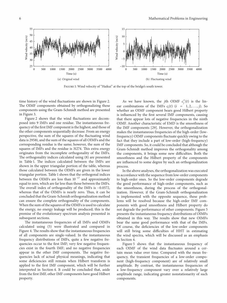
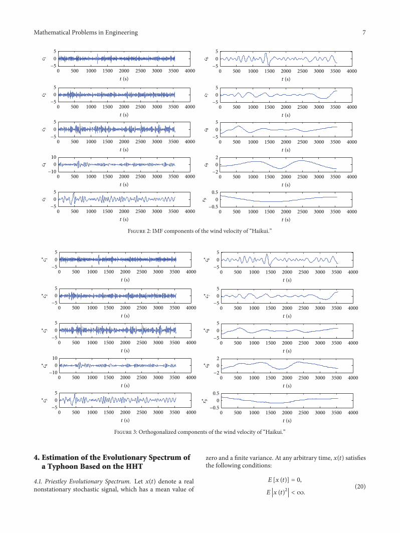
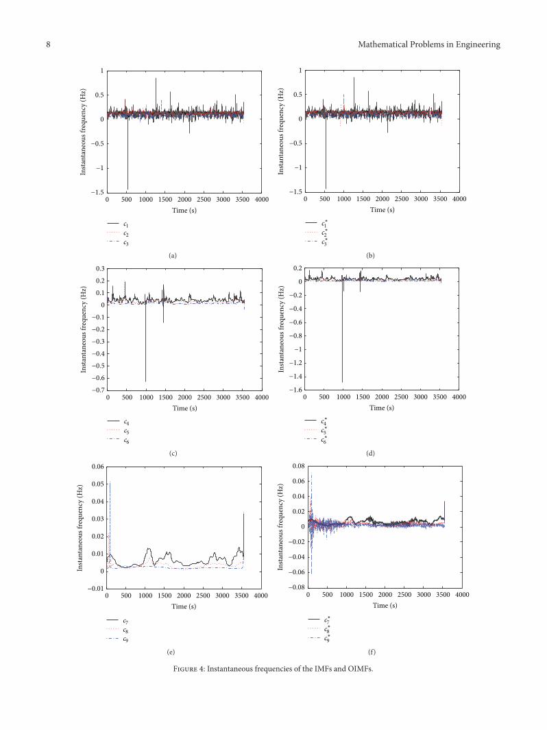
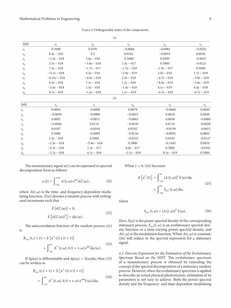
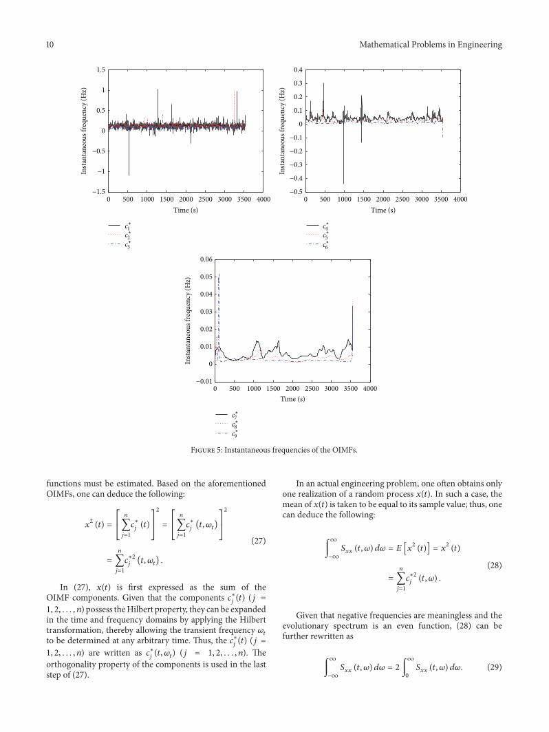
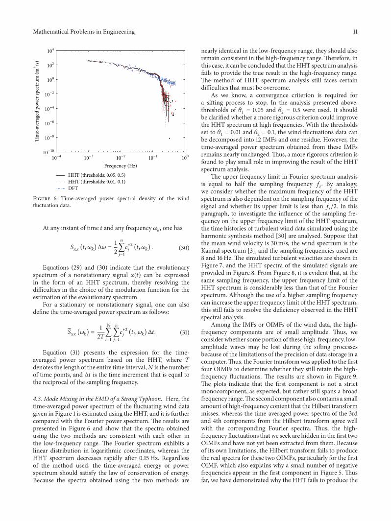
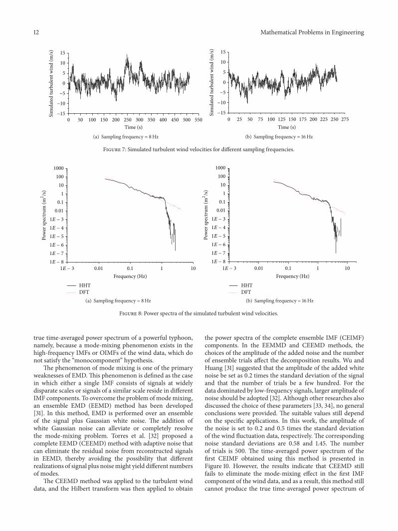
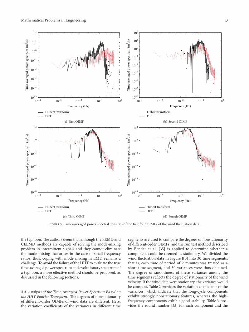
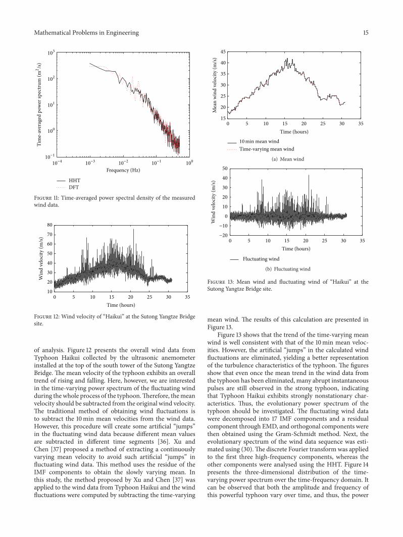
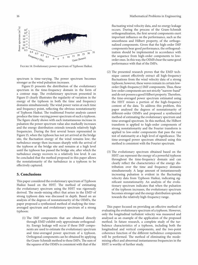
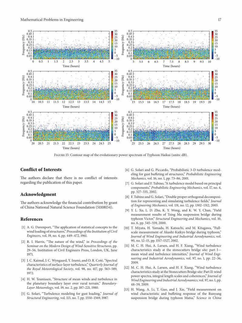formulating a model of a turbulence field based on principalcomponents Tubino and Solari [8] proposed a representationof turbulence based on a double application of the POD

In recent years researchers have performed many fieldmeasurements of the wind characteristics at bridge sites[9ndash15] Using the wind data obtained from the StructuralHealth Monitoring System (SHMS) Xu et al [9] studied themean and turbulent wind characteristics of Typhoon Victorat the site of the Tsing Ma Bridge in Hong Kong It wasfound that certain features of the wind structure and bridgeresponse were difficult to consider in the analytical processthat is currently used to predict the buffeting response oflong suspension bridges as the bridge is surrounded by acomplex topography and the wind direction of TyphoonVictor varied during its passage Miyata et al [10] analysedfull-scale measurement data observed on the Akashi-KaikyoBridge during strong typhoons The power spectral densityand spatial correlation of the longitudinal velocity fluctu-ations were analysed These authors found that the spatialcorrelation of two points was well represented not by anexponential formula but rather by an alternative coherencefunction based on isotropic turbulence theory To derivea model of turbulence suitable for buffeting calculationsregarding the Stonecutters Bridge in Hong Kong Hui et al[11 12] studied the mean wind turbulence intensities windpower spectra integral length scales and wind coherences ofthe bridge

Using statistical theory Wang et al [13] analysed thestrong wind characteristics of Typhoon Matsa the buffetingresponse characteristics of the cable and deck of the RunyangYangtze Bridge and the variation in the buffeting responseRMS versus the wind speedThe results obtained in this studyserved to validate the credibility of current techniques inbuffeting response analysis theory Based on field measure-ments of Typhoon Nuri at the Macao Friendship Bridge siteSong et al [14] proposed that the value of the integral scaleincreased when the eye wall of Typhoon Nuri passed overthe field measurement site In the eye wall of the typhoonthe horizontal spatial correlation was relatively strong andthe horizontal spatial correlation spectrum decayed slowlywith increasing frequency Liu et al [15] compared the windcharacteristics of typhoons and strong monsoons at the siteof the Xi-Hou-Men Bridge The similarities and differencesof wind characteristics between typhoons and monsoonswere analysed Wang et al [16] analysed the recorded real-time wind data measured at the Sutong Yangtze Bridge sitein detail to generate the wind-rose diagram mean windspeed and direction turbulence intensity turbulence integralscale and power spectral density and conducted comparativeanalyses among the inhomogeneous wind characteristics ofthree strong wind events including the Northern windTyphoon Kalmaegi and Typhoon Fung-Wong Wang et al[17] analysed the buffeting responses of the cable-stayedSutong Bridge with the wind spectra used in the design phaseand those obtained experimentally from a long-term SHMsystem to compare the actual buffeting response with designpredictions

In previous studies the Fourier transform has often beenused to obtain wind spectrum information based on the

assumption of stationarity However several studies haveshown that powerful typhoons exhibit strongly nonstationarycharacteristics and that lots of abrupt instantaneous pulsesoccur in strong typhoons Therefore to accurately describethe nonstationary characteristics of powerful typhoons it isnecessary to study their evolutionary power spectra [18]

Because of the limitations of theory it is difficult touse the Fourier transform to analyse a nonstationary signalFirst Fourier theory defines harmonic components over alltime and each frequency exists in a complete harmonicform in the time domain thus many additional harmoniccomponents are required to simulate uneven nonstationarydata which may induce false harmonic components andenergy divergence Second the Fourier transform lacks thecapability of simultaneous positioning in both the time andfrequency domains The spectral analysis results obtainedusing the Fourier transform represent the time-averagedspectral distribution Finally the time resolution and fre-quency resolution of a signal are related to each other and theFourier transform fails to automatically adjust the resolutionsin the time and frequency domains depending on the signalcharacteristics

To address the inadequacy of Fourier analysis researchershave proposed time-frequency analysis methods in whicha time-frequency transform is applied to expand the signalenergy in the time-frequency plane to reflect the process ofvariation of a signal in the time and frequency domainsSuch a time-frequency analysis can describe the changingregularity of a signalrsquos spectrum over time Commonly usedtime-frequency analysis methods include the short-timeFourier transform (STFT) the Winger-Ville distribution thewavelet transform and the Hilbert-Huang transform (HHT)

Huang et al [19] proposed a revolutionary method ofsignal decomposition called empirical mode decomposition(EMD) The EMD components possess the Hilbert propertythat is a time-frequency distribution of these componentsthat bears an actual physical meaning can be obtained byapplying the Hilbert transformTheUSNational Aeronauticsand Space Administration refers to this new time-frequencyanalysis method as the HHT The essence of the method isto decompose an original signal into its different fluctuationsand trends at different scales thereby obtaining a series ofdata with different size characteristics

Although researchers havemade considerable progress inthe field of time-frequency analysis the amplitude spectrumobtained via the direct wavelet transform or the HHT has acompletely different mathematical definition from and offersno quantitative comparability with the traditional Fourierspectrum It is difficult to explain the physical meaning of theamplitude spectrum obtained via a wavelet transform or theHHT Priestley [20] proposed the concept of an evolutionaryspectrum by generalizing the power spectrum of a stationaryrandom process The evolutionary spectrum as a conceptualextension of the power spectrum of a stationary randomprocess can accurately describe the changing characteristicsof a spectrum over time The evolutionary spectrum at anyinstant of time has the same physical significance as thepower spectrum of a stationary random process Thereforethe evolutionary spectrum is considered to possess a good










119910 (119905) =

1

120587

119875int

infin

minusinfin

119909 (120591)

119905 minus 120591

119889120591 (1)


obtained

119911 (119905) = 119909 (119905) + 119894119910 (119905) (2)


119911 (119905) = 119886 (119905) 119890119894120579(119905)

(3)

where

119886 (119905) = [1199092

(119905) + 1199102

(119905)]

12

120579 (119905) = arctan [119910 (119905)

119909 (119905)

]

(4)


120596 (119905) =

119889120579 (119905)

119889119905

(5)





119909 (119905) =

119899

sum

119895=1

119862119895(119905) + 119903

119899(119905) (6)





1and 120579






1= 005 and 120579

2= 10120579

1



119883(119905) = Re[

[

119899

sum

119895

119886119895(119905) 119890119894 int 120596119895(119905)119889119905]

]

(7)






119868119874119879=

sum119899+1

119895=1sum119899+1

119896=1119896 =119895int

119879

0

119888119895(119905) 119888119896(119905) 119889119905

int

119879

0

1198832(119905) 119889119905


=

sum119899+1

119895=1sum119899+1

119896=1119896 =119895sum119873

119894=1119888119895119894119888119896119894

sum119873

119894=11198832

119894

(8)

119868119874119895119896=

int

119879

0

119888119895(119905) 119888119896(119905) 119889119905

[int

119879

0

1198882

119895(119905) 119889119905 + int

119879

0

1198882

119896(119905) 119889119905]

=

sum119873

119894=1119888119895119894119888119896119894

sum119873

119894=1(1198882

119895119894+ 1198882

119896119894)

(9)

where 119868119874119879

and 119868119874119895119896




119899(119905) In addition 119888

1(119905) 1198882(119905) 119888

119899(119905) are used


1(119905) =




1(119905) To obtain


1(119905) from 119888

2(119905)

1198882(119905) = 119888

2(119905) minus 120573

211198881(119905) (10)


21


1(119905)




1(119905)


int

119879

0

1198882(119905) 1198881(119905) 119889119905 = int

119879

0

1198882(119905) 1198881(119905) 119889119905 minus 120573

21int

119879

0

1198882

1(119905) 119889119905

= 0

(11)

12057321=

int

119879

0

1198882(119905) 1198881(119905) 119889119905

int

119879

0

1198882

1(119905) 119889119905

(12)


12057321=

1198882 1198881119879

1198881 1198881119879=

sum119873

119894=111988821198941198881119894

sum119873

119894=11198882

1119894

(13)


119888119895+1(119905) = 119888

119895+1(119905) minus

119895

sum

119894=1

120573119895+1119894

119888119894(119905) (14)




int

119879

0

119888119895+1(119905) 119888119896(119905) 119889119905 = int

119879

0

119888119895+1(119905) 119888119896(119905) 119889119905

minus

119895

sum

119894=1

120573119895+1119894

int

119879

0

119888119894(119905) 119888119896(119905) 119889119905 = 0

(15)


119894(119905) (119894 =


as follows

120573119895+1119896

=

int

119879

0

119888119895+1(119905) 119888119896(119905) 119889119905

int

119879

0

1198882

119896(119905) 119889119905

(16)


120573119895+1119896

=

119888119895+1 119888119896119879

119888119896 119888119896119879=

sum119873

119898=1119888119895+1119898

119888119896119898

sum119873

119898=11198882

119896119898

(17)


119909 (119905) =

119899

sum

119895=1

119888119895(119905) + 119903

119899(119905) =

119899

sum

119895=1

119895

sum

119894=1

120573119895119894119888119894(119905) + 119903

119899(119905)

=

119899

sum

119894=1

119886119894119888119894(119905) + 119903

119899(119905) =

119899

sum

119894=1

119888lowast

119894(119905) + 119903

119899(119905)

(18)

where

119888lowast

119894(119905) = 119886

119894119888119894(119905) (119894 = 1 2 119899)

119886119894=

119899

sum

119895=119894

120573119895119894

(119894 = 1 2 119899) 120573119895119894= 1 (119895 = 119894)

(19)




119894(119905) (119894 = 1 2 119899) and the residue 119903

119899(119905)



0 500 1000 1500 2000 2500 3000 3500 400025

30

35

40

45

50

55

Time (s)

Win

d ve

loci

ty (m

s)

(a) Original wind

0 500 1000 1500 2000 2500 3000 3500 4000minus10

minus5

0

5

10

15

Time (s)

Win

d ve

loci

ty (m

s)







119895(119905) is the lin-






0 500 1000 1500 2000 2500 3000 3500 4000minus5

05

t (s)

0 500 1000 1500 2000 2500 3000 3500 4000minus5

05

t (s)

0 500 1000 1500 2000 2500 3000 3500 4000minus5

05

t (s)

0 500 1000 1500 2000 2500 3000 3500 4000minus10

010

t (s)

0 500 1000 1500 2000 2500 3000 3500 4000minus5

05

t (s)

0 500 1000 1500 2000 2500 3000 3500 4000minus5

05

t (s)

0 500 1000 1500 2000 2500 3000 3500 4000minus5

05

t (s)

0 500 1000 1500 2000 2500 3000 3500 4000minus5

05

t (s)

0 500 1000 1500 2000 2500 3000 3500 4000minus2

02

t (s)

0 500 1000 1500 2000 2500 3000 3500 4000minus05

005

t (s)

r9

c 1c 2

c 3c 4

c 5

c 6c 7

c 8c 9


0 500 1000 1500 2000 2500 3000 3500 4000

05

t (s)

0 500 1000 1500 2000 2500 3000 3500 4000minus5

05

t (s)

0 500 1000 1500 2000 2500 3000 3500 4000minus5

05

t (s)

0 500 1000 1500 2000 2500 3000 3500 4000minus10

010

t (s)

0 500 1000 1500 2000 2500 3000 3500 4000minus5

05

t (s)

0 500 1000 1500 2000 2500 3000 3500 4000minus5

05

t (s)

0 500 1000 1500 2000 2500 3000 3500 4000minus5

05

t (s)

0 500 1000 1500 2000 2500 3000 3500 4000minus5

05

t (s)

0 500 1000 1500 2000 2500 3000 3500 4000minus2

02

t (s)

0 500 1000 1500 2000 2500 3000 3500 4000minus05

005

t (s)

minus5

clowast 1

clowast 2

clowast 3

clowast 4

clowast 5

clowast 6

clowast 7

clowast 8

clowast 9

rlowast 9





119864 [119909 (119905)] = 0

119864

10038161003816100381610038161003816119909 (119905)210038161003816100381610038161003816lt infin

(20)


0 500 1000 1500 2000 2500 3000 3500 4000minus15

minus1

minus05

0

05

1

Time (s)

Inst

anta

neou

s fre

quen

cy (H

z)

c1

c2

c3

(a)

0 500 1000 1500 2000 2500 3000 3500 4000minus15

minus1

minus05

0

05

1

Time (s)

Inst

anta

neou

s fre

quen

cy (H

z)

clowast

1

clowast

2

clowast

3

(b)


0010203

Time (s)

Inst

anta

neou

s fre

quen

cy (H

z)

c4

c5

c6

(c)

0 500 1000 1500 2000 2500 3000 3500 4000minus16

minus14

minus12

minus1

minus08

minus06

minus04

minus02

0

02

Time (s)

Inst

anta

neou

s fre

quen

cy (H

z)

clowast

4

clowast

5

clowast

6

(d)

0 500 1000 1500 2000 2500 3000 3500 4000minus001

0

001

002

003

004

005

006

Time (s)

Inst

anta

neou

s fre

quen

cy (H

z)

c7

c8

c9

(e)

0 500 1000 1500 2000 2500 3000 3500 4000minus008

minus006

minus004

minus002

0

002

004

006

008

Time (s)

Inst

anta

neou

s fre

quen

cy (H

z)

clowast

7

clowast

8

clowast

9

(f)




(a)

IMF 1198881

1198882

1198883

1198884

1198885

1198881


1198882

84119890 minus 018 05 00161 minus00055 00026

1198883


1198884


1198885


1198886


1198887


1198888


1198889


1199039


(b)

IMF 1198886

1198887

1198888

1198889

1199039

1198881

00004 minus00008 00079 minus00068 00000

1198882


1198883


1198884


1198885


1198886


1198887


1198888


1198889


1199039



119909 (119905) = int

+infin

minusinfin

119860 (119905 120596) 119890119894120596119905

119889119885 (120596) (21)


119864 [119889119885 (120596)] = 0

119864 [|119889119885 (120596)|2

] = 119889120583 (120596)

(22)


119877119909119909(119905 119905 + 120591) = 119864 [119909

lowast

(119905) 119909 (119905 + 120591)]

= int

infin

minusinfin

119860lowast

(119905 120596) 119860 (119905 + 120591 120596) 119890119894120596119905

119889120583 (120596)

(23)


119877119909119909(119905 119905 + 120591) = 119864 [119909

lowast

(119905) 119909 (119905 + 120591)]

= int

infin

minusinfin

119860lowast

(119905 120596) 119860 (119905 + 120591 120596) 119890119894120596119905

119878 (120596) 119889120596

(24)

When 120591 = 0 (24) becomes

119864 [1199092

(119905)] = int

infin

minusinfin

|119860 (119905 120596)|2

119878 (120596) 119889120596

= int

infin

minusinfin

119878119909119909(119905 120596) 119889120596

(25)

where

119878119909119909(119905 120596) = |119860 (119905 120596)|

2

119878 (120596) (26)






0 500 1000 1500 2000 2500 3000 3500 4000minus15

minus1

minus05

0

05

1

15

Time (s)

Inst

anta

neou

s fre

quen

cy (H

z)

0 500 1000 1500 2000 2500 3000 3500 4000minus05

minus04

minus03

minus02

minus01

0

01

02

03

04

Time (s)

Inst

anta

neou

s fre

quen

cy (H

z)

0 500 1000 1500 2000 2500 3000 3500 4000minus001

0

001

002

003

004

005

006

Time (s)

Inst

anta

neou

s fre

quen

cy (H

z)

clowast

4

clowast

5

clowast

6

clowast

1

clowast

2

clowast

3

clowast

7

clowast

8

clowast

9



1199092

(119905) =[

[

119899

sum

119895=1

119888lowast

119895(119905)]

]

2

=[

[

119899

sum

119895=1

119888lowast

119895(119905 120596119905)]

]

2

=

119899

sum

119895=1

119888lowast2

119895(119905 120596119905)

(27)


119895(119905) (119895 =


119905





int

infin

minusinfin

119878119909119909(119905 120596) 119889120596 = 119864 [119909

2

(119905)] = 1199092

(119905)

=

119899

sum

119895=1

119888lowast2

119895(119905 120596)

(28)


int

infin

minusinfin

119878119909119909(119905 120596) 119889120596 = 2int

infin

0

119878119909119909(119905 120596) 119889120596 (29)


Frequency (Hz)

Tim

e-av

erag

ed p

ower

spec

trum

(m2s

)

104

102

100

100

10minus2

10minus4

10minus4

10minus3

10minus2

10minus1

10minus6

10minus8

10minus10




119878119909119909(119905 120596119896) Δ120596 =

1

2

119899

sum

119895=1

119888lowast2

119895(119905 120596119896) (30)



119878119909119909(120596119896) =

1

2119879

119873

sum

119894=1

119899

sum

119895=1

119888lowast2

119895(119905119894 120596119896) Δ119905 (31)





1= 005 and 120579



1= 001 and 120579




119904 By analogy


1199042 In this




0 50 100 150 200 250 300 350 400 450 500 550minus15

minus10

minus5

0

5

10

15Si

mul

ated

turb

ulen

t win

d (m

s)

Time (s)


0 25 50 75 100 125 150 175 200 225 250 275minus15

minus10

minus5

0

5

10

15

Sim

ulat

ed tu

rbul

ent w

ind

(ms

)

Time (s)



001 01 1 10

00101

110

1001000

Frequency (Hz)

Pow

er sp

ectr

um (m

2s

)

1E minus 3

1E minus 3

1E minus 4

1E minus 5

1E minus 6

1E minus 7

1E minus 8

HHTDFT



00101

110

1001000

Pow

er sp

ectr

um (m

2s

)

1E minus 3

1E minus 3

1E minus 4

1E minus 5

1E minus 6

1E minus 7

1E minus 8








Frequency (Hz)

Tim

e-av

erag

ed p

ower

spec

trum

(m2s

)

100

10minus4

10minus3

10minus2

10minus1

102

101

100

10minus1

10minus2

10minus3

10minus4

10minus5


(a) First OIMF

Frequency (Hz)

Tim

e-av

erag

ed p

ower

spec

trum

(m2s

)

100

10minus4

10minus3

10minus2

10minus1

102

101

100

10minus1

10minus2

10minus3

10minus4

10minus5

10minus6


(b) Second OIMF

Frequency (Hz)

Tim

e-av

erag

ed p

ower

spec

trum

(m2s

)

100

10minus4

10minus3

10minus2

10minus1

102

100

10minus2

10minus4

10minus6

10minus8


(c) Third OIMF

Frequency (Hz)

Tim

e-av

erag

ed p

ower

spec

trum

(m2s

)10

2

100

100

10minus2

10minus4

10minus4

10minus3

10minus2

10minus1

10minus6

10minus8


(d) Fourth OIMF






Frequency (Hz)

Tim

e-av

erag

ed p

ower

spec

trum

(m2s

)

102

100

100

10minus2

10minus4

10minus4

10minus3

10minus2

10minus1

10minus6

10minus8



Frequency (Hz)

Tim

e-av

erag

ed p

ower

spec

trum

(m2s

)

102

100

100

10minus2

10minus4

10minus4

10minus3

10minus2

10minus1

10minus6

10minus8





026011198882

052201198883

061931198884

094821198885

106161198886

109791198887

118921198888

133001198889

110701199039

08872



15 [11 20]

1198882

18 [11 20]

1198883

16 [11 20]

1198884

14 [11 20]

1198885

15 [11 20]

1198886

9 [11 20]

1198887

11 [11 20]

1198888

8 [11 20]

1198889

11 [11 20]

1199039

15 [11 20]






Frequency (Hz)

Tim

e-av

erag

ed p

ower

spec

trum

(m2s

)

101

102

103

100

100

10minus1

10minus4

10minus3

10minus2

10minus1

HHTDFT


0 5 10 15 20 25 30 3510

20

30

40

50

60

70

80

Time (hours)

Win

d ve

loci

ty (m

s)



0 5 10 15 20 25 30 3515

20

25

30

35

40

45

Time (hours)

Mea

n w

ind

velo

city

(ms

)


(a) Mean wind

0 5 10 15 20 25 30 35minus20

minus10

0

10

20

30

40

50

Time (hours)

Win

d ve

loci

ty (m

s)

Fluctuating wind






0 5 10 15 20 25 30 35

00102030405


102

100

10minus2

10minus4

10minus6

10minus8

10minus10

Pow

er sp

ectr

um (m

2s

)




5 Conclusions








05

045

04

035

03

025

02

015

01

005

0

20 205 21 215 22 225 23 235 24 245 25 25 255 26 265 27 275 28 285 29 295 30

05

045

04

035

03

025

02

015

01

005

0

35

30

25

20

15

10

5

0

minus5

minus10

35

30

25

20

15

10

5

0

minus5

minus10

10 105 11 115 12 125 13 135 14 145 15 15 155 16 165 17 175 18 185 19 195 20

05

045

04

035

03

025

02

015

01

005

0

05

045

04

035

03

025

02

015

01

005

0

35

30

25

20

15

10

5

0

minus5

minus10

35

30

25

20

15

10

5

0

minus5

minus10

35

30

25

20

15

10

5

0

minus5

minus100 05 1 15 2 25 3 35 4 45 5 5 55 6 65 7 75 8 85 9 95 10

05

045

04

035

03

025

02

015

01

005

0

05

045

04

035

03

025

02

015

01

005

0

35

30

25

20

15

10

5

0

minus5

minus10

Freq

uenc

y (H

z)Fr

eque

ncy

(Hz)

Freq

uenc

y (H

z)

Freq

uenc

y (H

z)Fr

eque

ncy

(Hz)

Freq

uenc

y (H

z)







Acknowledgment


References















































Volume 2014




Journal of











Journal of


Function Spaces






Algebra


















119910 (119905) =

1

120587

119875int

infin

minusinfin

119909 (120591)

119905 minus 120591

119889120591 (1)


obtained

119911 (119905) = 119909 (119905) + 119894119910 (119905) (2)


119911 (119905) = 119886 (119905) 119890119894120579(119905)

(3)

where

119886 (119905) = [1199092

(119905) + 1199102

(119905)]

12

120579 (119905) = arctan [119910 (119905)

119909 (119905)

]

(4)


120596 (119905) =

119889120579 (119905)

119889119905

(5)





119909 (119905) =

119899

sum

119895=1

119862119895(119905) + 119903

119899(119905) (6)





1and 120579






1= 005 and 120579

2= 10120579

1



119883(119905) = Re[

[

119899

sum

119895

119886119895(119905) 119890119894 int 120596119895(119905)119889119905]

]

(7)






119868119874119879=

sum119899+1

119895=1sum119899+1

119896=1119896 =119895int

119879

0

119888119895(119905) 119888119896(119905) 119889119905

int

119879

0

1198832(119905) 119889119905


=

sum119899+1

119895=1sum119899+1

119896=1119896 =119895sum119873

119894=1119888119895119894119888119896119894

sum119873

119894=11198832

119894

(8)

119868119874119895119896=

int

119879

0

119888119895(119905) 119888119896(119905) 119889119905

[int

119879

0

1198882

119895(119905) 119889119905 + int

119879

0

1198882

119896(119905) 119889119905]

=

sum119873

119894=1119888119895119894119888119896119894

sum119873

119894=1(1198882

119895119894+ 1198882

119896119894)

(9)

where 119868119874119879

and 119868119874119895119896




119899(119905) In addition 119888

1(119905) 1198882(119905) 119888

119899(119905) are used


1(119905) =




1(119905) To obtain


1(119905) from 119888

2(119905)

1198882(119905) = 119888

2(119905) minus 120573

211198881(119905) (10)


21


1(119905)




1(119905)


int

119879

0

1198882(119905) 1198881(119905) 119889119905 = int

119879

0

1198882(119905) 1198881(119905) 119889119905 minus 120573

21int

119879

0

1198882

1(119905) 119889119905

= 0

(11)

12057321=

int

119879

0

1198882(119905) 1198881(119905) 119889119905

int

119879

0

1198882

1(119905) 119889119905

(12)


12057321=

1198882 1198881119879

1198881 1198881119879=

sum119873

119894=111988821198941198881119894

sum119873

119894=11198882

1119894

(13)


119888119895+1(119905) = 119888

119895+1(119905) minus

119895

sum

119894=1

120573119895+1119894

119888119894(119905) (14)




int

119879

0

119888119895+1(119905) 119888119896(119905) 119889119905 = int

119879

0

119888119895+1(119905) 119888119896(119905) 119889119905

minus

119895

sum

119894=1

120573119895+1119894

int

119879

0

119888119894(119905) 119888119896(119905) 119889119905 = 0

(15)


119894(119905) (119894 =


as follows

120573119895+1119896

=

int

119879

0

119888119895+1(119905) 119888119896(119905) 119889119905

int

119879

0

1198882

119896(119905) 119889119905

(16)


120573119895+1119896

=

119888119895+1 119888119896119879

119888119896 119888119896119879=

sum119873

119898=1119888119895+1119898

119888119896119898

sum119873

119898=11198882

119896119898

(17)


119909 (119905) =

119899

sum

119895=1

119888119895(119905) + 119903

119899(119905) =

119899

sum

119895=1

119895

sum

119894=1

120573119895119894119888119894(119905) + 119903

119899(119905)

=

119899

sum

119894=1

119886119894119888119894(119905) + 119903

119899(119905) =

119899

sum

119894=1

119888lowast

119894(119905) + 119903

119899(119905)

(18)

where

119888lowast

119894(119905) = 119886

119894119888119894(119905) (119894 = 1 2 119899)

119886119894=

119899

sum

119895=119894

120573119895119894

(119894 = 1 2 119899) 120573119895119894= 1 (119895 = 119894)

(19)




119894(119905) (119894 = 1 2 119899) and the residue 119903

119899(119905)



0 500 1000 1500 2000 2500 3000 3500 400025

30

35

40

45

50

55

Time (s)

Win

d ve

loci

ty (m

s)

(a) Original wind

0 500 1000 1500 2000 2500 3000 3500 4000minus10

minus5

0

5

10

15

Time (s)

Win

d ve

loci

ty (m

s)







119895(119905) is the lin-






0 500 1000 1500 2000 2500 3000 3500 4000minus5

05

t (s)

0 500 1000 1500 2000 2500 3000 3500 4000minus5

05

t (s)

0 500 1000 1500 2000 2500 3000 3500 4000minus5

05

t (s)

0 500 1000 1500 2000 2500 3000 3500 4000minus10

010

t (s)

0 500 1000 1500 2000 2500 3000 3500 4000minus5

05

t (s)

0 500 1000 1500 2000 2500 3000 3500 4000minus5

05

t (s)

0 500 1000 1500 2000 2500 3000 3500 4000minus5

05

t (s)

0 500 1000 1500 2000 2500 3000 3500 4000minus5

05

t (s)

0 500 1000 1500 2000 2500 3000 3500 4000minus2

02

t (s)

0 500 1000 1500 2000 2500 3000 3500 4000minus05

005

t (s)

r9

c 1c 2

c 3c 4

c 5

c 6c 7

c 8c 9


0 500 1000 1500 2000 2500 3000 3500 4000

05

t (s)

0 500 1000 1500 2000 2500 3000 3500 4000minus5

05

t (s)

0 500 1000 1500 2000 2500 3000 3500 4000minus5

05

t (s)

0 500 1000 1500 2000 2500 3000 3500 4000minus10

010

t (s)

0 500 1000 1500 2000 2500 3000 3500 4000minus5

05

t (s)

0 500 1000 1500 2000 2500 3000 3500 4000minus5

05

t (s)

0 500 1000 1500 2000 2500 3000 3500 4000minus5

05

t (s)

0 500 1000 1500 2000 2500 3000 3500 4000minus5

05

t (s)

0 500 1000 1500 2000 2500 3000 3500 4000minus2

02

t (s)

0 500 1000 1500 2000 2500 3000 3500 4000minus05

005

t (s)

minus5

clowast 1

clowast 2

clowast 3

clowast 4

clowast 5

clowast 6

clowast 7

clowast 8

clowast 9

rlowast 9





119864 [119909 (119905)] = 0

119864

10038161003816100381610038161003816119909 (119905)210038161003816100381610038161003816lt infin

(20)


0 500 1000 1500 2000 2500 3000 3500 4000minus15

minus1

minus05

0

05

1

Time (s)

Inst

anta

neou

s fre

quen

cy (H

z)

c1

c2

c3

(a)

0 500 1000 1500 2000 2500 3000 3500 4000minus15

minus1

minus05

0

05

1

Time (s)

Inst

anta

neou

s fre

quen

cy (H

z)

clowast

1

clowast

2

clowast

3

(b)


0010203

Time (s)

Inst

anta

neou

s fre

quen

cy (H

z)

c4

c5

c6

(c)

0 500 1000 1500 2000 2500 3000 3500 4000minus16

minus14

minus12

minus1

minus08

minus06

minus04

minus02

0

02

Time (s)

Inst

anta

neou

s fre

quen

cy (H

z)

clowast

4

clowast

5

clowast

6

(d)

0 500 1000 1500 2000 2500 3000 3500 4000minus001

0

001

002

003

004

005

006

Time (s)

Inst

anta

neou

s fre

quen

cy (H

z)

c7

c8

c9

(e)

0 500 1000 1500 2000 2500 3000 3500 4000minus008

minus006

minus004

minus002

0

002

004

006

008

Time (s)

Inst

anta

neou

s fre

quen

cy (H

z)

clowast

7

clowast

8

clowast

9

(f)




(a)

IMF 1198881

1198882

1198883

1198884

1198885

1198881


1198882

84119890 minus 018 05 00161 minus00055 00026

1198883


1198884


1198885


1198886


1198887


1198888


1198889


1199039


(b)

IMF 1198886

1198887

1198888

1198889

1199039

1198881

00004 minus00008 00079 minus00068 00000

1198882


1198883


1198884


1198885


1198886


1198887


1198888


1198889


1199039



119909 (119905) = int

+infin

minusinfin

119860 (119905 120596) 119890119894120596119905

119889119885 (120596) (21)


119864 [119889119885 (120596)] = 0

119864 [|119889119885 (120596)|2

] = 119889120583 (120596)

(22)


119877119909119909(119905 119905 + 120591) = 119864 [119909

lowast

(119905) 119909 (119905 + 120591)]

= int

infin

minusinfin

119860lowast

(119905 120596) 119860 (119905 + 120591 120596) 119890119894120596119905

119889120583 (120596)

(23)


119877119909119909(119905 119905 + 120591) = 119864 [119909

lowast

(119905) 119909 (119905 + 120591)]

= int

infin

minusinfin

119860lowast

(119905 120596) 119860 (119905 + 120591 120596) 119890119894120596119905

119878 (120596) 119889120596

(24)

When 120591 = 0 (24) becomes

119864 [1199092

(119905)] = int

infin

minusinfin

|119860 (119905 120596)|2

119878 (120596) 119889120596

= int

infin

minusinfin

119878119909119909(119905 120596) 119889120596

(25)

where

119878119909119909(119905 120596) = |119860 (119905 120596)|

2

119878 (120596) (26)






0 500 1000 1500 2000 2500 3000 3500 4000minus15

minus1

minus05

0

05

1

15

Time (s)

Inst

anta

neou

s fre

quen

cy (H

z)

0 500 1000 1500 2000 2500 3000 3500 4000minus05

minus04

minus03

minus02

minus01

0

01

02

03

04

Time (s)

Inst

anta

neou

s fre

quen

cy (H

z)

0 500 1000 1500 2000 2500 3000 3500 4000minus001

0

001

002

003

004

005

006

Time (s)

Inst

anta

neou

s fre

quen

cy (H

z)

clowast

4

clowast

5

clowast

6

clowast

1

clowast

2

clowast

3

clowast

7

clowast

8

clowast

9



1199092

(119905) =[

[

119899

sum

119895=1

119888lowast

119895(119905)]

]

2

=[

[

119899

sum

119895=1

119888lowast

119895(119905 120596119905)]

]

2

=

119899

sum

119895=1

119888lowast2

119895(119905 120596119905)

(27)


119895(119905) (119895 =


119905





int

infin

minusinfin

119878119909119909(119905 120596) 119889120596 = 119864 [119909

2

(119905)] = 1199092

(119905)

=

119899

sum

119895=1

119888lowast2

119895(119905 120596)

(28)


int

infin

minusinfin

119878119909119909(119905 120596) 119889120596 = 2int

infin

0

119878119909119909(119905 120596) 119889120596 (29)


Frequency (Hz)

Tim

e-av

erag

ed p

ower

spec

trum

(m2s

)

104

102

100

100

10minus2

10minus4

10minus4

10minus3

10minus2

10minus1

10minus6

10minus8

10minus10




119878119909119909(119905 120596119896) Δ120596 =

1

2

119899

sum

119895=1

119888lowast2

119895(119905 120596119896) (30)



119878119909119909(120596119896) =

1

2119879

119873

sum

119894=1

119899

sum

119895=1

119888lowast2

119895(119905119894 120596119896) Δ119905 (31)





1= 005 and 120579



1= 001 and 120579




119904 By analogy


1199042 In this




0 50 100 150 200 250 300 350 400 450 500 550minus15

minus10

minus5

0

5

10

15Si

mul

ated

turb

ulen

t win

d (m

s)

Time (s)


0 25 50 75 100 125 150 175 200 225 250 275minus15

minus10

minus5

0

5

10

15

Sim

ulat

ed tu

rbul

ent w

ind

(ms

)

Time (s)



001 01 1 10

00101

110

1001000

Frequency (Hz)

Pow

er sp

ectr

um (m

2s

)

1E minus 3

1E minus 3

1E minus 4

1E minus 5

1E minus 6

1E minus 7

1E minus 8

HHTDFT



00101

110

1001000

Pow

er sp

ectr

um (m

2s

)

1E minus 3

1E minus 3

1E minus 4

1E minus 5

1E minus 6

1E minus 7

1E minus 8








Frequency (Hz)

Tim

e-av

erag

ed p

ower

spec

trum

(m2s

)

100

10minus4

10minus3

10minus2

10minus1

102

101

100

10minus1

10minus2

10minus3

10minus4

10minus5


(a) First OIMF

Frequency (Hz)

Tim

e-av

erag

ed p

ower

spec

trum

(m2s

)

100

10minus4

10minus3

10minus2

10minus1

102

101

100

10minus1

10minus2

10minus3

10minus4

10minus5

10minus6


(b) Second OIMF

Frequency (Hz)

Tim

e-av

erag

ed p

ower

spec

trum

(m2s

)

100

10minus4

10minus3

10minus2

10minus1

102

100

10minus2

10minus4

10minus6

10minus8


(c) Third OIMF

Frequency (Hz)

Tim

e-av

erag

ed p

ower

spec

trum

(m2s

)10

2

100

100

10minus2

10minus4

10minus4

10minus3

10minus2

10minus1

10minus6

10minus8


(d) Fourth OIMF






Frequency (Hz)

Tim

e-av

erag

ed p

ower

spec

trum

(m2s

)

102

100

100

10minus2

10minus4

10minus4

10minus3

10minus2

10minus1

10minus6

10minus8



Frequency (Hz)

Tim

e-av

erag

ed p

ower

spec

trum

(m2s

)

102

100

100

10minus2

10minus4

10minus4

10minus3

10minus2

10minus1

10minus6

10minus8





026011198882

052201198883

061931198884

094821198885

106161198886

109791198887

118921198888

133001198889

110701199039

08872



15 [11 20]

1198882

18 [11 20]

1198883

16 [11 20]

1198884

14 [11 20]

1198885

15 [11 20]

1198886

9 [11 20]

1198887

11 [11 20]

1198888

8 [11 20]

1198889

11 [11 20]

1199039

15 [11 20]






Frequency (Hz)

Tim

e-av

erag

ed p

ower

spec

trum

(m2s

)

101

102

103

100

100

10minus1

10minus4

10minus3

10minus2

10minus1

HHTDFT


0 5 10 15 20 25 30 3510

20

30

40

50

60

70

80

Time (hours)

Win

d ve

loci

ty (m

s)



0 5 10 15 20 25 30 3515

20

25

30

35

40

45

Time (hours)

Mea

n w

ind

velo

city

(ms

)


(a) Mean wind

0 5 10 15 20 25 30 35minus20

minus10

0

10

20

30

40

50

Time (hours)

Win

d ve

loci

ty (m

s)

Fluctuating wind






0 5 10 15 20 25 30 35

00102030405


102

100

10minus2

10minus4

10minus6

10minus8

10minus10

Pow

er sp

ectr

um (m

2s

)




5 Conclusions








05

045

04

035

03

025

02

015

01

005

0

20 205 21 215 22 225 23 235 24 245 25 25 255 26 265 27 275 28 285 29 295 30

05

045

04

035

03

025

02

015

01

005

0

35

30

25

20

15

10

5

0

minus5

minus10

35

30

25

20

15

10

5

0

minus5

minus10

10 105 11 115 12 125 13 135 14 145 15 15 155 16 165 17 175 18 185 19 195 20

05

045

04

035

03

025

02

015

01

005

0

05

045

04

035

03

025

02

015

01

005

0

35

30

25

20

15

10

5

0

minus5

minus10

35

30

25

20

15

10

5

0

minus5

minus10

35

30

25

20

15

10

5

0

minus5

minus100 05 1 15 2 25 3 35 4 45 5 5 55 6 65 7 75 8 85 9 95 10

05

045

04

035

03

025

02

015

01

005

0

05

045

04

035

03

025

02

015

01

005

0

35

30

25

20

15

10

5

0

minus5

minus10

Freq

uenc

y (H

z)Fr

eque

ncy

(Hz)

Freq

uenc

y (H

z)

Freq

uenc

y (H

z)Fr

eque

ncy

(Hz)

Freq

uenc

y (H

z)







Acknowledgment


References















































Volume 2014




Journal of











Journal of


Function Spaces






Algebra












119909 (119905) =

119899

sum

119895=1

119862119895(119905) + 119903

119899(119905) (6)





1and 120579






1= 005 and 120579

2= 10120579

1



119883(119905) = Re[

[

119899

sum

119895

119886119895(119905) 119890119894 int 120596119895(119905)119889119905]

]

(7)






119868119874119879=

sum119899+1

119895=1sum119899+1

119896=1119896 =119895int

119879

0

119888119895(119905) 119888119896(119905) 119889119905

int

119879

0

1198832(119905) 119889119905


=

sum119899+1

119895=1sum119899+1

119896=1119896 =119895sum119873

119894=1119888119895119894119888119896119894

sum119873

119894=11198832

119894

(8)

119868119874119895119896=

int

119879

0

119888119895(119905) 119888119896(119905) 119889119905

[int

119879

0

1198882

119895(119905) 119889119905 + int

119879

0

1198882

119896(119905) 119889119905]

=

sum119873

119894=1119888119895119894119888119896119894

sum119873

119894=1(1198882

119895119894+ 1198882

119896119894)

(9)

where 119868119874119879

and 119868119874119895119896




119899(119905) In addition 119888

1(119905) 1198882(119905) 119888

119899(119905) are used


1(119905) =




1(119905) To obtain


1(119905) from 119888

2(119905)

1198882(119905) = 119888

2(119905) minus 120573

211198881(119905) (10)


21


1(119905)




1(119905)


int

119879

0

1198882(119905) 1198881(119905) 119889119905 = int

119879

0

1198882(119905) 1198881(119905) 119889119905 minus 120573

21int

119879

0

1198882

1(119905) 119889119905

= 0

(11)

12057321=

int

119879

0

1198882(119905) 1198881(119905) 119889119905

int

119879

0

1198882

1(119905) 119889119905

(12)


12057321=

1198882 1198881119879

1198881 1198881119879=

sum119873

119894=111988821198941198881119894

sum119873

119894=11198882

1119894

(13)


119888119895+1(119905) = 119888

119895+1(119905) minus

119895

sum

119894=1

120573119895+1119894

119888119894(119905) (14)




int

119879

0

119888119895+1(119905) 119888119896(119905) 119889119905 = int

119879

0

119888119895+1(119905) 119888119896(119905) 119889119905

minus

119895

sum

119894=1

120573119895+1119894

int

119879

0

119888119894(119905) 119888119896(119905) 119889119905 = 0

(15)


119894(119905) (119894 =


as follows

120573119895+1119896

=

int

119879

0

119888119895+1(119905) 119888119896(119905) 119889119905

int

119879

0

1198882

119896(119905) 119889119905

(16)


120573119895+1119896

=

119888119895+1 119888119896119879

119888119896 119888119896119879=

sum119873

119898=1119888119895+1119898

119888119896119898

sum119873

119898=11198882

119896119898

(17)


119909 (119905) =

119899

sum

119895=1

119888119895(119905) + 119903

119899(119905) =

119899

sum

119895=1

119895

sum

119894=1

120573119895119894119888119894(119905) + 119903

119899(119905)

=

119899

sum

119894=1

119886119894119888119894(119905) + 119903

119899(119905) =

119899

sum

119894=1

119888lowast

119894(119905) + 119903

119899(119905)

(18)

where

119888lowast

119894(119905) = 119886

119894119888119894(119905) (119894 = 1 2 119899)

119886119894=

119899

sum

119895=119894

120573119895119894

(119894 = 1 2 119899) 120573119895119894= 1 (119895 = 119894)

(19)




119894(119905) (119894 = 1 2 119899) and the residue 119903

119899(119905)



0 500 1000 1500 2000 2500 3000 3500 400025

30

35

40

45

50

55

Time (s)

Win

d ve

loci

ty (m

s)

(a) Original wind

0 500 1000 1500 2000 2500 3000 3500 4000minus10

minus5

0

5

10

15

Time (s)

Win

d ve

loci

ty (m

s)







119895(119905) is the lin-






0 500 1000 1500 2000 2500 3000 3500 4000minus5

05

t (s)

0 500 1000 1500 2000 2500 3000 3500 4000minus5

05

t (s)

0 500 1000 1500 2000 2500 3000 3500 4000minus5

05

t (s)

0 500 1000 1500 2000 2500 3000 3500 4000minus10

010

t (s)

0 500 1000 1500 2000 2500 3000 3500 4000minus5

05

t (s)

0 500 1000 1500 2000 2500 3000 3500 4000minus5

05

t (s)

0 500 1000 1500 2000 2500 3000 3500 4000minus5

05

t (s)

0 500 1000 1500 2000 2500 3000 3500 4000minus5

05

t (s)

0 500 1000 1500 2000 2500 3000 3500 4000minus2

02

t (s)

0 500 1000 1500 2000 2500 3000 3500 4000minus05

005

t (s)

r9

c 1c 2

c 3c 4

c 5

c 6c 7

c 8c 9


0 500 1000 1500 2000 2500 3000 3500 4000

05

t (s)

0 500 1000 1500 2000 2500 3000 3500 4000minus5

05

t (s)

0 500 1000 1500 2000 2500 3000 3500 4000minus5

05

t (s)

0 500 1000 1500 2000 2500 3000 3500 4000minus10

010

t (s)

0 500 1000 1500 2000 2500 3000 3500 4000minus5

05

t (s)

0 500 1000 1500 2000 2500 3000 3500 4000minus5

05

t (s)

0 500 1000 1500 2000 2500 3000 3500 4000minus5

05

t (s)

0 500 1000 1500 2000 2500 3000 3500 4000minus5

05

t (s)

0 500 1000 1500 2000 2500 3000 3500 4000minus2

02

t (s)

0 500 1000 1500 2000 2500 3000 3500 4000minus05

005

t (s)

minus5

clowast 1

clowast 2

clowast 3

clowast 4

clowast 5

clowast 6

clowast 7

clowast 8

clowast 9

rlowast 9





119864 [119909 (119905)] = 0

119864

10038161003816100381610038161003816119909 (119905)210038161003816100381610038161003816lt infin

(20)


0 500 1000 1500 2000 2500 3000 3500 4000minus15

minus1

minus05

0

05

1

Time (s)

Inst

anta

neou

s fre

quen

cy (H

z)

c1

c2

c3

(a)

0 500 1000 1500 2000 2500 3000 3500 4000minus15

minus1

minus05

0

05

1

Time (s)

Inst

anta

neou

s fre

quen

cy (H

z)

clowast

1

clowast

2

clowast

3

(b)


0010203

Time (s)

Inst

anta

neou

s fre

quen

cy (H

z)

c4

c5

c6

(c)

0 500 1000 1500 2000 2500 3000 3500 4000minus16

minus14

minus12

minus1

minus08

minus06

minus04

minus02

0

02

Time (s)

Inst

anta

neou

s fre

quen

cy (H

z)

clowast

4

clowast

5

clowast

6

(d)

0 500 1000 1500 2000 2500 3000 3500 4000minus001

0

001

002

003

004

005

006

Time (s)

Inst

anta

neou

s fre

quen

cy (H

z)

c7

c8

c9

(e)

0 500 1000 1500 2000 2500 3000 3500 4000minus008

minus006

minus004

minus002

0

002

004

006

008

Time (s)

Inst

anta

neou

s fre

quen

cy (H

z)

clowast

7

clowast

8

clowast

9

(f)




(a)

IMF 1198881

1198882

1198883

1198884

1198885

1198881


1198882

84119890 minus 018 05 00161 minus00055 00026

1198883


1198884


1198885


1198886


1198887


1198888


1198889


1199039


(b)

IMF 1198886

1198887

1198888

1198889

1199039

1198881

00004 minus00008 00079 minus00068 00000

1198882


1198883


1198884


1198885


1198886


1198887


1198888


1198889


1199039



119909 (119905) = int

+infin

minusinfin

119860 (119905 120596) 119890119894120596119905

119889119885 (120596) (21)


119864 [119889119885 (120596)] = 0

119864 [|119889119885 (120596)|2

] = 119889120583 (120596)

(22)


119877119909119909(119905 119905 + 120591) = 119864 [119909

lowast

(119905) 119909 (119905 + 120591)]

= int

infin

minusinfin

119860lowast

(119905 120596) 119860 (119905 + 120591 120596) 119890119894120596119905

119889120583 (120596)

(23)


119877119909119909(119905 119905 + 120591) = 119864 [119909

lowast

(119905) 119909 (119905 + 120591)]

= int

infin

minusinfin

119860lowast

(119905 120596) 119860 (119905 + 120591 120596) 119890119894120596119905

119878 (120596) 119889120596

(24)

When 120591 = 0 (24) becomes

119864 [1199092

(119905)] = int

infin

minusinfin

|119860 (119905 120596)|2

119878 (120596) 119889120596

= int

infin

minusinfin

119878119909119909(119905 120596) 119889120596

(25)

where

119878119909119909(119905 120596) = |119860 (119905 120596)|

2

119878 (120596) (26)






0 500 1000 1500 2000 2500 3000 3500 4000minus15

minus1

minus05

0

05

1

15

Time (s)

Inst

anta

neou

s fre

quen

cy (H

z)

0 500 1000 1500 2000 2500 3000 3500 4000minus05

minus04

minus03

minus02

minus01

0

01

02

03

04

Time (s)

Inst

anta

neou

s fre

quen

cy (H

z)

0 500 1000 1500 2000 2500 3000 3500 4000minus001

0

001

002

003

004

005

006

Time (s)

Inst

anta

neou

s fre

quen

cy (H

z)

clowast

4

clowast

5

clowast

6

clowast

1

clowast

2

clowast

3

clowast

7

clowast

8

clowast

9



1199092

(119905) =[

[

119899

sum

119895=1

119888lowast

119895(119905)]

]

2

=[

[

119899

sum

119895=1

119888lowast

119895(119905 120596119905)]

]

2

=

119899

sum

119895=1

119888lowast2

119895(119905 120596119905)

(27)


119895(119905) (119895 =


119905





int

infin

minusinfin

119878119909119909(119905 120596) 119889120596 = 119864 [119909

2

(119905)] = 1199092

(119905)

=

119899

sum

119895=1

119888lowast2

119895(119905 120596)

(28)


int

infin

minusinfin

119878119909119909(119905 120596) 119889120596 = 2int

infin

0

119878119909119909(119905 120596) 119889120596 (29)


Frequency (Hz)

Tim

e-av

erag

ed p

ower

spec

trum

(m2s

)

104

102

100

100

10minus2

10minus4

10minus4

10minus3

10minus2

10minus1

10minus6

10minus8

10minus10




119878119909119909(119905 120596119896) Δ120596 =

1

2

119899

sum

119895=1

119888lowast2

119895(119905 120596119896) (30)



119878119909119909(120596119896) =

1

2119879

119873

sum

119894=1

119899

sum

119895=1

119888lowast2

119895(119905119894 120596119896) Δ119905 (31)





1= 005 and 120579



1= 001 and 120579




119904 By analogy


1199042 In this




0 50 100 150 200 250 300 350 400 450 500 550minus15

minus10

minus5

0

5

10

15Si

mul

ated

turb

ulen

t win

d (m

s)

Time (s)


0 25 50 75 100 125 150 175 200 225 250 275minus15

minus10

minus5

0

5

10

15

Sim

ulat

ed tu

rbul

ent w

ind

(ms

)

Time (s)



001 01 1 10

00101

110

1001000

Frequency (Hz)

Pow

er sp

ectr

um (m

2s

)

1E minus 3

1E minus 3

1E minus 4

1E minus 5

1E minus 6

1E minus 7

1E minus 8

HHTDFT



00101

110

1001000

Pow

er sp

ectr

um (m

2s

)

1E minus 3

1E minus 3

1E minus 4

1E minus 5

1E minus 6

1E minus 7

1E minus 8








Frequency (Hz)

Tim

e-av

erag

ed p

ower

spec

trum

(m2s

)

100

10minus4

10minus3

10minus2

10minus1

102

101

100

10minus1

10minus2

10minus3

10minus4

10minus5


(a) First OIMF

Frequency (Hz)

Tim

e-av

erag

ed p

ower

spec

trum

(m2s

)

100

10minus4

10minus3

10minus2

10minus1

102

101

100

10minus1

10minus2

10minus3

10minus4

10minus5

10minus6


(b) Second OIMF

Frequency (Hz)

Tim

e-av

erag

ed p

ower

spec

trum

(m2s

)

100

10minus4

10minus3

10minus2

10minus1

102

100

10minus2

10minus4

10minus6

10minus8


(c) Third OIMF

Frequency (Hz)

Tim

e-av

erag

ed p

ower

spec

trum

(m2s

)10

2

100

100

10minus2

10minus4

10minus4

10minus3

10minus2

10minus1

10minus6

10minus8


(d) Fourth OIMF






Frequency (Hz)

Tim

e-av

erag

ed p

ower

spec

trum

(m2s

)

102

100

100

10minus2

10minus4

10minus4

10minus3

10minus2

10minus1

10minus6

10minus8



Frequency (Hz)

Tim

e-av

erag

ed p

ower

spec

trum

(m2s

)

102

100

100

10minus2

10minus4

10minus4

10minus3

10minus2

10minus1

10minus6

10minus8





026011198882

052201198883

061931198884

094821198885

106161198886

109791198887

118921198888

133001198889

110701199039

08872



15 [11 20]

1198882

18 [11 20]

1198883

16 [11 20]

1198884

14 [11 20]

1198885

15 [11 20]

1198886

9 [11 20]

1198887

11 [11 20]

1198888

8 [11 20]

1198889

11 [11 20]

1199039

15 [11 20]






Frequency (Hz)

Tim

e-av

erag

ed p

ower

spec

trum

(m2s

)

101

102

103

100

100

10minus1

10minus4

10minus3

10minus2

10minus1

HHTDFT


0 5 10 15 20 25 30 3510

20

30

40

50

60

70

80

Time (hours)

Win

d ve

loci

ty (m

s)



0 5 10 15 20 25 30 3515

20

25

30

35

40

45

Time (hours)

Mea

n w

ind

velo

city

(ms

)


(a) Mean wind

0 5 10 15 20 25 30 35minus20

minus10

0

10

20

30

40

50

Time (hours)

Win

d ve

loci

ty (m

s)

Fluctuating wind






0 5 10 15 20 25 30 35

00102030405


102

100

10minus2

10minus4

10minus6

10minus8

10minus10

Pow

er sp

ectr

um (m

2s

)




5 Conclusions








05

045

04

035

03

025

02

015

01

005

0

20 205 21 215 22 225 23 235 24 245 25 25 255 26 265 27 275 28 285 29 295 30

05

045

04

035

03

025

02

015

01

005

0

35

30

25

20

15

10

5

0

minus5

minus10

35

30

25

20

15

10

5

0

minus5

minus10

10 105 11 115 12 125 13 135 14 145 15 15 155 16 165 17 175 18 185 19 195 20

05

045

04

035

03

025

02

015

01

005

0

05

045

04

035

03

025

02

015

01

005

0

35

30

25

20

15

10

5

0

minus5

minus10

35

30

25

20

15

10

5

0

minus5

minus10

35

30

25

20

15

10

5

0

minus5

minus100 05 1 15 2 25 3 35 4 45 5 5 55 6 65 7 75 8 85 9 95 10

05

045

04

035

03

025

02

015

01

005

0

05

045

04

035

03

025

02

015

01

005

0

35

30

25

20

15

10

5

0

minus5

minus10

Freq

uenc

y (H

z)Fr

eque

ncy

(Hz)

Freq

uenc

y (H

z)

Freq

uenc

y (H

z)Fr

eque

ncy

(Hz)

Freq

uenc

y (H

z)







Acknowledgment


References















































Volume 2014




Journal of











Journal of


Function Spaces






Algebra










=

sum119899+1

119895=1sum119899+1

119896=1119896 =119895sum119873

119894=1119888119895119894119888119896119894

sum119873

119894=11198832

119894

(8)

119868119874119895119896=

int

119879

0

119888119895(119905) 119888119896(119905) 119889119905

[int

119879

0

1198882

119895(119905) 119889119905 + int

119879

0

1198882

119896(119905) 119889119905]

=

sum119873

119894=1119888119895119894119888119896119894

sum119873

119894=1(1198882

119895119894+ 1198882

119896119894)

(9)

where 119868119874119879

and 119868119874119895119896




119899(119905) In addition 119888

1(119905) 1198882(119905) 119888

119899(119905) are used


1(119905) =




1(119905) To obtain


1(119905) from 119888

2(119905)

1198882(119905) = 119888

2(119905) minus 120573

211198881(119905) (10)


21


1(119905)




1(119905)


int

119879

0

1198882(119905) 1198881(119905) 119889119905 = int

119879

0

1198882(119905) 1198881(119905) 119889119905 minus 120573

21int

119879

0

1198882

1(119905) 119889119905

= 0

(11)

12057321=

int

119879

0

1198882(119905) 1198881(119905) 119889119905

int

119879

0

1198882

1(119905) 119889119905

(12)


12057321=

1198882 1198881119879

1198881 1198881119879=

sum119873

119894=111988821198941198881119894

sum119873

119894=11198882

1119894

(13)


119888119895+1(119905) = 119888

119895+1(119905) minus

119895

sum

119894=1

120573119895+1119894

119888119894(119905) (14)




int

119879

0

119888119895+1(119905) 119888119896(119905) 119889119905 = int

119879

0

119888119895+1(119905) 119888119896(119905) 119889119905

minus

119895

sum

119894=1

120573119895+1119894

int

119879

0

119888119894(119905) 119888119896(119905) 119889119905 = 0

(15)


119894(119905) (119894 =


as follows

120573119895+1119896

=

int

119879

0

119888119895+1(119905) 119888119896(119905) 119889119905

int

119879

0

1198882

119896(119905) 119889119905

(16)


120573119895+1119896

=

119888119895+1 119888119896119879

119888119896 119888119896119879=

sum119873

119898=1119888119895+1119898

119888119896119898

sum119873

119898=11198882

119896119898

(17)


119909 (119905) =

119899

sum

119895=1

119888119895(119905) + 119903

119899(119905) =

119899

sum

119895=1

119895

sum

119894=1

120573119895119894119888119894(119905) + 119903

119899(119905)

=

119899

sum

119894=1

119886119894119888119894(119905) + 119903

119899(119905) =

119899

sum

119894=1

119888lowast

119894(119905) + 119903

119899(119905)

(18)

where

119888lowast

119894(119905) = 119886

119894119888119894(119905) (119894 = 1 2 119899)

119886119894=

119899

sum

119895=119894

120573119895119894

(119894 = 1 2 119899) 120573119895119894= 1 (119895 = 119894)

(19)




119894(119905) (119894 = 1 2 119899) and the residue 119903

119899(119905)



0 500 1000 1500 2000 2500 3000 3500 400025

30

35

40

45

50

55

Time (s)

Win

d ve

loci

ty (m

s)

(a) Original wind

0 500 1000 1500 2000 2500 3000 3500 4000minus10

minus5

0

5

10

15

Time (s)

Win

d ve

loci

ty (m

s)







119895(119905) is the lin-






0 500 1000 1500 2000 2500 3000 3500 4000minus5

05

t (s)

0 500 1000 1500 2000 2500 3000 3500 4000minus5

05

t (s)

0 500 1000 1500 2000 2500 3000 3500 4000minus5

05

t (s)

0 500 1000 1500 2000 2500 3000 3500 4000minus10

010

t (s)

0 500 1000 1500 2000 2500 3000 3500 4000minus5

05

t (s)

0 500 1000 1500 2000 2500 3000 3500 4000minus5

05

t (s)

0 500 1000 1500 2000 2500 3000 3500 4000minus5

05

t (s)

0 500 1000 1500 2000 2500 3000 3500 4000minus5

05

t (s)

0 500 1000 1500 2000 2500 3000 3500 4000minus2

02

t (s)

0 500 1000 1500 2000 2500 3000 3500 4000minus05

005

t (s)

r9

c 1c 2

c 3c 4

c 5

c 6c 7

c 8c 9


0 500 1000 1500 2000 2500 3000 3500 4000

05

t (s)

0 500 1000 1500 2000 2500 3000 3500 4000minus5

05

t (s)

0 500 1000 1500 2000 2500 3000 3500 4000minus5

05

t (s)

0 500 1000 1500 2000 2500 3000 3500 4000minus10

010

t (s)

0 500 1000 1500 2000 2500 3000 3500 4000minus5

05

t (s)

0 500 1000 1500 2000 2500 3000 3500 4000minus5

05

t (s)

0 500 1000 1500 2000 2500 3000 3500 4000minus5

05

t (s)

0 500 1000 1500 2000 2500 3000 3500 4000minus5

05

t (s)

0 500 1000 1500 2000 2500 3000 3500 4000minus2

02

t (s)

0 500 1000 1500 2000 2500 3000 3500 4000minus05

005

t (s)

minus5

clowast 1

clowast 2

clowast 3

clowast 4

clowast 5

clowast 6

clowast 7

clowast 8

clowast 9

rlowast 9





119864 [119909 (119905)] = 0

119864

10038161003816100381610038161003816119909 (119905)210038161003816100381610038161003816lt infin

(20)


0 500 1000 1500 2000 2500 3000 3500 4000minus15

minus1

minus05

0

05

1

Time (s)

Inst

anta

neou

s fre

quen

cy (H

z)

c1

c2

c3

(a)

0 500 1000 1500 2000 2500 3000 3500 4000minus15

minus1

minus05

0

05

1

Time (s)

Inst

anta

neou

s fre

quen

cy (H

z)

clowast

1

clowast

2

clowast

3

(b)


0010203

Time (s)

Inst

anta

neou

s fre

quen

cy (H

z)

c4

c5

c6

(c)

0 500 1000 1500 2000 2500 3000 3500 4000minus16

minus14

minus12

minus1

minus08

minus06

minus04

minus02

0

02

Time (s)

Inst

anta

neou

s fre

quen

cy (H

z)

clowast

4

clowast

5

clowast

6

(d)

0 500 1000 1500 2000 2500 3000 3500 4000minus001

0

001

002

003

004

005

006

Time (s)

Inst

anta

neou

s fre

quen

cy (H

z)

c7

c8

c9

(e)

0 500 1000 1500 2000 2500 3000 3500 4000minus008

minus006

minus004

minus002

0

002

004

006

008

Time (s)

Inst

anta

neou

s fre

quen

cy (H

z)

clowast

7

clowast

8

clowast

9

(f)




(a)

IMF 1198881

1198882

1198883

1198884

1198885

1198881


1198882

84119890 minus 018 05 00161 minus00055 00026

1198883


1198884


1198885


1198886


1198887


1198888


1198889


1199039


(b)

IMF 1198886

1198887

1198888

1198889

1199039

1198881

00004 minus00008 00079 minus00068 00000

1198882


1198883


1198884


1198885


1198886


1198887


1198888


1198889


1199039



119909 (119905) = int

+infin

minusinfin

119860 (119905 120596) 119890119894120596119905

119889119885 (120596) (21)


119864 [119889119885 (120596)] = 0

119864 [|119889119885 (120596)|2

] = 119889120583 (120596)

(22)


119877119909119909(119905 119905 + 120591) = 119864 [119909

lowast

(119905) 119909 (119905 + 120591)]

= int

infin

minusinfin

119860lowast

(119905 120596) 119860 (119905 + 120591 120596) 119890119894120596119905

119889120583 (120596)

(23)


119877119909119909(119905 119905 + 120591) = 119864 [119909

lowast

(119905) 119909 (119905 + 120591)]

= int

infin

minusinfin

119860lowast

(119905 120596) 119860 (119905 + 120591 120596) 119890119894120596119905

119878 (120596) 119889120596

(24)

When 120591 = 0 (24) becomes

119864 [1199092

(119905)] = int

infin

minusinfin

|119860 (119905 120596)|2

119878 (120596) 119889120596

= int

infin

minusinfin

119878119909119909(119905 120596) 119889120596

(25)

where

119878119909119909(119905 120596) = |119860 (119905 120596)|

2

119878 (120596) (26)






0 500 1000 1500 2000 2500 3000 3500 4000minus15

minus1

minus05

0

05

1

15

Time (s)

Inst

anta

neou

s fre

quen

cy (H

z)

0 500 1000 1500 2000 2500 3000 3500 4000minus05

minus04

minus03

minus02

minus01

0

01

02

03

04

Time (s)

Inst

anta

neou

s fre

quen

cy (H

z)

0 500 1000 1500 2000 2500 3000 3500 4000minus001

0

001

002

003

004

005

006

Time (s)

Inst

anta

neou

s fre

quen

cy (H

z)

clowast

4

clowast

5

clowast

6

clowast

1

clowast

2

clowast

3

clowast

7

clowast

8

clowast

9



1199092

(119905) =[

[

119899

sum

119895=1

119888lowast

119895(119905)]

]

2

=[

[

119899

sum

119895=1

119888lowast

119895(119905 120596119905)]

]

2

=

119899

sum

119895=1

119888lowast2

119895(119905 120596119905)

(27)


119895(119905) (119895 =


119905





int

infin

minusinfin

119878119909119909(119905 120596) 119889120596 = 119864 [119909

2

(119905)] = 1199092

(119905)

=

119899

sum

119895=1

119888lowast2

119895(119905 120596)

(28)


int

infin

minusinfin

119878119909119909(119905 120596) 119889120596 = 2int

infin

0

119878119909119909(119905 120596) 119889120596 (29)


Frequency (Hz)

Tim

e-av

erag

ed p

ower

spec

trum

(m2s

)

104

102

100

100

10minus2

10minus4

10minus4

10minus3

10minus2

10minus1

10minus6

10minus8

10minus10




119878119909119909(119905 120596119896) Δ120596 =

1

2

119899

sum

119895=1

119888lowast2

119895(119905 120596119896) (30)



119878119909119909(120596119896) =

1

2119879

119873

sum

119894=1

119899

sum

119895=1

119888lowast2

119895(119905119894 120596119896) Δ119905 (31)





1= 005 and 120579



1= 001 and 120579




119904 By analogy


1199042 In this




0 50 100 150 200 250 300 350 400 450 500 550minus15

minus10

minus5

0

5

10

15Si

mul

ated

turb

ulen

t win

d (m

s)

Time (s)


0 25 50 75 100 125 150 175 200 225 250 275minus15

minus10

minus5

0

5

10

15

Sim

ulat

ed tu

rbul

ent w

ind

(ms

)

Time (s)



001 01 1 10

00101

110

1001000

Frequency (Hz)

Pow

er sp

ectr

um (m

2s

)

1E minus 3

1E minus 3

1E minus 4

1E minus 5

1E minus 6

1E minus 7

1E minus 8

HHTDFT



00101

110

1001000

Pow

er sp

ectr

um (m

2s

)

1E minus 3

1E minus 3

1E minus 4

1E minus 5

1E minus 6

1E minus 7

1E minus 8








Frequency (Hz)

Tim

e-av

erag

ed p

ower

spec

trum

(m2s

)

100

10minus4

10minus3

10minus2

10minus1

102

101

100

10minus1

10minus2

10minus3

10minus4

10minus5


(a) First OIMF

Frequency (Hz)

Tim

e-av

erag

ed p

ower

spec

trum

(m2s

)

100

10minus4

10minus3

10minus2

10minus1

102

101

100

10minus1

10minus2

10minus3

10minus4

10minus5

10minus6


(b) Second OIMF

Frequency (Hz)

Tim

e-av

erag

ed p

ower

spec

trum

(m2s

)

100

10minus4

10minus3

10minus2

10minus1

102

100

10minus2

10minus4

10minus6

10minus8


(c) Third OIMF

Frequency (Hz)

Tim

e-av

erag

ed p

ower

spec

trum

(m2s

)10

2

100

100

10minus2

10minus4

10minus4

10minus3

10minus2

10minus1

10minus6

10minus8


(d) Fourth OIMF






Frequency (Hz)

Tim

e-av

erag

ed p

ower

spec

trum

(m2s

)

102

100

100

10minus2

10minus4

10minus4

10minus3

10minus2

10minus1

10minus6

10minus8



Frequency (Hz)

Tim

e-av

erag

ed p

ower

spec

trum

(m2s

)

102

100

100

10minus2

10minus4

10minus4

10minus3

10minus2

10minus1

10minus6

10minus8





026011198882

052201198883

061931198884

094821198885

106161198886

109791198887

118921198888

133001198889

110701199039

08872



15 [11 20]

1198882

18 [11 20]

1198883

16 [11 20]

1198884

14 [11 20]

1198885

15 [11 20]

1198886

9 [11 20]

1198887

11 [11 20]

1198888

8 [11 20]

1198889

11 [11 20]

1199039

15 [11 20]






Frequency (Hz)

Tim

e-av

erag

ed p

ower

spec

trum

(m2s

)

101

102

103

100

100

10minus1

10minus4

10minus3

10minus2

10minus1

HHTDFT


0 5 10 15 20 25 30 3510

20

30

40

50

60

70

80

Time (hours)

Win

d ve

loci

ty (m

s)



0 5 10 15 20 25 30 3515

20

25

30

35

40

45

Time (hours)

Mea

n w

ind

velo

city

(ms

)


(a) Mean wind

0 5 10 15 20 25 30 35minus20

minus10

0

10

20

30

40

50

Time (hours)

Win

d ve

loci

ty (m

s)

Fluctuating wind






0 5 10 15 20 25 30 35

00102030405


102

100

10minus2

10minus4

10minus6

10minus8

10minus10

Pow

er sp

ectr

um (m

2s

)




5 Conclusions








05

045

04

035

03

025

02

015

01

005

0

20 205 21 215 22 225 23 235 24 245 25 25 255 26 265 27 275 28 285 29 295 30

05

045

04

035

03

025

02

015

01

005

0

35

30

25

20

15

10

5

0

minus5

minus10

35

30

25

20

15

10

5

0

minus5

minus10

10 105 11 115 12 125 13 135 14 145 15 15 155 16 165 17 175 18 185 19 195 20

05

045

04

035

03

025

02

015

01

005

0

05

045

04

035

03

025

02

015

01

005

0

35

30

25

20

15

10

5

0

minus5

minus10

35

30

25

20

15

10

5

0

minus5

minus10

35

30

25

20

15

10

5

0

minus5

minus100 05 1 15 2 25 3 35 4 45 5 5 55 6 65 7 75 8 85 9 95 10

05

045

04

035

03

025

02

015

01

005

0

05

045

04

035

03

025

02

015

01

005

0

35

30

25

20

15

10

5

0

minus5

minus10

Freq

uenc

y (H

z)Fr

eque

ncy

(Hz)

Freq

uenc

y (H

z)

Freq

uenc

y (H

z)Fr

eque

ncy

(Hz)

Freq

uenc

y (H

z)







Acknowledgment


References















































Volume 2014




Journal of











Journal of


Function Spaces






Algebra










0 500 1000 1500 2000 2500 3000 3500 400025

30

35

40

45

50

55

Time (s)

Win

d ve

loci

ty (m

s)

(a) Original wind

0 500 1000 1500 2000 2500 3000 3500 4000minus10

minus5

0

5

10

15

Time (s)

Win

d ve

loci

ty (m

s)







119895(119905) is the lin-






0 500 1000 1500 2000 2500 3000 3500 4000minus5

05

t (s)

0 500 1000 1500 2000 2500 3000 3500 4000minus5

05

t (s)

0 500 1000 1500 2000 2500 3000 3500 4000minus5

05

t (s)

0 500 1000 1500 2000 2500 3000 3500 4000minus10

010

t (s)

0 500 1000 1500 2000 2500 3000 3500 4000minus5

05

t (s)

0 500 1000 1500 2000 2500 3000 3500 4000minus5

05

t (s)

0 500 1000 1500 2000 2500 3000 3500 4000minus5

05

t (s)

0 500 1000 1500 2000 2500 3000 3500 4000minus5

05

t (s)

0 500 1000 1500 2000 2500 3000 3500 4000minus2

02

t (s)

0 500 1000 1500 2000 2500 3000 3500 4000minus05

005

t (s)

r9

c 1c 2

c 3c 4

c 5

c 6c 7

c 8c 9


0 500 1000 1500 2000 2500 3000 3500 4000

05

t (s)

0 500 1000 1500 2000 2500 3000 3500 4000minus5

05

t (s)

0 500 1000 1500 2000 2500 3000 3500 4000minus5

05

t (s)

0 500 1000 1500 2000 2500 3000 3500 4000minus10

010

t (s)

0 500 1000 1500 2000 2500 3000 3500 4000minus5

05

t (s)

0 500 1000 1500 2000 2500 3000 3500 4000minus5

05

t (s)

0 500 1000 1500 2000 2500 3000 3500 4000minus5

05

t (s)

0 500 1000 1500 2000 2500 3000 3500 4000minus5

05

t (s)

0 500 1000 1500 2000 2500 3000 3500 4000minus2

02

t (s)

0 500 1000 1500 2000 2500 3000 3500 4000minus05

005

t (s)

minus5

clowast 1

clowast 2

clowast 3

clowast 4

clowast 5

clowast 6

clowast 7

clowast 8

clowast 9

rlowast 9





119864 [119909 (119905)] = 0

119864

10038161003816100381610038161003816119909 (119905)210038161003816100381610038161003816lt infin

(20)


0 500 1000 1500 2000 2500 3000 3500 4000minus15

minus1

minus05

0

05

1

Time (s)

Inst

anta

neou

s fre

quen

cy (H

z)

c1

c2

c3

(a)

0 500 1000 1500 2000 2500 3000 3500 4000minus15

minus1

minus05

0

05

1

Time (s)

Inst

anta

neou

s fre

quen

cy (H

z)

clowast

1

clowast

2

clowast

3

(b)


0010203

Time (s)

Inst

anta

neou

s fre

quen

cy (H

z)

c4

c5

c6

(c)

0 500 1000 1500 2000 2500 3000 3500 4000minus16

minus14

minus12

minus1

minus08

minus06

minus04

minus02

0

02

Time (s)

Inst

anta

neou

s fre

quen

cy (H

z)

clowast

4

clowast

5

clowast

6

(d)

0 500 1000 1500 2000 2500 3000 3500 4000minus001

0

001

002

003

004

005

006

Time (s)

Inst

anta

neou

s fre

quen

cy (H

z)

c7

c8

c9

(e)

0 500 1000 1500 2000 2500 3000 3500 4000minus008

minus006

minus004

minus002

0

002

004

006

008

Time (s)

Inst

anta

neou

s fre

quen

cy (H

z)

clowast

7

clowast

8

clowast

9

(f)




(a)

IMF 1198881

1198882

1198883

1198884

1198885

1198881


1198882

84119890 minus 018 05 00161 minus00055 00026

1198883


1198884


1198885


1198886


1198887


1198888


1198889


1199039


(b)

IMF 1198886

1198887

1198888

1198889

1199039

1198881

00004 minus00008 00079 minus00068 00000

1198882


1198883


1198884


1198885


1198886


1198887


1198888


1198889


1199039



119909 (119905) = int

+infin

minusinfin

119860 (119905 120596) 119890119894120596119905

119889119885 (120596) (21)


119864 [119889119885 (120596)] = 0

119864 [|119889119885 (120596)|2

] = 119889120583 (120596)

(22)


119877119909119909(119905 119905 + 120591) = 119864 [119909

lowast

(119905) 119909 (119905 + 120591)]

= int

infin

minusinfin

119860lowast

(119905 120596) 119860 (119905 + 120591 120596) 119890119894120596119905

119889120583 (120596)

(23)


119877119909119909(119905 119905 + 120591) = 119864 [119909

lowast

(119905) 119909 (119905 + 120591)]

= int

infin

minusinfin

119860lowast

(119905 120596) 119860 (119905 + 120591 120596) 119890119894120596119905

119878 (120596) 119889120596

(24)

When 120591 = 0 (24) becomes

119864 [1199092

(119905)] = int

infin

minusinfin

|119860 (119905 120596)|2

119878 (120596) 119889120596

= int

infin

minusinfin

119878119909119909(119905 120596) 119889120596

(25)

where

119878119909119909(119905 120596) = |119860 (119905 120596)|

2

119878 (120596) (26)






0 500 1000 1500 2000 2500 3000 3500 4000minus15

minus1

minus05

0

05

1

15

Time (s)

Inst

anta

neou

s fre

quen

cy (H

z)

0 500 1000 1500 2000 2500 3000 3500 4000minus05

minus04

minus03

minus02

minus01

0

01

02

03

04

Time (s)

Inst

anta

neou

s fre

quen

cy (H

z)

0 500 1000 1500 2000 2500 3000 3500 4000minus001

0

001

002

003

004

005

006

Time (s)

Inst

anta

neou

s fre

quen

cy (H

z)

clowast

4

clowast

5

clowast

6

clowast

1

clowast

2

clowast

3

clowast

7

clowast

8

clowast

9



1199092

(119905) =[

[

119899

sum

119895=1

119888lowast

119895(119905)]

]

2

=[

[

119899

sum

119895=1

119888lowast

119895(119905 120596119905)]

]

2

=

119899

sum

119895=1

119888lowast2

119895(119905 120596119905)

(27)


119895(119905) (119895 =


119905





int

infin

minusinfin

119878119909119909(119905 120596) 119889120596 = 119864 [119909

2

(119905)] = 1199092

(119905)

=

119899

sum

119895=1

119888lowast2

119895(119905 120596)

(28)


int

infin

minusinfin

119878119909119909(119905 120596) 119889120596 = 2int

infin

0

119878119909119909(119905 120596) 119889120596 (29)


Frequency (Hz)

Tim

e-av

erag

ed p

ower

spec

trum

(m2s

)

104

102

100

100

10minus2

10minus4

10minus4

10minus3

10minus2

10minus1

10minus6

10minus8

10minus10




119878119909119909(119905 120596119896) Δ120596 =

1

2

119899

sum

119895=1

119888lowast2

119895(119905 120596119896) (30)



119878119909119909(120596119896) =

1

2119879

119873

sum

119894=1

119899

sum

119895=1

119888lowast2

119895(119905119894 120596119896) Δ119905 (31)





1= 005 and 120579



1= 001 and 120579




119904 By analogy


1199042 In this




0 50 100 150 200 250 300 350 400 450 500 550minus15

minus10

minus5

0

5

10

15Si

mul

ated

turb

ulen

t win

d (m

s)

Time (s)


0 25 50 75 100 125 150 175 200 225 250 275minus15

minus10

minus5

0

5

10

15

Sim

ulat

ed tu

rbul

ent w

ind

(ms

)

Time (s)



001 01 1 10

00101

110

1001000

Frequency (Hz)

Pow

er sp

ectr

um (m

2s

)

1E minus 3

1E minus 3

1E minus 4

1E minus 5

1E minus 6

1E minus 7

1E minus 8

HHTDFT



00101

110

1001000

Pow

er sp

ectr

um (m

2s

)

1E minus 3

1E minus 3

1E minus 4

1E minus 5

1E minus 6

1E minus 7

1E minus 8








Frequency (Hz)

Tim

e-av

erag

ed p

ower

spec

trum

(m2s

)

100

10minus4

10minus3

10minus2

10minus1

102

101

100

10minus1

10minus2

10minus3

10minus4

10minus5


(a) First OIMF

Frequency (Hz)

Tim

e-av

erag

ed p

ower

spec

trum

(m2s

)

100

10minus4

10minus3

10minus2

10minus1

102

101

100

10minus1

10minus2

10minus3

10minus4

10minus5

10minus6


(b) Second OIMF

Frequency (Hz)

Tim

e-av

erag

ed p

ower

spec

trum

(m2s

)

100

10minus4

10minus3

10minus2

10minus1

102

100

10minus2

10minus4

10minus6

10minus8


(c) Third OIMF

Frequency (Hz)

Tim

e-av

erag

ed p

ower

spec

trum

(m2s

)10

2

100

100

10minus2

10minus4

10minus4

10minus3

10minus2

10minus1

10minus6

10minus8


(d) Fourth OIMF






Frequency (Hz)

Tim

e-av

erag

ed p

ower

spec

trum

(m2s

)

102

100

100

10minus2

10minus4

10minus4

10minus3

10minus2

10minus1

10minus6

10minus8



Frequency (Hz)

Tim

e-av

erag

ed p

ower

spec

trum

(m2s

)

102

100

100

10minus2

10minus4

10minus4

10minus3

10minus2

10minus1

10minus6

10minus8





026011198882

052201198883

061931198884

094821198885

106161198886

109791198887

118921198888

133001198889

110701199039

08872



15 [11 20]

1198882

18 [11 20]

1198883

16 [11 20]

1198884

14 [11 20]

1198885

15 [11 20]

1198886

9 [11 20]

1198887

11 [11 20]

1198888

8 [11 20]

1198889

11 [11 20]

1199039

15 [11 20]






Frequency (Hz)

Tim

e-av

erag

ed p

ower

spec

trum

(m2s

)

101

102

103

100

100

10minus1

10minus4

10minus3

10minus2

10minus1

HHTDFT


0 5 10 15 20 25 30 3510

20

30

40

50

60

70

80

Time (hours)

Win

d ve

loci

ty (m

s)



0 5 10 15 20 25 30 3515

20

25

30

35

40

45

Time (hours)

Mea

n w

ind

velo

city

(ms

)


(a) Mean wind

0 5 10 15 20 25 30 35minus20

minus10

0

10

20

30

40

50

Time (hours)

Win

d ve

loci

ty (m

s)

Fluctuating wind






0 5 10 15 20 25 30 35

00102030405


102

100

10minus2

10minus4

10minus6

10minus8

10minus10

Pow

er sp

ectr

um (m

2s

)




5 Conclusions








05

045

04

035

03

025

02

015

01

005

0

20 205 21 215 22 225 23 235 24 245 25 25 255 26 265 27 275 28 285 29 295 30

05

045

04

035

03

025

02

015

01

005

0

35

30

25

20

15

10

5

0

minus5

minus10

35

30

25

20

15

10

5

0

minus5

minus10

10 105 11 115 12 125 13 135 14 145 15 15 155 16 165 17 175 18 185 19 195 20

05

045

04

035

03

025

02

015

01

005

0

05

045

04

035

03

025

02

015

01

005

0

35

30

25

20

15

10

5

0

minus5

minus10

35

30

25

20

15

10

5

0

minus5

minus10

35

30

25

20

15

10

5

0

minus5

minus100 05 1 15 2 25 3 35 4 45 5 5 55 6 65 7 75 8 85 9 95 10

05

045

04

035

03

025

02

015

01

005

0

05

045

04

035

03

025

02

015

01

005

0

35

30

25

20

15

10

5

0

minus5

minus10

Freq

uenc

y (H

z)Fr

eque

ncy

(Hz)

Freq

uenc

y (H

z)

Freq

uenc

y (H

z)Fr

eque

ncy

(Hz)

Freq

uenc

y (H

z)







Acknowledgment


References















































Volume 2014




Journal of











Journal of


Function Spaces






Algebra










0 500 1000 1500 2000 2500 3000 3500 4000minus5

05

t (s)

0 500 1000 1500 2000 2500 3000 3500 4000minus5

05

t (s)

0 500 1000 1500 2000 2500 3000 3500 4000minus5

05

t (s)

0 500 1000 1500 2000 2500 3000 3500 4000minus10

010

t (s)

0 500 1000 1500 2000 2500 3000 3500 4000minus5

05

t (s)

0 500 1000 1500 2000 2500 3000 3500 4000minus5

05

t (s)

0 500 1000 1500 2000 2500 3000 3500 4000minus5

05

t (s)

0 500 1000 1500 2000 2500 3000 3500 4000minus5

05

t (s)

0 500 1000 1500 2000 2500 3000 3500 4000minus2

02

t (s)

0 500 1000 1500 2000 2500 3000 3500 4000minus05

005

t (s)

r9

c 1c 2

c 3c 4

c 5

c 6c 7

c 8c 9


0 500 1000 1500 2000 2500 3000 3500 4000

05

t (s)

0 500 1000 1500 2000 2500 3000 3500 4000minus5

05

t (s)

0 500 1000 1500 2000 2500 3000 3500 4000minus5

05

t (s)

0 500 1000 1500 2000 2500 3000 3500 4000minus10

010

t (s)

0 500 1000 1500 2000 2500 3000 3500 4000minus5

05

t (s)

0 500 1000 1500 2000 2500 3000 3500 4000minus5

05

t (s)

0 500 1000 1500 2000 2500 3000 3500 4000minus5

05

t (s)

0 500 1000 1500 2000 2500 3000 3500 4000minus5

05

t (s)

0 500 1000 1500 2000 2500 3000 3500 4000minus2

02

t (s)

0 500 1000 1500 2000 2500 3000 3500 4000minus05

005

t (s)

minus5

clowast 1

clowast 2

clowast 3

clowast 4

clowast 5

clowast 6

clowast 7

clowast 8

clowast 9

rlowast 9





119864 [119909 (119905)] = 0

119864

10038161003816100381610038161003816119909 (119905)210038161003816100381610038161003816lt infin

(20)


0 500 1000 1500 2000 2500 3000 3500 4000minus15

minus1

minus05

0

05

1

Time (s)

Inst

anta

neou

s fre

quen

cy (H

z)

c1

c2

c3

(a)

0 500 1000 1500 2000 2500 3000 3500 4000minus15

minus1

minus05

0

05

1

Time (s)

Inst

anta

neou

s fre

quen

cy (H

z)

clowast

1

clowast

2

clowast

3

(b)


0010203

Time (s)

Inst

anta

neou

s fre

quen

cy (H

z)

c4

c5

c6

(c)

0 500 1000 1500 2000 2500 3000 3500 4000minus16

minus14

minus12

minus1

minus08

minus06

minus04

minus02

0

02

Time (s)

Inst

anta

neou

s fre

quen

cy (H

z)

clowast

4

clowast

5

clowast

6

(d)

0 500 1000 1500 2000 2500 3000 3500 4000minus001

0

001

002

003

004

005

006

Time (s)

Inst

anta

neou

s fre

quen

cy (H

z)

c7

c8

c9

(e)

0 500 1000 1500 2000 2500 3000 3500 4000minus008

minus006

minus004

minus002

0

002

004

006

008

Time (s)

Inst

anta

neou

s fre

quen

cy (H

z)

clowast

7

clowast

8

clowast

9

(f)




(a)

IMF 1198881

1198882

1198883

1198884

1198885

1198881


1198882

84119890 minus 018 05 00161 minus00055 00026

1198883


1198884


1198885


1198886


1198887


1198888


1198889


1199039


(b)

IMF 1198886

1198887

1198888

1198889

1199039

1198881

00004 minus00008 00079 minus00068 00000

1198882


1198883


1198884


1198885


1198886


1198887


1198888


1198889


1199039



119909 (119905) = int

+infin

minusinfin

119860 (119905 120596) 119890119894120596119905

119889119885 (120596) (21)


119864 [119889119885 (120596)] = 0

119864 [|119889119885 (120596)|2

] = 119889120583 (120596)

(22)


119877119909119909(119905 119905 + 120591) = 119864 [119909

lowast

(119905) 119909 (119905 + 120591)]

= int

infin

minusinfin

119860lowast

(119905 120596) 119860 (119905 + 120591 120596) 119890119894120596119905

119889120583 (120596)

(23)


119877119909119909(119905 119905 + 120591) = 119864 [119909

lowast

(119905) 119909 (119905 + 120591)]

= int

infin

minusinfin

119860lowast

(119905 120596) 119860 (119905 + 120591 120596) 119890119894120596119905

119878 (120596) 119889120596

(24)

When 120591 = 0 (24) becomes

119864 [1199092

(119905)] = int

infin

minusinfin

|119860 (119905 120596)|2

119878 (120596) 119889120596

= int

infin

minusinfin

119878119909119909(119905 120596) 119889120596

(25)

where

119878119909119909(119905 120596) = |119860 (119905 120596)|

2

119878 (120596) (26)






0 500 1000 1500 2000 2500 3000 3500 4000minus15

minus1

minus05

0

05

1

15

Time (s)

Inst

anta

neou

s fre

quen

cy (H

z)

0 500 1000 1500 2000 2500 3000 3500 4000minus05

minus04

minus03

minus02

minus01

0

01

02

03

04

Time (s)

Inst

anta

neou

s fre

quen

cy (H

z)

0 500 1000 1500 2000 2500 3000 3500 4000minus001

0

001

002

003

004

005

006

Time (s)

Inst

anta

neou

s fre

quen

cy (H

z)

clowast

4

clowast

5

clowast

6

clowast

1

clowast

2

clowast

3

clowast

7

clowast

8

clowast

9



1199092

(119905) =[

[

119899

sum

119895=1

119888lowast

119895(119905)]

]

2

=[

[

119899

sum

119895=1

119888lowast

119895(119905 120596119905)]

]

2

=

119899

sum

119895=1

119888lowast2

119895(119905 120596119905)

(27)


119895(119905) (119895 =


119905





int

infin

minusinfin

119878119909119909(119905 120596) 119889120596 = 119864 [119909

2

(119905)] = 1199092

(119905)

=

119899

sum

119895=1

119888lowast2

119895(119905 120596)

(28)


int

infin

minusinfin

119878119909119909(119905 120596) 119889120596 = 2int

infin

0

119878119909119909(119905 120596) 119889120596 (29)


Frequency (Hz)

Tim

e-av

erag

ed p

ower

spec

trum

(m2s

)

104

102

100

100

10minus2

10minus4

10minus4

10minus3

10minus2

10minus1

10minus6

10minus8

10minus10




119878119909119909(119905 120596119896) Δ120596 =

1

2

119899

sum

119895=1

119888lowast2

119895(119905 120596119896) (30)



119878119909119909(120596119896) =

1

2119879

119873

sum

119894=1

119899

sum

119895=1

119888lowast2

119895(119905119894 120596119896) Δ119905 (31)





1= 005 and 120579



1= 001 and 120579




119904 By analogy


1199042 In this




0 50 100 150 200 250 300 350 400 450 500 550minus15

minus10

minus5

0

5

10

15Si

mul

ated

turb

ulen

t win

d (m

s)

Time (s)


0 25 50 75 100 125 150 175 200 225 250 275minus15

minus10

minus5

0

5

10

15

Sim

ulat

ed tu

rbul

ent w

ind

(ms

)

Time (s)



001 01 1 10

00101

110

1001000

Frequency (Hz)

Pow

er sp

ectr

um (m

2s

)

1E minus 3

1E minus 3

1E minus 4

1E minus 5

1E minus 6

1E minus 7

1E minus 8

HHTDFT



00101

110

1001000

Pow

er sp

ectr

um (m

2s

)

1E minus 3

1E minus 3

1E minus 4

1E minus 5

1E minus 6

1E minus 7

1E minus 8








Frequency (Hz)

Tim

e-av

erag

ed p

ower

spec

trum

(m2s

)

100

10minus4

10minus3

10minus2

10minus1

102

101

100

10minus1

10minus2

10minus3

10minus4

10minus5


(a) First OIMF

Frequency (Hz)

Tim

e-av

erag

ed p

ower

spec

trum

(m2s

)

100

10minus4

10minus3

10minus2

10minus1

102

101

100

10minus1

10minus2

10minus3

10minus4

10minus5

10minus6


(b) Second OIMF

Frequency (Hz)

Tim

e-av

erag

ed p

ower

spec

trum

(m2s

)

100

10minus4

10minus3

10minus2

10minus1

102

100

10minus2

10minus4

10minus6

10minus8


(c) Third OIMF

Frequency (Hz)

Tim

e-av

erag

ed p

ower

spec

trum

(m2s

)10

2

100

100

10minus2

10minus4

10minus4

10minus3

10minus2

10minus1

10minus6

10minus8


(d) Fourth OIMF






Frequency (Hz)

Tim

e-av

erag

ed p

ower

spec

trum

(m2s

)

102

100

100

10minus2

10minus4

10minus4

10minus3

10minus2

10minus1

10minus6

10minus8



Frequency (Hz)

Tim

e-av

erag

ed p

ower

spec

trum

(m2s

)

102

100

100

10minus2

10minus4

10minus4

10minus3

10minus2

10minus1

10minus6

10minus8





026011198882

052201198883

061931198884

094821198885

106161198886

109791198887

118921198888

133001198889

110701199039

08872



15 [11 20]

1198882

18 [11 20]

1198883

16 [11 20]

1198884

14 [11 20]

1198885

15 [11 20]

1198886

9 [11 20]

1198887

11 [11 20]

1198888

8 [11 20]

1198889

11 [11 20]

1199039

15 [11 20]






Frequency (Hz)

Tim

e-av

erag

ed p

ower

spec

trum

(m2s

)

101

102

103

100

100

10minus1

10minus4

10minus3

10minus2

10minus1

HHTDFT


0 5 10 15 20 25 30 3510

20

30

40

50

60

70

80

Time (hours)

Win

d ve

loci

ty (m

s)



0 5 10 15 20 25 30 3515

20

25

30

35

40

45

Time (hours)

Mea

n w

ind

velo

city

(ms

)


(a) Mean wind

0 5 10 15 20 25 30 35minus20

minus10

0

10

20

30

40

50

Time (hours)

Win

d ve

loci

ty (m

s)

Fluctuating wind






0 5 10 15 20 25 30 35

00102030405


102

100

10minus2

10minus4

10minus6

10minus8

10minus10

Pow

er sp

ectr

um (m

2s

)




5 Conclusions








05

045

04

035

03

025

02

015

01

005

0

20 205 21 215 22 225 23 235 24 245 25 25 255 26 265 27 275 28 285 29 295 30

05

045

04

035

03

025

02

015

01

005

0

35

30

25

20

15

10

5

0

minus5

minus10

35

30

25

20

15

10

5

0

minus5

minus10

10 105 11 115 12 125 13 135 14 145 15 15 155 16 165 17 175 18 185 19 195 20

05

045

04

035

03

025

02

015

01

005

0

05

045

04

035

03

025

02

015

01

005

0

35

30

25

20

15

10

5

0

minus5

minus10

35

30

25

20

15

10

5

0

minus5

minus10

35

30

25

20

15

10

5

0

minus5

minus100 05 1 15 2 25 3 35 4 45 5 5 55 6 65 7 75 8 85 9 95 10

05

045

04

035

03

025

02

015

01

005

0

05

045

04

035

03

025

02

015

01

005

0

35

30

25

20

15

10

5

0

minus5

minus10

Freq

uenc

y (H

z)Fr

eque

ncy

(Hz)

Freq

uenc

y (H

z)

Freq

uenc

y (H

z)Fr

eque

ncy

(Hz)

Freq

uenc

y (H

z)







Acknowledgment


References















































Volume 2014




Journal of











Journal of


Function Spaces






Algebra










0 500 1000 1500 2000 2500 3000 3500 4000minus15

minus1

minus05

0

05

1

Time (s)

Inst

anta

neou

s fre

quen

cy (H

z)

c1

c2

c3

(a)

0 500 1000 1500 2000 2500 3000 3500 4000minus15

minus1

minus05

0

05

1

Time (s)

Inst

anta

neou

s fre

quen

cy (H

z)

clowast

1

clowast

2

clowast

3

(b)


0010203

Time (s)

Inst

anta

neou

s fre

quen

cy (H

z)

c4

c5

c6

(c)

0 500 1000 1500 2000 2500 3000 3500 4000minus16

minus14

minus12

minus1

minus08

minus06

minus04

minus02

0

02

Time (s)

Inst

anta

neou

s fre

quen

cy (H

z)

clowast

4

clowast

5

clowast

6

(d)

0 500 1000 1500 2000 2500 3000 3500 4000minus001

0

001

002

003

004

005

006

Time (s)

Inst

anta

neou

s fre

quen

cy (H

z)

c7

c8

c9

(e)

0 500 1000 1500 2000 2500 3000 3500 4000minus008

minus006

minus004

minus002

0

002

004

006

008

Time (s)

Inst

anta

neou

s fre

quen

cy (H

z)

clowast

7

clowast

8

clowast

9

(f)




(a)

IMF 1198881

1198882

1198883

1198884

1198885

1198881


1198882

84119890 minus 018 05 00161 minus00055 00026

1198883


1198884


1198885


1198886


1198887


1198888


1198889


1199039


(b)

IMF 1198886

1198887

1198888

1198889

1199039

1198881

00004 minus00008 00079 minus00068 00000

1198882


1198883


1198884


1198885


1198886


1198887


1198888


1198889


1199039



119909 (119905) = int

+infin

minusinfin

119860 (119905 120596) 119890119894120596119905

119889119885 (120596) (21)


119864 [119889119885 (120596)] = 0

119864 [|119889119885 (120596)|2

] = 119889120583 (120596)

(22)


119877119909119909(119905 119905 + 120591) = 119864 [119909

lowast

(119905) 119909 (119905 + 120591)]

= int

infin

minusinfin

119860lowast

(119905 120596) 119860 (119905 + 120591 120596) 119890119894120596119905

119889120583 (120596)

(23)


119877119909119909(119905 119905 + 120591) = 119864 [119909

lowast

(119905) 119909 (119905 + 120591)]

= int

infin

minusinfin

119860lowast

(119905 120596) 119860 (119905 + 120591 120596) 119890119894120596119905

119878 (120596) 119889120596

(24)

When 120591 = 0 (24) becomes

119864 [1199092

(119905)] = int

infin

minusinfin

|119860 (119905 120596)|2

119878 (120596) 119889120596

= int

infin

minusinfin

119878119909119909(119905 120596) 119889120596

(25)

where

119878119909119909(119905 120596) = |119860 (119905 120596)|

2

119878 (120596) (26)






0 500 1000 1500 2000 2500 3000 3500 4000minus15

minus1

minus05

0

05

1

15

Time (s)

Inst

anta

neou

s fre

quen

cy (H

z)

0 500 1000 1500 2000 2500 3000 3500 4000minus05

minus04

minus03

minus02

minus01

0

01

02

03

04

Time (s)

Inst

anta

neou

s fre

quen

cy (H

z)

0 500 1000 1500 2000 2500 3000 3500 4000minus001

0

001

002

003

004

005

006

Time (s)

Inst

anta

neou

s fre

quen

cy (H

z)

clowast

4

clowast

5

clowast

6

clowast

1

clowast

2

clowast

3

clowast

7

clowast

8

clowast

9



1199092

(119905) =[

[

119899

sum

119895=1

119888lowast

119895(119905)]

]

2

=[

[

119899

sum

119895=1

119888lowast

119895(119905 120596119905)]

]

2

=

119899

sum

119895=1

119888lowast2

119895(119905 120596119905)

(27)


119895(119905) (119895 =


119905





int

infin

minusinfin

119878119909119909(119905 120596) 119889120596 = 119864 [119909

2

(119905)] = 1199092

(119905)

=

119899

sum

119895=1

119888lowast2

119895(119905 120596)

(28)


int

infin

minusinfin

119878119909119909(119905 120596) 119889120596 = 2int

infin

0

119878119909119909(119905 120596) 119889120596 (29)


Frequency (Hz)

Tim

e-av

erag

ed p

ower

spec

trum

(m2s

)

104

102

100

100

10minus2

10minus4

10minus4

10minus3

10minus2

10minus1

10minus6

10minus8

10minus10




119878119909119909(119905 120596119896) Δ120596 =

1

2

119899

sum

119895=1

119888lowast2

119895(119905 120596119896) (30)



119878119909119909(120596119896) =

1

2119879

119873

sum

119894=1

119899

sum

119895=1

119888lowast2

119895(119905119894 120596119896) Δ119905 (31)





1= 005 and 120579



1= 001 and 120579




119904 By analogy


1199042 In this




0 50 100 150 200 250 300 350 400 450 500 550minus15

minus10

minus5

0

5

10

15Si

mul

ated

turb

ulen

t win

d (m

s)

Time (s)


0 25 50 75 100 125 150 175 200 225 250 275minus15

minus10

minus5

0

5

10

15

Sim

ulat

ed tu

rbul

ent w

ind

(ms

)

Time (s)



001 01 1 10

00101

110

1001000

Frequency (Hz)

Pow

er sp

ectr

um (m

2s

)

1E minus 3

1E minus 3

1E minus 4

1E minus 5

1E minus 6

1E minus 7

1E minus 8

HHTDFT



00101

110

1001000

Pow

er sp

ectr

um (m

2s

)

1E minus 3

1E minus 3

1E minus 4

1E minus 5

1E minus 6

1E minus 7

1E minus 8








Frequency (Hz)

Tim

e-av

erag

ed p

ower

spec

trum

(m2s

)

100

10minus4

10minus3

10minus2

10minus1

102

101

100

10minus1

10minus2

10minus3

10minus4

10minus5


(a) First OIMF

Frequency (Hz)

Tim

e-av

erag

ed p

ower

spec

trum

(m2s

)

100

10minus4

10minus3

10minus2

10minus1

102

101

100

10minus1

10minus2

10minus3

10minus4

10minus5

10minus6


(b) Second OIMF

Frequency (Hz)

Tim

e-av

erag

ed p

ower

spec

trum

(m2s

)

100

10minus4

10minus3

10minus2

10minus1

102

100

10minus2

10minus4

10minus6

10minus8


(c) Third OIMF

Frequency (Hz)

Tim

e-av

erag

ed p

ower

spec

trum

(m2s

)10

2

100

100

10minus2

10minus4

10minus4

10minus3

10minus2

10minus1

10minus6

10minus8


(d) Fourth OIMF






Frequency (Hz)

Tim

e-av

erag

ed p

ower

spec

trum

(m2s

)

102

100

100

10minus2

10minus4

10minus4

10minus3

10minus2

10minus1

10minus6

10minus8



Frequency (Hz)

Tim

e-av

erag

ed p

ower

spec

trum

(m2s

)

102

100

100

10minus2

10minus4

10minus4

10minus3

10minus2

10minus1

10minus6

10minus8





026011198882

052201198883

061931198884

094821198885

106161198886

109791198887

118921198888

133001198889

110701199039

08872



15 [11 20]

1198882

18 [11 20]

1198883

16 [11 20]

1198884

14 [11 20]

1198885

15 [11 20]

1198886

9 [11 20]

1198887

11 [11 20]

1198888

8 [11 20]

1198889

11 [11 20]

1199039

15 [11 20]






Frequency (Hz)

Tim

e-av

erag

ed p

ower

spec

trum

(m2s

)

101

102

103

100

100

10minus1

10minus4

10minus3

10minus2

10minus1

HHTDFT


0 5 10 15 20 25 30 3510

20

30

40

50

60

70

80

Time (hours)

Win

d ve

loci

ty (m

s)



0 5 10 15 20 25 30 3515

20

25

30

35

40

45

Time (hours)

Mea

n w

ind

velo

city

(ms

)


(a) Mean wind

0 5 10 15 20 25 30 35minus20

minus10

0

10

20

30

40

50

Time (hours)

Win

d ve

loci

ty (m

s)

Fluctuating wind






0 5 10 15 20 25 30 35

00102030405


102

100

10minus2

10minus4

10minus6

10minus8

10minus10

Pow

er sp

ectr

um (m

2s

)




5 Conclusions








05

045

04

035

03

025

02

015

01

005

0

20 205 21 215 22 225 23 235 24 245 25 25 255 26 265 27 275 28 285 29 295 30

05

045

04

035

03

025

02

015

01

005

0

35

30

25

20

15

10

5

0

minus5

minus10

35

30

25

20

15

10

5

0

minus5

minus10

10 105 11 115 12 125 13 135 14 145 15 15 155 16 165 17 175 18 185 19 195 20

05

045

04

035

03

025

02

015

01

005

0

05

045

04

035

03

025

02

015

01

005

0

35

30

25

20

15

10

5

0

minus5

minus10

35

30

25

20

15

10

5

0

minus5

minus10

35

30

25

20

15

10

5

0

minus5

minus100 05 1 15 2 25 3 35 4 45 5 5 55 6 65 7 75 8 85 9 95 10

05

045

04

035

03

025

02

015

01

005

0

05

045

04

035

03

025

02

015

01

005

0

35

30

25

20

15

10

5

0

minus5

minus10

Freq

uenc

y (H

z)Fr

eque

ncy

(Hz)

Freq

uenc

y (H

z)

Freq

uenc

y (H

z)Fr

eque

ncy

(Hz)

Freq

uenc

y (H

z)







Acknowledgment


References















































Volume 2014




Journal of











Journal of


Function Spaces






Algebra











(a)

IMF 1198881

1198882

1198883

1198884

1198885

1198881


1198882

84119890 minus 018 05 00161 minus00055 00026

1198883


1198884


1198885


1198886


1198887


1198888


1198889


1199039


(b)

IMF 1198886

1198887

1198888

1198889

1199039

1198881

00004 minus00008 00079 minus00068 00000

1198882


1198883


1198884


1198885


1198886


1198887


1198888


1198889


1199039



119909 (119905) = int

+infin

minusinfin

119860 (119905 120596) 119890119894120596119905

119889119885 (120596) (21)


119864 [119889119885 (120596)] = 0

119864 [|119889119885 (120596)|2

] = 119889120583 (120596)

(22)


119877119909119909(119905 119905 + 120591) = 119864 [119909

lowast

(119905) 119909 (119905 + 120591)]

= int

infin

minusinfin

119860lowast

(119905 120596) 119860 (119905 + 120591 120596) 119890119894120596119905

119889120583 (120596)

(23)


119877119909119909(119905 119905 + 120591) = 119864 [119909

lowast

(119905) 119909 (119905 + 120591)]

= int

infin

minusinfin

119860lowast

(119905 120596) 119860 (119905 + 120591 120596) 119890119894120596119905

119878 (120596) 119889120596

(24)

When 120591 = 0 (24) becomes

119864 [1199092

(119905)] = int

infin

minusinfin

|119860 (119905 120596)|2

119878 (120596) 119889120596

= int

infin

minusinfin

119878119909119909(119905 120596) 119889120596

(25)

where

119878119909119909(119905 120596) = |119860 (119905 120596)|

2

119878 (120596) (26)






0 500 1000 1500 2000 2500 3000 3500 4000minus15

minus1

minus05

0

05

1

15

Time (s)

Inst

anta

neou

s fre

quen

cy (H

z)

0 500 1000 1500 2000 2500 3000 3500 4000minus05

minus04

minus03

minus02

minus01

0

01

02

03

04

Time (s)

Inst

anta

neou

s fre

quen

cy (H

z)

0 500 1000 1500 2000 2500 3000 3500 4000minus001

0

001

002

003

004

005

006

Time (s)

Inst

anta

neou

s fre

quen

cy (H

z)

clowast

4

clowast

5

clowast

6

clowast

1

clowast

2

clowast

3

clowast

7

clowast

8

clowast

9



1199092

(119905) =[

[

119899

sum

119895=1

119888lowast

119895(119905)]

]

2

=[

[

119899

sum

119895=1

119888lowast

119895(119905 120596119905)]

]

2

=

119899

sum

119895=1

119888lowast2

119895(119905 120596119905)

(27)


119895(119905) (119895 =


119905





int

infin

minusinfin

119878119909119909(119905 120596) 119889120596 = 119864 [119909

2

(119905)] = 1199092

(119905)

=

119899

sum

119895=1

119888lowast2

119895(119905 120596)

(28)


int

infin

minusinfin

119878119909119909(119905 120596) 119889120596 = 2int

infin

0

119878119909119909(119905 120596) 119889120596 (29)


Frequency (Hz)

Tim

e-av

erag

ed p

ower

spec

trum

(m2s

)

104

102

100

100

10minus2

10minus4

10minus4

10minus3

10minus2

10minus1

10minus6

10minus8

10minus10




119878119909119909(119905 120596119896) Δ120596 =

1

2

119899

sum

119895=1

119888lowast2

119895(119905 120596119896) (30)



119878119909119909(120596119896) =

1

2119879

119873

sum

119894=1

119899

sum

119895=1

119888lowast2

119895(119905119894 120596119896) Δ119905 (31)





1= 005 and 120579



1= 001 and 120579




119904 By analogy


1199042 In this




0 50 100 150 200 250 300 350 400 450 500 550minus15

minus10

minus5

0

5

10

15Si

mul

ated

turb

ulen

t win

d (m

s)

Time (s)


0 25 50 75 100 125 150 175 200 225 250 275minus15

minus10

minus5

0

5

10

15

Sim

ulat

ed tu

rbul

ent w

ind

(ms

)

Time (s)



001 01 1 10

00101

110

1001000

Frequency (Hz)

Pow

er sp

ectr

um (m

2s

)

1E minus 3

1E minus 3

1E minus 4

1E minus 5

1E minus 6

1E minus 7

1E minus 8

HHTDFT



00101

110

1001000

Pow

er sp

ectr

um (m

2s

)

1E minus 3

1E minus 3

1E minus 4

1E minus 5

1E minus 6

1E minus 7

1E minus 8








Frequency (Hz)

Tim

e-av

erag

ed p

ower

spec

trum

(m2s

)

100

10minus4

10minus3

10minus2

10minus1

102

101

100

10minus1

10minus2

10minus3

10minus4

10minus5


(a) First OIMF

Frequency (Hz)

Tim

e-av

erag

ed p

ower

spec

trum

(m2s

)

100

10minus4

10minus3

10minus2

10minus1

102

101

100

10minus1

10minus2

10minus3

10minus4

10minus5

10minus6


(b) Second OIMF

Frequency (Hz)

Tim

e-av

erag

ed p

ower

spec

trum

(m2s

)

100

10minus4

10minus3

10minus2

10minus1

102

100

10minus2

10minus4

10minus6

10minus8


(c) Third OIMF

Frequency (Hz)

Tim

e-av

erag

ed p

ower

spec

trum

(m2s

)10

2

100

100

10minus2

10minus4

10minus4

10minus3

10minus2

10minus1

10minus6

10minus8


(d) Fourth OIMF






Frequency (Hz)

Tim

e-av

erag

ed p

ower

spec

trum

(m2s

)

102

100

100

10minus2

10minus4

10minus4

10minus3

10minus2

10minus1

10minus6

10minus8



Frequency (Hz)

Tim

e-av

erag

ed p

ower

spec

trum

(m2s

)

102

100

100

10minus2

10minus4

10minus4

10minus3

10minus2

10minus1

10minus6

10minus8





026011198882

052201198883

061931198884

094821198885

106161198886

109791198887

118921198888

133001198889

110701199039

08872



15 [11 20]

1198882

18 [11 20]

1198883

16 [11 20]

1198884

14 [11 20]

1198885

15 [11 20]

1198886

9 [11 20]

1198887

11 [11 20]

1198888

8 [11 20]

1198889

11 [11 20]

1199039

15 [11 20]






Frequency (Hz)

Tim

e-av

erag

ed p

ower

spec

trum

(m2s

)

101

102

103

100

100

10minus1

10minus4

10minus3

10minus2

10minus1

HHTDFT


0 5 10 15 20 25 30 3510

20

30

40

50

60

70

80

Time (hours)

Win

d ve

loci

ty (m

s)



0 5 10 15 20 25 30 3515

20

25

30

35

40

45

Time (hours)

Mea

n w

ind

velo

city

(ms

)


(a) Mean wind

0 5 10 15 20 25 30 35minus20

minus10

0

10

20

30

40

50

Time (hours)

Win

d ve

loci

ty (m

s)

Fluctuating wind






0 5 10 15 20 25 30 35

00102030405


102

100

10minus2

10minus4

10minus6

10minus8

10minus10

Pow

er sp

ectr

um (m

2s

)




5 Conclusions








05

045

04

035

03

025

02

015

01

005

0

20 205 21 215 22 225 23 235 24 245 25 25 255 26 265 27 275 28 285 29 295 30

05

045

04

035

03

025

02

015

01

005

0

35

30

25

20

15

10

5

0

minus5

minus10

35

30

25

20

15

10

5

0

minus5

minus10

10 105 11 115 12 125 13 135 14 145 15 15 155 16 165 17 175 18 185 19 195 20

05

045

04

035

03

025

02

015

01

005

0

05

045

04

035

03

025

02

015

01

005

0

35

30

25

20

15

10

5

0

minus5

minus10

35

30

25

20

15

10

5

0

minus5

minus10

35

30

25

20

15

10

5

0

minus5

minus100 05 1 15 2 25 3 35 4 45 5 5 55 6 65 7 75 8 85 9 95 10

05

045

04

035

03

025

02

015

01

005

0

05

045

04

035

03

025

02

015

01

005

0

35

30

25

20

15

10

5

0

minus5

minus10

Freq

uenc

y (H

z)Fr

eque

ncy

(Hz)

Freq

uenc

y (H

z)

Freq

uenc

y (H

z)Fr

eque

ncy

(Hz)

Freq

uenc

y (H

z)







Acknowledgment


References















































Volume 2014




Journal of











Journal of


Function Spaces






Algebra










0 500 1000 1500 2000 2500 3000 3500 4000minus15

minus1

minus05

0

05

1

15

Time (s)

Inst

anta

neou

s fre

quen

cy (H

z)

0 500 1000 1500 2000 2500 3000 3500 4000minus05

minus04

minus03

minus02

minus01

0

01

02

03

04

Time (s)

Inst

anta

neou

s fre

quen

cy (H

z)

0 500 1000 1500 2000 2500 3000 3500 4000minus001

0

001

002

003

004

005

006

Time (s)

Inst

anta

neou

s fre

quen

cy (H

z)

clowast

4

clowast

5

clowast

6

clowast

1

clowast

2

clowast

3

clowast

7

clowast

8

clowast

9



1199092

(119905) =[

[

119899

sum

119895=1

119888lowast

119895(119905)]

]

2

=[

[

119899

sum

119895=1

119888lowast

119895(119905 120596119905)]

]

2

=

119899

sum

119895=1

119888lowast2

119895(119905 120596119905)

(27)


119895(119905) (119895 =


119905





int

infin

minusinfin

119878119909119909(119905 120596) 119889120596 = 119864 [119909

2

(119905)] = 1199092

(119905)

=

119899

sum

119895=1

119888lowast2

119895(119905 120596)

(28)


int

infin

minusinfin

119878119909119909(119905 120596) 119889120596 = 2int

infin

0

119878119909119909(119905 120596) 119889120596 (29)


Frequency (Hz)

Tim

e-av

erag

ed p

ower

spec

trum

(m2s

)

104

102

100

100

10minus2

10minus4

10minus4

10minus3

10minus2

10minus1

10minus6

10minus8

10minus10




119878119909119909(119905 120596119896) Δ120596 =

1

2

119899

sum

119895=1

119888lowast2

119895(119905 120596119896) (30)



119878119909119909(120596119896) =

1

2119879

119873

sum

119894=1

119899

sum

119895=1

119888lowast2

119895(119905119894 120596119896) Δ119905 (31)





1= 005 and 120579



1= 001 and 120579




119904 By analogy


1199042 In this




0 50 100 150 200 250 300 350 400 450 500 550minus15

minus10

minus5

0

5

10

15Si

mul

ated

turb

ulen

t win

d (m

s)

Time (s)


0 25 50 75 100 125 150 175 200 225 250 275minus15

minus10

minus5

0

5

10

15

Sim

ulat

ed tu

rbul

ent w

ind

(ms

)

Time (s)



001 01 1 10

00101

110

1001000

Frequency (Hz)

Pow

er sp

ectr

um (m

2s

)

1E minus 3

1E minus 3

1E minus 4

1E minus 5

1E minus 6

1E minus 7

1E minus 8

HHTDFT



00101

110

1001000

Pow

er sp

ectr

um (m

2s

)

1E minus 3

1E minus 3

1E minus 4

1E minus 5

1E minus 6

1E minus 7

1E minus 8








Frequency (Hz)

Tim

e-av

erag

ed p

ower

spec

trum

(m2s

)

100

10minus4

10minus3

10minus2

10minus1

102

101

100

10minus1

10minus2

10minus3

10minus4

10minus5


(a) First OIMF

Frequency (Hz)

Tim

e-av

erag

ed p

ower

spec

trum

(m2s

)

100

10minus4

10minus3

10minus2

10minus1

102

101

100

10minus1

10minus2

10minus3

10minus4

10minus5

10minus6


(b) Second OIMF

Frequency (Hz)

Tim

e-av

erag

ed p

ower

spec

trum

(m2s

)

100

10minus4

10minus3

10minus2

10minus1

102

100

10minus2

10minus4

10minus6

10minus8


(c) Third OIMF

Frequency (Hz)

Tim

e-av

erag

ed p

ower

spec

trum

(m2s

)10

2

100

100

10minus2

10minus4

10minus4

10minus3

10minus2

10minus1

10minus6

10minus8


(d) Fourth OIMF






Frequency (Hz)

Tim

e-av

erag

ed p

ower

spec

trum

(m2s

)

102

100

100

10minus2

10minus4

10minus4

10minus3

10minus2

10minus1

10minus6

10minus8



Frequency (Hz)

Tim

e-av

erag

ed p

ower

spec

trum

(m2s

)

102

100

100

10minus2

10minus4

10minus4

10minus3

10minus2

10minus1

10minus6

10minus8





026011198882

052201198883

061931198884

094821198885

106161198886

109791198887

118921198888

133001198889

110701199039

08872



15 [11 20]

1198882

18 [11 20]

1198883

16 [11 20]

1198884

14 [11 20]

1198885

15 [11 20]

1198886

9 [11 20]

1198887

11 [11 20]

1198888

8 [11 20]

1198889

11 [11 20]

1199039

15 [11 20]






Frequency (Hz)

Tim

e-av

erag

ed p

ower

spec

trum

(m2s

)

101

102

103

100

100

10minus1

10minus4

10minus3

10minus2

10minus1

HHTDFT


0 5 10 15 20 25 30 3510

20

30

40

50

60

70

80

Time (hours)

Win

d ve

loci

ty (m

s)



0 5 10 15 20 25 30 3515

20

25

30

35

40

45

Time (hours)

Mea

n w

ind

velo

city

(ms

)


(a) Mean wind

0 5 10 15 20 25 30 35minus20

minus10

0

10

20

30

40

50

Time (hours)

Win

d ve

loci

ty (m

s)

Fluctuating wind






0 5 10 15 20 25 30 35

00102030405


102

100

10minus2

10minus4

10minus6

10minus8

10minus10

Pow

er sp

ectr

um (m

2s

)




5 Conclusions








05

045

04

035

03

025

02

015

01

005

0

20 205 21 215 22 225 23 235 24 245 25 25 255 26 265 27 275 28 285 29 295 30

05

045

04

035

03

025

02

015

01

005

0

35

30

25

20

15

10

5

0

minus5

minus10

35

30

25

20

15

10

5

0

minus5

minus10

10 105 11 115 12 125 13 135 14 145 15 15 155 16 165 17 175 18 185 19 195 20

05

045

04

035

03

025

02

015

01

005

0

05

045

04

035

03

025

02

015

01

005

0

35

30

25

20

15

10

5

0

minus5

minus10

35

30

25

20

15

10

5

0

minus5

minus10

35

30

25

20

15

10

5

0

minus5

minus100 05 1 15 2 25 3 35 4 45 5 5 55 6 65 7 75 8 85 9 95 10

05

045

04

035

03

025

02

015

01

005

0

05

045

04

035

03

025

02

015

01

005

0

35

30

25

20

15

10

5

0

minus5

minus10

Freq

uenc

y (H

z)Fr

eque

ncy

(Hz)

Freq

uenc

y (H

z)

Freq

uenc

y (H

z)Fr

eque

ncy

(Hz)

Freq

uenc

y (H

z)







Acknowledgment


References















































Volume 2014




Journal of











Journal of


Function Spaces






Algebra










Frequency (Hz)

Tim

e-av

erag

ed p

ower

spec

trum

(m2s

)

104

102

100

100

10minus2

10minus4

10minus4

10minus3

10minus2

10minus1

10minus6

10minus8

10minus10




119878119909119909(119905 120596119896) Δ120596 =

1

2

119899

sum

119895=1

119888lowast2

119895(119905 120596119896) (30)



119878119909119909(120596119896) =

1

2119879

119873

sum

119894=1

119899

sum

119895=1

119888lowast2

119895(119905119894 120596119896) Δ119905 (31)





1= 005 and 120579



1= 001 and 120579




119904 By analogy


1199042 In this




0 50 100 150 200 250 300 350 400 450 500 550minus15

minus10

minus5

0

5

10

15Si

mul

ated

turb

ulen

t win

d (m

s)

Time (s)


0 25 50 75 100 125 150 175 200 225 250 275minus15

minus10

minus5

0

5

10

15

Sim

ulat

ed tu

rbul

ent w

ind

(ms

)

Time (s)



001 01 1 10

00101

110

1001000

Frequency (Hz)

Pow

er sp

ectr

um (m

2s

)

1E minus 3

1E minus 3

1E minus 4

1E minus 5

1E minus 6

1E minus 7

1E minus 8

HHTDFT



00101

110

1001000

Pow

er sp

ectr

um (m

2s

)

1E minus 3

1E minus 3

1E minus 4

1E minus 5

1E minus 6

1E minus 7

1E minus 8








Frequency (Hz)

Tim

e-av

erag

ed p

ower

spec

trum

(m2s

)

100

10minus4

10minus3

10minus2

10minus1

102

101

100

10minus1

10minus2

10minus3

10minus4

10minus5


(a) First OIMF

Frequency (Hz)

Tim

e-av

erag

ed p

ower

spec

trum

(m2s

)

100

10minus4

10minus3

10minus2

10minus1

102

101

100

10minus1

10minus2

10minus3

10minus4

10minus5

10minus6


(b) Second OIMF

Frequency (Hz)

Tim

e-av

erag

ed p

ower

spec

trum

(m2s

)

100

10minus4

10minus3

10minus2

10minus1

102

100

10minus2

10minus4

10minus6

10minus8


(c) Third OIMF

Frequency (Hz)

Tim

e-av

erag

ed p

ower

spec

trum

(m2s

)10

2

100

100

10minus2

10minus4

10minus4

10minus3

10minus2

10minus1

10minus6

10minus8


(d) Fourth OIMF






Frequency (Hz)

Tim

e-av

erag

ed p

ower

spec

trum

(m2s

)

102

100

100

10minus2

10minus4

10minus4

10minus3

10minus2

10minus1

10minus6

10minus8



Frequency (Hz)

Tim

e-av

erag

ed p

ower

spec

trum

(m2s

)

102

100

100

10minus2

10minus4

10minus4

10minus3

10minus2

10minus1

10minus6

10minus8





026011198882

052201198883

061931198884

094821198885

106161198886

109791198887

118921198888

133001198889

110701199039

08872



15 [11 20]

1198882

18 [11 20]

1198883

16 [11 20]

1198884

14 [11 20]

1198885

15 [11 20]

1198886

9 [11 20]

1198887

11 [11 20]

1198888

8 [11 20]

1198889

11 [11 20]

1199039

15 [11 20]






Frequency (Hz)

Tim

e-av

erag

ed p

ower

spec

trum

(m2s

)

101

102

103

100

100

10minus1

10minus4

10minus3

10minus2

10minus1

HHTDFT


0 5 10 15 20 25 30 3510

20

30

40

50

60

70

80

Time (hours)

Win

d ve

loci

ty (m

s)



0 5 10 15 20 25 30 3515

20

25

30

35

40

45

Time (hours)

Mea

n w

ind

velo

city

(ms

)


(a) Mean wind

0 5 10 15 20 25 30 35minus20

minus10

0

10

20

30

40

50

Time (hours)

Win

d ve

loci

ty (m

s)

Fluctuating wind






0 5 10 15 20 25 30 35

00102030405


102

100

10minus2

10minus4

10minus6

10minus8

10minus10

Pow

er sp

ectr

um (m

2s

)




5 Conclusions








05

045

04

035

03

025

02

015

01

005

0

20 205 21 215 22 225 23 235 24 245 25 25 255 26 265 27 275 28 285 29 295 30

05

045

04

035

03

025

02

015

01

005

0

35

30

25

20

15

10

5

0

minus5

minus10

35

30

25

20

15

10

5

0

minus5

minus10

10 105 11 115 12 125 13 135 14 145 15 15 155 16 165 17 175 18 185 19 195 20

05

045

04

035

03

025

02

015

01

005

0

05

045

04

035

03

025

02

015

01

005

0

35

30

25

20

15

10

5

0

minus5

minus10

35

30

25

20

15

10

5

0

minus5

minus10

35

30

25

20

15

10

5

0

minus5

minus100 05 1 15 2 25 3 35 4 45 5 5 55 6 65 7 75 8 85 9 95 10

05

045

04

035

03

025

02

015

01

005

0

05

045

04

035

03

025

02

015

01

005

0

35

30

25

20

15

10

5

0

minus5

minus10

Freq

uenc

y (H

z)Fr

eque

ncy

(Hz)

Freq

uenc

y (H

z)

Freq

uenc

y (H

z)Fr

eque

ncy

(Hz)

Freq

uenc

y (H

z)







Acknowledgment


References















































Volume 2014




Journal of











Journal of


Function Spaces






Algebra










0 50 100 150 200 250 300 350 400 450 500 550minus15

minus10

minus5

0

5

10

15Si

mul

ated

turb

ulen

t win

d (m

s)

Time (s)


0 25 50 75 100 125 150 175 200 225 250 275minus15

minus10

minus5

0

5

10

15

Sim

ulat

ed tu

rbul

ent w

ind

(ms

)

Time (s)



001 01 1 10

00101

110

1001000

Frequency (Hz)

Pow

er sp

ectr

um (m

2s

)

1E minus 3

1E minus 3

1E minus 4

1E minus 5

1E minus 6

1E minus 7

1E minus 8

HHTDFT



00101

110

1001000

Pow

er sp

ectr

um (m

2s

)

1E minus 3

1E minus 3

1E minus 4

1E minus 5

1E minus 6

1E minus 7

1E minus 8








Frequency (Hz)

Tim

e-av

erag

ed p

ower

spec

trum

(m2s

)

100

10minus4

10minus3

10minus2

10minus1

102

101

100

10minus1

10minus2

10minus3

10minus4

10minus5


(a) First OIMF

Frequency (Hz)

Tim

e-av

erag

ed p

ower

spec

trum

(m2s

)

100

10minus4

10minus3

10minus2

10minus1

102

101

100

10minus1

10minus2

10minus3

10minus4

10minus5

10minus6


(b) Second OIMF

Frequency (Hz)

Tim

e-av

erag

ed p

ower

spec

trum

(m2s

)

100

10minus4

10minus3

10minus2

10minus1

102

100

10minus2

10minus4

10minus6

10minus8


(c) Third OIMF

Frequency (Hz)

Tim

e-av

erag

ed p

ower

spec

trum

(m2s

)10

2

100

100

10minus2

10minus4

10minus4

10minus3

10minus2

10minus1

10minus6

10minus8


(d) Fourth OIMF






Frequency (Hz)

Tim

e-av

erag

ed p

ower

spec

trum

(m2s

)

102

100

100

10minus2

10minus4

10minus4

10minus3

10minus2

10minus1

10minus6

10minus8



Frequency (Hz)

Tim

e-av

erag

ed p

ower

spec

trum

(m2s

)

102

100

100

10minus2

10minus4

10minus4

10minus3

10minus2

10minus1

10minus6

10minus8





026011198882

052201198883

061931198884

094821198885

106161198886

109791198887

118921198888

133001198889

110701199039

08872



15 [11 20]

1198882

18 [11 20]

1198883

16 [11 20]

1198884

14 [11 20]

1198885

15 [11 20]

1198886

9 [11 20]

1198887

11 [11 20]

1198888

8 [11 20]

1198889

11 [11 20]

1199039

15 [11 20]






Frequency (Hz)

Tim

e-av

erag

ed p

ower

spec

trum

(m2s

)

101

102

103

100

100

10minus1

10minus4

10minus3

10minus2

10minus1

HHTDFT


0 5 10 15 20 25 30 3510

20

30

40

50

60

70

80

Time (hours)

Win

d ve

loci

ty (m

s)



0 5 10 15 20 25 30 3515

20

25

30

35

40

45

Time (hours)

Mea

n w

ind

velo

city

(ms

)


(a) Mean wind

0 5 10 15 20 25 30 35minus20

minus10

0

10

20

30

40

50

Time (hours)

Win

d ve

loci

ty (m

s)

Fluctuating wind






0 5 10 15 20 25 30 35

00102030405


102

100

10minus2

10minus4

10minus6

10minus8

10minus10

Pow

er sp

ectr

um (m

2s

)




5 Conclusions








05

045

04

035

03

025

02

015

01

005

0

20 205 21 215 22 225 23 235 24 245 25 25 255 26 265 27 275 28 285 29 295 30

05

045

04

035

03

025

02

015

01

005

0

35

30

25

20

15

10

5

0

minus5

minus10

35

30

25

20

15

10

5

0

minus5

minus10

10 105 11 115 12 125 13 135 14 145 15 15 155 16 165 17 175 18 185 19 195 20

05

045

04

035

03

025

02

015

01

005

0

05

045

04

035

03

025

02

015

01

005

0

35

30

25

20

15

10

5

0

minus5

minus10

35

30

25

20

15

10

5

0

minus5

minus10

35

30

25

20

15

10

5

0

minus5

minus100 05 1 15 2 25 3 35 4 45 5 5 55 6 65 7 75 8 85 9 95 10

05

045

04

035

03

025

02

015

01

005

0

05

045

04

035

03

025

02

015

01

005

0

35

30

25

20

15

10

5

0

minus5

minus10

Freq

uenc

y (H

z)Fr

eque

ncy

(Hz)

Freq

uenc

y (H

z)

Freq

uenc

y (H

z)Fr

eque

ncy

(Hz)

Freq

uenc

y (H

z)







Acknowledgment


References















































Volume 2014




Journal of











Journal of


Function Spaces






Algebra










Frequency (Hz)

Tim

e-av

erag

ed p

ower

spec

trum

(m2s

)

100

10minus4

10minus3

10minus2

10minus1

102

101

100

10minus1

10minus2

10minus3

10minus4

10minus5


(a) First OIMF

Frequency (Hz)

Tim

e-av

erag

ed p

ower

spec

trum

(m2s

)

100

10minus4

10minus3

10minus2

10minus1

102

101

100

10minus1

10minus2

10minus3

10minus4

10minus5

10minus6


(b) Second OIMF

Frequency (Hz)

Tim

e-av

erag

ed p

ower

spec

trum

(m2s

)

100

10minus4

10minus3

10minus2

10minus1

102

100

10minus2

10minus4

10minus6

10minus8


(c) Third OIMF

Frequency (Hz)

Tim

e-av

erag

ed p

ower

spec

trum

(m2s

)10

2

100

100

10minus2

10minus4

10minus4

10minus3

10minus2

10minus1

10minus6

10minus8


(d) Fourth OIMF






Frequency (Hz)

Tim

e-av

erag

ed p

ower

spec

trum

(m2s

)

102

100

100

10minus2

10minus4

10minus4

10minus3

10minus2

10minus1

10minus6

10minus8



Frequency (Hz)

Tim

e-av

erag

ed p

ower

spec

trum

(m2s

)

102

100

100

10minus2

10minus4

10minus4

10minus3

10minus2

10minus1

10minus6

10minus8





026011198882

052201198883

061931198884

094821198885

106161198886

109791198887

118921198888

133001198889

110701199039

08872



15 [11 20]

1198882

18 [11 20]

1198883

16 [11 20]

1198884

14 [11 20]

1198885

15 [11 20]

1198886

9 [11 20]

1198887

11 [11 20]

1198888

8 [11 20]

1198889

11 [11 20]

1199039

15 [11 20]






Frequency (Hz)

Tim

e-av

erag

ed p

ower

spec

trum

(m2s

)

101

102

103

100

100

10minus1

10minus4

10minus3

10minus2

10minus1

HHTDFT


0 5 10 15 20 25 30 3510

20

30

40

50

60

70

80

Time (hours)

Win

d ve

loci

ty (m

s)



0 5 10 15 20 25 30 3515

20

25

30

35

40

45

Time (hours)

Mea

n w

ind

velo

city

(ms

)


(a) Mean wind

0 5 10 15 20 25 30 35minus20

minus10

0

10

20

30

40

50

Time (hours)

Win

d ve

loci

ty (m

s)

Fluctuating wind






0 5 10 15 20 25 30 35

00102030405


102

100

10minus2

10minus4

10minus6

10minus8

10minus10

Pow

er sp

ectr

um (m

2s

)




5 Conclusions








05

045

04

035

03

025

02

015

01

005

0

20 205 21 215 22 225 23 235 24 245 25 25 255 26 265 27 275 28 285 29 295 30

05

045

04

035

03

025

02

015

01

005

0

35

30

25

20

15

10

5

0

minus5

minus10

35

30

25

20

15

10

5

0

minus5

minus10

10 105 11 115 12 125 13 135 14 145 15 15 155 16 165 17 175 18 185 19 195 20

05

045

04

035

03

025

02

015

01

005

0

05

045

04

035

03

025

02

015

01

005

0

35

30

25

20

15

10

5

0

minus5

minus10

35

30

25

20

15

10

5

0

minus5

minus10

35

30

25

20

15

10

5

0

minus5

minus100 05 1 15 2 25 3 35 4 45 5 5 55 6 65 7 75 8 85 9 95 10

05

045

04

035

03

025

02

015

01

005

0

05

045

04

035

03

025

02

015

01

005

0

35

30

25

20

15

10

5

0

minus5

minus10

Freq

uenc

y (H

z)Fr

eque

ncy

(Hz)

Freq

uenc

y (H

z)

Freq

uenc

y (H

z)Fr

eque

ncy

(Hz)

Freq

uenc

y (H

z)







Acknowledgment


References















































Volume 2014




Journal of











Journal of


Function Spaces






Algebra










Frequency (Hz)

Tim

e-av

erag

ed p

ower

spec

trum

(m2s

)

102

100

100

10minus2

10minus4

10minus4

10minus3

10minus2

10minus1

10minus6

10minus8



Frequency (Hz)

Tim

e-av

erag

ed p

ower

spec

trum

(m2s

)

102

100

100

10minus2

10minus4

10minus4

10minus3

10minus2

10minus1

10minus6

10minus8





026011198882

052201198883

061931198884

094821198885

106161198886

109791198887

118921198888

133001198889

110701199039

08872



15 [11 20]

1198882

18 [11 20]

1198883

16 [11 20]

1198884

14 [11 20]

1198885

15 [11 20]

1198886

9 [11 20]

1198887

11 [11 20]

1198888

8 [11 20]

1198889

11 [11 20]

1199039

15 [11 20]






Frequency (Hz)

Tim

e-av

erag

ed p

ower

spec

trum

(m2s

)

101

102

103

100

100

10minus1

10minus4

10minus3

10minus2

10minus1

HHTDFT


0 5 10 15 20 25 30 3510

20

30

40

50

60

70

80

Time (hours)

Win

d ve

loci

ty (m

s)



0 5 10 15 20 25 30 3515

20

25

30

35

40

45

Time (hours)

Mea

n w

ind

velo

city

(ms

)


(a) Mean wind

0 5 10 15 20 25 30 35minus20

minus10

0

10

20

30

40

50

Time (hours)

Win

d ve

loci

ty (m

s)

Fluctuating wind






0 5 10 15 20 25 30 35

00102030405


102

100

10minus2

10minus4

10minus6

10minus8

10minus10

Pow

er sp

ectr

um (m

2s

)




5 Conclusions








05

045

04

035

03

025

02

015

01

005

0

20 205 21 215 22 225 23 235 24 245 25 25 255 26 265 27 275 28 285 29 295 30

05

045

04

035

03

025

02

015

01

005

0

35

30

25

20

15

10

5

0

minus5

minus10

35

30

25

20

15

10

5

0

minus5

minus10

10 105 11 115 12 125 13 135 14 145 15 15 155 16 165 17 175 18 185 19 195 20

05

045

04

035

03

025

02

015

01

005

0

05

045

04

035

03

025

02

015

01

005

0

35

30

25

20

15

10

5

0

minus5

minus10

35

30

25

20

15

10

5

0

minus5

minus10

35

30

25

20

15

10

5

0

minus5

minus100 05 1 15 2 25 3 35 4 45 5 5 55 6 65 7 75 8 85 9 95 10

05

045

04

035

03

025

02

015

01

005

0

05

045

04

035

03

025

02

015

01

005

0

35

30

25

20

15

10

5

0

minus5

minus10

Freq

uenc

y (H

z)Fr

eque

ncy

(Hz)

Freq

uenc

y (H

z)

Freq

uenc

y (H

z)Fr

eque

ncy

(Hz)

Freq

uenc

y (H

z)







Acknowledgment


References















































Volume 2014




Journal of











Journal of


Function Spaces






Algebra










Frequency (Hz)

Tim

e-av

erag

ed p

ower

spec

trum

(m2s

)

101

102

103

100

100

10minus1

10minus4

10minus3

10minus2

10minus1

HHTDFT


0 5 10 15 20 25 30 3510

20

30

40

50

60

70

80

Time (hours)

Win

d ve

loci

ty (m

s)



0 5 10 15 20 25 30 3515

20

25

30

35

40

45

Time (hours)

Mea

n w

ind

velo

city

(ms

)


(a) Mean wind

0 5 10 15 20 25 30 35minus20

minus10

0

10

20

30

40

50

Time (hours)

Win

d ve

loci

ty (m

s)

Fluctuating wind






0 5 10 15 20 25 30 35

00102030405


102

100

10minus2

10minus4

10minus6

10minus8

10minus10

Pow

er sp

ectr

um (m

2s

)




5 Conclusions








05

045

04

035

03

025

02

015

01

005

0

20 205 21 215 22 225 23 235 24 245 25 25 255 26 265 27 275 28 285 29 295 30

05

045

04

035

03

025

02

015

01

005

0

35

30

25

20

15

10

5

0

minus5

minus10

35

30

25

20

15

10

5

0

minus5

minus10

10 105 11 115 12 125 13 135 14 145 15 15 155 16 165 17 175 18 185 19 195 20

05

045

04

035

03

025

02

015

01

005

0

05

045

04

035

03

025

02

015

01

005

0

35

30

25

20

15

10

5

0

minus5

minus10

35

30

25

20

15

10

5

0

minus5

minus10

35

30

25

20

15

10

5

0

minus5

minus100 05 1 15 2 25 3 35 4 45 5 5 55 6 65 7 75 8 85 9 95 10

05

045

04

035

03

025

02

015

01

005

0

05

045

04

035

03

025

02

015

01

005

0

35

30

25

20

15

10

5

0

minus5

minus10

Freq

uenc

y (H

z)Fr

eque

ncy

(Hz)

Freq

uenc

y (H

z)

Freq

uenc

y (H

z)Fr

eque

ncy

(Hz)

Freq

uenc

y (H

z)







Acknowledgment


References















































Volume 2014




Journal of











Journal of


Function Spaces






Algebra










0 5 10 15 20 25 30 35

00102030405


102

100

10minus2

10minus4

10minus6

10minus8

10minus10

Pow

er sp

ectr

um (m

2s

)




5 Conclusions








05

045

04

035

03

025

02

015

01

005

0

20 205 21 215 22 225 23 235 24 245 25 25 255 26 265 27 275 28 285 29 295 30

05

045

04

035

03

025

02

015

01

005

0

35

30

25

20

15

10

5

0

minus5

minus10

35

30

25

20

15

10

5

0

minus5

minus10

10 105 11 115 12 125 13 135 14 145 15 15 155 16 165 17 175 18 185 19 195 20

05

045

04

035

03

025

02

015

01

005

0

05

045

04

035

03

025

02

015

01

005

0

35

30

25

20

15

10

5

0

minus5

minus10

35

30

25

20

15

10

5

0

minus5

minus10

35

30

25

20

15

10

5

0

minus5

minus100 05 1 15 2 25 3 35 4 45 5 5 55 6 65 7 75 8 85 9 95 10

05

045

04

035

03

025

02

015

01

005

0

05

045

04

035

03

025

02

015

01

005

0

35

30

25

20

15

10

5

0

minus5

minus10

Freq

uenc

y (H

z)Fr

eque

ncy

(Hz)

Freq

uenc

y (H

z)

Freq

uenc

y (H

z)Fr

eque

ncy

(Hz)

Freq

uenc

y (H

z)







Acknowledgment


References















































Volume 2014




Journal of











Journal of


Function Spaces






Algebra










05

045

04

035

03

025

02

015

01

005

0

20 205 21 215 22 225 23 235 24 245 25 25 255 26 265 27 275 28 285 29 295 30

05

045

04

035

03

025

02

015

01

005

0

35

30

25

20

15

10

5

0

minus5

minus10

35

30

25

20

15

10

5

0

minus5

minus10

10 105 11 115 12 125 13 135 14 145 15 15 155 16 165 17 175 18 185 19 195 20

05

045

04

035

03

025

02

015

01

005

0

05

045

04

035

03

025

02

015

01

005

0

35

30

25

20

15

10

5

0

minus5

minus10

35

30

25

20

15

10

5

0

minus5

minus10

35

30

25

20

15

10

5

0

minus5

minus100 05 1 15 2 25 3 35 4 45 5 5 55 6 65 7 75 8 85 9 95 10

05

045

04

035

03

025

02

015

01

005

0

05

045

04

035

03

025

02

015

01

005

0

35

30

25

20

15

10

5

0

minus5

minus10

Freq

uenc

y (H

z)Fr

eque

ncy

(Hz)

Freq

uenc

y (H

z)

Freq

uenc

y (H

z)Fr

eque

ncy

(Hz)

Freq

uenc

y (H

z)







Acknowledgment


References















































Volume 2014




Journal of











Journal of


Function Spaces






Algebra










































Volume 2014




Journal of











Journal of


Function Spaces






Algebra









research article evolutionary spectral analyses of a...

Documents