research article error analysis of some demand...
TRANSCRIPT

Hindawi Publishing CorporationAbstract and Applied AnalysisVolume 2013 Article ID 169670 13 pageshttpdxdoiorg1011552013169670
Research ArticleError Analysis of Some Demand Simplifications inHydraulic Models of Water Supply Networks
Joaquiacuten Izquierdo1 Enrique Campbell1 Idel Montalvo2
Rafael Peacuterez-Garciacutea1 and David Ayala-Cabrera1
1 Flulng IMM Universitat Politecnica de Valencia Camino de Vera SN Edificio 5C bajo 46022 Valencia Spain2 3S Consult GmbH Albtalstraszlige 13 76137 Karlsruhe Germany
Correspondence should be addressed to Joaquın Izquierdo jizquierupves
Received 29 October 2013 Accepted 4 December 2013
Academic Editor Rafael Jacinto Villanueva
Copyright copy 2013 Joaquın Izquierdo et al This is an open access article distributed under the Creative Commons AttributionLicense which permits unrestricted use distribution and reproduction in any medium provided the original work is properlycited
Mathematical modeling of water distribution networks makes use of simplifications aimed to optimize the development and use ofthe mathematical models involved Simplified models are used systematically by water utilities frequently with no awareness of theimplications of the assumptions used Some simplifications are derived from the various levels of granularity at which a network canbe considered This is the case of some demand simplifications specifically when consumptions associated with a line are equallyallocated to the ends of the line In this paper we present examples of situations where this kind of simplification produces modelsthat are very unrealisticWe also identify themain variables responsible for the errors By performing some error analysis we assessto what extent such a simplification is valid Using this information guidelines are provided that enable the user to establish if agiven simplification is acceptable or on the contrary supplies information that differs substantially from reality We also developeasy to implement formulae that enable the allocation of inner line demand to the line ends with minimal error finally we assessthe errors associated with the simplification and locate the points of a line where maximum discrepancies occur
1 Introduction
In the task of mathematical modeling of such complexstructures as water distribution networks (WDNs) the useof simplifications aimed to optimize the development anduse of the models is unavoidable Such simplifications stemfrom the complexity of the modeled infrastructure and atthe same time are related to the large spatial distributiontypical of WDNs These models are applied in all the areasof hydraulicsmdashincluding urban hydraulics [1 2] Currentlywith the generalized use of geographic information systemsmodels containing even hundreds of thousands of pipes andnodes are being built [3]
Extremely detailed modeling of real WDNs even underthe unrealistic hypothesis in which uncertainty can beignored produces a substantial amount of data and requiressophisticated computational tools and mechanisms to reli-ably interpret the obtained results in terms of what occursin the system Current computational power can be used
to build hydraulic simulation models capable of providinga very detailed and accurate model but not an improvedunderstanding of the main structure of the underlying sys-tem Also as such models would require very dedicated cal-culations certain aspects must be considered to ensure effi-cient implementations Specifically optimization of WDNswhether used for planning or operational purposes oftenrequires many iterations [4] each involving computationallyexpensive simulations and huge computer memory
Let us mention just a few of the most typical simplifica-tions the use of one equivalent pipe to represent two or moreparallel or series pipes the removal of short pipe segmentsincluding dead ends service connections and hydrantsthe distribution of emitter exponents without consideringleakage profiles along the WDN the assumption of frictionfactor values without a detailed consideration of the pipesstate model calibration assuming values of one or more ofthe calibration elements as fixed the use of a single frictionfactor for the entireWDNor for an entire sector or the use of
2 Abstract and Applied Analysis
a single emitter leakage exponent for the entire network Thelast two simplifications in particular are inescapable whenworking with EPANET [5] a tool of water network analysisin general use worldwide Also some simplifications cantotally undermine studies of hydraulic transient phenomenain WDNs See for example [6 7]
Among the various simplifications used in the analy-sis of water distribution systems some are assumed in ageneralized way without additional introspection They aresimplifications derived from the different levels of granularityat which a network can be considered As mentioned beforereal water distribution networks especially those of largecities cannot be efficiently modeled in their entirety Inapproximate models some granulation reduction actions areperformed such as skeletonization grouping pruning andclustering See among others [8ndash18]
In particular one of these simplifications is the groupingof the consumptions associated with a line in one or bothends of the line These points concentrate all the existingconsumption points (users) within the line The need forimplementing this specific simplification is evident because afaithful consideration of demand would imply the inclusionof a large number of nodes equal to the number of consump-tion points In a branched network with few consumers thiswould not represent a major problem However problemsarise in WDNs with up to 30 connections per line (eg astreet pipeline) In a large WDN (eg a 500 kmWDN) itwould amount to considering about 150000 nodes whichis impractical when it comes to the construction of thenetwork model the performance of the calculations and thedisplay and understanding of the results This simplificationcopes with the continuity principle or conservation of massHowever the energy aspects are completely ignored
The methods for calculating demand load in the modelsare one of the least studied aspects despite the obvious impor-tance for defining model reliability Recently Giustolisi et al[19] have addressed this problem from a global perspectiveand have developed a matrix transformation approach thatchanges the classical solution of the nonlinear system ofequations describing aWDNbased on the conjugate gradient[20] into what they call enhanced global gradient algorithm(EGGA) Note that the solution in [20] is implementedwithin the widely available freeware EPANET 2 used in ageneralized way by many engineers and practitioners aroundthe world EGGA reduces the size of the mathematical prob-lem through a transformed topological representation of theoriginal network model that preserves both mass and energybalance equations and improves the numerical stability ofthe solution procedure According to the authors EGGAsignificantly improves the modelrsquos computational efficiencywithout sacrificing its hydraulic accuracy
However this solution although technically impeccablefrom a theoretical point of view exhibits a number ofpractical drawbacks Firstly those matrix transformationsare not implemented within EPANET and as a result arenot available to the huge community of its users Secondlythe transformations are too complex for most users of thisprogram and especially too complex to be incorporatedinto the EPANET toolkit given the in-depth knowledge of
programming techniques that their implementation wouldrequireThirdly the transformationmatricesmust previouslybe explicitly written even though obtaining these matricesis relatively straightforward the computational efficiency atleast in terms ofmemory needs is not evident One has to useseveral additional (very sparse) matrices of sizes or the orderof the number of resulting pipes times the number of originalpipes and the number of resulting pipes times the numberof unknown head nodes are explicitly used When solvingreal-world problems with hundreds of thousands of nodesand pipes this may become a serious problem Fourthly fornetworks already modeled by excluding those intermediatedemand nodes the solution of matrix transformation will beuseless Fifthly when planning and designing a new networkstarting from the household demand distribution it would beperhaps desirable to start building the model by performingthe simplification from the outset in order to avoid latercomplications
Compelled by those drawbacks we have addressed theproblem from another we claimmore practical point of viewThis paper analyzes the possible errors from the effect of usingcertain types of simplifications when loading demands inmodels specifically the widespread 50 rule which allocateshalf of the in-line demand to each line end We analyzeto what extent this simplification is acceptable or on thecontrary supply information that differs substantially fromreality Also we obtain formulae that enable to allocateinner line demand to the line ends with minimal errorFinally a calculation of themaximumhead point discrepancyassociated is provided
Our proposal involves simple direct methods that can beeasily applied by any user of anyWDNanalysis package sinceemphasis is not placed on programming ability but on howto make a decision about the technical aspect of simplifyingthemodel and thus load the demand properly Users havingalready developed models of their networks may revise theallocation rule used and replace it if necessary with thevalues provided by the new formulae what will enable themto obtain more reliable results Also users starting the modelof a new networkmaymake an a priori decision about how tosimplify the network and suitably implement the associatedsimplifications
We first present a simple case that enables us to shed lightonto the problem a single line with variable distribution andgranulation consumption is consideredThen an example of areal network is analyzed using the lessons learnedThe papercloses with a conclusions section
2 Line with Associated Demand
Let us first consider the case of a single line associated withsome internal consumption under steady state conditionSuch a line is representative of the simplest installation(a line between two nodes) with a given inflow rate Thecharacteristics of the line are
(i) length 119871
(ii) diameter119863
Abstract and Applied Analysis 3
(iii) upstream head (boundary condition at the upstreamnode)119867
0
(iv) friction factor 119891 with its associated line resistance119870 = 8119891(119892120587
21198635)
(v) inflow 119876inVarious demand scenarios of consumption in the line
may be tested Such scenarios are associated with two char-acteristics
(i) total demand in the line with regard to inflow(ii) specific distribution of the demand along the lineLet us assume that the flow consumed within the line
(total in-line demand) represents a percentage of the lineinflow If this fraction is represented by 119865
119876 0 lt 119865
119876le 1 the
actual demand in the line is given by the expression
119876119889= 119865119876119876in (1)
21 Uniformly Distributed Demand along the Line To startwith the study we will assume that the actual demand ofthe line is uniformly distributed into a number 119899 of equallyspaced interior points (nodes) 119899 can take a value rangingfrom 1 (in the case of a line with a single demand node in themiddle) to a large integer number (in the case of an equallydistributed demand throughout the line) Observe that wedo not consider any demand at the end nodes since we areonly interested in the line demand associatedwith the interiornodes
Figure 1 shows various distributions of piezometric headcorresponding to values of119865
119876equal to 1 08 06 and 04 for a
set of values of 1198711198631198670119891 and119876in To build Figure 1 we have
used the specific values 119871 = 500m119863 = 300mm1198670= 50m
119891 = 0018 and 119876in = 025m3s As mentioned before thedemand has been equally distributed among 119899 equally spacedinterior nodes Specifically in Figure 1 119899 takes the values1 3 7 11 19 and ldquoinfinityrdquo The ldquoinfinityrdquo case represents auniform continuous demand The various curves in Figure 1have straightforward interpretation
For the polygonal hydraulic grade lines (HGLs) made outof segments between consumption points the calculationscorrespond to the usual hydraulic calculation of losses Thepolygonals start at the boundary condition (0119867
0) the other
vertices being the 119899 + 1 points as follows
(119895119871
119899 + 11198670minus 119870
119871
119899 + 11198762
in
119895
sum
119896=1
(1 minus119896 minus 1
119899119865119876)
2
)
119895 = 1 119899 + 1
(2)
Let us call 119867119877(119865119876 119899 119909) these HGLs the subindex ldquo119877rdquo
standing for ldquorealrdquo distribution of piezometric head along theline as real demands are used to calculate (2)
The calculation for the ideal HGL corresponding to auniform continuous demand which is used here as the limitfor 119899 rarr infin of the discrete uniform distribution of demandsis performed by integrating the differential loss
Δ119867 = minus119870(119876in minus119876119889
119871119909)
2
Δ119909 (3)
along the line The value 119876119889119871 is the (constant) demand
per unit length and 119909 is the distance to the upstreamnode By integrating and using (1) the piezometric headcorresponding to this continuous loss is given by
119867119877(119865119876 119909) = 119867
0minus 119870
119871
3
1198762
in119865119876
[1 minus (1 minus 119865119876
119909
119871)
3
] (4)
which corresponds to the upper curve a cubic in each of thegraphs in Figure 1
It becomes clear that the greatest discrepancies occur forvalues of 119865
119876close to 1 (eg when a high percentage of the
inflow is consumed along the line)As mentioned before these ldquorealrdquo HGLs in Figure 1 have
been calculated according to the demand distribution atthe various inner points in the line However models oflarge WDNs do not usually take intermediate demands intoaccount in contrast the demand of each line is allocated tothe end nodes of the line the 50 rule being generally used
22 Allocation of In-Line Demand to the Line Ends Is the 50Rule Adequate Let 119865
119876119889be the factor that allocates a part of
the line distributed demand 119876119889 to its upstream end Thus
the demand assigned to this upstream node is 1198760= 119865119876119889
119876119889
As a result 119876119897= 119876in minus 119876
0is the flowrate through the line
Note that using (1)
119876119897= 119876in (1 minus 119865
119876119865119876119889
) (5)
Then the calculated head value 119867119862for a given value of
119865119876119889
is
119867119862(119865119876119889
119909) = 1198670minus 119870119876
2
119897119909 (6)
The HGL obtained is thus a straight line that connectsthe point (0119867
0)with the point (119871119867
119862(119865119876119889
119871))This last valuecorresponds to the calculated head at 119871 the downstreamnode
In Figure 2 dashed lines have been added to the firsttwo charts of Figure 1 These new HGLs have been calculatedto give the same piezometric head at the downstream nodeas the line corresponding to a demand concentrated in themiddle point 119899 = 1 for the case 119865
119876= 1 (left chart) and as
the line corresponding to a continuous demand for 119865119876= 08
(right chart) These lines have been obtained by allocating afraction of the interior line demand to the upstream nodeand the rest to the downstream node Analogous dashedlines can be obtained for other combinations of 119865
119876and
119899 If the allocated fractions to the line ends are differentthe corresponding (straight) lines (the lines given by thenumerical model with lumped demands at the ends of theline) will also be different
Two problems arise at this point
(a) Firstly it would be desirable to know the best alloca-tion of the total in-line demand to the line ends that isto say to know the value 119865
119876119889that solves the following
problem
Minimize119865119876119889
10038171003817100381710038171003817119867119862(119865119876119889
119909) minus 119867119877(119865119876lowast 119909)
10038171003817100381710038171003817 (7)
4 Abstract and Applied Analysis
FQ = 1 FQ = 08 FQ = 06 FQ = 04
50
48
46
44
42
40
38
36
34
50
48
46
44
42
40
38
36
34
50
48
46
44
42
40
38
36
34
50
48
46
44
42
40
38
36
340 250 500 0 250 500 0 250 500 0 250 500
Inf1911
731
Inf1911
731
Inf1911
731
Inf1911
731
Figure 1 Hydraulic grade lines in one single line for various uniform distributions of demand
FQ = 1 FQ = 0850
49
48
47
46
45
44
43
42
41
40
50
49
48
47
46
45
44
43
42
41
400 100 200 300 400 500 0 100 200 300 400 500
LumpInf1911
731
LumpInf1911
731
Figure 2 Examples of discrepancy between distributed and lumped demand models
for certain functional norm sdot where119867119862(119865119876119889
119909) iscalculated by (6) according to the lumped demandallocation to both line ends and119867
119877(119865119876lowast 119909) accounts
for the real demand distribution either calculatedby (2) or (4) (or any other more general expressioncorresponding to not uniformly distributed demand
which we address later) The asterisk denotes otherparameters such as 119899 in (2) which may appear in theexpression of119867
119877
(b) Secondly after having made a suitable line-end allo-cation decision it is of interest to know the actualdistribution of piezometric head errors on the line
Abstract and Applied Analysis 5
Table 1 Values of 119865119876119889
as a function of 119865119876and 119899 when solving (9)
119899 (order) 119865119876
02 04 06 08 101 (1) 0472 0438 0397 0349 02933 (2) 0485 0466 0442 0413 03767 (3) 0488 0473 0455 0432 040211 (4) 0489 0475 0457 0435 040719 (5) 0490 0477 0461 0441 0415inf (6) 0491 0479 0465 0446 0423
and specifically to identify at what point or points themaximum head discrepancy occurs
Maximize119909
10038171003817100381710038171003817119867119862(119865119876119889
119909) minus 119867119877(119865119876lowast 119909)
10038171003817100381710038171003817 (8)
We start by discussing (7) and then address (8) inSection 24
The solution of (7) is here constrained by the natureof the problem we have to adhere to the fact that one ormore lines (pipes) may be connected to the downstreamend of the considered line The connected lines need thecorrect piezometric head at 119871mdashupstream end for themmdashto suitably perform their respective calculations It meansthat the piezometric head at 119871 given by 119867
119862and 119867
119877 must
coincide That is to say (7) reduces in our case to
Solve 119867119862(119865119876119889
119871) = 119867119877(119865119876lowast 119871) for 119865
119876119889 (9)
By solving (9) the following expressions for 119865119876119889
areobtained
(i) Case of continuous demand
119865infin
119876119889(119865119876) =
1
119865119876
(1 minus radic1 minus (1 minus 119865
119876)3
3119865119876
) (10)
(ii) Case of demand equally distributed among 119899 equallydistributed nodes
119865(119899)
119876119889(119865119876) =
1
119865119876
(1 minus radic1
119899 + 1
119899+1
sum
119896=1
(1 minus119896 minus 1
119899119865119876)
2
) (11)
In Table 1 and in two-dimensional Figure 3 values for (10)and (11) for 119865
119876values between 02 and 1 and for 119899 varying
along the previously used values namely 1 3 7 11 19 andinfinity are presented Note that values 1 to 6 on the frontalaxis of Figure 3 symbolize as shown in Table 1 the values 119899 =
1 3 7 11 19 and infinity respectivelyThe following facts are remarkable
(i) These values are independent of the problem datanamely119867
0 119876in 119871 119863 and 119891 and depend only on 119865
119876
and 119899 in the case of (11) that is to say they dependon the magnitude and the pattern of the distributeddemand This is a very remarkable result since thepresent study thus becomes nondimensional and asa result completely general
0204
0608
1
03
035
04
045
05
123456
045ndash0504ndash045
035ndash0403ndash035
0406
Figure 3 Solution of (9) for 119865119876119889
(ii) The values of 119865119876119889
range from approximately 03 to05 This means that about 30ndash50 of the totaldemand must be allocated to the upstream node andthe remainder to the downstream node
(iii) The lowest 119865119876119889
values correspond to the most awk-ward cases the rate of demand is close to or equalsthe total inflow in the line and the demand is highlyconcentrated at a few points (upper right corner of thetable right front of the figure)
(iv) The highest 119865119876119889
values closer to 50 correspondto the less problematic cases meaning little totaldistributed demand in relation to the total inflow inthe line and widely distributed demand (lower leftcorner of the table bottom left of the figure) Thisvalue approaches 50 as the rate of inflow consumedin the line approaches zero (Observe that for both(10) and (11) lim
119865119876rarr0119865(sdot)
119876119889(119865119876) = 05)
(v) It is also worth noting that lim119899rarrinfin
119865119899
119876119889= 119865infin
119876119889for all
119865119876 that is to say the monotonic sequence of contin-
uous functions 119865119899119876119889
infin
119899=1converges to the continuous
function 119865infin
119876119889uniformly in [0 1] (Dini theorem see
eg [21 22]) This has a direct interpretation asthe continuous demand is the limit of a uniformlydistributed demand among an increasing number ofequally distributed points on the pipe
Asmentioned before it is commonpractice inmathemat-ical modeling of WSN engineering to distribute the line flowinto two parts 50 for the upstream node and 50 for thedownstream node which approximately coincides with whatis observed in Table 1 and Figure 3 except for cases wherethe demand line is highly concentrated and represents a largepercentage of the total flow through the line
As a result of what has been presented so far it can be saidthat for uniformly distributed in-line demand the usual 50rule seems in principle an appropriate solution provided
6 Abstract and Applied Analysis
that the inner demand of the line is small compared withthe pipe inflow and that such a demand is widely distributedHowever equal demand allocation to the end nodes of theline may produce important discrepancies since the studyhighlights the need for other assignments in certain cases
23 Arbitrary Demand along the Line To state the problemin its more general form let us now consider a demanddistribution on the line whose accumulated demand is givenby a function 119876(119909) = 119876
119889119902(119909) where 119902(119909) is the accumulated
demand ratio a function increasing monotonically from 0to 1 While 119867
119862is calculated as in (6) 119867
119877is calculated by
integrating the loss Δ119867 = minus119870(119876in minus 119876(119909))2Δ119909 through the
line [0 119871] as follows
119867119877(119865119876 119902 (119909) 119909) = 119867
0minus 119870int
119909
0
(119876in minus 119876 (119906))2d119906 (12)
Observe that this function is monotonically decreasingand concave upwards
Example 1 119902(119909) = 119909119871 for the case of continuous uniformdemand which by using (1) gives (4)
Using (12) and the expression (6) for 119867119862in 119871 written
using (5) as
119867119862(119865119876119889
119871) = 1198670minus 119870119871119876
2
in(1 minus 119865119876119889
119865119876)2
(13)
the equation119867119862= 119867119877in 119871may be rewritten as
minus1198701198711198762
in(1 minus 119865119876119889
119865119876)2
= minus119870int
119871
0
(119876in minus 119876 (119909))2d119909 (14)
By substituting
119876 (119909) = 119876in119865119876119902 (119909) (15)
one gets
119871(1 minus 119865119876119889
119865119876)2
= int
119871
0
(1 minus 119865119876119902 (119909))
2d119909 (16)
from where the following expression is readily obtained
119865119876119889
(119865119876) =
1
119865119876
(1 minus radic1
119871int
119871
0
(1 minus 119865119876119902 (119909))
2d119909) (17)
The general solution for the problem at hand when anarbitrary demand through the line is considered may onlybe solved after having a specific expression for 119902(119909) As aconsequence for arbitrary demands we will restrict ourselvesto the case of discrete demands on a finite number of pointsof the pipe as happens in real life
Example 2 Let us start by considering a single demandwithdrawn at a specific point of the line That is to say let usconsider a demand distribution given by
119902 (119909) = 120575 (119909 minus 1199091) (18)
109080706050403020100 02 04 06 08 1
FQ = 02
FQ = 04
FQ = 06
FQ = 08
FQ = 1
Figure 4 Demand allocation fraction to the upstream nodedepending on the location of a single withdrawal in the line
which concentrates the whole demand119876119889at 1199091 where 120575(sdot) is
the well-known Dirac deltaIn this case (12) is written as
119867119877(119865119876 120575 (119909 minus 119909
1) 119871)
= 1198670minus 119870int
119871
0
[119876in minus 119876119889120575 (119906 minus 119906
1)]2d119906
= 1198670minus 119870int
1199091
0
1198762
ind119906 minus 119870int
119871
1199091
(119876in minus 119876119889)2d119906
= 1198670minus 11987011990911198762
in minus 119870 (119871 minus 1199091) (119876in minus 119876
119889)2
= 1198670minus 119870119871119876
2
in (120582 + (1 minus 120582) (1 minus 119865119876)2)
(19)
where 120582 = 1199091119871 is the fraction of the pipe where the
concentrated demand is located from the originEquating again119867
119862= 119867119877at 119871 gives
119865119876119889
(119865119876 120582) =
1
119865119876
(1 minus radic120582 + (1 minus 120582) (1 minus 119865119876)2) (20)
As could be expected these values not only depend on119865119876
as in the case of uniform demand but also strongly dependon 120582 In Figure 4 we have plotted these values as a functionof 120582 for various instances of 119865
119876 namely 10 08 06 04 and
02As expected the worst cases occur once more for with-
drawals representing a large percentage of the inflow to theline For small in-line demands (see eg the curve for 119865
119876=
02 also calculate the limit of (20) for 119865119876approaching to
0) the demand should be allocated to the end nodes almostlinearly proportional to the relative distance of the demandpoint to the downstream end as is completely natural Incontrast this rule does not apply to large in-line demandsas their corresponding curves show by becoming less andless linear As an extreme case let us consider the case of119865119876
= 1 Various HGLs have been plotted in Figure 5 by
Abstract and Applied Analysis 7
100
98
96
94
92
90
88
86
84
82
800 100 200 300 400 500
5001025
0509
Figure 5 HGLs depending on the location of a single withdrawal inthe line and HGL (dashed line) corresponding to the 50 allocationrule
varying the location of the withdrawal point specifically forvalues 120582 = 01 025 05 and 09 The (straight dashed)line corresponding to the 50 allocation rule has alsobeen represented We can observe that only for 120582 = 025
does the dashed line match the correct piezometric headat the downstream end (also observe that the lower curvein Figure 4 corresponding to 119865
119876= 1 contains the point
(120582 119865119876119889
) = (025 05)) In the other cases disagreements arenot only important at the downstream end but all along theline
In the general case we consider 119902(119909) = sum119899
119896=1119889119896120575(119909 minus 119909
119896)
where 119889119896are the demands at points 119909
119896 with 0 lt 119909
1lt 1199092lt
sdot sdot sdot lt 119909119899minus1
lt 119909119899lt 119871 such that sum119899
119896=1119889119896= 119876119889
Example 3 119902(119909) = (1119899)sum119899
119896=1120575(119909 minus (119896(119899 + 1))119871) in the case
of uniformdemand at 119899 equally distributed points in the pipeThis demand produces the expression in (2)
In the general case119867119877is calculated by
119867119877(119865119876 119871)
= 1198670minus 11987011990911198762
in minus 119870 (1199092minus 1199091) (119876in minus 119889
1)2
minus 119870 (1199093minus 1199092) (119876in minus (119889
1+ 1198892))2
minus sdot sdot sdot minus 119870 (119909119899minus 119909119899minus1
)(119876in minus
119899minus1
sum
119896=1
119889119896)
2
minus 119870 (119871 minus 119909119899)(119876in minus
119899
sum
119896=1
119889119896)
2
(21)
By denoting
120583119894=
119889119894
119876119889
1205830= 0 120582
119894=
119909119894
119871 1205820= 0
120582119899+1
= 1 for 119894 = 1 119899
(22)
this expression can be written as
119867119877(119865119876 119871) = 119867
0minus 119870119871119876
2
in
119899
sum
119896=0
(120582119896+1
minus 120582119896)(1 minus 119865
119876
119896
sum
119895=0
120583119895)
2
(23)
Then equating again119867119862= 119867119877at 119871 gives
119865119876119889
(119865119876 120582 120583)
=1
119865119876
(1 minus radic
119899
sum
119896=0
(120582119896+1
minus 120582119896)(1 minus 119865
119876
119896
sum
119895=0
120583119895)
2
)
(24)
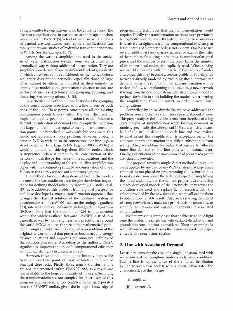
This expression can be easily calculated using for exam-ple a worksheet as in Figure 6
In this figure we consider a demand distributionat the (inner) points given by the values of 120582 (0246
0338 0954) the demand values given by the values(0171 0084 0329) of 120583 representing demand fractionsat those points according to (22) In the worksheet we canalso read besides the specific variable values used for thecalculations the value of 119865
119876= 08 used meaning that a
demand of 119876119889
= 08 sdot 119876in = 08 sdot 025 = 02m3s is ex-tracted in the line By using formula (24) implemented inthe cell below 119865
119876119889 we obtain the rate of demand that must be
allocated to the upstream end to get the correct piezometrichead at the downstream endThe graph in Figure 6 representsthis situation It can be clearly observed that the use of(24) provides a calculated HGL for the considered example(mid line) that perfectly matches the right end of the linerepresenting the real HGL (lower polygonal) On the otherhand the application of the 50 rule (upper HGL) producesunacceptable errors
24 Maximum Head Discrepancy When Using the Pro-posed Formula As mentioned before allocation of in-linedemands to the end nodes of a line may be of great interestin order to reduce the size of the mathematical model of aWDN In the previous section we have given formulae toobtain allocation values that zero the piezometric head errorat the downstream end of the line a mandatory conditionfor correct calculation on the line(s) connected to this endHowever this reduction of the model size is at the price ofmaking some piezometric head errors at the inner points ofthe line The engineer analyzing a WDN should be awareof the magnitude of those discrepancies in order to have abetter representation and understanding of the problem Inthis section we answer this question by solving problem (8)
8 Abstract and Applied Analysis
0000 100000 0000 100000 1000000246 95297 1000 93114 880250338 93979
08 02 0604 907630688 897750797 88705
0000 0000 0000 0954 880600246 0246 0171 0171 1000 880250338 0093 0084 02560604 0266 0017 02720688 0084 0078 03510797 0108 0321 06710954 0157 0329 10001000 0046
00000137 02460204 00690218 01680281 00520537 00560800 0034
00020626
026188000
90000
92000
94000
96000
98000
100000
0000 0200 0400 0600 0800 1000
H real
H real
HC (50)HC formula
H0 Qin L f D K 120582 120582 HC (50) HC formula
120582 120582k+1 minus 120582k 120583 Σ120583
FQ lowast Σ120583 (120582k+1 minus 120582k)(1 minus FQ lowast Σ120583)2
FQ Qd
025 500 0018 03 061205079100
FQ119889
Figure 6 Calculation of 119865119876119889
for a nonuniform distribution of demand within a line and comparison among hydraulic grade lines
In the (ideal) case of a continuous demand along the lineit is easy to show that (8) reduces to find the point 119909 wherethe derivatives with respect to 119909 of
119867119877(119865119876 119909) = 119867
0minus 119870int
119909
0
(119876in minus 119876 (119906))2d119906 (25)
119867119862(119865119876119889
119909) = 1198670minus 119870119909119876
2
in(1 minus 119865119876119889
119865119876)2 (26)
coincideLet us observe that 119867
119877(119865119876 119909) is a differentiable function
since 119876(119909) is continuous and that 119867119862(119865119876119889
119909) is a linearfunction of 119909 Thus it is easily seen that the maximumdiscrepancy is located at the point 119909 given by
119902 (119909) = 119865119876119889
(27)
Example 4 In the case of uniform continuous demand thesolution of (8) is given by
119909infin
= 119871119865infin
119876119889 (28)
obtained using 119902(119909) = 119909119871 as in Example 1 and (10)
In the (real) case of a discrete demand along the line themaximum discrepancy occurs at one of the points 119909
119896 since
the real HGL is a decreasing concave upwards polygonal (seeFigure 6) Then the problem reduces to identify the first 119909
1198960
for which the next section of the polygonal has a slope equalto or lower than the slope of119867
119862(119865119876119889
119909) in absolute values (ifequal all the points between 119909
1198960and 119909
1198960+1will provide the
maximum since the mentioned section of the polygonal and
119867119862(119865119876119889
119909)will run parallel between both points) So we haveto solve the following problem
Find the first point 1199091198960such that
119870(119876in minus (
1198960
sum
119894=1
119889119894))
2
le 1198701198762
in(1 minus 119865119876119889
119865119876)2
(29)
This inequality may be simplified and written in terms of120583119894 as
(1 minus 119865119876(
1198960
sum
119894=1
120583119894))
2
le (1 minus 119865119876119889
119865119876)2
(30)
which gives
1198960
sum
119894=1
120583119894ge 119865119876119889
(31)
in terms of 120583119894= 119889119894119876119889
That is to say the problem may be rewritten as follows
Find the first point 1199091198960
such that1198960
sum
119894=1
120583119894ge 119865119876119889
(32)
Example 5 In the case of uniform demand on 119899 equallyspaced points this gives the following
Find the first point1199091198960such that
1198960
sum
119894=1
1
119899=
1198960
119899=
119909119899
1198960
119871ge 119865119899
119876119889
(33)
Abstract and Applied Analysis 9
Observe that lim119899rarrinfin
(119909119899
1198960119871) ge lim
119899rarrinfin119865119899
119876119889= 119865infin
119876119889 since
119865119899
119876119889converges to 119865
infin
119876119889 We also have that lim
119899rarrinfin(119909119899
1198960minus1119871) le
lim119899rarrinfin
119865119899
119876119889= 119865infin
119876119889 But obviously these two limits are the
same As a result one has from (28) that
lim119899rarrinfin
119909119899
1198960
119871= 119865infin
119876119889=
119909infin
119871 (34)
Observe that 1199091198991198960
is the point where the polygonals (2)exhibit the biggest head discrepancy with the calculated headgiven by (9) corresponding to the allocation factor 119865119899
119876119889 Also
119909infin
is the point of maximum head discrepancy between theHGL corresponding to the uniform continuous demand andthe calculated head corresponding to the allocation factor119865infin
119876119889 As we could expect
lim119899rarrinfin
119909119899
1198960= 119909infin (35)
Expression (32) does not need any additional extra workin the general case if the calculations have been organizedas shown in Figure 6 In effect in this figure the first valueof the accumulated rated demand that exceeds 119865
119876119889= 0261
is sum1198960
119894=1120583119894
= 0272 which corresponds to the third innerdemand point 119909
1198960= 120582119871 with 120582 = 0604 This maximum is
119867119862(0261 119909
1198960) minus 119867119877(08 119909
1198960) = 92767 minus 90763 = 2003
(36)
3 Illustrative Example ona Real-World Network
This section is aimed to present some significant resultsobtained when applying the lessons learned in the previoussection to a practical situation The assessment is carried outin a real water supply network from Tegucigalpa City (thecapital of Honduras) The network which is intended to be adistrict metered area is supplied by onemain pipe connectedto one of the water tanks administered by the local waterauthority (SANAA)
The network has 203 nodes and 211 pipes Figure 7 showsthe network model in EPANET To illustrate the aspectspreviously studied three scenarios have been put forwardFor each scenario intermediate demand nodes (mid nodes)are placed in the main pipe In each case the demand valuesloaded in the intermediates nodes the distribution along theline or the pipe diameter vary as it is indicated as follows
Case A As it may be seen in Figure 8 an internal demandrepresenting 60 of the total inflow in the main line is fixedin two nodes placed along the line The first one loaded with25 of the total internal demand is located at 50 of the totallengthThe second intermediate node is located at 80 of thetotal length and the remaining 75 of the internal demand isallocated to it
Case B As shown in Figure 9 one single node is placed alongthe main line at 50 of its total length As it can be expected100 of the total internal demand is allocated to it In thiscase the internal demand represents 80 of the total inflow
Case C This case is fairly similar to Case B However in thiscase the diameter of the main line is reduced from 600mmto 450mm
31 Result (Case A) Figure 8 clearly reflects the character-istics and the results obtained for Case A First a hydraulicsimulation was conducted with the internal demand loadedin the mid nodes For that (real) case the pressure in nodeB (downstream node) is 4235 water column meters (wcm)When the internal demand is reallocated to the upstreamand downstream nodes following the 50 rule the resultvaries up to 122 wcm in comparison with the initial caseThrough the application of formula (24) a more suiteddemand allocation rule is found (2245 for the upstreamnode and 7755 for the downstream node) When this ruleis applied the resulting pressure value is as expected exactlythe same as in the (real) casewith the internal demand locatedin the mid nodes
32 Result (Case B and Case C) Given the fact that betweenCases B (Figure 9) and C (Figure 10) there is only onedifference namely the pipe diameter the allocation rulein both cases is the same 3486 of the internal demandshould be allocated to the upstream node and the rest tothe downstream node Nevertheless the differences betweenthe initial pressure values and the pressure obtained whenapplying the 50 allocation rule are larger in Case C than inCase B since in Case C the head loss is higher than that inCase B If Case A is included in the same comparison (higherhead loss than Cases B and C) the importance of a demandallocation based on the proposed methodology over a 50-50 becomes evident
Finally to better visualize the negative impact of using thecommon 50 demand distribution rule instead of the suitedrule (24) developed in this paper resulting pressure valuesobtained in four nodes of the example network (see Figure 11)are compared for Case A first when the demand is allocatedusing the 50 rule and then when the suited rule given byformula (24) is implementedThe results of such comparisonmay be seen in Table 2
4 Conclusions
The complexity of the interaction of all the input data ina mathematical model makes it impossible to include allthe data accurately The reality is very complex [2] and theuse of simplifications in order to make the model feasibleis therefore inevitable The use of such tools should bein any case accompanied by a clear understanding of theconsequences of such assumptions It is obvious that thelower level of simplification corresponds with more complextools In this sense software packages available in the marketdevoted to the analysis design and in general the simulationof the various states in a WDN should be used with thenecessary caution
This research focuses on the study of the influence thatthe concentration of a distributed demand in a line on theline ends represents in modeling steady state conditions in
10 Abstract and Applied Analysis
Table 2 Comparison among scenarios
Control pointScenario A1 Real
case (demand loadedin mid nodes)
Scenario A2Demand allocatedusing the suited rule
(24)
Scenario A3Demand allocatedusing the 50-50
rule
Differencesbetween A1 and
A2
Differencesbetween A1 and
A3
A 4135 4135 5356 0 1221B 2072 2072 3293 0 1221C 5339 5339 6560 0 1221D 327 3270 4491 0 1221
Line with internal demand
Figure 7 Water supply system used for the practical example
L = 500m
La = L lowast 05 Lb = L lowast 03 Lc = L lowast 02
Qin = 41704 lps
Head losses = 7068 mkm
QQQQnetwork = 16704 lps
Node Aallocateddemand
Q50 = 12500 lps(5000)
Qcal = 5614 lps(2245)
Pressurenode A(wcm)
7926
7926
7926
Mid node 1allocateddemand
Qmn1 = 625 lps(25)
Mid node 2allocateddemand
Qmn2 = 1875 lps(75)
Node Ballocateddemand
Q50 = 12500 lps(5000)
Qcal = 19386 lps(7755)
Pressurenode B
BA
(wcm)
4392
5613
4392
Figure 8 Details and results for Case A
Abstract and Applied Analysis 11
L = 600m
La = L lowast 05 Lb = L lowast 05
QQQin = 83505 lps
Head losses = 615 mkm
Qnetwork = 16704 lps
Node Aallocateddemand
Q50 = 33408 lps(5000)
Qcal = 23290 lps(3486)
Pressurenode A(wcm)
7926
7926
7926
Mid nodeallocateddemand
Qmn = 6682 lps(100)
Node Ballocateddemand
Q50 = 33408 lps(5000)
Qcal = 43526 lps(6514)
Pressurenode B(wcm)
7557
7671
7557
Figure 9 Details and results for Case B
L = 600m
La = L lowast 05 Lb = L lowast 05
Q QQin = 83505 lps
Head losses = 4363 mkm
Qnetwork = 16704 lps
Node Aallocateddemand
Q50 = 33408 lps(5000)
Qcal = 23290 lps(3486)
Pressurenode A(wcm)
7926
7926
7926
Mid nodeallocated
flow
Qmn = 6682 lps(100)
Node BNode Ballocated
demand
Q50 = 33408 lps(5000)
Qcal = 43526 lps(6514)
Pressure
BA
(wcm)
6370
6849
6370
Figure 10 Details and results for Case C
Control point A
Control point B
Control point C
Control point D
Figure 11 Pressure control points
12 Abstract and Applied Analysis
WDNsThe research work using a practical approach showsthe importance of the relation between the total inflow andthe flow that is extracted due to the load of demands in theline The distribution of the consumptions along the line alsogreatly influences the validity of the model After assessingthe error thatmay derive fromusing the generalized 50 rulewe obtain the general formula (24) that enables to allocate anarbitrary inner line demand to the line ends with zero errorat the downstream end of the line In addition we providea means to calculate the associated maximum head pointdiscrepancy
In Figure 6 we have shown that our proposal is straight-forward and involves direct methods that can be easilyapplied by any user of any WDN analysis package forexample using a very simple worksheet Existing networkmodels may be revised to replace if necessary the usedallocation values with he values provided by (24) whichproduce more reliable results For a new network modelusers may make an a priori decision on implementing theright simplifications so that a suitable tradeoff betweenmodelsimplification and accuracy is obtained
This study applies only to branched networks in whichthe flow direction is predefined The results do not strictlyapply to looped networks in which the definition of upstreamand downstream nodes cannot be known a priori and evenmay vary depending on the hourly demand in the networkand on the demand pattern used Nevertheless a numberof facts make the obtained results in this paper applicableto looped networks as well with a little extra work fromthe technician in charge of the analysis In effect firstly thelong lines susceptible of the considered simplification mustbe selected this task will not represent any problem for theexpert Secondly the expert will also be able to have a clearidea about the flow direction in most of those lines In caseof doubt he or she can use an initial analysis approach overspecific lines following the 50 rule and after the analysisgo back to the design to check the actual flow direction andmake a decision about the final direction of the flow and thevalues for 119865
119876119889 Perhaps a little more of iteration will enable
to get the final design Thirdly if the expert is not happywith the obtained results for one of the lines one has theopportunity to include in the model an additional point ofthe line where the maximum head discrepancy occurs at thepoint given by condition (32) This will divide the line intotwo new lines to which the same criteria may be appliedFourthly this solution of including an interior point of oneline into the model will be also useful in case if a line is fed byboth ends
In a future work wewill consider the inclusion of variablevalues for the factor 119865
119876119889in the demand curves assigned at the
ends of the challenging lines so that variations of the flowdirection in certain lines during the day may be consideredwhen running extended period simulations (EPSs)
Conflict of Interests
The authors declare that there is no conflict of interestsregarding the publication of this paper
Acknowledgments
This work has been funded as part of the Project IDAWASDPI2009-11591 by the Direccion General de Investigacion delMinisterio de Ciencia e Innovacion (Spain) with supplemen-tary support from ACOMP2011188 from the ConselleriadrsquoEducacio of the Generalitat Valenciana
References
[1] J Izquierdo R Perez and P L Iglesias ldquoMathematical modelsand methods in the water industryrdquo Mathematical and Com-puter Modelling vol 39 no 11-12 pp 1353ndash1374 2004
[2] J Izquierdo I Montalvo R Perez-Garcıa and A Matıas ldquoOnthe complexities of the design of water distribution networksrdquoMathematical Problems in Engineering vol 2012 Article ID947961 25 pages 2012
[3] D A Savic and J K Banyard Water Distribution Systems ICEPublishing London UK 2011
[4] I Montalvo Optimal design of water distribution systems byparticle swarm optimization [doctoral dissertation] UniversidadPolitecnica de Valencia Valencia Spain 2011
[5] EPA (Environmental Protection Agency) ldquoEPANETrdquo Decem-ber 2012 httpwwwepagovnrmrlwswrddwepanethtml
[6] B S Jung P F Boulos and D J Wood ldquoPitfalls of waterdistribution model skeletonization for surge analysisrdquo Journalof the AmericanWaterWorks Association vol 99 no 12 pp 87ndash98 2007
[7] J Izquierdo I Montalvo R Perez-Garcıa and F J IzquierdoldquoSon validas ciertas simplificaciones en el estudio de los tran-sitorios hidraulicosrdquo in X Seminario Iberoamericano de Planifi-cacion Proyecto y Operacion de Sistemas de Abastecimiento deAgua (SEREA rsquo11) Morelia Mexico 2011
[8] E J Anderson and K H Al-Jamal ldquoHydraulic-network simpli-ficationrdquo Journal of Water Resources Planning andManagementvol 121 no 3 pp 235ndash244 1995
[9] B Ulanicki A Zehnpfund and F Martınez ldquoSimplificationof water distribution network modelsrdquo in Proceedings of the2nd International Conference onHydroinformatics pp 493ndash500International Water Association Zurich Switzerland 1996
[10] W M Grayman and H Rhee ldquoAssessment of skeletonizationin network modelsrdquo in Proceedings of the Joint Conferenceon Water Resource Engineering and Water Resources Planningand Management R H Hotchkiss and M Glade Eds ASCEAugust 2000
[11] TMWalski D V Chase D A SavicWGrayman S Beckwithand E Koelle Advanced Water Distribution Modeling andManagement Haestad Methods Waterbury Conn USA 2003
[12] L Perelman and A Ostfeld ldquoWater distribution system aggre-gation for water quality analysisrdquo Journal of Water ResourcesPlanning and Management vol 134 no 3 pp 303ndash309 2008
[13] J W Deuerlein ldquoDecomposition model of a general watersupply network graphrdquo Journal of Hydraulic Engineering vol134 no 6 pp 822ndash832 2008
[14] WM Grayman RMurray andD A Savic ldquoEffects of redesignof water systems for security and water quality factorsrdquo inProceedings of the World Environmental and Water ResourcesCongress S Starrett Ed pp 1ndash11 ASCE May 2009
[15] L Perelman and A Ostfeld ldquoWater-distribution systems sim-plifications through clusteringrdquo Journal of Water ResourcesPlanning and Management vol 138 no 3 pp 218ndash229 2012
Abstract and Applied Analysis 13
[16] MHerrera J Izquierdo R Perez-Garcıa andDAyala-CabreraldquoWater supply clusters by multi-agent based approachrdquo inProceedings of the 12th Annual International Conference onWater Distribution Systems Analysis (WDSA rsquo10) pp 861ndash869ASCE September 2010
[17] M Herrera J Izquierdo R Perez-Garcıa and I MontalvoldquoMulti-agent adaptive boosting on semi-supervised water sup-ply clustersrdquo Advances in Engineering Software vol 50 pp 131ndash136 2012
[18] A Di Nardo and M Di Natale ldquoA heuristic design supportmethodology based on graph theory for district metering ofwater supply networksrdquo Engineering Optimization vol 43 no2 pp 193ndash211 2011
[19] O Giustolisi D Laucelli L Berardi and D A Savic ldquoCom-putationally efficient modeling method for large water networkanalysisrdquo Journal of Hydraulic Engineering vol 138 no 4 pp313ndash326 2012
[20] E Todini and S Pilati ldquoA gradient algorithm for the analysisof pipe networksrdquo in Computer Applications in Water Supply BCoulbeck and C H Orr Eds vol 1 pp 1ndash20 Research StudiesPress Taunton UK 1988
[21] W Rudin Principles of Mathematical Analysis InternationalSeries in Pure and Applied Mathematics McGraw-Hill NewYork NY USA 3rd edition 1976
[22] R G Bartle and D R Sherbert Introduction to Real AnalysisJohn Wiley amp Sons Ontario Canada 3rd edition 2000
Submit your manuscripts athttpwwwhindawicom
Hindawi Publishing Corporationhttpwwwhindawicom Volume 2014
MathematicsJournal of
Hindawi Publishing Corporationhttpwwwhindawicom Volume 2014
Mathematical Problems in Engineering
Hindawi Publishing Corporationhttpwwwhindawicom
Differential EquationsInternational Journal of
Volume 2014
Applied MathematicsJournal of
Hindawi Publishing Corporationhttpwwwhindawicom Volume 2014
Probability and StatisticsHindawi Publishing Corporationhttpwwwhindawicom Volume 2014
Journal of
Hindawi Publishing Corporationhttpwwwhindawicom Volume 2014
Mathematical PhysicsAdvances in
Complex AnalysisJournal of
Hindawi Publishing Corporationhttpwwwhindawicom Volume 2014
OptimizationJournal of
Hindawi Publishing Corporationhttpwwwhindawicom Volume 2014
CombinatoricsHindawi Publishing Corporationhttpwwwhindawicom Volume 2014
International Journal of
Hindawi Publishing Corporationhttpwwwhindawicom Volume 2014
Operations ResearchAdvances in
Journal of
Hindawi Publishing Corporationhttpwwwhindawicom Volume 2014
Function Spaces
Abstract and Applied AnalysisHindawi Publishing Corporationhttpwwwhindawicom Volume 2014
International Journal of Mathematics and Mathematical Sciences
Hindawi Publishing Corporationhttpwwwhindawicom Volume 2014
The Scientific World JournalHindawi Publishing Corporation httpwwwhindawicom Volume 2014
Hindawi Publishing Corporationhttpwwwhindawicom Volume 2014
Algebra
Discrete Dynamics in Nature and Society
Hindawi Publishing Corporationhttpwwwhindawicom Volume 2014
Hindawi Publishing Corporationhttpwwwhindawicom Volume 2014
Decision SciencesAdvances in
Discrete MathematicsJournal of
Hindawi Publishing Corporationhttpwwwhindawicom
Volume 2014 Hindawi Publishing Corporationhttpwwwhindawicom Volume 2014
Stochastic AnalysisInternational Journal of
2 Abstract and Applied Analysis
a single emitter leakage exponent for the entire network Thelast two simplifications in particular are inescapable whenworking with EPANET [5] a tool of water network analysisin general use worldwide Also some simplifications cantotally undermine studies of hydraulic transient phenomenain WDNs See for example [6 7]
Among the various simplifications used in the analy-sis of water distribution systems some are assumed in ageneralized way without additional introspection They aresimplifications derived from the different levels of granularityat which a network can be considered As mentioned beforereal water distribution networks especially those of largecities cannot be efficiently modeled in their entirety Inapproximate models some granulation reduction actions areperformed such as skeletonization grouping pruning andclustering See among others [8ndash18]
In particular one of these simplifications is the groupingof the consumptions associated with a line in one or bothends of the line These points concentrate all the existingconsumption points (users) within the line The need forimplementing this specific simplification is evident because afaithful consideration of demand would imply the inclusionof a large number of nodes equal to the number of consump-tion points In a branched network with few consumers thiswould not represent a major problem However problemsarise in WDNs with up to 30 connections per line (eg astreet pipeline) In a large WDN (eg a 500 kmWDN) itwould amount to considering about 150000 nodes whichis impractical when it comes to the construction of thenetwork model the performance of the calculations and thedisplay and understanding of the results This simplificationcopes with the continuity principle or conservation of massHowever the energy aspects are completely ignored
The methods for calculating demand load in the modelsare one of the least studied aspects despite the obvious impor-tance for defining model reliability Recently Giustolisi et al[19] have addressed this problem from a global perspectiveand have developed a matrix transformation approach thatchanges the classical solution of the nonlinear system ofequations describing aWDNbased on the conjugate gradient[20] into what they call enhanced global gradient algorithm(EGGA) Note that the solution in [20] is implementedwithin the widely available freeware EPANET 2 used in ageneralized way by many engineers and practitioners aroundthe world EGGA reduces the size of the mathematical prob-lem through a transformed topological representation of theoriginal network model that preserves both mass and energybalance equations and improves the numerical stability ofthe solution procedure According to the authors EGGAsignificantly improves the modelrsquos computational efficiencywithout sacrificing its hydraulic accuracy
However this solution although technically impeccablefrom a theoretical point of view exhibits a number ofpractical drawbacks Firstly those matrix transformationsare not implemented within EPANET and as a result arenot available to the huge community of its users Secondlythe transformations are too complex for most users of thisprogram and especially too complex to be incorporatedinto the EPANET toolkit given the in-depth knowledge of
programming techniques that their implementation wouldrequireThirdly the transformationmatricesmust previouslybe explicitly written even though obtaining these matricesis relatively straightforward the computational efficiency atleast in terms ofmemory needs is not evident One has to useseveral additional (very sparse) matrices of sizes or the orderof the number of resulting pipes times the number of originalpipes and the number of resulting pipes times the numberof unknown head nodes are explicitly used When solvingreal-world problems with hundreds of thousands of nodesand pipes this may become a serious problem Fourthly fornetworks already modeled by excluding those intermediatedemand nodes the solution of matrix transformation will beuseless Fifthly when planning and designing a new networkstarting from the household demand distribution it would beperhaps desirable to start building the model by performingthe simplification from the outset in order to avoid latercomplications
Compelled by those drawbacks we have addressed theproblem from another we claimmore practical point of viewThis paper analyzes the possible errors from the effect of usingcertain types of simplifications when loading demands inmodels specifically the widespread 50 rule which allocateshalf of the in-line demand to each line end We analyzeto what extent this simplification is acceptable or on thecontrary supply information that differs substantially fromreality Also we obtain formulae that enable to allocateinner line demand to the line ends with minimal errorFinally a calculation of themaximumhead point discrepancyassociated is provided
Our proposal involves simple direct methods that can beeasily applied by any user of anyWDNanalysis package sinceemphasis is not placed on programming ability but on howto make a decision about the technical aspect of simplifyingthemodel and thus load the demand properly Users havingalready developed models of their networks may revise theallocation rule used and replace it if necessary with thevalues provided by the new formulae what will enable themto obtain more reliable results Also users starting the modelof a new networkmaymake an a priori decision about how tosimplify the network and suitably implement the associatedsimplifications
We first present a simple case that enables us to shed lightonto the problem a single line with variable distribution andgranulation consumption is consideredThen an example of areal network is analyzed using the lessons learnedThe papercloses with a conclusions section
2 Line with Associated Demand
Let us first consider the case of a single line associated withsome internal consumption under steady state conditionSuch a line is representative of the simplest installation(a line between two nodes) with a given inflow rate Thecharacteristics of the line are
(i) length 119871
(ii) diameter119863
Abstract and Applied Analysis 3
(iii) upstream head (boundary condition at the upstreamnode)119867
0
(iv) friction factor 119891 with its associated line resistance119870 = 8119891(119892120587
21198635)
(v) inflow 119876inVarious demand scenarios of consumption in the line
may be tested Such scenarios are associated with two char-acteristics
(i) total demand in the line with regard to inflow(ii) specific distribution of the demand along the lineLet us assume that the flow consumed within the line
(total in-line demand) represents a percentage of the lineinflow If this fraction is represented by 119865
119876 0 lt 119865
119876le 1 the
actual demand in the line is given by the expression
119876119889= 119865119876119876in (1)
21 Uniformly Distributed Demand along the Line To startwith the study we will assume that the actual demand ofthe line is uniformly distributed into a number 119899 of equallyspaced interior points (nodes) 119899 can take a value rangingfrom 1 (in the case of a line with a single demand node in themiddle) to a large integer number (in the case of an equallydistributed demand throughout the line) Observe that wedo not consider any demand at the end nodes since we areonly interested in the line demand associatedwith the interiornodes
Figure 1 shows various distributions of piezometric headcorresponding to values of119865
119876equal to 1 08 06 and 04 for a
set of values of 1198711198631198670119891 and119876in To build Figure 1 we have
used the specific values 119871 = 500m119863 = 300mm1198670= 50m
119891 = 0018 and 119876in = 025m3s As mentioned before thedemand has been equally distributed among 119899 equally spacedinterior nodes Specifically in Figure 1 119899 takes the values1 3 7 11 19 and ldquoinfinityrdquo The ldquoinfinityrdquo case represents auniform continuous demand The various curves in Figure 1have straightforward interpretation
For the polygonal hydraulic grade lines (HGLs) made outof segments between consumption points the calculationscorrespond to the usual hydraulic calculation of losses Thepolygonals start at the boundary condition (0119867
0) the other
vertices being the 119899 + 1 points as follows
(119895119871
119899 + 11198670minus 119870
119871
119899 + 11198762
in
119895
sum
119896=1
(1 minus119896 minus 1
119899119865119876)
2
)
119895 = 1 119899 + 1
(2)
Let us call 119867119877(119865119876 119899 119909) these HGLs the subindex ldquo119877rdquo
standing for ldquorealrdquo distribution of piezometric head along theline as real demands are used to calculate (2)
The calculation for the ideal HGL corresponding to auniform continuous demand which is used here as the limitfor 119899 rarr infin of the discrete uniform distribution of demandsis performed by integrating the differential loss
Δ119867 = minus119870(119876in minus119876119889
119871119909)
2
Δ119909 (3)
along the line The value 119876119889119871 is the (constant) demand
per unit length and 119909 is the distance to the upstreamnode By integrating and using (1) the piezometric headcorresponding to this continuous loss is given by
119867119877(119865119876 119909) = 119867
0minus 119870
119871
3
1198762
in119865119876
[1 minus (1 minus 119865119876
119909
119871)
3
] (4)
which corresponds to the upper curve a cubic in each of thegraphs in Figure 1
It becomes clear that the greatest discrepancies occur forvalues of 119865
119876close to 1 (eg when a high percentage of the
inflow is consumed along the line)As mentioned before these ldquorealrdquo HGLs in Figure 1 have
been calculated according to the demand distribution atthe various inner points in the line However models oflarge WDNs do not usually take intermediate demands intoaccount in contrast the demand of each line is allocated tothe end nodes of the line the 50 rule being generally used
22 Allocation of In-Line Demand to the Line Ends Is the 50Rule Adequate Let 119865
119876119889be the factor that allocates a part of
the line distributed demand 119876119889 to its upstream end Thus
the demand assigned to this upstream node is 1198760= 119865119876119889
119876119889
As a result 119876119897= 119876in minus 119876
0is the flowrate through the line
Note that using (1)
119876119897= 119876in (1 minus 119865
119876119865119876119889
) (5)
Then the calculated head value 119867119862for a given value of
119865119876119889
is
119867119862(119865119876119889
119909) = 1198670minus 119870119876
2
119897119909 (6)
The HGL obtained is thus a straight line that connectsthe point (0119867
0)with the point (119871119867
119862(119865119876119889
119871))This last valuecorresponds to the calculated head at 119871 the downstreamnode
In Figure 2 dashed lines have been added to the firsttwo charts of Figure 1 These new HGLs have been calculatedto give the same piezometric head at the downstream nodeas the line corresponding to a demand concentrated in themiddle point 119899 = 1 for the case 119865
119876= 1 (left chart) and as
the line corresponding to a continuous demand for 119865119876= 08
(right chart) These lines have been obtained by allocating afraction of the interior line demand to the upstream nodeand the rest to the downstream node Analogous dashedlines can be obtained for other combinations of 119865
119876and
119899 If the allocated fractions to the line ends are differentthe corresponding (straight) lines (the lines given by thenumerical model with lumped demands at the ends of theline) will also be different
Two problems arise at this point
(a) Firstly it would be desirable to know the best alloca-tion of the total in-line demand to the line ends that isto say to know the value 119865
119876119889that solves the following
problem
Minimize119865119876119889
10038171003817100381710038171003817119867119862(119865119876119889
119909) minus 119867119877(119865119876lowast 119909)
10038171003817100381710038171003817 (7)
4 Abstract and Applied Analysis
FQ = 1 FQ = 08 FQ = 06 FQ = 04
50
48
46
44
42
40
38
36
34
50
48
46
44
42
40
38
36
34
50
48
46
44
42
40
38
36
34
50
48
46
44
42
40
38
36
340 250 500 0 250 500 0 250 500 0 250 500
Inf1911
731
Inf1911
731
Inf1911
731
Inf1911
731
Figure 1 Hydraulic grade lines in one single line for various uniform distributions of demand
FQ = 1 FQ = 0850
49
48
47
46
45
44
43
42
41
40
50
49
48
47
46
45
44
43
42
41
400 100 200 300 400 500 0 100 200 300 400 500
LumpInf1911
731
LumpInf1911
731
Figure 2 Examples of discrepancy between distributed and lumped demand models
for certain functional norm sdot where119867119862(119865119876119889
119909) iscalculated by (6) according to the lumped demandallocation to both line ends and119867
119877(119865119876lowast 119909) accounts
for the real demand distribution either calculatedby (2) or (4) (or any other more general expressioncorresponding to not uniformly distributed demand
which we address later) The asterisk denotes otherparameters such as 119899 in (2) which may appear in theexpression of119867
119877
(b) Secondly after having made a suitable line-end allo-cation decision it is of interest to know the actualdistribution of piezometric head errors on the line
Abstract and Applied Analysis 5
Table 1 Values of 119865119876119889
as a function of 119865119876and 119899 when solving (9)
119899 (order) 119865119876
02 04 06 08 101 (1) 0472 0438 0397 0349 02933 (2) 0485 0466 0442 0413 03767 (3) 0488 0473 0455 0432 040211 (4) 0489 0475 0457 0435 040719 (5) 0490 0477 0461 0441 0415inf (6) 0491 0479 0465 0446 0423
and specifically to identify at what point or points themaximum head discrepancy occurs
Maximize119909
10038171003817100381710038171003817119867119862(119865119876119889
119909) minus 119867119877(119865119876lowast 119909)
10038171003817100381710038171003817 (8)
We start by discussing (7) and then address (8) inSection 24
The solution of (7) is here constrained by the natureof the problem we have to adhere to the fact that one ormore lines (pipes) may be connected to the downstreamend of the considered line The connected lines need thecorrect piezometric head at 119871mdashupstream end for themmdashto suitably perform their respective calculations It meansthat the piezometric head at 119871 given by 119867
119862and 119867
119877 must
coincide That is to say (7) reduces in our case to
Solve 119867119862(119865119876119889
119871) = 119867119877(119865119876lowast 119871) for 119865
119876119889 (9)
By solving (9) the following expressions for 119865119876119889
areobtained
(i) Case of continuous demand
119865infin
119876119889(119865119876) =
1
119865119876
(1 minus radic1 minus (1 minus 119865
119876)3
3119865119876
) (10)
(ii) Case of demand equally distributed among 119899 equallydistributed nodes
119865(119899)
119876119889(119865119876) =
1
119865119876
(1 minus radic1
119899 + 1
119899+1
sum
119896=1
(1 minus119896 minus 1
119899119865119876)
2
) (11)
In Table 1 and in two-dimensional Figure 3 values for (10)and (11) for 119865
119876values between 02 and 1 and for 119899 varying
along the previously used values namely 1 3 7 11 19 andinfinity are presented Note that values 1 to 6 on the frontalaxis of Figure 3 symbolize as shown in Table 1 the values 119899 =
1 3 7 11 19 and infinity respectivelyThe following facts are remarkable
(i) These values are independent of the problem datanamely119867
0 119876in 119871 119863 and 119891 and depend only on 119865
119876
and 119899 in the case of (11) that is to say they dependon the magnitude and the pattern of the distributeddemand This is a very remarkable result since thepresent study thus becomes nondimensional and asa result completely general
0204
0608
1
03
035
04
045
05
123456
045ndash0504ndash045
035ndash0403ndash035
0406
Figure 3 Solution of (9) for 119865119876119889
(ii) The values of 119865119876119889
range from approximately 03 to05 This means that about 30ndash50 of the totaldemand must be allocated to the upstream node andthe remainder to the downstream node
(iii) The lowest 119865119876119889
values correspond to the most awk-ward cases the rate of demand is close to or equalsthe total inflow in the line and the demand is highlyconcentrated at a few points (upper right corner of thetable right front of the figure)
(iv) The highest 119865119876119889
values closer to 50 correspondto the less problematic cases meaning little totaldistributed demand in relation to the total inflow inthe line and widely distributed demand (lower leftcorner of the table bottom left of the figure) Thisvalue approaches 50 as the rate of inflow consumedin the line approaches zero (Observe that for both(10) and (11) lim
119865119876rarr0119865(sdot)
119876119889(119865119876) = 05)
(v) It is also worth noting that lim119899rarrinfin
119865119899
119876119889= 119865infin
119876119889for all
119865119876 that is to say the monotonic sequence of contin-
uous functions 119865119899119876119889
infin
119899=1converges to the continuous
function 119865infin
119876119889uniformly in [0 1] (Dini theorem see
eg [21 22]) This has a direct interpretation asthe continuous demand is the limit of a uniformlydistributed demand among an increasing number ofequally distributed points on the pipe
Asmentioned before it is commonpractice inmathemat-ical modeling of WSN engineering to distribute the line flowinto two parts 50 for the upstream node and 50 for thedownstream node which approximately coincides with whatis observed in Table 1 and Figure 3 except for cases wherethe demand line is highly concentrated and represents a largepercentage of the total flow through the line
As a result of what has been presented so far it can be saidthat for uniformly distributed in-line demand the usual 50rule seems in principle an appropriate solution provided
6 Abstract and Applied Analysis
that the inner demand of the line is small compared withthe pipe inflow and that such a demand is widely distributedHowever equal demand allocation to the end nodes of theline may produce important discrepancies since the studyhighlights the need for other assignments in certain cases
23 Arbitrary Demand along the Line To state the problemin its more general form let us now consider a demanddistribution on the line whose accumulated demand is givenby a function 119876(119909) = 119876
119889119902(119909) where 119902(119909) is the accumulated
demand ratio a function increasing monotonically from 0to 1 While 119867
119862is calculated as in (6) 119867
119877is calculated by
integrating the loss Δ119867 = minus119870(119876in minus 119876(119909))2Δ119909 through the
line [0 119871] as follows
119867119877(119865119876 119902 (119909) 119909) = 119867
0minus 119870int
119909
0
(119876in minus 119876 (119906))2d119906 (12)
Observe that this function is monotonically decreasingand concave upwards
Example 1 119902(119909) = 119909119871 for the case of continuous uniformdemand which by using (1) gives (4)
Using (12) and the expression (6) for 119867119862in 119871 written
using (5) as
119867119862(119865119876119889
119871) = 1198670minus 119870119871119876
2
in(1 minus 119865119876119889
119865119876)2
(13)
the equation119867119862= 119867119877in 119871may be rewritten as
minus1198701198711198762
in(1 minus 119865119876119889
119865119876)2
= minus119870int
119871
0
(119876in minus 119876 (119909))2d119909 (14)
By substituting
119876 (119909) = 119876in119865119876119902 (119909) (15)
one gets
119871(1 minus 119865119876119889
119865119876)2
= int
119871
0
(1 minus 119865119876119902 (119909))
2d119909 (16)
from where the following expression is readily obtained
119865119876119889
(119865119876) =
1
119865119876
(1 minus radic1
119871int
119871
0
(1 minus 119865119876119902 (119909))
2d119909) (17)
The general solution for the problem at hand when anarbitrary demand through the line is considered may onlybe solved after having a specific expression for 119902(119909) As aconsequence for arbitrary demands we will restrict ourselvesto the case of discrete demands on a finite number of pointsof the pipe as happens in real life
Example 2 Let us start by considering a single demandwithdrawn at a specific point of the line That is to say let usconsider a demand distribution given by
119902 (119909) = 120575 (119909 minus 1199091) (18)
109080706050403020100 02 04 06 08 1
FQ = 02
FQ = 04
FQ = 06
FQ = 08
FQ = 1
Figure 4 Demand allocation fraction to the upstream nodedepending on the location of a single withdrawal in the line
which concentrates the whole demand119876119889at 1199091 where 120575(sdot) is
the well-known Dirac deltaIn this case (12) is written as
119867119877(119865119876 120575 (119909 minus 119909
1) 119871)
= 1198670minus 119870int
119871
0
[119876in minus 119876119889120575 (119906 minus 119906
1)]2d119906
= 1198670minus 119870int
1199091
0
1198762
ind119906 minus 119870int
119871
1199091
(119876in minus 119876119889)2d119906
= 1198670minus 11987011990911198762
in minus 119870 (119871 minus 1199091) (119876in minus 119876
119889)2
= 1198670minus 119870119871119876
2
in (120582 + (1 minus 120582) (1 minus 119865119876)2)
(19)
where 120582 = 1199091119871 is the fraction of the pipe where the
concentrated demand is located from the originEquating again119867
119862= 119867119877at 119871 gives
119865119876119889
(119865119876 120582) =
1
119865119876
(1 minus radic120582 + (1 minus 120582) (1 minus 119865119876)2) (20)
As could be expected these values not only depend on119865119876
as in the case of uniform demand but also strongly dependon 120582 In Figure 4 we have plotted these values as a functionof 120582 for various instances of 119865
119876 namely 10 08 06 04 and
02As expected the worst cases occur once more for with-
drawals representing a large percentage of the inflow to theline For small in-line demands (see eg the curve for 119865
119876=
02 also calculate the limit of (20) for 119865119876approaching to
0) the demand should be allocated to the end nodes almostlinearly proportional to the relative distance of the demandpoint to the downstream end as is completely natural Incontrast this rule does not apply to large in-line demandsas their corresponding curves show by becoming less andless linear As an extreme case let us consider the case of119865119876
= 1 Various HGLs have been plotted in Figure 5 by
Abstract and Applied Analysis 7
100
98
96
94
92
90
88
86
84
82
800 100 200 300 400 500
5001025
0509
Figure 5 HGLs depending on the location of a single withdrawal inthe line and HGL (dashed line) corresponding to the 50 allocationrule
varying the location of the withdrawal point specifically forvalues 120582 = 01 025 05 and 09 The (straight dashed)line corresponding to the 50 allocation rule has alsobeen represented We can observe that only for 120582 = 025
does the dashed line match the correct piezometric headat the downstream end (also observe that the lower curvein Figure 4 corresponding to 119865
119876= 1 contains the point
(120582 119865119876119889
) = (025 05)) In the other cases disagreements arenot only important at the downstream end but all along theline
In the general case we consider 119902(119909) = sum119899
119896=1119889119896120575(119909 minus 119909
119896)
where 119889119896are the demands at points 119909
119896 with 0 lt 119909
1lt 1199092lt
sdot sdot sdot lt 119909119899minus1
lt 119909119899lt 119871 such that sum119899
119896=1119889119896= 119876119889
Example 3 119902(119909) = (1119899)sum119899
119896=1120575(119909 minus (119896(119899 + 1))119871) in the case
of uniformdemand at 119899 equally distributed points in the pipeThis demand produces the expression in (2)
In the general case119867119877is calculated by
119867119877(119865119876 119871)
= 1198670minus 11987011990911198762
in minus 119870 (1199092minus 1199091) (119876in minus 119889
1)2
minus 119870 (1199093minus 1199092) (119876in minus (119889
1+ 1198892))2
minus sdot sdot sdot minus 119870 (119909119899minus 119909119899minus1
)(119876in minus
119899minus1
sum
119896=1
119889119896)
2
minus 119870 (119871 minus 119909119899)(119876in minus
119899
sum
119896=1
119889119896)
2
(21)
By denoting
120583119894=
119889119894
119876119889
1205830= 0 120582
119894=
119909119894
119871 1205820= 0
120582119899+1
= 1 for 119894 = 1 119899
(22)
this expression can be written as
119867119877(119865119876 119871) = 119867
0minus 119870119871119876
2
in
119899
sum
119896=0
(120582119896+1
minus 120582119896)(1 minus 119865
119876
119896
sum
119895=0
120583119895)
2
(23)
Then equating again119867119862= 119867119877at 119871 gives
119865119876119889
(119865119876 120582 120583)
=1
119865119876
(1 minus radic
119899
sum
119896=0
(120582119896+1
minus 120582119896)(1 minus 119865
119876
119896
sum
119895=0
120583119895)
2
)
(24)
This expression can be easily calculated using for exam-ple a worksheet as in Figure 6
In this figure we consider a demand distributionat the (inner) points given by the values of 120582 (0246
0338 0954) the demand values given by the values(0171 0084 0329) of 120583 representing demand fractionsat those points according to (22) In the worksheet we canalso read besides the specific variable values used for thecalculations the value of 119865
119876= 08 used meaning that a
demand of 119876119889
= 08 sdot 119876in = 08 sdot 025 = 02m3s is ex-tracted in the line By using formula (24) implemented inthe cell below 119865
119876119889 we obtain the rate of demand that must be
allocated to the upstream end to get the correct piezometrichead at the downstream endThe graph in Figure 6 representsthis situation It can be clearly observed that the use of(24) provides a calculated HGL for the considered example(mid line) that perfectly matches the right end of the linerepresenting the real HGL (lower polygonal) On the otherhand the application of the 50 rule (upper HGL) producesunacceptable errors
24 Maximum Head Discrepancy When Using the Pro-posed Formula As mentioned before allocation of in-linedemands to the end nodes of a line may be of great interestin order to reduce the size of the mathematical model of aWDN In the previous section we have given formulae toobtain allocation values that zero the piezometric head errorat the downstream end of the line a mandatory conditionfor correct calculation on the line(s) connected to this endHowever this reduction of the model size is at the price ofmaking some piezometric head errors at the inner points ofthe line The engineer analyzing a WDN should be awareof the magnitude of those discrepancies in order to have abetter representation and understanding of the problem Inthis section we answer this question by solving problem (8)
8 Abstract and Applied Analysis
0000 100000 0000 100000 1000000246 95297 1000 93114 880250338 93979
08 02 0604 907630688 897750797 88705
0000 0000 0000 0954 880600246 0246 0171 0171 1000 880250338 0093 0084 02560604 0266 0017 02720688 0084 0078 03510797 0108 0321 06710954 0157 0329 10001000 0046
00000137 02460204 00690218 01680281 00520537 00560800 0034
00020626
026188000
90000
92000
94000
96000
98000
100000
0000 0200 0400 0600 0800 1000
H real
H real
HC (50)HC formula
H0 Qin L f D K 120582 120582 HC (50) HC formula
120582 120582k+1 minus 120582k 120583 Σ120583
FQ lowast Σ120583 (120582k+1 minus 120582k)(1 minus FQ lowast Σ120583)2
FQ Qd
025 500 0018 03 061205079100
FQ119889
Figure 6 Calculation of 119865119876119889
for a nonuniform distribution of demand within a line and comparison among hydraulic grade lines
In the (ideal) case of a continuous demand along the lineit is easy to show that (8) reduces to find the point 119909 wherethe derivatives with respect to 119909 of
119867119877(119865119876 119909) = 119867
0minus 119870int
119909
0
(119876in minus 119876 (119906))2d119906 (25)
119867119862(119865119876119889
119909) = 1198670minus 119870119909119876
2
in(1 minus 119865119876119889
119865119876)2 (26)
coincideLet us observe that 119867
119877(119865119876 119909) is a differentiable function
since 119876(119909) is continuous and that 119867119862(119865119876119889
119909) is a linearfunction of 119909 Thus it is easily seen that the maximumdiscrepancy is located at the point 119909 given by
119902 (119909) = 119865119876119889
(27)
Example 4 In the case of uniform continuous demand thesolution of (8) is given by
119909infin
= 119871119865infin
119876119889 (28)
obtained using 119902(119909) = 119909119871 as in Example 1 and (10)
In the (real) case of a discrete demand along the line themaximum discrepancy occurs at one of the points 119909
119896 since
the real HGL is a decreasing concave upwards polygonal (seeFigure 6) Then the problem reduces to identify the first 119909
1198960
for which the next section of the polygonal has a slope equalto or lower than the slope of119867
119862(119865119876119889
119909) in absolute values (ifequal all the points between 119909
1198960and 119909
1198960+1will provide the
maximum since the mentioned section of the polygonal and
119867119862(119865119876119889
119909)will run parallel between both points) So we haveto solve the following problem
Find the first point 1199091198960such that
119870(119876in minus (
1198960
sum
119894=1
119889119894))
2
le 1198701198762
in(1 minus 119865119876119889
119865119876)2
(29)
This inequality may be simplified and written in terms of120583119894 as
(1 minus 119865119876(
1198960
sum
119894=1
120583119894))
2
le (1 minus 119865119876119889
119865119876)2
(30)
which gives
1198960
sum
119894=1
120583119894ge 119865119876119889
(31)
in terms of 120583119894= 119889119894119876119889
That is to say the problem may be rewritten as follows
Find the first point 1199091198960
such that1198960
sum
119894=1
120583119894ge 119865119876119889
(32)
Example 5 In the case of uniform demand on 119899 equallyspaced points this gives the following
Find the first point1199091198960such that
1198960
sum
119894=1
1
119899=
1198960
119899=
119909119899
1198960
119871ge 119865119899
119876119889
(33)
Abstract and Applied Analysis 9
Observe that lim119899rarrinfin
(119909119899
1198960119871) ge lim
119899rarrinfin119865119899
119876119889= 119865infin
119876119889 since
119865119899
119876119889converges to 119865
infin
119876119889 We also have that lim
119899rarrinfin(119909119899
1198960minus1119871) le
lim119899rarrinfin
119865119899
119876119889= 119865infin
119876119889 But obviously these two limits are the
same As a result one has from (28) that
lim119899rarrinfin
119909119899
1198960
119871= 119865infin
119876119889=
119909infin
119871 (34)
Observe that 1199091198991198960
is the point where the polygonals (2)exhibit the biggest head discrepancy with the calculated headgiven by (9) corresponding to the allocation factor 119865119899
119876119889 Also
119909infin
is the point of maximum head discrepancy between theHGL corresponding to the uniform continuous demand andthe calculated head corresponding to the allocation factor119865infin
119876119889 As we could expect
lim119899rarrinfin
119909119899
1198960= 119909infin (35)
Expression (32) does not need any additional extra workin the general case if the calculations have been organizedas shown in Figure 6 In effect in this figure the first valueof the accumulated rated demand that exceeds 119865
119876119889= 0261
is sum1198960
119894=1120583119894
= 0272 which corresponds to the third innerdemand point 119909
1198960= 120582119871 with 120582 = 0604 This maximum is
119867119862(0261 119909
1198960) minus 119867119877(08 119909
1198960) = 92767 minus 90763 = 2003
(36)
3 Illustrative Example ona Real-World Network
This section is aimed to present some significant resultsobtained when applying the lessons learned in the previoussection to a practical situation The assessment is carried outin a real water supply network from Tegucigalpa City (thecapital of Honduras) The network which is intended to be adistrict metered area is supplied by onemain pipe connectedto one of the water tanks administered by the local waterauthority (SANAA)
The network has 203 nodes and 211 pipes Figure 7 showsthe network model in EPANET To illustrate the aspectspreviously studied three scenarios have been put forwardFor each scenario intermediate demand nodes (mid nodes)are placed in the main pipe In each case the demand valuesloaded in the intermediates nodes the distribution along theline or the pipe diameter vary as it is indicated as follows
Case A As it may be seen in Figure 8 an internal demandrepresenting 60 of the total inflow in the main line is fixedin two nodes placed along the line The first one loaded with25 of the total internal demand is located at 50 of the totallengthThe second intermediate node is located at 80 of thetotal length and the remaining 75 of the internal demand isallocated to it
Case B As shown in Figure 9 one single node is placed alongthe main line at 50 of its total length As it can be expected100 of the total internal demand is allocated to it In thiscase the internal demand represents 80 of the total inflow
Case C This case is fairly similar to Case B However in thiscase the diameter of the main line is reduced from 600mmto 450mm
31 Result (Case A) Figure 8 clearly reflects the character-istics and the results obtained for Case A First a hydraulicsimulation was conducted with the internal demand loadedin the mid nodes For that (real) case the pressure in nodeB (downstream node) is 4235 water column meters (wcm)When the internal demand is reallocated to the upstreamand downstream nodes following the 50 rule the resultvaries up to 122 wcm in comparison with the initial caseThrough the application of formula (24) a more suiteddemand allocation rule is found (2245 for the upstreamnode and 7755 for the downstream node) When this ruleis applied the resulting pressure value is as expected exactlythe same as in the (real) casewith the internal demand locatedin the mid nodes
32 Result (Case B and Case C) Given the fact that betweenCases B (Figure 9) and C (Figure 10) there is only onedifference namely the pipe diameter the allocation rulein both cases is the same 3486 of the internal demandshould be allocated to the upstream node and the rest tothe downstream node Nevertheless the differences betweenthe initial pressure values and the pressure obtained whenapplying the 50 allocation rule are larger in Case C than inCase B since in Case C the head loss is higher than that inCase B If Case A is included in the same comparison (higherhead loss than Cases B and C) the importance of a demandallocation based on the proposed methodology over a 50-50 becomes evident
Finally to better visualize the negative impact of using thecommon 50 demand distribution rule instead of the suitedrule (24) developed in this paper resulting pressure valuesobtained in four nodes of the example network (see Figure 11)are compared for Case A first when the demand is allocatedusing the 50 rule and then when the suited rule given byformula (24) is implementedThe results of such comparisonmay be seen in Table 2
4 Conclusions
The complexity of the interaction of all the input data ina mathematical model makes it impossible to include allthe data accurately The reality is very complex [2] and theuse of simplifications in order to make the model feasibleis therefore inevitable The use of such tools should bein any case accompanied by a clear understanding of theconsequences of such assumptions It is obvious that thelower level of simplification corresponds with more complextools In this sense software packages available in the marketdevoted to the analysis design and in general the simulationof the various states in a WDN should be used with thenecessary caution
This research focuses on the study of the influence thatthe concentration of a distributed demand in a line on theline ends represents in modeling steady state conditions in
10 Abstract and Applied Analysis
Table 2 Comparison among scenarios
Control pointScenario A1 Real
case (demand loadedin mid nodes)
Scenario A2Demand allocatedusing the suited rule
(24)
Scenario A3Demand allocatedusing the 50-50
rule
Differencesbetween A1 and
A2
Differencesbetween A1 and
A3
A 4135 4135 5356 0 1221B 2072 2072 3293 0 1221C 5339 5339 6560 0 1221D 327 3270 4491 0 1221
Line with internal demand
Figure 7 Water supply system used for the practical example
L = 500m
La = L lowast 05 Lb = L lowast 03 Lc = L lowast 02
Qin = 41704 lps
Head losses = 7068 mkm
QQQQnetwork = 16704 lps
Node Aallocateddemand
Q50 = 12500 lps(5000)
Qcal = 5614 lps(2245)
Pressurenode A(wcm)
7926
7926
7926
Mid node 1allocateddemand
Qmn1 = 625 lps(25)
Mid node 2allocateddemand
Qmn2 = 1875 lps(75)
Node Ballocateddemand
Q50 = 12500 lps(5000)
Qcal = 19386 lps(7755)
Pressurenode B
BA
(wcm)
4392
5613
4392
Figure 8 Details and results for Case A
Abstract and Applied Analysis 11
L = 600m
La = L lowast 05 Lb = L lowast 05
QQQin = 83505 lps
Head losses = 615 mkm
Qnetwork = 16704 lps
Node Aallocateddemand
Q50 = 33408 lps(5000)
Qcal = 23290 lps(3486)
Pressurenode A(wcm)
7926
7926
7926
Mid nodeallocateddemand
Qmn = 6682 lps(100)
Node Ballocateddemand
Q50 = 33408 lps(5000)
Qcal = 43526 lps(6514)
Pressurenode B(wcm)
7557
7671
7557
Figure 9 Details and results for Case B
L = 600m
La = L lowast 05 Lb = L lowast 05
Q QQin = 83505 lps
Head losses = 4363 mkm
Qnetwork = 16704 lps
Node Aallocateddemand
Q50 = 33408 lps(5000)
Qcal = 23290 lps(3486)
Pressurenode A(wcm)
7926
7926
7926
Mid nodeallocated
flow
Qmn = 6682 lps(100)
Node BNode Ballocated
demand
Q50 = 33408 lps(5000)
Qcal = 43526 lps(6514)
Pressure
BA
(wcm)
6370
6849
6370
Figure 10 Details and results for Case C
Control point A
Control point B
Control point C
Control point D
Figure 11 Pressure control points
12 Abstract and Applied Analysis
WDNsThe research work using a practical approach showsthe importance of the relation between the total inflow andthe flow that is extracted due to the load of demands in theline The distribution of the consumptions along the line alsogreatly influences the validity of the model After assessingthe error thatmay derive fromusing the generalized 50 rulewe obtain the general formula (24) that enables to allocate anarbitrary inner line demand to the line ends with zero errorat the downstream end of the line In addition we providea means to calculate the associated maximum head pointdiscrepancy
In Figure 6 we have shown that our proposal is straight-forward and involves direct methods that can be easilyapplied by any user of any WDN analysis package forexample using a very simple worksheet Existing networkmodels may be revised to replace if necessary the usedallocation values with he values provided by (24) whichproduce more reliable results For a new network modelusers may make an a priori decision on implementing theright simplifications so that a suitable tradeoff betweenmodelsimplification and accuracy is obtained
This study applies only to branched networks in whichthe flow direction is predefined The results do not strictlyapply to looped networks in which the definition of upstreamand downstream nodes cannot be known a priori and evenmay vary depending on the hourly demand in the networkand on the demand pattern used Nevertheless a numberof facts make the obtained results in this paper applicableto looped networks as well with a little extra work fromthe technician in charge of the analysis In effect firstly thelong lines susceptible of the considered simplification mustbe selected this task will not represent any problem for theexpert Secondly the expert will also be able to have a clearidea about the flow direction in most of those lines In caseof doubt he or she can use an initial analysis approach overspecific lines following the 50 rule and after the analysisgo back to the design to check the actual flow direction andmake a decision about the final direction of the flow and thevalues for 119865
119876119889 Perhaps a little more of iteration will enable
to get the final design Thirdly if the expert is not happywith the obtained results for one of the lines one has theopportunity to include in the model an additional point ofthe line where the maximum head discrepancy occurs at thepoint given by condition (32) This will divide the line intotwo new lines to which the same criteria may be appliedFourthly this solution of including an interior point of oneline into the model will be also useful in case if a line is fed byboth ends
In a future work wewill consider the inclusion of variablevalues for the factor 119865
119876119889in the demand curves assigned at the
ends of the challenging lines so that variations of the flowdirection in certain lines during the day may be consideredwhen running extended period simulations (EPSs)
Conflict of Interests
The authors declare that there is no conflict of interestsregarding the publication of this paper
Acknowledgments
This work has been funded as part of the Project IDAWASDPI2009-11591 by the Direccion General de Investigacion delMinisterio de Ciencia e Innovacion (Spain) with supplemen-tary support from ACOMP2011188 from the ConselleriadrsquoEducacio of the Generalitat Valenciana
References
[1] J Izquierdo R Perez and P L Iglesias ldquoMathematical modelsand methods in the water industryrdquo Mathematical and Com-puter Modelling vol 39 no 11-12 pp 1353ndash1374 2004
[2] J Izquierdo I Montalvo R Perez-Garcıa and A Matıas ldquoOnthe complexities of the design of water distribution networksrdquoMathematical Problems in Engineering vol 2012 Article ID947961 25 pages 2012
[3] D A Savic and J K Banyard Water Distribution Systems ICEPublishing London UK 2011
[4] I Montalvo Optimal design of water distribution systems byparticle swarm optimization [doctoral dissertation] UniversidadPolitecnica de Valencia Valencia Spain 2011
[5] EPA (Environmental Protection Agency) ldquoEPANETrdquo Decem-ber 2012 httpwwwepagovnrmrlwswrddwepanethtml
[6] B S Jung P F Boulos and D J Wood ldquoPitfalls of waterdistribution model skeletonization for surge analysisrdquo Journalof the AmericanWaterWorks Association vol 99 no 12 pp 87ndash98 2007
[7] J Izquierdo I Montalvo R Perez-Garcıa and F J IzquierdoldquoSon validas ciertas simplificaciones en el estudio de los tran-sitorios hidraulicosrdquo in X Seminario Iberoamericano de Planifi-cacion Proyecto y Operacion de Sistemas de Abastecimiento deAgua (SEREA rsquo11) Morelia Mexico 2011
[8] E J Anderson and K H Al-Jamal ldquoHydraulic-network simpli-ficationrdquo Journal of Water Resources Planning andManagementvol 121 no 3 pp 235ndash244 1995
[9] B Ulanicki A Zehnpfund and F Martınez ldquoSimplificationof water distribution network modelsrdquo in Proceedings of the2nd International Conference onHydroinformatics pp 493ndash500International Water Association Zurich Switzerland 1996
[10] W M Grayman and H Rhee ldquoAssessment of skeletonizationin network modelsrdquo in Proceedings of the Joint Conferenceon Water Resource Engineering and Water Resources Planningand Management R H Hotchkiss and M Glade Eds ASCEAugust 2000
[11] TMWalski D V Chase D A SavicWGrayman S Beckwithand E Koelle Advanced Water Distribution Modeling andManagement Haestad Methods Waterbury Conn USA 2003
[12] L Perelman and A Ostfeld ldquoWater distribution system aggre-gation for water quality analysisrdquo Journal of Water ResourcesPlanning and Management vol 134 no 3 pp 303ndash309 2008
[13] J W Deuerlein ldquoDecomposition model of a general watersupply network graphrdquo Journal of Hydraulic Engineering vol134 no 6 pp 822ndash832 2008
[14] WM Grayman RMurray andD A Savic ldquoEffects of redesignof water systems for security and water quality factorsrdquo inProceedings of the World Environmental and Water ResourcesCongress S Starrett Ed pp 1ndash11 ASCE May 2009
[15] L Perelman and A Ostfeld ldquoWater-distribution systems sim-plifications through clusteringrdquo Journal of Water ResourcesPlanning and Management vol 138 no 3 pp 218ndash229 2012
Abstract and Applied Analysis 13
[16] MHerrera J Izquierdo R Perez-Garcıa andDAyala-CabreraldquoWater supply clusters by multi-agent based approachrdquo inProceedings of the 12th Annual International Conference onWater Distribution Systems Analysis (WDSA rsquo10) pp 861ndash869ASCE September 2010
[17] M Herrera J Izquierdo R Perez-Garcıa and I MontalvoldquoMulti-agent adaptive boosting on semi-supervised water sup-ply clustersrdquo Advances in Engineering Software vol 50 pp 131ndash136 2012
[18] A Di Nardo and M Di Natale ldquoA heuristic design supportmethodology based on graph theory for district metering ofwater supply networksrdquo Engineering Optimization vol 43 no2 pp 193ndash211 2011
[19] O Giustolisi D Laucelli L Berardi and D A Savic ldquoCom-putationally efficient modeling method for large water networkanalysisrdquo Journal of Hydraulic Engineering vol 138 no 4 pp313ndash326 2012
[20] E Todini and S Pilati ldquoA gradient algorithm for the analysisof pipe networksrdquo in Computer Applications in Water Supply BCoulbeck and C H Orr Eds vol 1 pp 1ndash20 Research StudiesPress Taunton UK 1988
[21] W Rudin Principles of Mathematical Analysis InternationalSeries in Pure and Applied Mathematics McGraw-Hill NewYork NY USA 3rd edition 1976
[22] R G Bartle and D R Sherbert Introduction to Real AnalysisJohn Wiley amp Sons Ontario Canada 3rd edition 2000
Submit your manuscripts athttpwwwhindawicom
Hindawi Publishing Corporationhttpwwwhindawicom Volume 2014
MathematicsJournal of
Hindawi Publishing Corporationhttpwwwhindawicom Volume 2014
Mathematical Problems in Engineering
Hindawi Publishing Corporationhttpwwwhindawicom
Differential EquationsInternational Journal of
Volume 2014
Applied MathematicsJournal of
Hindawi Publishing Corporationhttpwwwhindawicom Volume 2014
Probability and StatisticsHindawi Publishing Corporationhttpwwwhindawicom Volume 2014
Journal of
Hindawi Publishing Corporationhttpwwwhindawicom Volume 2014
Mathematical PhysicsAdvances in
Complex AnalysisJournal of
Hindawi Publishing Corporationhttpwwwhindawicom Volume 2014
OptimizationJournal of
Hindawi Publishing Corporationhttpwwwhindawicom Volume 2014
CombinatoricsHindawi Publishing Corporationhttpwwwhindawicom Volume 2014
International Journal of
Hindawi Publishing Corporationhttpwwwhindawicom Volume 2014
Operations ResearchAdvances in
Journal of
Hindawi Publishing Corporationhttpwwwhindawicom Volume 2014
Function Spaces
Abstract and Applied AnalysisHindawi Publishing Corporationhttpwwwhindawicom Volume 2014
International Journal of Mathematics and Mathematical Sciences
Hindawi Publishing Corporationhttpwwwhindawicom Volume 2014
The Scientific World JournalHindawi Publishing Corporation httpwwwhindawicom Volume 2014
Hindawi Publishing Corporationhttpwwwhindawicom Volume 2014
Algebra
Discrete Dynamics in Nature and Society
Hindawi Publishing Corporationhttpwwwhindawicom Volume 2014
Hindawi Publishing Corporationhttpwwwhindawicom Volume 2014
Decision SciencesAdvances in
Discrete MathematicsJournal of
Hindawi Publishing Corporationhttpwwwhindawicom
Volume 2014 Hindawi Publishing Corporationhttpwwwhindawicom Volume 2014
Stochastic AnalysisInternational Journal of
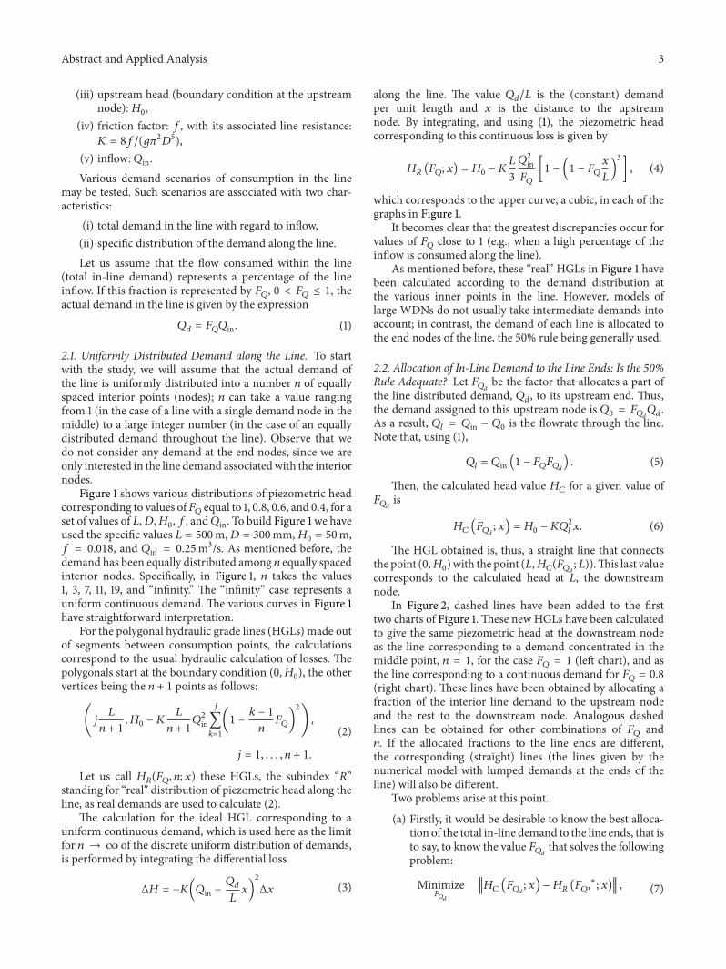
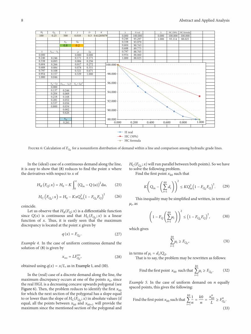