This is an almost final version of the paper ’J. Gasteiger, C. Emde, B. Mayer, R. Buras, S.A. Buehler, and O.Lemke. Representative wavelengths absorption parameterization applied to satellite channels and spectral bands. J.Quant. Spectrosc. Radiat. Transfer, 148, 99-115, 2014’.

All changes during the review process are considered, but minor changes performed after acceptance of the papermay be missing.

The final paper is provided at https://doi.org/10.1016/j.jqsrt.2014.06.024 or upon request to developers@libradtran.org

Representative wavelengths absorption parameterization applied to satellitechannels and spectral bands

J. Gasteigera,∗, C. Emdea, B. Mayera, R. Burasa, S. A. Buehlerb,c, O. Lemkeb,c

aMeteorologisches Institut, Ludwig-Maximilians-Universitat, Theresienstr. 37, Munchen, GermanybSRT, Luleå University of Technology, Rymdcampus 1, Kiruna, Sweden

cNow at: Meteorological Institute, University of Hamburg, Bundesstraße 55, Hamburg, Germany

Abstract

Accurate modeling of wavelength-integrated radiative quantities, e.g. integrated over a spectral band or an instrumentchannel response function, requires computations for a large number of wavelengths if the radiation is affected by gasabsorption which typically comprises a complex line structure. In order to increase computational speed of modelingradiation in the Earth’s atmosphere, we parameterized wavelength-integrals as weighted means over representativewavelengths. We parameterized spectral bands of different widths (1 cm−1, 5 cm−1, and 15 cm−1) in the solar andthermal spectral range, as well as a number of instrument channels on the ADEOS, ALOS, EarthCARE, Envisat,ERS, Landsat, MSG, PARASOL, Proba, Sentinel, Seosat, and SPOT satellites. A root mean square relative deviationlower than 1% from a ”training data set” was selected as the accuracy threshold for the parameterization of each bandand channel. The training data set included high spectral resolution calculations of radiances at the top of atmospherefor a set of highly variable atmospheric states including clouds and aerosols. The gas absorption was calculated fromthe HITRAN 2004 spectroscopic data set and state-of-the-art continuum models using the ARTS radiative transfermodel. Three representative wavelengths were required on average to fulfill the accuracy threshold. We implementedthe parameterized spectral bands and satellite channels in the uvspec radiative transfer model which is part of thelibRadtran software package. The parameterization data files, including the representative wavelengths and weightsas well as lookup tables of absorption cross sections of various gases, are provided at the libRadtran webpage.

In the paper we describe the parameterization approach and its application. We validate the approach by com-paring modeling results of parameterized bands and channels with results from high spectral resolution calculationsfor atmospheric states that were not part of the training data set. Irradiances are not only compared at the top ofatmosphere but also at the surface for which this parameterization approach was not optimized. It is found that theparameterized bands and channels provide a good compromise between computation time requirements and uncer-tainty for typical radiative transfer problems. In particular for satellite radiometer simulations the computation timerequirement and the parameterization uncertainty is low. Band-integrated irradiances at any level as well as heatingand cooling rates below 20 km can also be modeled with low uncertainty.

Keywords:Band parameterization, Satellite channel parameterization, Gas absorption, Radiative transfer, Earth’s atmosphere

∗Corresponding author. Phone: +49 89 2180 4386, Fax: +49 89 2180 4182, Email: josef.gasteiger@lmu.de.

Preprint submitted to Journal of Quantitative Spectroscopy and Radiative Transfer July 12, 2018

1. Introduction

Modeling of wavelength-integrated radiative quantities is required frequently in atmospheric science, e.g. forsimulating irradiances or radiances measured by remote sensing instruments. It requires the radiative transfer problemto be solved at a large number of wavelengths if the spectral range is affected by fine-structured absorption features ofgases, making it computationally expensive. Fine-structured gas absorption features exist in large parts of the visibleand infrared spectral range.

Different parameterization approaches are available for reducing the computational cost of such modeling prob-lems. The most prominent general approach is the k-distribution approach. The basic idea of the k-distribution ap-proach is to sort the wavelength grid such that the gas absorption coefficient on the reordered wavelength grid is smoothand monotonic; with the reordered grid, the spectral integration of radiative quantities requires much less wavelengthgrid points. The optimum ordering depends on pressure, temperature, and gas concentration. Many k-distributionmethods use the assumption that the gas absorption spectra of the different atmospheric layers are correlated withthe gas absorption spectrum of a reference layer [1]. Such correlated-k distribution methods are used for example byKato [2] and Fu [3] for wide spectral bands, and by Kratz [4] for AVHRR satellite channels. A k-distribution methodnot employing the correlation assumption is described for example by Doppler et al. [5] which builds upon the so-called Spectral Mapping Transformation using k-distributions whose validity was tested at all atmospheric layers.Another parameterization approach employing k-distribution methods is LOWTRAN where the transmittance of thegases within 20 cm−1 wide bands is approximated by the sum of up to three exponential terms [6]. LOWTRAN7 isimplemented in the uvspec radiative transfer model which is part of the freely available libRadtran toolbox [7] whereit has been used frequently for spectral calculations and simulations of satellite channel responses. The gas absorptionproperties of LOWTRAN are based on HITRAN. Recent comparisons of measured thermal downward irradiances inthe atmospheric window around 10 µm with LOWTRAN calculations have revealed some discrepancies, whereas highspectral resolution calculations using HITRAN 2004 [8] data show good agreement [9]. The commercially availableMODTRAN code [10] also includes significantly improved spectral band parameterizations.

Buehler et al. [11] describe an approach for parameterizing gas absorption, where spectrally-integrated radiancesare approximated by weighted means of radiances at so-called representative frequencies or wavelengths. The rep-resentative wavelengths together with their weights are selected by an optimization method which minimizes thedeviation from the accurate spectrally-integrated radiances for a set of highly variable atmospheric states. Buehler etal. [11] focus on clear sky cases and parameterize thermal radiation channels of the HIRS satellite instrument. Wedeveloped a parameterization approach which is based on this work but includes adjustments to improve its applica-bility. For example, we added aerosols, water clouds, and ice clouds in the set of atmospheric states and increasedthe variability of the gas profiles. Furthermore, our approach determines automatically the number of representativewavelengths required to fulfill a parameterization accuracy threshold. Using this approach, we parameterized a largeset of narrow spectral bands of different widths covering the thermal as well as the solar spectral range. Spectralresponse functions of many satellite channels were parameterized in addition (a list of channels is provided in Ap-pendix A). We implemented the parameterized bands and channels, referred to as “REPTRAN” in the following, inthe uvspec model [7]. The REPTRAN data files are available from the libRadtran webpage - http://libradtran.org.

In Section 2 we describe the representative wavelengths parameterization approach. After that, in Section 3, weapply the parameterization approach to spectral bands and satellite channels, investigate the spectral variability ofthe considered gas absorption, and compare results from parameterized bands and channels with results from exacthigh spectral resolution (HSR) calculations. We perform these comparisons for irradiances at the top of atmosphere,for which REPTRAN has been optimized, and also for irradiances at the surface and for heating rates as function ofheight. We also consider the LOWTRAN parameterization for the comparisons because it has been one of the mostlyused absorption parameterizations of the uvspec model.

2. Methodology

2.1. Parameterization approach for spectral integrals

We parameterized spectrally-integrated radiative quantities by weighted means of these quantities at representativewavelengths, following the approach described by Buehler and coauthors [11] for broadband infrared radiometers.

2

Table 1: Parameters of aerosol and cloud layers in training set of atmospheres.

parameter sampling aerosol water cloud ice cloudmodel Mie Mie Key/Yang [13]reff log 0.1 - 10 µm 1 - 15 µm habit-dependentmr lin 1.28 - 2.00 - -mi log 0.001 - 0.1 - -zbottom lin 0 - 15 km 0 - 8 km 4 - 15 km∆z 1 km 1 km 1 kmτ log 0.1 - 2 1 - 20 1 - 20# cases 420 168 168

The basic idea of the parameterization approach is given by

Iint =

∫ λmax

λmin

I(λ)R(λ)dλ ≈ Iint,para = Rint ·

nrep∑irep=1

I(λirep )wirep (1)

with Rint =

∫ λmax

λmin

R(λ)dλ

The spectrally-integrated radiative quantity Iint is the integral of the spectral radiative quantity I(λ) times the spectralweighting function R(λ) (with 0 ≤ R(λ) ≤ 1) from the limits λmin to λmax of the spectral interval. R(λ) can describe,for example, an instrument channel response function or a wavelength band. Iint is approximated by Iint,para, which isthe sum of the spectral radiative quantity I at nrep representative wavelengths λirep multiplied by their weights wirep andthe term Rint. The sum over the weights wirep is equal to 1, thus the summation term of Eq. 1 is a weighted mean of thequantity I. The term Rint is a measure for the spectral width of the interval.

For each spectral interval, the set of representative wavelengths λirep and weights wirep needs to be optimized. Ourmethodology is based on Buehler et al. [11] with some modifications as described below. The optimization approachuses spectrally high-resolved radiances of a set of different atmospheric states, the ’training set of atmospheres’.

2.1.1. Training set of atmospheresOur aim is developing a parameterization approach which approximates wavelengths integrals for any realistic

atmosphere of the Earth with low uncertainty. Thus, it is required that the variability present in the Earth’s atmosphereis covered by the atmospheric profiles of the training data set. As a starting point, we selected the data set of Garand etal. [12] as used by Buehler et al. [11]: This data set includes 42 profiles of temperature, pressure, and volume mixingratios of H2O, O3, CO2, N2O, CO, and CH4. For O2 and N2 we assumed height-constant volume mixing ratios of0.2095 and 0.7808, respectively. The top height of the profiles varies between 61 km and 67 km.

We investigated the variability of these 42 gas atmospheres and found that the variability of CO2, N2O, CO, andCH4 does not cover the variability present in the Earth’s atmosphere. Thus, we created for each of the 42 atmospheresa second gas atmosphere in which we halved the volume mixing ratios of one of CO2, N2O, CO, and CH4 and doubledthe volume mixing ratios of another one of these species, choosing the respective species randomly. Furthermore, theNO2 profile from the US standard atmosphere is added to all 84 gas atmospheres.

We added cloud and aerosol layers to these gas atmospheres: For each gas atmosphere, one clear sky case, 5aerosol cases, 2 water cloud cases, and 2 ice cloud cases are considered. Thus, the training data set consists of840 different atmospheres. The microphysical properties of the aerosol and cloud particles and the heights of thelayers were chosen randomly using either linear or logarithmic sampling according to the ranges given in Tab. 1. Weconsidered a wide range of effective radii reff , layer bottom heights zbottom, and optical thicknesses τ for both aerosolsand clouds. In case of aerosols we considered also a wide range of wavelength-independent refractive indices m =

mr + mii. We fixed the widths of the log-normal aerosol size distributions to σ = 2. The water cloud droplet sizedistribution are gamma distributions with an effective variance of veff = 0.1. For the ice clouds we considered the

3

Start nrep

=1 Ncomb

<107

systematicsearch

simulatedannealing

set ofλ

irep& w

irep

Δpara

<1% Stop

nrep

= nrep

+1

Δpara

<1.5%

& simulated annealingused once for

current nrep

yes

no

yes

noyes

no

Figure 1: Flow chart for selection of representative wavelengths for a given spectral interval.

habits ’solid-column’, ’hollow-column’, ’rough-aggregate’, ’rosette-6’, ’plate’, and ’droxtal’ [13]. All aerosol andcloud layers have a vertical extent of ∆z = 1 km.

2.1.2. High spectral resolution calculationsWe performed high spectral resolution calculations for these atmospheres in the wavelength range from λ ≈ 395

nm to λ = 100 µm using a constant spectral resolution of 119.917 monochromatic calculations per cm−1. This samplingrate corresponds to about ∆λ = 0.0002 nm at λ = 500 nm and ∆λ = 0.0834 nm at λ = 10 µm, and a total of about3 million wavelengths. The selected sampling rate is sufficient for the absorption in the lower atmosphere but maynot sample all absorption features present in the upper atmosphere, where absorption lines can be quite narrow dueto weak pressure broadening. However, such narrow absorption lines in the upper atmosphere typically are of littlerelevance for spectrally-integrated radiances or irradiances.

As the first step, the spectral absorption profiles of the 84 gas atmospheres (excluding the absorption data listed insubsequent paragraph) were calculated using the radiative transfer model ARTS [14]. The absorption was calculatedfrom line parameters of the HITRAN 2004 spectroscopic database [8] for the above-mentioned eight gas species.MT CKD (version 1.0) continuum absorption data [15] for H2O, CO2, N2, and the collision-induced absorption byO2 around λ = 6.4 µm was added to the absorption profiles. Hitherto the ARTS model has not been applied in thevisible spectral range.

Using the gas absorption profiles from ARTS, the DISORT radiative transfer solver [16], implemented in uvspec[7], was utilized to calculate the high spectral resolution radiances of the 840 atmospheres at their top. The calculationswere performed for solar radiation using the Kurucz solar spectrum [17], as well as for thermal radiation. Uvspecadds the following gas absorption data to the gas absorption profiles calculated by ARTS: (a) O3 absorption data fromMolina [18] for λ ≤ 850 nm, (b) collision-induced absorption by O2 from Greenblatt [19] for λ ≤ 1.13 µm, and (c)absorption by NO2 from Burrows [20] for λ ≤ 794 nm. For each atmospheric state, the surface albedo as well as fivecosines of viewing zenith angles were chosen randomly between 0 and 1. In case of solar radiation, two sun positionswere considered with the cosines of the solar zenith angles chosen randomly between 0 and 1 and the relative azimuthangles (between observer and sun) chosen randomly between 0◦ and 180◦. In total, Nrad = 8400 and Nrad = 4200spectral radiances have been calculated for solar and thermal radiation, respectively.

2.1.3. Optimization of representative wavelengthsThe representative wavelengths for each spectral interval are selected such that

∆para =

√√√1

Nrad

Nrad∑irad=1

(Iint,para,irad − Iint,irad

Iint,irad

)2

(2)

is below 1%. ∆para is the root mean square relative deviation of the parameterized radiances Iint,para w.r.t. the trainingdata set.

4

0 0.1 0.2 0.3 0.4 0.5 0.6 0.7 0.8 0.9

1

9100 9200 9300 9400 9500 9600 9700 9800 9900 10000

resp

onse

/ w

eig

ht

wavelength [nm]

channel responseoptimization for Δparaoptimization for Δ'para

Figure 2: Response function (red line) of Meteosat Second Generation infrared channel around λ = 9.7 µm; the blue boxes show representativewavelengths optimized for small ∆para, whereas the green circles show representative wavelengths optimized for small ∆′para; the weigth of eachrepresentative wavelength can be read from the vertical axis.

A flow chart of the selection procedure is shown in Fig. 1. The selection starts with the number of representativewavelengths nrep set to 1, and nrep is increased until ∆para has fallen below the 1% threshold. All nhsr wavelengths fromthe high spectral resolution calculations in the range λmin to λmax are candidates for representative wavelengths. Fora given number of representative wavelengths nrep, the representative wavelengths are optimized using two differentapproaches: If the number of possible wavelengths combinations Ncomb, which is given by

Ncomb =

(nhsrnrep

)(3)

is below 107, the optimum combination is searched systematically. If Ncomb is larger, the systematic search becomesimpractical and the wavelengths combination is optimized using simulated annealing as described by Buehler et al.[11]. Simulated annealing not necessarily finds the absolute optimum wavelengths combination for a given nrep;thus, a second simulated annealing run with the same nrep is performed if ∆para < 1.5% was achieved by simulatedannealing. We increase nrep by 1 in any other case if ∆para < 1% was not achieved.

When determining the representative wavelengths optimizing for small ∆para (Eq. 2) we found that often wave-lengths were selected where the spectral response function is small. An example is shown in Fig. 2 where the blueboxes illustrate the wavelengths λirep and their weights selected for a spectral response function R(λ) of a MSG2 in-frared channel (red line). Representative wavelengths with low R(λirep ) can reduce the robustness of the approach inparticular if an atmospheric constituent with a strong spectral variability that has not been considered in our trainingdata set is modeled. To punish the selection of such wavelengths we defined ∆′para which adds an extra factor to ∆para:

∆′para = ∆para ·

1 +

√√√1

nrep

nrep∑irep=1

( wirep

R(λirep )

)2 . (4)

Our approach optimizes the wavelengths combination for small ∆′para during the systematic search and during simu-lated annealing (Fig. 1). The effect of optimizing for small ∆′para instead of small ∆para is illustrated by Fig. 2: whencomparing the blue boxes with the green circles it becomes clear that optimizing for ∆′para (green circles) generatesrepresentative wavelengths only where R(λ) is not small. The weights wirep for a given wavelengths combination arealways determined using a nonnegative least squares routine that optimizes for small ∆para.

5

2.2. Parameterized spectral intervals

We applied this parameterization approach to narrow spectral bands and to spectral response functions of satelliteinstrument channels in the solar and thermal spectral range. To create the sets of spectral bands, we divided thewavelength spectrum into adjacent non-overlapping bands with three different widths: A coarse case with band widthsof 15 cm−1, a medium case with 5 cm−1, and a fine case with 1 cm−1. We consider solar radiation in the range fromλ ≈ 395 nm (25315 cm−1) to λ ≈ 5025 nm (1990 cm−1), which results in 1555, 4665, or 23325 bands, depending onthe band widths. For radiation from thermal emission, the range from λ = 2.5 µm (4000 cm−1) to λ = 100 µm (100cm−1) is covered by 260, 780, or 3900 bands, depending on the band widths. The spectral weight R(λ) of a band fromλmin to λmax is defined as R(λ) = 1 for λ ∈ [λmin, λmax]. In addition to these spectral bands, we have parameterizedspectral response functions of almost 400 channels of instruments on the ADEOS, ALOS, EarthCARE, Envisat, ERS,Landsat, MSG, PARASOL, Proba, Sentinel, Seosat, and SPOT satellites (a list of channels is provided in AppendixA). We have implemented the parameterized bands and satellite instrument channels in the uvspec radiative transfermodel.

2.3. Absorption lookup tables

The absorption cross sections Cabs of gas molecules at the representative wavelengths are required for the appli-cation of the parameterized spectral intervals in radiative transfer calculations. Following the approach of Buehler etal. [21], lookup tables of pre-calculated absorption cross sections are used to provide the required data to the uvspecmodel. The lookup tables contain absorption cross sections of H2O, O3, CO2, N2O, CO, CH4, O2, and N2 on a grid ofpressures p and temperatures T . The water vapour absorption also depends on the water vapour mixing ratio xH2O. Thecross sections were calculated using the ARTS model based on HITRAN 2004 line data [8] together with MT CKDabsorption continua [15] for H2O, CO2, N2, and O2 (same data as described in Sect. 2.1.2). The grid of p, T , andxH2O is modified compared with the ’wide’ setup described by [21]: the spacing of the p grid, in terms of log p, is lessdense at high altitudes than at low altitudes, which is justified by comparatively low gas abundances at high altitudes;we use 41 p grid points, from 110000 Pa to 0.0007 Pa with a step of 2−0.25 from 110000 Pa to 46249 Pa, then 2−0.5

till 90 Pa, and finally 1/2 for lower pressures. The temperature T at each pressure level p is perturbed relative to thetemperature of the US standard atmosphere [22] by 0 K, ±20 K, ±40 K, ±70 K, and ±120 K. For water vapour, crosssections are calculated for mixing ratios xH2O = 0, 0.02, 0.05, and 0.10.

We converted the lookup tables of absorption cross sections from ARTS to a format readable by uvspec. In orderto reduce the file sizes, the converted lookup tables consist of one file per species and consider only representativewavelengths where the species absorbs. For calculating the absorption cross sections of the gas molecules at the p,T , and xH2O of interest, uvspec applies linear interpolation between the grid points of the lookup tables. Alongsidewith the cross sections from the lookup tables, uvspec considers also the independent absorption data for λ ≤ 1130nm which we described above for the high spectral resolution calculations; that is absorption by O3 [18], by O2 [19],and by NO2 [20].

3. Results and discussion

In this section we first describe the application of the representative wavelengths parameterization approach andexamine the spectral variability of the absorption of the considered gas species. Then we compare, for validationpurposes, the radiative transfer modeling results of the parameterized satellite channels and spectral bands (REP-TRAN) with respective results from high spectral resolution (HSR) calculations for various atmospheric states. Thesecomparisons are performed not only at the top of atmosphere, for which REPTRAN has been optimized, but also forirradiances at the surface and for atmospheric heating rates. Results from the LOWTRAN parameterization are alsoconsidered for the comparisons because LOWTRAN has been used frequently for radiative transfer simulations inwavelength regions affected by gas absorption.

3.1. Parameterization application

The black curves in Fig. 3 show average relative errors ∆para of the parameterized coarse resolution bands inpercent as function of wavelength. The scales of the wavelength axes in Fig. 3 (and most subsequent figures) areconstant in terms of wavenumbers, so that the bands are equidistant. The upper panel shows the parameterization

6

0

0.2

0.4

0.6

0.8

1

1.2

400 500 600 700 800 1000 1500 3000 0

4

8

12

16

20

avera

ge r

ela

tive e

rror

[%]

num

ber

of

rep

rese

nta

tive w

vl.

wavelength [nm]

average relative errornumber of representative wavelengths

0

0.2

0.4

0.6

0.8

1

1.2

3000 4000 5000 7000 10000 100000 0

2

4

6

8

10

12

avera

ge r

ela

tive e

rror

[%]

num

ber

of

repre

senta

tive w

vl.

wavelength [nm]

average relative errornumber of representative wavelengths

Figure 3: Average relative parameterization error ∆para of coarse resolution bands (black lines) and number of representative wavelengths nrep percoarse resolution band (red bars); the upper panel shows the data of the parameterized solar bands whereas the lower panel shows the data of theparameterized thermal bands; the scales of the wavelength axes are constant in terms of wavenumbers.

7

errors for solar radiation, whereas the lower panel shows the errors for thermal source. As mentioned in the previoussection, ∆para has been calculated for the radiances at the top of atmosphere of the training data set and ∆para < 1%was used as threshold for each parameterized band. The black curves reveal that ∆para is significantly smaller than 1%for bands in which the absorption by gases is weak, e.g. at most visible wavelengths.

The red bars in Fig. 3 illustrate nrep, the number of representative wavelengths of each parameterized coarse res-olution band (numbers on the right vertical axis). nrep increases with the strength and the spectral variability of theabsorption by gases and with increasing number of relevant gas species. Only one representative wavelength is re-quired to approximate band-integrals with average relative errors of about 0.1% for many bands at visible wavelengthswhere absorption is either weak or smooth (see upper panel of Fig. 3).

For wavelengths larger than about 2.5 µm often nrep > 10 is required in case of solar radiation. A reason forthis comparatively large nrep is the large number of absorption lines of several gas species in this spectral region. Incase of thermal radiation (lower panel), however, nrep is always lower than 10, even in the overlap region betweenboth radiation sources (2.5 µm to 5.0 µm). The reason for the difference of nrep in this overlap region is that thespectral variability of the thermal emission is either weak (for emission by the surface or by atmospheric particles) orcorrelated with the spectral variability of the absorption by gases (for emission by gases), whereas we can assume thatthe Fraunhofer lines of the solar spectrum are not correlated with the absorption by gases in the Earth’s atmosphere.

Fig. 4 compares the three spectral resolutions of the sets of parameterized bands around λ ≈ 760 nm whereabsorption by O2 (so-called O2A-band, upper panel) is significant and in a thermal range between 6.0 to 6.4 µm(lower panel) where water vapour is a strong absorber. Both plots show upward irradiances at top of the US standardatmosphere [22] with the surface albedo set to 0.3. The irradiances in the lower panel have been converted to brightnesstemperatures. The plots clearly illustrate that the coarse resolution bands smooth away the strong variability of thefine resolution bands.

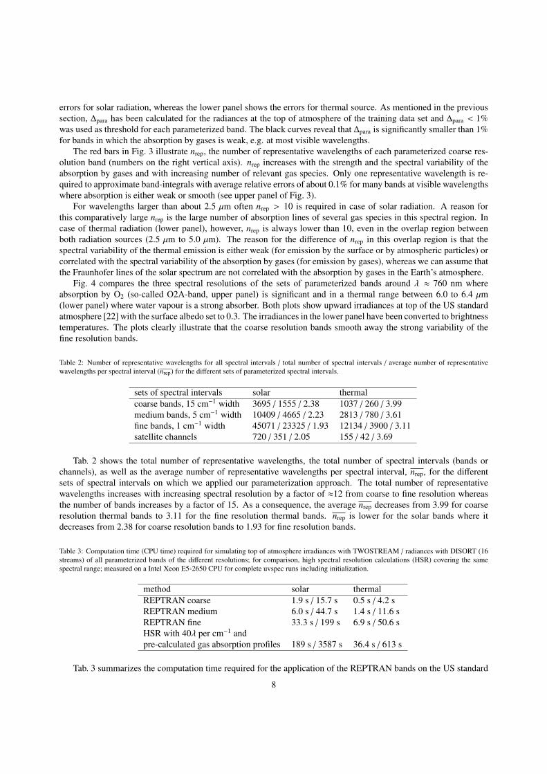
Table 2: Number of representative wavelengths for all spectral intervals / total number of spectral intervals / average number of representativewavelengths per spectral interval (nrep) for the different sets of parameterized spectral intervals.

sets of spectral intervals solar thermalcoarse bands, 15 cm−1 width 3695 / 1555 / 2.38 1037 / 260 / 3.99medium bands, 5 cm−1 width 10409 / 4665 / 2.23 2813 / 780 / 3.61fine bands, 1 cm−1 width 45071 / 23325 / 1.93 12134 / 3900 / 3.11satellite channels 720 / 351 / 2.05 155 / 42 / 3.69

Tab. 2 shows the total number of representative wavelengths, the total number of spectral intervals (bands orchannels), as well as the average number of representative wavelengths per spectral interval, nrep, for the differentsets of spectral intervals on which we applied our parameterization approach. The total number of representativewavelengths increases with increasing spectral resolution by a factor of ≈12 from coarse to fine resolution whereasthe number of bands increases by a factor of 15. As a consequence, the average nrep decreases from 3.99 for coarseresolution thermal bands to 3.11 for the fine resolution thermal bands. nrep is lower for the solar bands where itdecreases from 2.38 for coarse resolution bands to 1.93 for fine resolution bands.

Table 3: Computation time (CPU time) required for simulating top of atmosphere irradiances with TWOSTREAM / radiances with DISORT (16streams) of all parameterized bands of the different resolutions; for comparison, high spectral resolution calculations (HSR) covering the samespectral range; measured on a Intel Xeon E5-2650 CPU for complete uvspec runs including initialization.

method solar thermalREPTRAN coarse 1.9 s / 15.7 s 0.5 s / 4.2 sREPTRAN medium 6.0 s / 44.7 s 1.4 s / 11.6 sREPTRAN fine 33.3 s / 199 s 6.9 s / 50.6 sHSR with 40λ per cm−1 andpre-calculated gas absorption profiles 189 s / 3587 s 36.4 s / 613 s

Tab. 3 summarizes the computation time required for the application of the REPTRAN bands on the US standard

8

0

50

100

150

200

250

300

350

400

758 760 762 764 766 768

up

ward

irr

ad

iance

[m

W m

-2 b

and

-1]

wavelength [nm]

coarsemedium

fine

220

225

230

235

240

245

6000 6050 6100 6150 6200 6250 6300 6350 6400

bri

ghtn

ess

tem

pera

ture

[K

]

wavelength [nm]

coarsemedium

fine

Figure 4: Comparison of spectral resolutions of the parameterized bands around the O2A absorption band (upper panel) and a thermal range (lowerpanel).

9

atmosphere [22] without aerosol or clouds and the complete spectral range they have been created for. The compu-tation times are for complete uvspec runs, including initialization etc. The REPTRAN bands have been applied forthe simulation of top of atmosphere irradiances using the TWOSTREAM solver [23] and top of atmosphere radiancesusing the DISORT solver [16]. For comparison, high spectral resolution calculations (HSR) have been performedon the same spectral range using a spectral resolution of 40 monochromatic simulations per cm−1. The absorptioncoefficients for the HSR calculations have been calculated using ARTS (computation times of ARTS not consideredin Tab. 3) and were then used as input to the uvspec model for simulating the irradiances and radiances. Simulatingirradiances within all coarse resolution solar bands (15 cm−1 width) from 395 nm to 5000 nm requires 1.9 s of compu-tation time (single-threaded) on a Intel Xeon E5-2650 CPU; the computational cost increases with increasing spectralresolution, approximately proportionally with the number of bands. The computational cost increases by a factor of 6to 8 when radiances are simulated instead of irradiances. In case of HSR calculations with 40 lines per cm−1, the com-putation time requirement increases by a factor of about 5 to 20 compared with the fine resolution REPTRAN bandsif the spectral absorption coefficients have been pre-calculated. The computation time requirement for simulations ofthe thermal bands is approximately one quarter of the requirement for the solar bands. The reduction of computationtime for REPTRAN as compared with HSR, which can be up to several orders of magnitude, mainly depends on theselected spectral resolutions of REPTRAN and HSR and whether the gas absorption coefficients are already availablefor HSR calculations or are yet to be calculated.

The average value of nrep over all parameterized satellite instrument channels is about 2 for solar source and 3.7for thermal source (Tab. 2). The low number of radiative transfer calculations required to simulate channel-integratedradiances results in very low computational times for the parameterized channels. For example, a uvspec simulation ofradiances at the parameterized 3.9 µm channel of SEVIRI (nrep = 8), using the DISORT solver and thermal radiation,takes 0.105 s on a PC. Using the LOWTRAN parameterization with a spectral resolution of 5 cm−1 takes 9.1 s for thesame channel.

3.2. Absorption by gas species

Direct transmittances of different gas species considered by uvspec are shown in Fig. 5 as function of wavelength.Here, the transmittance of a species is the fraction of the incoming sunlight (with the sun at zenith) that passes throughthe US standard atmosphere [22] to the surface; all other species are removed from the atmospheric setup. Scatteringis switched off. Note the reversed logarithmic scale for ’1 - transmittance’, i.e. the absorbed fraction of the incidentlight, on the vertical axes in Fig. 5. The upper panel shows the data for λ < 850 nm, whereas the lower panel showsthe data for λ > 850 nm. The data has been calculated using the parameterized solar coarse resolution bands with theabsorption calculated as described in Sect. 2.3. Water vapour absorption (red) is significant in most bands in the nearinfrared; absorption by O2 is significant mainly in the O2A band around λ = 760 nm. The lower panel shows thatabsorption by CO2 and CH4 becomes increasingly relevant for about λ ≥ 1.4 µm.

Fig. 6 shows the transmittance of the different species of the US standard atmosphere calculated using the pa-rameterized thermal coarse resolution bands. The upper panel of Fig. 6 shows transmittances for the main absorbers,whereas the lower panel shows data for the minor absorbers. The absorption by water vapour (red line in upper panelof Fig. 6) is strong (virtually no transmittance) in large parts of the thermal spectrum, except from about 3.4 µm to 4.8µm and from about 8 µm to 15 µm. Within these wavelength ranges, absorption by CO2, and to a minor extent alsoabsorption by CH4, O3, N2O, N2, and CO is relevant.

3.3. Parameterized satellite channels

We have applied the REPTRAN parameterization approach to almost 400 satellite channels (Appendix A). Theparameterization data (λirep and wirep ) for the channels of the Spinning Enhanced Visible and Infrared Imager (SEVIRI)on the MSG3 satellite is provided in Appendix B. For validation of REPTRAN, we now compare modeling resultsfor the parameterized MSG3 channels with respective results from HSR calculations.

Tab. 4 shows mean (maximum) deviations of the parameterized channels from HSR calculations for radiances attop of atmosphere. Four solar channels of SEVIRI are considered. The deviations were averaged over 12 atmospheresand 10 viewing directions (cosines of viewing zenith angle equidistant from 0.1 to 1.0) for each atmosphere. The 12atmospheres did not contain aerosols nor clouds and the sun is at zenith. The atmospheric set included 6 standardatmospheres [22] and 6 randomly chosen atmospheres from an ECMWF data set that has been optimized for large

10

0.999

0.99

0.9

0.0400 450 500 550 600 650 700 800

transm

itta

nce

wavelength [nm]

H2OO2O3

NO2

0.999

0.99

0.9

0.0900 1000 1200 1500 2000 2500

transm

itta

nce

wavelength [nm]

H2OO2

CO2CH4

Figure 5: Transmittance of absorbing species through the US standard atmosphere from λ = 395 nm to 850 nm (upper panel) and 850 nm to 2500nm (lower panel), calculated using the parameterized solar coarse resolution bands; for clarity, the transmittance of O3, N2O, and CO is not shownis the lower panel, though it is between 0.999 and 0.99 for some bands (and > 0.999 elsewhere).

11

0.999

0.99

0.9

0.02500 3000 4000 5000 7000 10000 20000 100000

transm

itta

nce

wavelength [nm]

H2OCO2CH4

0.999

0.99

0.9

0.02500 3000 4000 5000 7000 10000 20000 100000

transm

itta

nce

wavelength [nm]

O2O3N2

N2OCO

Figure 6: Analogous to Fig. 5, but for thermal bands.

12

Table 4: Root mean squared relative deviations (maximum) of radiances within solar satellite channels, averaged over 10 viewing angles and 12atmospheres (see text for details); the surface albedo is set to 0.3.

channel REPTRAN - HSR LOWTRAN - HSRmsg3 seviri ch006 0.30% (0.68%) 0.96% (1.43%)msg3 seviri ch008 0.44% (1.62%) 1.79% (7.64%)msg3 seviri ch016 0.51% (1.09%) 4.02% (18.3%)msg3 seviri ch039 0.35% (1.28%) 9.93% (47.1%)

Table 5: Root mean squared deviations (maximum) for radiance brightness temperatures within thermal satellite channels, averaged over 10different viewing angles and 12 atmospheres (see text for details); the surface albedo is set to 0.0.

channel REPTRAN - HSR LOWTRAN - HSRmsg3 seviri ch039 0.10 K (0.31 K) 0.50 K (1.59 K)msg3 seviri ch062 0.21 K (0.82 K) 0.57 K (0.92 K)msg3 seviri ch073 0.27 K (0.76 K) 1.87 K (2.90 K)msg3 seviri ch087 0.22 K (0.45 K) 0.40 K (1.17 K)msg3 seviri ch097 0.35 K (0.78 K) 2.08 K (7.51 K)msg3 seviri ch108 0.09 K (0.23 K) 0.40 K (1.14 K)msg3 seviri ch120 0.17 K (0.31 K) 0.50 K (1.22 K)msg3 seviri ch134 0.39 K (0.96 K) 3.76 K (7.15 K)

variability of temperature [24]. The N2, N2O, CH4, and CO mixing ratio profiles from the US standard atmospherewere used in all 12 atmospheres. Rayleigh scattering and a surface albedo of 0.3 were considered in all simulationsfor Tab. 4. The high spectral resolution calculations (HSR) for each channel were performed at 12200 wavelengthswithin the channel boundaries. A spectral resolution of 1 nm was used for the LOWTRAN calculations.

The average relative deviation of REPTRAN from HSR is lower than 1% for all channels when averaged overthe 12 atmospheres and 10 viewing directions, with a maximum deviation of 1.62%. The deviations of LOWTRANfrom HSR are significantly larger with average values between 1% and 10%. Large deviations are found for the3.9 µm channel both for the standard and the ECMWF atmospheres, with a maximum value of 47% for the tropicalatmosphere at high viewing zenith angle.

For eight thermal channels of SEVIRI, mean (maximum) deviations of brightness temperatures at top of atmo-sphere are given in Tab. 5. The mean deviations of the brightness temperatures of REPTRAN from exact HSRcalculations are between 0.09 K and 0.39 K, depending on the channel, with a maximum deviation of 0.96 K for the13.4 µm channel. The mean deviations of LOWTRAN from HSR are between 0.40 K and 3.76 K with a maximumdeviation of 7.51 K for the 9.7 µm channel. The deviations of LOWTRAN from HSR are a factor of about 2 to 9 largerthan the deviations of REPTRAN from the exact method. We point out that REPTRAN satellite channels require avery low number of monochromatic radiative transfer calculations (on average 2-4, see Tab. 2) which results in a verylow computation time for which an example was already given in Sect. 3.1.

3.4. Parameterized bands applied for top of atmosphere irradiances

We model top of atmosphere irradiances using REPTRAN bands and compare these irradiances with equivalentband-integrated irradiances from exact HSR calculations. As described above, the REPTRAN approach has beenoptimized for radiances at the top of atmosphere. The simulations evaluated in the following consider also atmo-spheres which were not considered by the training data set; most atmospheric parameters, however, are within therange spanned by the training data set. We apply the parameterized coarse resolution bands, which are characterizedby a spectral width of 15 cm−1. In case of HSR, the simulations are performed analogous to those performed for thetraining data set (Sect. 2.1.2), except that we increased the spectral resolution by about 50% to 180 per cm−1 in orderto test also the sufficiency of the spectral resolution we used for our training data set. LOWTRAN is considered using

13

-4

-3

-2

-1

0

1

2

3

4

900 1000 1200 1500 2000 3000 5000devia

tion o

f up

ward

irr

ad

iance

[m

W m

-2 b

and

-1]

wavelength [nm]

REPTRAN - HSR±1% relative irradiance deviation

Figure 7: Deviations of the upward irradiances at top of the US standard atmosphere of the parameterized solar bands from high spectral resolutioncalculations (black line); surface albedo is set to 0.3.

a spectral resolution of 1 per cm−1 for the radiative transfer calculations and using, for solar bands, the full resolutionsolar spectrum from Kurucz [17].

3.4.1. Solar bandsWe compare the upward irradiance at top of atmosphere modeled in the solar spectral range using the different

methods. First, we investigate results for the US standard atmosphere [22] without clouds or aerosols. The deviationof the upward irradiance of REPTRAN bands from HSR calculations for this atmosphere is shown for λ ≥ 850 nmas the black line in Fig. 7. The surface albedo is set to 0.3. The thin gray lines illustrate, for comparison, absolutedeviations for 1% relative deviation from the absolute irradiances. Bands with strong gas absorption are characterizedby low absolute irradiances thus the distance between both gray lines is small for such bands. For example, thewater vapour absorption band around λ = 950 nm is clearly visible for the gray lines in Fig. 7. The deviations ofREPTRAN results from the exact HSR calculations are small with maximum values of less than 4 mW m−2 band−1.The comparisons of the black line with the gray lines shows that the relative error of the parameterization is below1% for most bands.

Tab. 6 shows mean and maximum deviations between REPTRAN and HSR for top of atmosphere upward irradi-ances from the same atmospheres as in Sect. 3.3. The wavelength range from 395 nm to 5 µm is considered usingthe coarse band resolution. Tab. 6 reveals that the deviations of REPTRAN bands from the exact HSR calculationsare of comparable magnitude for all investigated atmospheres. This is a strong indication that our training data set issufficient to cover a wide range of atmospheric states. The deviations of LOWTRAN, also shown in Tab. 6, are morethan one order of magnitude larger than the deviations of REPTRAN, independent of the atmospheric state.

The uncertainties of transmittances, i.e. the ratios between the upward irradiances and the incoming solar irradi-ances, calculated using the REPTRAN bands (not shown) are higher than the uncertainties of the upward irradiances.The reason for the increased uncertainty of transmittances is that the representative wavelengths were not directlyoptimized for an accurate parameterization of the incoming solar irradiance. The root mean squared relative devia-

14

Table 6: Root mean squared (maximum) deviations between the calculation methods for upward irradiances at top of different atmospheres [22, 24]for solar coarse bands in the spectral range from 395 nm to 5 µm; the unit is mW m−2 band−1; surface albedo is set to 0.3.

atmosphere REPTRAN - HSR LOWTRAN - HSRUS standard 0.588 (3.86) 11.5 (97.1)subarctic winter 0.615 (4.68) 10.6 (98.9)subarctic summer 0.553 (3.01) 12.0 (96.7)midlatitude winter 0.581 (5.00) 11.1 (98.3)midlatitude summer 0.577 (3.30) 12.6 (96.3)tropical 0.622 (3.60) 13.3 (96.3)6 ECMWF atmospheres 0.696 (5.39) 10.1 (98.9)

tion between REPTRAN and HSR for the band-integrated incoming solar irradiances is on the order of 1.3% with amaximum deviation of 13.8%. The relative deviations for transmittances are of comparable magnitude.

3.4.2. Thermal bandsBefore we compare REPTRAN with other methods in the thermal spectral range, we investigate two sources

for deviations: First, differences in the model layer optical depth calculations are relevant when comparing top ofatmosphere irradiances in the thermal range. For example, the data of the standard atmospheres [22] is available at a5 km height resolution for heights above 50 km, thus model layers are 5 km thick. In case of high spectral resolutioncalculations (HSR), we calculate the gas absorption profiles with ARTS and use them in uvspec. For export to uvspec,the current version of ARTS uses

τHSR =Cabs(ztop) · n(ztop) + Cabs(zbottom) · n(zbottom)

2· (ztop − zbottom) (5)

to calculate the layer optical depth for each gas species and model atmosphere layer from zbottom to ztop. In case ofREPTRAN and LOWTRAN, by default the following formula is used by uvspec:

τuvspec =Cabs(ztop) + Cabs(zbottom)

2·

n(ztop) + n(zbottom)2

· (ztop − zbottom) (6)

Here, Cabs is the absorption cross section (depending on p, T , xH2O) at height z, and n the number density of the gasspecies at height z. Fig. 8 illustrates the brightness temperature deviations due to the difference between both formulasfor top of atmosphere upward irradiances. The deviation due to the different formulas is larger than 0.1 K for manybands, reaching values up to 0.3 K. The thin gray lines illustrate the deviation of the brightness temperature when theirradiance deviates by ±1%. Comparison of the black and gray lines shows that the relative deviation of the irradianceis on the order of 2% for λ < 3 µm and 1% or smaller elsewhere. To exclude deviations due to different layer opticaldepth formulas, we perform the REPTRAN and LOWTRAN calculations using Eq. 5 instead of the default Eq. 6 inthe remainder of this section.

A second source for deviations is the fact that the training data set used for parameterizing the bands consists ofatmospheres with top heights around 65 km, but the heights of the standard atmospheres [22], which are included inthe libRadtran package and used in the current section, are 120 km. The pressure and temperature conditions at z > 65km may result in spectral absorption features that were not considered when parameterizing the spectral bands. Fig. 9compares the deviation of REPTRAN from HSR for the US standard atmosphere with a top height of 120 km (black)and the same atmosphere cut at a height of 60 km (green). This “top height effect” is relevant at wavelengths werethe green line is visible in this figure. These wavelengths are characterized by non-negligible gas absorption at thehigh altitudes. Absorption by CO2 is relevant at around 2.7 µm, 4.3 µm and 15 µm, whereas absorption by O3 andH2O is relevant at the other spectral regions where the green line is visible in Fig. 9. While the maximum deviationof REPTRAN from HSR is slightly larger than 0.5 K when the height of the atmosphere is only 60 km, the maximumdeviation increases to about 1 K (or about 5% of the irradiance) when the height of the atmosphere is 120 km. This“top height effect” is not compensated in the following since we use the complete atmospheric profiles (extending toheights of 120 km for all standard atmospheres and about 78 km for the ECMWF atmospheres).

15

-3

-2

-1

0

1

2

3

2500 3000 4000 5000 7000 10000 20000 100000

devia

tion o

f b

rig

htn

ess

tem

p.

[K]

wavelength [nm]

deviation due to layer optical depth formula±1% relative irradiance deviation

Figure 8: Deviations of brightness temperatures of upward irradiances at the top of the US standard atmosphere due to different layer optical depthformulas [Eq. 5 vs. Eq. 6] using REPTRAN thermal bands (black line); the surface albedo is set to 0.

16

-3

-2

-1

0

1

2

3

2500 3000 4000 5000 7000 10000 20000 100000

devia

tion o

f b

rig

htn

ess

tem

p. [K

]

wavelength [nm]

REPTRAN - HSR (at z=60km)REPTRAN - HSR (at TOA)

±1% relative irradiance deviation

Figure 9: Deviations of brightness temperatures of upward irradiances at top of US standard atmosphere between REPTRAN parameterization andhigh spectral resolution calculations (HSR); the black line considers the complete profile up to z = 120 km, whereas the green line considers onlyheights up to z = 60 km; the surface albedo is set to 0.

17

Table 7: Root mean squared deviations (maximum) between the methods for brightness temperatures of upward irradiances in the thermal spectralrange at top of different atmospheres; the surface albedo is set to 0.0.

atmosphere REPTRAN - HSR LOWTRAN - HSRUS standard 0.17 K (0.95 K) 2.86 K (10.6 K)subarctic winter 0.17 K (0.80 K) 1.70 K (6.0 K)subarctic summer 0.17 K (0.97 K) 2.55 K (9.0 K)midlatitude winter 0.16 K (0.75 K) 2.19 K (7.9 K)midlatitude summer 0.16 K (0.95 K) 2.80 K (9.4 K)tropical 0.15 K (0.82 K) 2.99 K (9.6 K)6 ECMWF atmospheres 0.21 K (1.60 K) 1.99 K (9.2 K)

Table 8: Root mean squared (maximum) deviations between the methods for direct solar irradiance at the surface for different atmospheres; theunit is mW m−2 band−1.

atmosphere REPTRAN - HSR LOWTRAN - HSRUS standard 3.21 (20.3) 26.7 (199)subarctic winter 2.57 (13.4) 23.2 (204)subarctic summer 2.89 (18.8) 28.5 (198)midlatitude winter 2.90 (20.7) 25.0 (202)midlatitude summer 2.93 (17.1) 30.5 (208)tropical 2.77 (17.6) 32.8 (231)6 ECMWF atmospheres 2.93 (32.1) 22.8 (204)

After the inspection of two sources for deviations we now focus on the actual deviations of REPTRAN thermalbands from exact HSR results. The deviation of REPTRAN from HSR for the complete US standard atmosphere istypically on the order of 0.1 K, with maximum values close to 1.0 K (see black line in Fig. 9). The larger deviationsoccur mainly for bands where the described “top height effect” is relevant.

Tab. 7 shows mean and maximum deviations of REPTRAN from HSR for different atmospheric states. Thedeviations for most atmospheres are comparable with the deviations found for the US standard atmosphere, wherebyslightly enhanced deviations are found for the ECMWF atmospheres. As mentioned above, the ECMWF atmospheresare characterized by a strong variability of temperature profiles. The deviations of LOWTRAN from HSR, also shownin Tab. 7, are approximately one order of magnitude larger than the deviations of REPTRAN from HSR.

3.5. Parameterized bands applied for surface irradiances

After investigating irradicances at the top of atmosphere, we now apply coarse bands parameterized with REP-TRAN for simulating irradiances at the surface. We perform comparisons to exact HSR calculations analogous tothe comparisons performed for the top of atmosphere. The application of REPTRAN at the surface potentially couldresult in large errors because the parameterized bands have been optimized for top of atmosphere radiances and mightnot capture spectral absorption features relevant at lower atmospheric levels. This issue will be investigated in thefollowing.

3.5.1. Solar bandsTab. 8 summarizes deviations of the parameterized band-integrated direct solar irradiances at the surface. The root

mean squared deviations together with the maximum deviations are given for the coarse resolution bands. The meandeviation of REPTRAN from HSR does not vary significantly between the atmospheres and is close to 3 mW m−2

band−1 with maximum values of 32.1 mW m−2 band−1 for an ECMWF atmosphere. The mean relative deviation ofREPTRAN from HSR is approximately 0.45% of the mean solar irradiance at the surface (≈ 650 mW m−2 band−1).At top of atmosphere, the mean relative deviation of the upward irradiance (≈ 0.6 mW m−2 band−1, Tab. 6) is ap-proximately 0.3% of the mean upward irradiance (≈ 200 mW m−2 band−1). This indicates that the relative error for

18

-3

-2

-1

0

1

2

3

4

2500 3000 4000 5000 7000 10000 20000 100000

devia

tion o

f b

rig

htn

ess

tem

p. [K

]

wavelength [nm]

REPTRAN - HSR±1% relative irradiance deviation

Figure 10: Deviations of brightness temperatures of downward irradiances at the surface of the US standard atmosphere; surface albedo is set to0.0.

irradiances calculated using REPTRAN is only slightly larger at the surface than at the top of atmosphere. The goodperformance for solar irradiance at the surface is probably a result of the fact that most of the upward irradiance attop of atmosphere has been reflected by the surface and thus, like the irradiance at the surface, contains the spectralinformation from all atmospheric layers. The deviations of LOWTRAN from HSR are approximately one order ofmagnitude larger than the deviations found for REPTRAN, confirming that the REPTRAN parameterization performscomparatively well for solar irradiance at the surface, though it was not optimized for this setup.

3.5.2. Thermal bandsAs the next step, we consider brightness temperatures of thermal downward irradiances reaching the surface.

Fig. 10 shows deviations of brightness temperatures calculated using REPTRAN coarse thermal bands for the USstandard atmosphere from exact HSR calculations. The deviations are largest at wavelengths where the brightnesstemperature is low. The deviation of REPTRAN from HSR reaches maximum values close to 3.5 K around λ =

10 µm. Comparison of the black line with the gray lines (1% lines) indicates that the maximum relative deviationof REPTRAN from HSR is on the order of 10%. There are some systematic deviations at wavelengths with strongabsorption, mainly between 5 µm and 7.5 µm and wavelengths larger 40 µm. These deviations might be related tothe difference of the spectral slopes of the radiances from blackbodies either having the temperature of the surface orthe temperature of the uppermost atmospheric layers and the fact that the representative wavelengths for bands withstrong absorption were selected to consider the spectral slope of the latter. Nonetheless, the relative deviation of thethermal irradiance at the surface is below 1% for a large fraction of bands.

Tab. 9 shows the root mean squared and maximum deviations of the brightness temperatures at the surface fordifferent atmospheres. The deviations of all standard atmospheres are comparable with the deviations found for theUS standard atmosphere. The deviations are slightly larger for the ECMWF atmospheres than for the standard at-mospheres. A comparison of the brightness temperature deviations at the top of atmosphere (Tab. 7) and the surface(Tab. 9) reveals that the mean deviations of REPTRAN from HSR are approximately three times larger at the sur-

19

Table 9: Root mean squared (maximum) deviations between the methods for brightness temperatures of downward irradiances at the surface fordifferent atmospheres; surface albedo is set to 0.0.

atmosphere REPTRAN - HSR LOWTRAN - HSRUS standard 0.61 K (3.47 K) 3.83 K (13.8 K)subarctic winter 0.58 K (2.96 K) 3.97 K (12.3 K)subarctic summer 0.53 K (3.11 K) 3.29 K (11.5 K)midlatitude winter 0.60 K (2.64 K) 3.73 K (13.0 K)midlatitude summer 0.56 K (3.55 K) 3.29 K (11.7 K)tropical 0.57 K (3.51 K) 3.23 K (11.7 K)6 ECMWF atmospheres 0.73 K (4.46 K) 4.29 K (14.9 K)

face than at the top of atmosphere. The mean deviations of LOWTRAN from HSR are typically 6-7 times largerthan the deviations of REPTRAN from the HSR, showing a comparatively good accuracy of REPTRAN for thermalcalculations also at the surface.

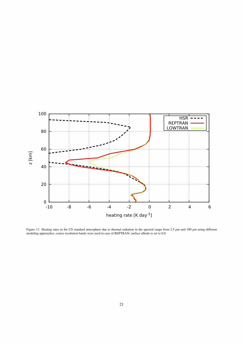
3.6. Parameterized bands applied for heating ratesFig. 11 compares heating rate profiles calculated using the different approaches. It shows spectrally-integrated

heating rates for thermal radiation in the wavelength range from 2.5 to 100 µm. The agreement between the ap-proaches is reasonably good below 20 km with maximum deviations in the range of 0.2 K per day. The REPTRANand LOWTRAN parameterizations however deviate significantly from HSR at high altitudes, in particular at heights z> 40 km. The main reason for the deviations at high altitudes is that the gas absorption spectrum contains very narrowand strong absorption lines at these altitudes which are captured by HSR calculations but not by the parameterizations.These very narrow and strong absorption lines are hardly relevant for spectrally-integrated radiances but have largeeffect on spectrally-integrated heating rates. Thus, for the representative wavelengths parameterization approach itseems plausible to assume that wavelengths with such strong absorption lines are hardly selected as representativewavelengths since the presented approach optimizes for radiances. Fig. 11 illustrates that neither REPTRAN norLOWTRAN should be used for calculating heating rates at high altitudes. Using REPTRAN fine resolution bandsinstead of coarse bands does not significantly reduce the deviations of REPTRAN from HSR. Respective results forspectrally-integrated heating rates in the solar spectral range (not shown here) revealed a comparable height depen-dence of the deviations, that is only small deviations at lower altitudes and large deviations at high altitudes.

4. Conclusions

We adopted and optimized the representative wavelengths approach of Buehler et al. [11] for parameterizingspectral bands of different widths (1 cm−1, 5 cm−1, and 15 cm−1), as well as for parameterizing spectral responsefunctions of a large number of satellite channels. Solar as well as thermal radiation up to λ = 100 µm was considered.The parameterization approach considers gas absorption lines from the HITRAN spectroscopic data set in additionto continuum absorption from the MT CKD model. It optimizes for spectrally-integrated radiances at the top ofatmosphere with an accuracy threshold of 1% for a large set of highly variable states of the Earth’s atmosphere. Weimplemented the parameterized bands and satellite channels as a new parameterization option (named “REPTRAN”)in the freely available uvspec model and compared results from this implementation with results from high spectralresolution (HSR) calculations. We also compared results from the already-implemented LOWTRAN parameterizationwith HSR calculations.

From the application of REPTRAN it was found that:

1. Only few representative wavelengths are required to parameterize spectral integrals. Typically less than 10, andon average about 3 representative wavelengths are sufficient to fulfill the radiance accuracy threshold of 1%.The number of required wavelengths is largest (up to 22) in case of solar radiation and wavelengths larger than2 µm (Fig. 3).

2. The uncertainty of REPTRAN for modeling of satellite channel responses is low (Tabs. 4, 5).

20

0

20

40

60

80

100

-10 -8 -6 -4 -2 0 2 4 6

z [k

m]

heating rate [K day-1]

HSRREPTRAN

LOWTRAN

Figure 11: Heating rates in the US standard atmosphere due to thermal radiation in the spectral range from 2.5 µm and 100 µm using differentmodeling approaches; coarse resolution bands were used in case of REPTRAN; surface albedo is set to 0.0.

21

3. The comparisons for spectral bands revealed that the uncertainty of REPTRAN is low for both solar and thermalupward irradiance at the top of atmosphere as well as for solar irradiance at the surface (Tabs. 6, 7, 8).

4. The uncertainty of REPTRAN for thermal downward irradiance at the surface is higher than for thermal ir-radiance at the top of atmosphere, on average by a factor of 3. Nevertheless, the uncertainty of REPTRANfor thermal irradiance at the surface is still significanty lower than the uncertainty of the already-implementedparameterization (Tab. 9).

5. The uncertainty of thermal heating rates is comparable for REPTRAN and LOWTRAN. While the maximumdeviations are in the range of 0.2 K per day in the troposphere and the lower stratosphere, significantly largerdeviations from HSR calculations are found for both parameterizations at altitudes above 20 km (Fig. 11).The large deviations of REPTRAN can be understood as a result of its optimization for spectrally-integratedradiances and the fact that absorption lines at high altitudes are comparatively narrow and strong, affecting thespectrally-integrated heating rates much stronger than spectrally-integrated radiances.

When adding a new constituent to the atmospheric setup, the results from the application of the presented REP-TRAN data might become unpredictable if the constituent exhibits a strong spectral variability that was not consideredwhen parameterizing the spectral intervals. In most other cases, however, the presented REPTRAN parameterizationapproach provides quite low uncertainty for radiative transfer modeling of the Earth’s atmosphere. Furthermore, it re-duces significantly the computation time requirements compared with other approaches, in particular when modelingradiances of satellite radiometers. The REPTRAN parameterization data files for bands as well as satellite channelsare provided at the libRadtran webpage - http://libradtran.org.

Acknowledgements

This study was funded by ESTEC under Contract AO/1-6607/10/NL/LvH (ESASLight II project). Spectral re-sponse functions of satellite instrument channels were provided by ESA.

Appendix A. List of parameterized satellite channel response functions

A list of parameterized satellite channels for solar radiation is given in Tab. A.10; channels parameterized forthermal radiation are given in Tab. A.11.

Appendix B. List of representative wavelengths for MSG3 channels

A list of representative wavelengths and weights for the channels of the MSG3 SEVIRI instrument is given forsolar radiation source in Tab. B.12 and for thermal radiation source in Tab. B.13. They can be applied together with theabsorption data described above. Representative wavelengths, their weights, and supplementary data can be extractedfrom the data available from the libRadtran webpage for any parameterized channel and band.

22

Table A.10: Satellite channel response functions parameterized for solar radiation.

satellite instrument channel nameADEOS1 POLDER 443np 443p1 443p2 443p2 490np 565np 670p1

670p2 670p3 763np 765np 865p1 865p2 865p3 910npADEOS2 POLDER 443 443p 490 565 670p 763 765 865p 910ALOS AVNIR2 b1 b2 b3 b4EarthCARE MSI b1 b2 b3 b4Envisat AATSR ir37 v16 v555 v659 v870Envisat MERIS ch01 . . . ch15ERS1 ATSR ir36 v16ERS2 ATSR ir36 v16 v555 v659 v870Landsat1 . . . Landsat5 MSS b1 b2 b3 b4Landsat4 Landsat5 TM b1 b2 b3 b4 b5 b7Landsat7 ETM b1 b2 b3 b4 b5 b7 b8MSG1 MSG2 MSG3 SEVIRI ch006 ch008 ch016 ch039PARASOL POLDER 1020 443 490 565 670 763 765 865 910PROBA CHRIS a01 . . . a61, c01 . . . c18, h01 . . . h37

l01 . . . l18, l01a . . . l18a, w01 . . . w18Sentinel3 OLCI b02 . . . b21Sentinel3 SLSTR b1 . . . b7Seosat b1 b2 b3 b4SPOT1 SPOT2 SPOT3 HRV b1 b2 b3 panSPOT4 HRVIR b1 b2 b3 b4 monoSPOT4 VEGETATION1 b0 b2 b3 b4SPOT5 HRG b1 b2 b3 b4 panSPOT5 VEGETATION2 b0 b2 b3 b4

Table A.11: Satellite channel response functions parameterized for thermal radiation.

satellite instrument channel nameEarthCare MSI b7 b8 b9Envisat AATSR ir11 ir12 ir37ERS1 ERS2 ATSR ir11 ir12 ir37Landsat4 Landsat5 TM b6Landsat7 ETM b6MSG1 MSG2 MSG3 SEVIRI ch039 ch062 ch073 ch087 ch097 ch108 ch120 ch134Sentinel3 SLSTR b7 b8 b9

23

Table B.12: Representative wavelengths λirep and weights wirep optimized for different satellite channels and solar radiation source.

channel irep λirep [nm] wirep solar flux [mW m−2 nm−1]msg3 seviri ch006 1 619.5815 0.586 1655

2 664.4795 0.414 1567msg3 seviri ch008 1 796.2853 0.208 1129

2 806.4738 0.792 1089msg3 seviri ch016 1 1584.574 0.134 225.3

2 1639.934 0.459 228.83 1652.107 0.228 229.94 1684.948 0.179 212.9

msg3 seviri ch039 1 3607.132 0.013 12.992 3621.609 0.046 12.823 3660.757 0.037 12.304 3683.176 0.034 11.945 3692.384 0.018 11.856 3787.928 0.143 10.777 3794.640 0.066 10.728 3806.782 0.028 10.589 3879.779 0.105 9.8410 3995.603 0.226 7.6011 4111.002 0.283 6.98

24

Table B.13: Representative wavelengths λirep and weights wirep optimized for different satellite channels and thermal radiation source.

channel irep λirep [nm] wirep

msg3 seviri ch039 1 3690.930 0.0992 3704.772 0.2953 3874.026 0.1374 3942.741 0.0195 4005.412 0.2656 4152.224 0.1397 4214.193 0.0368 4237.213 0.009

msg3 seviri ch062 1 6088.564 0.4632 6106.765 0.0703 6536.340 0.467

msg3 seviri ch073 1 7228.371 0.4502 7376.566 0.0613 7481.678 0.2624 7508.143 0.1235 7559.400 0.104

msg3 seviri ch087 1 8574.521 0.2772 8581.394 0.0823 8772.607 0.6214 8835.432 0.020

msg3 seviri ch097 1 9550.629 0.2772 9661.430 0.4313 9716.618 0.2474 9785.438 0.044

msg3 seviri ch108 1 10245.674 0.0962 10831.648 0.904

msg3 seviri ch120 1 11872.122 0.8372 12285.149 0.163

msg3 seviri ch134 1 12839.421 0.3852 13766.827 0.3953 13782.017 0.220

25

References

[1] A. A. Lacis, V. Oinas, A description of the correlated k distribution method for modeling nongray gaseous absorption, thermal emission, andmultiple scattering in vertically inhomogeneous atmospheres, J. Geophys. Res. 96 (1991) 9027–9063. doi:10.1029/90JD01945.

[2] S. Kato, T. Ackerman, J. Mather, E. Clothiaux, The k-distribution method and correlated-k approximation for a shortwave radiative transfermodel, J. Quant. Spectrosc. Radiat. Transfer 62 (1999) 109–121. doi:10.1016/S0022-4073(98)00075-2.

[3] Q. Fu, K. Liou, On the correlated k-distribution method for radiative transfer in nonhomogeneous atmospheres, J. Atmos. Sci. 49 (1992)2139–2156. doi:10.1175/1520-0469(1992)049<2139:OTCDMF>2.0.CO;2.

[4] D. Kratz, The correlated k-distribution technique as applied to the AVHRR channels, J. Quant. Spectrosc. Radiat. Transfer 53 (1995) 501–517.doi:10.1016/0022-4073(95)00006-7.

[5] L. Doppler, R. Preusker, R. Bennartz, J. Fischer, k-bin and k-IR: k-distribution methods without correlation approximation for non-fixedinstrument response function and extension to the thermal infrared - Applications to satellite remote sensing, J. Quant. Spectrosc. Radiat.Transfer 133 (2014) 382–395. doi:10.1016/j.jqsrt.2013.09.001.

[6] F. Kneizys, L. Abreu, G. Anderson, J. Chetwynd, E. Shettle, A. Berk, L. Bernstein, D. Robertson, P. Acharya, L. Rothman, J. Selby,W. Gallery, S. Clough, The MODTRAN 2/3 report and LOWTRAN 7 model, Tech. Rep. Contract F19628-91-C-0132, Phillips Laboratory,Air Force Base, Hanscom (1996).

[7] B. Mayer, A. Kylling, Technical Note: The libRadtran software package for radiative transfer calculations: Description and examples of use,Atmos. Chem. Phys. 5 (2005) 1855–1877. doi:10.5194/acp-5-1855-2005.

[8] L. S. Rothman, D. Jacquemart, A. Barbe, D. Chris Benner, M. Birk, L. R. Brown, M. R. Carleer, C. Chackerian Jr, K. Chance,L. H. Coudert, et al., The HITRAN 2004 molecular spectroscopic database, J. Quant. Spectrosc. Radiat. Transfer 96 (2005) 139–204.doi:10.1016/j.jqsrt.2004.10.008.

[9] S. Wacker, J. Grobner, C. Emde, L. Vuilleumier, B. Mayer, E. Rozanov, Comparison of Measured and Modeled Nocturnal Clear Sky Long-wave Downward Radiation at Payerne, Switzerland, in: T. Nakajima, M. Akemi Yamasoe (Eds.), American Institute of Physics ConferenceSeries, 2009, pp. 589–592. doi:10.1063/1.3117055.

[10] A. Berk, G. P. Anderson, P. K. Acharya, L. S. Bernstein, L. Muratov, J. Lee, M. Fox, S. M. Adler-Golden, J. H. Chetwynd, M. L. Hoke, R. B.Lockwood, J. A. Gardner, T. W. Cooley, C. C. Borel, P. E. Lewis, MODTRAN 5: a reformulated atmospheric band model with auxiliaryspecies and practical multiple scattering options: update, in: Proc. SPIE, Vol. 5806, 2005, pp. 662–667. doi:10.1117/12.606026.

[11] S. Buehler, V. John, A. Kottayil, M. Milz, P. Eriksson, Efficient radiative transfer simulations for a broadband infrared radiometer - combin-ing a weighted mean of representative frequencies approach with frequency selection by simulated annealing, J. Quant. Spectrosc. Radiat.Transfer 111 (2010) 602 – 615. doi:10.1016/j.jqsrt.2009.10.018.

[12] L. Garand, D. S. Turner, M. Larocque, J. Bates, S. Boukabara, P. Brunel, F. Chevallier, G. Deblonde, R. Engelen, M. Hollingshead, D. Jackson,G. Jedlovec, J. Joiner, T. Kleespies, D. S. McKague, L. McMillin, J.-L. Moncet, J. R. Pardo, P. J. Rayer, E. Salathe, R. Saunders, N. A. Scott,P. van Delst, H. Woolf, Radiance and Jacobian intercomparison of radiative transfer models applied to HIRS and AMSU channels, J. Geophys.Res. 106 (2001) 24017 – 24031. doi:10.1029/2000JD000184.

[13] J. R. Key, P. Yang, B. A. Baum, S. L. Nasiri, Parameterization of shortwave ice cloud optical properties for various particle habits, J. Geophys.Res. 107 (2002) 4181. doi:10.1029/2001JD000742.

[14] P. Eriksson, S. Buehler, C. Davis, C. Emde, O. Lemke, ARTS, the atmospheric radiative transfer simulator, version 2, J. Quant. Spectrosc.Radiat. Transfer 112 (2011) 1551 – 1558. doi:10.1016/j.jqsrt.2011.03.001.

[15] S. Clough, M. Shephard, E. Mlawer, J. Delamere, M. Iacono, K. Cady-Pereira, S. Boukabara, P. Brown, Atmospheric radiative transfermodeling: a summary of the AER codes, J. Quant. Spectrosc. Radiat. Transfer 91 (2005) 233 – 244. doi:10.1016/j.jqsrt.2004.05.058.

[16] R. Buras, T. Dowling, C. Emde, New secondary-scattering correction in disort with increased efficiency for forward scattering, J. Quant.Spectrosc. Radiat. Transfer 112 (2011) 2028–2034. doi:10.1016/j.jqsrt.2011.03.019.

[17] R. Kurucz, Synthetic infrared spectra, in: Proceedings of the 154th Symposium of the International Astronomical Union (IAU); Tucson,Arizona, March 2-6, 1992, Kluwer, Acad., Norwell, MA, 1992.

[18] L. Molina, M. Molina, Absolute Absorption Cross Sections of Ozone in the 185- to 350-nm Wavelength Region, J. Geophys. Res. 91 (1986)14501–14508. doi:10.1029/JD091iD13p14501.

[19] G. D. Greenblatt, J. J. Orlando, J. B. Burkholder, A. R. Ravishankara, Absorption measurements of oxygen between 330 and 1140 nm, J.Geophys. Res. 95 (1990) 18577–18582. doi:10.1029/JD095iD11p18577.

[20] J. P. Burrows, A. Dehn, B. Deters, S. Himmelmann, A. Richter, S. Voigt, J. Orphal, Atmospheric remote–sensing reference data from GOME:Part 1. Temperature–dependent absorption cross sections of NO2 in the 231–794 nm range, J. Quant. Spectrosc. Radiat. Transfer 60 (1998)1025–1031. doi:10.1016/S0022-4073(97)00197-0.

[21] S. Buehler, P. Eriksson, O. Lemke, Absorption lookup tables in the radiative transfer model ARTS, J. Quant. Spectrosc. Radiat. Transfer 112(2011) 1559 – 1567. doi:10.1016/j.jqsrt.2011.03.008.

[22] G. Anderson, S. Clough, F. Kneizys, J. Chetwynd, E. Shettle, AFGL Atmospheric Constituent Profiles (0-120 km), Tech. Rep. AFGL-TR-86-0110, AFGL (OPI), Hanscom AFB, MA 01736 (1986).

[23] A. Kylling, K. Stamnes, S.-C. Tsay, A reliable and efficient two–stream algorithm for spherical radiative transfer: documentation of accuracyin realistic layered media , J. of Atmospheric Chemistry 21 (1995) 115–150. doi:10.1007/BF00696577.

[24] F. Chevallier, S. Di Michele, A. P. McNally, Diverse profile datasets from the ECMWF 91-level short-range forecasts, Tech. Rep. NWPSAF-EC-TR-010, European Centre for Medium-Range Weather Forecasts (2006).

26