CHAPTER 1

Representational Measurement Theory .

R. DUNCAN LUCE AND PATRICK SUPPES

CONCEPT OF REPRESENTATIONAL MEASUREMENT

Representational measurement is, on the -one hand, an attempt to understand the nature of empirical observations that can be usefully recoded, in some reasonably unique fashion, in terms of familiar mathematical structures. The most common of these representing struc­tures are the ordinary real numbers ordered in the usual way and with the operations of ad­dition, +, andlor multiplication, .. Intuitively, . such representatious seems a possibility when dealing with variables for which people have a clear sense of "greater than." When data can be summarized numerically, our knowledge of how to calculate and to relate numbers can usefully come into play. However, as we will see, caution must be exerted not to go beyond the information actually coded numerically. In addition, more complex mathematical struc­tures such as geometries are often used, for example, in multidimensional scaling.

On the other hand, representational mea­surement goes well beyond the mereconstruc­tion of numerical representations to a careful examination of how such representations re­late to one another in substantive scientific

The authors thank Janos Aczel. Ehtibar Dzhafarov. Jean­Claude Falmagne, and A.AJ. Marley for helpful com­ments and criticisms of an earlier draft.

1

theories, such as in physics, psychophysics, and utility theory. These may be thought of as applications of measurement concepts for representing various kinds of empirical rela­tions among variables.

In the 75 or so years beginning in 1870, some psychologists (often physicists or phy­sicians turned psychologists) attempted to import measurement ideas from physics, but gradually it became clear that doing this suc­cessfully was a good deal trickier than was initially thought. Indeed, by the 1940s a num­ber of physicists and philosophers of physics concluded that psychologists really did not and could not have an adequate basis for mea­surement. They concluded, correctly, that the classical measurement models were for the most part unsuited to psychological phenom­ena. But they also concluded, incorrectly, that no scientificaJIy sound psychological mea­surement is possible at all. In part, the theory of representational measurement was th~ re- ' sponse of some psychologists and other social scientists who were fairly well trained in the necessary physics and mathematics to under­stand how to modify in substantial ways the classical models of physical measurement to be better suited to psychological issues. The purpose of this chapter is to outline the high points of the 50-year effort from 1950 to the present to develop a deeper understanding of such measurement.

2 Representational Measurement Theory·

Empirical Structures

Performing any experiment, in particular a psychological one, is a complex activity that we never analyze or report completely. The part that we analyze systematically and re­port on is sometimes called a model of the data or, in terms that are useful in the the­ory of measurement, an empirical structure. Such an empirical structure of an experiment is a drastic reduction of the entire experi­mental activity. In the simplest, purely psy­.chological cases, we represent the empirical model as a set of stimuli, a set of responses, 'and some relations observed to hold between the stimuli and responses. (Such an empirical restriction to stimuli and responses does not mean that the theoretical considerations are

so restricted; unobservable concepts may well playa role in theory.) In many psychological measurement experiments such an empirical structure consists of a set of stimuli that vary along a single dimension, for example, a set of sounds varying only in intensity. We might then record the pairwise judgments of loud­ness by a binary relation on the set of stimuli, where the first member of a pair represents the subject's jndgment of which of two sounds was louder:

The use of such empirical structures in psychology is widespread because they come close to the way data are organized for subse­quent statistical analysis or for testing a theory

or hypothesis. An important cluster of objections to the

concept of empirical structures or models of data exists. One is that the formal analysis of empirical structures includes only a small portion of the many problems of experimen­

tal design. Among these are issues such as the randomization of responses between left and right hands and symmetry conditions in the lighting of visual stimuli. For example, in

most experiments that study aspects of vision, having considerably more intense light on the

left side of the subject than on the rigbt would be considered a mistake. Such considerations

do not ordinariI y enter into any formal de­scription of the experiment.· This is just the beginning. There are understood conditions that are assumed to hold but are not enumer· ated: Sudden loud noises did not interfere with the concentration of the subjects, and neither the experimenter talked to the subject nor the subject to the experimenter during the collec­tion of the data-although exceptions to this rule can certainly be found, especially in lin­guistically oriented experiments.

The concept of empirical structures is just meant to isolate the part of the experimental activity and the form of the data relevant to the hypothesis or theory being tested or to the measurements being made.

Isomorphic Strnctures

The prehistory of mathematics, before Babylonian, Chinese, or Egyptian civiliza­tions began, left no written record but none­theless had as a major development the con­cept of number. In particular, counting of small collections of objects was present. Oral terms for some sort of counting seem to exist in every language. The next big step was the introduction, no doubt independently in sev­eral places, of a written notation for numbers. It was a feat of great abstraction to develop the general theory of the constructive opera­tions of counting, adding, subtracting, multi­plying, and Ilividing numbers. The first prob­lem for a theory of measurement was to show how this arithmetic of numbers could be con­structed and applied to a variety of empirical structures.

To investigate this problem, as we do in the next section, we need the general no­

tion of isomorphism between two structures. The intuitive idea is straightforward: Two structures are isomorphic when they exhibit

the same structure from the standpoint of

their basic concepts. The point of the fonnal definition of isomorphism is to make this no­tion of same structure precise.

As an elementary example, consider a binary relational structure consisting of a nonempty set A and a binary relation R de­fined on this set. We will be considering pairs of such structures in which both may be empir­ical structures, both may be numerical struc­tures, or one may be empirical and the other numerical. The definition of isomorphism is unaffected by which combination is being considered.

The way we make the concept of having the same structure precise is to require the ex­

. istence of a function mapping the one struc­ture onto the other that preserves the binary relation. Fonnally, a binary relation structure (A, R) is isomorphic to a binary relation struc­ture (A', R') if and only if there is a function fsuch that

(i) the domain of f is A and the codomain of f is A', i.e., A' is the image of A underJ,

(ii) fis a one-one function,' and

(iii) fora and b inA,aRbiff2 f(a)R'f(b).

To illustrate this definition of isomorph­ism, consider the question: Are any two finite binary relation structures with the same num­ber of elements isomorphic? Intuitively, it seems clear that the answer should be neg­ative, because in one of the structures all the objects could stand in the relation R to each other and not so in the other. This is indeed the case and shows at once, as intended, that isomorphism depends not just on a one-one function from one set to another, but also on the structure as represented in the binary relation.

I In recent years, conditions (i) and (ii) together have come to be called bijective. 2This is a standard abbreviation for "if and only jf:'

Concept of Representational Measurement 3

Ordered Relational Strnctures

Weak Order

An idea basic to measurement.is that the ob­jects being measured exhibit a qualitative at­tribute 'for which it makes sense to ask the question: Which of two objects exhibits more of the attribute, or do they exhibit it to the same degree? For example, the attribute of having greater mass is reflected by placing the two objects on the pans of an equal-arm pan bal­ance and observing which deflects downward. The attribute ofloudness is reflected by which of two sounds a subject deems as louder or equally loud. Thus, the focus of measurement is not just on the numerical representation of any relational structures, but of ordered ones, that is, ones for which one of the relations is a weak order, denoted ~, which has two defin­ing properties for all elements a, b, c in the domain A:

(i) Transitive: if a ~ b and b ~ c, then a ~ c.

(ii) Connected: either a ~ b or b !::; a or both.

The intuitive idea is that!::; captures the order­ing of the attribute that we are attempting to measure.

1\\'0 distinct relations can be defined in tenns of!::;:

a >- biff a~b and not (b!::;a);

a ~ b iff both o!::; b and b~a ..

It is an easy ex~rcise to show that >- is transi­tive and irreflexive (i.e., a >- 0 cannOt hold), and that ~ is an equivalence relation (i.e., transitive. symmetric in the sense that a ""V b iff b ~ a, and reflexive in the sense that a ~ 0). The latter means that ~ partitions A into equivalence classes.

Homomorphism

. For most measurement situations one really is working with weak orders-after all, two entities having the same weight are not in gen- . eral identical. But often it is mathematically

4 Representational Measurement Theory

easier to work with isomorphisms to the or­dered real numbers, in which case one must deal with the following concept of simple or­ders. We do this by inducing the preference order over the equivalence classes defined by "". When""'" is =. each element is an equiva­lence class, and the weak order::: is called a simple order. The mapping from the weakly ordered structure via the isomorphisms of the (mutually disjoint) equivalences classes to the ordered real numbers is called a ho­momorphism. Unlike an isomorphism, which is one to one, an homomorphism is many to one. In some cases, such as additive conjoint m"easurement, discussed later, it is somewhat difficult, although possible, to formulate the theory using the equivalence classes.

fuo Fundamental Problems of Representational Measurement

Existence

The most fundamental problem for a theory of representational measurement is to construct the following representation: Given an empir­ical structure satisfying certain properties, to which numerical structures, if any, is it iso­morphic? These numerical structures, thus, represent the empirical one. It is the existence of such isomorphisms that constitutes the representational claim that measurement of a fundamental kind has taken place.

Quantification or measnrement, in the sense just characterized, is important in some way in all empirical sciences. The primary significance of this fact is that given the iso­morphism of Structures, we may pass from the particular empirical structure to the numerical one and then use all our familiar computa­tional methods, as applied to the isomorphic arithmetical structure, to infer facts about the isomorphic empirical structure. Such passage from simple qUalitative observations to quan­titative ones-the isomorphism of structures

passing from the empirical to the numerical­is necessary for precise prediction or control of phenomena. Of course, such a representa­tion is useful only to the extent of the precision of the observations on which itis based. A va­riety of numerical representations for various empirical psychological phenomena is given in the sections that follow.

Uniqueness

The second fundamental problem of repre­sentational measurement is to discover the uniqueness of the representations. Solving the representation problem for a theory of mea­snrement is not enough. There is usually a formal difference between the kind of assign­meIit of numbers arising from different pro­cedures of measurement. as may be seen in three intuitive examples:

. 1. The populati on of California is greater than that of New York.

2. Mary is 10 years older than John.

3. The temperature in New York City this afternoon will be 92 OF.

Here we may easily distinguish three kinds of measurements. The first is an example of counting, which is an absolute scale. The number of members of a given collection that is counted is determined uniquely in the ideal case, a1\h<iugh that Can be difficult in prac­tice (wituess the 2000 presidential election in Florida). In contrast, the second example, the measurement of difference in age, is a ratio scale. Empirical procedures for mea­suring age do not determine the unit of age-­chosen in the example 10 be the year rather than, for example, the month or the week. Although the choice of the unit of a per­son's age is arbitrary-that is. not empiri­cally prescribed-that of the zero, birth, is not. Thus, the ratio of the ages of any two peo­ple is independent of its choice. and the age of people is an example of a ratio scale. The

measurement of distance is another example of such a ratio scale. The third example, that of temperature, is an example of an interval scale. The empirical procedure of measuring temperature by use of a standard thermometer or other device determines neither a unit nor an origin.

We may thus also describe the second fun­damental problem for representational mea­surement as that of detennining the scale type of the measurements resulting from a given procedure.

A.BRIEF HISTORY OF MEASUREMENT

Pre-19th-Century Measurement

Already by the fifth century B.C., if not before, Greek geometers were.investigatillg problems central to the nature of measurement. The Greek achievements in mathematics are all of relevance to measurement. First, the theory of number, meaning for them the theory of the' positive integers, was closely connected with counting; second, the geometric theory of pro­portion was central to magnitudes that we now represent by rational numbers (= ratios of in­tegers); and, finally, the theory of inc ommen­surable geometric magnitudes fo~ those mag­nitudes that could not be represeuted by ratios. The famous proof of the irrationaJ.ity of the square root of two seems arithmetic in spirit to us, but almost certainly the Greek discov­ery of incommensurability was geometric in character, namely, that the length of the di­agonal of a square, or the hypotenuse of an isosceles right-angled triangle, was not com­mensurable with the sides. The Greeks well understood that the varions kinds of results just described applied in general to magni­tudes and not in any sense only to numbers or even only to the length of line segments. The spirit of this may be seen in the first def­inition of Book 10 of Euclid, the one dealing

A Brief History of Measurement 5"

with incommensurables: "Those magnitudes are said to be cOminensurable which are mea­sured by the same measure, and those incom­mensurable which cannot have any common measure" (trans. 1956, p. 10).

lt does not take much investigation to de­termine that theories and practices relevant to measurement occur throughout the centuries in many different contexts. lt is impossible to give details here, bnt we mention a few salient examples. The first is the discussion

" of the measurement of pleasure and pain in Plato's dialogue Protagoras. The second is the set of partial quaJ.itative axioms, character­izing in our tenns empirical structures, given by Archimedes for measuring on unequal bal­ances (Suppes, 1980). Here the two qualitative concepts are the distance from the focal point of the balance and the weights of the objects placed in the two pans of the balance. This is perhaps the first partial qualitative axiom­atization of conjoint measurement, which is discussed in more detail later. The third ex­ample is the large medieval literature giving a variety of qualitative axioms for the measure­ment of weight (Moody and Claggett, 1952). (psychologisis concerned about the difficulty of clarifying the measurement of fundamen­ta! psychological quantities should be encour­aged by reading O'Brien's 1981 detailed ex­position of the confused theories of weight in the ancient world.) The fourth example is the detailed discussion of intensive quantities by Nicole Oresme in the 14th century A.D. The fifth is GaIileo's successful geometrization in the 17th century of the motion of heavenly

. bodies, done in the context of stating essen':' tially qualitative axioms for what, in the ear­lier tradition, would be called the quantity of motion. The final example is also perhaps the last great, magnificent, original treatise ofnat­ural science written wholly in the geometrical tradition-Newton's Principia of 1687. Even in his famous three laws CJif motion, concepts were formulated in a qualitative, geometrical

6 Representational Measurement Theory

way, characteristic of the later formulation of qualitative axioms of measurement.

19th- and Early 20th-Century Physical Measurement

The most important early 19th-century work on measurement was the abstract theory of extensive quantities published in 1844 by H. Grassmann, Die Wissenschaft der Exten­siven Grosse oderdieAusdehnungslehre. This abstract and forbidding treatise, not properly appreciated by mathematicians at the time of its appearance" contained at this early date the important generalization of the con­cept' of geometric extensive quantities to n-dimensional vector spaces and, thus, to the addition, for example, of n-dimensional vec­tors. Grassmann also developed for the first time a theory of barycentric coordinates in n dimensions, It is now recognized thatthis was the first general and abstract theory of exten­sive quantities to be treated in a comprehen­sive manner.

Extensive Measurement

Despite the precedent of the massive work of Grassmann, it is fair to say that the mod­em theory of one-dimensional, extensive mea­surement originated much later in the cen­tury with the fundamental work of Helmholtz (1887) and HOlder (1901). The two funda­mental concepts of these first modem at­tempts, and later ones as well, is a binary operation 0 of combination and an ordering relation i'::;, each of which has different inter­pretations in different empirical structures. For example, mao;;s ordering J: is detennined by an equal-arm pan balance (in a vacuum) with a ob denoting objects a and b both placed on olie pan: Lengths of rods are ordered by placing them side-hy-side, adjusting one end to agree, and determining which rod extends beyond the other at the opposite end, and 0

means abutting two rods along a straight line.

The ways in which the basic axioms can be stated to describe the intertwining of these two concepts has a long history of later develop­ment. In every case, however, the fundamental isomorphism condition is the following: For a, b in the empirical domain,

f(a) :::: f(b) # ai'::;b, (I)

f(a 0 b) = f(a) + !(b), (2)

where ! is the mapping function from the empirical structure to the numerical structure of the additive, positive real numbers, that is, for all entities a, !(a) > O.

Certain necessary empirical (testable) properties must be satisfied for such a rep­resentation to hold. Among them are for all entities a, b, and c,

Commutativity: a 0 b ~ boa. Associativity: (a 0 b) 0 c ~ a 0 (b 0 c). Monotonicity: a,t b {} a 0 c.?: b 0 c. Positivity: a 0 a >- a.

Let a be any element. Define a standard sequence based on a to be a sequence a(n), where n is an integer, such that a(1) = a,

and for i > I, a(i) ~ a(i -I) o'a. An example of such a standard sequence is the centimeter marks on a meter ruler. The idea is that the elements of a standard sequence are equally spaced. The following (not directly testable) condition ensures that the stimuli are com­mensurable:

Archimedean: For any entities a, b, there is an integer n such that a (n) ~ b.

These, together with the following struc­tural condition that ensures very small ele­ments,

Solvability: if a ~ b, then for some c, a >- b 0 C,

were shown to imply the existence of the rep­resentation given by Equations (1) and (2). By formulating the Archimedean axiom dif­ferently, Roberts and Luce (1968) showed that the solvability axiom could be elintinated.

Such empirical structures are called exten­sive. The uniqueness of their representations is discussed shortly.

Probability and Partial Operations

It is well known that probability P is an addi­tive measure in the sense that it maps events

into [0. I] such that, for events A and B that are disjoint,

P(A U B) = P(A)+ P(B).

Thus, probability is close to extensive mea­surement-but not quite, because the opera­tion is limited to only disjoint events. How­~ver, the theory of extensive measurement can be generalized to partial operations having the property that if a and b are such that a 0 b is defined and if a.t c and b.t d, then cod is also defined. With some adaptation,. this can be applied to probability; the details.can be found in Chapter 3 of,Krantz, Luce, Suppes, and Tversky (1971). (This reference is subse­quently cited as FM I for Volume I of Foun­dations of Measurement. The other volumes are Suppes, Krantz, Lnce, & Tversky, 1990, cited as FM n, and Luce, Krantz, Suppes, & Tversky, 1990, cited as FM ill.)

Finite Partial Extensive Structures

Continuing with the theme of partial opera­tion, we describe a recent treatment of a finite extensive structure that also has ratio scale representation and that is fully in the spirit of the earlier work involving continuous models. Suppose X is a finite set of physical objects, any two of which balance on an equal-arm balance; that is, if at, ... ,an are the objects, for any i and j, i =I' j, then a, ~ a j. Thus, they weigh the sarne. Moreover, if A and B are two sets of these objects, then on the balance we have A ~ B if and only if A and B have the sarne number of objects. We also have a con­catenation operation, union of disjoint sets. If A n B = 0, then A U B ~ C if and only if

the objects in C balance the objects in A

A Brief History of Measurement 7

together with the objects in B. The qualitative

strict ordering A >- B has an obvious opera­tional meaning, which is that the objects in A, taken together, weigh more on the balance

than the objects in B, taken together. This simple setup is adequate to establish,

by fundamental measurement, a scheme for

numerically weighing other objects not in X.

First, our homomorphism f on X is really simple. Since for all ai and a j and X, ai ........ a j,

we have

f(a,) = f(aj),

with the restriction that f(a,) > O. We extend ftoA,asubsetofX,bysettingf(A) = IAI = the cardinality of (number of objects in) A. The extensive structure is thus transparent: For A and B subsets of X, if A n B ::, 0 then

f(A U B) = IA U BI = IAI + IBI

= f(A) + f(B).

If we multiply fby any a > 0 the equation still holds, as does the ordering. Moreover, in simple finite cases of extensive measure­

ment such as the present, it is easy to prove di­rectly that no transformations other than ratio transformations are possible. Let /* denote another representation. For some object a, set

a = f(a)//*(a). Observe that if IAI =n, then by a finite induction

f(A) nf(a) --=---=a f*(A) nf*(a) ,

so the representation forms a ratio scale.

Finite Probability

The "objects" at • ...• an are now interpreted as possible outcomes of a probabilistic mea­surement experiment, so the ajS are the possi­ble atomic events whose qualitative probabil­ity is to be judged.

The ordering A .t B is interpreted as mean­

ing that event A is at least as probable as event B; A ~ B as A and B are equally' probable;

A >- B as A is strictly more probable than B.

8 Representational Measurement Theory

Then we would like to interpret f(A) as the numerical probability of event A, but if f is unique np to only a ratio scale, this will not work since f(A) could be 50.1, not exactly a probability.

By adding another concept, that of the probabilistic independence of two events, we can strengthen the nniqueness result to that of an absolute scale. This is written A ..l. B. Given a probability measure, the definition of independence is familiar: A ..l. B if and only if P(A n B) = P(A)P(B). Independence can­not be defined in terms of the qualitative con­cepts introduced for arbitrary finite qualitative probability structures, but can be defined by extending the structure to elementary random variables (Suppes and Alecbina, 1994). How­ever, a definition can be given for the spe­cial case in which all atoms are equiproba­ble; it again uses the cardinality of the sets: A..l.B if and only if IXI·IAnBI = IAI·IBI. It immediately follows from this definition that X ..l. X, whence in the interpretation of ..l. we must have

P(X) = P(X n X) = P(X)P(X),

but this equation is satisfied only if P(X) =0, which is impossible since P (0) = 0 and X >- 0,or P(X) = I, which means that the scale type is an absolute-not a ratio--scale, as it should be for probability.

. Units and Dimensions

An important aspect of 19th century physics was the development, starting with Fourier's work (182211955), of an explicit theory of units and dimensions. This is so common­place now in physics that it is hard to be­lieve that it only really began at such a late date. In Fourier's famolis work, devoted to the theory of heat, he announced that in or­der to measure physical quantities and express them numerically, five different kinds of units of measurement were needed~' namely, those of length, time, mass, temperature, and heat.

Of even greater importance is the specific table he gave, for perhaps the first time in the history of physics, of the dimensions of vari_ ous physical quantities. A modern version of such a table appears at the end of FM 1.

The importance of this tradition" of units and dimensions in the 19th century is to be seen in Maxwell's famous treatise on electric­ity and magnetism (1873). As a preliminary, he began with 26 numbered paragraphs on the measurement of quantities because of the importance he attached to problems of mea­surement in electricity and magnetism, a topic that was virtually uliknown before the 19th century. Maxwell emphasized the fundamen­tal character of the three fundamental nnits of length, time, and mass. He then went on to derive units, and by this he meant quanti­ties whose dimensions may be expressed in terms of fundamental units (e.g., kinetic en­ergy, whose dimension in the usual notation is M L 2T-2). Dimensional analysis, first put in systematic form by Fourier, is very useful in analyzing the consistency of the use of quan­tities in equations and can also be nsed for wider purposes, which are discussed in some detail in FM 1.

Derived Measurement

In the Fourier and Maxwell analyses, the ques­tion of how a derived quantity is actually to be measured does not enter into the discussion . What is important is its dimensions in terms of fundamental units. Early in the 20th century the physicist Norman Campbell (1920/1957) used the distinctie",between fundamental and derived measurement in a sense more intrinsic to the theory of measurement itself. The dis­tinction is the following: Fundamental mea­surement starts with qualitative statements (axioms) about empirical structures, such as those given earlier for an extensive structure, and then proves the existence of a representa­tional theorem in terms of numbers, whence the phrase "representational measurement."

In contrast, a derived quantity is measured in terms of other fundamental measurements. A

classical example is density, measured as the ratio of separate measurements of mass and volume. It is to be emphasized, of course, that

calling density a derived measure with respect to mass and volume does not make a funda­mental scientific claim. For example, it does not allege that fundamental measurement of density is impossible. Nevertheless, in under­standing the fooodations of measurement, it is always important to distinguish whether fundamental or derived measurement, in Campbell's sense, is being analyzed or used.

, Axwmatic Geometry

From the standpoint of representational mea­surement theory, another development of great importance in the 19th century was the perfection of the axiomatic method in geom­etry, which grew out of the intense scrutiny of the foundations of geometry at the be­ginning of that century. The driving force behind this effort was undoubtedly the dis­covery and development of non-Euclidean ge­ometries at the beginning of the century by Bolyai, Lobachevski, and Gauss. An impor­tant and intuitive example, later in the cen­tury, was Pasch's (1882) discovery of the ax­iom named in his honor. He found a gap in Euclid that required a new axiom, namely, the assertion that if a line intersects one side of a triangle, it must intersect also a second side. More generally, it was the high level of rigor and abstraction of Pasch's 1882 book that was the most important step leading to the mod­em formal axiomatic conception of geometry, which has been so much a model for repre­sentational measurement theory in the 20th century. The most inlluential work in this line of development was Hilbert's Grundlagen der Geometrie, first edition in 1899 i much of its prominence resulting from Hilbert's position

as one of the outstanding mathematicians of this period.

A Brief History of Measurement. 9

It should be added that even in one­dimensional geometry numerical representa­tions arise even though there is no order relation. Indeed, for dimensions ~2, no stan­dard geometry has a weak order. Moreover, in

geometry the continuum is not important for the fundamental Galilean and Lorentz groups. An underlying denumerable field of algebraic numbers is quite adequate.

lnvariance

Another important development at the end of the 19th century was the creation of the explicit theory of invariance for spatial prop­erties. The intuitive idea is that the spatial properties in analytical representations are in­variant under the transformations that carry one model of the axioms into another model of the axioms. Thus, for example, the ordi­nary Cartesian representation of Euclidean geometry is such that the geometrical prop­erties of the Euclidean space are invariant un­der the Euclidean group of transformations of the Cartesian representation. These are the transformations that are composed from trans­lations (in any direction), rotations, and re­lIections. These ideas were made particularly prominent by the mathematician Felix Klein in his Erlangen address of 1872 (see Klein, 1893). These important concepts ofinvariance had a major impact in the development of the theory of special relativity by Einstein at the beginning of the 20th century. Here the invari­ance is that under the Lorentz transformations, which are those that leave invariant geomet­rical and kinematic properties of the space-' time of special relativity. Without giving the full details of the Lorentz transformations, it is still possible to give a clear physical sense of the change from classical Newtonian physics to that of special relativity.

In the case of classical Newtonian me­chanics, the invariance that characterizes the . Galilean transformations is just the invariance of the distance between any two simultaneous

10 Representational Measurement Theory

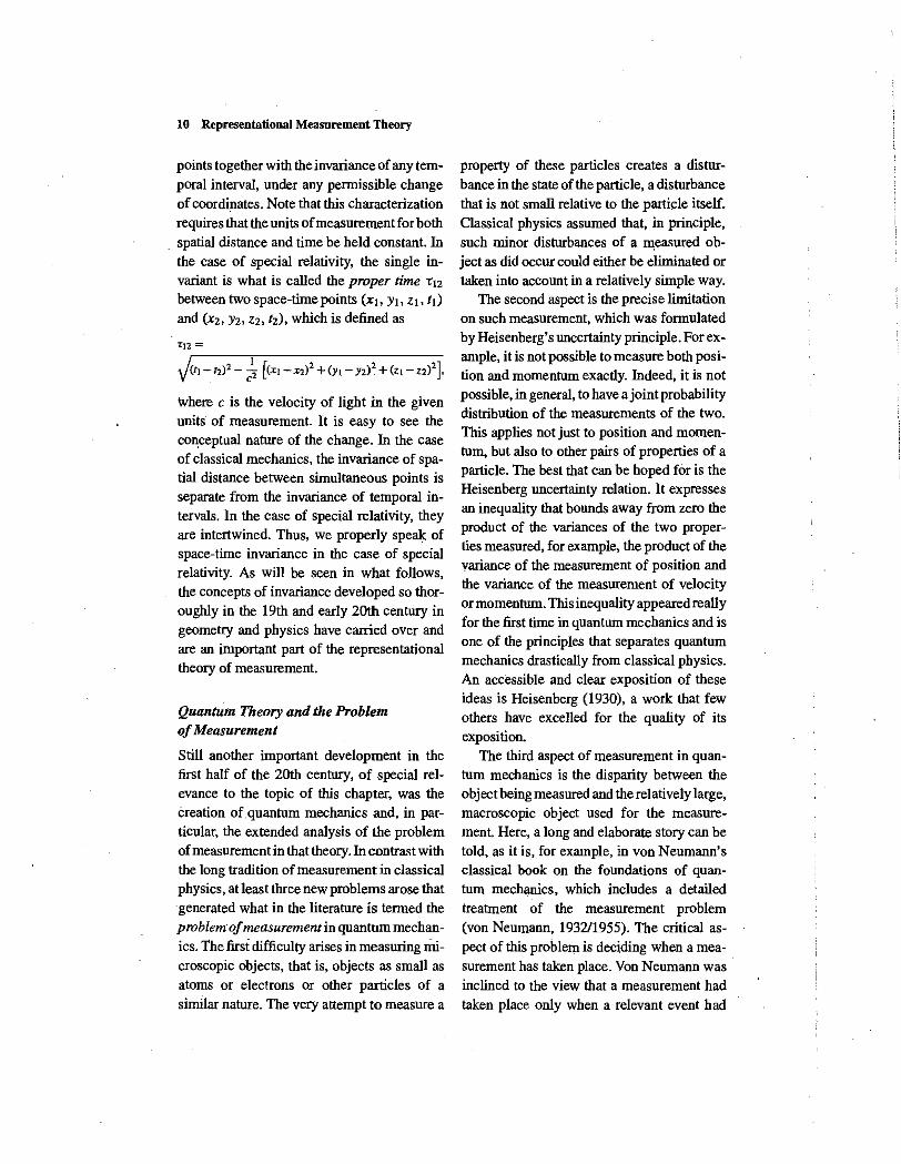
points together with the invariance of any tem­poral interval, under any permissible change of coordinates. Note that this characterization requires that the units of measurement for both spatial distance and time be held constant. In the case of special relativity, the single in­variant is what is called the proper time '12

between two space-time points (x" y" z" tIl and (X2, Y2, Z2, t2), which is defined as

TI2 =

V(tl -: t2)2 - ~ [(XI - X2)2 + (Yt - Y2)2 + (Z\ - Z2)2].

where c is the velocity of light in the given units' of measurement. It is easy to see the conceptual nature of the change. In the case of classical mechanics, the invariance of spa­tial distance between simultaneous points is separate from the invariance of temporal in­tervals. In the case of special relativity, they are intertwined. Thus, we properly speak of space-time invariance in the case of special relativity. As will be seen in what follows, the concepts of invariance developed so thor­oughly in the 19th and early 20th century in geometry and physics have carried over and are an important part of the representational theory of measurement.

QuantUm Theory and the Problem of Measurement

Still another important development in the first half of the 20th century, of special rel­evance to the topic of this chapter, was the creation of quantum mechanics and, in par­ticular, the extended analysis of the problem of measurement in that theory. In contrast with the long tradition of mea::mrement in classical physics, at least three new problems arose that generated what in the literature is termed the problem' of measurement in quantum mechan­ics. The firsi difficulty arises in measuring mi­croscopic objects, that is, objects as small as atoms or electrons or other particles of a similar nature. The very attempt to measure a

property of these particles creates a distur­bance in the state of the particle, a disturbance that is not smalI relative to the particle itself. Classical physics assumed that, in principle, such minor disturbances of a measured ob­ject as did occur could either be eliminated or taken into account in a relatively simple way.

The second aspect is the precise limitation on such measurement, which was formulated by Heisenberg's uncertainty principle. For ex­ample, it is not possible to measure both posi­tion and momentum exactly. Indeed, it is not possible, in general, to have a joint probability distribution of the measurements of the two. This applies not just to position and momen­tum, but also to other pairs of properties of a particle. The best that can be hoped for is the Heisenberg uncertainty relation. It expresses an inequality that bounds away from zero the product of the variances of the two proper­ties measured, for example, the product of the variance of the measurement of position and the variance of the measurement of velocity or momentum. This inequality appearedreally for the first time in quantum mechanics and is one of the principles that separates quantum mechanics drastically from classical physics. An accessible and clear exposition of these ideas is Heisenberg (1930), a work that few others have excelled for the quality of its exposition.

The third aspect of measurement in quan­tum mechanics is the disparity between the object being measured and the relatively large, macroscopic object used for the measure­ment. Here, a long and elaborate story can be told, as it is, for example, in von Neumann's classical book on the foundations of quan­tum mech~cs, which includes a detailed treatment of the measurement problem (von Neumann, 193211955). The critical as­pect of this problem is deciding when a mea- . surement has taken place. Von Neumann was inclined to the view that a measurement had taken place only when a relevant event had

occurred in-'-the consciousness of some ob­server. More moderate subsequent views are satisfied'with the position that an observation takes place when a suitable recording has been made by a calibrated instrument.

Although we shall not discuss further the problem of measurement in quantum mechan­ics, nor even the application of the ideas to measurement in psychology, it is apparent that there is some resonance between the difficul­ties mentioned and the difficulties of measur­ing many psychological properties.

19th- and Early 20th-Century Psychology

Fechner's Psychophysics

Psychology was not a separate discipline until the late 19th century. Its roots were largely in philosophy with significant additions by med­ical and physical scientists. The latter brought a background of successful physical measure­ment, which they sought to re-create in sen­sory psychology at the least. The most promi­nent of these were H. Helmholtz, whose work among other things set the stage for extensive measurement, and G. T. Fechner, whose Elemente der Psychophysik (Elements of Psychophysics; 186011966) set the stage for subsequent developments in psychological measurement. We outline the problem faced in trying to transplant physical measurement and the nature of the proposed solution.

Recall that the main measurement device used in 19th-century physics was concatena­tion: Given two entities that exhibit the at­tribute to be measured, it was essential to find a method of concatenating them to form a third entity also exhibiting the attribute. Then one showed empirically that the structure satisfies the axioms of extensive measurement, as dis­'cussed earlier. When no empirical concatena­tion operation can be found, as for example with density, one could not do fundamental measurement. Rather, one sought an invari­ant property stated in terms of fundamentally

A Brief History of Measurement 11

measured quantities called derived measure­ment. Density is an example.

When dealing with sensory intensity, phys­ical concatenation is available but just recov­ers the physical measure, whi"h does not at all well correspond with subjective judgments such as the half loudness of a tone. A new approach was required. Fechner continued to accept the idea of building up a measure­ment scale by adding small increments, as in the standard sequences of extensive mea­surement, and then counting the number of such increments needed to fill a sensory in­terval. The question was: What are the small equal increments to be added? His idea was that they correspond to 'just noticeable dif­

,ferences" (JND); when one first encounters the idea of a JND it seems to suggest a fixed threshold, but it gradually was interpreted to be defined statistically. To be specific, sup­

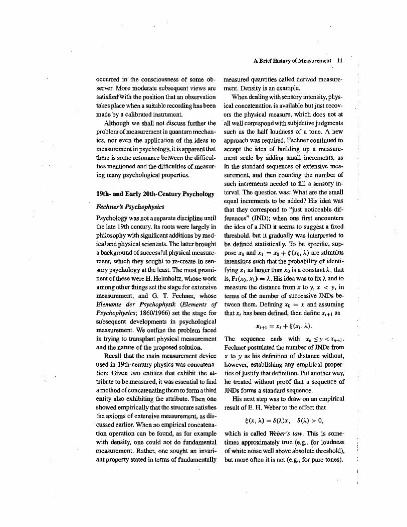
pose Xo and Xl = Xo + Hxo, A) are stimulus intensities such that the probability of identi­fying Xl as larger than Xo is a constant A, that is, Pr(xo, Xl) = A. His idea was to fix A and to measure the distance from X to y, X < y, in terms of the number of successive JNDs be­tween them. Defining Xo = X and assuming that Xi has been defined, then define Xi+l as

Xi+l = Xi + ~(Xi, A).

The sequence ends with xn:::: Y < Xn+l. Fechner postulated the number of JNDs from X to y as his definition of distance without, however, establishing any empirical proper­ties of justify that definition. Put another way, he treated without proof that a seqnence of JNDs forms a standard sequence.

His next step was to draw on an empirical result of E. H. Weber to the effect that

Hx, A) = 8 (A)X , 8(A) > 0,

which is called Weber's law. This is some­times approximately true (e.g., for loudness of white noise well above absolute threshold), but more often it is not (e.g., for pure tones).

12 Representational Measurement Tbeory

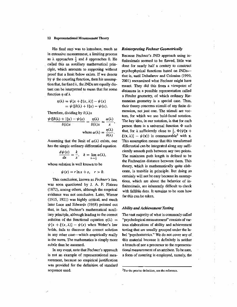
His final step was to introduce, much as in extensive measurement, a limiting process as A approaches 4 and 8 approaches O. He called this an auxiliary mathematical prin­ciple, which amounts to supposing without proof that a limit below exists. If we denote by '" the counting function, then his assump­tion that, for fixed A, the JNDs are equally dis­tant can be interpreted to mean that for some function 11 of A

II(A) = "'Ix + Hx, A)l - "'(x) = "'(18(A) + llx) - "'(x).

Therefore, dividing by 8(A)x

"'(18(A) + Ilx) - "'(x) II(A) a(A) =--=--

8(A)x 8(A)x x

11 (A) where a(A) = 8(A)'

Assuming that the limit of a(A) exists, one has the simple ordinary differential equation

d1fr(x) k =

dx x' k = lim a(A),

).-lo-! whose solution is well known to be

"'(x)=rlnx+s, r>O.

This conclusion, known as Fechner's law, was soon questioned by J. A. F. Plateau (1872), among others, although the emprical evidence was not conclusive. Later, Wiener (1915, 1921) was highly critical, and much later Luce and Edwards (1958) pointed out that, in fact, Fechner's mathematical auxil­iary principle, although leading to the correct solution of the functional equation II(A) = "'Ix + ~(x, A)l - "'(x) when Weber's law holds, fails to discover the correct solution in any other case-which empirically really is the norm. The mathematics is simply more subtle than he assumed.

In any event, note that Fechner's approach is not an example of representational mea­surement, because no empirical justification was provided for the definition of standard sequence used.

Reinterpreting Fechner GeometricaUy

Because Fechner's JND approach using in­finitesimals seemed to be flawed, little was done for nearly half a century to construct psychophysical functions based on JNDs­that is, until Dzhafarov and Colonius (1999, 200 I) reexamined what Fechner might have meant. They did this from a viewpoint of distances in a possible representation called a Finsler geometry, of whicb ordinary Rie­mannian geometry is a special case. Thus, their theory concerns stimuli of any finite di­rnension, not just one. The stimuli are vec­tors, for which we use bold-faced notation. The key idea, in our notation, is that for each person there is a universal function <t> such that, for A snfficiently close to 4, <t>("'lx + ~(x, A)l - ",(x)) is comeasurable3 with x. This assumption means that this transformed differential can be integrated along any suffi­ciently smooth path between any two points. The minimum path length is defined to be the Fechnerian distance between them. This theory, which is mathematically qnite elab­orate, is testable in principle. But doing so certainly wi\l not be easy because its assump­tions, which are about the behavior of in­finitesiMals, are inherently difficult to check with fallible data. It remains to be seen how far this can be taken.

Ability and Achievement Testing

The vast majority of what is commonly called "psychological measurement" consists of var­ious elaborations of ability and achievement testing that are usually grouped under the la· bel "psychometrics." We do not cover any of this material because it definitely is neither a branch of nor a precursor to the representa­tional measurement of an attribute. To be sure, a form of counting is employed, namely, the

JPor the precise definition, see the reference.

items on a test that are correctly answered, and this numberis statistically uormed over a par­ticular age or other feature so that the count is transformed into a normal distribution, Again, no axioms were or are provided. Of the psy­chometric approaches, we speak only of a por­tion ofThurstone's work that is closely related to sensory measurement. Recently, Doignon and Falmagne (1999) have developed an ap­proach to ability measurement, called knowl­edge spaces, that is influenced by representa­tional measurement considerations.

Thurston.'s Discriminal Dispersions

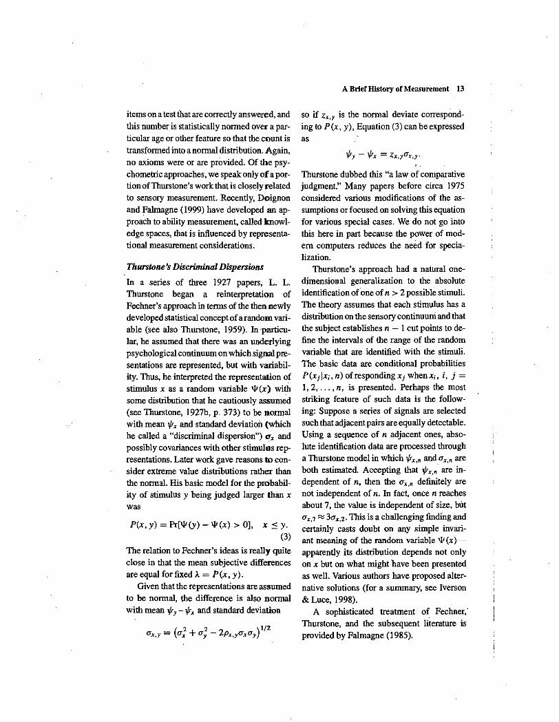
In a series of three 1927 papers, L. L. Thurstone began a reinterpretation of Fechner's approach in terms of the then newly developed statistical concept of arandom vari­able (see also Thurstone, 1959). Inparticu­lar, he assumed that there was an underlying psychological continuum on which signal pre­sentations are represented, but with variabil­ity. Thus, he interpreted the representation of stimulus x as a random variable \jI (x) with some distribution that he cautiously assumed (see Thurstone, 1927b, p. 373) to be normal with mean "'x and standard deviation (which he called a "discrintinal dispersion") fTx and possibly covariances with other stimulus rep­resentations. Later work gave reasons to con· sider extreme value distributions rather than the normal. His basic model for the probabil­ity of stimulus y being judged larger than x was

P(X, y) = Pr(\jI(y) - \jI(x) > 0], x:s y.

(3)

The relation to Fechner's ideas is really quite close in that the mean subjective differences are equal for fixed A = P (x, y).

Given that the representations are assumed to be normal, the difference is also normal

with mean '" y - "'x and standard deviation

A Brief History of Measurement 13

so if Zx,y is the normal deviate correspond­ing to P(x, y), Equation (3) can be expressed

as

"'y - "'x = zx.y"x.y·

Thurstone dubbed this "a law of comparative judgment." Many papers before circa 1975 considered various modifications of the as­sumptions or focused on solving this equation for various special cases. We do not go into this here in part because the power of mod­ern computers reduces the need for specia­lization.

Thurstone's approach had a natural one­dimensional generalization to the absolute identification otone of n > 2 possible stimuli. The theory assumes that each stimulus has a distribution on the sensory continuum and that the subject establishes n - 1 cut points to de­fine the intervals of the range of the random variable that are identified with the stimuli. The basic data are conditional probabilities P(xj!xi,n)ofrespondingxjwhenxi, i, j = 1, 2, ... , n, is presented. Perhaps the most striking feature of such data is the follow­ing: Suppose a series of signals are selected such that adjacent pairs are equally detectable. Using a sequence of n adjacent ones, abso­lute identification data are processed through

a Thurstone model in which "'x.n and "x.n are both estimated. Accepting that "'x,n are in­dependent of n, then the "x.n definitely are not independent of n. In fact, once n reaches about 7, the value is independent of size, but

"x.7 "" 3"x.2. This is a challenging finding and certainly casts doubt on any simple invari­ant meaning of the random variable \jI (x)­

apparently its distribution depends not only on x but on what ntight have been presented as well. Various authors have proposed alter­native solutions (for a summary, see Iverson & Luce, 1998).

A sophisticated treatment of Fechner; Thurstone, and the subsequent literature is provided by Falmagne (1985).

14 Representational Measurement Theory

Theory of Signal Detectability

Perhaps the most important generalization of Thurstone's idea is that of the theory of sig­nal detectability, in which the basic change is to assume that the experimental subject can establish a response criterion P, in general different from 0, so that

P(x, y) = Pr[IjI(y) - ljI(x) > Pl, x:s: y.

Engineers first developed this model. It was adoped and elaborated in various psycho­,logical sources, including Green and Swets (1974) and Macmillan and Creelman (1991), and it- has been widely applied throughout psychology.

Mid-20th-Century Psychological Measurement

Campbell's Objection to Psychowgical Measurement

N. R. Campbell, a physicist turned philoso­pher of physics who was especially concerned with physical measurement, took the very strong position that psychologists, in partic­ular, and social scientists, in general, had not come up with anything deserving the name of measurement and probably never could. He was supported by a number of other British physicists. His argument, though somewhat elaborate, actually boiled down to asserting the truth of three simple propositions:

(i) A prerequisite of measurement is some form of empirical quantification that can be accepted or rejected experimentally.

(ii} The only known form of such quantifi­cation arises from binary operations of concatenation that can be shown empir­ically to satisfy the axioms of extensive measurement.

(iii) And psychology has no such extensive operations of its own.

Some appropriate references are Campbell (192011957,1928) andFergusonet al. (1940).

Stevens's Response

In a prolonged debate conducted before a subcommittee of the British Association for the Advancement of Sciences. the physicists agreed on these propositions and the psychol­ogists did not, at least not fully. They accepted (iii) but in some measure denied (i) and (ii), although, of course, they admitted that both held for physics. The psychophysicist S. S. Stevens became the primary spokesperson for the psychological community. He first formu­lated his views in 1946, but his 1951 chapter in the first version of the Handbook of Exper­imental Psychology, of which he was editor, made his views widely known to the psycho­logical community. They were complex, and at the moment we focns only on the part rele­vant to the issue of whether measurement can be justified outside physics.

Stevens' contention was that Proposition (i) is too narrow a concept of measurement, so (ii) and therefore (iii) are irrelevant. Rather, he argued for the claim that "Measurement is the assignment of numbers to objects or events according to rule .... The rule of assignment can be any consistent rule" (Stevens, 1975, pp. 46-47). The issne was whether the rule was sufficient to lead to one of several scale types that he dubbed nominal, ordinal, inter­val, ratio, and absolute. These are sufficiently well known to psychologists that we need not describe them in much detail. They concern the uniqueness of numerical representations. In the nominal case, of which the assignment of numbers to football players was his exam­ple, any permutation is permitted. This is not generally treated as measurement because no ordering by an attribute is involved. An or­dinal scale is an assignment that can be sub­jected to any strictly increasing transforma­tion, which of course preserves the order and nothing else. It is a representation with infinite

degrees offreedom. An interval scale is one in which there is an arbitrary zero and unit; but

once picked, no degrees of freedom are left. Therefore, the admissible transformation is

l/f >---> rl/f+s, (r > 0). As stated,sucharep­resentation has to be on all of the real numbers. If, as is often the case, especially in physics, one wants to place the representation on the positive real numbers, then the transforma­

tion becomes l/f+ r--+ s'l/f+., (r > 0, s' > 0). Stevens (1959, pp. 31-34) called a represen­tation unique up to power transfonnations a log-interval scale but did not seem to recog­nize that it is merely a different way of writ­ing an interval scale representation l/f in which l/f = In l/f + and s = In s' . Whichever one uses, it has two degrees of freedom. The ratio case is the interval one with r = I. Again, this has two forms depending on the range of l/f. For the case of a representation on the reals, the admissible transformations are the translations l/f r--+ l/f + s. There is a differ­ent version of ratio measurement that is inher­ently on the reals in the sense that it cannot he placed on the positive reals. In this case, o is a true zero that divides the representa­tion into inherently positive and negative por­tions, and the admissible transformations are

l/f r--+ rl/f, r > O. Stevens took the stance that what was im­

portant in measurement was its uniqueness properties and that they could come about in ways different from that of physics. The remaining part of his career, which is sum­marized in Stevens (1975), entailed the de­velopment of new methods of measnrement that can all be encompassed as a form of sen­sory matching. The basic instruction to sub­

jects was to require the match of a stimu­lus in one modality to that in another so that the subjective ratio between a pair of stim­uli in the one dimension is maintained in the subjective ratio of the matched signals. This is called cross-modal matching. When one of the modalities is the real numbers, it is

Representational Approach after 1950 15·

one of two forms of magnitude matching­magnitude estimation when numbers are to be matched to a sensory stimuli and magnitude

production when numbers are the stimuli to be matched by some physical stimuli. Using geo­

metric means over subjects, he found the data to be quite orderly-power functions of the usual physical measures of intensity. Much of this work is covered in Stevens (1975).

His argument that this constituted a form of ratio scale measurement can be viewed in two distinct ways. The least charitable is that of Michell (1999), who treats it as little more than a play on the word "ratio" in the scale type and in the instructions to the subjects. He feels that Stevens failed to understand the need for empirical conditions to justify numerical representations. Narens (1996) took the view that Stevens' idea is worth trying to formal­ize and in the process making it empirically testable. Work along these lines continues, as

discussed later.

REPRESENTATIONAL APPROACH AFTER 1950

Aside from extensive measurement, the repre­sentational theory of measurement is largely a creation by behavioral scientists and math­ematicians during the second half of the 20th century. The basic thrust of this school of thought can be summarized as accept­ing Campbell's conditions (i), quantification based on empirical properties, and (iii), the social sciences do not have concatemi.tion op­erations (although even that was never strictly correct, as is shown later, because of probabil­ity based on a partial operation), and rejecting the claim (ii) that the only form of quantifica­tion is an empirical concatenation operation. This school disagreed with Stevens' broaden­ing of (i) to any rule, bolding with the physi­cists that the rules had to be established on

firm empirical grounds.

16 Representational Measurement Theory

To do this, one had to establish the exis­tence of schemes of empirically based mea­surement tl).at were different from extensive measurement. Examples are provided here. For greater detail, see PM I, II, III, Narens (1985), or for an earlier perspective Pfanzagl (1968).

Several Alternatives to Extensive Measurement

Utility Theory

The first evidence of something different from extensive measurement was the construction by·von Neumann and Morgenstern (1947) of an axiomatization of expected utility theory. Here, the stimuli were gambles of the form (x, p; y) where consequence x occurs with probability p andy with probability 1-p. The basic primitive of the system was a weak pref­erence order!: over the binary gambles. They stated properties that seemed to be at least rational, if not necessarily descriptive; from them one was able to show the existence of a numerical utility function U over the conse­quences and gambles such that for two binary gambles g, h

g!:h # U(g)::: U(h),

.U(g, p; h) = U(g)p + U(h)(l - p).

Note that this is an averaging representation, called expected utility, which is quite distinct from the adding of extensive measurement (see the subsection on averaging).

Actually, their theory has to be viewed as a form of derived measurement in Campbell's sense because the construction of the U func­tion was in terms of the numerical probabil­ities built into the stimuli themselves. That limitation was overcome by Savage (1954), who modeled decision making under uncer­tainty as acts that are treated as an assignment

of consequences to chance states of nature.4

Savage assumed that each act had a finitenum­ber of consequences, but subsequent gener­alizations permitted infinitely many. Without building any numbers into the domain and us­ing assumptions defended by arguments of rationality, he showed that one can construct both a utility function U and a subjective prob­ability function S such that acts are evaluated by calculating the expectation of U with re­spect to the measure S. This representation is called subjective expected utility (SEU). It is a case of fundamental measurement in Campbell's sense. Indirectly, it involved a partial concatenation operation of disjoint unions, which was used to construct a sub­jective probability function.

These developments led to a very ac­tive research program involving psycholo­gists, economists, and statisticians. The basic thrust has been of psychologists devising experiments that cast doubt on either a repre­sentation or some of its axioms, and of theorists of all stripes modifying the theory of accommodate the data. Among the key summary references are Edwards (1992), Fishburn (1970, 1988), Luce (2000), Quiggin (1993), and Wakker (1989).

Difference Measurement

The simplest example of difference measure­ment is location along a line. Here, some point is arbitrarily set to be 0, and other points are defined in terms of distance (length) from it, with those on one side defined to be positive and those on the other side negative. It is clear in this case that location measurement forms an example of interval scale measurement

4Some aspects of Savage's approach were anticipate!1 by Ramsey (1931). but that paper was not widely known to psycholegists and economists. Almost simultane­ously with the appearance of Savage's work, Davidson. McKinsey, and Suppes (1955) drew on Ramsey's ap­proach. and Davidson. Suppes, and Segal (1957) tested it experimentally.

that is readily reduced to length measurement. Indeed, all forms of difference measurement are very closely related to extensive measure­ment, but with the stimuli being pairs of ele­ments (x, y) that define "intervals." Axioms can be given for this fonn of measurement where the stimuli are pairs (x, y) with both x, y in the same set X. The goal is a numerical representation 'I' of the form

(x, y) !: (u, v)

* rp(x) - rp(y) ~ rp(u) - rp(v).

One key axiom that makes clear how a con­. catenation operation arises is that if (x, y)!:

(x', y') and (y, z) !: (y', z'), then (x, z) !: (x', z').

An important modification is called abso­lute difference measurement, in which the goal is changed to

(x, y) !: (u, v)

* Irp(x) - rp(y)1 ~ Irp(u) - rp(v)l·

This form of measurement is a precursor to various ideas of similarity measurement important in multidimensional scaling. Here the behavioral axioms become considerably more complex. Both systems can be found in FM I, Chap. 4.

An important generalization of absolute difference measurement is to stimuli with n factors; it nnderlies developments of geomet­ric measurement based on stimulus proximity. This can be found in FM n, Chap. 14.

Additive Conjoint Measurement

Perhaps the single development that most persuaded psychologists that fundamental measurement really could he different from extensive measurement consisted of two ver­sions of what is called additive coujoint mea­surement. The first, by Debreu (1960), was aimed at showiug economists how indiffer­ence curves could be used to construct car­dinal (interval scale) utility functions. It was,

Representational Approach after 1950 17

therefore, naturally cast in topological terms. The second (and independent) one by Luce and Tukey (1964) was. cast in algebraic terms, which seems more natural to psychologists and has been shown to include. !he topologi­cal approach as a special case. Again, it was an explanation of the conditions under which equal'attribute curves can give rise to mea­surement. Michell (1990) provides a careful treatment aimed at psychologists.

The basic idea is this: Suppose that an at­tribute is affected hy two indepeudent stim­u!us variables. For example, preference for a reward is affected by its size and the delay in receiving it; mass of an object is affected hy both its volume and the (homogeneous) material of which it is composed; loudness of pure tones is affected hy intensity and fre­quency; and so on. Formally, one can think of the two factors as distinct sets A and X, so an entity is of the form (a, x) where a e A and x eX. The ordering attribute is ~ over such entities, that is, over the Cartesian product A x X. Thus, (a,x)!:(b,y) means that (a, x) exhibits more of the attribute in question than does (b, y). Again, the order­ing is assumed to he a weak order: transitive and connected. Monotonicity (called indepen­dence in this literature) is also assumed: For a,beA,x,yeX

(a, x)!: (b, x) * (a, y)!: (b, y).

(a, x)!: (a, y) * (b, x)!: (b, y). (4)

This familiar property is often examined in psychological research in which a dependent variable is plotted against, say, a measure of the first component with the second compo­nent shown as a parameter of the curves. The property holds if and only if the curves do not cross.

It is easy to show that this condition is not sufficient to get an additive representa­tion of the two factors. If it were, then any set" of nouintersecting curves in the plane could be rendered parallel straight lines by suitable

18 Representational Measurement Theory

nonlinear transfonnations of the axes. More is required, namely, the Thomsen condition, which arose in a mathematically closely related area called the theory of webs. Let­ting - denote the indifference relation of ,e, the Thomsen condition states

(a, z) - (c, y)} (c, x) _ (b, z) =} (a, x) - (b, y).

Note that it is a fonn of cancellation--of c in the first factor and z in the second.

These, together with an Archimedean property establishing commensurability and some fonn of density of the factors, are enough to establish the following additive representation: There exist numerical func­tions 1{! A on A and 1{!x on X such that

(a, x),e (b, y)

{} 1{!A(a) + 1{!x(x) 2: 1{!A(b) + 1{!x(Y)·

This representation is on all of the real num­bers. A multiplicative version on the positive real numbers exists by setting ~i = exp 1{!,. The additive representation fonns an inter­val scale in the sense that 1{!~, 1{!~ fonns another equally good representation if and only if there are constants r > 0, SA, Sx such that

1{!~ = r1{!A +SA,

1{!~ = r1{!x + Sx {} ~~ =S~~A' ~~ =s~~~, s; = expsj > O.

Additive conjoint measurement can be generalized to finitely many factors, and it is simpler in the sense that if monotonicily is generalized suitably and if there are at least three factors, then the Thomsen condition can be derived rather than assumed.

Although no concatenation operation is in sight, a family of them can be defined in tenns of -, and they can be shown to satisfy the axioms of extensive measurement. This is the nature of the mathematical proof of the repre­sentation usually given.

Averaging

Some structures with a concatenation opera­tion do not have an additive representation, but rather a weighted averaging representation of thefonn

9'(X 0 y) = 9'(x)w + 9'(y)(1 - w), (5)

where the weight w is fixed. We have already encountered this fonn in the utility system if we think of the gamble (x, p; y) as defining operations op withxopy == (x, p; y),in which case w = w (p). A general theoly of such op­erations was first given by Pfanzagl (1959). It is much like extensive me'asurement but with associativity replaced by bisymmetry: For all stimuli x, y, u, v,

(x 0 y) 0 (u 0 v) ~ (x 0 u) 0 (y 0 v). (6)

It is easy to verify that the weighted-average representation of Equation (5) implies bisym­metry, Equation (6), and x 0 x - x. The eas­iest way to show the converse is to show that defining ,e' over X x X by

(a,x),e'(b,y) {}aox,eboy

yields an additive conjoint structore, from which the result follows rather easily.

Nonadditive Representations

A natoral question is: When does a concatena­tion operation have a numerical representation that is inherently nonadditive? By this, one means a representation for which no sttictly increasing transfonnation renders it additive. Before exploring that, we cite an example of nonadditive representations that can in fact be

transfonned into additive ones. This is helpful in understanding the subtlety of the question.

One example that has arisen in utility the­ory is the representation

U(x Ell y) = U(x)+ U(y) - 8U(x)U(y), (7)

where 8 is a real constant and U is the SEU or rank-dependent utility generalization (see

Luce, 2000, Chap. 4) with an intrinsic zero-­no change from the status quo. Because Equa­tion (7) can be rewritten

1- oU(x $ y) = [I - oU(x)][1 - W(y)],

the transfonnation V = -K In(1 - oU), OK> 0, is additive, that is, vex Ell y) = V (x) + V (y), and order-preserving. The mea­sure V is called a value function. The fonn in Equation (7) is called p-additive because it is the only polynomial with a fixed zero that can be put in additive fonn. The source of this representation is examined in the next major section. It is easy to verify that both the ad­ditive and the nonadditive representations are ratio scales in Stevens' sense. We know from extensive measurement that the change of unit in the additive representation is spme­how reflecting something important about the nnderlying structure. Is that also true of the changes of units in the nonadditive represen­tation? We will return to this point, which can be a source of confusion.

It should be noted that in probability theory for independent events, the p-additive fonn with 0 = I arises since

peA U B) = peA) + PCB) - P(A)P(B).

An earlier, similar example concerning velocity concatenation arose in Einstein's theory of special relativity. Like the psycho­logical one, it entails a representation in the standard measure of velocity that fonns a ratio scale and a nonlinear transfonnation to an additive one that also fonns a ratio scale. We do not detail it here.

Nonadditive Concatenation

What characterizes an inherently nonadditive structure is the failure of the empirical prop­erty of associativity; that is, for some elements x, y, z in the domain.

x 0 (y ° z) 1- (x 0 y) 0 z.

Representational Approach after 1950 19:

Cohen and Narens (1979) made the then­unexpected discovery that if one simply drops associativity from any standard axiomatiza­tion of extensive measurement, not only can one still continue to construct numerical rep­resentations that are onto th~ positive reals but, quite surprisingly, they continue to fonn a ratio scale as well; that is, the representa­tion is unique up to similarity transfonnations. They called this important class of nonaddi­tive representations unit structures. For a full discussion, see Chaps. 19 and 20 of FM III.

A Fundamental Acconnt of Some Derived Measurement

Distribution Laws

The development of additive conjoint mea­surement allows one to give a systematic and fundamental account of what to that point had been treated as derived measurement. For classical physics, a typical situation in which derived measurement arises takes the fonn (A x X,!:;, OA). For example, let A denote a set of volumes and X a set of homogeneous substances; the ordering is that of mass as established by an equal-arm pan balance in a vacuum. The operation 0 A is the simple union of volumes. For this case we know that m = V p, where m is the usual mass measure, V is the usual volume measure, and p is an inferred measure of density.

Observe that (A x X,!:;) forms an addi­tive conjoint structure. By the monotonicity assumption of conjoint measurement; Equa­tion (4), !:; induces the weak order !:;A on A. It is assumed that (A, !:;A, 0A) fonns an ex­tensive structure. Thus we have the extensive representation 'P A of (A,!:;A, 0 A) onto the positive real numbers and a multiplicative conjoint one ~Ah of (A x X,!:;) onto the pos­itive real numbers.

The question is how 'PA and ~A relate. Because both preserve the order !:;A, there

20 Representational Measurement Theory

must be a strictly increasing function F such that ~A = F(rpA). Beyond that, we can say nothing without some assumption describing how the two structures interlock. One that holds for many physical cases, including the motivating mass example, is a qualitative dis­tribution law of the form: For all a, b, c, d in A and x, y in X,

(a, x) ~ (c, y)} (b,x)~(d,y) =>(aoAb,x) ~ (coAd,y).

Using this, one is able to prove that, for some r > 0, s > 0, F(z) = rz'. Because the

. conjoint representation is unique up to power transfonnations, we may select s = I, that is, choose ~A = rp A·

Note that distribution is a substantive, em­pirical property that in each specific case re­quires verification. In fact, it holds for many of the classical physical attributes. From that fact one is able to construct the basic structure of (classical) physical quantities that under­lies the technique called dimensional analysis, which is widely used in physical applications in engineering. It also accounts for the fact that physical units are all expressed as prod­ucts of powers of a relatively small set of units. This is discussed in some detail in Chap. 10 of FM I and in a more satisfactory way in Section 22.7 of FM ITI.

SegregatWn Law

Within the behavioral sciences we have a situation that is somewhat similar to distri­bution. Suppose we return to the gambling structure, where some chance "experiment" is performed, such as drawing a ball from an urn with 100 red and yellow balls of which the respondent knows that the number of red is between 50 and 80. A typical binary gam­bleis of the form (x, C; y), where C denotes a chance event such as drawing a red ball, and the consequence x is received if C occurs and y otherwise, that is, x if a red ball and y if a yellow ball. A weak preference order):; over

gambles is postulated. Letus distinguish gains from losses by supposing that there is a spe­cial consequence, denoted e, that means no change from the status quo. Things preferred to e are called gains, and those not preferred to it are called losses. Assume that for gains (and separately for losses) the axioms leading to a subjective expected utility representation are satisfied. Thus, there is a utility function V over gains and subjective probability function S such that

Vex, C; y) = V(x)S(C) + V(y)[1 - S(C)]

(8)

Vee) = O. (9)

Let 6J denote the operation of receiving two things, called joint receipt. Therefore, g 6J h denotes receiving both of the gambles g and h. Assume that E9 is a commutative5 and mono­tonic operation with e the identity element; that is, for all gambles g perceived as a gain, g 6J e ~ g. Again, some law must link 6J to the gambles. The one proposed by Luce and Fishburn (1991) is segregation: For all gains x, y,

(x, C; e) 6J y ~ (x 6J y, C; y). (10)

Observe that this is highly rational in the sense that both sides yield x 6J y when C occurs and y otherwise, so they should be seen as rep­resenting the same gamble. Moreover, there is some empirical evidence in support of it (Luce, 2000, Chap. 4). Despite its apparent innocence, it is powerful enough to show that V (x 6J y) is given by Equation (7). Thus, in fact, the operation $ fonns an extensive structure with additive representation V = -K In(l- 8V), 8K > O. Clearly, the sign of 8 greatly affects the relation between V and V: it is a negative exponential for 8 > 0, propor­tionalfor 8 = 0, and an exponential for 8 < 0 ..

SLater we examine what happens when we drop this assumption.

Applications of these ideas are given in Luce (2000). Perhaps the most interesting occurs when dealing with x 6) y where x is a gain and y a loss. If we assume that V is additive throughout the entire domain, then with x .':; e .':; y, U (x 6) y) is not additive. This carries through to mixed gambles that no longer have the simple bilinear form of binary SEU, Equation (8).

Invariance and Meaningfulness

Meaningful Statistics

Stevens (1951) raised the following issues in connection with the use of statistics on mea­surements. Some statistical assertions do not seem to make sense in some measurement schemes. Consider a case of ordinal measure­ment in which one set of three observations has ordinal measures 1, 4, and 5, with a mean of 10/3, and another set has measures 2, 3, and 6, with a mean of 11 /3. One would say the former set is, on average, smaller than the second one. But since these are ordinal data, an equally satisfactory representation is 1, 5, and 6 for the first set and 2, 2.1, and 6.1 for the latter, with means respectively 12/3 and 10.2/3, reversing the conclusion. Thus, there is no invariant conclusion about means. Put another way. comparing means is meaning­less in this context. By contrast, the median is invariant under monotonic transformations. It is easy to verify that the mean exhibits suitable invariance in the case of ratio scales.

These observations were immediately chal­lenged and led to what can best be described as a tortured discussion that lasted many years. It was only clarified when the problem was recognized to be a special case of invariance prinCiples that were well developed in both geometry and dimensional analysis.

The main reason why the discussion was confused is that it was conducted at the level of numerical representations, where two kinds of transformations are readily confused, rather

Representational Approach after 1950 21

than in terms of the underlying structure itself. Consider a cubical volume that is 4 yards on a side. An appropriate change of units is from yards to feet, so it is also 12 feet on a side. This is obviously different from the transfor­mation that enlarges each side by ,(factor of3, producing a cube t11ati8 12 yards on a side. At the level of numerical representations, how­ever, these two factor-of-3 changes are all too easily confused. This fact was not recognized when Stevens wrote, but it clearly makes very uncertain just what is meant by saying that a structure has a ratio or other type of repre­sentation and that certain invariances should hold.

Automorphisms

These observations lead one to take a deeper look into questions of uniqueness and invari­ance. Mapping empirical structures ontonu­merical ones is not the most general or funda­mental way to approach invariance. The key to avoiding confusion is to understand what it is about a structure that corresponds to correct admissible transformations of the representa­tion. This turns out to be isomorphisms that map an empirical structure onto itself. Such isomorphisms are called automorphisms by mathematicians and symmetries by physicists. Their importance is easily seen, as follows. Suppose a is an automorphism and f is a ho­momorphism of the structure into a numerical one, then it is not difficult to show that f * a, where * denotes function composition, is an-· other equally good homomorphism into the same numerical structure. In the case of a ra­tio scale, this means that there is a positive nu­merical constant r. such that f * a = r. f . The automorphism captures something about the structure itself, and that is just what is needed.

Consider the utility example, Equation (7), where there are two nonlinearly related rep­resentations, both of which are ratio scales in . Stevens' sense. Thus, calculations of the mean utility are invariant in anyone representation,

22 Representational Measurement Theory

but they certainly are not across representa­tions. Which should be used, if either? It turns out. on careful examination that the one set of transformations corresponds to the auto­morphisms of the underlying extensive struc­ture. The second set of transformations cor­responds to the antomorphisms of the SEU structure, not Ell. Both changes are important, but different. Which one should be used de­pends on the question being asked.

J.nvariance

An important use of automorphisms, first em­phasized for geometry by Klein (187211893) and heavily used by physicists and engineers in the method of dimensional analysis, is the idea that meaningful statements should be invariant under automorphisms. ·Consider a structure with various primitive relations. It is clear that these are invariant under the au­tomorphisms of the structure, and it is natural to suppose that anything· that can be mean­ingfully defined in terms of these primitives should also be invariant. Therefore, in partic­ular, given the structure of physical attributes, any physical law is defined in terms of the at­tributes and thus must be invariant. This def­initely does not mean that something that is invariant is necessarily a physical law. In the case of statistical analyses of measurements, we want the result to exhibit invariance appropriate to the structure underlying the measurements.

To answer Stevens' original question about statistics then entails asking whether the hy­pothesis being tested is meaningful (invariant) when translated back into assertions about the underlying structure. Doing this correctly is sometimes subtle, as is discussed in Chap. 22 of PM m and much more fully by Narens (2001).

Trivial Automorphisms and Invarianc.

Sometimes structures have but one automor­phism, namely the function that maps each

element of the structure into itself-the iden­tity function. For example, in the additive structure of the natural numbers with the stan­dard ordering, the only automorphism is the one that simply matches each number to itself: o to 0, ito I, and so on.

Within the weak ordering;:: of ~ structure, there are trivial automorphisms beyond the identity mapping, namely, those that just map an element a to an equivalent element b; that is, the relation a ~ b holds.

Consider invariance in such structures. We quickly see that the approach cannot yield any significant results because everything is in­variant. This remark applies to all finite struc­tures that are provided with a weak ordering. Thus, the only possibility is to examine the invariant properties of the structure of the set of numerical representations.

Let a finite empirical structure be given with a homomorphism I mapping the struc­ture into a numerical structure. We have al­ready introduced the concept of an admissi­blenumerical transformation rp of I, namely, a one-one transformation of the range of I onto a possibly different set of real numbers, such that rp * I is a homomorphism of the em­pirical structure. In order to fix the scale type and thus the nature of the invariance of the empirical structure, we investigate the set of all such homomorphisms for a given empirical structure. In the case of weight, any two homo­morphisms 11 and h are related by a positive similarity transformation; that is, there is a positive real number r > 0 such that r 11 = h. In the qualitative probability case with inde­pendence, r = I, so the set of all homomor­phisms has only one element. With r =f 1 in the general similarity case, invariance is then characterized with respect to the mUltiplica­tive group of positive real numbers, each num­ber in the group constituting a change of unit. A numerical statement about a set of numer­ical quantities is then invariant if and only if its truth value is constant under any changes of

unit of any of the quantities. This definition is easily generalized to other groups of numeri­cal transformations such as linear transforma­tions for interval scales.

In contrast, consider a finite difference structure with a numerical representation as characterized earlier. In general, the set of all homomOlphisms from the given finite struc­ture to numerical representations has no natu­ral and simple mathematical characterization. For this reason, much of the general theory of representational measurement is concerned with empirical structures that map onto the full domain of real numbers. It remains true, however, that special finite empirical struc­tures remain important in practice in setting up standard measurement procedures using well-defined units.

Covariant.

In practice, physicists hold on to invariance by introducing and using the concept of co­variants. Typical examples of such covari­ants are velocity and acceleration, neither of which is invariant from one coordinate frame to another under either Galilean or Lorentzian transfonnations, because, among other things, the direction of the velocity or acceleration vector of a particle will in general change from one frame to another. (The scalar magnitude of acceleration is invariant.)

The laws of physics are written in terms of such covariants. The fundamental idea is conveyed by the following. Let Q" ... , Qn be quantities that are functions of the space­time coordinates, with some QiS possibly be­ing derivatives of others, for example. Then, in general, as we go from one coordinate system to another (note that' does not mean deriva­tive) Q" ... , Q~ will be covariant, rather than invariant, so their mathematical form is dif­ferent in the new coordinate system. But any physical law involving them, say,

F(Q" ... , Qn) = 0, (11)

Representational Approach after 1950 23

must have the same form

F(Q;, ... , Q~) = 0

in the new coordinate frame. This same fonn is the important invariant requir~ment.

A simple example from classical mechan­ics is the conservation of momentum of two particles before and after a collision. Let Vi

denote the velocity before and withe velocity after the collision, and m i the mass, i = 1, 2, of each particle. Then the law, in the form of Equation (II), looks like this:

VIm, + V2m2 - (w,m, + W2m2) = 0,

and its transformed form will be, of course,

. V~~l + v;m2 - (w~ml + w~m2) = 0,

but the forms of Vi and Wi will be, in general, covariant rather than invariant.

An Account of Stevens' Scale-Type Classification

Narens (198Ia, 1981b) raised and partially answered the question of why the Stevens' classification into ratio, interval, and ordinal scales makes as much sense as it seems to. His result was generalized by Alper (1987), as described later. The question may be cast as follows: These familiar scale types have, respectively, one, two, and infinitely many de­grees of freedom in the representation; are there not any ~)hers, such as ones having three or 10 degrees of freedom? To a first ap­proximation, the answer is "no," but the pre­cise answer is somewhat more complex than that.

To arrive at a suitable formulation, a spe­cial case may be suggestive. Consider a struc­ture that has representations onto the reals­continuous representations-that form an in­terval scale. Then the representation has the following two properties. First, given num-' bers x < y and u < v, there is a positive affine transformation that takes the pair (x, y) into

24 Representational Measurement Theory

(u, v). It is found by setting u = rx + s, v = ry +s, whencer = ;=; ands =,y;=~v. Thus, in tenns of automorphisms we have the property that there exists one that maps any ordered pair of the structure into any other or­dered pair. This is called two-point homogene­ity. Equally well, if two affine transforma­tions map a pair into the same pair, then they are identical. This follows from the fact that two equations uniquely detennine r and s. In terms of automorphisms, this is called 2-point uniqueness. The latter can be recast by say­ing that any automorphism having two fixed points must be the identity antomorphism.

.In like manner, the ratio scale case is I-point homogeneous and I-pointunique. The generalizations of these concepts to M -point homogeneity and N -point uniqueness are obvious. Moreover, in the continuous case it is easy to show that M :s N. The question ad­dressed by N arens was: Given that the struc­ture is at least I-point homogeneous and N­point unique for some finite N, what are the possibilities for (M, N)? Assuming M = N and a continuous structure, he showed that the only possibilities are (I, I) and (2, 2), that is, the ratio and interval scales. Alper (1987) dropped the condition that M = N and showed that (1,2) can also occur, but that is the only added possibility. In terms of numerical representations on all of the real numbers, the (I, 2) transformations are of the form x r--> r x + s where s is any real and r is in some p:roper, nontrivial subgroup of the multiplicative, positive real g,,;mp. One example is when r is of the form kn ,

where k > 0 is fixed and n ranges over the positive and negative integers.

This result makes clear two things. First, we see that there can be no continuous scales between interval and ordinal, which of course is not finitely unique. Second, there are scales between ratio and interval. None of these has yet played a role in actual scientific measurement. Thus, for continuous structures

Stevens' classification was almost complete, but not quite.

The resnlt also raises some questions. First, how critical is the continuum assumption? The answer is "very": Cameron (1989) showed that nothing remotely like'the Alper­Narens result holds for representations on the rational numbers. Second, what can be said about nonhomogeneous structures? Alper (1987) classified the M = 0 case, but the re­sults are quite complex and apparently not tertibly useful. Luce (1992) explored empir­ically important cases in which homogeneity fails very selectively. It does whenever there are singular points, which are defined to be points of the structure that remain fixed under all automorphisms. Familiar examples are 0 in the nonnegative, mUltiplicative real num­bers and infinity if, as in relativistic velocity, it is adjoined to the system. For a broad class of systems, he showed that if a system has finitely many singUlar points and is homoge­neous between adjacent ones, then there are at most three singular points-a ntinimum, an interior, and a maximum one. The detailed nature of these fixed points is somewhat com­plicated and is not discussed here. One spe­cific utility structure with an interior singular point-an inherent zero-is explored in depth in Luce (2000).

Models of Stevens' Magnitnde Methods

Stevens' (1975) empirical findings, which were known in the 1950s, were a challenge to measurement theorists. What underlies the network of (approximate) power function relations among subjective measures? Luce (1959) attempted to argue in terms of repre­sentations that if, for example, two attributes are eacp' continuous ratio scales,6 with typi­cal physical representations '1'1 and '1'2, then

6Scale types other than ratio were also studied by Luce and subsequent authors.

a matching relation M between them should exhibit an invariance involving an admissi­ble ratio-scale change of the one attribute corresponding under the match to a ratio­scale change of the other attribute, that is, M[rl',(x)] = a(r)<P2(x). From this it is not difficult to prove that M is a power func­tion of its argument. A major problem with this argument is its failure to distinguish two types of ratio scale transformations-changes of unit. such as centimeters to meters-and changes of scale, such as increasing the linear dimensions of a volume by a factor of three. Rozeboom (1962) was very critical of this fail­ure. Luce (1990) reexamined the issue from the perspective of automorphisms. Suppose M is an empirical matching relation between two measurement structures, and suppose that for each translation (i.e., an automorphism with no fixed point) T of the first structure there corresponds to a translation crr of the sec­ond structure such that for any stimulus x of the first structure and any s of the second, then xMs holds if and ouly if for each auto­morphism T oflbe first structure T(x)Mcr,(s)

also holds. This assumption, called transla­tion consistency, is an empirically testable property, not a mere change of units. Assum­ing that the two structures have ratio scale representations, this property is equivalent to a power function relation between the repre­sentations.

Based on some ideas of R. N. Shep­ard, circulated privately and later modified and published in 1981, Krantz (1972) devel­oped a theory that is based on three prim­itives: magnitude estimates, ratio estimates, and cross-modal matches. Various fairly sim­ple, testable axioms were assumed that one would expect to hold if the psychophysical functions were power functions of the cor­responding physical intensity and the ratios of the instructions were treated as mathe­matical ratios. These postulates were shown to yield the expected power function repre-

Representational Approach after 1950 25

sentations except for an arbitrary increasing function. This unknown function was elimi­nated by assuming, without a strong rationale, that the judgments for one continuum, such as length judgments, are veridical, thereby forcing the function to be a' simple multi­plicative factor. This model is summarized in Falmague (1985, pp. 309-313). A somewhat related approach was offered by Fahnagne and Narens (1983), also srmunarized in Palmague (1985, pp. 329-339). It is based not on beha­vioral axioms, but on two invariance- princi­ples that they call meaningfulness and dimen­sional invariance. Like the Krantz theory, it too leads to the form G(I'? 1';') , where G is unspecified beyond being strictly increasing.

Perhaps the deepest published analysis of the problem so far is Narens (1996). Uulike Stevens, he carefully distinguished numbers from numerals, noting that the experimen­tal structure ip.volved numerals whereas the scientists' representations of the phenomena involved numbers. He took seriously the idea that internally people are carrying out the ratio-preservation calculations embodied in Stevens' instructions. The upshot of Narens' axioms, which he carefully partitioned into those that are physical, those that are behav­ioral, and those that link the physical and the behavioral, was to derive two empirical pre­dictions from the theory. Let (x, p, y) mean that the experimenter presents stimulus x and the numeral p to which the subject produces stimulus y as holding the p relation to x. So if 2 is given, then y is whatever the subject feels is twice x. The results are, first, a conunutativ­ity property: Suppose that the subject yield. (x, p, y) and (y, q, z) when done in that order and (x, q, u) and (u, p, v) when the numerals are given in the opposite order. The prediction is z = v. A second result is a multiplicative one: Suppose (x, pq, w), then the prediction is W = z. It is clear that the latter property im­plies the former, but not conversely. Empirical data reported by Ellemeirer and Faulhanuner

26 Representational Measurement Theory

(2000) sustain the fonner prediction and un­

ambiguously reject the latter. Luce (2001) provides a variant axiomatic

theory, based on a modification of some math­ematical results summarized in Luce (20oo) for utility theory. The axioms are fonnulated in tenns of three primitives: a sensory order­ing i:; over physical stimuli varying in inten­sity, the joint presentation x Ell y of signals x and y (e.g., the presentation of pure tones of the same frequency and phase to the two ears), and for &ignals x > y and positive number p

denote by z = (x, p, y) the signal that the sub­ject judges makes interval [y, z] stand in pro­portion p to interval [y, x]. The axioms, such as segregation, Equation (IO), are behavioral and stmctural, and they are sufficient to ensure the existence of a continuous psychophysical measure 'fr from stimuli to the positive real numbers and a continuous function W from the positive reals onto the positive reals and a

constant 8 > 0 such that for Ell commutative

xi:;y * 'fr{x) ~ 'frey), (12)

'fr{x Ell y) = 'fr{x) + 'frey) + 8'fr{x)'fr{y)

(8 > 0), (13)

'fr{x, p, y) - 'frey) = W{p)['frex) - 'frey)].

(14)

We have written Eqnation (14) in this fashion rather than in a fonn comparable to the SEU equation for two reasons: It corresponds to the instructions given the respundents, and W (p) is not restricted to [0, 1]. Recent, cur­rently unpublished, psychophysical data of R. Steingrimsson showed an important case of $

(two-ear loudness summation) that is rarely, if ever, commutative_ This finding motivated Aczel, Luce, and Ng (2001) to explore the

noncommutative, nonassociative cases on the assumpiion Ell has a unit representation (men­tioned earlier) and assuming Equations (12)

and (14) and that certain·unknown functions are differentiable. To everyone's surprise, the only new representations replacing (13) are

either

'fr{x Ell y) = a'fr{x) + 'frey), (a> I)

when x Ell 0>- 0 Ell x, or

'fr{x Ell y) = 'fr{x) + a''fr{y), (a' > I)

when x Ell 0 -<0 Ell x. These are called left- and right-weighted additive fonns, respectively. These representations imply that some fixed dB correction can compensate the nOnCOID­mutativity. Empirical studies evaluating this are underway.

One invariance condition limits the fonn of 'fr to the exponential of a power function of de­viations from absolute threshold, and another one limits the form of W to two parameters for p ~ I and two more for p < I.

The theory not only is able to accommo­date the Ellemeirer and Faulharnmer data but also predicts that the psychophysical function is a power function when E9 is not commuta­tive and only approximately a power function for Ell commutative. Over eight or more or­ders of magnitude, it is extremely close to a power function except near threshold and for very intense signals. Despite its not being a pure power function, the predictions for cross­modal matches are pure power functions.

Errors and Thresholds

To describe the general sources of errors and why they are inevitable in scientific work, we can do no better than quote the opening pas­sage in Gauss's famous work on the theory of least squares, which is from the first part

presented to the Royal Society of Gottingen

in 1821:

However much care is taken with observations of the magnitude of physical quantities, they are necessarily subject to more or less considerable errors. These errors, in the majority of cases, are not simple, but arise simultaneously from several distinct sources which it is convenient to distinguish into two classes.

Certain causes of errors ~epend, for each ob­servation, on circumstances which are variable and independent of the result which one obtains: the errors arising from such sources are called irregular or random, and like the circumstances which produce them, their value is not suscep­tible of calculation. Such are the errors which arise from the imperfection of our senses and all those which are due to irregular exterior causes, such as, for example, the vibrations of the air which make vision less clear; some of the errors due to the inevitable imperfection of the best in­struments belong to the same category. We may mention, for example, the roughness of the in­side of a level, the lack of absolute rigidity, etc.

On the other hand, there exist causes which in all observations of the same nature produce an identical error, or depend on circumstances essentially connected with the result of the ob­servation. We shall call the errof§ of this cate­gory constant or regular.

It is evident that this distinctio'n is relative up to a certain point and- depends on how broad a sense one wishes to attach to the idea of obser­vations of the same nature. For instance, if one repeats indefinitely the measurement of a sin­gle angle, the errors arising from an imperfect division of the circular scale will belong to the class of constant errors. If, on the other hand, one measures successively -several different an­gles, the errors due to the imperfection of the division will be regarded as random as long as one has not formed the table of errors pertaining to each division. (Gauss, 182111957, pp. 1-2)

Although Gauss had in mind problems of errors in physical measurement, it is quite obvious that his conceptual remarks apply as well to psychological measurement and, in fact, in the second paragraph refer directly to the "imperfection of our senses." It was really only in the 19th century that, even in physics, systematic and sustained attention was paid to quantitative problems of errors. For a historical overview of the work pre­ceding Gauss, see Todhunter (1865/1949). As can be seen from the references in the section on 19th- and early 20th-century psychology,

Representational Approach after 1950 27

quantitative atteution to errors in psycholog­ical measurement began at least with Fech­ner in the second half of the 19th century. Also, as already noted, the analysis of thresh­olds in probabilistic tenus really began in psy­Chology with the cited work ,of Thurstone. However, the quantitative and mathematical theory of thresholds was discussed earlier by Norbert Wiener,(1915, 1921). Wiener's treatment was, however, purely algebraic, whereas in tenus of providing relatively di­rect methods of application, Thurstone's approach was entirely probabilistic in char­acter. Already, Wiener (1915) stated very clearly and explicitly how to deal with the fact that with thresholds in perception, the relation of indistinguishability-whether we are talking about brightness of light, loud­ness of sound, or something similar-is not transitive.

The detailed theory was then given in the 1921 paper for constructing a measure up to an interval scale for such sensation-intensities. This is, without doubt, the first time that these important psychological matters were dealt with iu rigorous detail from the standpoint of passing from qualitative judgments to a mea­surement reptesentation. Here is the passage with which Wiener ends the 1921 paper:

In -conclusion, let us consider what bearing all this work of ours can have on experimental psy­chOlogy. One of the great defects under which the latter science atpresent labours is its propen:... sity to try to answer questions without first try- .

ing to find-out just what they ask. The experi­mental investigation of Weber's law7 is a case in point: what most experimenters do take for granted before they begin their experiments is infinitely more important and interesting than any results to which their experiments lead. One of these unconscious assumptions is that sensa­tions or sensation-intervals can be measured,

7Wienermeans what"is now called Fechner's logarithmic law.

28 Representational Measurement Theory

and that this process of measurement can be carried out in one way only. As a result, each new experimenter would seem to have devoted his whole energies to the invention of a method of procedure logically irrelevant to everything that had gone before: one man asks his sub­ject to state when two intervals between sensa­tions of a given kind appear different; another bases his whole work on an experiment where the observer's only problem is to divide a given colour-interval into two equal parts, and so on indefinitely, while even where the experiments are exactly alike, no two people choose quite the same method for working up their results.

. Now, if we make a large number of comparisons of sensation-intervals of a given sort with refer­ence merely to whether one seems larger than another, the methods of measurement given in this paper indicate perfectly unambiguous ways of working up the results so as to obtain some quantitative' law such as that of Weber without introducing such bits of mathematical stupid­ity as treating a '~ust noticeable difference" as an "infinitesimal:' and have the further merit of always indicating some tangible mathematical conclusion, no matter what the outcome of the comparisons may be. (pp. 204-205)

The later and much more empirical work of Thurstone, already referred to, did not, how­ever, give a representational theory of mea­surement as Wiener, in fact, in his own way did.

The work over the last few decades on er­rors and thresholds from the standpoint of rep­resentation theory of measurement naturally falls into two parts. The first part is the al­gebraic theory, and the second is the proba­bilistic theory. We first survey the algebraic results.

Algebraic Theory of Thresholds

The work following Wiener on algebraic thresholds was only revived in the 1950s and. may be found in Goodman (1951), Halphen (1955), Luce (1956), and Scott and Suppes (1958). The subsequent literature is reviewed

in some detail in FM n, Chap. 16. We fol­low the exposition of the algebraic ordinal theory there. We restrict ourselves here to fi­rtite serniorders, the concept first introduced axiomatically by Luce and in 'a modified axiomatization by Scott and Suppes.

Let A be a nonempty set, and let >- be a binary irrefiexive relation on A. Then, (A >-) is a semiorder if for every a, b, c, and d in A

(i) If a >- c and b >- d, then either a >- d or

b>- c. (ii) If a >- band b >- c, then either a >- d or

d >- c.

For finite serniorders (A, >-) we can prove the following numerical representational theorem with constant threshold, which in the present case we will fix at I, so the theorem asserts that there is a mapping f of A into the positive real numbers such that for any a and b in A,

a >- b iff f(a) > feb) + I. A wealth of more detailed and more delicate results on serniorders is to be found in Sec­tion 2 of Chap. 16 of PM n, and research continues on semiorders and various gener­alizations of them, such as interval orders.

Axioms extending the ordinal theory of semiorders to the kind of thing analyzed by Wiener (1921) are in Gerlach (1957); unfor­tunately, to obtaiu a full interval-scale repre­sentation with thresholds involves very com­plicated axioms. This is true to a lesser extent of the axioms for serniordered qualitative probability structures given in Section 16.6.3 of PM n. The axioms are complicated when stated strictly in terms of the relation >- of semiorders.

Probabilistic Theory of Thresholds

For applications in experimental work, it is certainly the case that the probabilistic the­ory of thresholds is more natural and easier to apply. From various directions, there are ex­tensive developments in this area, many but

not all of which are presented in FM II and m. We discuss here results that are simple to formulate and relevant to various kinds of ex­perimenta� work. We begin with the ordinal theory.

A real-valued functionPon A x A is called a binary probability function if it satisfies both

P(a, b) 2: 0,

P(a, b) + P(b, a) = 1.

The intended interpretation of P (a, b) is as the probability of a being chosen over b. We use the probability measure P to define two natural binary relations.

1 aWb iff P(a, b) 2: 2' aSb iff P(a, c) 2: P(b, c), for all c.

In the spirit of semiorders we now define how the relations W and S are related to vari­DUS versions of what is called stochastic tran­sitivity, where stochastic means that the in­dividual instances may not be transitive, but the probabilities are in some sense transitive. Here are the definitions. Let P be a binary probability function on A x A. We define the following for all a, b, c, dinA;

Weak stochastic transitivity: If P(a, b) 2: ! and P(b, c) 2: !, then P(a, c) 2: !.

Weak independence: If P(a, c) > P(b, c), then P(a, d) 2: P(b, d).

Strong stochastic transitivity: If P(a, b) 2: ! and P(b, c) 2:!, then P(a, c) 2: max[P(a, b), P(b, c)].

The basic results for these concepts are taken from Block and Marschak (1960) and Fishburn (1973). Let P be a binary probabil­ity function on A x A, and let W and S be defined as in the previous equations. Then

1- Weak stochastic transitivity holds if W is transitive.

2. Weak independence holds if S is con­nected.

Representational Approach after 1950 29

3. Strong stochastic transitivity holds if W = S. Therefore strong stochastic transi­tivity implies we3k independence; the two

are equivalent if P(a, b) =P ~ for a =P b.

Random Variable Representations

We turn next to random variable representa­

tions for measurement. In the first type, an essentially deterministic theory of measnre­ment (e.g., additive conjoint measurement) is assumed in the. background. But it is recog­nized tbat, for various reasons, variability in response occurs even in what are apparently'

constant circumstances. We describe here the approach developed and used by Falmagne (1976, 1985). Consider the conjoint indiffer­ence (a, p) - (b, q) with a, p, and q given and b to be determined so that the indiffer­ence holds. Suppose that, in fact, b is a random variable which we may denote B(a, p; q). We suppose that such random variables are in­dependently distributed. Since realizations of the random variables occnr in repeated tri­als of a given experiment, we can define the equivalents we started with as holding when the value b is the Pth percentile of the dis­tribution of the random variable B(a, p; q). Falmagne's proposal was to use the median,

P = ~, arid he proceeded as follows. Let "', and ¢>2 be two numerical representations for the conjoint measurement in the usual deter­ministic sense. If we suppose that such an ad­

ditive representation is approximately correct but has an additive error, then we have the following representation;

'I',[B(a, p; q)] = 'I',(a) + 'I'2(q)

- cpz(p) + E(a, p; q),

where the ES are random vanables. It is ob­vious enough how tltis equation provides a natural approximation of standard conjoint measnrement. If we strengthen the assump­tions a bit, we get "an even more natur~l the-' ory by assuming that the random variable

30 Representational Measurement Theory

da, p; q) has its median equal to zero. Using this stronger assumption about all the errors being distributed with a median of zero, Palmagne summarizes assumptions that must be made to have a measurement structure.

Let A and P be two intervals of real num­bers, andletU = (Upq(a) I p, q E P, a E Al

be a collection of random variables, each with a uniquely defined median. Then U is a struc­ture for random additive conjoint measure~ ment if for all p, q, r in P and a in A, the medians m pq (a) satisfy the following axioms:

(i) They are continuous in all variables p, q, anda.

(il) They are strictly increasing in a and p, and strictly decreasing in q.

(iii) They map A into A.

(iv) They satisfy the cancellation rule with respect to function composition *. i.e ..

(mpq * mq,)(a) = mp'(a),

whenever both sides are defined.

Por such random additive conjoint mea­surement strnctnres, Pahnagne (1985, p. 273) proved that there exist real-valued continuous strictly increasing functions <1>, and ",,-, de­fined on A and P respectively, such that for anyJJpq(a) inU,

\?'[Upq{a)]

= '!'2(p) + \?z(q) - 1", (a) + <pq(a),

where <pq(a) is a random variable with a unique median equal to zero. Moreover, if 1"; and 1"2 are two other such functions, then

and

\?2(P) = OI\?Z(p) + Y,

where 01 > O. Statistical tests of these ideas are not a

simple matter but have been studied in or­der to make the applications practical. Major

references are Palmagne (1978); Pahnagne and Iverson (1979); Palmagne, Iverson, and Marcovici (1979); and Iverson and Palmagne (1985). Recent important work on probabil­ity models includes Doignon and Regenwetter (1997); Palmagne and Regenwetter (1996); Palmagne, Regenwetter, and Grofman (1997); Marley (1993); Niederee and Heyer (1997); Regenwetter (1997); and Regenwetter and Marley (in press).

Qualitative Moments

Another approach to measuring, in a repre­sentational sense, the distribution of a random variable for given psychological phenomena is to assume that we have a qualitative method for measuring the moments of the distribution of the random variable. The experimental pro­cedures for measuring such raw moments will vary drastically from one domain of experi­mentation to another. Theoretically, we need only to assume that we can judge qualita­tive relations of one moment relative to an­other and that we have a standard weak order­ing of these qualitatively measured moments. The full formal discnssion of these matters is rather intricate. The details can be found in Section 16.8 ofFM II.

Qualitative Density Functions

As is familiar in all sorts of elementary prob­ability examples, when a distribution has a given fonn, it is often much easier to char­acterize it by a density distribution of a ran­dom variable than by a probability measure on events or by the method of moments as jnst mentioned. In the discrete case, the situation is formally quite simple. Each atom (Le., each atomic event) in the discrete den­sity has a qualitative probability, and we need­judge only relations between these qualitative probabilities. We require of a representing dis­crete density function p on {a" ... ,anI the

following three properties:

(i) p(a,) 2: O.

(ii) L:7=1 peal) = 1.

(iii) peal) 2: p(aj) iff a, !:aj.

Note that the aj are not objects or stimuli in an experiment, but qualitative atomic events, exhaustive and mutually exclusive. Also note that in this discrete case it follows that p(a,):5 I, whereas in the continuous case this is not true of densities.

We also need conditional discrete densi­ties. For this purpose we assume that the

. underlyiug probability space X is linite or de­numerable, with probability measures P on the given fantily F of events. The relation of the density p to the measure P is, for a, an atom of X,

peal) = petal})

Then if A is any event such that peA) > 0,

peal I A) = P({a;} I A),

and, of course, peal I A) is now a discrete den­sity itself, satisfying (i) through (iii).

Here are two simple, but useful, examples of this approach. Let X be a finite set. Then the uniform density on X is characterized by all atoms being equivalent in the qualitative ordering .t. that is,

ai ""J aj.

We may then easily show that the unique den­sity satisfying the equivalence and (i), (ii), and (iii) is

1 peal) =-,

n

where n is the number of atoms iu X. Among the many possible discrete distri­

butions, we consider just one further exam­ple, which has application in experiments in which the model being tested assumes a prob­

ability of change of state iudependent of the time spent in the current state. In the case of discrete trials, such a memoryless process has

Representational Approach after 1950 31

a geometric distribution that can be tested or derived from some simple properties of the discrete but denumerable set of atomic events

(aI, ... ,a" ... J, on each of which is a posi­tive qualitative probability of the occilrrence of the change of state. The numbering of the atoms intuitively corresponds to the trials of an experiment. The atoms are ordered in qual­itative probability by the relation!:. We also introduce a restricted conditional probability. If i > j then a, I A j is the conditional event that the change of state will occur on trial i given that it has not occurred on or before trial j. (Note thathere A j means no change of state from trial 1 through j.) The qualita­tive probability ordering relation is extended to include these special conditional events as well.

The two postulated properties, in addition to (i), (ii), and (iii) given above, are these:

(iv) Order property: a, !: a j iff j 2: i;

(v) Memoryless property: a'+I I A, ~. al·

It is easy to prove that (iv) implies a weak ordering of!:. We can then prove that p(a.) has the form

p(a.) = e(l - e)"-I (0 < c < 1).

Properties (i) through (v) are satislied, but they are also satisfied by any other e', 0 < e' < 1. For experiments testing only the memoryless property, no estimation of e is required. If it is desired to estimate e, the standard estimate is the sample mean m of the trial numbers on which the change of state was observed, since themeanJLofthedensity p(a.) = e(l-e)·-1 satisfies the following equation:

1-e JL= --.

e

For a formal characterization of the full

qualitative probability for the algebra of events-fiot just atoinic events-in the case of the geometric distributiou, see Suppes (1987). For the closely related but mathematically

32 Representational Measurement Theory

more complicated continuous analogue (Le., the ellponential distribution), see Suck (1998).

GENERAL FEATURES 0)<' THE AXIOMATIC APPROACH

Background

History

The story of the axiomatic method begins with the ancient Greeks, probably in the fifth cen­tury B.C. The evidence seems pretty convinc­ing that it developed in response to the early crisis in the foundations of geometry men­tioned earlier, namely, the problem of incom­mensurable magnitudes. It is surprising and important that the axiomatic method as we think of it was largely crystallized in Euclid's Elements, whose author flourished and taugbt in Alexandria around 300 B.C. From a mod­ern standpoint, Euclid's schematic approach is flawed, but compared to any other standard to be found anywhere else for over two mil­lennia, it is a remarkable achievement. The next great phase of axiomatic development occurred, as already mentioned, in the 19th century in connection with the crisis gener­ated in the foundations of geometry itself. The third phase was the fonnalization within logic of the entire language used and the realization that results that could not be proved otherwise can be achieved by such complete logical for­malization. In view of the historical review presented earlier in this article, we will con­centrate on only this third phase in this section.

What Comes before the Axioms

Three main ingredients need to be fixed in an 'axiomatization before the axioms are for­mulated. First, there must be agreement on the general framework used Is it going to be an infonnal, set-theoretical framework or one fonnalized within logic? These two al­ternatives are analyzed in more detail later.

The second ingredient is to fix the primi­tive concepts of the theory being axioma­tized. For example, in almost all theories of choice we need an ordering relation as a prim­itive concept, which means, fonnally, a binary relation. We also often need, ~s mentioned earlier, a binary operation as, for example, in the cases of extensive measurement and averaging. In any case, whatever the prim­itives may be, they should be stated at the beginning. The third ingredient, at least as important, is clarity and explicitness about what other theories are being assumed. It is a characteristic feature of empirical axiomatiza­tions that some additional mathematics is usu­ally assumed, often without explicit notice. This is not true, however, of many qUalita­tive axiomatizations of representational mea­surement and often is not true in the founda­tions of geometry. In contrast, many varieties of probabilistic modeling in psychology do assume some prior mathematics in fonnulat­ing the axioms. A simple example of this was Falmagne's axioms for random addi­tive conjoint measurement, presented earlier . . There, such statistical notions as the median and such elementary mathematical notions as that of continuity were assumed without further explanation or definition.

Another ingredient, less important from a fonnal standpoint bot of considerable impor­tance in practice, are the questions of whether notions defined in tenns of the primitive cou­cepts should be introduced when fonnulating the axioms and whether auxiliary mathemati­cal notions are assumed in stating the axioms. The contrasting alternative is to state the ax­ioms strictly in terms of the primitive notions. From the standpoint oflogical purity, the lat­ter course seems desirable, but in actual fact it is often awkward and intuitively unappealing to state all of the axioms in terms of the prim­itive concepts only. A completely elementary but good example of this is the introduction of a strict ordering and an equivalence relation

defined in tenns of a weak ordering, a move that is often used as a way of simplifying and making more perspicuous the fonnulation of ax.ioms in choice or preference theory within psychology.

Theories with Standard Logical Formalization

Explicit and fonnally precise axiomatic ver­sions of theories are those that are fonnalized within first-order logic. Such a logic can be easily characterized in an infonnal way. This logic assumes

(i) one kind of variable;

(ii) logical constants, mainly the sentential connectives such as and;

(iii) a notation for the universal and existen­tial quantifiers; and

(iv) the identity symbol =.

A theory formulated within such a logi­cal framework is called a theory with stan­dard Jonnalization. Ordinarily, three kinds of nonlogical constants occur in axiomatizing a theory within such a framework: the relation symbols (also called predicates), the opera­tion symbols, and the individual constants.

The grammatical expressions of the the­ory are divided into terms and formulas, and recursive definitions of each are given. The simplest terms are variables or individual con­stants. New terms are built up by combining simpler terms with operation symbols in the manner spelled out recursively in the formu­lation of the language of the theory. Atomic formulas consist of a single predicate and the appropriate number of terms. Compound formulas are built up from atomic formu­las by means of sentential connectives and quantifiers.

Theories with standard formalization are not often used in any of the empirical sciences, including psychology. On the other hand, they can playa useful conceptual role in answering

General Features of the Axiomatic Approach 33

some empirically important questions, as we illustrate later.

There are practical difficulties in casting ordinary scientific theories into the framework of first-order logic. The main. source of the difficulty, which has already been mentioned, is that almost all systematic scientific theo­ries assume a certain amount of mathematics a priori. Inclusion of such mathematics is not possible in any elegant and reasonable way in a theory beginning only with logic and with no other mathematical assumptions or apparatus. Moreover, a theory that requires for its for­mulation an Archimedean-type axiom, much needed in representational theories of mea­surement when the domain of objects consid­eredis infinite, cannot even in principle b~ for­mulated within first-order logic. We say more about this well-known result later. For these and other reasons, standard axiomatic formu­lations of most mathematical theories, as well as scientific theories, follows the methodol­ogy to which we now turn.

Theories Defined as Set-Theoretical Predicates

A widely used alternative approach to formu­lating representational theories of measure­ment and other scientific theories is to axiom­atize them within a set -theoretical framework. Moreover, this is close to the practice of much mathematics. In such an approach, axioma­tizing a theory simply amounts to defining a certain set-theoretical predicate. The axioms, as we ordinarily think of them, are a part of the definition-its most important part from a scientific standpoint. Such definitions were (partially) presented earlier in a more or less formal way (e.g., weak orderings, extensive structures, and other examples of qualitative characterizations of empirical measurement structures). Note that the concept of isomor­phism, or the closely related notion of homo­morphism, is defined for structures satisfying

34 Representational Measurement Theory

SOme set -theoretical predicate. The langnage of set-theoretical predicates is not ordinarily

used except in fonndational talk; it is just a way of clarifying the status of the axioms. It means that the axioms are given within a framework that assumes set theory as the gen­eral framework for all, or almost all, mathe­matical concepts. It provides a seamless way of linking systematic scientific theories that use various kinds of mathematics with math­ematics itself. An elementary but explicit dis­cussion of the set-theoretical approach to ax­iomatization is found in Suppes (195711999, cbap.12).

Formal Results about Axiomatization

We sketch here some of the results that we think are of significance for quantitative work in experimental psychology. A detailed treat­ment is given in FM ill, Chap. 21. We should emphasize that aU the systematic results we state here hold only for theories formalized in first-order logic.

Elementary Languages

First, we need to introduce, informally, some general notions to be used in stating the re­sults. We say that a language L of a theory is elementary if it is formulated in first-order logic. This means that, in addition to the ap­paratus of first-order logic, the theory only contains noulogical relation symbols, opera­tion symbols, and individual constants. Intu­itively, a model of such a language L is sim­ply an empirical structure, in the sense already discussed; in particular, it has a nonempty do­main, a relation corresponding to each primi­tive relation symbol, an operation correspond­

ing to each primitive operation symbol, and individuals in the domain corresponding to

each individual constant. Using such logical concepts, one major re­

sult is that there are infinite weak orders that cannot be represented by numerical order. A

specific example is the lexicographic order of

points in the plane, that is (x, y) .t (x', y') if and only if either x > x' or x = x' and Y 2: y'.

In exantining the kinds of axioms given earlier (e.g., those for extensive· measure­ment), it is clear that some fonn of an Archimedean axiom is needed to get a numer­ical representation, and such an axiom cannot be formulated in an elementary language L, a point to which we return a little later.

A second, but positive, result arises when the domains of the measurement structures are finite. A class of such structures closed un­der isomorphism is called a finitary class of measurement structures. To that end. we need the concept of a language being recursively axioinatizable; namely, there is an algorithm for deciding whether a formula of L is an ax­iom of the given theory. It can be shown that any finitary class of measurement structures with respect to an elementary language L is axiomatizable but not necessarily recursively axiomatizable in L.

The importance of this result is in show­ing that the expressive power of elementary languages is adequate for finitary classes but not necessarily for the stating of a set of recur­sive axioms. We come now to another positive result guaranteeing that recursive axioms are possible for a theory. When the reiations, op­erations, and constants of an empirical struc­ture are definable in elementary form when interpreted as numerical relations, functions, and constants, then the theory is recursively axiomatizable.

Nonaxioma/izability Results

Now we turn to a class of results of direct psy­chological interest. As early as the work of Wiener (1921), the nontransitive equivalence

relation generated by semiorders was defined (see the earlier quotation); namely, if we think of a semiorder, then the indistinguishability or

indifference relation that complements it will have the following nnmerical representation.

For two elements a and b that are indistin­guishable or indifferent with respect to Ibe semiorder, Ibe following equivalence holds:

If(a) - f(b)1 :-: I iff a ~ b.

Now we have already seen Ibat finite semiorders have a very simple axiomatiza­tion. Given how close Ibe indistinguishabil­ity relation is to Ibe semi order itself, it seems plausible Ibat this relation, too, should have a simple axiomatization. Surprisingly, Roberts (1968, 1969) proved Ibat this is not the case. More precisely, let £. be the elementary lan­guage whose only nonlogical symbol is the binary relational symbol ~. Then the finitary class .:J of measurement structures for the binary relation of indistinguishability is not axiomalizable in £. by a universal sentence.

Note that Ibere is a restriction in Ibe result. It states that ~ is not axiomatizable by a uni­versal sentence. This means that existential statements are excluded. The simple axiom­atization of semiorders, given earlier, is such a universal axiomatization becaus~ no quan­tifiers were required. But that is not true of indistinguishability. A little later, we discuss Ibe more general question of axioms with ex­istential quantifiers for elementary languages.

This result about ~ is typical of a group of theorems concerning familiar representa­tions for which it is impossible to axiomatize Ibe class of finite structures by adjoining a universal sentence to an elementary language £.. Scott and Suppes (1958) first proved this to be true for a quaternary relation symbol corresponding to a difference representation. Titiev (1972) obtained Ibe result for additive conjoint measurement; he also showed that it holds for the n-dimensional metric structure using the Euclidean metric; and in 1980 be showedlbat it is true for the city-block met­ric when the number of dimensions n :s 3. It is worth mentioning Ibat the proof for n = 3 given by Titiev required computer assistance to examine 21,780 cases, each of which

General Features of the Axiomatic Approach 35

involved 10 equations and 12 unknowns in a related set of inequalities. To our knowledge, nothing is known about n > 3.

This last remark is worth emphasizing to bring out a certain point about the results men­tioned here. For any particular case (e.g·., an experiment using a set of 10 stimuli), a con­

structive approach, rather than the negative results given here, can be found for each par­ticular case. One can simply write down the set of elementary linear inequalities that must be satisfied and ask a computer program to decide whether this finite set of inequalities in a fixed number of variables has a solu­tion. Iftheansweris positive. then anumerical representation can be found, and Ibe very re­stricted class of measurement structures built up around this fixed number of variables and fixed set of inequalities is indeed a measure­ment structure. What the theorems show is that Ibe general elementary theory of such inequalities cannot be given in any reason­able axiomatic form. We cannot state for the ~arious kinds of cases that are considered an elementary set of axioms Ibat will guarantee a numerical solution for any finite model (i.e., a model with a finite domain) satisfying the axioms.

Finally, in this line of development, we mention a theorem requiring more sophisti­cated logical apparatus that was proved by Per Lindstrom (stated as Theorem 17, p. 243, FM Ill), namely, that even if existential quanti­fiers are permitted, the usual class of finite m~asurement structures for algebraic differ­ence cannot be characterized by a finite set of elementary axioms.

Arcbimedean and Least-Upper-Bound Axioms

We have mentioned more than once that Archimedean axioms play a special role in formulating representational theories of mea­surement when Ibe domain of the empirical

36 Representational Measurement Theory

structures is infinite. Recall that the Archimedean axiom for extensive measure­ment' of weight or mass asserts that for any

. objects a and b, there exists some integer n such that n replicas of object a, written as a(n), exceeds b, that is, a(n)):; b. This ax­iom, as well as other versions of it, cannot be directly formulated in an elementary lan­guage because of the existential quantification in terms of the natnral numbers. In that sense, the fact that an elementary theory cannot in­clude an Archimedean axiom has an immedi­ate proof. Fortnnately, however, a good deal more can be proved: For such elementary the­ories, of the kind we have considered in this chapter, there can be no elementary formulas of the elementary language t:. that are equiv­alellt to an Archimedean axiom. After all, we npght hope that one could simply replace the Archimedean axiom by a coujunction of ele­mentary formulas, but this is not the case. For a proof, and references to the literatnre, see FM m, Section 21.7.

It might still be thought that by avoiding the explicit introduction of the natnral numbers, we might be able to give an elementary formu­lation using one of the other axioms invoked in real analysis. Among these are Dedekind's (187211902) axiom of completeness, Cantor's (1895) formulation of completeness in terms of Cauchy sequences, and the more standard modem approach of assuming that a bounded nonempty sethas aleast-upper-boundin terms of the given ordering. We consider only the last example because its elementary form al­lows us to see easily what the problem is. To invoke this concept, we need to be able to talk . in our elementary language not only about in­dividuals in the given domain of an empiri­cal ~tructure, but also about sets of these in­dividuals. But the move from individuals to sets of individuals is a mathematically pow­erful one, and it is not permitted in standard formulations of elementary languages. As in the case of the Archimedean axiom, then,

we have an immediate argument for reject­ing such an axiom. Moreover, as in the case of the Archimedean axiom, we can prove that no set of elementary formulas of an elementary language t:. is equivalent to the least-upper­bound axiom. The proof of this follows nat­urally from the Archimedean aXiom, since in a general setting the least-upper-bound axiom implies an Archimedean axiom.

Proofs of Independence of Axioms and Primitive Concepts

All the theorems just discussed can be formu­lated ouly within the framework of elemen­tary languages. Fortnnately, important ques­tions that often arise in discussions of axioms in. various sci~ntific domains can be answered within the purely set-theoretic framework and do not require logical formalization. The first of these is proving that the axioms are inde­pendent in the sense that none can be deduced from the others. The standard method for do­ing this is as follows. For each axiom, a model is given in which the remaining axioms are satisfied and the one in question is not sat­islied. Doing this establishes that the axiom is independent of the others. The argument is simple. If the axiom in question could be de­rived from the remaining axioms, we would then have a violation of the intttitive concept of logical consequence. An example of lack of independence among axioms given for extensive measurement is the commutativity axiom, a 0 b ~ b 0 c. It follows from the other axioms with the Archimedean axiom playing a very important role .

The case of the independence of primitive symbols requires a method that is a little more subtle. What we want is an argument that will prove that it is not possible to define one of the primitive symbols in terms of the others. Padoa (1902) formulated a principle that can be applied to such situations. To prove that; a given primitive concept is independent of

the other primitive concepts of a theory, find two models of the axioms of the theory such that the primitive concept in question is es­sentially different in the two models and the remaining primitive symbols are the same in the two models.

As a very infonnal description of a triv­ial example, consider the theory of preference based on two primitive relations, one a strict preference and the other an indifference rela­tion. Assume both are transitive. We want to show what is obvious-that strict preference cannot be defined in terms of indifference. We need only take a domain of two objects, for example, the numbers I and 2. Then for the in-

. difference relation we just take identity: I = I and 2 = 2. But in one model the strict prefer­ence relation has I preferred to 2, and in the second preference model the preference rela­tion has 2 preferred to I. This shows that strict preference cannot be defined in terms of in­difference because indifference is the same in both models whereas preference is different.

CONCLUSIONS

The second half of the 20th century saw a number of developments in our understanding of numerical measurement. Among these are the following: (a) examples of fundamental measurement different from extensive struc­tures; (b) an increased understanding of how measurement structures interlock to yield sub­stantive theories; (c) a classification of scale types for continuous measurement in tenns of properties of automorphism groups; (d) an analysis of invariance principles in limiting the mathematical forms of various measures; (e) a logical analysis of what sorts of the­ories can and cannot be formulated using purely first-order logic without existential or Archimedean statements; and (f) a number of psychological applications especially in psy­chophysics and utility theory.

References 37

A major incompleteness remains in the so­cially important area of ability and achieve­ment testing. EXiOept for the work of Doignon and Palmange (1999), no representational re­sults of significance exist for understanding .how individuals differ in their grasp of certain concepts. This is not t.o deny the exten'sive de­

velopment of statistical models, but only to remark that fundamental axiomatizations are rarely found. This is changing gradually, but as yet itis a small part of representational mea­surement theory.

REFERENCES

Aczel, 1., Luce, R. D., & Ng, C. T. (2001). Func­tional equations arising in a theory of rank de­pendence and homogeneous joint receipts. Sub­mitted.

Alper, T. M. (1987). A classification of all order­

preserving homeomorphism groups of the real that satisfy finite uniqueness. Journal of Mathe~ matical Psyclwlogy, 31, 135-154.

Block, H. D., & Marschak, J. (1960). Random or­derings and stochastic theories of responses. In I. aikin, S. Ghurye, W. Hoeffding, W. Madow, & H. Mann (Eds.), Contributions to probabil­ity and statistics (pp. 97-132). Stanford, CA:

Stanford University Press.

Cameron, P. J. (1989). Groups of order­automorphisms of the rationals with prescribed scale type. Journal of Mathematical Psychology, 33,163-171.

Campbell, N. R. (192011957). Physics: The ele­ments. Cambridge: Cambridge University Press. [Reprinted under the title Foundations oj sci­ence: The philosophy oj theory and experiment, New York: Dover.] (Original work published

1920)

Campbell, N. R. (1928). An account of the principles of theory and experiment. London: Longmans, Green.

Cantor, G. (1895). Beitrage zur Begriindung der . transfiniten Mengenlehre. Mathematische An­

nalen, 46, 481-512.

38 Representational Measurement Theory

Cohen, M. A., & Narens, L. (1979). Fundamen­

tal up.it structures: A theory of ratio scalability. lournal of Mathematical Psychology, 20, 192-

232.

Davidson, D., McKinsey, I. C. C., & Suppes, P.

(1955). Outline.s of a formal theory of value: I. Philosophy of Science, 22, 140-160.

Davidson, D., .Suppes, P., & Segal, S. (1957).

Decision-making: An experimental approach.

Stanford, CA: Stanford University Press. [Reprinted as Midway Reprint, 1977, Chicago: University of Chicago Press.]

Debreu, O. (1960). Topological methods in cardi­nal utility theory. In K. I. Arrow, S. Karlin, & P. Suppes (Eds.), Mathematical methods in the

social sciences, 1959. Stanford, CA: Stanford University Press (pp. 16-26).

Dedekind, R. (187211902). Stetigkeit und Irra­tionale Zahlen. Brunswick, 1872. [Essays on

the theory of numbers. New York: Dover, 1963 (reprint of the English translation).]

Doignon, I.-P., & Falmagne, I.-C. (1999). Knowl­edge spaces. Berlin: Springer.

Doignon, J.-P., & Regenwetter, M. (1997). An approval-voting polytope for linear or­ders. Journal of Mathematical Psychology, 41. 171-188.

Dzhafarov, E. N., & Colonius, H. (1999). Fechne­rian metrics in unidimensional and multidimen­sional spaces. Psychonomic Bulletin and Review,

6,239-268.

Dzhafarov, E. N., & Colonius, H. (2001). Multidi­mensional Fechnerian scaling: Basics. Journal

of Mathematical Psychology, 45, 670-719.

Edwards, W. (Ed.). (1992). Utility theories: Mea­surements and·appl~cations. Boston: Kluwer.

Ellemeirer, w., & Faulhannuer, O. (2000). Em­

pirical evaluation of axioms fundamental to Stevens' ratio-scaling approach: 1. Loudness production. Perceptic:n & Psychophysics, 62, 1505-1511.

Euclid. (1956). Elements, Book 10 (Vol. 3, T. L. Heath. Trans.) New York: Dover.

Falmagne, J.-c. (1976). Random conjoint mea­

surement and loudness su~ation. Psychologi­

cal Review, 83, 65-79.

Falmagne, I.-C. (1978). A representation theo­

rem for finite random scale systems. Journal of

Mathematical Psychology, 18, 52-72.

Falmagne, I.-C. (1985). Elements ofpsychophysi­

cal theory. New York: Oxford University Press.

Fa1magne, I.-C., & Iverson, O. (1979). Conjoint Weber laws and additivity. Journal of Mathe­

matical Psychology, 20, 164-183.

Falmagne, J.-c., Iverson, G., & Marcovici, S.

(1979). Binaural "loudness" summation: Prob­abilistic theory and data. Psychological Review,

86,25-43.

Falmagne, I.-C., & Narens, L. (1983). Scales and meaningfulness of quantitative laws. Synthese.

55, 287-325.

Falmagne, J.-C., & Regenwetter, M. (1996). A ran­dam utility model for approval voting. Journal

of Mathematical Psychology, 40,152-159.

Falmagne, J.-C .. Regenwetter, M., Grofman, B. (1997). A stochastic model fOf the evolution of preferences. In A. A. I. Marley (Ed.), Choice, decision, and measurement: Essays in honor of

R. Duncan Luce (pp. 111-129). Mabwab, NI:

Erlbaum.

Fecbner, O. T. (1966). Elements of psychophysics (H. E. Adler, Trans.). New York: Holt, Rinehart & Winston. (Original work published 1860)

Fergnson, A., Meyers, C. S. (Vice Cbairman), Bartlett, R. I. (Secretary), Battister, H., Bartlett, E C., Brown, W., Campbell, N. R., Craik,

K. J. W., Drever, J., Guild, J., Houstoun, R. A., Irwin, J. 0., Kaye, O. W. C., Philpott, S. I. E, Richardson, L. E, Shaxby, I. H., Smith, T., Thouless, R. H., & Thcker, W. S. (1940). Quan­titative estimates of sensory events. The ad­vancement of science. Report of the British As­sociation for the Advancement of Science, 2,

331-349.

Fishburn, P. C. (1970). Utility theory for decision

making. New York: Wiley.

Fishburn, P. C. (1973). Binary choice probabilities:

On the varieties of stochastic transitivity. Journal

of Mathematical Psychology, ZO, 327-352.

Fishburn, P. C. (1988). Nonlinear preference and

utility theory. Baltimore, MD: Johns Hopkins Press.

Fourier, I. (1955). The analytical theory of heat

(A. Freeman, Trans.). New York: Stechert. (Original work published 1822)

Gauss, K. F. (182111957). Theory of least squares

(H. F. Trotter, Trans.). Princeton, NJ: Princeton University Press.

Gerlach, M. W. (1957). Interval measurement of subjective magnitudes with subliminal

differences (Tech. Rep. No.7). Stanford, CA: Stanford University, Behavioral Sciences Division, Applied Mathematics and Statistics Laboratory.

Goodman, N. (1951). Structure of appearance. Cambridge: Harvard University Press.

Grassmann, H. G. (1895). Die Wissenschaft der Extensiven Grosse oder die Ausdehnungslehre, republished in Gesammelte Mathematische und Physikalische Werke. Leipzig. (Original work published 1844)

Green, D. M., & Swets, J. A. (1974). Signal detec­tion theory and psyciwphysics. Huntington, NY: Krieger. (Original work published 1966)

Halphen, E. (1955). La notion de vraisem­blance. Publication de ['Institu! de Statistique de ['Universite de Paris, 4, 41-92.

Heisenberg, W. (1930). Quantum theory. Chicago: University of Chicago Press.

Helmholtz, H. V. (1887). Ziih1en und Messen erkenntnis-theoretisch betrachet. Philosophis­che AuJsalze Eduard Zeller gewidmet, Leipzig. Reprinted in Gesammelte Abhandl., Vol. 3, 1895, 356-391. [English translation by C. L. Bryan, Counting Princeton. New Jersey: 1930.]

and Measuring. van Nostrand,

Hilbert, D. (1899). Orundlagen der Oeornetrie (8th edition, with revisions and supplements by P. Bemays, 1956). Stuttgart: Teubner.

HOlder, O. (1901). Die Axiome der Quantitat und die Lehre vom Mass. Beriehte aber die Verhand­lungen deT Koniglich Siichsischen Gesellschaft deT Wissenschaften zu Leipzig, Mathematische­Physische Klasse, 53, 1-64.

Iverson, G., & Fahnagne, I.-C. (1985). Statisti­

cal issues in measurement. Mathematical Social Sciences, 10, 131-153.

References 39

Iverson, G., & Luce, R. D. (1998). The rep­

resentation.al measurement approach to psy­chophysical and jpdgment problems. In M. H. Birnbaum (Ed.), Measurement, judgment, and decision making (pp. 1-79). San Diego: Academic Press.

Klein, F. (187211893). A compar~tive review of recent researches in geometry. Bulletin of the New York Mathematical Society, 2, 215-249.

Krantz, D. H. (1972). A theory of magnitude esti­mation and cross-modality matching. Journal of Mathematical Psychology, 9, 168-199.

Krantz, D. H., Luce, R. D., Suppes, P., & Tversky, A. (1971). Foundations of measurement, Vol. I. New York: Academic Press.

Luce, R. D. (1956). Semiorders and a theory of utility discrimination. Econometrica, 24, 178-191.

Lrice, R. D. (1959). On the possible psychophysical laws. Psychological Review, 66, 81-95.

Luce, R. D. (1990). "On the possible psychophys­ical laws" revisited: Remarks on cross-modal matching. Psychological Review, 97, 66-77.

Luce, R. D. (1992). Singular points in generalized concatenation structures that otherwise are homogeneous. Mathematical Social Sciences, 24,79-103.

Luce, R. D. (2000). Utility of g{lins and losses: Measurement-theoretical and experimental ap­proaches. Mahwah, NI: Erlbaum. [Errata: see Luce's Web page at http://socscLuci.edu.]

Luce, R. D. (2001). A psychophysical theory of intensity proportions, joint presentations, and matches. Psychological Review, in press.

Luce, R. D., & Edwards, w. (1958). The derivation of subjective scales from just-noticeable differ­ences. Psychological Review, 65, 227-237.

Luce, R. D., & Fishburn, P. C. (1991). Rank- and sign-dependent linear utility models for finite first-order gambles. Journal 0/ Risk and Uncer­tainty,4, 29-59.

Luce, R. D., Krantz, D. R., Suppes, P., & Tversky, A. (1990). Foundations of measurement, Vol. Ill.

San Diego: Academic Press.

Luce, R. D., & Thkey, I. (1964). Simultaneous con­joint measurement: A new type of fundamental

\

40 Representational Measurement Theory

measurement. Journal of Mathematical Psy­chology, 1, 1-27.

'Macmillan, N. A., & Creelman, C. D. (1991). Detection theory; A user's guide. Cambridge: Cambridge University Press.

Marley, A. A. J. (1993). Aggregation theorems and the combination of probabilistic rank orders. In D. E. Critchlow, M. A. Fligner, & J. S. Verducci (Eds.), Probability models and statistical anal­ysesfor ranking data (pp. 216-240). New York: Springer.

Maxwell, J. C. (1873). A Treatise on electricity and magnetism. London: Oxford University Press.

Michell, J. (1990). An introduction to the logic of psychological measurement. Hillsdale, NJ: Erlbaum.

Michell, J. (1999). Measurement in psychology: A critical history of a methodological concept. Cambridge: Cambridge University Press.

Moody, E., and Claggett, M. (Eds.). (1952). The medieval science of weights (scientia de ponderibus); Treatises ascribed to Euclid, Archimedes. Thahit ibn Qurra, Jordanus de Nemore, and Blasius of Parma. Madison: University of Wisconsin Press.

Narens, L. (1981a). A general theory of ratio scal­ablity with remarks about the measurement­theoretic concept of meaningfulness. Theory and Decision, 13, 1-70.

Narens, L. (198Ib). On the scales of measure men!. Journal of Mathematical Psychology, 24, 249-275.

Narens, L. (1985). Abstract measurement theory. Cambridge: MIT Press.

Narens, L. (1996). A theory of magnitude estima­

tion. Journal of Mathematical Psychology, 40, 109-129.

Nar~ns, L. (2001). Theories of meaningfulness. Mahwah, NJ: Erlbaum, in press.

Niederee, R, & Heyer, D. (1997). Generalized random utility models and the representational

" thepry of measurement: A conceptual link, In A. A. J. Marley (Ed.), Choice, decision, and

measurement: Essays in honor of R. Duncan Luce (pp. 153-187). Mahwah, NJ: Erlbaum.

O'Brien, D. (1981). Theories of weight in the an­cient world. Paris: Les Belles Lettres.

Padoa, A. (1902). Un nouveau systeme irre­ductible de postulats ponr l' algebre. Compte

Rendu du deuxieme Congres International de Mathematiciens, 249-256.

Pasch, M. (1882). Vorlesungen ulier Neuere Ge­

ometrie. Leipzig: Springer.

Pfanzagl, 1. (1959). A general theory of measurement-applications to utility. Naval Research Logistics Quanerly, 6, 283-294.

Pfanzagl, J. (1968). Theory of measurement. New

York: Wiley.

Plateau, J. A. F. (1872). Surla measure des sensa­tions physiques, et sur loi qui lie l'intensite de ces sensation a I'intensite de la cause excitante. Bulletin de I'Academie Royale de Belgique, 33, 376-388.

Quiggin, J. (1993). Generalized expected util­"ity theory: The rank-dependent model. Boston: Kluwer.

Ramsey, F. P. (1931). Truth and probability. In F. P. Ramsey (Ed.), The foundations of math­ematics and other logical essays (pp. 156-198). New York: Harcourt, Brace.

Regenwetter, M. (1997). Random utility represen­tations of finite n-ary relations. Journal of Math­ematical Psychology, 40, 219-234.

Regenwetter, M., & Marley, A. A. J. (in press). Random relations, random utilities, and random functions. Journal of Mathematical Psychology.

Roberts, F. S. (1968). Representations of indiffer­ence relations. Unpublished doctoral disserta­tion, Stanford University, Stanford, CA.

Roberts, F. S. (1969). Indifference graphs. In F. Harary (Ed.), Proof techniques in graph the­

ory (pp.139-146). New York: Academic Press.

Roberts, F. S., & Luce, R D. (1968). Axiomatic thennodynamics and extensive measurement. Synthese, 18, 311-326.

Rozeboom, W. E. (1962). The untenability of Luce's principle. Psychological Review, 69, 542-547. [With a reply by Luce, 548-551, and

an additional comment by Rozeboom, 552].

Savage, L. J. (1954). The foundations of statistics. New York: Wiley.

Scott, D., & Suppes, P. (1958). Foundational as­

pects of theories of measurement. Journal of Symbolic Logic, 23, 113-128.

Shepard, R. N. (1981). Psychophysical relations

and psychophysical scales: On the status of "direct" psychophysical measurement. JournaL of Mathematical Psychology, 24, 21-57.

Stevens, S. S. (1951). Mathematics, measurement

and psychophysics. In S. S. Stevens (Ed.), Hand­book of experimental psychology (pp. 1-49).

New York: Wiley.

Stevens, S. S. (1959). Measurement, psycho­

physics and utility. In C. W. Churchman & P. Ratoosh (Eds.), Measurement: Definitions

and theories (pp. 18-(4). New York: Wiley.

Stevens, S. S. (1975). Psychophysics: Introduction

to its perceptual, neural, and social prospects.

New York: Wiley.

Suck, R. (1998). A qualitative characterization of the exponential distribution, Journal of Mathe­

matical Psychology, 42, 418-431.

Suppes, P. (1999). Introduction to logic. New York: Dover. (Original work published 1957)

Suppes, P. (1980). Limitations of the axiomatic method in ancient Greek mathematical sciences. In P. Suppes (Ed.), Models and methods in the

philosophy of science: Selected essays (pp. 25-40). Dordrecht, Netherlands: Kluwer.

Suppes, P. (1987), Propensity representations of probability. Erkenntnis, 26, 335-358.

Suppes, P., & AJechina, N. (1994). The definabil­ity of the qualitative independence of events in terms of extended indicator functions. Journal

of Mathematical Psychology, 38, 366-376.

Suppes, P., Krantz, D. H., Luce, R. D., & Tversky, A. (1990). Foundations of measurement , Vol. II. San Diego: Academic Press.

Thurstone, L. L. (1927a). A law of comparative judgement. Psychological Review, 34, 273-287.

References 41

Thurstone, L. L. (1927b). Psychophysical anal­

ysis. American Journal of Psychology. 38.

368-389.

Thurstone, L. L. (1927~). Three psychophysical

laws. Psychological Review, 34, 424-432.

Thurstone, L. L. (1959). The measurement of

values. Chicago: University of Chicago Press.

Titiev, R. J. (1972). Measurement structures in classes that are not universally axiomatizable. Iournal of Mathematical Psychology, 9, 20G-

205.

Titiev, R. 1. (1980). Computer-assisted results about universal axiomatizability "!fld the three­dimensional city-block metric. Journal of Math­

ematical Psychology, 22, 209-217.

Todhunter, I. (1949). A history o/the mathemat­ical theory of probobility. New York: Chelsea.

(Original work published 1865)

von Neumann, J. (1932/1955). Mathematical foundations of quantwn mechanics (R. T. Byer, Trans.). Princeton: Princeton University Press.

von Neumann, J., & Morgenstern, O. (1947). The theory of games and economic behavior. Prince­ton, NJ: Princeton University Press.

Wakker. P. P. (1989). Additive representations of

preferences: A new foundation of decision anal­

ysis. Dordrecht. Netherlands: Kluwer Academic Publishers.

Wiener, N. (1915). Studies in synthetic logic. Pro­cedings of the Cambridge Philosophical Society,

18, 14-28.

Wiener, N. (1921). A new theory of measurement: Astudy in the logic of mathematics. Proceedings

of the London Mathematical Society. 17. 181-205.