RELIABILITY ANALYSIS FOR DEFLECTION OF COMPOSITE GIRDER BRIDGES

Pascal Laumet (1) and Andrzej S. Nowak (2)

(1) University of Michigan, Ann Arbor, Michigan, USA

(2) University of Nebraska, Lincoln, Nebraska, USA

Abstract

The paper presents a probabilistic model developed for the deflection limit state of simply supported composite steel girder bridges. The deflection depends on the stiffness of the steel girders and integrity of the reinforced concrete slab (composite action). The structural performance can be affected by deterioration of components, in particular corrosion of steel girders, and time-dependent properties of concrete. An analytical model is developed to calculate deflection due to live loads. The statistical models for creep as well as corrosion of structural painted steel are incorporated in the model. The age-adjusted method is selected. To carry out the time-dependent reliability analysis, an allowable deflection limit is established based on the AASHTO LRFD Code (2004). Monte Carlo simulations are used to estimate the deflections and probabilities of serviceability failure. Several different span lengths, and various environment exposure conditions are considered as well as a range of live load bias factors. This new and innovative model for live load evolution is incorporated in the probabilistic model and allows for reliability estimation in case of live load evolution.

1. INTRODUCTION Composite steel girder bridges represent a considerable percentage of the bridge

population in the United States. During the interstate network development in the 60’s and 70’s, rapid construction and operation was required to ensure adequate work progress. Therefore, steel bridges was a natural choice, made composite with a concrete deck, that allowed for a rapid erection and fast opening to traffic. As a consequence, these bridges represent about 34% of the entire bridge population. However, today they also count for as much as 54% of the structurally deficient structures [1]. Structural deficiencies are due in part to the increase of traffic, but mostly due to corrosion. A composite section is subjected corrosion of the steel girder, but also to the creep and shrinkage of concrete, as well as the corrosion of the embedded reinforcement. The resulting stress redistribution can be an important factor that has to be accounted for in an analysis.

Structural steel corrosion is a major concern in the United States. A study in year 2002 mandated by the U.S. Congress estimated the total direct cost of metal corrosion in 26

industrial sectors to be $276 billions dollars per year [2]. Of that amount, the annual direct cost of corrosion for highway bridges is estimated to be $8.3 billion, consisting of $3.8 billion to replace structurally deficient bridges over the next ten years, $2.0 billion for maintenance and cost of capital for concrete bridge decks, $2.0 billion for maintenance and cost of capital for concrete substructures (without decks), and $0.5 billion for maintenance painting of steel bridges. In the same report, the authors also mentioned that the non-estimated indirect costs to the users due to traffic delays and loss of productivity are more than 10 times the direct cost of corrosion.

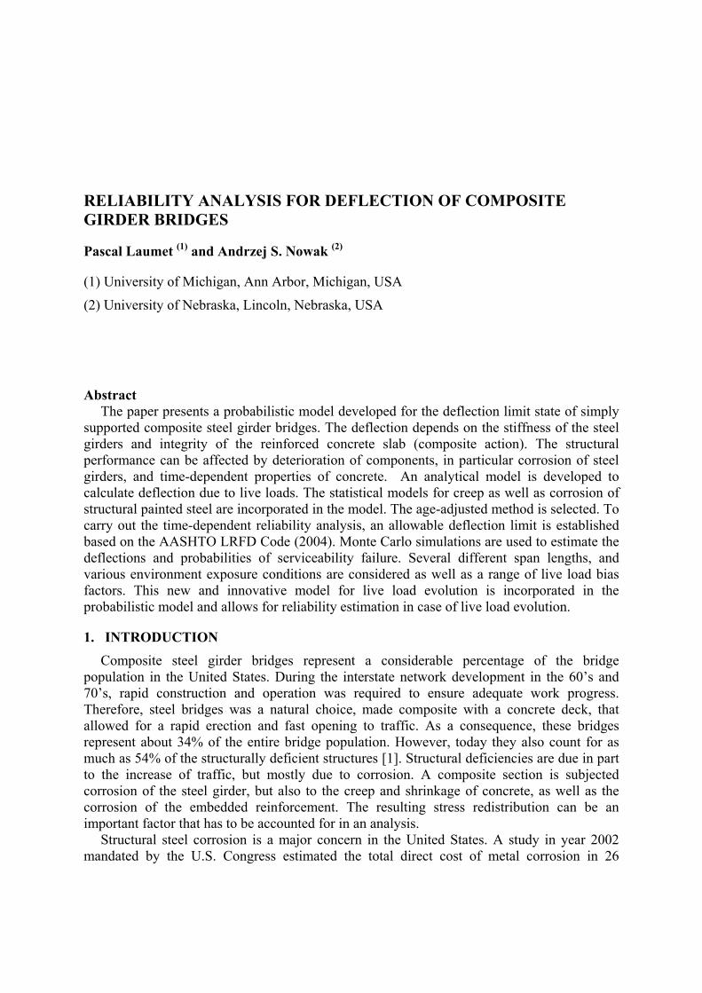
The effects of increased use of chloride-based deicing agents is dramatically illustrated by the fact that spalls were quite rare in California until late 1960s when the use of chemical deicers was introduced in this state. Another factor is the increase of salt use on highways during winter (see Fig. 1), especially in the snowbelt regions. In fact, over 70 % of the nations roads are located in snowy regions (70% of the U.S. population), which receive more than 13 cm (or 5 in.) average snowfall annually. The total amount of salt used on highways has been multiplied by 8 since 1960 and will most likely continue to grow.

Figure 1: US Highway Salts Sales Between 1940 and 2004 [3]

This paper presents a probabilistic model for reliability analysis of deflections of composite steel girder bridges including parameters such as time-dependent material properties, as well as live load evolution. The reliability analysis is based on the optional deflection serviceability limit state defined by AASHTO LRFD (2004). This serviceability failure is defined to occur when the deflection induced by live load exceeds an allowable deflection limit of length/800. Other limit states such as long-term deflections due to sustained dead load or cyclic loading, corrosion cracking, ultimate moment carrying capacity, and shear strength, are beyond the scope of the present paper.

The developed curvature-based deflection model includes the influence of instantaneous deformation due to live load as defined by the code. However, material and environmental parameters, modeling uncertainties, and live load are assumed to be random variables. Therefore, the modeled deflection is a time-dependent random variable. Monte Carlo

simulation is used to perform the reliability analysis based on the adopted allowable deflection limit.

Reliability indices (representing the probabilities of serviceability failure), are calculated for typical composite steel bridges, covering a range of realistic bridge span lengths, and the effect of live load increase is also investigated, as well as the effect of the corrosive environment.

2. DEFLECTION MODEL The analysis of time-dependent deformations of statically determinate composite beams in

bending was presented by Gilbert [4]. The deflection limit state defined in the AASHTO LRFD code (2004) only investigates the instantaneous deflections caused by the design truck portion of the live load (or 25% of the truck and lane loading, whichever is maximum). Therefore, no long-term deflection due to the sustained dead load is included in the analysis. The considered deflection is the result of a short-term load and the analysis includes time-dependent variation of the variables.

Provided that the deflections are small and that the theory of elasticity is applicable, the deflection at any point along the beam is obtained by integrating the curvature κ(x) over the length of the member, as follows

( ) dxdxxv ∫ ∫= κ (1)

where v = deflection at location x, κ(x) = curvature at any location x along the member. With an assumption of a parabolic variation of curvature, the maximum deflection Δ

occurring at midspan of a simply supported beam (see Fig. 2) can be approximated as

( ))()(10)(96

)(2

tttLt BCA κκκ ++≈Δ

96)(10)(

2Ltt Cκ≈Δ (2)

where κA(t), κB(t) = curvature at supports at time t, κC(t) = curvature at midspan at time t, Δ(t) = maximum deflection at midspan at time t, L = length of the member.

A C B

Δ

Assumed ParabolicVariation of CurvatureMoment Distribution

HS 20 defined by AASHTO LRFD

Figure 2: Deflected Shape of a Simply Supported Member under Live Load

The analysis required for deflection due to the short-term live load does not account for the time-dependent relaxation and stress redistribution due to creep and shrinkage of concrete. The strains induced by concrete relaxation under sustained loading are ignored in the present analysis since only instantaneous deflections are considered. Therefore, Eq. 2 can be reduced to its final form since the strains at supports, shrinkage-caused, are negligible. The curvature κC at any time t caused by live load can be determined as

[ ]2)()()(),()()(

tBtItAtEMtAt

eeee

eC −

=τ

κ (3)

where M = moment induced by live load, Ae(t) = equivalent area of the transformed section at time t, Be(t) and Ie(t) = first and second moment area of the transformed section at time t, Ee(t,τ) = age-adjusted effective modulus at time t, τ = age at first loading.

b

Dc

Ds

Dss

Centroid of SteelGirder Section

A ss , Iss

Transformed steelSectionAss Iss, nssnss

(a) Actual Cross-Section (b) Transformed Cross-Section

Figure 3: Actual and Transformed Cross-Section

Bazant [5] formulated a method that accounted for aging of concrete. He introduced the age-adjusted effective modulus method, sometimes called the Trost-Bazant Method. To

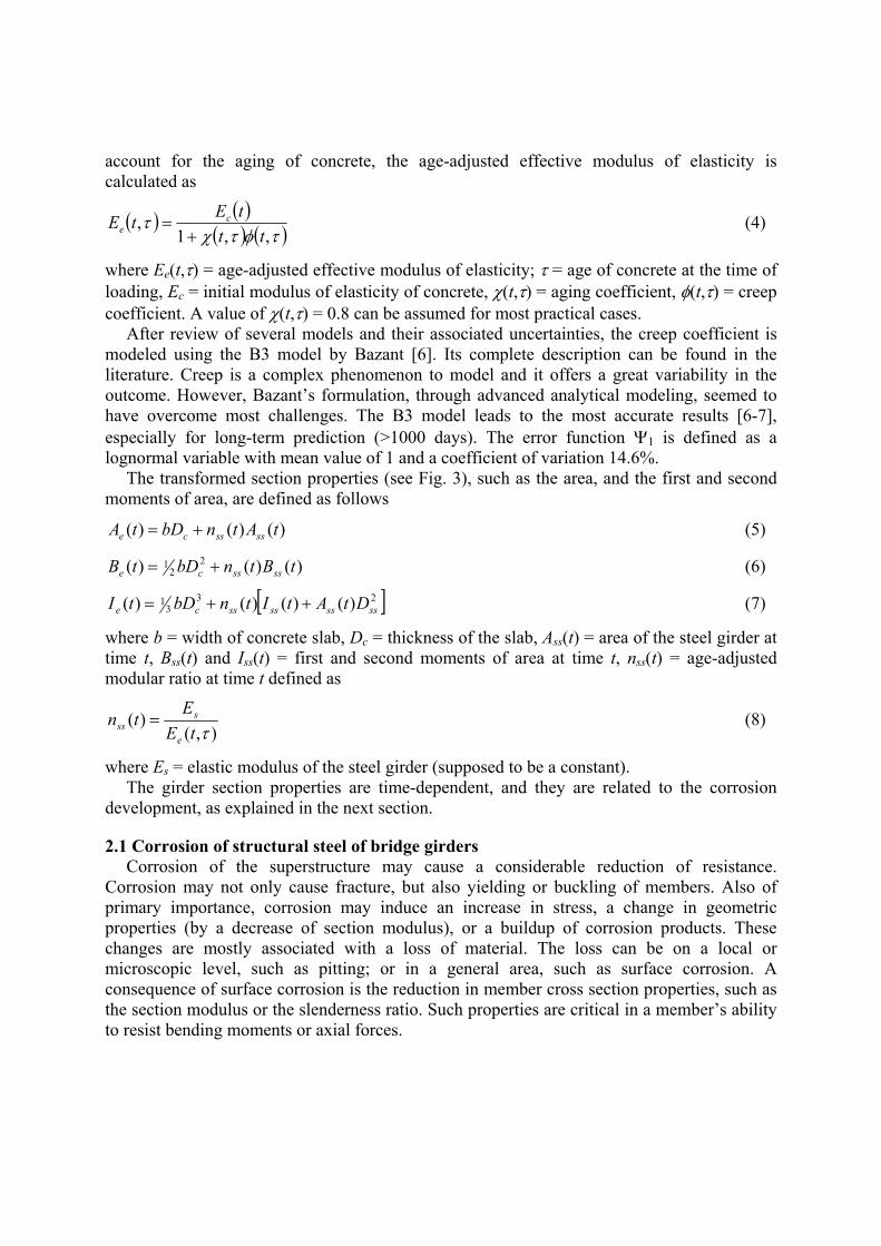
account for the aging of concrete, the age-adjusted effective modulus of elasticity is calculated as

( ) ( )( ) ( )τφτχ

τ,,1

,tt

tEtE ce +

= (4)

where Ee(t,τ) = age-adjusted effective modulus of elasticity; τ = age of concrete at the time of loading, Ec = initial modulus of elasticity of concrete, χ(t,τ) = aging coefficient, φ(t,τ) = creep coefficient. A value of χ(t,τ) = 0.8 can be assumed for most practical cases.

After review of several models and their associated uncertainties, the creep coefficient is modeled using the B3 model by Bazant [6]. Its complete description can be found in the literature. Creep is a complex phenomenon to model and it offers a great variability in the outcome. However, Bazant’s formulation, through advanced analytical modeling, seemed to have overcome most challenges. The B3 model leads to the most accurate results [6-7], especially for long-term prediction (>1000 days). The error function Ψ1 is defined as a lognormal variable with mean value of 1 and a coefficient of variation 14.6%.

The transformed section properties (see Fig. 3), such as the area, and the first and second moments of area, are defined as follows

)()()( tAtnbDtA ssssce += (5)

)()()( 22

1 tBtnbDtB ssssce += (6)

[ ]233

1 )()()()( ssssssssce DtAtItnbDtI ++= (7)

where b = width of concrete slab, Dc = thickness of the slab, Ass(t) = area of the steel girder at time t, Bss(t) and Iss(t) = first and second moments of area at time t, nss(t) = age-adjusted modular ratio at time t defined as

),()(

τtEEtn

e

sss = (8)

where Es = elastic modulus of the steel girder (supposed to be a constant). The girder section properties are time-dependent, and they are related to the corrosion

development, as explained in the next section.

2.1 Corrosion of structural steel of bridge girders Corrosion of the superstructure may cause a considerable reduction of resistance.

Corrosion may not only cause fracture, but also yielding or buckling of members. Also of primary importance, corrosion may induce an increase in stress, a change in geometric properties (by a decrease of section modulus), or a buildup of corrosion products. These changes are mostly associated with a loss of material. The loss can be on a local or microscopic level, such as pitting; or in a general area, such as surface corrosion. A consequence of surface corrosion is the reduction in member cross section properties, such as the section modulus or the slenderness ratio. Such properties are critical in a member’s ability to resist bending moments or axial forces.

Kayser and Nowak [8] established a relationship between the annual corrosion loss, the steel type and the environment exposure, based on the study by Albrecht [9]. This relationship is defined as

BAtC 2Ψ= (9)

where C = average corrosion penetration or actual corrosion loss (μm), t = number of years, A and B = parameters determined from the analysis of experimental data, Ψ1 = model error. Table 1: Average Values for Corrosion Parameters A and B, for Carbon Steel [9].

Carbon Steel Environment A B

Rural 34.0 0.65 Urban 80.2 0.59 Marine 70.6 0.79

Values of A and B depend on the environmental conditions at the bridge location, as well as the type of steel that is used (carbon mostly). In this study, the types of environment are classified as rural, urban, or marine. Average A and B values are summarized in Table 1 for unprotected carbon steel. These values were extrapolated from the results obtained from tests on small metals specimens placed on site with different exposures. Park [10] explained that the extrapolation to full-size bridges may lead to errors due to variation in component size, orientation, and local environment. Therefore, these coefficients are treated as a random variable by adding the error function Ψ1.

Carbon steel was the material of choice in the 1960’s and 1970’s, but it requires painting for corrosion protection. Even though painting provides a decent protection for 15 to 20 years, the bridges require repainting after 20-30 years (depending on the State DOT critical thresholds). The delaying effect is shown in Figure 2. Indeed, Park [10] defined three corrosion curves for painted carbon steel for three types of environment. The corrosion losses are delayed but ultimately follow the original curves (defined by Eq. 9 and Table 1). Indeed, once the paint cracks and starts to peel off, an accelerated corrosion can begin. Therefore, the relationship between the rate of corrosion and time can follow an S-shape curve. The low corrosion rate on Fig. 2 corresponds to a rural environment, medium to urban, and high to marine, respectively.

Corrosion of steel girder occurs only on the web and on the lower flange. This reduction of the steel section is taken into account in the presented analysis. Also, after review of the relevant literature [10, 11, 12], the error function �2 is defined as a lognormal variable with the mean value of 1.0 and coefficient of variation of 20%.

Figure 4: Effect of Painting on the Thickness Loss Due to Corrosion for Carbon Steel

2.2 Random parameters In the deflection analysis considered, the random parameters can be grouped into three

categories such as (1) material property parameters, (2) modeling errors, (3) applied load parameters. The dimensional properties are treated as deterministic values since their associated coefficients of variation are usually small and negligible. Materials parameters such as concrete strength fc, and concrete modulus of elasticity Ec are considered. The modeling errors have been introduced previously for the creep coefficient and corrosion predictions. The applied load parameters consider the live load only, since it governs in the short-term load analysis.

The concrete modulus of elasticity Ec is described as a random variable, but it is essentially related to the concrete compressive strength by the following formula

cc fE 4734= (10)

where fc = concrete compressive strength at 28 days (MPa). Therefore, the variation of the concrete modulus of elasticity is closely related to the concrete compressive strength.

These random variables accounts for the variability inherently associated with practical applications. The relevant statistical parameters such as the bias factor, mean value, and standard deviation are summarized in Table 2. All the presented random variables have lognormal distributions. In Table 2, the mean value of the truck loading of the live load is defined as (0.78GDF*1.79(MHS20)). In his study, Eom [14] found that the girder distribution factor defined by AASHTO can be very conservative. Based in extensive experiments, a closer value of the GDF is 0.78*GDF given by AASHTO (2004). Also, a study mandated by the Transportation Research Board in 1999 [15] has shown that the adequate bias factor for moment caused by HS20 truck loading is 1.79. It is included in the mean value for variational purpose (see Fig. 7).

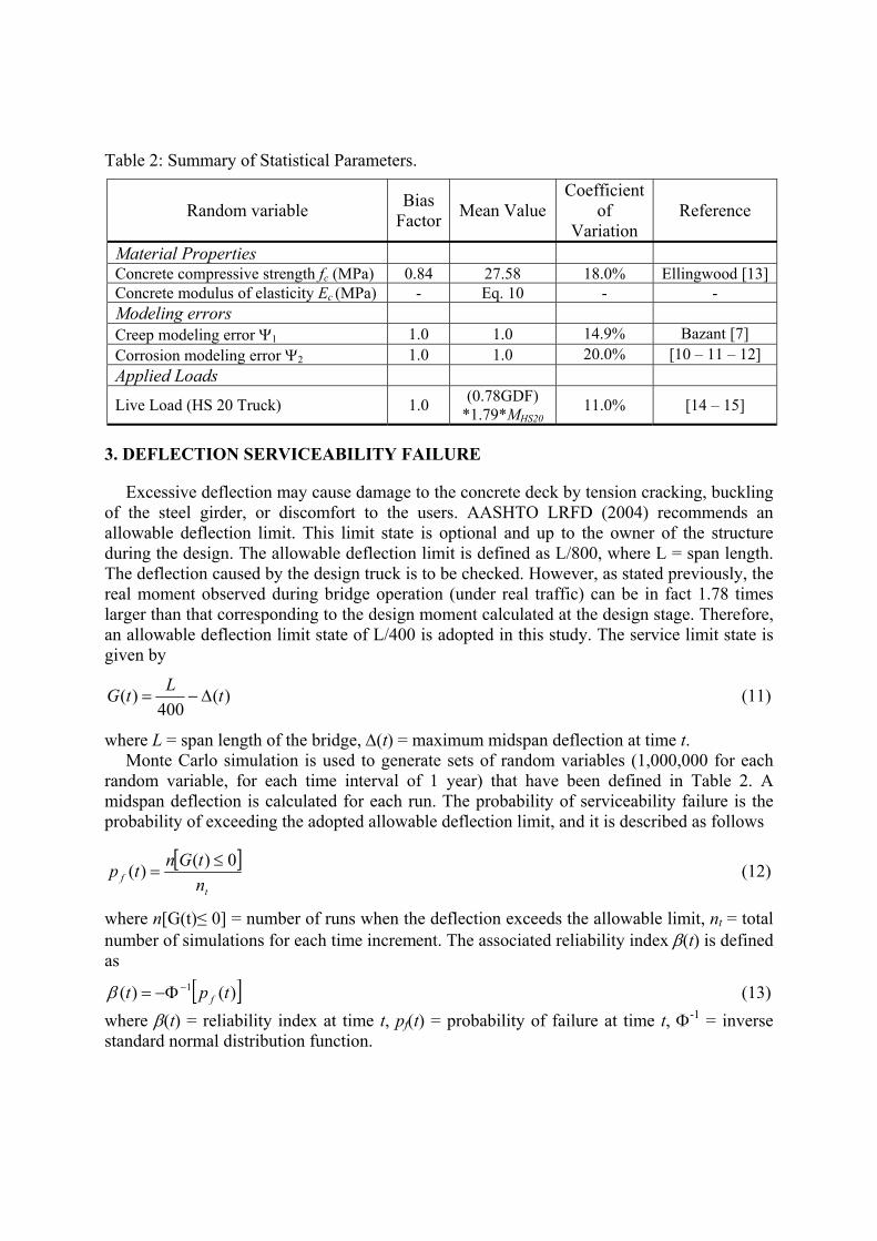
Table 2: Summary of Statistical Parameters.

Random variable Bias Factor Mean Value

Coefficient of

Variation Reference

Material Properties Concrete compressive strength fc (MPa) 0.84 27.58 18.0% Ellingwood [13] Concrete modulus of elasticity Ec (MPa) - Eq. 10 - - Modeling errors Creep modeling error Ψ1 1.0 1.0 14.9% Bazant [7] Corrosion modeling error Ψ2 1.0 1.0 20.0% [10 – 11 – 12] Applied Loads Live Load (HS 20 Truck) 1.0 (0.78GDF)

*1.79*MHS20 11.0% [14 – 15]

3. DEFLECTION SERVICEABILITY FAILURE

Excessive deflection may cause damage to the concrete deck by tension cracking, buckling of the steel girder, or discomfort to the users. AASHTO LRFD (2004) recommends an allowable deflection limit. This limit state is optional and up to the owner of the structure during the design. The allowable deflection limit is defined as L/800, where L = span length. The deflection caused by the design truck is to be checked. However, as stated previously, the real moment observed during bridge operation (under real traffic) can be in fact 1.78 times larger than that corresponding to the design moment calculated at the design stage. Therefore, an allowable deflection limit state of L/400 is adopted in this study. The service limit state is given by

)(400

)( tLtG Δ−= (11)

where L = span length of the bridge, Δ(t) = maximum midspan deflection at time t. Monte Carlo simulation is used to generate sets of random variables (1,000,000 for each

random variable, for each time interval of 1 year) that have been defined in Table 2. A midspan deflection is calculated for each run. The probability of serviceability failure is the probability of exceeding the adopted allowable deflection limit, and it is described as follows

[ ]t

f ntGntp 0)()( ≤

= (12)

where n[G(t)≤ 0] = number of runs when the deflection exceeds the allowable limit, nt = total number of simulations for each time increment. The associated reliability index β(t) is defined as

[ ])()( 1 tpt f−Φ−=β (13)

where β(t) = reliability index at time t, pf(t) = probability of failure at time t, Φ-1 = inverse standard normal distribution function.

4. EXAMPLES OF APPLICATION The structures considered are simply supported composite steel girder bridge beam

elements. A variety of length and corrosion environments are considered. They have been designed following the AASHTO LRFD (2004) design code (U.S. Units). For convenience, Table 3 summarizes the beam selection for all cases considered. Table 3: Summary of Investigated Sections.

Span (m - ft) 12.2 – 40 28.3 – 60 24.4 – 80 30.5 – 100 36.6 – 120 42.7 – 140Girder Spacing 2.43 – 8 2.43 – 8 2.43 – 8 2.43 – 8 2.43 – 8 2.43 – 8 Steel Section W24x55 W30x90 W33x130 W40x167 W40x215 W44x262

The deterministic material parameters included in the analysis are: thickness of the concrete slab hs = 22.86 cm (9 in.) – no asphalt cover; Type I cement; age at loading τ = 28 days; age when drying begins τ’ = 28 days; relative humidity H = 70% (typical in Michigan, United States); cement content = 360 kg/m3; water/cement ratio = 0.45; aggregate/cement ratio = 5.0.

The influence of the corrosion environment is shown in Fig. 5. The reliability index drops dramatically when the environment becomes harsher. Typical snow belt states such as Michigan have an environment close to the marine exposure (because of extensive use of salt as a deicing agent in winter months), which is very damaging for the structures. The effects of painting can also included.

Fig. 6 illustrates the reliability index evolution as a function of the bridge length. The AASHTO LRFD (2004), associated with the selected allowable deflection limit, provides a consistent target value between 3.5 and 4.2, depending of the degree of overdesign in the section selection.

A bias factor sensitivity analysis is performed, as shown in Fig. 7, to demonstrate its effect on the time-dependent reliability index.

In case of the growth of live load, or increase of the bias factor (ratio of actual over design load), there is a drastic drop in the reliability index (as seen in Fig. 7). For example, after 100 years, if the bias factor is increased to 1.3, then the reliability index β = 0.85, corresponding to the probability of failure of 20%.

Figure 5: Reliability Index Evolution of W90x30 for Various Environment Exposures,

(Span = 28.3 m, 60 feet; Girder Spacing = 2.43 m, 8 feet)

Figure 6: Reliability Index Evolution in Function of the Bridge Length for Urban Environment (Girder Spacing 2.43 m, 8 feet)

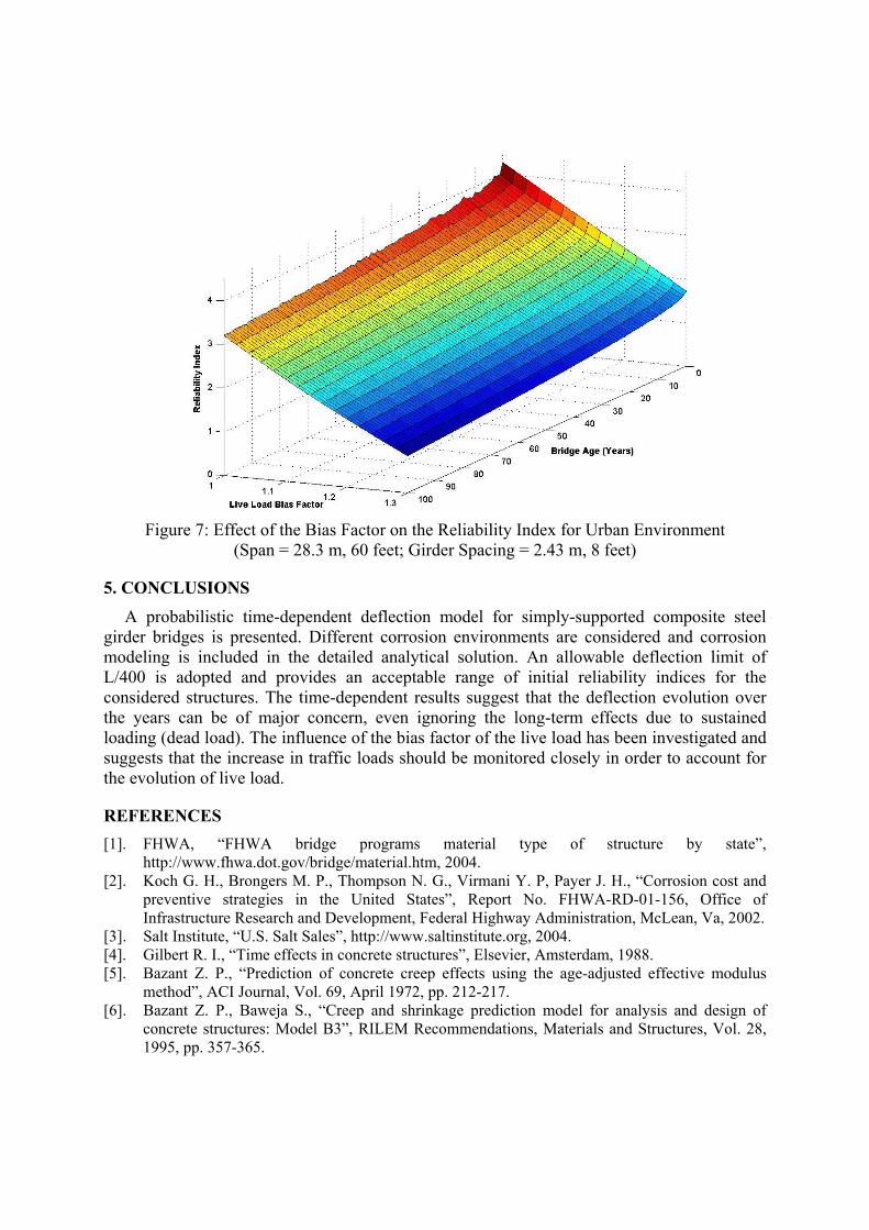
Figure 7: Effect of the Bias Factor on the Reliability Index for Urban Environment (Span = 28.3 m, 60 feet; Girder Spacing = 2.43 m, 8 feet)

5. CONCLUSIONS A probabilistic time-dependent deflection model for simply-supported composite steel

girder bridges is presented. Different corrosion environments are considered and corrosion modeling is included in the detailed analytical solution. An allowable deflection limit of L/400 is adopted and provides an acceptable range of initial reliability indices for the considered structures. The time-dependent results suggest that the deflection evolution over the years can be of major concern, even ignoring the long-term effects due to sustained loading (dead load). The influence of the bias factor of the live load has been investigated and suggests that the increase in traffic loads should be monitored closely in order to account for the evolution of live load.

REFERENCES [1]. FHWA, “FHWA bridge programs material type of structure by state”,

http://www.fhwa.dot.gov/bridge/material.htm, 2004. [2]. Koch G. H., Brongers M. P., Thompson N. G., Virmani Y. P, Payer J. H., “Corrosion cost and

preventive strategies in the United States”, Report No. FHWA-RD-01-156, Office of Infrastructure Research and Development, Federal Highway Administration, McLean, Va, 2002.

[3]. Salt Institute, “U.S. Salt Sales”, http://www.saltinstitute.org, 2004. [4]. Gilbert R. I., “Time effects in concrete structures”, Elsevier, Amsterdam, 1988. [5]. Bazant Z. P., “Prediction of concrete creep effects using the age-adjusted effective modulus

method”, ACI Journal, Vol. 69, April 1972, pp. 212-217. [6]. Bazant Z. P., Baweja S., “Creep and shrinkage prediction model for analysis and design of

concrete structures: Model B3”, RILEM Recommendations, Materials and Structures, Vol. 28, 1995, pp. 357-365.

[7]. Fabourakis G. C., Ballim Y., “Prediciting creep deformation of concrete: a comparison of results from different investigations”, Proceedings of the 11th FIG Symposium on Deformation Measurements, Santorini, Greece, 2003.

[8]. Kayser J. R., Nowak A. S., “Reliability of corroded steel girder bridges”, Structural Safety, Vol. 6, 1989, pp. 53-63.

[9]. Albrecht P., Naeemi A. H., “Performance of weathering steel in bridges”, National Cooperative Highway Research Program, Report 272, July 1984.

[10]. Park C. H., Nowak A. S., Das, P. C. ,Flint A. R.,1998, “Time-Varying Reliability Model of Steel Girder Bridges”, Proceedings Institution of Civil Engineers, Structures and Buildings, Thomas Telford Publishing, Vol. 128, Issue 4, Nov. 1998, pp. 359-367.

[11]. McCuen R. H., Albrecht P., “Composite modeling of atmospheric corrosion penetration data”, Application of Accelerated Corrosion Tests to Service Life Prediction of Materials, ASTM STP 1194, Gustavo Cragnolino and Narasi Sridhar, Eds. American Society for Testing and Materials, Philadelphia, 1994, pp. 65-102.

[12]. Melchers R. E., “Corrosion uncertainty modeling for steel structures”, Journal of Constructional Research, Vol. 52, 1999, pp. 3-19.

[13]. Ellingwood B., Galambos T. V., McGregor J. G., Cornell C. A., “Development of a probability based load criterion for American national standard A58”, National Bureau of Standards, NBS Special Publication 577, Washington D.C., 1980.

[14]. Eom J., “Verification of the bridge reliability based on field testing”, PhD Dissertation, University of Michigan, 2001.

[15]. Nowak A. S., “Calibration of LRFD Bridge Design Code”, National Cooperative Highway Research Program, NCHRP Report 368, TRB, 1999.