relaxed ziegler-nichols closed loop tuning of pi … · modeling, identi cation and control, vol....

Modeling, Identification and Control, Vol. 34, No. 2, 2013, pp. 83–97, ISSN 1890–1328

Relaxed Ziegler-Nichols Closed Loop Tuning of PIControllers

Finn Haugen 1 Bernt Lie 1

Telemark University College, Kjolnes ring 56, 3918 Porsgrunn, Norway. E-mail contact:{finn.haugen,bernt.lie}@hit.no

Abstract

A modification of the PI setting of the Ziegler-Nichols closed loop tuning method is proposed. The modifi-cation is based on a combination of the Skogestad SIMC tuning formulas for “integrator plus time-delay”processes with the Ziegler-Nichols tuning formulas assuming that the process is modeled as an “inte-grator plus time-delay” process. The resulting PI settings provide improved stability margins comparedwith those obtained with the original Ziegler-Nichols PI settings. Compared with the well-known Tyreus-Luyben PI settings, the proposed PI settings give improved disturbance compensation. For processes withzero or a negligible time-delay, but with some lags in the form of time-constants, tuning based on ultimategain and ultimate period may give poor results. Successful PI settings for such processes are proposed.

Keywords: PI controller, tuning, open loop, closed loop, Ziegler-Nichols, Tyreus-Luyben, Skogestad,relay-tuning, performance, stability, robustness.

1. Introduction

The PI (proportional plus integral) controller is prob-ably the most frequently used controller function inpractical applications. The PI controller stems froma PID controller with the D-term (derivative) deac-tived to reduce the propagation of amplified randommeasurement noise via the controller, thereby limitingvariations in the control signal due to noise.

Ziegler and Nichols (1942) presented two, now fa-mous, methods for tuning P, PI, and PID controllers:The closed loop, or ultimate gain, method, and theopen loop, or process reaction curve, method. In thepresent paper, focus is on closed loop tuning of PI con-trollers.

The PI settings with the Ziegler and Nichols closedloop method are:

Kc = 0.45Kcu (1)

Ti =Pu1.2

(2)

where Kcu is the ultimate gain, and Pu is the ultimateperiod to be found by the user. A practical, experimen-tal way to find Kcu and Pu is using relay oscillations,Astrøm and Hagglund (1995), cf. Appendix A.

It is well-known that Ziegler and Nichols closed loopPI tuning in many cases give relatively fast processdisturbance compensation, but unfortunately poor sta-bility margins, seen as poorly damped oscillatory re-sponses. This is demonstrated in several examples inSection 3. Tyreus and Luyben (1992) proposed a nowwell-known modification of the Ziegler-Nichols PI set-tings which typically give improved control system sta-bility:

Kc = 0.31Kcu (3)

Ti = 2.2Pu (4)

In the present paper, another modification of theZiegler-Nichols PI settings is proposed to provide ac-ceptable stability margins and improved disturbancecompensation compared to the Tyreus and Luyben set-tings. The proposed tuning rules, here denoted theRelaxed Ziegler-Nichols (R-ZN) PI settings, are based

doi:10.4173/mic.2013.2.4 c© 2013 Norwegian Society of Automatic Control

http://dx.doi.org/10.4173/mic.2013.2.4

Modeling, Identification and Control

on the open loop tuning rules in the SIMC method(Simple Internal Model Control) by Skogestad (2004)applied to an “integrator plus time-delay” process esti-mated from the ultimate gain and the ultimate period,Yu (1999).

The outline of this paper is as follows: In Section2, the R-ZN PI settings are derived. In Section 3, theoriginal Ziegler-Nichols (ZN) PI settings, the RelaxedZiegler-Nichols PI settings, and the Tyreus-Luyben(TL) PI settings are applied to two simulation casesand to a practical temperature control system of anair heater. In Section 4 an adjustable parameter of theR-ZN method is used to tune processes without time-delay, but with lags. Section 5 contains a discussion,and conclusions are given in Section 6.

Appendix A reviews the relay experiment of find-ing the ultimate gain and the ultimate period fromboth sinusoidal and triangular oscillations. AppendixB presents a modification of the Skogestad PI settingsfor improved disturbance compensation, used in thederivation of the proposed PI controller setting. Ap-pendix C shows abbreviations and nomenclature.

In this paper, the same symbol (letter) will be usedfor variables in time-domain as in the Laplace domain.This simplifies the notation. It is assumed that themeaning of the symbol is clear from the context.

MATLAB and SIMULINK (MathWorks, Inc.) areused for numerical computations and simulations. Lab-VIEW (National Instruments, Inc.) is used to imple-ment the temperature control system for the real airheater.

2. Relaxed Ziegler-Nichols PItuning

2.1. Derivation of the tuning formulas

The following PI controller function is assumed:

u (t) = uman +Kce (t) +Kc

Ti

∫ t

0

e (τ) dτ (5)

Skogestad (2004) has provided PI settings for a num-ber of different types of process dynamics, amongwhich are “integrator plus time-delay” and “time-constant plus time-delay”. Assuming that Skogestad’srule-of-thumb about setting the user-specified closedloop time-constant, Tc, equal to the process time-delay,τ , his PI settings for these two process types are actu-ally identical as long as the relation between the time-constant of the “time-constant plus time-delay” pro-cess and the time-delay satisfies

T ≥ 8τ (6)

In the following, it is assumed that eq. (6) is satisfiedfor the process to be controlled. Thus, an “integratorplus time-delay” process is assumed, with the followingtransfer function:

∆y(s)

∆u(s)= Hp(s) =

Kip

se−τs (7)

The Skogestad PI settings for this process are:

Kc =1

Kip (Tc + τ)(8)

Ti = cs (Tc + τ) (9)

The parameter cs is introduced here. The original PIsettings in Skogestad (2004) correspond to cs = 4 ineq. (9). For “integrator plus time-delay” processeswith an “input” process disturbance, the disturbancecompensation appears as unnecessarily slow with cs =4. To obtain a faster disturbance compensation whileretaining acceptable stability margins, a value of cssmaller than 4 can be used. It is found that valuesaround 2 are proper values. Thus, cs = 2 is proposed.The implications of various values of cs are investigatedin Appendix B.

The user must select a proper value of Tc in eqs.(8) and (9). Skogestad provides the following rule-of-thumb:

Tc = τ (10)

With cs = 2 and the rule-of-thumb eq. (10), eqs. (8)and (9) become

Kc =1

2Kipτ(11)

Ti = 4τ (12)

which may be denoted the modified Skogestad PI set-tings for “integrator plus time-delay” processes.

The Skogestad PI settings, also with cs = 2, typicallyyield acceptable stability of the control system, whileZiegler and Nichols PI settings often give poor stability,with oscillatory responses (as demonstrated in severalapplications in Section 3). The PI settings, eqs. (11)and (12), will now be exploited to relax the original ZNPI settings, eqs. (1)-(2).

For an “integrator plus time-delay” process, Kip andτ can be estimated from Kcu and Pu as follows, Yu(1999), DiRuscio (2010):

Kip =2π

KcuPu(13)

τ =Pu4

(14)

As pointed out in Seborg et al. (2004), process param-eters Kip and τ can be used in any model-based con-troller tuning method. Here, the (modified) Skogestad

84

F. Haugen and B. Lie “Relaxed Ziegler-Nichols Closed Loop Tuning of PI Controllers”

PI settings, eqs. (11) and (12), are used. Inserting eqs.(13) and (14) into eqs. (11) and (12) gives

Kc =Kcu

π= 0.32Kcu (15)

Ti = Pu (16)

which will be referred to as the (default) RelaxedZiegler-Nichols (R-ZN) PI settings.

Comparing with ZN and TL

Compared with the (original) ZN PI settings, eqs. (1)-(2), the gain is smaller and the integral time is some-what larger in the R-ZN PI settings, indicating im-proved stability.

Compared with the TL PI settings, eqs. (3)-(4), theR-ZN gain is almost the same, while the R-ZN integraltime is smaller, indicating faster integral action, i.e.the control error is brought faster to zero, however,somewhat reduced stability can be expected.

Enhanced relaxation

Above, the closed loop time-constant is set equal tothe (estimated) process time-delay, cf. eq. (10). Par-ticularly in applications where the process has zero ornegligible time-delay but some lag, the default R-ZNPI settings may result in poor stability (and the ZNsettings may even give instability). Acceptable stabil-ity can be obtained with enhanced relaxation of the PIsettings. To this end, we propose

Tc = krτ (17)

where kr ≥ 1 is a relaxation parameter to be set bythe user. The default PI settings, eqs. (6) and (6), areobtained with kr = 1. Enchanced relaxation of the PIsettings is obtained with kr > 1. Using eq. (17) in eqs.(8) and (9), and setting cs = 2 in (9), give

Kc =2

π (kr + 1)Kcu (18)

and

Ti =kr + 1

2Pu (19)

The usefulness of enhanced R-ZN tuning is demon-strated in Section 4.

One question may arise: Why not just apply origi-nal ZN settings and adjust Kc and Ti directly? Whilethis is of course an option, we think that it better touse a meaningful single parameter, kr, to obtain the PIsettings. The benefit of reducing the number of con-troller parameters to adjust from two to one is actuallysubstantial. Skogestad’s tuning method is an excellent

example of this: From the user’s perspective, adjustingTc, which has a meaningful interpretation, to obtainthe PI settings is a much simpler task than adjustingKc and Ti directly.

2.2. Some derived results

Estimation of control system response-time

The control system response-time, Tr, can be estimatedfrom the ultimate period, Pu, as explained in the fol-lowing. The typical setting of kr = 1 is here assumed.Then the PI settings are eqs. (6) and (6). Assume thatthe setpoint is changed as a step. Then the responsein the process output reaches 63% of its final value attime (approximately)

Tr ≈ τ + Tc =Pu4

+Pu4

=Pu2

(20)

Tr is here the 63% rise-time, or response-time, of thecontrol system. As an example of eq. (20), see Figure9 where the response in air heater temperature due toa setpoint step is plotted. In that example, Pu = 15 s,giving Tr ≈ Pu/2 = 7.5 s, which is in good accordancewith the plotted response in Figure 9.

Retuning the PI controller

Equations (18) and (19) can be used to retune a PIcontroller safely. Note that the factor (kr + 1) appearsin the denominator of eq. (18) and in the numeratorof eq. (19). For example, assume that it is desired todecrease the present value of Kc by a factor of 2 (toobtain a smoother control signal). This gain reductionshould be acccompanied by an increase of Ti by a factor2. (This inversely proportional adjustment also followsdirectly from Skogestad’s formulas, eqs. (8) and (9).)

3. Applications

3.1. Overview

In the following subsections, PI settings with the (orig-inal) Ziegler-Nichols closed loop method, the R-ZNclosed loop method, and the TL method are appliedto the following three cases:

• A simulated control system for an “integrator withtime-delay” process (Section 3.3).

• A simulated control system for a “time-constantwith time-delay” process (Section 3.4).

• A practical temperature control system for a lab-oratory air heater (Section 3.5). The processdynamics is roughly “time-constant with time-delay”.

85


The PI settings will be compared using quantitivemeasures of performance and robustness defined in Sec-tion 3.2.

For easy reference, the various PI settings formulasare summarized in Table 1. In the examples, Kcu andPu are found from the method of relay oscillations de-scribed in Appendix A.

Table 1: PI settings formulas.

ZN R-ZN TLKc 0.45Kcu 0.32Kcu 0.31Kcu

TiPu

1.2 Pu 2.2Pu

3.2. Measures of performance androbustness

The measures used in this paper for comparing thevarious methods of PI controller tuning can be groupedinto performance and robustness measures described inthe detail in the following.

3.2.1. Performance

IAE at setpoint change

In the tests the setpoint is changed as a step. Thesetpoint tracking is measured with the IAE (Integralof Absolute Error) index calculated over a proper timeinterval as

IAEs =

∫ tf

ti

|e| dt (21)

where e is the control error, ti is the initial time, se-lected as the time of the step change, and tf is a properfinal time. A reduced IAEs value indicates improvedsetpoint tracking.

IAE at process disturbance change

In the tests a process disturbance is changed as a step.The disturbance compensation is measured with

IAEd =

∫ tf

ti

|e| dt (22)

A reduced IAEd value indicates improved disturbancecompensation.

Response time

The response time, Tr [s], is here defined as the inverseof the bandwidth defined as the amplitude crossoverfrequency, ωc [rad/s]:

Tr =1

ωc(23)

Tr indicates the speed of the response of the controlsystem due to a setpoint step change. Tr is approxi-mately the time-constant of the control system. ωc isequal to the phase crossover frequency, ω180d

, of theloop brought to marginal stability by a reduction ofthe phase of the loop while the amplitude is retained,as by an increase of the loop time-delay:

Tr =1

ω180d

=Pu2π

(24)

where Pu [s] is the (ultimate) period of the oscillationsat marginal stability.

Setpoint tracking versus disturbance compensation

For systems where the setpoint is constant, which isthe case in many practical process control systems, itcan be claimed that good disturbance compensation ismore important than good setpoint tracking. In the ex-amples presented in the following sections, disturbancecompensation is emphasized.

3.2.2. Stability robustness (stability margins)

Gain margin, GM

For the cases based on simulations GM is calculatedfrom the loop transfer function, HL(s), using the mar-gin function in MATLAB. HL(s) is

HL(s) = Hc(s)Hp(s) (25)

where Hc(s) is the controller transfer function, andHp(s) is the process transfer function.

For the practical case (air heater) an adjustable gain,∆K, is inserted into the loop (between the controllerand the process), see Figure 1. Initially, ∆K = 1. The

Process

w/actuator

and sensor

and filter

ySP Cont-

roller

d

ymfuDK (t-Dt)

Adjustable

gain

Adjustable

time-delay

Disturbance

Process

measurementSetpoint

Figure 1: An adjustable gain and time-delay are in-serted into the loop to find the stabilitymargins (gain margin and phase margin)experimentally.

(ultimate) value ∆Ku that brings the control system tothe stability limit so that the responses are sustainedoscillations, is found experimentally (by trials). Thegain margin is then

GM = ∆Ku (26)

86


Phase margin, PM

For the cases based on simulations PM is calculatedfrom the loop transfer function using the margin func-tion in MATLAB.

For the practical case (air heater) an adjustable time-delay, ∆τ [s], is inserted into the loop (between thecontroller and the process), see Figure 1. Initially,∆τ = 0. For each of the tuning methods, the value ∆τuthat brings the control system to the stability limit, i.e.causing sustained oscillations, is found experimentally.The period, Pu [s], of the oscillations is measured. Thecorresponding phase margin is

PM [deg] = 360∆τuPu

(27)

Equation (27) is derived in Haugen (2012) (Ap-pendix 1).

Proper values of GM and PM

Seborg et al. (2004) propose the following ranges forproper values of the stability margins:

1.7 = 4.6 dB ≤ GM ≤ 4.0 = 12.0 dB (28)

and30o ≤ PM ≤ 45o (29)

Since poor control system stability must be avoided,the lower limits of GM and PM can be regarded ascritical, while the upper limits are not.

3.3. Application: Simulated “integratorplus time-delay” process

3.3.1. Process description

The process to be controlled is an “integrator plustime-delay” process:

y(t) = Kipu(t− τ) +Kdd(t) (30)

which has transfer function as in eq. (7). The processparameter values are: Kip = 1 s−1, Kd = 1, τ = 1 s.

3.3.2. PI controller tuning from relay oscillations

Kcu and Pu are found from relay oscillations. Figure 2shows plots of the sustained oscillations during the re-lay tuning, cf. Appendix A. From the plots,Atri = 1.0.The square wave in the control signal has amplitudeAsq = 1.

Equation (47) in Appendix A gives

Kcu =πAsq2Atri

=π · 12 · 1

= 1.57 (31)

0 5 10 15 20 25 30−2

−1

0

1

2

ysp

: red. y: blue.

0 5 10 15 20 25 30−1

−0.5

0

0.5

1

u

0 5 10 15 20 25 30−1

−0.5

0

0.5d

t [s]

Figure 2: Responses during relay tuning

It is interesting that the ultimate gain using a P con-troller also gives Kcu = 1.57. Hence, the Fourier-seriesapproximations used to derive eq. (47) give a very pre-cise result in this case.

Furthermore, from the plots,

Pu = 4.0 s (32)

Various PI settings are calculated from the abovevalues of Kcu and Pu using the formulas in Table 1.The PI settings are shown in Table 2.

3.3.3. Performance and stability robustness of thecontrol system

Figure 3 shows responses in the process output variable(y) and the controller output (u) with a step changeof the temperature setpoint (ysp) and a step change ofthe disturbance (d) for the three different PI settingsshown in Table 2.

GM, PM and Tr are calculated from the model.IAEs is calculated time-series over the interval t =[2 s, 40 s]. IAEd is calculated over t = [40 s, 80 s].Table 2 summarizes the performance and robustnessmeasures.

Below are a number of observations made in Table 2(the abbreviations are as in Table 2):

• Setpoint tracking :

IAEs: ZN and TL are the best, and almost equal,but ZN suffers from large overshoot.

87


0 10 20 30 40 50 60 70 800

1

2

3

4

ysp

: Red. y: ZN: Blue; relaxed ZN: Black; TL: Magenta

0 10 20 30 40 50 60 70 80−1

0

1

2u: ZN: Blue; relaxed ZN: Black; TL: Magenta

0 10 20 30 40 50 60 70 80−1

−0.5

0

0.5d

t [s]

Figure 3: Responses with various PI settings.

Table 2: Controller settings and performance and ro-bustness measures for simulated control sys-tem for ”integrator plus time-delay” processwith different PI settings.

ZN R-ZN TLKc 0.71 0.50 0.49Ti [s] 3.3 4.0 8.8IAEs 7.9 8.1 8.0IAEd 2.8 4.5 9.0GM 1.9 2.7 3.1

GM [dB] 5.4 8.8 9.7PM [deg] 24.9 34.1 48.6Tr [s] 1.3 s 1.8 2.0

Tr: ZN is the best, while R-ZN and TL do notdiffer much.

• Disturbance compensation:

IAEd: ZN is clearly best. R-ZN is in turn clearlybetter than TL as the R-ZN has a value which is50% of the value of TL.

• Stability robustness (margins):

GM: ZN is poor, and actually below the lower limitin ineq. (28). R-ZN and TL do not differ muchand have acceptable values.

PM: Again ZN is poor, and below the lower limitin ineq. (29). R-ZN gives a somewhat small, butacceptable, value. TL gives large value, possibly

unnecessarily large as it is larger than the higherlimit in ineq. (29).

The low stability margins with ZN are apparentin the oscillatory responses with the ZN settings,see Figure 3.

Comments and conclusions

The Ziegler-Nichols PI settings give poor control loopstability margins. The TL and the R-ZN settings giveacceptable stability margins. With emphasis on dis-turbance compensation rather than setpoint tracking,the R-ZN settings are better than the TL settings.

3.4. Application: Simulated“time-constant plus time-delay”process


The process to be controlled is a “time-constant plustime-delay” process (assuming the time-delay is at theinput-side):

T y(t) = −y(t) +Ku(t− τ) +Kdd(t) (33)

The process parameter values are: K = 8, Kd = 8, τ =1 s.

The time-constant being 8 times the time-delaymakes the Skogestad PI settings for a “time-constantplus time-delay” process become identical with thesettings for an “integrator plus time-delay” process.Therefore, the condition for using Skogestad tuningfor “integrator plus time-delay” processes, ineq. (6),is satisfied.


The ultimate gain and the ultimate period are foundfrom relay oscillations. Figure 4 shows plots of thesustained oscillations during the relay tuning. The re-sponse in y are approximately triangular, so eq. (47)is used to calculate Kcu . From Figure 4,Atri = 0.94,Asq = 1. Equation (47) gives

Kcu =πAsq

2Atri=π · 0.94

2 · 1= 1.48 (34)

The ultimate gain using a P controller gives Kcu = 1.65which differs somewhat from 1.48. Still, Kcu = 1.48 isused to stick to relay tuning, and using 1.48 ratherthan 1.65 is safe (conservative) regarding control loopstability.

Furthermore, from Figure 4,

Pu = 3.78 s (35)

88


0 5 10 15 20 25 30−1

−0.5

0

0.5

1

ysp

: red. y: blue.

0 5 10 15 20 25 30−1

−0.5

0

0.5

1

u

0 5 10 15 20 25 30−1

−0.5

0

0.5d

t [s]


Various PI settings are calculated from the abovevalues of Kcu and Pu using the formulas in Table 1.The PI settings are shown in Table 2.


Figure 5 shows responses in the process output variable(y) and the controller output (u) with a step changeof the temperature setpoint (ysp) and a step change ofthe disturbance (d) for the three different PI settingsshown in Table 3.

GM, PM and Tr are calculated from the model. IAEsis calculated over the interval t = [2 s, 40 s]. IAEd iscalculated over t = [40 s, 80 s]. Table 3 summarizesthe performance and robustness measures.

Table 3: Controller settings and performance and ro-bustness measures for simulated control sys-tem for ”time-constant plus time-delay” pro-cess with different PI settings.

ZN R-ZN TLKc 0.75 0.53 0.52Ti [s] 3.2 3.8 8.3IAEs 6.1 5.8 4.3IAEd 2.1 3.6 7.9GM 1.7 2.6 3.0

GM [dB] 4.8 8.1 9.7PM [deg] 22.3 32.2 60.1Tr [s] 1.2 1.7 1.9

0 10 20 30 40 50 60 70 800

1

2

3

ysp


0 10 20 30 40 50 60 70 80−1

0

1

2u: ZN: Blue; relaxed ZN: Black; TL: Magenta

0 10 20 30 40 50 60 70 80−1

−0.5

0

0.5d

t [s]




IAEs: TL is best.

Tr: ZN is best, while R-ZN and TL do not differmuch.


IAEd: ZN is clearly best. R-ZN is in turn clearlybetter than TL. R-ZN has a value which is 45 %of the value of TL.


GM: Strictly, all settings give acceptable values,but ZN is on the lower limit.

PM: ZN is poor, and below the lower limit in ineq.(29). R-ZN gives a somewhat small, but accept-able, value. TL gives a large value, possibly unnec-essarily large as it is larger than the higher limitin ineq. (29).


The Ziegler-Nichols PI settings give poor control loopstability as the PM is too small. The rest of the com-ments are identical with those for the “integrator plustime-delay” case in Section 3.3: The TL and the R-ZNsettings give acceptable stability margins. With em-phasis on disturbance compensation rather than set-point tracking, the R-ZN settings are better than theTL settings.

89


3.5. Application: Practical temperaturecontrol system


Figure 6 shows an air heater laboratory station. The

Figure 6: Temperature control system for an air heater(laboratory rig)

temperature of the air outlet is controlled by adjustingthe control signal (voltage) to the heater. The temper-ature is measured with a Pt100 element. A measure-ment filter with time-constant 0.5 s is used to attenuatemeasurement noise. The National Instruments USB-6008 is used as analog I/O device. The control systemis implemented in LabVIEW (National Instruments)running on a PC. The fan rotational speed, and the airflow, can be adjusted manually with a potentiometer.Changes of the air flow comprises a process disturbancegiving an impact on the temperature. The measuredvoltage drop across the potensiometer is representedby the variable F in percent. Thus, F represents theair flow disturbance.1

The nominal operating point of the system is tem-perature at 35 oC and air flow F = 50 %.

Figure 7 shows the open loop, or process, step re-sponse in the filtered temperature, ymf , due to a stepin the heater control signal, u. The response indicatesthat the process dynamics is roughly “time-constantwith time-delay”, with time-constant ≈ 37 s and time-delay ≈ 3 s which is about 8% of the time-constant.

1 Additional information about the air heater is available atHaugen (2013).

120 140 160 180 200 220 240 260 280 300 32034

35

36

37

38

39

ymf

[Deg C

]120 140 160 180 200 220 240 260 280 300 320

0

1

2

3

4

5

u

[V]

t [s]

Figure 7: Open loop step response in filtered tempera-ture, ymf , due to a step in the heater controlsignal, u.


Kcu and Pu are found from relay oscillations. Figure8 shows plots of the sustained oscillations during therelay tuning. The oscillations in temperature (processmeasurement) looks more sinusoidal than triangular.Therefore, Kcu is calculated using eq. (45).

From Figure 8, Asin = 0.75 oC and Asq = 2.5 V.Equation (45) gives

Kcu =4Asq

πAsin=

4 · 2.5 V

π · 0.75 oC= 4.24

VoC

(36)

From Figure 8,

Pu = 15.0 s (37)

Various PI settings are calculated from the abovevalues of Kcu and Pu using the formulas in Table 1.The PI settings are shown in Table 4. Both standard R-ZN and enhanced R-ZN tuning are applied, with kr = 1and kr = 2, respectively.


Figures 9, 10, 11, and 12 show responses in the airtemperature (ymf ) and the controller output (u) dueto a step change of the temperature setpoint (ysp) and astep change of the disturbance (d) for the four differentPI settings shown in Table 4.

90


100 110 120 130 140 150 160 170 180 190 20033

34

35

36

37

ysp

: Red. ymf

: Blue.

[Deg C

]

100 110 120 130 140 150 160 170 180 190 200

0

1

2

3

4

5

u

[V]

t [s]


Performance and stability robustness measures arecalculated from the time-series as explained in Sec-tion 3.2. IAEs is calculated over the intervalt = [100 s, 180 s]. IAEd is calculated over t =[200 s, 280 s]. Table 4 summarizes the performanceand robustness measures.

Table 4: Controller settings and performance and ro-bustness measures for practical temperaturecontrol system for different PI settings.

ZNR-ZNkr = 1

R-ZNkr = 2

TL

Kc 1.91 1.35 0.90 1.32Ti [s] 12.5 15.0 22.5 33.0IAEs 16.2 12.3 10.6 10.3IAEd 4.3 4.9 7.5 11.8GM 1.5 1.8 2.8 2.6

GM [dB] 3.5 5.1 8.9 8.3∆τu [s] 1.6 2.6 7.7 5.7Pu [s] 24.0 31.0 50.0 39.0

PM [deg] 24.0 30.2 55.4 52.6Tr [s] 3.8 4.9 8.0 6.2



IAEs: TL and R-ZN with kr = 1 and with kr = 2do not differ much and are clearly better than ZNwhich is due to the large overshoot and oscillatoryresponse with ZN.

80 100 120 140 160 180 200 220 240 260 280 30034.5

35

35.5

36

36.5

37

ysp

: Red. ymf

: Blue.

[Deg C

]

80 100 120 140 160 180 200 220 240 260 280 3000

1

2

3

4

5u

[V]

80 100 120 140 160 180 200 220 240 260 280 3000

50

100

d (air flow)

[%]

t [s]

Figure 9: Responses with Ziegler-Nichols PI settings

Tr: ZN is clearly best. It gives fast control. R-ZNwith kr = 1 is also relatively fast.


IAEd: ZN and R-ZN with kr = 1 are much betterthan both R-ZN with kr = 2 and TL. R-ZN withkr = 1 give only 36% of that of TL. Relaxed ZNwith kr = 2 is also clearly better than TL.


GM: ZN is poor, and actually below the lower limitin ineq. (28). R-ZN with kr = 1 is small, but justwithin the limits.

PM: Again ZN is poor, and below the lower limitin ineq. (29). R-ZN with kr = 1 is small, butjust within the limits. TL has a large value, pos-sibly unnecessarily large since it is larger than thehigher limit in ineq. (29). R-ZN with kr = 2 hasa very large value.

The low stability margins with ZN are apparent inthe oscillatory responses with the ZN settings. R-ZN with kr = 1 seems to give acceptable stabilityas seen from time-series. R-ZN with kr = 2 andTL both give smooth, but slow, responses.


The Ziegler-Nichols PI settings give poor control loopstability. The TL and the R-ZN settings both withkr = 1 and kr = 2 give acceptable stability margins,though R-ZN with kr = 1 gives small margins. R-ZN

91


80 100 120 140 160 180 200 220 240 260 280 30034.5

35

35.5

36

36.5

37

ysp

: Red. ymf

: Blue.

[Deg C

]

80 100 120 140 160 180 200 220 240 260 280 3000

1

2

3

4

5u

[V]

80 100 120 140 160 180 200 220 240 260 280 3000

50

100

d (air flow)

[%]

t [s]

Figure 10: Responses with R-ZN PI settings with kr =1.

with kr = 1 give clearly the best disturbance compen-sation, and since the stability margins are within theacceptable limits, it gives the prefered PI settings inthis application.

If it is important with smooth responses, both TLand R-ZN with kr = 2 can be used. Among these two,we prefer the latter because it gives best disturbancecompensation, and because the R-ZN settings are ad-justable, while the TL settings are fixed.

4. Relaxed tuning for processeswith no time-delay but with lags

Closed loop PI tuning with the standard Ziegler-Nichols method, the TL method, or even the R-ZNtuning method with the default setting kr = 1 maynot work well if the process has no, or negligible time-delay, however, some lag is assumed. The resultingstability may be very poor. Such cases may occur ine.g. temperature control, Haugen et al. (2013) and bio-gas flow control of bioreactors, Haugen and Lie (2013).However, enhanced R-ZN tuning with a proper kr > 1seems to work well. An explanation of the resultingpoor stability is that, due to the lack of a time-delay,the phase characteristic is relatively flat around thecritical frequencies, making the phase margin small.

Now, an extreme case is assumed, and enhanced R-ZN PI tuning is used. The value of kr that is founduseful in this case may be used in other less extreme

80 100 120 140 160 180 200 220 240 260 280 30034.5

35

35.5

36

36.5

37

ysp

: Red. ymf

: Blue.

[Deg C

]

80 100 120 140 160 180 200 220 240 260 280 3000

1

2

3

4

5u

[V]

80 100 120 140 160 180 200 220 240 260 280 3000

50

100

d (air flow)

[%]

t [s]

Figure 11: Responses with R-ZN PI settings with kr =2.

cases to obtain proper stability. Note that for processeswith a noteable time-delay the R-ZN PI settings withthe default value kr = 1, i.e. eqs. (6)-(6), should beused.

Assume that the process is an integrator withoutany time-delay but with two lags in the form of time-constant terms where one of the time-constants is onetenth of the other. Specifically, the following processtransfer function model is assumed:

y(s) =1

s(T1s+ 1)(T2s+ 1)

[Kipu(s) +Kdd(s)

](38)

where u is control variable and d is disturbance. Time-constant T1 may represent a process lag due to e.g.dynamics of a heating element or a valve or a pump orrepresent inhomogeneous conditions in a tank, whileT2 may represent the time-constant of a measurementfilter. The integrator, 1/s, may represent e.g. energyor material balance. The following parameter valuesare assumed: Kip = 1 s−1 Kd = 1, T1 = 1 s, andT2 = 0.1 s. In less extreme cases the difference betweenthe two time-constants are less, and there may also bea non-zero time-delay.

The relay method is used, giving Kcu = 10.24 andPu = 2.02 s. The three PI tuning methods mentionedin the beginning of the present section are tested. Fig-ure 13 shows their responses. With TL tuning andR-ZN tuning with kr = 1 the control system is stable,but the stability is poor. With Ziegler-Nichols tuning,the system is unstable!

92


80 100 120 140 160 180 200 220 240 260 280 30034.5

35

35.5

36

36.5

37

ysp

: Red. ymf

: Blue.

[Deg C

]

80 100 120 140 160 180 200 220 240 260 280 3000

1

2

3

4

5u

[V]

80 100 120 140 160 180 200 220 240 260 280 3000

50

100

d (air flow)

[%]

t [s]

Figure 12: Responses with TL PI settings

0 5 10 15−1

−0.5

0

0.5

1

1.5

2

2.5

3

ysp


t [s]


By trial-and-error it is found that R-ZN tuning withkr = 4 works well. Hence, with kr = 4 in (18) and (19)the PI settings become

Kc = 0.13Kcu (39)

andTi = 2.5Pu (40)

Figure 14 shows simulated responses. Table 5 showsPI settings and stability margins.

Comments and conclusion:

• GM is large, but is accepted here.

• PM is small and just outside the acceptable rangewhere 30.0o is the critical limit, cf. ineq. (29).

0 10 20 30 40 50 60 70 800

0.5

1

1.5

2

ysp

: Red. y: ZN: Blue

0 10 20 30 40 50 60 70 80−1

0

1

2u

0 10 20 30 40 50 60 70 80−1

−0.5

0

0.5d

t [s]

Figure 14: Responses with PI controller tuned with theR-ZN method with kr = 4.

Table 5: Controller settings and performance and ro-bustness measures for simulated PI controlsystem for an ”integrator with two lags” pro-cess with R-ZN tuning with kr = 4.

Kc 1.3Ti [s] 5.2GM 6.7

GM [dB] 16.5PM [deg] 29.4

However, the value of 29.4o is here regarded asacceptable since it is for an assumed extreme case.With kr = 5 PM = 34.3o which is within the rangegiven by ineq. (29), but simulations indicate thatthe control system becomes unnecessarily sluggishwith kr = 5 applied for less extreme cases.

• How can one know that a process has one or morelags and no or negligible time-delay, so that theenhanced relaxed tuning should be applied? Phys-ical insight may be useful: If the sensor or actuatoris located close to the main process (which can bee.g. a reactor vessel), the time-delay may be neg-ligible compared to time-constant lags. A processstep response test is also an option, but then anopen loop controller tuning method, as the Skoges-tad method (2003, 2004), may be applied directly.

93


5. Discussion

The proposed new set of PI settings are based on tun-ing rules derived by Ziegler and Nichols (1942), tuningrules derived by Skogestad (2004), and the modelingof the process as an “integrator plus time-delay” ac-cording to Yu (1999). The validity and applicabilityof the proposed PI settings rely on assumptions madeby these authors. The sensitivity of the present resultswith respect to such assumptions has not been inves-tigated here. However, two simulation tests and onepractical test indicate that the proposed tuning worksas assumed.

In the simulations it is assumed that the processdisturbance is an input disturbance as it acts on theprocess at the same place, dynamically, as the controlsignal does. In most practical processes the main dis-turbances are actually input disturbances. We have notinvestigated the consequences for our results of movingthe disturbance to the process output.

It is found that for processes with no, or a negligibletime-delay, but with some lags in the form of time-constants, R-ZN tuning with kr = 1 may give poorstability (This applies to ordinary ZN and TL tuning,too). However, proper stability may be obtained withenhanced relaxation of the tuning, and kr = 4 seems tobe a proper value at least for processes without time-delay but with two lags with one being one tenth of theother. The conditions that make the selection kr = 4unsuccessful have not been investigated, but for pro-cesses where the time-constants are closer, the PI set-tings with kr = 4 will certainly be safe (conservative).

6. Conclusions

The main result of this paper is a proposed new set ofPI settings which uses the same information as in theZiegler-Nichols closed loop method, namely knowledgeabout the ultimate gain, Kcu , and the ultimate period,Pu: The proposed settings are:

Kc = 0.32Kcu

Ti = Pu

These settings are modifications, or relaxations, of theoriginal Ziegler-Nichols PI settings, and they give im-proved control system stability. In this paper, the pro-posed setting have been successfully applied to two sim-ulated control systems and to a practical temperaturecontrol system of an air heater.

Comparing with the TL PI settings, which also arebased on knowledge of the ultimate gain and the ul-timate period, the proposed PI settings give clearlybetter disturbance compensation.

The proposed PI settings have an adjustable param-eter which can be used to obtain enhanced relaxationwhich is useful for processes with zero or negligibletime-delay but some lags (time-constants).

Acknowledgments

Telemark University College has provided practicaland economical support for the work with this paper.Thanks to colleague David Di Ruscio for useful discus-sions.

A. Finding the ultimate gain andperiod from relay oscillations

In the original Ziegler-Nichols closed loop method theuser must find, typically by trial-and-error, the ulti-mate controller gain value, Kcu , of a P controller whichmakes the responses in the control system become sus-tained oscillations. The user must also read off theultimate period, Pu, of the oscillations. Kcu and Puare then used to calculate the PI settings with the fol-lowing formulas:

Kc = 0.45Kcu (41)

Ti =Pu1.2

(42)

Astrøm and Hagglund (1995) introduced a relay,or on-off, controller to replace the P controller inthe tuning phase, thereby avoiding the possibly time-consuming trial-and-error procedure as the oscillationscome automatically. During the relay tuning the con-trol signal is a square wave.Kcu can be estimated from the relay oscillations as

follows. Assume that the amplitude of the square waveis

Asq =uon − uoff

2(43)

where uon and uoff are the values of the controller out-put when the relay is in the on- and off-state, respec-tively. The square wave is approximated by its funda-mental sinusoidal component of its Fourier series. Thefundamental sinusoid is known to have amplitude

Asq,F =4Asq

π(44)

Sinusoidal oscillations

With relay-based oscillations, for many practical pro-cesses the filtered process measurement is approxi-mately sinusoidal. Assume that the measurement hasamplitude Asin. The control error, which is the input

94


to the relay, then also has amplitude Asin. The equiv-alent gain of the relay function, which is used as theultimate gain in eq. (41), is

Kcu =Asq,F

Asin=

4Asq

πAsin= 1.27

Asq

Asin(45)

The ultimate period, Pu, needed in eq. (42) is theperiod of the oscillations.

Triangular oscillations

If the process dynamics is pure “integrator plus time-delay” the relay-based oscillations in the process mea-surement are not sinusoidal, but triangular. Let Atri

be the amplitude of these triangular oscillations. Thefundamental sinusoidal component of the triangular os-cillation is known to have amplitude

Atri,F =8Atri

π2(46)

The equivalent gain of the relay function, which is usedas the ultimate gain in eq. (41), is

Kcu =Asq,F

Atri,F=πAsq

2Atri= 1.57

Asq

Atri(47)

The ultimate period, Pu, in eq. (42) is the period ofthe oscillations.

If the process dynamics is “time-constant plus time-delay” with the time-constant being much larger thanthe time-delay, and without other process dynamics(lags), the relay-based oscillations appear more trian-gular than sinusoidal. In these cases, eq. (47) can beused.

B. Impact of the proposedparameter cs in the modifiedSkogestad PI settings

Simulations are used to investigate the implications ofusing various values of parameter cs in eq. (9).

The process to be controlled is an “integrator withtime-delay” process given by eqs. (30) with Kip = 1s−1, Kd = 1 and τ = 1 s. The PI controller is tunedwith the (modified) Skogestad tuning formulas, eqs.(8) and (9).

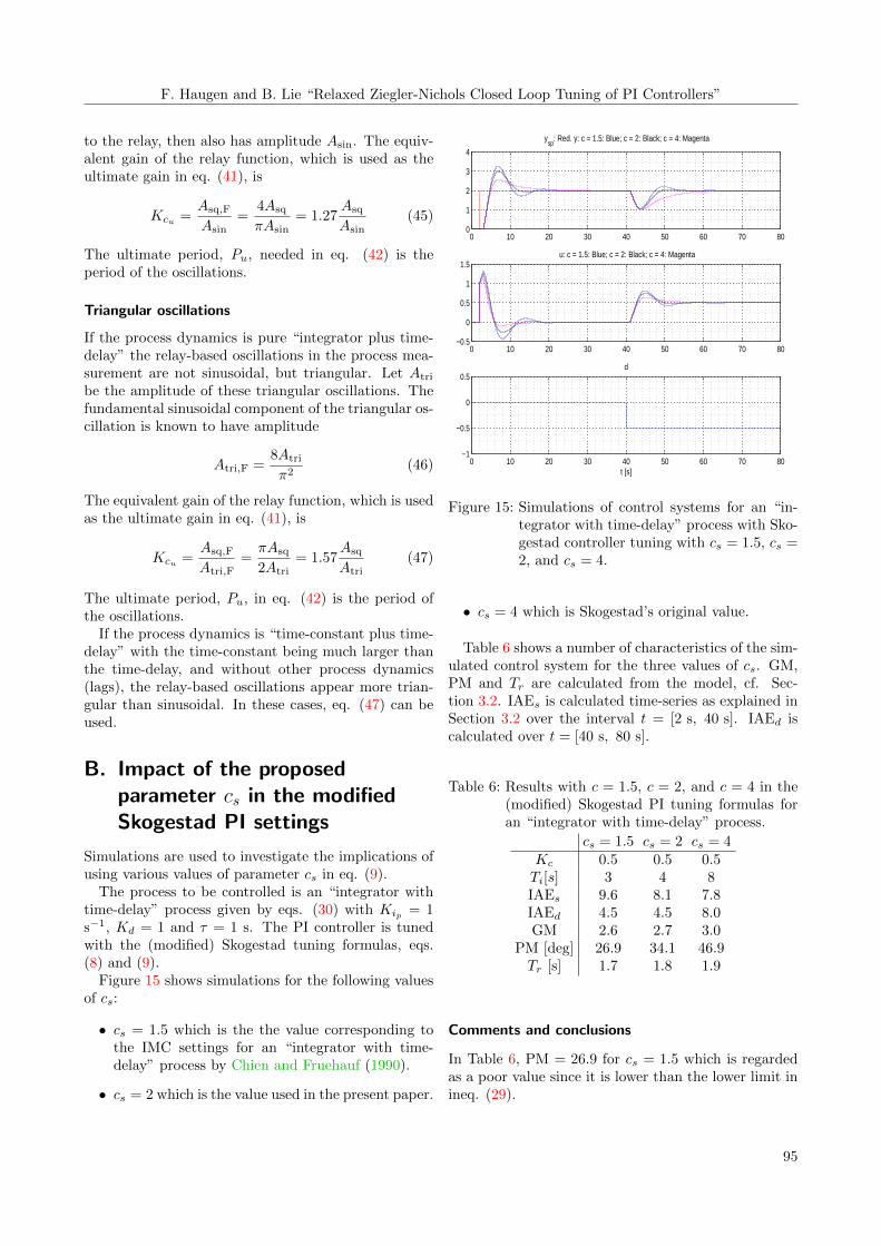
Figure 15 shows simulations for the following valuesof cs:

• cs = 1.5 which is the the value corresponding tothe IMC settings for an “integrator with time-delay” process by Chien and Fruehauf (1990).

• cs = 2 which is the value used in the present paper.

0 10 20 30 40 50 60 70 800

1

2

3

4

ysp

: Red. y: c = 1.5: Blue; c = 2: Black; c = 4: Magenta

0 10 20 30 40 50 60 70 80−0.5

0

0.5

1

1.5u: c = 1.5: Blue; c = 2: Black; c = 4: Magenta

0 10 20 30 40 50 60 70 80−1

−0.5

0

0.5d

t [s]

Figure 15: Simulations of control systems for an “in-tegrator with time-delay” process with Sko-gestad controller tuning with cs = 1.5, cs =2, and cs = 4.

• cs = 4 which is Skogestad’s original value.

Table 6 shows a number of characteristics of the sim-ulated control system for the three values of cs. GM,PM and Tr are calculated from the model, cf. Sec-tion 3.2. IAEs is calculated time-series as explained inSection 3.2 over the interval t = [2 s, 40 s]. IAEd iscalculated over t = [40 s, 80 s].

Table 6: Results with c = 1.5, c = 2, and c = 4 in the(modified) Skogestad PI tuning formulas foran “integrator with time-delay” process.

cs = 1.5 cs = 2 cs = 4Kc 0.5 0.5 0.5Ti[s] 3 4 8IAEs 9.6 8.1 7.8IAEd 4.5 4.5 8.0GM 2.6 2.7 3.0

PM [deg] 26.9 34.1 46.9Tr [s] 1.7 1.8 1.9


In Table 6, PM = 26.9 for cs = 1.5 which is regardedas a poor value since it is lower than the lower limit inineq. (29).

95


With cs = 2 and cs = 4 the stability margins areacceptable.

IAEd with cs = 2 is 56% of IAEd with cs = 4, in-dicating a considerable improved disturbance compen-sation with cs = 2. This is also clearly seen in thesimulations.

We prefer cs = 2 over cs = 4 in the Skogestad PIsettings formulas for “integrator plus time-delay” pro-cesses since the disturbance compensation is improved.

C. Abbreviations and nomenclature

C.1. Abbreviations

GM: Gain margin.

IAE: Integral of absolute error.

PI: Proportional plus integral (control).

PM: Phase margin.

R-ZN: Relaxed Ziegler-Nichols.

ZN: Ziegler-Nichols (original method).

TL: Tyreus-Luyben.

SIMC: Simple Internal Model Control.

C.2. Nomenclature

Asin: Amplitude of sinusoidal wave in control error orin process (output) measurement.

Asq: Amplitude of square wave in control signal.

Atri: Amplitude of triangular wave in control error orin process (output) measurement.

Au: Amplitude of the on-off control signal.

cs: Parameter introduced in the integral time settingsin the Skogestad method.

d is process disturbance.

∆: Deviation from operating point.

e: Control error. e = ysp − y.

kr: The relaxation parameter in the Relaxed Ziegler-Nichols method.

K is process gain.

Kc [s]: Controller proportional gain.

Kd is disturbance gain.

Kip [s]: Process integrator gain.

Pu [s]: Period of sustained oscillations.

T [s]: Process time-constant.

Tc [s]: Closed loop time-constant.

Ti [s]: Controller integral time.

Tr [s]: Response-time, or 63% rise time of step re-sponse.

τ [s]: Process time-delay.

u: Control signal (controller output).

uman: Manual control signal (control bias).

y: Process output measurement.

ysp: Setpoint

References

Astrøm, K. J. and Hagglund, T. PID Controllers: The-ory, Design and Tuning. ISA, 1995.

Chien, I. L. and Fruehauf, P. S. Consider IMC Tun-ing to Improve Controller Performance. Chem. Eng.Progress, 1990. Oct:33–41.

DiRuscio, D. On Tuning PI Controllers for In-tegrating Plus Time Delay Systems. Modeling,Identification and Control, 2010. 31(4):145–164.doi:10.4173/mic.2010.4.3.

Haugen, F. The good gain method for simple ex-perimental tuning of pi controllers. Modeling,Identification and Control, 2012. 33(4):141–152.doi:10.4173/mic.2012.4.3.

Haugen, F. Air heater. http://home.hit.no/~finnh/air_heater, 2013.

Haugen, F., Bakke, R., and Lie, B. Temperature con-trol of a pilot anaerobic digestion reactor. Submittedto Modeling, Identification and Control, 2013.

Haugen, F. and Lie, B. On-off and pid control ofmethane gas production of a pilot anaerobic diges-tion reactor. Submitted to Modeling, Identificationand Control, 2013.

Seborg, D. E., Edgar, T. F., and Mellichamp, D. A.Process Dynamics and Control. John Wiley andSons, 2004.

96



http://home.hit.no/~finnh/air_heater

http://home.hit.no/~finnh/air_heater


Skogestad, S. Simple analytic rules for model re-duction and pid controller tuning. Modeling,Identification and Control, 2004. 25(2):85–120.doi:10.4173/mic.2004.2.2.

Tyreus, B. D. and Luyben, W. L. Tuning PI Con-trollers for Integrator/Dead Time Processes. Ind.Eng. Chem, 1992. 31(31).

Yu, C. C. Autotuning of PID Controllers. SpringerVerlag, 1999.

Ziegler, J. and Nichols, N. Optimum settings for au-tomatic controllers. Trans. ASME, 1942. 64(3):759–768. doi:10.1115/1.2899060.

97


http://dx.doi.org/10.1115/1.2899060

http://creativecommons.org/licenses/by/3.0

relaxed ziegler-nichols closed loop tuning of pi … · modeling, identi cation and control, vol....

Documents