reit stock price volatility during the financial crisis · reit stock price volatility during the...

REIT Stock Price Volatility during the Financial Crisis

Yuichiro KawaguchiΨ J. Sa-Aadu† James D. Shilling‡

Waseda University University of Iowa DePaul University

Revised Draft December 2012

Abstract

This paper sheds light on several puzzling empirical observations. We examine thevolatility implications of equity REIT stock returns over the sample period from Jan-uary 1985 through October 2012. We find a negative “leverage effect” in the pre- andpost-Greenspan era, but not during the Greenspan era (circa 1994 to 2006). We arguethat the positive elasticity of variance with respect to the value of equity during theGreenspan era can be explained by low and declining interest rates, which triggered awealth transfer from REIT equity holders to REIT debt holders. We also argue thatthe low and declining interest rates during the Greenspan era allowed REITs to take onfar more risk than most people realized. We then document that average REIT stockreturn volatility increased significantly in the 2007-2010 period in the midst of a historicdecline in REIT stock prices. The results have significant implications for the good dealof interest and debate in the media over the status of REITs and whether equity REITshave become excessively risky relative to the returns they generate.

Keywords: REIT Liquidity, Trading Volume, Asset Pricing

JEL Classification: G0, G1, G12

ΨWaseda University, Graduate School of Finance, Accounting & Law 1-4-1 NihombashiChuo-ku, Tokyo, Japan 103-0027, Email: [email protected].†University of Iowa, Department of Finance, Suite 252, Iowa City, IA 52242, Email: [email protected].‡DePaul University, 1 East Jackson Boulevard, Chicago, IL 60604, Email: [email protected].

1. Introduction

The recent increase of average REIT stock return volatility in the 2007-2010 period (see

Figure 1, which shows the standard deviation of the total monthly return on the equity

National Association of Real Estate Investment Trust (NAREIT) index) is not as puzzling

as it appears at first glance. A large part of the increase (as we shall argue below) can be

explained by a long period of low and declining interest rates in the Greenspan era (circa

1994 to 2006). The low interest rates of that period triggered a wealth transfer from REIT

equity holders to REIT debt holders and raised the financial leverage ratio of REITs (defined

as the market, rather than the face, value of debt divided by the market value of equity).

At the same time, the ratio of the total face value of debt divided by the market value of

equity declined, leaving most REITs headroom (as long as business and financial risk did

not materialize) to take on more (relatively cheap) debt to push their yields even higher.

Financed with a capital structure with heavier amounts of (albeit relatively low-cost) debt,

REITs harbored far more risk than most people realized. At this juncture, the developments

in the financial crisis of 2007-2009 (i.e., increased business and financial risk) led to declining

stock prices. As stock prices fell, other things equal, the market financial leverage ratio and

equity volatility for REITs increased.1

The balance sheets of REITs are very susceptible to external shocks. This vulnerability is

not a new situation. It has been something REITs have had to deal with on a regular basis.

It is caused by REITs’ inability to retain significant amounts of cash flow. REITs are also

more dependent on short-term liquidity sources than companies in other sectors because of

1Other literature about REIT volatility suggests that leveraged or inverse-exchange traded funds (ETFs)have exacerbated intraday REIT volatility. See Bond and Hatch (2011), and Boney and Sirmans (2008). Butleveraged or inverse-ETFs alone cannot explain the increase of average REIT stock return volatility over the2007-2010 period.

1

their inability to retain significant amounts of cash flow. REITs typically utilize short-term

liquidity sources to acquire properties and fund certain development and capital expenditures.

Thus, during periods of liquidity stress in the capital markets REITs can be subject to a rather

large leverage effect intertemporally.

A simple test of this theory presents itself. These events make clear that the relation

between changes in equity value and equity volatility for levered REITs may at times be

positive or negative. Indeed, before and after the Greenspan era, when REIT stock prices were

increasing, we would have expected a negative relation between equity value and volatility.

However, during the Greenspan era, we would have expected the relation between the variance

of equity returns and REIT stock price to be positive. As explained by Black (1976), the

former is consistent with classical contingent claims theory made in Merton (1974). The

latter is consistent with the argument made in Christie (1982) and elsewhere. The latter is

also consistent with evidence that, on average, stocks react negatively to both the interest

rate (expected inflation) and unexpected inflation.

The results reported here have important implications. The financial press often compares

investing in REIT stocks to investing in fixed-income bonds. However, in today’s environment

reports have begun to appear that with the high yield on REIT stocks also comes a high

degree of risk, and that this high degree of risk makes REIT stocks an extremely volatile

investment alternative to (lower yielding/lower risk) fixed income and/or treasury products

(see, e.g., Campbell (2011) writing in U.S. News & World Report). This assertion overlooks

two important factors. First, that REITs have delevered notably since 2007. Holding firm

volatility constant, a decrease in the ratio of the total face value of debt divided by the

market value of equity implies a decrease in equity volatility. Second, REITs have enjoyed

2

a large increase (i.e., rebound) in stock values since 2007. With a negative variance/stock

price relation, the price effect implies (if our empirical results as reported below are valid) a

decrease, rather than an increase, in REIT equity volatility.

Testing for a negative/positive relation between volatility and the value of equity for

REITs occupies the remainder of the paper. The next section quickly reviews the contingent

claims literature on the links between equity volatility and equity value. The third section

reviews the literature on the relationship of equity volatility and equity value caused by an

increase/decrease in interest rates. The model provides motivation for the empirical tests.

The fourth section describes the data used in the analysis. The fifth section presents tests of

trade-off between equity volatility and equity value for all equity REIT stocks that comprise

the FTSE National Association of Real Estate Investment Trust (NAREIT) Equity REIT

index. Separate tests are presented to examine the sensitivity of the results to different

subperiods. We find a negative REIT stock price elasticity of variance before and after the

Greenspan era, but not during the Greenspan era. The sixth section reports some additional

checks of robustness. The checks serve to validate the core findings. The concluding section

summarizes the main findings of the paper. The results are significantly different from those

given by Schwert (1989, 2010).

2. Merton’s Model of Equity Volatility

2.1 Contingent Claims Theory

Merton (1974) presents a model of equity and debt valuation in which financial markets are

assumed to be perfect. The model assumes that a firm with initial value V issues a zero-

coupon bond with face value D and maturity T . Firm value is assumed to be lognormally

3

distributed and trading is continuous. Interest rates, the payout rate, and volatility are all

assumed constant. The firm is assumed to follow a pattern of rational default. That is, default

occurs at the maturity of the discount debt if V < D, which means that equity is an option

on firm value that pays Max(V −D, 0) at time T .

Under the condition of risk-free debt and costless bankruptcy, the Black and Scholes (1973)

formula gives the value of equity of the firm, S. Here S increases with 1) an increase in value

of the firm’s assets, V , 2) an increase in the variance of the value of the firm’s assets, and

3) an increase in the time to maturity of the amount of debt D. The value of the debt, D,

is equal to firm value minus the value of equity. With respect to the value of the firm, firm

value is completely independent of the type of financing used for its projects. That is, the

Modigliani-Miller proposition of leverage irrelevance holds.

The upshot of Merton’s model is that for a given firm

σS = (V SV /S) × σV (1)

where σ denotes the standard deviation of the rate of return, SV is the derivative of equity

value with respect to firm value (i.e., the call option’s delta), and V and S represent the

market values of the firm and equity respectively. Options delta values range from 0 to 1.

Options delta values rise as options get more and more in-the-money and reduce as the options

get more and more out-of-the-money. With SV = 1, (1) reduces to

σS = (1 + LR) × σV (2)

where LR = D/S is the market financial ratio. Equation (2) makes clear that as the value

4

of equity increases, the firm becomes less levered and as a result the volatility of equity falls.

That is, there is a negative relation between equity volatility, σS , and the value of equity, S.

The negative relation between equity volatility and the value of equity is also implied in the

Cox and Ross (1976) model of equity and debt valuation.

2.2 Empirical Implementation

Beckers (1980) is an example of an attempt to test the link between equity volatility and the

value of equity in the Cox and Ross (1976) model. For example, for ordinary stocks Beckers

(1980) reports a regression of the form:

lnσS = κ0 + κ1lnS + ε (3)

where ε is a random error term. The value of κ1 in this model should vary from −1 to 0.

Hence, equity volatility is an inverse function of stock price.

Christie (1982) performs related tests, in that he estimates

ln(σS/σS−1

) = β0 + β1ln(S/S−1) + µ (4)

Christie’s (1982) regression model can be derived from (2) by assuming that the elasticity of

equity volatility with respect to stock price is an intertemporal constant, and then by adding

an intercept, β0, and an error term, µ. Empirically, one should expect the slope term, β1, to

be between -1 and 0 (ignoring estimation error and econometric problems).

Cheung and Ng (1987), Ritchken and Trevor (1999) and others propose a EGARCH

formulation for estimating the inverse relation between stock price and equity volatility, which

5

has the desirable property that stock returns are function of conditional volatility. The model

can be written as

r = a+ bh+ cr−1 + u (5)

lnh = α+ γ lnh−1 +

2∑

j=1

λjz−j + θlnS−1 (6)

where

u ∼ N(0, h)

z−k = [|ψ−k| − (2/π)0.5 + ηψ−k]

u−k = ψ−k

√

h−k

ψ ∼ i.i.d.N(0, 1)

r is the rate of return on equity and h is the variance of the error term, u, conditioned on

information available at time t− 1. The conditional variance is a function of four terms: the

constant, α, the ARCH terms, z−k, the GARCH term, lnh−1, and the log stock price, lnS−1.

The ARCH term tests for whether volatility propagates over time (i.e., whether a volatility

shock from prior periods leads to an increased volatility today). The GARCH term captures

whether large volatility shocks cause a large and persistent increase in volatility.2 The log

stock price is incorporated in (6) to test whether equity returns become more volatile as stock

prices decrease. In (5), the value of b should be positive. That is, returns should be higher

during times of higher volatility. In (6), to model persistence of higher volatility, one needs a

process with positive values for γ and λk. Lastly, in (6) the coefficient θ should be negative.

2Using the GARCH model given can be justified by appealing to the recent work by Case, Guidolin andYildirim (2011), who find evidence of conditional heteroskedasticity in REIT returns.

6

That is, returns should become more volatility as prices decrease. One of the attractiveness

of the relations in (5) and (6) is that it captures the asymmetric effect of lagged shocks on

conditional volatility.

In the empirical section that follows, we shall estimate equations (3), (4), and (5)-(6), and

contrast the results. We shall be interested in knowing whether REIT equity returns become

more volatile as stock prices decrease, and whether a negative relation between REIT stock

price and equity volatility is a standard result. We shall also be interested in knowing the

effect of an increase/decrease in interest rates on the variance of REIT equity returns. It is

possible for REIT equity returns to become more volatile when interest rates fall. So the net

effect of an increase in REIT stock prices and a decrease in interest rates could lead to an

increase, rather than a decrease, in the REIT equity volatility, depending on which effect is

stronger. We turn to this issue next.

3. The Effect of Changing Interest Rates

Christie (1982) documents that increases (decreases) in interest rates can have a negative (pos-

itive) impact on the volatility of equity. This result can be shown by differentiating equation

(1) directly with respect to the interest rate, r, and evaluating the obtained expression:

∂σS/∂r = σV S−1 {VrεSSV λS + (V SV r − εSSr)} (7)

where SV is the partial derivative of S with respect to V , Sr is the partial derivative of S

with respect to r, SV r is the cross partial of S with respect to V and r, Vr is the partial

derivative of V with respect to r, εS is the elasticity of the value of equity with respect to

value of the firm (i.e., εS = V SV /S), and λS is the elasticity of equity volatility with respect

7

to stock price (i.e., λS = (∂σs/σS)/(∂S/S)).

Since SV r is negative–an increase in V has less impact on S in a high interest rate environ-

ment compared with a low interest rate environment – and Sr is positive – an increase in inter-

est rates makes the equity holder better off, holding all else constant – the term (V SV r−εSSr)

must be negative, given εS is positive. The term VrεSSV λS is positive provided λS is negative

and Vr < 0. In this case, ∂σS/∂r is positive if VrεSSV λS > (εSSr−V SV r), that is, an increase

in interest rates could lead to an increase in volatility where VrεSSV λS > (εSSr) − V SV r).

Alternatively, if λS is positive (as in the case where Vr = 0), ∂σS/∂r can be negative, and the

model has an interesting interpretation. It says that a decline in interest rates (like what took

place during the Greenspan era) could lead to a positive association between equity variances

and equity value. The intuition is simple enough. A decline in interest rates causes the value

of debt and equity both to increase but the debt increases more than the equity. As debt

values increase more than the equity, the financial leverage of the firm increases. Because of

the positive association between equity variances and financial leverage, the increase in finan-

cial leverage leads to an increase in the volatility of the stock, creating a positive relationship

between equity variances and equity value that is not fabricated or trumped-up.

Whether declining interest rates during the Greenspan era led to a positive elasticity

between REIT equity volatility and stock price is an integral part of our story and is analyzed

below. We shall first conduct a test for all REIT stocks in the 1985-1993 period to examine the

relation between REIT stock price and equity volatility. Next, we will undertake robustness

test by examining the sensitivity of the results to different subperiods. Empirically, one should

expect to observe a positive elasticity of REIT equity volatility with respect to the stock price

during the Greenspan era and a negative elasticity of REIT equity volatility with respect

8

to the stock price in all other subperiods. Again, we will estimate the models described in

equations (3), (4), and (5)-(6), and contrast the results.

4. Data

The basic data consist of monthly returns for all equity REIT stocks of NYSE, AMEX,

and NASDAQ-listed companies that comprise the FTSE NAREIT Equity REIT index. The

sample period runs from January 1985 through October 2012. We estimate the model first

for the subsample period from January 1985 through December 1993 – the pre-Greenspan

era – and then from January 1994 through December 2006 – the Greenspan era – and from

January 2007 through October 2012 – the post-Greenspan era. The sample is split into these

three subsample periods to see if parameters changed in the Greenspan era for the reasons

mentioned above.3

Using an index made up of all equity REIT stocks to test the hypothesis that the elasticity

of REIT equity volatility with respect to the value of equity is negative is somewhat objection-

able because the elasticity of leverage may vary with a number of other factors. For example,

the propensity for REIT equity volatility to increase with respect to a fall in stock price may

vary nonlinearly with operating leverage (i.e., fixed costs) and the revenue (state) generating

process. Specifically, it is possible for a small decrease in stock price to have a larger impact

on equity volatility if the REIT has a high degree of operating leverage compared to a REIT

with a low degree of operating leverage. It is also possible for the behavior of REIT equity

3The break in the sample period in January 1994 is roughly consistent with the first full year of what mightbe considered the modern REIT era. It is possible that the interest rate level played a role in stimulatingthe modern-side of REITs. Modern REITs are generally distinguished from their predecessors by a numberof financial features, including owning higher-quality assets and adopting a more leveraged risk profile. Thereis a substantial body of literature that explains when financial innovations occur. The evidence on financialinnovations points to the conclusion that new innovations largely stem from an increase in the cost of adheringto existing constraints; for example, the rising costs of adhering to existing financing constraints (see, e.g.,Silber (1983)). This perspective can be used to explain the steady change in REIT investing and the adoptionof a more leveraged risk profile.

9

volatility to vary with growth and redevelopment opportunities. Everything else equal, RE-

ITs with significant growth and redevelopment opportunities should have greater risk (risk

and opportunity are two sides of the same coin). Consequently, the elasticity of REIT equity

volatility with respect to the value of equity may vary nonlinearly with growth opportunities.

Another variable that can impact volatility is firm size. Chan and Chen (1988) and others

find that firm size helps to explain the cross-section of average stock returns. Firms with low

market equity are more likely to have poor prospect, whereas large stocks are more likely to

be firms with stronger prospects. What this suggests is that firm size may have an effect

on the relation between equity volatility and financial leverage. Anticipating this, separate

equity volatility and stock price indices were prepared for the different groups of REITs.4

The underlying data used to construct these indices are from the COMPUSTAT files of

income-statement and balance-sheet data. The indices are constructed by taking fiscal year-

end fundamental data in calendar year t−1 for constituents of the NAREIT index to compute

their operating leverage and earnings growth rate. There are several ways to measure earnings

growth. We measure earnings growth (defining earnings as earnings before interest, taxes,

depreciation and amortization) for each firm as

ECit = 100 × [Eit − Eit−1] /|Eit−1| (8)

where ECit is the earnings change for the ith firm in the tth period and Eit is earnings per

share for the ith firm in the tth period. The use of the absolute value of earnings in the

denominator is to correct for negative and positive earnings numbers. The analysis truncates

outliers at ±100%. This truncation essentially precludes any one observation from dominating

4A separate argument for focusing attention on large REITs appears in Cotter and Stevenson (2008). Theysuggest that the inclusion of REITs in large indices has increased fund flows into the industry and increaseddaily REIT volatility.

10

the averages. We measure operating leverage for each firm as

DOLit = 100 ×

{[

Eit −Eit−1

|Eit−1|

]

/

[

Rit − Rit−1

Rit−1

]}

(9)

where DOLit is the degree of operating leverage for the ith firm in the tth period and Rit is

total revenues for the ith firm in the tth period. We use a firm’s market equity at the end of

December of year t− 1 to compute its market size (stock price times shares outstanding).

In December of each year, all firms are separately sorted by operating leverage, earnings

growth rate, and size to determine mean breakpoint values for each grouping. Firms are then

allocated to two size portfolios – high and low – based on these breakpoints. After assigning

firms to these (non-mutually exclusive) portfolios in December, we calculate equal-weighted

monthly returns on the portfolios for the next 12 months, from December to December. In

the end, we have monthly returns for REITs with high and low operating leverage alone, high

and low earnings growth rates alone, and for both large and small REITs alone from January

1985 through October 2012. We use these indices to test whether the elasticity of financial

leverage varies with operating leverage, earnings growth, and size.

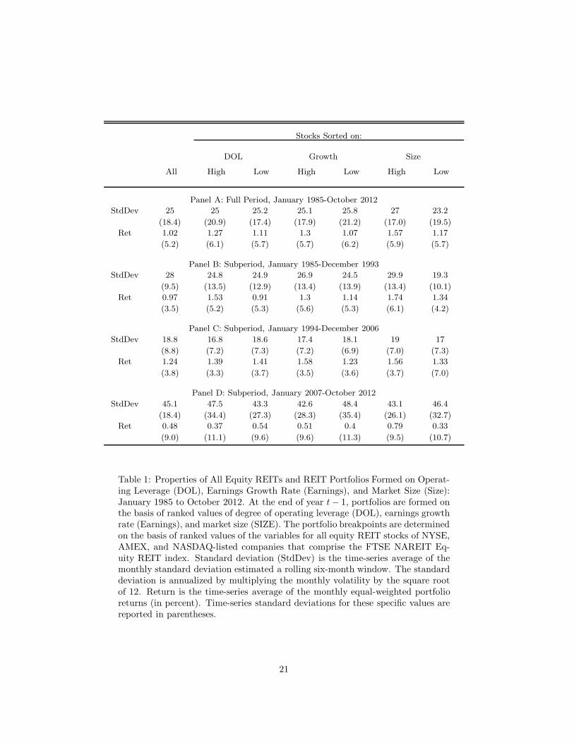
Table 1 reports standard deviations and mean returns for the full period as well as for the

three different subperiods for the indices described above. The standard deviation is measured

in nominal terms using a rolling six-month window.5 The standard deviation is annualized

by multiplying the monthly volatility by the square root of 12. Over 1985 to 2012, all equity

REITs displayed returns of 1.02 percent (or at a rate of 13 percent compounded annually).

Higher returns are observed over the 1994-2006 Greenspan era. For instance, all equity REITs

5There is evidence in Chung, Fung, Shilling, and Simmons-Mosley (2011), and Diavatopoulos, Fodor,Howton, and Howton (2010) that implied volatility from the REIT option market is generally a good, but nota perfect, estimator of realized volatility in the REIT stock market and vice versa.

11

displayed returns of 1.24 percent (or 15.9 percent compounded annually) over the period 1994

to 2006. Higher returns are also observed for REITs with high operating leverage compared

to REITs with low operating leverage, REITs with high earnings growth compared to REITs

with low earnings growth, and large-size REITs compared to small-size REITs. The table also

shows that highest standard deviations are observed over more recent periods. For example,

all equity REITs experienced an average standard deviation of 45 percent over the period 2007

to 2012 (compared to 28 percent over the period 1985 to 1993). Additionally, REITs with

high operating leverage and low earnings growth rate as well as small-size REITs grappled

with high standard deviations over the period 2007 to 2012.

As Figure 2 shows, the ratio of debt-to-EBITDA for REITs in the U.S. increased sharply

over the 1994-2006 Greenspan era, from 3.7 times EBITDA in 1994 to 6.7 times EBITDA

in 2007. Figure 2 also highlights the precipitous downward trend of debt-to-EBITDA in the

post-2009, from 8.8 times EBITDA in 2009 to 6.8 times EBITDA in 2012. The trend toward

a declining debt-to-EBITDA ratio is consistent with an increasing equity-to-total-asset ratio,

increasing from 36 percent in 2009 to 43 percent. The trend is also consistent with more rapid

NOI growth in 2009-2012, rates of increase between 9.5 percent and 21.8 percent.6

5. Tests of the Financial Leverage Hypothesis

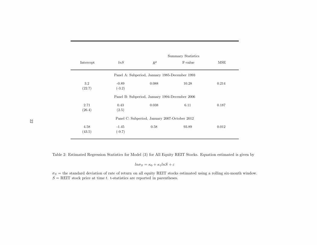
Estimates of models (3), (4), and (5)-(6) for all equity REIT stocks are obtained for each

period. The results are presented in Tables 2-4. Table 2 presents the results of the estimations

of model (3). Several interesting observations emerge from Table 2. First, we find an inverse

relation between REIT stock price and volatility for the subsample period from January

6All of these financial ratios are for all US-equity REITs and come from SNL’s REIT database, whichprovides detailed firm classification and financial information of REITs.

12

1985 through December 1993 and from January 2007 through October 2012, but not over the

Greenspan era from January 1994 to December 2006. The estimate of the price variable in the

subsample period from January 1985 to December 1993 is -0.89 and statistically significant

at conventional levels. A plot of the standard deviation of REIT stock prices against the

logarithm of stock price from January 1985 to December 1993 is given in Figure 3. The plot

confirms a negative downward trend. The estimate of the price variable in the January 1994

to December 2006 period is 0.43, with a t-statistic of 2.5 (significant at the 5 percent level). A

plot of the standard deviation of REIT stock prices against the logarithm of stock price from

January 1994 to December 2006 is given in Figure 4. The plot confirms an upward positive

trend. The estimate of the price variable in the subsample period from January 2007 through

October 2012 is -1.45, with a t-statistic of -9.7 (significant at the 1 percent level). A plot of the

standard deviation of REIT stock prices against the logarithm of stock price from January

2007 through October 2012 is given in Figure 5. The plot confirms a negative downward

trend. So in the pre- and post-Greenspan era, the lower are REIT stock prices, the higher is

REIT volatility. However, in the Greenspan era, the higher are REIT stock prices, the higher

is REIT volatility. Second, estimates of the leverage effect in the pre- and post-Greenspan

era are generally consistent with Beckers (1980), Christie (1982), and French, Schwert, and

Stambaugh (1987), who estimate an average cross-sectional stock price elasticity of variance

for ordinary firms to be between -0.40 and -3.38. Third, the results are contrary to Schwert

(1989), who finds that leverage had a relatively small effect on stock volatility during the

1929-1940 Great Depression. In contrast, in a similar analysis of stock volatility during the

recent financial crisis, Schwert (2010) shows that the volatility of stock prices, particularly

among financial sector stocks, was on the whole linked with real economic activity.

13

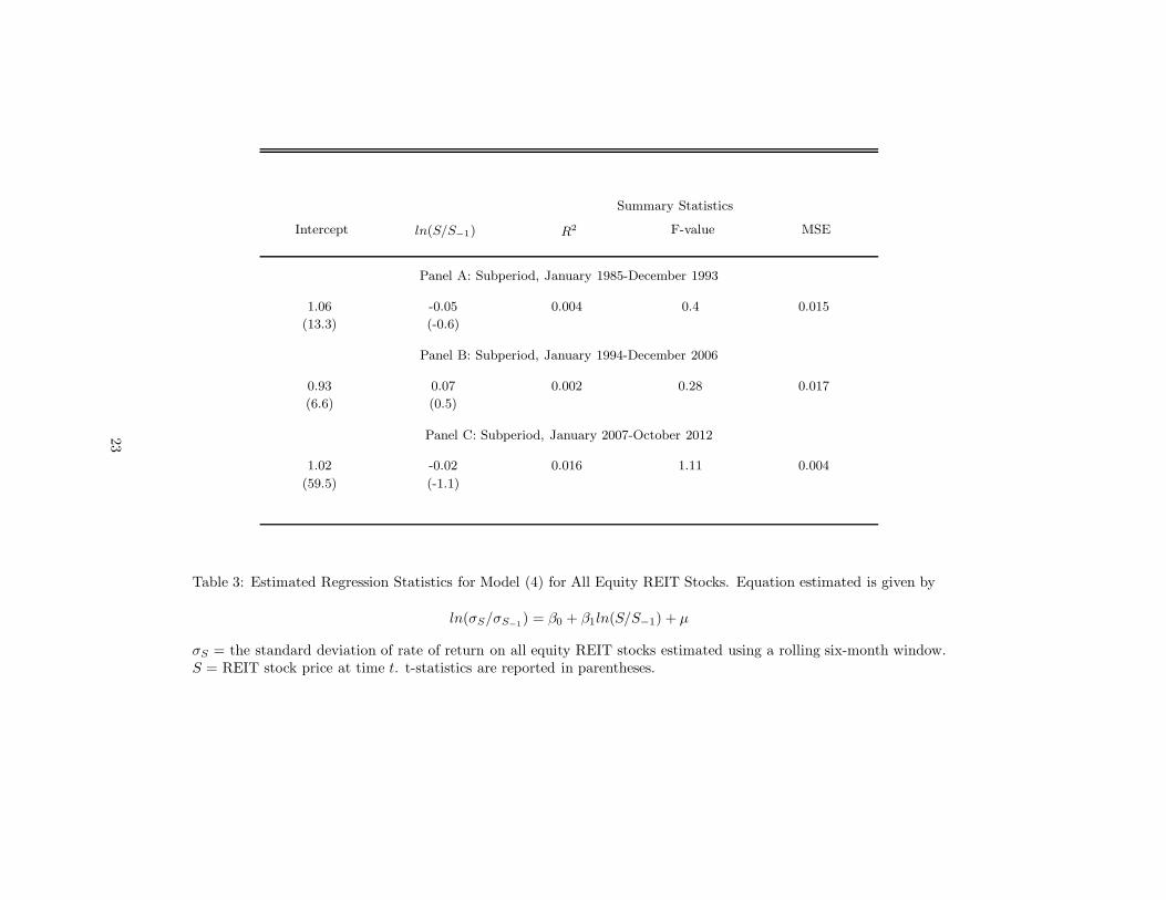
Table 3 presents the results of the estimations of model (4). The coefficient of the price

ratio variable indicates the leverage effect on REIT volatility. In the pre- and post-Greenspan

era, the coefficient of the price ratio variable is negative but not significant. In the Greenspan

era, the coefficient of the price ratio variable turns positive but not significant. The statistical

problem is that the independent variable varies across time but the dependent variable, a ratio

of standard deviations, does not. While this inability to associate variation in the dependent

variable with the independent variable leads to less precise estimates, it does not change the

basic story.

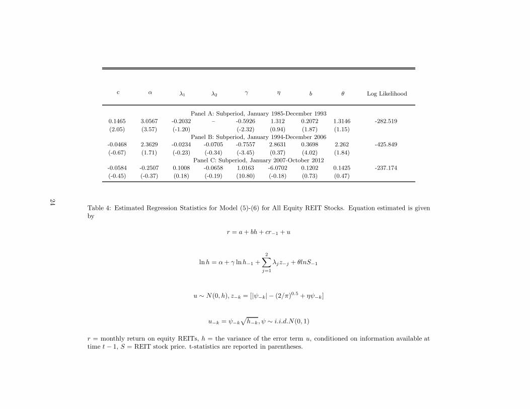
Table 4 presents the results of the estimation of model (5)-(6). Several points are worth

noting. First, the regressions serve as a benchmark to document that over the January 1994

to December 2006 period REIT volatility did exhibit a positive relation with stock price.

The REIT stock price elasticity of variance in the Greenspan era is 2.26, with a t-statistic

of 1.84. The results are consistent with the evidence of a positive relation between REIT

volatility and stock price in the January 1994 to December 2006 period found in Tables 2

and 3. Second, given that the sign of λ1 in the January 2007 to October 2012 period is

positive, the negative sign of η implies that unexpected negative REIT stock returns have

a larger impact on future conditional stock volatility than unexpected positive REIT stock

returns. This evidence indicates that the developments during the financial crisis which led

to declining REIT stock prices also led to increased REIT volatility. Third, the stock price

elasticity of variance in the pre- and post-Greenspan era are insignificant. The results are

consistent with a nonlinear relationship between REIT stock price and its variance.

14

6. Robustness Tests

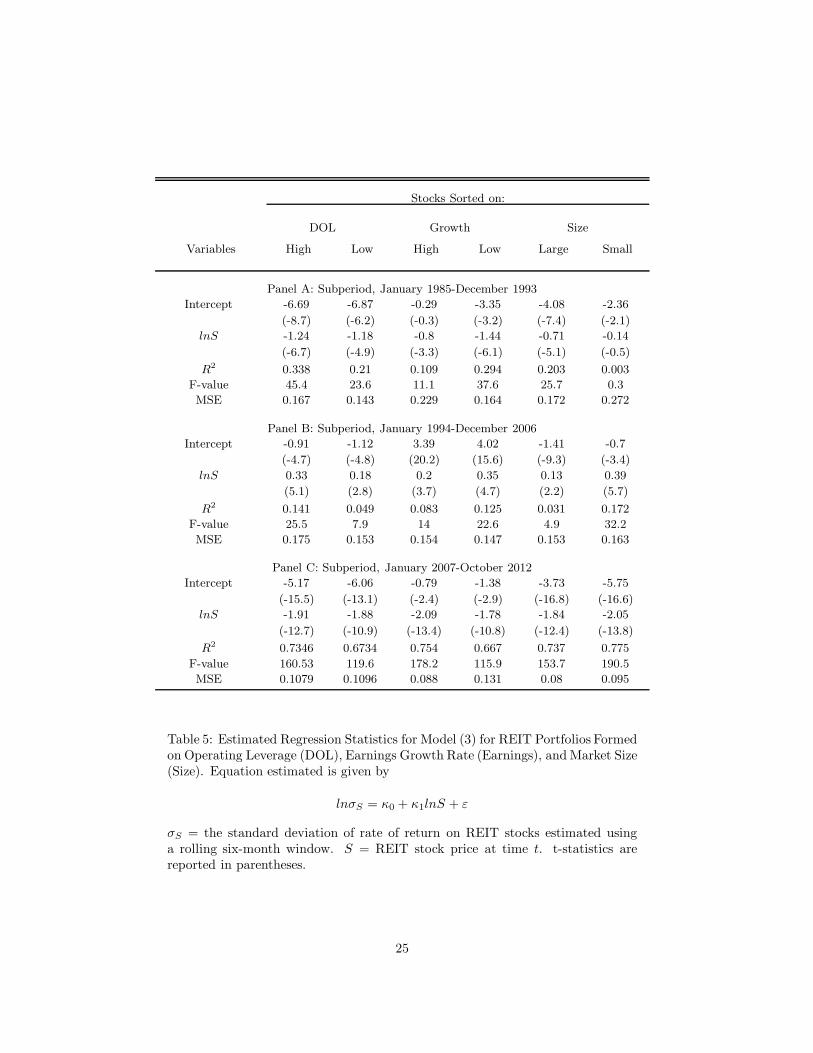
In this section we present a series of robustness checks. First, it is possible that operating

leverage may impact equity volatility and thereby influence or obscure the hypothesized rela-

tionship between equity volatility and the value of equity. We simplified (3) by estimating it

for REITs with high versus low operating leverage. See Table 5, columns (1) and (2). Similar

results to Table 2 were obtained, as again we find an inverse relation between REIT stock

price and volatility for REITs with both high and low operating leverage for the subsample

periods from January 1985 through December 1993 and from January 2007 through October

2012, but not over the Greenspan era from January 1994 to December 2006. Again, the results

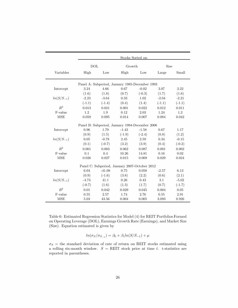
of the estimation of model (4) for REITs with both high and low operating leverage yields

less precise estimates, as can be seen by the t-values reported in Table 6, columns (1) and

(2). In addition, we find that our original results of estimating model (5)-(6) are unchanged

when the model is estimated for REITs with high versus low operating leverage. The average

REIT stock price elasticity of variance for REITs with both high and low operating leverage

implies that there is a positive and significant relationship between REIT stock volatility and

stock price over the subsample period January 1994 to December 2006. See Table 7, columns

(1) and (2).

The second issue is that earnings growth may impact equity volatility and through this

effect the parameter estimates obtained above could be biased and inconsistent. Thus, to

check on the robustness of our results, we re-estimated models (3), (4), and (5)-(6) for REITs

with high versus low earnings growth rates. Table 5, columns (3) and (4) present the results

of the estimations of model (3). The coefficients of the price variable for REITs with both

high and low earnings growth rates for the subsample periods from January 1985 to December

15

1993 and from January 2007 through October 2012 are negative and significant, but we again

find positive and significantly different from zero estimates for REITs with both high and low

earnings growth rates in the January 1994 to December 2006 period. Table 6, columns (3)

and (4) present the results of the estimations of model (4). The estimates for the subsample

periods from January 1985 to December 1993 and from January 2007 through October 2012

are imprecise, but the coefficients of the price ratio variable for the January 1994 to December

2006 period are positive and significantly difference from zero. Table 7, columns (3) and (4)

present the results of the estimations of model (5)-(6). We find that our original results are

unchanged. The average REIT stock price elasticity of variance for REITs with both high and

low earnings growth rates is positive and significantly different from zero over the subsample

period January 1994 to December 2006.

A third possibility is that equity volatility could be affected by market size. We partitioned

our sample of equity REITs into two groups – large versus small. We re-estimated models

(3), (4), and (5)-(6) for large versus small REITs to investigate this omitted variable bias. It

appears that there is a negative relation between REIT equity volatility and stock price for

both large and small REITs in the subsample periods from January 1985 through December

1993 and from January 2007 through October 2012, but not over the Greenspan era from

January 1994 to December 2006. See Table 5, columns (5) and (6). Again, the estimation

of (4) provides an ineffective means of testing the hypothesized relationship between equity

volatility and the value of equity. See Table 6, columns (5) and (6). Finally, when model

(5)-(6) is re-estimated for large versus small REITs, we find strong evidence of a positive and

statistically significant average REIT stock price elasticity of variance over the subsample

period January 1994 to December 2006, especially for large REITs. See Table 7, columns

16

(5) and (6). In summary, on the basis of this series of analyses to assess the robustness of

the financial leverage hypothesis for REITs, we can be more confident that the conclusions

regarding the relation between REIT equity volatility and stock price presented above are

correct.

7. Conclusions

Taken together, our findings strongly point to a negative REIT stock price elasticity of vari-

ance before and after the Greenspan era, but not during the Greenspan era (circa 1994 to

2006). This result is not as puzzling as it might at first appear. The reasoning turns on the

low and declining interest rates during the Greenspan era. As Christie (1982) and others have

argued, low and declining interest rates give arise to a wealth transfer from equity holders

to debt holders. This wealth transfer is reflected in the value increment of debt relative to

equity, which implies an increase in financial leverage. With a strong positive association

between equity variances and financial leverage, a positive relation between the variance of

equity returns and equity value is expected. The latter occurs because the value of the debt

and equity both increase as the interest rate falls but the debt increases more than the equity.

Such behavior changes when interest rates are rising or when interest rates are more volatile

and uncertain. In such circumstances, the effect of an increase in stock price on the volatility

of equity is unambiguously negative.

Above, we use these arguments to provide new insight into ongoing controversies surround-

ing the volatility of REIT stock returns. Simple descriptive statistics show that equity REITs

increased their financial leverage during the Greenspan era. Such an increase caused REITs

to harbor far more risk than most people realized. But over the 1994 to 2006 period, no one

17

would have expected a significant increase in business and financial risk, or anticipated that

REIT stock prices would collapse in late 2008 and early 2009. However, as stock prices fell,

equity REITs became more levered than at any other time in history and equity volatility

increased (which is what the theory would predict and which is consistent with what we find).

The results reported here are valuable in what they tell us about the future rather than

the past. A view prevalent in the financial press (particularly now, after the recent increase of

average REIT stock return volatility in the 2007-2010 period) is that with the higher yield on

REIT stocks also comes a much higher degree of risk than an investment in a lower-yielding,

fixed-income security, much too high to warrant putting any investment dollars there. This

argument applies especially to risk-averse investors and fixed-income managers looking to

invest in REITs to boost yield because of their high dividends. Two important factors are

overlooked in this assertion. The first is the fact that REITs have delevered notably since

2007. The second factor is that REIT stock prices have recovered significantly since hitting

a bottom in February 2009. With a negative relation between volatility and value of equity

(as suggested by our empirical results), the increase in REIT stock prices implies a decrease

in equity volatility. This latter result clarifies a serious and generalized misunderstanding in

the literature.

18

8. References

Beckers, S., (1980), The Constant Elasticity of Variance Model and Its Implications For Op-tion Pricing. Journal of Finance, 35, 661-673.

Black, F., (1976), Studies of Stock Price Volatility Changes. Proceedings of the 1976 Meetingsof the American Statistical Association, Business and Economic Statistics Division, 171-181.

Black, F. and M. Scholes, (1973), The Pricing of Options and Other Corporate Liabilities.Journal of Political Economy, 81, 637-654.

Bond, S. A. and B. C. Hatch, (2011), Did Leveraged ETFS Increase Intraday REIT VolatilityDuring the Crisis? University of Cincinnati Working Paper.

Boney, V. and G. S. Sirmans, (2008), REIT ETFs and Underlying REIT Volatility, WorkingPaper.

Campbell, K., (2011), Three High-Yielding Fixed-Income Investment, US News & World Re-port.

Case, B., M. Guidolin, and Y. Yildirim, (2010), Do We Need Non-Linear Models to PredictREIT Returns? Univariate and Multivariate Evidence from Density Forecasts, Working Pa-per.

Chan, K. C. and N.F. Chen, (1988), An Unconditional Asset-Pricing Test and the Role ofFirm Size as an Instrumental Variable for Risk, Journal of Finance 43, 309-325.

Cheung, Y.W. and L. K. Ng, (1992), Stock Price Dynamics and Firm Size: An EmpiricalInvestigation, Journal of Finance, 47, 5, 1985-1997.

Christie, A. A., (1982), The Stochastic Behavior of Common Stock Variances – Value, Lever-age, and Interest Rate Effects. Journal of Financial Economics 10, 407-432.

Chung, R., S. Fung, J. D. Shilling and T. X. Simmons-Mosley, (2011), A Fear Factor in Im-plied Volatility for REIT Stocks? Working Paper.

Cotter, J. and S. Stevenson, (2008), Modeling Long Memory in REITs, Real Estate Eco-nomics 36, 3, 533-554.

Cox, S. J. and S. Ross, (1976), The Valuation of Options for Alternative Stochastic Processes,Journal of Financial Economics 3, 145-166.

19

Diavatopoulos, D. A. Fodor, S. D. Howton, and S. W. Howton, (2010), The Predictive Powerof REIT Implied Volatility and Implied Idiosyncratic Volatility, Journal of Real Estate Port-folio Management 16, 1, 29-39.

French, K. R., G. W. Schwert, and R. F. Stambaugh, (1987), Expected Stock Returns andVolatility, Journal of Financial Economics 19, 1, 3-29.

Merton, R. C., (1974), On the Pricing of Corporate Debt: The Risk Structure of InterestRates, Journal of Finance 29, 449-470.

Ritchken, P. and R. Trevor, (1999), Pricing Options under Generalized GARCH and Stochas-tic Volatility Processes, Journal of Finance, 54, 1, 377-402.

Schwert, G. W., (1989), Why Does Stock Volatility Change Over Time?, Journal of Finance44, 1115-1154.

Schwert, G. W., (2010), Stock Volatility During the Recent Financial Crisis, NBER WorkingPaper No. 16976.

Silber, W.L., (1983), The Process of Financial Innovation. American Economic Review, 73,89-95.

20

Stocks Sorted on:

DOL Growth Size

All High Low High Low High Low

Panel A: Full Period, January 1985-October 2012

StdDev 25 25 25.2 25.1 25.8 27 23.2

(18.4) (20.9) (17.4) (17.9) (21.2) (17.0) (19.5)

Ret 1.02 1.27 1.11 1.3 1.07 1.57 1.17

(5.2) (6.1) (5.7) (5.7) (6.2) (5.9) (5.7)

Panel B: Subperiod, January 1985-December 1993

StdDev 28 24.8 24.9 26.9 24.5 29.9 19.3

(9.5) (13.5) (12.9) (13.4) (13.9) (13.4) (10.1)

Ret 0.97 1.53 0.91 1.3 1.14 1.74 1.34

(3.5) (5.2) (5.3) (5.6) (5.3) (6.1) (4.2)

Panel C: Subperiod, January 1994-December 2006

StdDev 18.8 16.8 18.6 17.4 18.1 19 17

(8.8) (7.2) (7.3) (7.2) (6.9) (7.0) (7.3)

Ret 1.24 1.39 1.41 1.58 1.23 1.56 1.33

(3.8) (3.3) (3.7) (3.5) (3.6) (3.7) (7.0)

Panel D: Subperiod, January 2007-October 2012

StdDev 45.1 47.5 43.3 42.6 48.4 43.1 46.4

(18.4) (34.4) (27.3) (28.3) (35.4) (26.1) (32.7)

Ret 0.48 0.37 0.54 0.51 0.4 0.79 0.33

(9.0) (11.1) (9.6) (9.6) (11.3) (9.5) (10.7)

Table 1: Properties of All Equity REITs and REIT Portfolios Formed on Operat-ing Leverage (DOL), Earnings Growth Rate (Earnings), and Market Size (Size):January 1985 to October 2012. At the end of year t− 1, portfolios are formed onthe basis of ranked values of degree of operating leverage (DOL), earnings growthrate (Earnings), and market size (SIZE). The portfolio breakpoints are determinedon the basis of ranked values of the variables for all equity REIT stocks of NYSE,AMEX, and NASDAQ-listed companies that comprise the FTSE NAREIT Eq-uity REIT index. Standard deviation (StdDev) is the time-series average of themonthly standard deviation estimated a rolling six-month window. The standarddeviation is annualized by multiplying the monthly volatility by the square rootof 12. Return is the time-series average of the monthly equal-weighted portfolioreturns (in percent). Time-series standard deviations for these specific values arereported in parentheses.

21

Summary Statistics

Intercept lnS R2 F-value MSE

Panel A: Subperiod, January 1985-December 1993

3.2 -0.89 0.088 10.28 0.214

(22.7) (-3.2)


2.71 0.43 0.038 6.11 0.187

(26.4) (2.5)

Panel C: Subperiod, January 2007-October 2012

4.58 -1.45 0.58 93.89 0.012

(43.5) (-9.7)

Table 2: Estimated Regression Statistics for Model (3) for All Equity REIT Stocks. Equation estimated is given by

lnσS = κ0 + κ1lnS + ε

σS = the standard deviation of rate of return on all equity REIT stocks estimated using a rolling six-month window.S = REIT stock price at time t. t-statistics are reported in parentheses.

22

Summary Statistics

Intercept ln(S/S−1) R2 F-value MSE


1.06 -0.05 0.004 0.4 0.015

(13.3) (-0.6)


0.93 0.07 0.002 0.28 0.017

(6.6) (0.5)


1.02 -0.02 0.016 1.11 0.004

(59.5) (-1.1)

Table 3: Estimated Regression Statistics for Model (4) for All Equity REIT Stocks. Equation estimated is given by

ln(σS/σS−1

) = β0 + β1ln(S/S−1) + µ

σS = the standard deviation of rate of return on all equity REIT stocks estimated using a rolling six-month window.S = REIT stock price at time t. t-statistics are reported in parentheses.

23

c α λ1 λ2γ η b θ Log Likelihood


0.1465 3.0567 -0.2032 – -0.5926 1.312 0.2072 1.3146 -282.519

(2.05) (3.57) (-1.20) (-2.32) (0.94) (1.87) (1.15)

Panel B: Subperiod, January 1994-December 2006-0.0468 2.3629 -0.0234 -0.0705 -0.7557 2.8631 0.3698 2.262 -425.849

(-0.67) (1.71) (-0.23) (-0.34) (-3.45) (0.37) (4.02) (1.84)


-0.0584 -0.2507 0.1008 -0.0658 1.0163 -6.0702 0.1202 0.1425 -237.174

(-0.45) (-0.37) (0.18) (-0.19) (10.80) (-0.18) (0.73) (0.47)

Table 4: Estimated Regression Statistics for Model (5)-(6) for All Equity REIT Stocks. Equation estimated is givenby

r = a+ bh+ cr−1 + u

lnh = α+ γ lnh−1 +2

∑

j=1

λjz−j + θlnS−1

u ∼ N(0, h), z−k = [|ψ−k| − (2/π)0.5 + ηψ−k]

u−k = ψ−k

√

h−k, ψ ∼ i.i.d.N(0, 1)

r = monthly return on equity REITs, h = the variance of the error term u, conditioned on information available attime t − 1, S = REIT stock price. t-statistics are reported in parentheses.

24

Stocks Sorted on:

DOL Growth Size

Variables High Low High Low Large Small


Intercept -6.69 -6.87 -0.29 -3.35 -4.08 -2.36

(-8.7) (-6.2) (-0.3) (-3.2) (-7.4) (-2.1)

lnS -1.24 -1.18 -0.8 -1.44 -0.71 -0.14

(-6.7) (-4.9) (-3.3) (-6.1) (-5.1) (-0.5)

R2 0.338 0.21 0.109 0.294 0.203 0.003

F-value 45.4 23.6 11.1 37.6 25.7 0.3

MSE 0.167 0.143 0.229 0.164 0.172 0.272


Intercept -0.91 -1.12 3.39 4.02 -1.41 -0.7

(-4.7) (-4.8) (20.2) (15.6) (-9.3) (-3.4)

lnS 0.33 0.18 0.2 0.35 0.13 0.39

(5.1) (2.8) (3.7) (4.7) (2.2) (5.7)

R2 0.141 0.049 0.083 0.125 0.031 0.172

F-value 25.5 7.9 14 22.6 4.9 32.2

MSE 0.175 0.153 0.154 0.147 0.153 0.163


Intercept -5.17 -6.06 -0.79 -1.38 -3.73 -5.75

(-15.5) (-13.1) (-2.4) (-2.9) (-16.8) (-16.6)

lnS -1.91 -1.88 -2.09 -1.78 -1.84 -2.05

(-12.7) (-10.9) (-13.4) (-10.8) (-12.4) (-13.8)

R2 0.7346 0.6734 0.754 0.667 0.737 0.775

F-value 160.53 119.6 178.2 115.9 153.7 190.5

MSE 0.1079 0.1096 0.088 0.131 0.08 0.095

Table 5: Estimated Regression Statistics for Model (3) for REIT Portfolios Formedon Operating Leverage (DOL), Earnings Growth Rate (Earnings), and Market Size(Size). Equation estimated is given by

lnσS = κ0 + κ1lnS + ε

σS = the standard deviation of rate of return on REIT stocks estimated usinga rolling six-month window. S = REIT stock price at time t. t-statistics arereported in parentheses.

25

Stocks Sorted on:

DOL Growth Size



Intercept 3.24 4.66 0.67 -0.02 3.07 3.22

(1.6) (1.8) (0.7) (-0.3) (1.7) (1.6)

ln(S/S−1) -2.23 -3.64 0.33 1.02 -2.04 -2.21

(-1.1) (-1.4) (0.4) (1.4) (-1.1) (-1.1)

R2 0.013 0.021 0.001 0.022 0.012 0.011

F-value 1.2 1.9 0.12 2.03 1.24 1.2

MSE 0.059 0.095 0.014 0.007 0.084 0.042


Intercept 0.96 1.79 -1.43 -1.58 0.67 1.17

(0.9) (1.5) (-1.9) (-2.4) (0.8) (1.2)

ln(S/S−1) 0.05 -0.78 2.45 2.59 0.34 -0.15

(0.1) (-0.7) (3.2) (3.9) (0.4) (-0.2)

R2 0.001 0.003 0.062 0.087 0.001 0.002

F-value 0.1 0.4 10.26 14.81 0.16 0.02

MSE 0.026 0.027 0.015 0.009 0.029 0.024


Intercept 6.04 -41.08 0.75 0.058 -2.57 6.13

(0.9) (-1.6) (3.8) (2.2) (0.6) (2.1)

ln(S/S−1) -4.74 41.1 0.26 0.43 3.1 -5.02

(-0.7) (1.6) (1.3) (1.7) (0.7) (-1.7)

R2 0.01 0.042 0.029 0.045 0.004 0.05

F-value 0.55 2.57 1.74 2.76 0.55 2.91

MSE 5.03 43.56 0.004 0.005 3.093 0.926

Table 6: Estimated Regression Statistics for Model (4) for REIT Portfolios Formedon Operating Leverage (DOL), Earnings Growth Rate (Earnings), and Market Size(Size). Equation estimated is given by

ln(σS/σS−1

) = β0 + β1ln(S/S−1) + µ

σS = the standard deviation of rate of return on REIT stocks estimated usinga rolling six-month window. S = REIT stock price at time t. t-statistics arereported in parentheses.

26

Stocks Sorted on:

DOL Growth Size



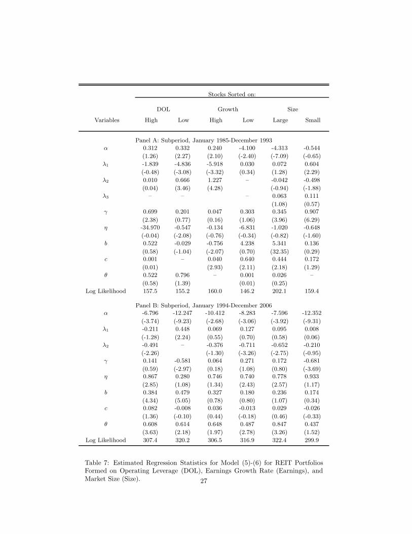
α 0.312 0.332 0.240 -4.100 -4.313 -0.544

(1.26) (2.27) (2.10) (-2.40) (-7.09) (-0.65)

λ1 -1.839 -4.836 -5.918 0.030 0.072 0.604

(-0.48) (-3.08) (-3.32) (0.34) (1.28) (2.29)

λ2 0.010 0.666 1.227 – -0.042 -0.498

(0.04) (3.46) (4.28) (-0.94) (-1.88)

λ3 – – – 0.063 0.111

(1.08) (0.57)γ 0.699 0.201 0.047 0.303 0.345 0.907

(2.38) (0.77) (0.16) (1.06) (3.96) (6.29)

η -34.970 -0.547 -0.134 -6.831 -1.020 -0.648

(-0.04) (-2.08) (-0.76) (-0.34) (-0.82) (-1.60)

b 0.522 -0.029 -0.756 4.238 5.341 0.136

(0.58) (-1.04) (-2.07) (0.70) (32.35) (0.29)c 0.001 – 0.040 0.640 0.444 0.172

(0.01) (2.93) (2.11) (2.18) (1.29)

θ 0.522 0.796 – 0.001 0.026 –

(0.58) (1.39) (0.01) (0.25)

Log Likelihood 157.5 155.2 160.0 146.2 202.1 159.4

Panel B: Subperiod, January 1994-December 2006α -6.796 -12.247 -10.412 -8.283 -7.596 -12.352

(-3.74) (-9.23) (-2.68) (-3.06) (-3.92) (-9.31)

λ1 -0.211 0.448 0.069 0.127 0.095 0.008

(-1.28) (2.24) (0.55) (0.70) (0.58) (0.06)

λ2 -0.491 – -0.376 -0.711 -0.652 -0.210

(-2.26) (-1.30) (-3.26) (-2.75) (-0.95)

γ 0.141 -0.581 0.064 0.271 0.172 -0.681

(0.59) (-2.97) (0.18) (1.08) (0.80) (-3.69)η 0.867 0.280 0.746 0.740 0.778 0.933

(2.85) (1.08) (1.34) (2.43) (2.57) (1.17)

b 0.384 0.479 0.327 0.180 0.236 0.174

(4.34) (5.05) (0.78) (0.80) (1.07) (0.34)

c 0.082 -0.008 0.036 -0.013 0.029 -0.026

(1.36) (-0.10) (0.44) (-0.18) (0.46) (-0.33)

θ 0.608 0.614 0.648 0.487 0.847 0.437

(3.63) (2.18) (1.97) (2.78) (3.26) (1.52)

Log Likelihood 307.4 320.2 306.5 316.9 322.4 299.9

Table 7: Estimated Regression Statistics for Model (5)-(6) for REIT PortfoliosFormed on Operating Leverage (DOL), Earnings Growth Rate (Earnings), andMarket Size (Size). 27

Stocks Sorted on:

DOL Growth Size


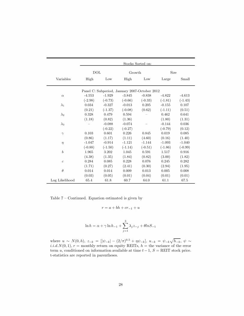
Panel C: Subperiod, January 2007-October 2012α -4.553 -1.929 -3.845 -0.838 -4.822 -4.613

(-2.98) (-0.73) (-0.66) (-0.33) (-1.81) (-1.43)

λ1 0.034 -0.327 -0.013 0.205 -0.155 0.107

(0.21) (-1.37) (-0.08) (0.62) (-1.11) (0.51)

λ2 0.328 0.479 0.594 – 0.462 0.641

(1.18) (0.82) (1.36) (1.80) (1.31)

λ3 – -0.088 -0.074 – -0.144 0.036

(-0.22) (-0.27) (-0.79) (0.12)

γ 0.103 0.601 0.226 0.845 0.019 0.085

(0.86) (1.17) (1.11) (4.60) (0.16) (1.40)

η -1.047 -0.914 -1.121 -1.144 -1.093 -1.040

(-0.88) (-1.50) (-1.14) (-0.51) (-1.86) (-0.99)

b 1.965 3.202 1.045 0.591 1.517 0.916

(4.38) (1.35) (1.84) (0.82) (3.00) (1.82)

c 0.284 0.085 0.228 0.076 0.245 0.282

(1.71) (0.27) (2.41) (0.30) (2.94) (1.95)

θ 0.014 0.014 0.009 0.013 0.005 0.008

(0.03) (0.05) (0.01) (0.04) (0.01) (0.01)

Log Likelihood 65.4 61.8 60.7 64.0 61.1 67.5

Table 7 – Continued. Equation estimated is given by

r = a+ bh+ cr−1 + u

lnh = α+ γ lnh−1 +

3∑

j=1

λjz−j + θlnS−1

where u ∼ N(0, h), z−k = [|ψ−k| − (2/π)0.5 + ηψ−k], u−k = ψ−k

√

h−k, ψ ∼i.i.d.N(0, 1), r = monthly return on equity REITs, h = the variance of the errorterm u, conditioned on information available at time t− 1, S = REIT stock price.t-statistics are reported in parentheses.

28

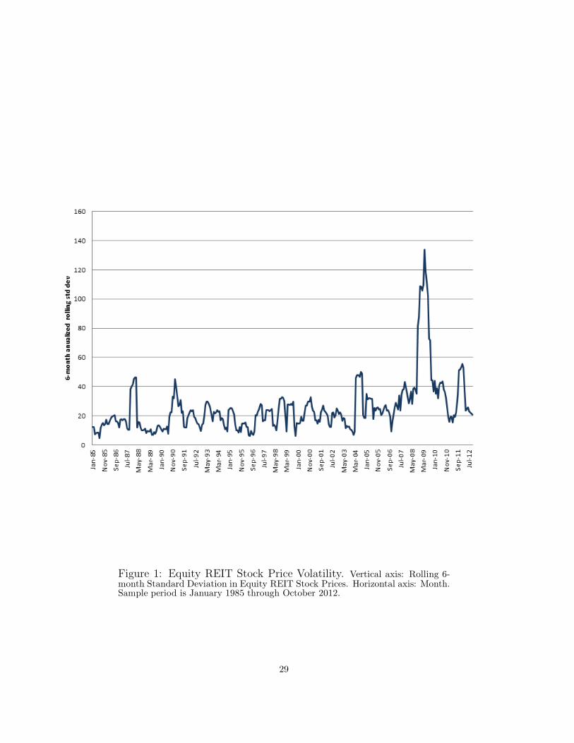
Figure 1: Equity REIT Stock Price Volatility. Vertical axis: Rolling 6-month Standard Deviation in Equity REIT Stock Prices. Horizontal axis: Month.Sample period is January 1985 through October 2012.

29

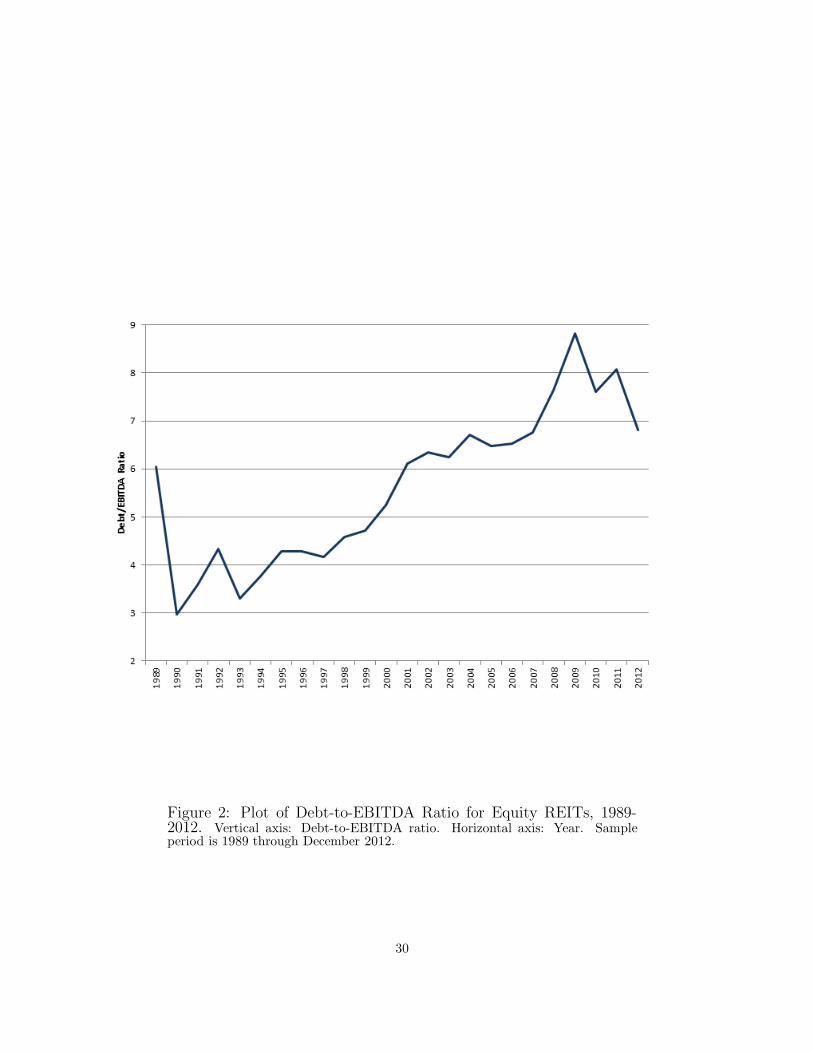
Figure 2: Plot of Debt-to-EBITDA Ratio for Equity REITs, 1989-2012. Vertical axis: Debt-to-EBITDA ratio. Horizontal axis: Year. Sampleperiod is 1989 through December 2012.

30

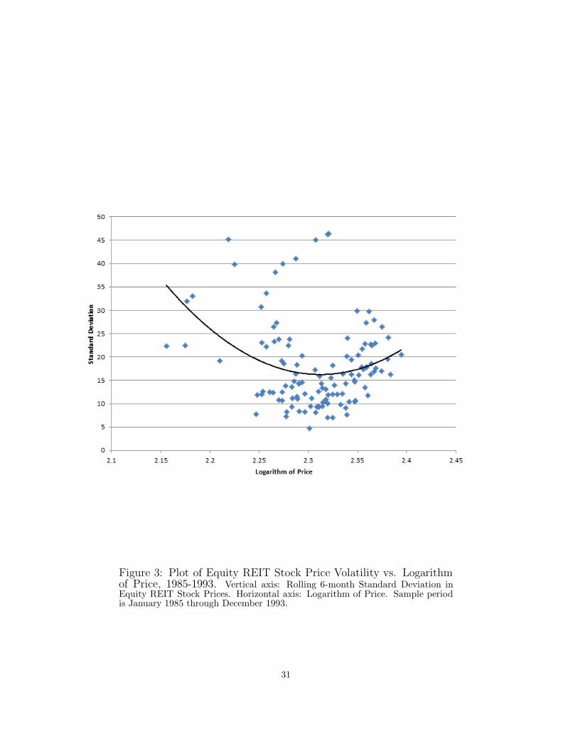
Figure 3: Plot of Equity REIT Stock Price Volatility vs. Logarithmof Price, 1985-1993. Vertical axis: Rolling 6-month Standard Deviation inEquity REIT Stock Prices. Horizontal axis: Logarithm of Price. Sample periodis January 1985 through December 1993.

31

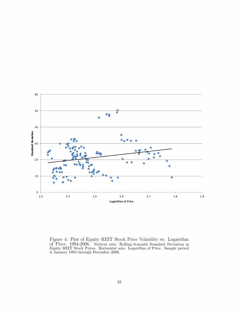
Figure 4: Plot of Equity REIT Stock Price Volatility vs. Logarithmof Price, 1994-2006. Vertical axis: Rolling 6-month Standard Deviation inEquity REIT Stock Prices. Horizontal axis: Logarithm of Price. Sample periodis January 1994 through December 2006.

32

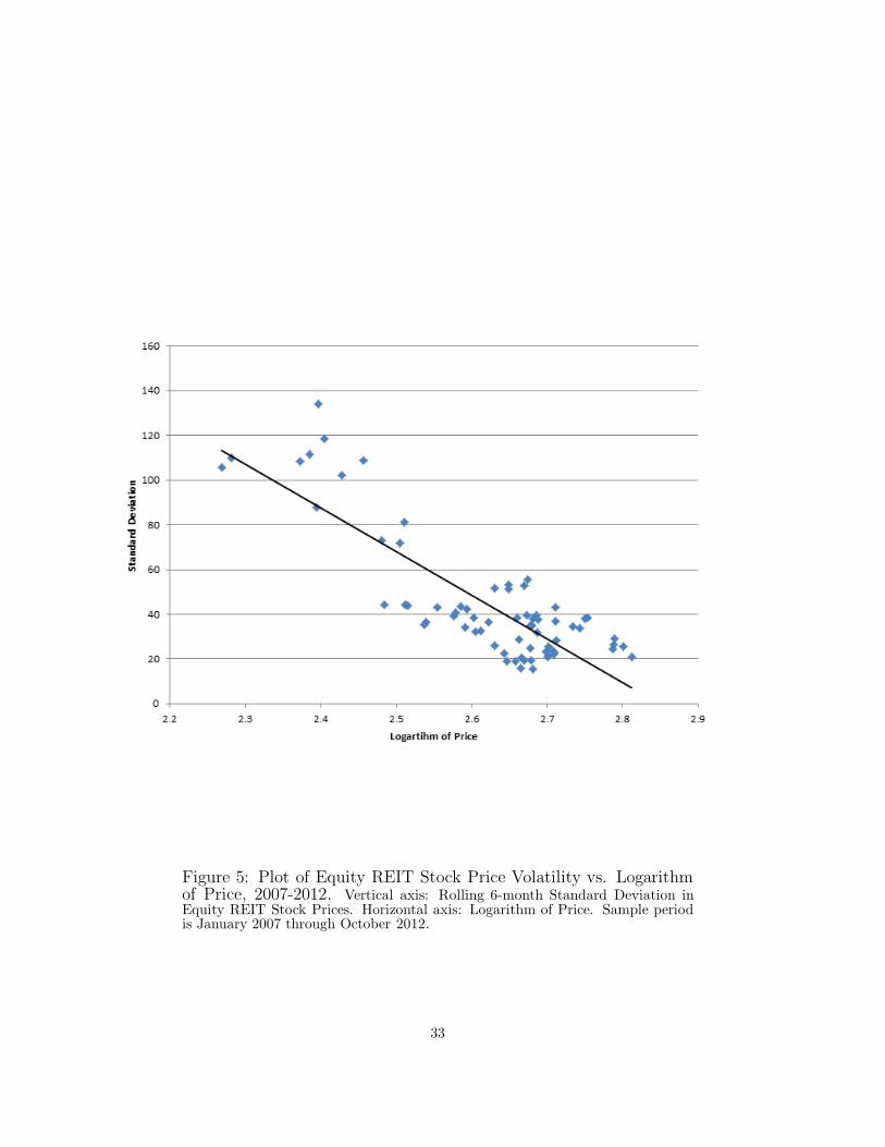
Figure 5: Plot of Equity REIT Stock Price Volatility vs. Logarithmof Price, 2007-2012. Vertical axis: Rolling 6-month Standard Deviation inEquity REIT Stock Prices. Horizontal axis: Logarithm of Price. Sample periodis January 2007 through October 2012.

33

reit stock price volatility during the financial crisis · reit stock price volatility during the...

Documents