Reinforcement Learning to AdjustRobot Movements to New Situations

Jens KoberMPI for Biol. Cybernetics, GermanyEmail: jens.kober@tuebingen.mpg.de

Erhan OztopATR Comput. Neuroscience Labs, Japan

Email: erhan@atr.jp

Jan PetersMPI for Biol. Cybernetics, GermanyEmail: jan.peters@tuebingen.mpg.de

Abstract—Many complex robot motor skills can be representedusing elementary movements, and there exist efficient techniquesfor learning parametrized motor plans using demonstrations andself-improvement. However, in many cases, the robot currentlyneeds to learn a new elementary movement even if a parametrizedmotor plan exists that covers a similar, related situation. Clearly,a method is needed that modulates the elementary movementthrough the meta-parameters of its representation. In this paper,we show how to learn such mappings from circumstances tometa-parameters using reinforcement learning. We introduce anappropriate reinforcement learning algorithm based on a ker-nelized version of the reward-weighted regression. We comparethis algorithm to several previous methods on a toy example andshow that it performs well in comparison to standard algorithms.Subsequently, we show two robot applications of the presentedsetup; i.e., the generalization of throwing movements in darts, andof hitting movements in table tennis. We show that both taskscan be learned successfully using simulated and real robots.

I. INTRODUCTION

In robot learning, motor primitives based on dynamicalsystems [1], [2] allow acquiring new behaviors quickly and re-liably both by imitation and reinforcement learning. Resultingsuccesses have shown that it is possible to rapidly learn motorprimitives for complex behaviors such as tennis-like swings[1], T-ball batting [3], drumming [4], biped locomotion [5],ball-in-a-cup [6], and even in tasks with potential industrialapplications [7]. The dynamical system motor primitives [1]can be adapted both spatially and temporally without changingthe overall shape of the motion. While the examples areimpressive, they do not address how a motor primitive can begeneralized to a different behavior by trial and error withoutre-learning the task. For example, if the string length has beenchanged in a ball-in-a-cup [6] movement1, the behavior has tobe re-learned by modifying the movements parameters. Giventhat the behavior will not drastically change due to a stringlength variation of a few centimeters, it would be better togeneralize that learned behavior to the modified task. Suchgeneralization of behaviors can be achieved by adapting themeta-parameters of the movement representation2.

In machine learning, there have been many attempts touse meta-parameters in order to generalize between tasks [8].

1In this movement, the system has to jerk a ball into a cup where the ballis connected to the bottom of the cup with a string.

2Note that the tennis-like swings [1] could only hit a static ball at the endof their trajectory, and T-ball batting [3] was accomplished by changing thepolicy’s parameters.

Figure 1: This figure illustrates a 2D dart throwing task. Thesituation, described by the state s corresponds to the relativeheight. The meta-parameters γ are the velocity and the angleat which the dart leaves the launcher. The policy parametersrepresent the backward motion and the movement on the arc.The meta-parameter function γ(s), which maps the state tothe meta-parameters, is learned.

Particularly, in grid-world domains, significant speed-up couldbe achieved by adjusting policies by modifying their meta-parameters (e.g., re-using options with different subgoals) [9].In robotics, such meta-parameter learning could be particularlyhelpful due to the complexity of reinforcement learning forcomplex motor skills with high dimensional states and actions.The cost of experience is high as sample generation is timeconsuming and often requires human interaction (e.g., incart-pole, for placing the pole back on the robots hand) orsupervision (e.g., for safety during the execution of the trial).Generalizing a teacher’s demonstration or a previously learnedpolicy to new situations may reduce both the complexity ofthe task and the number of required samples. For example, theoverall shape of table tennis forehands are very similar whenthe swing is adapted to varied trajectories of the incomingball and a different targets on the opponent’s court. Here, thehuman player has learned by trial and error how he has to adaptthe global parameters of a generic strike to various situations[10]. Hence, a reinforcement learning method for acquiringand refining meta-parameters of pre-structured primitive move-ments becomes an essential next step, which we will addressin this paper.

We present current work on automatic meta-parameteracquisition for motor primitives by reinforcement learning.We focus on learning the mapping from situations to meta-

parameters and how to employ these in dynamical systemsmotor primitives. We extend the motor primitives of [1] witha learned meta-parameter function and re-frame the problemas an episodic reinforcement learning scenario. In order toobtain an algorithm for fast reinforcement learning of meta-parameters, we view reinforcement learning as a reward-weighted self-imitation [11], [6].

As it may be hard to realize a parametrized representationfor meta-parameter determination, we reformulate the reward-weighted regression [11] in order to obtain a Cost-regularizedKernel Regression (CrKR) that is related to Gaussian processregression [12]. We compare the Cost-regularized Kernel Re-gression with a traditional policy gradient algorithm [3] andthe reward-weighted regression [11] on a toy problem in orderto show that it outperforms available previously developedapproaches. As complex motor control scenarios, we evaluatethe algorithm in the acquisition of flexible motor primitivesfor dart games such as Around the Clock [13] and for tabletennis.

II. META-PARAMETER LEARNING FOR MOTORPRIMITIVES

The goal of this paper is to show that elementary movementscan be generalized by modifying only the meta-parameters ofthe primitives using learned mappings. In Section II-A, we firstreview how a single primitive movement can be representedand learned. We discuss how such meta-parameters may beable to adapt the motor primitive spatially and temporallyto the new situation. In order to develop algorithms thatlearn to automatically adjust such motor primitives, we modelmeta-parameter self-improvement as an episodic reinforce-ment learning problem in Section II-B. While this problemcould in theory be treated with arbitrary reinforcement learningmethods, the availability of few samples suggests that moreefficient, task appropriate reinforcement learning approachesare needed. To avoid the limitations of parametric functionapproximation, we aim for a kernel-based approach. Whena movement is generalized, new parameter settings need tobe explored. Hence, a predictive distribution over the meta-parameters is required to serve as an exploratory policy.These requirements lead to the method which we derivein Section II-C and employ for meta-parameter learning inSection II-D.

A. Motor Primitives with Meta-Parameters

In this section, we review how the dynamical systems motorprimitives [1], [2] can be used for meta-parameter learning.The dynamical system motor primitives [1] are a powerfulmovement representation that allows ensuring the stability ofthe movement, choosing between a rhythmic and a discretemovement and is invariant under rescaling of both durationand movement amplitude. These modification parameters canbecome part of the meta-parameters of the movement.

In this paper, we focus on single stroke movements whichappear frequently in human motor control [14], [2]. Therefore,we will always focus on the discrete version of the dynamical

system motor primitives in this paper (however, the resultsmay generalize well to rhythmic motor primitives and hybridsettings). We use the most recent formulation of the discretedynamical systems motor primitives [2] where the phase z ofthe movement is represented by a single first order system

z = −ταzz. (1)

This canonical system has the time constant τ = 1/T whereT is the duration of the motor primitive and a parameterαz , which is chosen such that z ≈ 0 at T . Subsequently,the internal state x of a second system is chosen such thatpositions q of all degrees of freedom are given by q = x1,the velocities by q = τx2 = x1 and the accelerations byq = τ x2. The learned dynamics of Ijspeert motor primitivescan be expressed in the following form

x2 = ταx (βx (g − x1)− x2) + τAf (z) , (2)x1 = τx2.

This set of differential equations has the same time constantτ as the canonical system and parameters αx, βx are setsuch that the system is critically damped. The goal param-eter g, a transformation function f and an amplitude ma-trix A = diag (a1, a2, . . . , aI), with the amplitude modifiera = [a1, a2, . . . , aI ] allow representing complex movements.In [2], the authors use a = g−x0

1, with the initial position x01,

which ensures linear scaling. Other choices are possibly bettersuited for specific tasks, see for example [15]. The transfor-mation function f (z) alters the output of the first system, inEquation (1), so that the second system in Equation (2), canrepresent complex nonlinear patterns and is given by

f (z) =∑N

n=1ψn (z) θnz. (3)

Here, θn contains the nth adjustable parameter of all degreesof freedom, N is the number of parameters per degree of free-dom, and ψn(z) are the corresponding weighting functions [2].Normalized Gaussian kernels are used as weighting functionsgiven by

ψn =exp

(−hn (z − cn)2

)∑N

m=1 exp(−hm (z − cm)2

) . (4)

These weighting functions localize the interaction in phasespace using the centers cn and widths hn. As z ≈ 0 at T , theinfluence of the transformation function f (z) in Equation (3)vanishes and the system stays at the goal position g. Notethat the degrees of freedom (DoF) are usually all modeledindependently in the second system in Equation (2). All DoFsare synchronous as the dynamical systems for all DoFs startat the same time, have the same duration and the shape ofthe movement is generated using the transformation f (z) inEquation (3), which is learned as a function of the sharedcanonical system in Equation (1).

One of the biggest advantages of this motor primitive frame-work [1], [2] is that the second system in Equation (2), is linearin the shape parameters θ. Therefore, these parameters canbe obtained efficiently, and the resulting framework is well-suited for imitation [1] and reinforcement learning [6]. The

resulting policy is invariant under transformations of the initialposition x0

1, the goal g, the amplitude A and the duration T[1]. These four modification parameters can be used as themeta-parameters γ of the movement. Obviously, we can makemore use of the motor primitive framework by adjusting themeta-parameters γ depending on the current situation or states according to a meta-parameter function γ(s). The state scan for example contain the current position, velocity andacceleration of the robot and external objects, as well as thetarget to be achieved. This paper focuses on learning the meta-parameter function γ(s) by episodic reinforcement learning.

Illustration of the Learning Problem: As an illustrationof the meta-parameter learning problem, we take a 2D dartthrowing task with a dart on a launcher which is illustrated inFigure 1 (in Section III-B, we will expand this example to arobot application). Here, the desired skill is to hit a specifiedpoint on a wall with a dart. The dart is placed on the launcherand held there by friction. The motor primitive correspondsto the throwing of the dart. When modeling a single dart’smovement with dynamical-systems motor primitives [1], thecombination of retracting and throwing motions would berepresented by one movement primitive and can be learned bydetermining the movement parameters θ. These parameterscan either be estimated by imitation learning or acquiredby reinforcement learning. The dart’s impact position can beadapted to a desired target by changing the velocity and theangle at which the dart leaves the launcher. These variablescan be influenced by changing the meta-parameters of themotor primitive such as the final position of the launcher andthe duration of the throw. The state consists of the currentposition of the hand and the desired position on the target.If the thrower is always at the same distance from the wallthe two positions can be equivalently expressed as the verticaldistance. The meta-parameter function γ(s) maps the state (therelative height) to the meta-parameters γ (the final position gand the duration of the motor primitive T ).

The approach presented in this paper is applicable to anymovement representation that has meta-parameters, i.e., asmall set of parameters that allows to modify the movement.In contrast to [16], [17], [18] our approach does not requireexplicit (re)planning of the motion.

In the next sections, we derive and apply an appropriatereinforcement learning algorithm.

B. Problem Statement: Meta-Parameter Self-Improvement

The problem of meta-parameter learning is to find a stochas-tic policy π(γ|x) = p(γ|s) that maximizes the expected return

J(π) =ˆ

Sp(s)ˆ

Gπ(γ|s)R(s,γ)dγ ds, (5)

where R(s,γ) denotes all the rewards following the selectionof the meta-parameter γ according to a situation described bystate s. The return of an episode is R(s,γ) = T−1

∑Tt=0 r

t

with number of steps T and rewards rt. For a parametrizedpolicy π with parameters w it is natural to first try a policygradient approach such as finite-difference methods, vanilla

Algorithm 1: Meta-Parameter LearningPreparation steps:

Learn one or more motor primitives by imitation and/orreinforcement learning (yields shape parameters θ).

Determine initial state s0, meta-parameters γ0, and cost C0

corresponding to the initial motor primitive.Initialize the corresponding matrices S,Γ,C.Choose a kernel k,K.Set a scaling parameter λ.

For all iterations j:Determine the state sj specifying the situation.Calculate the meta-parameters γj by:

Determine the mean of each meta-parameter iγi(s

j) = k(sj)T (K + λC)−1 Γi,Determine the varianceσ2(sj) = k(sj , sj)− k(sj)T (K + λC)−1 k(sj),

Draw the meta-parameters from a Gaussian distributionγj ∼ N (γ|γ(sj), σ2(sj)I).

Execute the motor primitive using the new meta-parameters.Calculate the cost cj at the end of the episode.Update S,Γ,C according to the achieved result.

policy gradient approaches and natural gradients3. Reinforce-ment learning of the meta-parameter function γ(s) is notstraightforward as only few examples can be generated onthe real system and trials are often quite expensive. The creditassignment problem is non-trivial as the whole movement isaffected by every change in the meta-parameter function. Earlyattempts using policy gradient approaches resulted in tens ofthousands of trials even for simple toy problems, which is notfeasible on a real system.

Dayan & Hinton [19] showed that an immediate rewardcan be maximized by instead minimizing the Kullback-Leiblerdivergence D(π(γ|s)R(s,γ)||π′(γ|s)) between the reward-weighted policy π(γ|s) and the new policy π′(γ|s). Williams[20] suggested to use a particular policy in this context; i.e.,the policy

π(γ|s) = N (γ|γ(s), σ2(s)I),

where we have the deterministic mean policy γ(s) = φ(s)Twwith basis functions φ(s) and parameters w as well as the vari-ance σ2(s) that determines the exploration ε ∼ N (0, σ2(s)I).The parameters w can then be adapted by reward-weightedregression in an immediate reward [11] or episodic rein-forcement learning scenario [6]. The reasoning behind thisreward-weighted regression is that the reward can be treatedas an improper probability distribution over indicator variablesdetermining whether the action is optimal or not.

C. A Task-Appropriate Reinforcement Learning Algorithm

Designing good basis functions is challenging, a nonpara-metric representation is better suited in this context. Thereis an intuitive way of turning the reward-weighted regressioninto a Cost-regularized Kernel Regression. The kernelizationof the reward-weighted regression can be done straightfor-wardly (similar to Section 6.1 of [21] for regular supervisedlearning). Inserting the reward-weighted regression solutionw = (ΦTRΦ + λI)−1ΦTRΓi, and using the Woodburyformula (ΦTRΦ + λI)ΦT = ΦTR(ΦΦT + λR−1), we

3While we will denote the shape parameters by θ, we denote the parametersof the meta-parameter function by w.

−4 −2 0 2 4−4

−3

−2

−1

0

1

2

3(a) Intial Policy based on Prior: R=0

state

met

a−par

amet

er

−4 −2 0 2 4−4

−3

−2

−1

0

1

2

3(b) Policy after 2 updates: R=0.1

state

met

a−par

amet

er

−4 −2 0 2 4−4

−3

−2

−1

0

1

2

3(c) Policy after 9 updates: R=0.8

state

met

a−par

amet

er

−4 −2 0 2 4−4

−3

−2

−1

0

1

2

3(d) Policy after 12 updates: R=0.9

state

met

a−par

amet

er

mean prediction variance training points/cost Gaussian process regression

Figure 2: This figure illustrates the meaning of policy improvements with Cost-regularized Kernel Regression. Each sampleconsists of a state, a meta-parameter and a cost where the cost is indicated the blue error bars. The red line represents theimproved mean policy, the dashed green lines indicate the exploration/variance of the new policy. For comparison, the graylines show standard Gaussian process regression. As the cost of a data point is equivalent to having more noise, pairs of statesand meta-parameter with low cost are more likely to be reproduced than others with high costs.

transform reward-weighted regression into a Cost-regularizedKernel Regression

γi = φ(s)Tw = φ(s)T(ΦTRΦ + λI

)−1

ΦTRΓi

= φ(s)TΦT(ΦΦT + λR−1

)−1

Γi, (6)

where the rows of Φ correspond to the basis functions φ(si) =Φi of the training examples, Γi is a vector containing thetraining examples for meta-parameter component γi, and λ isa ridge factor. Next, we assume that the accumulated rewardsRk are strictly positive Rk > 0 and can be transformed intocosts by ck = 1/Rk. Hence, we have a cost matrix C =R−1 = diag(R−1

1 , . . . , R−1n ) with the cost of all n data points.

After replacing k(s) = φ(s)TΦT and K = ΦΦT, we obtainthe Cost-regularized Kernel Regression

γi = γi(s) = k(s)T (K + λC)−1 Γi,

which gives us a deterministic policy. Here, costs correspondto the uncertainty about the training examples. Thus, a highcost is incurred for being further away from the desiredoptimal solution at a point. In our formulation, a high costtherefore corresponds to a high uncertainty of the predictionat this point.

In order to incorporate exploration, we need to have astochastic policy and, hence, we need a predictive distribution.This distribution can be obtained by performing the policyupdate with a Gaussian process regression and we directly seefrom the kernel ridge regression

σ2(s) = k(s, s) + λ− k(s)T (K + λC)−1 k(s),

where k(s, s) = φ(s)Tφ(s) is the distance of a point to itself.We call this algorithm Cost-regularized Kernel Regression.

The algorithm corresponds to a Gaussian process regressionwhere the costs on the diagonal are input-dependent noisepriors. Gaussian processes have been used previously forreinforcement learning [22] in value function based approacheswhile here we use them to learn the policy.

If several sets of meta-parameters have similarly low coststhe algorithm’s convergence depends on the order of samples.The cost function should be designed to avoid this behaviorand to favor a single set. The exploration has to be restrictedto safe meta-parameters.

D. Meta-Parameter Learning by Reinforcement Learning

As a result of Section II-C, we have a framework of motorprimitives as introduced in Section II-A that we can use forreinforcement learning of meta-parameters as outlined in Sec-tion II-B. We have generalized the reward-weighted regressionpolicy update to instead become a Cost-regularized KernelRegression (CrKR) update where the predictive variance isused for exploration. In Algorithm 1, we show the completealgorithm resulting from these steps.

The algorithm receives three inputs, i.e., (i) a motor prim-itive that has associated meta-parameters γ, (ii) an initial ex-ample containing state s0, meta-parameter γ0 and cost C0, aswell as (iii) a scaling parameter λ. The initial motor primitivecan be obtained by imitation learning [1] and, subsequently,improved by parametrized reinforcement learning algorithmssuch as policy gradients [3] or Policy learning by WeightingExploration with the Returns (PoWER) [6]. The demonstrationalso yields the initial example needed for meta-parameterlearning. While the scaling parameter is an open parameter, itis reasonable to choose it as a fraction of the average cost andthe output noise parameter (note that output noise and otherpossible hyper-parameters of the kernel can also be obtainedby approximating the unweighted meta-parameter function).

Illustration of the Algorithm: In order to illustrate thisalgorithm, we will use the example of the 2D dart throwingtask introduced in Section II-A. Here, the robot should throwdarts accurately while not destroying its mechanics. Hence,the cost corresponds to the error between desired goal andthe impact point, as well as the absolute velocity of the end-effector. The initial policy is based on a prior, illustrated inFigure 2(a), that has a variance for initial exploration (it oftenmakes sense to start with a uniform prior). This variance isused to enforce exploration. To throw a dart, we sample themeta-parameters from the policy based on the current state4.After the trial the cost is determined and, in conjunction with

4In the dart setting, we could choose the next target and thus employ CrKRas an active learning approach by picking states with large variances. However,often the state is determined by the environment, e.g., the ball trajectory inthe table tennis experiment (Section III-C) depends on the opponent.

102

104

106

20

30

40

50

60

70

80

90

100

number of rollouts

aver

age

cost

(a) Velocity

102

104

106

0

0.5

1

1.5

2

number of rollouts

aver

age

cost

(b) Precision

102

104

106

0.5

1

1.5

2

2.5

3

number of rollouts

aver

age

cost

(c) Combined

Finite Difference Gradient Reward−weighted Regression Cost−regularized Kernel Regression

Figure 3: This figure shows the performance of the compared algorithms averaged over 10 complete learning runs. Cost-regularized Kernel Regression finds solutions with the same final performance two orders of magnitude faster than the finitedifference gradient (FD) approach and twice as fast as the reward-weighted regression. At the beginning FD often is highlyunstable due to our attempts of keeping the overall learning speed as high as possible to make it a stronger competitor. Thelines show the median and error bars indicate standard deviation. The initialization and the initial costs are identical for allapproaches. However, the omission of the first twenty rollouts was necessary to cope with the logarithmic rollout axis.

the employed meta-parameters, used to update the policy5. Ifthe cost is large (for example the impact is far from the target),the variance of the policy is large as it may still be improvedand therefore needs exploration. Furthermore, the mean of thepolicy is shifted only slightly towards the observed exampleas we are uncertain about the optimality of this action. Ifthe cost is small, we know that we are close to an optimalpolicy and only have to search in a small region around theobserved trial. The effects of the cost on the mean and thevariance are illustrated in Figure 2(b). Each additional samplerefines the policy and the overall performance improves (seeFigure 2(c)). If a state is visited several times and differentmeta-parameters are sampled, the policy update must favorthe meta-parameters with lower costs. Algorithm 1 exhibitsthis behavior as illustrated in Figure 2(d).

III. EVALUATION

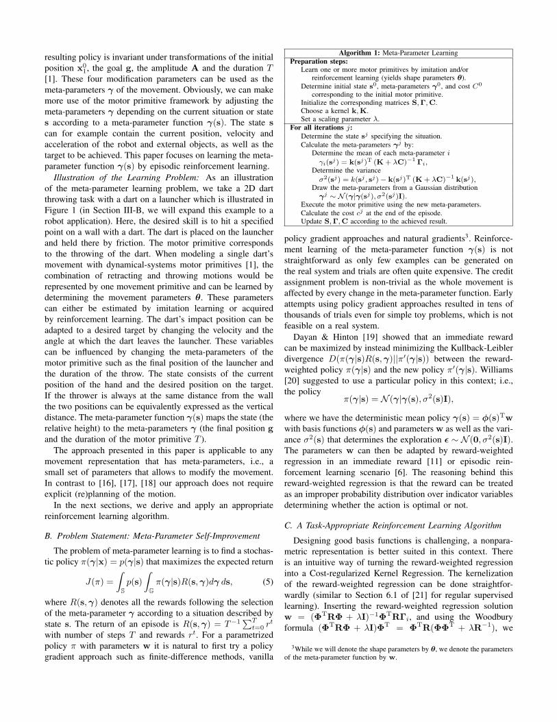
In Section II, we have introduced both a framework formeta-parameter self-improvement as well as an appropriatereinforcement learning algorithm used in this framework. Inthis section, we will first show that the presented reinforcementlearning algorithm yields higher performance than off-the shelfapproaches. Hence, we compare it on a simple planar cannonshooting problem [23] with the preceding reward-weightedregression and an off-the-shelf finite difference policy gradientapproach.

5In the dart throwing example we have a correspondence between the stateand the outcome similar to a regression problem. However, the mappingbetween the state and the meta-parameter is not unique. The same height canbe achieved by different combinations of velocities and angles. Averagingthese combinations is likely to generate inconsistent solutions. The regressionmust hence favor the meta-parameters with the lower costs. CrKR can beemployed as a regularized regression method in this setting.

The proposed reinforcement learning method only requires a cost associatedwith the outcome of the trial. In the table tennis experiment (Section III-C),the state corresponds to the position and velocity of the ball over the net.We only observe the cost related to how well we hit the ball. After a tabletennis trial, we do not know which state would have matched the employedmeta-parameters, as would be required in a regression setting.

The resulting meta-parameter learning framework can beused in a variety of settings in robotics. We consider two sce-narios here, i.e., (i) dart throwing with a simulated robot arm,a real Barrett WAM and the JST-ICORP/SARCOS humanoidrobot CBi, and (ii) table tennis with a simulated robot armand a real Barrett WAM. Some of the real-robot experimentsare still partially work in progress.

A. Benchmark Comparison

In the first task, we only consider a simple simulated planarcannon shooting where we benchmark our ReinforcementLearning by Cost-regularized Kernel Regression approachagainst a finite difference gradient estimator and the reward-weighted regression. Here, we want to learn an optimal policyfor a 2D toy cannon environment similar to [23].

The setup is given as follows: A toy cannon is at a fixedlocation [0.0, 0.1]m. The meta-parameters are the angle withrespect to the ground and the speed of the cannon ball. Inthis benchmark we do not employ the motor primitives butset the parameters directly. The flight of the canon ball issimulated as ballistic flight of a point mass with Stokes’sdrag as wind model. The cannon ball is supposed to hit theground at a desired distance. The desired distance [1..3]mand the wind speed [0..1]m/s, which is always horizontal,are used as input parameters, the velocities in horizontal andvertical directions are predicted (which influences the angleand the speed of the ball leaving the cannon). Lower speedcan be compensated by a larger angle. Thus, there are differentpossible policies for hitting a target; we intend to learn theone which is optimal for a given cost function. This costfunction consists of the sum of the squared distance betweenthe desired and the actual impact point and one hundredth ofthe squared norm of the velocity at impact of the cannon ball.It corresponds to maximizing the precision while minimizingthe employed energy according to the chosen weighting. Allapproaches performed well in this setting, first driving theposition error to zero and, subsequently, optimizing the impact

(a) The dart is placed onthe launcher.

(b) The arm movesback.

(c) The arm moves for-ward on an arc.

(d) The arm stops. (e) The dart is carriedon by its momentum.

(f) The dart hits theboard.

Figure 4: This figure shows a dart throw in a physically realistic simulation.

(a) The dart is placed inthe hand.

(b) The arm movesback.

(c) The arm moves for-ward on an arc.

(d) The arm continuesmoving.

(e) The dart is releasedand the arm followsthrough.

(f) The arm stops andthe dart hits the board.

Figure 5: This figure shows a dart throw on the real JST-ICORP/SARCOS humanoid robot CBi.

velocity. The experiment was initialized with [1, 10]m/s asinitial ball velocities and 1m/s as wind velocity. This settingcorresponds to a very high parabola, which is far from optimal.For plots, we evaluate the policy on a test set of 25 uniformlyrandomly chosen points that remain the same throughout ofthe experiment and are never used in the learning process butonly to generate Figure 3.

We compare our novel algorithm to a finite differencepolicy gradient (FD) method [3] and to the reward-weightedregression (RWR) [11]. The FD method uses a parametricpolicy that employs radial basis functions in order to representthe policy and adds Gaussian exploration. The learning rateas well as the magnitude of the perturbations were tuned forbest performance. We used 51 sets of uniformly perturbedparameters for each update step. The FD algorithm convergesafter approximately 2000 batch gradient evaluations, whichcorresponds to 2, 550, 000 shots with the toy cannon.

The RWR method uses the same parametric policy as thefinite difference gradient method. Exploration is achieved byadding Gaussian noise to the mean policy . All open param-eters were tuned for best performance. The RWR algorithmconverges after approximately 40, 000 shots with the toy can-non. For the Cost-regularized Kernel Regression (CrKR) theinputs are chosen randomly from a uniform distribution. Weuse Gaussian kernels and the open parameters were optimizedby cross-validation on a small test set prior to the experiment.Each trial is added as a new training point if it landed in thedesired distance range. The CrKR algorithm converges afterapproximately 20, 000 shots with the toy cannon.

After convergence, the costs of CrKR are the same as forRWR and slightly lower than those of the FD method. TheCrKR method needs two orders of magnitude fewer shotsthan the FD method. The RWR approach requires twice theshots of CrKR demonstrating that a non-parametric policy, asemployed by CrKR, is better adapted to this class of problemsthan a parametric policy. The squared error between the actualand desired impact is approximately 5 times higher for the

finite difference gradient method, see Figure 3.

B. Dart-Throwing

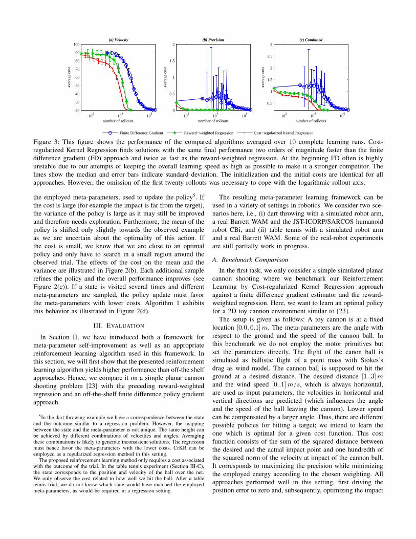
Now, we turn towards the complete framework, i.e., weintend to learn the meta-parameters for motor primitives indiscrete movements. We compare the Cost-regularized KernelRegression (CrKR) algorithm to the reward-weighted regres-sion (RWR). As a sufficiently complex scenario, we chose arobot dart throwing task inspired by [23]. However, we takea more complicated scenario and choose dart games suchas Around the Clock [13] instead of simple throwing at afixed location. Hence, it will have an additional parameterin the state depending on the location on the dartboard thatshould come next in the sequence. The acquisition of a basicmotor primitive is achieved using previous work on imitationlearning [1]. Only the meta-parameter function is learned usingCrKR or RWR.

The dart is placed on a launcher attached to the end-effectorand held there by stiction. We use the Barrett WAM robot armin order to achieve the high accelerations needed to overcomethe stiction. See Figure 4, for a complete throwing movement.The motor primitive is trained by imitation learning withkinesthetic teach-in. We use the Cartesian coordinates withrespect to the center of the dart board as inputs. The parameterfor the final position, the duration of the motor primitive andthe angle around the vertical axis are the meta-parameters.The popular dart game Around the Clock requires the playerto hit the numbers in ascending order, then the bulls-eye.As energy is lost overcoming the stiction of the launchingsled, the darts fly lower and we placed the dartboard lowerthan official rules require. The cost function is the sum often times the squared error on impact and the velocity of themotion. After approximately 1000 throws the algorithms haveconverged but CrKR yields a high performance already muchearlier (see Figure 6). We again used a parametric policy withradial basis functions for RWR. Designing a good parametricpolicy proved very difficult in this setting as is reflected bythe poor performance of RWR.

0 200 400 600 800 1000

0.2

0.4

0.6

0.8

1

1.2

1.4

number of rollouts

aver

age

cost

Cost−regularized Kernel RegressionReward−weighted Regression

Figure 6: This figure shows the cost function of the dart-throwing task for a whole game Around the Clock in eachrollout. The costs are averaged over 10 runs with the error-bars indicating standard deviation.

This experiment is also being carried out on two real,physical robots, i.e., a Barrett WAM and the humanoid robotCBi (JST-ICORP/SARCOS). CBi was developed within theframework of the JST-ICORP Computational Brain Project atATR Computational Neuroscience Labs. The hardware of therobot was developed by the American robotic developmentcompany SARCOS. CBi can open and close the fingers whichhelps for more human-like throwing instead of the launcheremployed by the Barrett WAM. See Figure 5 for a throwingmovement. Parts of these experiments are still in-progress.

C. Table Tennis

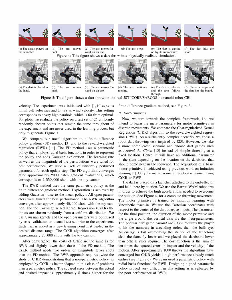
In the second evaluation of the complete framework, we useit for hitting a table tennis ball in the air. The setup consistsof a ball gun that serves to the forehand of the robot, a BarrettWAM and a standard sized table. The movement of the robothas three phases. The robot is in a rest posture and startsto swing back when the ball is launched. During this swing-back phase, the open parameters for the stroke are predicted.The second phase is the hitting phase which ends with thecontact of the ball and racket. In the final phase the robotgradually ends the stroking motion and returns to the restposture. See Figure 8 for an illustration of a complete episode.The movements in the three phases are represented by motorprimitives obtained by imitation learning.

The meta-parameters are the joint positions and velocitiesfor all seven degrees of freedom at the end of the secondphase (the instant of hitting the ball) and a timing parameterthat controls when the swing back phase is transitioning tothe hitting phase. We learn these 15 meta-parameters as afunction of the ball positions and velocities when it is over thenet. We employed a Gaussian kernel and optimized the openparameters according to typical values for the input and output.As cost function we employ the metric distance between thecenter of the paddle and the center of the ball at the hittingtime. The policy is evaluated every 50 episodes with 25 balllaunches picked randomly at the beginning of the learning. Weinitialize the behavior with five successful strokes observedfrom another player. After initializing the meta-parameterfunction with only these five initial examples, the robot missesca. 95% of the balls as shown in Figure 7. Trials are only used

0 200 400 600 800 1000

0.1

0.3

0.5

0.7

0.9

number of rollouts

aver

age

cost

/suc

cess

SuccessCost

Figure 7: This figure shows the cost function of the tabletennis task averaged over 10 runs with the error-bars indicatingstandard deviation. The red line represents the percentage ofsuccessful hits and the blue line the average cost. At thebeginning the robot misses the ball 95% of the episodes andon average by 50 cm. At the end of the learning the robot hitsalmost all balls.

to update the policy if the robot has successfully hit the ball.Figure 9 illustrates different positions of the ball the policy iscapable of dealing with after the learning. Figure 7 illustratesthe costs over all episodes. Preliminary results suggest that theresulting policy performs well both in simulation and for thereal system. We are currently in the process of executing thisexperiment also on the real Barrett WAM.

IV. CONCLUSION & FUTURE WORK

In this paper, we have studied the problem of meta-parameter learning for motor primitives. It is an essentialstep towards applying motor primitives for learning complexmotor skills in robotics more flexibly. We have discussedan appropriate reinforcement learning algorithm for mappingsituations to meta-parameters.

We show that the necessary mapping from situation tometa-parameter can be learned using a Cost-regularized KernelRegression (CrKR) while the parameters of the motor primi-tive can still be acquired through traditional approaches. Thepredictive variance of CrKR is used for exploration in on-policy meta-parameter reinforcement learning. We comparethe resulting algorithm in a toy scenario to a policy gradientalgorithm with a well-tuned policy representation and thereward-weighted regression. We show that our CrKR algorithmcan significantly outperform these preceding methods. Todemonstrate the system in a complex scenario, we have chosenthe Around the Clock dart throwing game and table tennisimplemented both on simulated and real robots.

Adapting movements to situations is also discussed in [16]in a supervised learning setting. Their approach is based onpredicting a trajectory from a previously demonstrated set andrefining it by motion planning. The authors note that kernelridge regression performed poorly for the prediction if the newsituation is far from previously seen ones as the algorithmyields the global mean. In our approach we employ a costweighted mean that overcomes this problem. If the situationis far from previously seen ones, large exploration will helpto find a solution.

(a) The robot is the rest pos-ture.

(b) The arm swings back. (c) The arm strikes the ball. (d) The arm follows throughand decelerates.

(e) The arm returns to therest posture.

Figure 8: This figure shows a table tennis stroke on the real Barrett WAM.

(a) Left. (b) Half left. (c) Center high. (d) Center low. (e) Right.Figure 9: This figure shows samples of the learned forehands. Note that this figure only illustrates the learned meta-parameterfunction in this context but cannot show timing and velocity and it requires a careful observer to note the important configurationdifferences resulting from the meta-parameters.

Future work will require to sequence different motor prim-itives by a supervisory layer. This supervisory layer wouldfor example in a table tennis task decide between a forehandmotor primitive and a backhand motor primitive, the spatialmeta-parameter and the timing of the motor primitive wouldbe adapted according to the incoming ball, and the motorprimitive would generate the trajectory. This supervisory layercould be learned by an hierarchical reinforcement learningapproach [24] (as introduced in the early work by [25]).In this framework, the motor primitives with meta-parameterfunctions could be seen as robotics counterpart of options [9]or macro-actions [26].

REFERENCES

[1] A. J. Ijspeert, J. Nakanishi, and S. Schaal, “Learning attractor landscapesfor learning motor primitives,” in Advances in Neural InformationProcessing Systems 16, 2003.

[2] S. Schaal, P. Mohajerian, and A. J. Ijspeert, “Dynamics systems vs.optimal control — a unifying view,” Progress in Brain Research,vol. 165, no. 1, pp. 425–445, 2007.

[3] J. Peters and S. Schaal, “Policy gradient methods for robotics,” in Proc.Int. Conf. Intelligent Robots and Systems, 2006.

[4] D. Pongas, A. Billard, and S. Schaal, “Rapid synchronization andaccurate phase-locking of rhythmic motor primitives,” in Proc. Int. Conf.Intelligent Robots and Systems, 2005.

[5] J. Nakanishi, J. Morimoto, G. Endo, G. Cheng, S. Schaal, andM. Kawato, “Learning from demonstration and adaptation of bipedlocomotion,” Robotics and Autonomous Systems, vol. 47, no. 2-3,pp. 79–91, 2004.

[6] J. Kober and J. Peters, “Policy search for motor primitives in robotics,”in Advances in Neural Information Processing Systems 22, 2009.

[7] H. Urbanek, A. Albu-Schäffer, and P. van der Smagt, “Learning fromdemonstration repetitive movements for autonomous service robotics,”in Proc. Int. Conf. Intelligent Robots and Systems, 2004.

[8] R. Caruana, “Multitask learning,” Machine Learning, vol. 28, pp. 41–75,1997.

[9] A. McGovern and A. G. Barto, “Automatic discovery of subgoalsin reinforcement learning using diverse density,” in Proc. Int. Conf.Machine Learning, 2001.

[10] K. Mülling, “Motor control and learning in table tennis,” Master’s thesis,University of Tübingen, 2009.

[11] J. Peters and S. Schaal, “Reinforcement learning by reward-weightedregression for operational space control,” in Proc. Int. Conf. MachineLearning, 2007.

[12] C. E. Rasmussen and C. K. Williams, Gaussian Processes for MachineLearning. MIT Press, 2006.

[13] Masters Games Ltd., “The rules of darts,” onlinehttp://www.mastersgames.com/rules/darts-rules.htm, July 2010.

[14] G. Wulf, Attention and motor skill learning. Champaign, IL: HumanKinetics, 2007.

[15] D.-H. Park, H. Hoffmann, P. Pastor, and S. Schaal, “Movement repro-duction and obstacle avoidance with dynamic movement primitives andpotential fields,” in Proc. Int. Conf. Humanoid Robots, 2008.

[16] N. Jetchev and M. Toussaint, “Trajectory prediction: learning to mapsituations to robot trajectories,” in Proc. Int. Conf. Machine Learning,2009.

[17] D. B. Grimes and R. P. N. Rao, “Learning nonparametric policies byimitation,” in Proc. Int. Conf. Intelligent Robots and System, 2008.

[18] D. C. Bentivegna, A. Ude, C. G. Atkeson, and G. Cheng, “Learning toact from observation and practice,” Int. Journal of Humanoid Robotics,vol. 1, no. 4, pp. 585–611, 2004.

[19] P. Dayan and G. E. Hinton, “Using expectation-maximization for rein-forcement learning,” Neural Computation, vol. 9, no. 2, pp. 271–278,1997.

[20] R. J. Williams, “Simple statistical gradient-following algorithms for con-nectionist reinforcement learning,” Machine Learning, vol. 8, pp. 229–256, 1992.

[21] C. M. Bishop, Pattern Recognition and Machine Learning. SpringerVerlag, 2006.

[22] Y. Engel, S. Mannor, and R. Meir, “Reinforcement learning withgaussian processes,” in Proc. Int. Conf. Machine Learning, 2005.

[23] G. Lawrence, N. Cowan, and S. Russell, “Efficient gradient estimationfor motor control learning,” in Proc. Int. Conf. Uncertainty in ArtificialIntelligence, 2003.

[24] A. Barto and S. Mahadevan, “Recent advances in hierarchical reinforce-ment learning,” Discrete Event Dynamic Systems, vol. 13, no. 4, pp. 341– 379, 2003.

[25] M. Huber and R. Grupen, “Learning robot control using control policiesas abstract actions,” in NIPS’98 Workshop: Abstraction and Hierarchyin Reinforcement Learning, 1998.

[26] A. McGovern, R. S. Sutton, and A. H. Fagg, “Roles of macro-actionsin accelerating reinforcement learning,” in Grace Hopper Celebrationof Women in Computing, 1997.