reinforcement learning for autonomous driving obstacle ... · reinforcement learning for autonomous...

Reinforcement Learning for Autonomous Driving Obstacle Avoidance usingLIDAR

Lucas Manuelli [email protected]

Massachusetts Institute of Technology

Pete Florence [email protected]

Massachusetts Institute of Technology

1. IntroductionIn this project we evaluate the ability of several reinforce-ment learning methods to autonomously drive a car througha cluttered environment. We don’t assume a map of theenvironment a priori but rather rely on our sensor (in thiscase a LIDAR) to inform control decisions. A standard ap-proach to solving this problem would require building up amap of the environment, possibly using an occupancy grid,and then planning a collision free path through this esti-mated map using a planner such as RRT*. On the otherhand one notes that simple output feedback controllers,such as Braitenberg controllers, can be quite effective forobstacle avoidance tasks. Guided by this example we wantto see how reinforcement learning performs in learning anoutput feedback controller for obstacle avoidance.

Our initial goal was to implement a value-based learningmethod, and we were recommended to start with SARSA.After some initial encouraging results with SARSA, wedecided implemented Q-learning and a continuous state-space version SARSA using function approximation. Inaddition we also tried policy search methods.

In short, there were distinct advantages and concerns foundfor the different approaches. The value-function-basedapproaches benefit greatly from their dynamic program-ming formulation, but it is also their limitation, particularlydue to the difficulties of discretization. The policy-search-based approaches have some nice properties including thatthey are easy to “seed” with a favorable initialization, anddo not need to be discretized, but do not benefit from Bell-man’s optimality principle (even if it does not hold, giventhe non-Markov observable state). In most cases, the abilityof the reinforcement learning agents to improve their per-formance, even if not without “hand-holding” from us, isquite remarkable to watch. That said, significant effort andtuning is required, and in the end, we were not able to satis-fiably outperform intuitive hand-designed controllers. Thedynamic programming techniques had a ceiling of perfor-mance imposed by the discretization, and the policy search

methods were not able to improve upon essentially-perfecthand-designed controllers. Although this was the case forthe study presented, it seems that in scenarios where intu-ition is less readily applied, and/or with more patient tuningof parameters, even better results may be obtained for thereinforcement learning controllers.

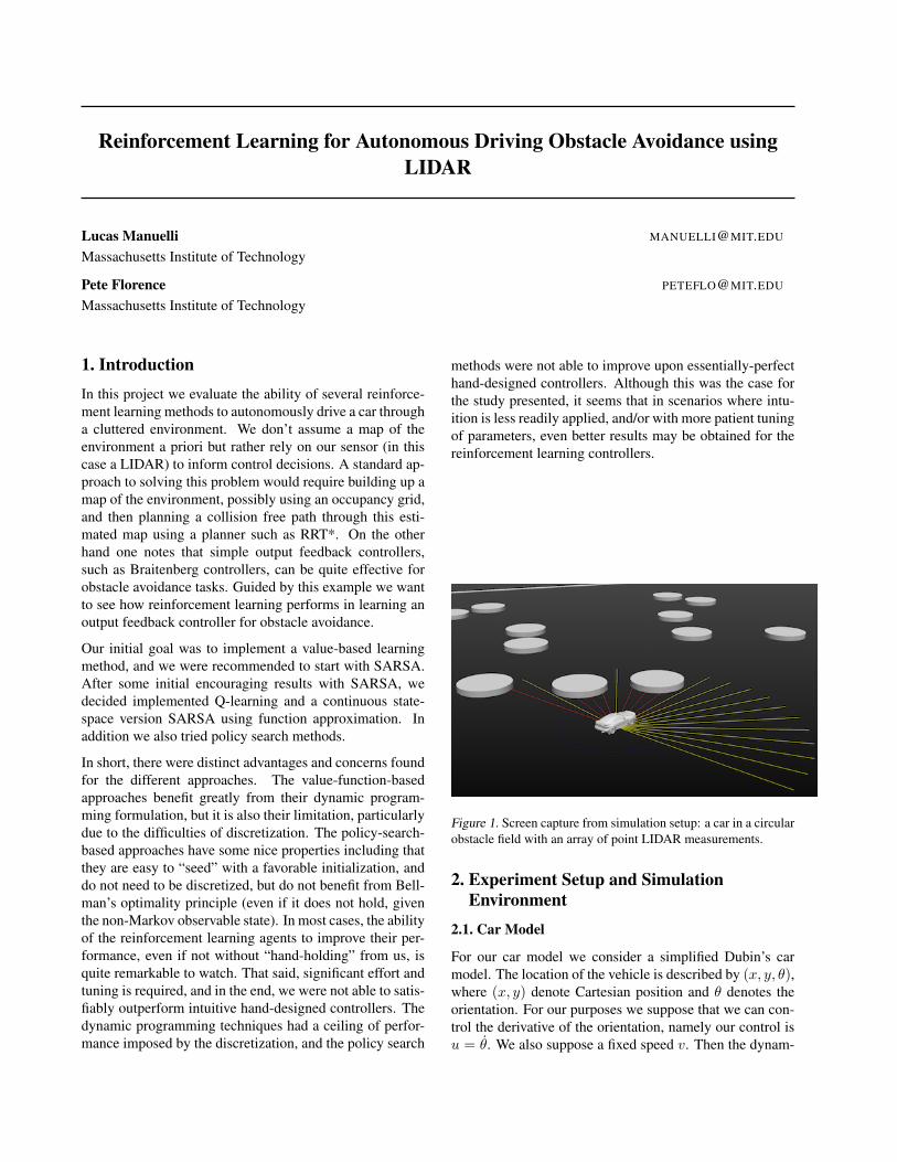
Figure 1. Screen capture from simulation setup: a car in a circularobstacle field with an array of point LIDAR measurements.

2. Experiment Setup and SimulationEnvironment

2.1. Car Model

For our car model we consider a simplified Dubin’s carmodel. The location of the vehicle is described by (x, y, ✓),where (x, y) denote Cartesian position and ✓ denotes theorientation. For our purposes we suppose that we can con-trol the derivative of the orientation, namely our control isu =

˙

✓. We also suppose a fixed speed v. Then the dynam-

RL for Obstacle Avoidance

ics of the vehicle are given by

x = v cos(✓) (1)y = v sin(✓) (2)˙

✓ = u (3)

2.2. Sensor Model

For our sensor model we use a small array of point LI-DARs. In particular, N beams are spread evenly over thefield of view [✓

min

, ✓

max

]. All experiments shown useN = 20 and [✓

min

= �⇡, ✓max

= ⇡]. Each laser has amaximum range of d

max

. The n

th laser then returns x

n

,which is the distance to the first obstacle it encounters, ord

max

if no obstacle is detected. Then one laser measure-ment can be summarized as X = (x1, . . . , xN

).

2.3. Obstacle Environment

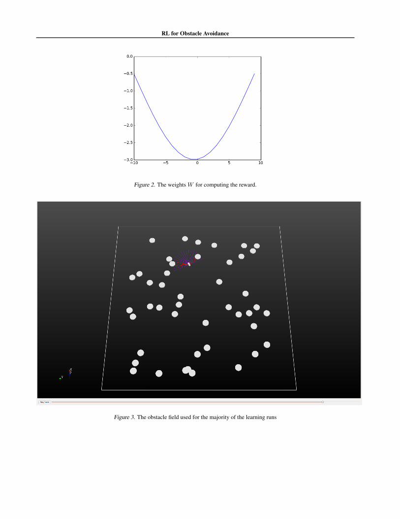
Picking the right obstacle environment for our task requiredsome trial-and-error. Obstacles that were too thin alongone direction were not a good choice, as they could hidein between the “array of point LIDARs” as the robot ap-proached. Thus circular obstacles were chosen, as theycircumvented this problem. Picking the right density ofobstacles and obstacle size was another trial-and-error pro-cess. A square border prevented the car from escaping. Alisting of approximate parameters for the obstacle environ-ments used is provided in Table 1. Generalizations acrossobstacle environments is outside the scope of this project.

Car parametersCar velocity, v 16 m/sMaximum turning rate, u

max

4 rad/s

Sensor parametersNumber of point LIDARS, N 20Maximum laser range, d

max

10 mField of view [✓

min

, ✓

max

] [�⇡,⇡]

Obstacle environment parametersArea of square world 250 m

2

Obstacle density 0.18 / m2 (45 obstacles in 250 m

2)Circular obstacle radius 1.75 m

Table 1. Simulation parameters used for the experiments, unlessotherwise noted.

2.4. Simulation Environment

Our software stack is integrated with a robotics visualiza-tion tool called Director (Marion, 2015). We use the Direc-tor code for visualization and raycasting. This is the onlyexternal code that we use in addition to standard Pythonmodules. Our simulation environment is written in Python.We have a main class called Simulator which com-bines together several other modules, e.g. Car, Sensor,World, Controller, Reward, Sarsa, etc, to con-struct a working simulation class. All of this code was

written by us for the project. As mentioned before, theonly fundamental pieces of code that we didn’t write werethe visualization tools and the raycasting method whichwe use for computing our sensor model. One nice fea-ture of the Director application is that it uses VisualizationToolkit as the underlying graphics engine, and thus our ray-cast calls are actually in C++ and thus very efficient. Weuse a timestep of dt = 0.05 in all our experiments, andscipy.integrate is used to for integrating forward thedynamics.

All of the code for this project is open-source andmay be found at github.com/peteflorence/

Machine-Learning-6.867-homework. We alsostrongly encourage readers to watch our YouTube video,linked from the GitHub repo, which displays the controllersin action, from the learning phase through to final learnedcontrollers.

2.5. Braitenberg (Hand-Designed) Controller

As a baseline against which to compare our learned con-trollers, we used a simple hand-designed controller inspiredby the controllers of Valentino Braitenberg. The most basiccontroller we tried simply counts the number of non-maxsensor returns on the left (n

left

=

PN/2i

[x

i

< d

max

])and compares with the number of non-max sensor re-turns on the right (n

right

=

PN

i=N/2+1 [x

i

< d

max

]),and then selects the action to turn towards the directionmin(n

left

, n

right

). If no obstacles are seen (nleft

=

n

right

= 0), then the controller selects to go straight.Thus the action space for this simple controller is A =

{umax

, 0,�umax

}. This controller actually works surpris-ingly well.

The best Braitenberg-style controller we used is a slightimprovement on the above version: it actually takes intothe account the distances measured. This controller usesthe squared inverse of each of the sensor measurements asits features: �

B

(x

i

) =

1x

2i

. The sum of these features isthen computed for the left and right, and again the action isselected to turn towards the direction min(n

left

, n

right

).An algorithm description is provided (Algorithm 1).

github.com/peteflorence/Machine-Learning-6.867-homework

github.com/peteflorence/Machine-Learning-6.867-homework


Algorithm 1 Braitenberg Squared Inverse Controller(BSIC)

Input: sensor data x

i

, size N

Output: u from A = {umax

, 0,�umax

}Initialize n

left

, nright

= 0

for i = 1 to N/2 don

left

= n

left

+ 1/(x

i

)

2

end forfor i = N/2 + 1 to N don

right

= n

right

+ 1/(x

i

)

2

end forif n

left

> n

right

thenu = u

max

(TURN LEFT)else

if nleft

< n

right

thenu = �u

max

(TURN RIGHT)elseu = 0 (GO STRAIGHT)

end ifend if

3. Dynamic Programming: SARSA andQ-Learning

Two of the most popular methods in reinforcement learn-ing are SARSA and Q-Learning. These methods both aimto find the optimal policy of a dynamic programming prob-lem. Thus the first step is to reformulate our problem as adynamic programming problem.

3.1. Dynamic Programming Formulation

To formulate our problem as a dynamic programming prob-lem we need to define a “state.” Let S

c

= (x, y, ✓) be thestate of the car, and let X = (x1, . . . , xn

) be the sensorstate. What we can observe is S

c

and X . On the otherhand the “true state” includes a complete description of theglobal map. If we don’t give our learning algorithm a priormap and only let it have measurements of S

c

and X , thenit is clear that the “true state” is partially observable. Tomake our problem similar to the limitations of a real carrobot with just the described LIDAR sensor model, we onlyallow our reinforcement learning agent to access X , and sowe consider S = X (this is because the dynamics of the carare trivial here). Since this is not a state in the true senseof the word let us call it a “reward state” (really it’s just theobservation). Next we need to define our action set. In prin-ciple our model has a continuous action set. However, forthe purposes of SARSA and Q-Learning it is much easierto have a discrete action space. Thus we restrict ourselvesto a 2 {u

max

, 0,�umax

} = A, which correspond to left,straight, and right actions. Let ✓

n

be the angle of nth laserwhere ✓

n

= 0 corresponds to straight ahead. Now we need

to define the reward function. First define weights

w

n

= C0 + cos(✓

n

) (4)

Also define

�(x

n

) =

(min(1/x

n

, C

max

) x

n

< d

max

0 x

n

= d

max

(5)

Then � has the effect of amplifying short distance mea-surements. Let W =

C

raycastPn

w

n

· (w1, . . . , wN

), �(X) =

(�(x1), . . . ,�(xn

)). Then define the reward R(S, a) as

R(S, a) = C

action

|a|+ hW,�(X)i (6)

where C

action

is an action cost. Finally if the car is cur-rently in collision with an obstacle, i.e. some laser x

n

isreading less than d

min

then we set R(S, a) = C

collision

.

Now let us think about why this may be a reasonable re-ward function for our objective, which is obstacle avoid-ance. One should think of C

raycast

, C

action

, C

collision

< 0

and C0, Cmax

> 0. Then we see that the components of�(X) increase as we get close to obstacles. And they in-crease as the inverse of the distance to the obstacle. Thusthis is penalizing getting too close to obstacles. Now con-sider the weights W show in Figure 2.

This means that it’s worse to have obstacles in front of youthan off to the side. The action cost is to encourage the carto drive straight rather than spin around in circles. Finallysince we are interested in obstacle avoidance we impose alarge penalty if the car does crash into an obstacle.

The reason we have �(X) and the weights W is rewardshaping. In reality all we care about is not crashing intoobstacles, but it helps the algorithms to converge if the re-wards “guide” them towards staying away from obstacles,e.g. if the reward is higher the further you are from theobstacles.

Now that we have the reward function we can formulateour problem as a dynamic program. The problem is to findthe policy ⇡ : S ! A to solve

max

⇡

E

⇡

2

4X

t�0

�

t

R(S

t+1, at)

3

5 (7)

The expectation is over the reward states that result fromtaking actions according to policy ⇡. Here � 2 (0, 1) is adiscount factor. In a standard dynamic programing frame-work the state S

t

would be Markov. That is, future statesdepend only on the current state and future actions. In ourcase however our reward state is non-Markov since the mapof the world is not included as part of our state.


3.2. SARSA(�)

The difficulty with applying standard dynamic program-ming techniques to the current problem is that it is hard towrite down the transition law (S

t

, a

t

)! S

t+1 since this re-quires knowing how the sensor measurements will evolve ifwe take a particular control action. The SARSA techniqueallows us to circumvent this problem if we have access toruns/simulations of the true system. The Q-Values are de-fined as

q

⇡

(S, a) = E

⇡

2

4X

k�0

�

k

R(S

t+k+1, at+k

)|St

= s,A

t

= a

3

5

(8)If we knew the Q-values we could choose the best policyas

a = argmax

a

0q

⇡

(s, a) (9)

The ultimate goal of SARSA(�) is to find the optimal pol-icy ⇡

⇤. Intuitively the approach is to estimate q

⇡

and thenslowly improve the policy ⇡ towards the optimal policy byusing greedy policy selection based on the current q val-ues. The algorithm is always estimating q

⇡

for the currentpolicy ⇡ and hence the q-values ultimately converge to q

⇡

⇤ ,and the greedy policy ⇡also converge to ⇡

⇤.

Algorithm 2 SARSA(�)Initialize Q(S, a) arbitrarily for S 2 S, a 2 ArepeatZ(S, a) = 0 for all S 2 S, a 2 Afor each step of episode do

Take action A, observe R,S

0

Choose action A

0 from S

0 using policy derived fromQ (e.g. ✏-greedy)A

⇤ argmax

a

Q(S

0, a) (if A0 ties for max then

A

⇤ A

0)� R+ �(Q(S

0, A

0)�Q(S,A))

Z(S,A) Z(S,A) + 1

for all s 2 S, a 2 A doQ(s, a) Q(s, a) + ↵�Z(s, a)

if A0= A

⇤ thenZ(s, a) ��Z(s, a)

elseZ(s, a) 0

end ifend forS S

0, A A

0

end foruntil end of episode

In order to apply SARSA in the form described above weneed to discretize the state-action space. In section 3.4 wedescribe an approach that doesn’t require discretizing the

state. In order for the SARSA algorithm to be effectivewithout drastically increasing the training time, we mustkeep the size of the discretization relatively small. Withthis in mind we chose a discretization based on bins. Thediscretization is governed by three parameters. N

inner

,the number of inner bins, N

outer

the number of outer binsand �

cutoff

, the cutoff distance (as a fraction of the max-imum laser range) between inner and outer bins. A binis defined by two angles ✓0, ✓1 and two distances d0, d1.Then this bin is occupied if any laser whose angle lies in[✓0, ✓1] returns a distance in [d0, d1]. For example supposeN

inner

= 5 and N = 20. Then the lasers correspondingto this bin are x1, . . . , x4. This bin would be occupied ifx

i

2 [d

min

,�

cutoff

⇤ dmax

] for some i 2 {1, . . . , 4}. If abin is occupied then it is labeled with a 1, if it is empty is islabeled with a zero. We have already discretized the actionspace into A = {�4, 0, 4}. Thus the discretization of thestate-action space lies in the space {0, 1}Ninner

+N

outer⇥A.Hence the size of the discretization is 2Ninner

+N

outer⇥|A|.

3.2.1. RESULTS

There are many parameters that must be chosen in orderto run the SARSA lambda algorithm. We discuss someof the most important here and give intuition on how wechose them. Then we will analyse how varying a few keyparameters around our baseline setup affects performance.

Two of the most important parameters are the number ofbins N

inner

, N

outer

in the discretization. You need enoughbins that so that the state is informative enough to passthrough relatively narrow gaps between obstacles. How-ever adding more bins comes at the cost of increasing thesize of the state space which can increase training time. Inaddition if a particular action-state pair is not visited suffi-ciently many times then that Q-value Q(s, a) will not be agood approximation to the true Q-value, and hence controldecisions taken based on that Q-value will not be optimal(and in fact will be quite poor usually). Through many ex-periments we found that N

inner

= 5, N

outer

= 4 providedgood performance while keeping the size of the discretizedstate-action space relatively small at 29 ⇤ 3 = 1536. An-other set of parameters that had a large impact on perfor-mance were those of the cost function. It turned out tobe important to balance the reward for staying away fromobstacles with the penalty for using large control action,C

action

. If Caction

was too small the controller could endup learning to spin in circles, see Section 3.2.2 for morediscussion of this problem. Alternatively if C

action

wastoo high the behavior would bias too much towards driv-ing straight and wouldn’t do enough to avoid obstacles.Another important parameter was the step size ↵ in theSARSA update. It needs to be small enough so that the Q-Value estimates don’t diverge. However, if it is too smallthen the Q-values are updated only a small amount in each


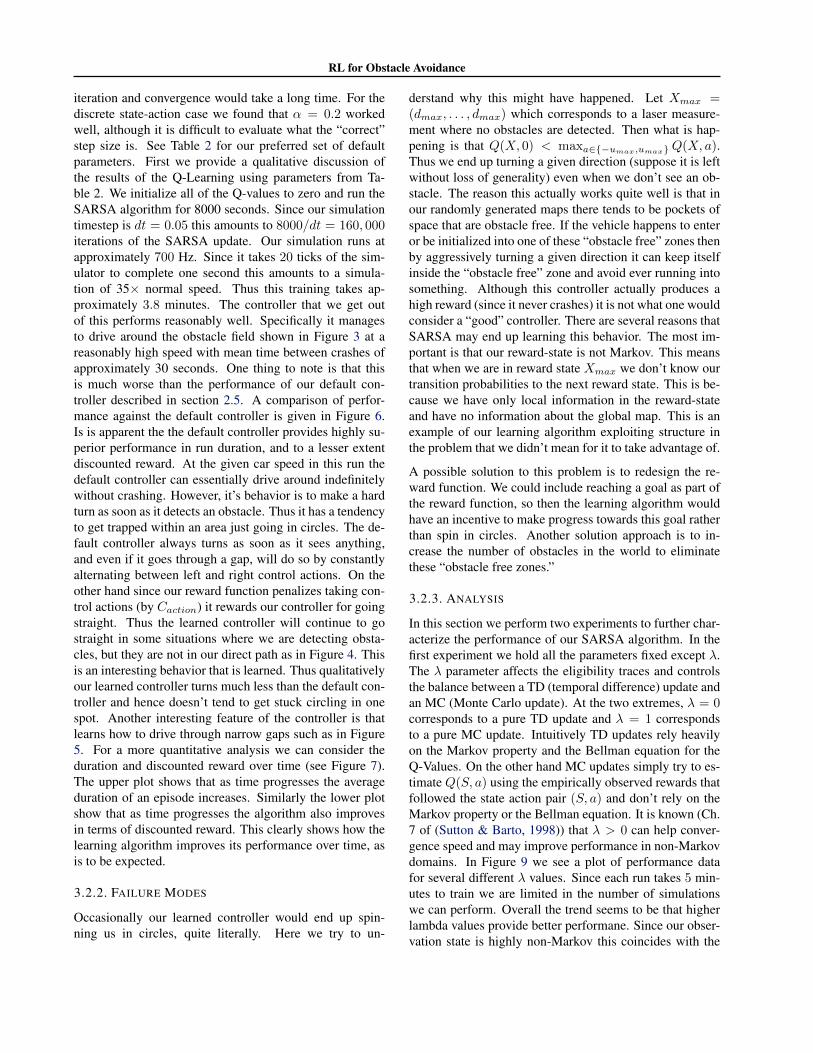
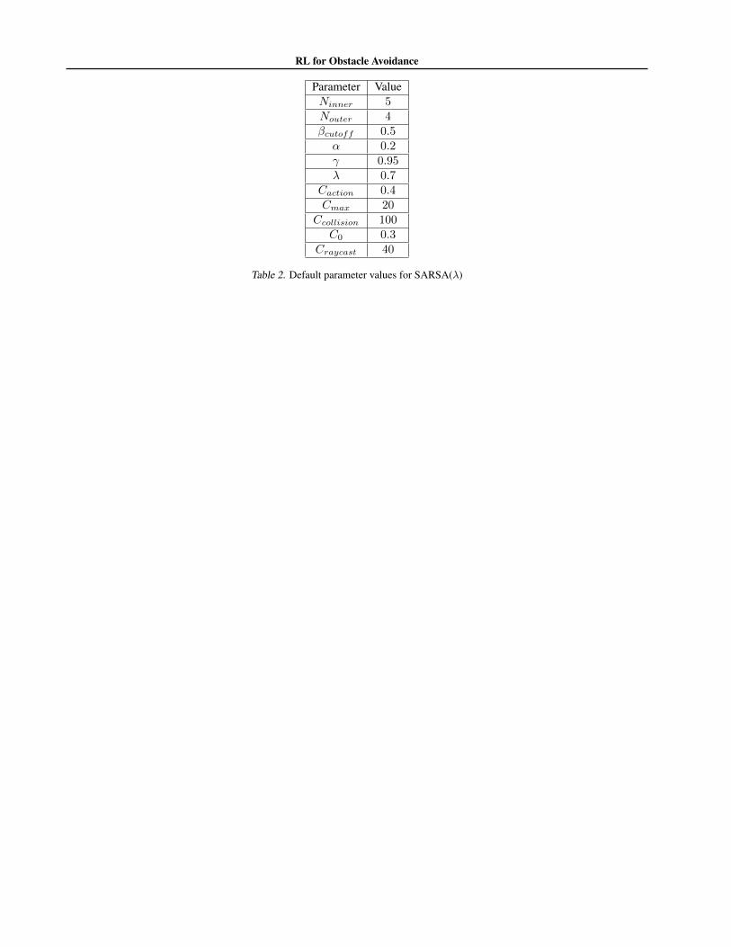
iteration and convergence would take a long time. For thediscrete state-action case we found that ↵ = 0.2 workedwell, although it is difficult to evaluate what the “correct”step size is. See Table 2 for our preferred set of defaultparameters. First we provide a qualitative discussion ofthe results of the Q-Learning using parameters from Ta-ble 2. We initialize all of the Q-values to zero and run theSARSA algorithm for 8000 seconds. Since our simulationtimestep is dt = 0.05 this amounts to 8000/dt = 160, 000

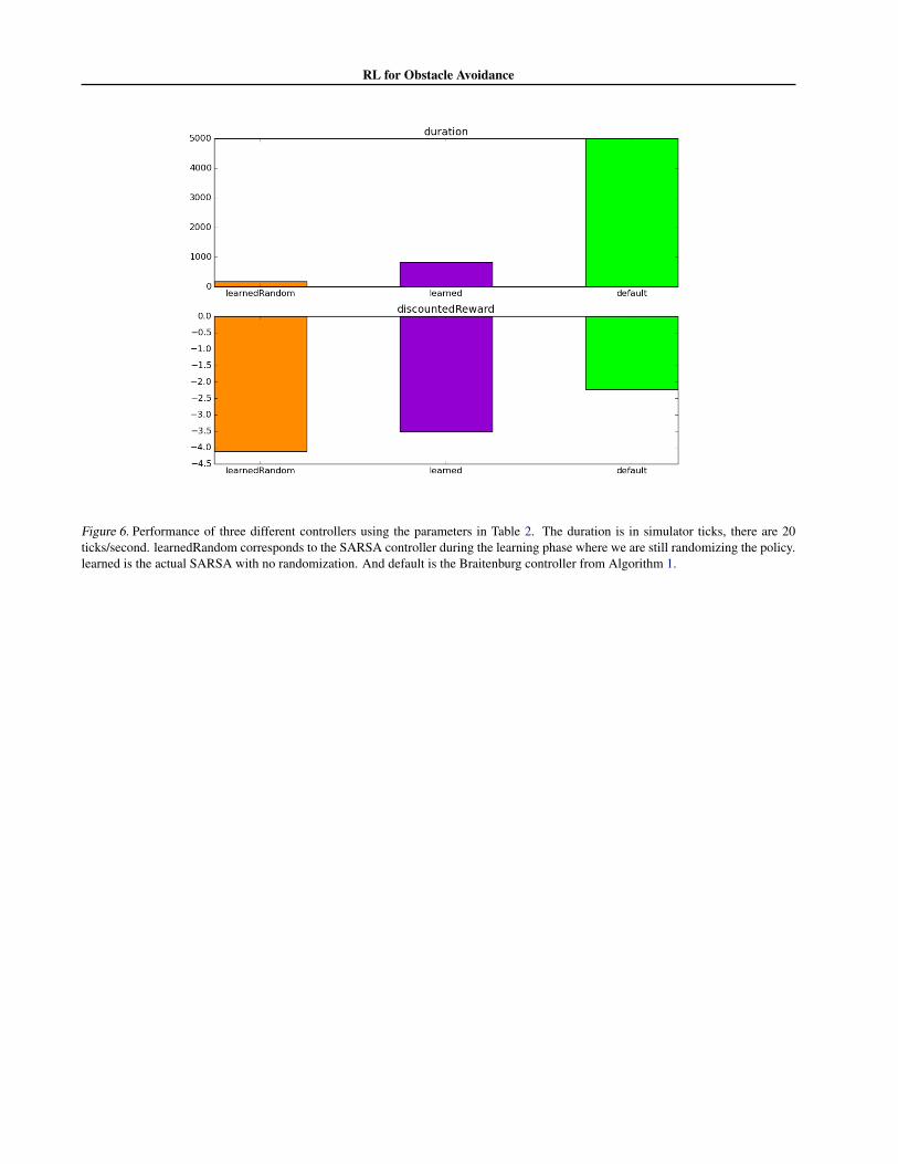
iterations of the SARSA update. Our simulation runs atapproximately 700 Hz. Since it takes 20 ticks of the sim-ulator to complete one second this amounts to a simula-tion of 35⇥ normal speed. Thus this training takes ap-proximately 3.8 minutes. The controller that we get outof this performs reasonably well. Specifically it managesto drive around the obstacle field shown in Figure 3 at areasonably high speed with mean time between crashes ofapproximately 30 seconds. One thing to note is that thisis much worse than the performance of our default con-troller described in section 2.5. A comparison of perfor-mance against the default controller is given in Figure 6.Is is apparent the the default controller provides highly su-perior performance in run duration, and to a lesser extentdiscounted reward. At the given car speed in this run thedefault controller can essentially drive around indefinitelywithout crashing. However, it’s behavior is to make a hardturn as soon as it detects an obstacle. Thus it has a tendencyto get trapped within an area just going in circles. The de-fault controller always turns as soon as it sees anything,and even if it goes through a gap, will do so by constantlyalternating between left and right control actions. On theother hand since our reward function penalizes taking con-trol actions (by C

action

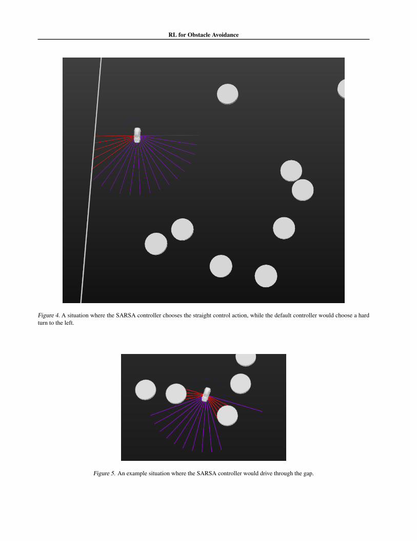
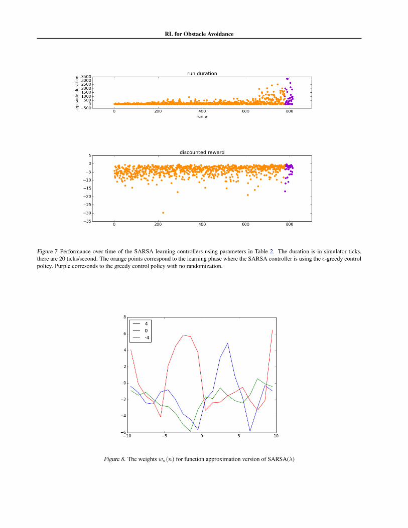
) it rewards our controller for goingstraight. Thus the learned controller will continue to gostraight in some situations where we are detecting obsta-cles, but they are not in our direct path as in Figure 4. Thisis an interesting behavior that is learned. Thus qualitativelyour learned controller turns much less than the default con-troller and hence doesn’t tend to get stuck circling in onespot. Another interesting feature of the controller is thatlearns how to drive through narrow gaps such as in Figure5. For a more quantitative analysis we can consider theduration and discounted reward over time (see Figure 7).The upper plot shows that as time progresses the averageduration of an episode increases. Similarly the lower plotshow that as time progresses the algorithm also improvesin terms of discounted reward. This clearly shows how thelearning algorithm improves its performance over time, asis to be expected.

3.2.2. FAILURE MODES

Occasionally our learned controller would end up spin-ning us in circles, quite literally. Here we try to un-

derstand why this might have happened. Let X

max

=

(d

max

, . . . , d

max

) which corresponds to a laser measure-ment where no obstacles are detected. Then what is hap-pening is that Q(X, 0) < max

a2{�u

max

,u

max

} Q(X, a).Thus we end up turning a given direction (suppose it is leftwithout loss of generality) even when we don’t see an ob-stacle. The reason this actually works quite well is that inour randomly generated maps there tends to be pockets ofspace that are obstacle free. If the vehicle happens to enteror be initialized into one of these “obstacle free” zones thenby aggressively turning a given direction it can keep itselfinside the “obstacle free” zone and avoid ever running intosomething. Although this controller actually produces ahigh reward (since it never crashes) it is not what one wouldconsider a “good” controller. There are several reasons thatSARSA may end up learning this behavior. The most im-portant is that our reward-state is not Markov. This meansthat when we are in reward state X

max

we don’t know ourtransition probabilities to the next reward state. This is be-cause we have only local information in the reward-stateand have no information about the global map. This is anexample of our learning algorithm exploiting structure inthe problem that we didn’t mean for it to take advantage of.

A possible solution to this problem is to redesign the re-ward function. We could include reaching a goal as part ofthe reward function, so then the learning algorithm wouldhave an incentive to make progress towards this goal ratherthan spin in circles. Another solution approach is to in-crease the number of obstacles in the world to eliminatethese “obstacle free zones.”

3.2.3. ANALYSIS

In this section we perform two experiments to further char-acterize the performance of our SARSA algorithm. In thefirst experiment we hold all the parameters fixed except �.The � parameter affects the eligibility traces and controlsthe balance between a TD (temporal difference) update andan MC (Monte Carlo update). At the two extremes, � = 0

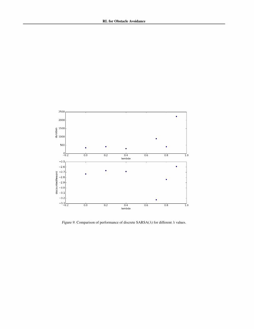
corresponds to a pure TD update and � = 1 correspondsto a pure MC update. Intuitively TD updates rely heavilyon the Markov property and the Bellman equation for theQ-Values. On the other hand MC updates simply try to es-timate Q(S, a) using the empirically observed rewards thatfollowed the state action pair (S, a) and don’t rely on theMarkov property or the Bellman equation. It is known (Ch.7 of (Sutton & Barto, 1998)) that � > 0 can help conver-gence speed and may improve performance in non-Markovdomains. In Figure 9 we see a plot of performance datafor several different � values. Since each run takes 5 min-utes to train we are limited in the number of simulationswe can perform. Overall the trend seems to be that higherlambda values provide better performane. Since our obser-vation state is highly non-Markov this coincides with the


fact that SARSA(�) with � close to 1 is less sensitive toviolations of the Markov property since each update step ismore similar to a MC update.

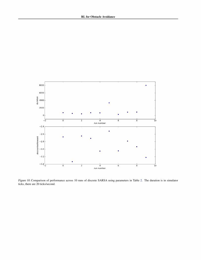
Another interesting fact that we noticed is that, even withthe same set of parameters, different runs of the learningalgorithm can produce quite varied performance. Figure10 shows several runs of the learning algorithm using thesame set of parameters. Out of the 10 trials, runs 5 and 9stand out. They have extremely long average run durationswhich are an order of magnitude larger than all the rest. In-vestigating these runs more carefully they both succumbedto the “drive in circles” failure mode. Thus our learning al-gorithm is sensitive to this failure mode, with about a 20%

failure rate. We believe that with a more carefully designedreward function we could take care of this failure mode.

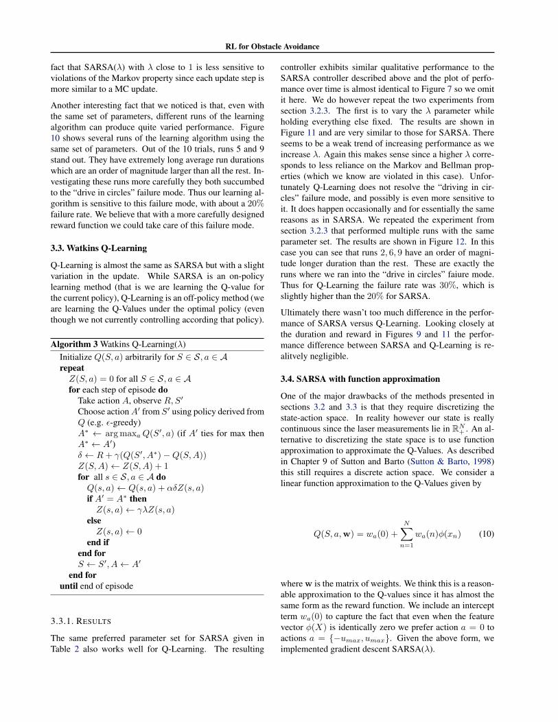
3.3. Watkins Q-Learning

Q-Learning is almost the same as SARSA but with a slightvariation in the update. While SARSA is an on-policylearning method (that is we are learning the Q-value forthe current policy), Q-Learning is an off-policy method (weare learning the Q-Values under the optimal policy (eventhough we not currently controlling according that policy).

Algorithm 3 Watkins Q-Learning(�)Initialize Q(S, a) arbitrarily for S 2 S, a 2 ArepeatZ(S, a) = 0 for all S 2 S, a 2 Afor each step of episode do

Take action A, observe R,S

0

Choose action A

0 from S

0 using policy derived fromQ (e.g. ✏-greedy)A

⇤ argmax

a

Q(S

0, a) (if A0 ties for max then

A

⇤ A

0)� R+ �(Q(S

0, A

⇤)�Q(S,A))

Z(S,A) Z(S,A) + 1

for all s 2 S, a 2 A doQ(s, a) Q(s, a) + ↵�Z(s, a)

if A0= A

⇤ thenZ(s, a) ��Z(s, a)

elseZ(s, a) 0

end ifend forS S

0, A A

0


3.3.1. RESULTS

The same preferred parameter set for SARSA given inTable 2 also works well for Q-Learning. The resulting

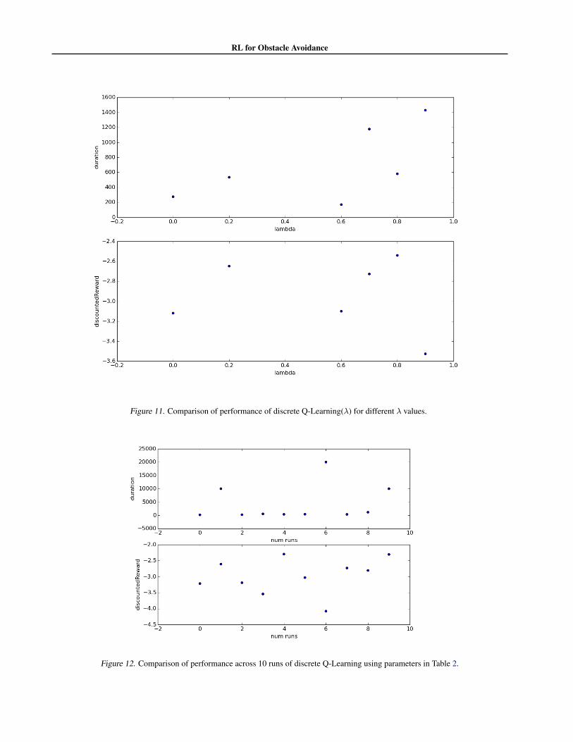
controller exhibits similar qualitative performance to theSARSA controller described above and the plot of perfo-mance over time is almost identical to Figure 7 so we omitit here. We do however repeat the two experiments fromsection 3.2.3. The first is to vary the � parameter whileholding everything else fixed. The results are shown inFigure 11 and are very similar to those for SARSA. Thereseems to be a weak trend of increasing performance as weincrease �. Again this makes sense since a higher � corre-sponds to less reliance on the Markov and Bellman prop-erties (which we know are violated in this case). Unfor-tunately Q-Learning does not resolve the “driving in cir-cles” failure mode, and possibly is even more sensitive toit. It does happen occasionally and for essentially the samereasons as in SARSA. We repeated the experiment fromsection 3.2.3 that performed multiple runs with the sameparameter set. The results are shown in Figure 12. In thiscase you can see that runs 2, 6, 9 have an order of magni-tude longer duration than the rest. These are exactly theruns where we ran into the “drive in circles” faiure mode.Thus for Q-Learning the failure rate was 30%, which isslightly higher than the 20% for SARSA.

Ultimately there wasn’t too much difference in the perfor-mance of SARSA versus Q-Learning. Looking closely atthe duration and reward in Figures 9 and 11 the perfor-mance difference between SARSA and Q-Learning is re-alitvely negligible.

3.4. SARSA with function approximation

One of the major drawbacks of the methods presented insections 3.2 and 3.3 is that they require discretizing thestate-action space. In reality however our state is reallycontinuous since the laser measurements lie in RN

+ . An al-ternative to discretizing the state space is to use functionapproximation to approximate the Q-Values. As describedin Chapter 9 of Sutton and Barto (Sutton & Barto, 1998)this still requires a discrete action space. We consider alinear function approximation to the Q-Values given by

Q(S, a,w) = w

a

(0) +

NX

n=1

w

a

(n)�(x

n

) (10)

where w is the matrix of weights. We think this is a reason-able approximation to the Q-values since it has almost thesame form as the reward function. We include an interceptterm w

a

(0) to capture the fact that even when the featurevector �(X) is identically zero we prefer action a = 0 toactions a = {�u

max

, u

max

}. Given the above form, weimplemented gradient descent SARSA(�).


Algorithm 4 Gradient Descent SARSA(�)Initialize weights w to 0.repeatz = 0

S,A initial state and action of episodefor each step of episode do

Take action A, observe reward R and next state S

0

A

0 policy derived from Q-values at state S

0 (us-ing ✏-greedy)� R+ �Q(S

0, A

0,w)�Q(S,A,w)

wold

ww w + ↵�zz ��z +rwQ(S,A,w

old

)

S S

0, A A

0


Intuitively this corresponds to adjusting the weights wa

(n)

to get the best approximation to the Q-Values in a leastsquares sense (see Button-Sarto Ch. 9 (Sutton & Barto,1998) for a precise statement).

3.4.1. RESULTS

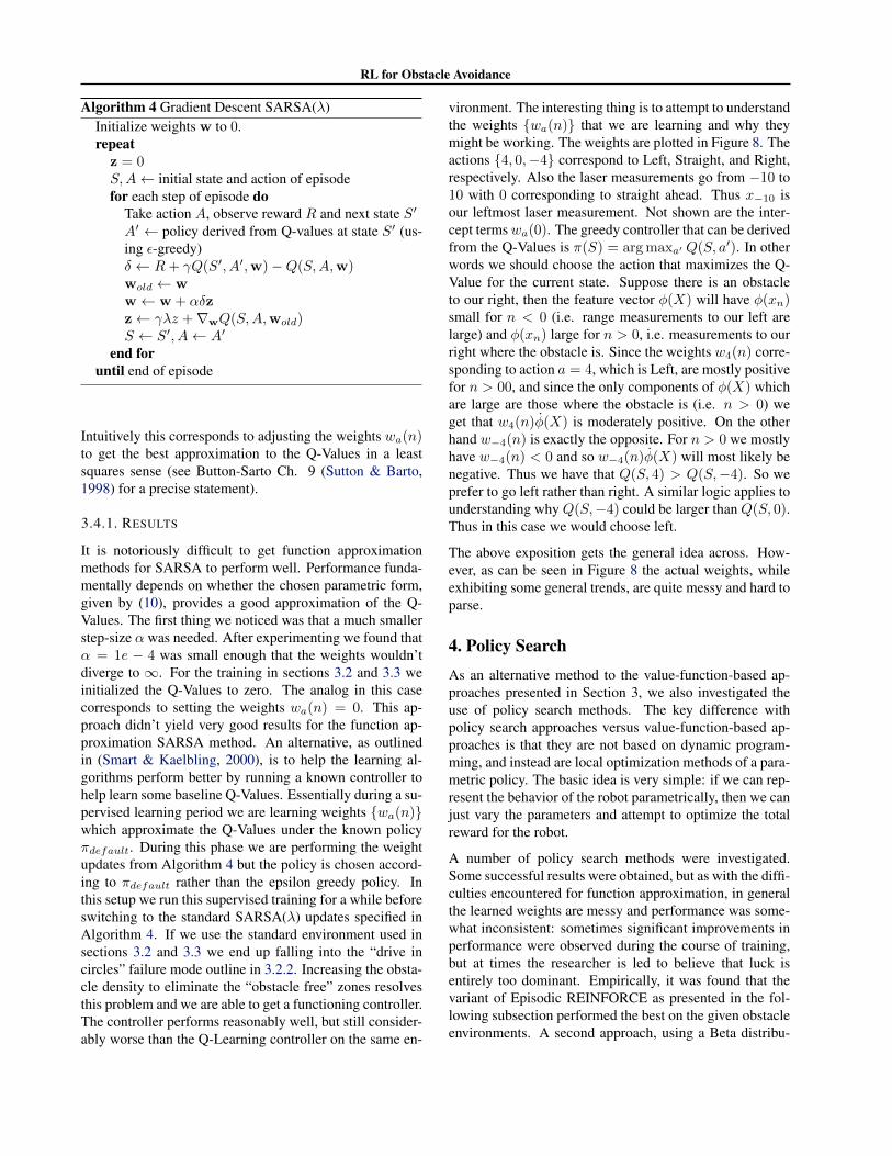
It is notoriously difficult to get function approximationmethods for SARSA to perform well. Performance funda-mentally depends on whether the chosen parametric form,given by (10), provides a good approximation of the Q-Values. The first thing we noticed was that a much smallerstep-size ↵ was needed. After experimenting we found that↵ = 1e � 4 was small enough that the weights wouldn’tdiverge to 1. For the training in sections 3.2 and 3.3 weinitialized the Q-Values to zero. The analog in this casecorresponds to setting the weights w

a

(n) = 0. This ap-proach didn’t yield very good results for the function ap-proximation SARSA method. An alternative, as outlinedin (Smart & Kaelbling, 2000), is to help the learning al-gorithms perform better by running a known controller tohelp learn some baseline Q-Values. Essentially during a su-pervised learning period we are learning weights {w

a

(n)}which approximate the Q-Values under the known policy⇡

default

. During this phase we are performing the weightupdates from Algorithm 4 but the policy is chosen accord-ing to ⇡

default

rather than the epsilon greedy policy. Inthis setup we run this supervised training for a while beforeswitching to the standard SARSA(�) updates specified inAlgorithm 4. If we use the standard environment used insections 3.2 and 3.3 we end up falling into the “drive incircles” failure mode outline in 3.2.2. Increasing the obsta-cle density to eliminate the “obstacle free” zones resolvesthis problem and we are able to get a functioning controller.The controller performs reasonably well, but still consider-ably worse than the Q-Learning controller on the same en-

vironment. The interesting thing is to attempt to understandthe weights {w

a

(n)} that we are learning and why theymight be working. The weights are plotted in Figure 8. Theactions {4, 0,�4} correspond to Left, Straight, and Right,respectively. Also the laser measurements go from �10 to10 with 0 corresponding to straight ahead. Thus x�10 isour leftmost laser measurement. Not shown are the inter-cept terms w

a

(0). The greedy controller that can be derivedfrom the Q-Values is ⇡(S) = argmax

a

0Q(S, a

0). In other

words we should choose the action that maximizes the Q-Value for the current state. Suppose there is an obstacleto our right, then the feature vector �(X) will have �(x

n

)

small for n < 0 (i.e. range measurements to our left arelarge) and �(x

n

) large for n > 0, i.e. measurements to ourright where the obstacle is. Since the weights w4(n) corre-sponding to action a = 4, which is Left, are mostly positivefor n > 00, and since the only components of �(X) whichare large are those where the obstacle is (i.e. n > 0) weget that w4(n)

˙

�(X) is moderately positive. On the otherhand w�4(n) is exactly the opposite. For n > 0 we mostlyhave w�4(n) < 0 and so w�4(n)

˙

�(X) will most likely benegative. Thus we have that Q(S, 4) > Q(S,�4). So weprefer to go left rather than right. A similar logic applies tounderstanding why Q(S,�4) could be larger than Q(S, 0).Thus in this case we would choose left.

The above exposition gets the general idea across. How-ever, as can be seen in Figure 8 the actual weights, whileexhibiting some general trends, are quite messy and hard toparse.

4. Policy SearchAs an alternative method to the value-function-based ap-proaches presented in Section 3, we also investigated theuse of policy search methods. The key difference withpolicy search approaches versus value-function-based ap-proaches is that they are not based on dynamic program-ming, and instead are local optimization methods of a para-metric policy. The basic idea is very simple: if we can rep-resent the behavior of the robot parametrically, then we canjust vary the parameters and attempt to optimize the totalreward for the robot.

A number of policy search methods were investigated.Some successful results were obtained, but as with the diffi-culties encountered for function approximation, in generalthe learned weights are messy and performance was some-what inconsistent: sometimes significant improvements inperformance were observed during the course of training,but at times the researcher is led to believe that luck isentirely too dominant. Empirically, it was found that thevariant of Episodic REINFORCE as presented in the fol-lowing subsection performed the best on the given obstacleenvironments. A second approach, using a Beta distribu-


tion, is discussed as well, and although it did not produceuniversally successful obstacle avoidance maneuvers, it isnonetheless interesting to analyze.

It is interesting to note the list of differences with the meth-ods of the last section. For one, policy search is able to han-dle continuous state and action spaces without discretiza-tion. The function approximation approach discussed inSection 3.4 is able to consume a continuous state space,but still is limited to a discrete action space, whereas policysearch methods may be continuous in both. Also in contrastwith the dynamic programming methods, these gradient-descent-based policy search methods are inherently localsearch, and so we have no guarantees on finding globalmaxima even if we had access to a full Markov state. Themethods investigated all used at least 10 parameters, and soit is very likely that local maxima were abundant in thesehigh-dimensional spaces. Stochasticity in gradient descentmay have contributed to escaping local maxima, but it isdifficult to say. It is also useful to note that the policy searchmethods discussed were all episodic in nature – i.e., therewas no TD (temporal difference) analog used here for pol-icy search. Although such methods exist, it was easier ininitial investigations to focus on the episodic versions.

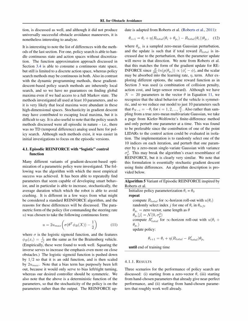
4.1. Episodic REINFORCE with “logistic” controlfunction

Many different variants of gradient-descent-based opti-mization of a parametric policy were investigated. The fol-lowing was the algorithm with which the most empiricalsuccess was achieved. It has been able to repeatedly findparameters that seem capable of developing smart behav-ior, and in particular is able to increase, stochastically, theaverage duration which which the robot is able to avoidcrashing. It is different in a few ways from what mightbe considered a standard REINFORCE algorithm, and thereasons for these differences will be discussed. The para-metric form of the policy (for commanding the steering rateu) was chosen to take the following continuous form:

u = 2u

max

✓�(✓

T

�

B

(X))� 1

2

◆(11)

where � is the logistic sigmoid function, and the features�

B

(x

i

) =

1x

2i

are the same as for the Braitenberg vehicle.(Empirically, these were found to work well. Squaring theinverse serves to increase the emphasis even more on closeobstacles.) The logistic sigmoid function is pushed downby 1/2 so that it is an odd function, and is then scaledby 2u

max

. Note that a bias term has purposely been leftout, because it would only serve to bias left/right turning,whereas our desired controller should be symmetric. Wealso note that the above is a deterministic function of theparameters, so that the stochasticity of the policy is on theparameters rather than the output. The REINFORCE up-

date is adapted from Roberts et al. (Roberts et al., 2011):

✓

i+1 = ✓

i

+ ⌘(R

total

(✓

i

+ ✓

p

i

)�R

total

(✓

i

))✓

p

i

, (12)

where ✓

p

i

is a sampled zero-mean Gaussian perturbation,and the update is such that if total reward R

total

is in-creased due to the perturbation, then the parameter updatewill move in that direction. We note from Roberts et al.that this matches the form of the gradient update for RE-INFORCE since @

@✓

i

ln(p(✓

p

i

)) / (�

0i

� �), and the scalarmay be absorbed into the learning rate, ⌘, term. After ex-ploring different options, the same reward function as inSection 3 was used (a combination of collision penalty,action cost, and large-sensor reward). Although we haveN = 20 parameters in the vector ✓ in Equation 11, werecognize that the ideal behavior of the vehicle is symmet-ric, and so we reduce our model to just 10 parameters suchthat ✓

N�i

= �✓i

for i = 1, 2, ...,

N

2 . Also rather than sam-pling from a true zero-mean multivariate Gaussian, we takea page from Kiefer-Wolfowitz’s finite-difference methodand only perturb one parameter at a time. This was foundto be preferable since the contribution of one of the pointLIDARs to the control action could be evaluated in isola-tion. The implementation is to randomly select one of the10 indices on each iteration, and perturb that one param-eter by a zero-mean single-variate Gaussian with variance�

2p

. This may break the algorithm’s exact resemblance ofREINFORCE, but it is clearly very similar. We note thatthis formulation is essentially stochastic gradient descentusing finite differences. An algorithm description is pro-vided below.

Algorithm 5 Variant of Episodic REINFORCE inspired byRoberts et al.

Initialize policy parameterization ✓

i

= ✓0

repeatcompute R

total

for1-horizon roll-out with u(✓

i

)

randomly select index j for one of ✓i

in ✓

left

✓

p

i

= zero vector, same length as ✓✓

p

i

[j] = N (0,�

2p

)

compute R

0total

for 1-horizon roll-out with u(✓

i

+

✓

p

i

)

update policy:

✓

i+1 = ✓

i

+ ⌘(R

total

�R

0total

)✓

p

i

until end of training time

4.1.1. RESULTS

Three scenarios for the performance of policy search arediscussed: (i) starting from a zero-vector ✓, (iii) startingfrom hand-chosen parameters that already give near-perfectperformance, and (ii) starting from hand-chosen parame-ters that roughly work well already.


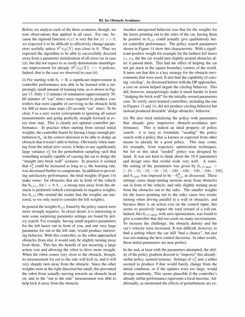
Before we analyze each of the three scenarios, though, wenote observations that applied in all cases. For one, be-cause the sigmoid function �(x) is very flat for |x| >> 0,we expected it to be difficult to effectively change param-eters usefully unless ✓

T

�

B

(X) was close to 0. Thus weexpected the algorithm to be able to successfully descendaway from a parameter initialization of all zeros (as in case(i)), but did not expect to as easily demonstrate unambigu-ous improvement for already |✓T�

B

(X)| >> 0 policies.Indeed, that is the case we observed in case (ii).

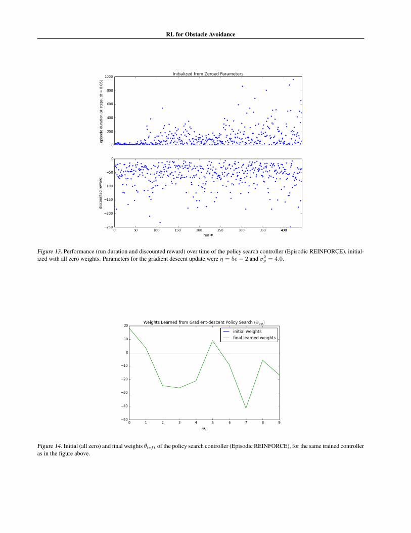
(i) For starting with ✓0 = 0, a significant improvement incontroller performance was able to be learned with a sur-prisingly small amount of training time, as is shown in Fig-ure 13. Only 1-2 minutes of simulation (approximately 30-60 minutes of “car” time) were required to produce con-trollers that were capable of surviving in the obstacle fieldfor 400 or more time steps (20 seconds “car” time). To beclear, ✓ as a zero vector corresponds to ignoring all sensormeasurements and going perfectly straight forward at ev-ery time step. This is clearly not optimal controller per-formance. In practice when starting from zeroed initialweights, the controller learns by having a large enough per-turbation ✓

p

i

in the correct direction to be able to dodge anobstacle that it wasn’t able to before. Obviously when start-ing from the initial zero vector, it helps to use significantlylarge variance �

2p

for the perturbation sampling such thatsomething actually capable of causing the car to dodge the“straight into brick wall” scenario. In practice it seemedthat �2

p

could be increased as long as ⌘, the learning rate,was decreased further to compensate. In addition to provid-ing satisfactory performance, the final weights (Figure 14)make sense: for obstacles that are in front of the vehiclethe ✓

left,i

for i = 9, 8, .., a strong turn away from the ob-stacle is preferred (which corresponds to negative weights,for ✓

left

(We remind the reader that the weights are mir-rored, so we only need to consider the left weights).

In general the weights ✓left

found by the policy search weremore strongly negative. In closer detail, it is interesting tonote some surprising parameter settings are found by pol-icy search. For example. having small negative parametersfor the left lasers out in front of you, and one very largeparameter for out to the left side, would produce interest-ing behavior. With this controller, as the robot approachedobstacles from afar, it would only be slightly turning awayfrom them. This has the benefit of not incurring a largeaction cost and allowing the robot to drive more straight.When the robot comes very close to the obstacle, though,its measurement for out to the side will kick in, and it willvery sharply turn away from the obstacle. Since the otherweights were in the right direction but small, this preventedthe robot from actually moving towards an obstacle headon, and so the “out to the side” measurement was able tohelp kick it away from the obstacle.

Another unexpected behavior was that for the weights forthe lasers pointing out to the sides of the car, having thembe positive in ✓

left

could actually give qualitatively bet-ter controller performance. The policy search parametersshown in Figure 14 show this characteristic. With a signif-icant positive weight for example for the farthest left lasersx1, x2, the the car would turn slightly around obstacles af-ter it passed them. This had the effect of helping the carnot get stuck in the square boundary corners of the world.It turns out that this is a key strategy for the obstacle envi-ronments that were used. It also had the capability of caus-ing ‘circling’. As discussed before with the DP approaches,a cost on action helped negate the circling behavior. Thisdid, however, unsurprisingly make it much harder to learn“dodging the brick wall” for the initially-zeroed parameterscase. To verify, most learned controllers, including the onein Figures 13 and 14, did not produce circling behavior butinstead produced desirable ‘dodge obstacles’ behavior.

(ii) We also tried initializing the policy with parametersthat already gave impressive obstacle-avoidance per-formance. This is indeed an ideal property of policysearch: it is easy to formulate “seeding” the policysearch with a policy that is known or expected from othermeans to already be a good policy. This may come,for example, from trajectory optimization techniques,but for us this ideal “seeded” policy was designed byhand. It was not hard to think about the 10 ✓ parametersand design ones that would work very well. A sensi-ble setting of the parameters was given by ✓

left,ideal =

[�10,�10,�10,�10,�10,�100,�100,�100,�100,�100],and ✓

right

was imposed to be �✓Rleft

as discussed. Thesesettings cause sharp turning motions away from obstaclesout in front of the vehicle, and only slightly turning awayfrom the obstacles out to the sides. The smaller weightsfor the lasers pointing out to the sides cause less erraticturning when driving parallel to a wall or obstacles, andbecause there is an action cost on the control input, thisseems to positively impact the total reward of a roll-out.Indeed, this ✓

left,ideal, with zero optimization, was found togive a controller that did not crash on many environments.To increase the challenge, the obstacle density and thecar’s velocity were increased. It was difficult, however, tofind a setting where the car still “had a chance”, but justwas not making the best control decisions. In other words,these initial parameters are near perfect.

In the end, at least with the parameters attempted, the abil-ity of the policy gradient descent to “improve” this already-stellar policy seemed tenuous. Settings of �2

p

and ⌘ eitherseemed to produce ✓ that would barely change from theinitial condition, or if the updates were too large, woulddiverge randomly. This seems plausible if the controller’salready stellar performance represents a local maxima. Ad-ditionally, as mentioned the effects of perturbations are ex-


pected to be small when the input to the sigmoid alreadycontains values far from zero, as is the case with these largeinitial parameters. It is possible that this is primarily a re-sult of using the sigmoid function. In short, if the policyis already really good, then policy search may not surpris-ingly have a difficult job of improving performance.

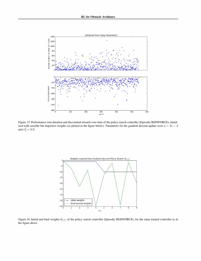
(iii) Finally, we investigate a third scenario, wherethe initial parameters are not stellar, but they arealso not zero. For this purpose, ✓

left,okay =

[�1,�1,�1,�1,�1,�10,�10,�10,�10,�10] sufficed.This is similar to the parameters just discussed, but withless strong turning. In this case, the policy gradient descentwas able to find improved parameterizations, as shown inFigure 15, although of course the increase in performancewas not as drastic as it was for the zeroed initial parame-ters. The parameters found by policy search (Figure 16)were sensibly more negative than the initial parameters.It is interesting to note that although the weights appearto be very “noisy” from ✓

i

to ✓

i+1, if we think aboutthis, it is not too surprising. Having a sequence of threeweights be [�10,�40,�10] is not all that different from[�20,�20,�20] since in these obstacle environments, ifone laser is intersecting an obstacle, then the chances arethat its neighbor is as well.

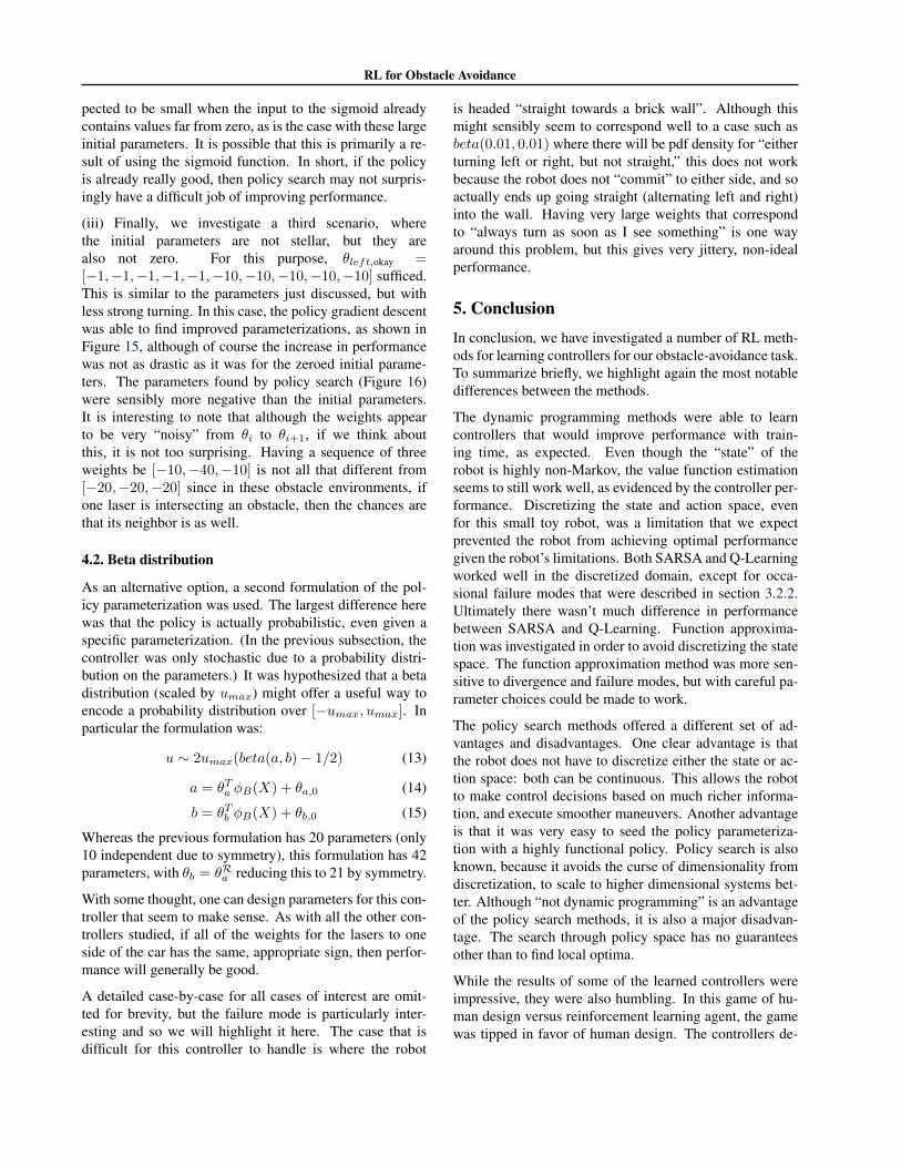
4.2. Beta distribution

As an alternative option, a second formulation of the pol-icy parameterization was used. The largest difference herewas that the policy is actually probabilistic, even given aspecific parameterization. (In the previous subsection, thecontroller was only stochastic due to a probability distri-bution on the parameters.) It was hypothesized that a betadistribution (scaled by u

max

) might offer a useful way toencode a probability distribution over [�u

max

, u

max

]. Inparticular the formulation was:

u ⇠ 2u

max

(beta(a, b)� 1/2) (13)

a = ✓

T

a

�

B

(X) + ✓

a,0 (14)

b = ✓

T

b

�

B

(X) + ✓

b,0 (15)

Whereas the previous formulation has 20 parameters (only10 independent due to symmetry), this formulation has 42parameters, with ✓

b

= ✓

Ra

reducing this to 21 by symmetry.

With some thought, one can design parameters for this con-troller that seem to make sense. As with all the other con-trollers studied, if all of the weights for the lasers to oneside of the car has the same, appropriate sign, then perfor-mance will generally be good.

A detailed case-by-case for all cases of interest are omit-ted for brevity, but the failure mode is particularly inter-esting and so we will highlight it here. The case that isdifficult for this controller to handle is where the robot

is headed “straight towards a brick wall”. Although thismight sensibly seem to correspond well to a case such asbeta(0.01, 0.01) where there will be pdf density for “eitherturning left or right, but not straight,” this does not workbecause the robot does not “commit” to either side, and soactually ends up going straight (alternating left and right)into the wall. Having very large weights that correspondto “always turn as soon as I see something” is one wayaround this problem, but this gives very jittery, non-idealperformance.

5. ConclusionIn conclusion, we have investigated a number of RL meth-ods for learning controllers for our obstacle-avoidance task.To summarize briefly, we highlight again the most notabledifferences between the methods.

The dynamic programming methods were able to learncontrollers that would improve performance with train-ing time, as expected. Even though the “state” of therobot is highly non-Markov, the value function estimationseems to still work well, as evidenced by the controller per-formance. Discretizing the state and action space, evenfor this small toy robot, was a limitation that we expectprevented the robot from achieving optimal performancegiven the robot’s limitations. Both SARSA and Q-Learningworked well in the discretized domain, except for occa-sional failure modes that were described in section 3.2.2.Ultimately there wasn’t much difference in performancebetween SARSA and Q-Learning. Function approxima-tion was investigated in order to avoid discretizing the statespace. The function approximation method was more sen-sitive to divergence and failure modes, but with careful pa-rameter choices could be made to work.

The policy search methods offered a different set of ad-vantages and disadvantages. One clear advantage is thatthe robot does not have to discretize either the state or ac-tion space: both can be continuous. This allows the robotto make control decisions based on much richer informa-tion, and execute smoother maneuvers. Another advantageis that it was very easy to seed the policy parameteriza-tion with a highly functional policy. Policy search is alsoknown, because it avoids the curse of dimensionality fromdiscretization, to scale to higher dimensional systems bet-ter. Although “not dynamic programming” is an advantageof the policy search methods, it is also a major disadvan-tage. The search through policy space has no guaranteesother than to find local optima.

While the results of some of the learned controllers wereimpressive, they were also humbling. In this game of hu-man design versus reinforcement learning agent, the gamewas tipped in favor of human design. The controllers de-


signed by hand worked significantly better with signifi-cantly less effort: the value function controllers were notable to beat the performance of the Braitenberg controller,and the policy search did not significantly improve upon aparameterization that was chosen by design in a couple ofminutes.

In theory there seems to be no reason, for example, thatgiven sufficiently small step sizes, and sufficient randominitializations, that a policy search method can’t verifiablyimprove the performance of a hand-designed parameteriza-tion. In practice, though, this is not that easy!

6. Division of LaborLucas implemented the value function based controllers(SARSA, and Q-Learning, both discrete and function ap-proximation). He also helped build out the simulation en-vironment, and wrote the utility methods for logging, play-back and plot generation. Pete built out the library ofobject-oriented modules and pulled together the simulationenvironment, designed the Braitenberg controllers, and im-plemented the policy search methods. The overall simula-tion architecture was designed together.

7. AcknowledgementsThe authors would like to thank Professor Leslie Kaelblingfor her enthusiasm, for helping us with ideas, and for sup-porting us in developing the project. We also thank PatMarion for his great help in developing the visualizationenvironment.

ReferencesMarion, Pat. Director: A robotics interface and visualiza-

tion framework, 2015. URL http://github.com/

RobotLocomotion/director.

Roberts, John, Manchester, Ian, and Tedrake, Russ.Feedback controller parameterizations for reinforcementlearning. In 2011 IEEE Symposium on Adaptive Dy-

namic Programming and Reinforcement Learning (AD-

PRL), 2011.

Smart, William D. and Kaelbling, Leslie Pack. Practicalreinforcement learning in continuous spaces. pp. 903–910. Morgan Kaufmann, 2000.

Sutton, R.S. and Barto, A.G. Reinforcement learning: An

introduction. Cambridge Univ Press, 1998.

http://github.com/RobotLocomotion/director

http://github.com/RobotLocomotion/director


Figure 2. The weights W for computing the reward.

Figure 3. The obstacle field used for the majority of the learning runs


Figure 4. A situation where the SARSA controller chooses the straight control action, while the default controller would choose a hardturn to the left.

Figure 5. An example situation where the SARSA controller would drive through the gap.


Figure 6. Performance of three different controllers using the parameters in Table 2. The duration is in simulator ticks, there are 20ticks/second. learnedRandom corresponds to the SARSA controller during the learning phase where we are still randomizing the policy.learned is the actual SARSA with no randomization. And default is the Braitenburg controller from Algorithm 1.


Figure 7. Performance over time of the SARSA learning controllers using parameters in Table 2. The duration is in simulator ticks,there are 20 ticks/second. The orange points correspond to the learning phase where the SARSA controller is using the ✏-greedy controlpolicy. Purple corresonds to the greedy control policy with no randomization.

Figure 8. The weights wa(n) for function approximation version of SARSA(�)


Figure 9. Comparison of performance of discrete SARSA(�) for different � values.


Figure 10. Comparison of performance across 10 runs of discrete SARSA using parameters in Table 2. The duration is in simulatorticks, there are 20 ticks/second.


Figure 11. Comparison of performance of discrete Q-Learning(�) for different � values.

Figure 12. Comparison of performance across 10 runs of discrete Q-Learning using parameters in Table 2.


Figure 13. Performance (run duration and discounted reward) over time of the policy search controller (Episodic REINFORCE), initial-ized with all zero weights. Parameters for the gradient descent update were ⌘ = 5e� 2 and �2

p = 4.0.

Figure 14. Initial (all zero) and final weights ✓left of the policy search controller (Episodic REINFORCE), for the same trained controlleras in the figure above.


Figure 15. Performance (run duration and discounted reward) over time of the policy search controller (Episodic REINFORCE), initial-ized with sensible but imperfect weights (as plotted in the figure below). Parameters for the gradient descent update were ⌘ = 2e � 2and �2

p = 6.0.

Figure 16. Initial and final weights ✓left of the policy search controller (Episodic REINFORCE), for the same trained controller as inthe figure above.


Parameter ValueN

inner

5

N

outer

4

�

cutoff

0.5

↵ 0.2

� 0.95

� 0.7

C

action

0.4

C

max

20

C

collision

100

C0 0.3

C

raycast

40

Table 2. Default parameter values for SARSA(�)

reinforcement learning for autonomous driving obstacle ... · reinforcement learning for autonomous...

Documents