regularization methods for sdp relaxations …njw/publicpapers/regpop.pdf · regularization methods...
TRANSCRIPT

REGULARIZATION METHODS FOR SDP RELAXATIONS INLARGE SCALE POLYNOMIAL OPTIMIZATION
JIAWANG NIE∗ AND LI WANG∗
Abstract. We study how to solve semidefinite programming (SDP) relaxations for large scalepolynomial optimization. When interior-point methods are used, typically only small or moderatelylarge problems could be solved. This paper studies regularization methods for solving polynomialoptimization problems. We describe these methods for semidefinite optimization with block struc-tures, and then apply them to solve large scale polynomial optimization problems. The performanceis tested on various numerical examples. By regularization methods, significantly bigger problemscould be solved on a regular computer, which is almost impossible by interior point methods.
Key words. polynomial optimization, Lasserre’s relaxation, regularization methods, semidefi-nite programming, sum of squares
AMS subject classifications. 65K05, 90C22
1. Introduction. Consider the polynomial optimization problem
(1.1) minx∈Rn
f(x) s.t. x ∈ S
where f(x) is a multivariate polynomial and S ⊆ Rn is a semialgebraic set (definedby a boolean combination of polynomial equalities or inequalities). Recently, therehas been much work on solving (1.1) by semidefinite programming (SDP) relaxation(also called Lasserre’s relaxation in the literature). The basic idea is approximatingnonnegative polynomials by sum of squares (SOS) type polynomials, which is equiv-alent to solving some SDP problems. Thus, the SDP packages (like SDPT3 [26],SeDuMi [25], SDPA[8]) would be applied to solve polynomial optimization problems.Typically, SDP relaxation is very successful in solving (1.1), as demonstrated by thepioneer work of Lasserre [14], Parrilo and Sturmfels [20] and many others. However,their applications are very limited in solving big problems. For instance, to minimizea general quartic polynomial, it is almost impossible to solve its SDP relaxation ona regular computer when it has more than 30 variables. So far, SDP relaxations forpolynomial optimization can only be solved for small or moderately large problems,which severely limits their practical applications. Bigger problems would be solvedif sparsity is exploited, like in the work [18, 27]. The motivation of this paper isproposing new methods for solving large scale SDP relaxations arising from generalpolynomial optimization.
A standard SDP problem is
(1.2) minX∈SN
C •X s.t. A(X) = b, X º 0.
Here SN denotes the space of N ×N real symmetric matrices, X º 0 (resp. X Â 0)meansX is positive semidefinite (resp. definite), and • denotes the standard Frobeniusinner product. The C ∈ SN and b ∈ Rm are constant, and A : SN → Rm is a linearoperator. The dual problem of (1.2) is
(1.3) max bT y s.t. A∗(y) + Z = C, Z º 0.
∗Department of Mathematics, University of California, 9500 Gilman Drive, La Jolla, CA 92093.Emails: [email protected], [email protected]. The research was partially supported by NSFgrants DMS-0757212 and DMS-0844775.
1
2 Jiawang Nie and Li Wang
Here A∗ is the adjoint of A. An X is optimal for (1.2) and (y, Z) is optimal for (1.3)if the triple (X, y, Z) satisfies the optimality condition
(1.4)A(X) = b
A∗(y) + Z = CX,Z º 0, XZ = 0
.
There is much work on solving SDP by interior point methods. We refer to [28]for theory and algorithms for SDP. Most of them generate a sequence {(Xk, yk, Zk)}converging to an optimal triple. At each step, a search direction (∆X,∆y,∆Z) needsto be computed. To compute ∆y, typically an m×m linear system needs to be solved.To compute ∆X and ∆Z, two linear matrix equations need to be solved. The cost forcomputing ∆y is O(m3). When m = O(N), the cost for computing ∆y is O(N3). Inthis case, solving SDP is not very expensive if N is not too big (like less than 1, 000).However, when m = O(N2), the cost for computing ∆y would be O(N6), which isvery expensive even for moderately large N (like 500). In this case, computing ∆yis very expensive. It requires storing a matrix of dimension m ×m in computer andO(m3) arithmetic operations.
Unfortunately, SDP relaxations arising from polynomial optimization belong tothe bad case that m = O(N2), which is why the SDP solvers based on interior pointmethods have difficulty in solving big polynomial optimization problems (like degree4 with 100 variables). We explain why this is the case. Let p(x) be a polynomialof degree 2d. Then, p(x) is SOS if and only if there exists X º 0 such that p(x) =[x]Td X[x]d (cf. [21]), where
[x]Td := [ 1 x1 · · · xn x21 x1x2 · · · · · · xd
1 xd−11 x2 · · · · · · xd
n ].
Note the length of [x]d is N =(n+dd
). If we write
p(x) =∑
α∈Nn:|α|≤2d
pαxα11 · · ·xαn
n ,
then p(x) being SOS is equivalent to the existence of a symmetric N ×N matrix Xsatisfying
(1.5)Aα •X = pα ∀α ∈ Nn : |α| ≤ 2d,
X º 0.
}
Here Aα are certain constant symmetric matrices. The number of equalities is m =(n+2d2d
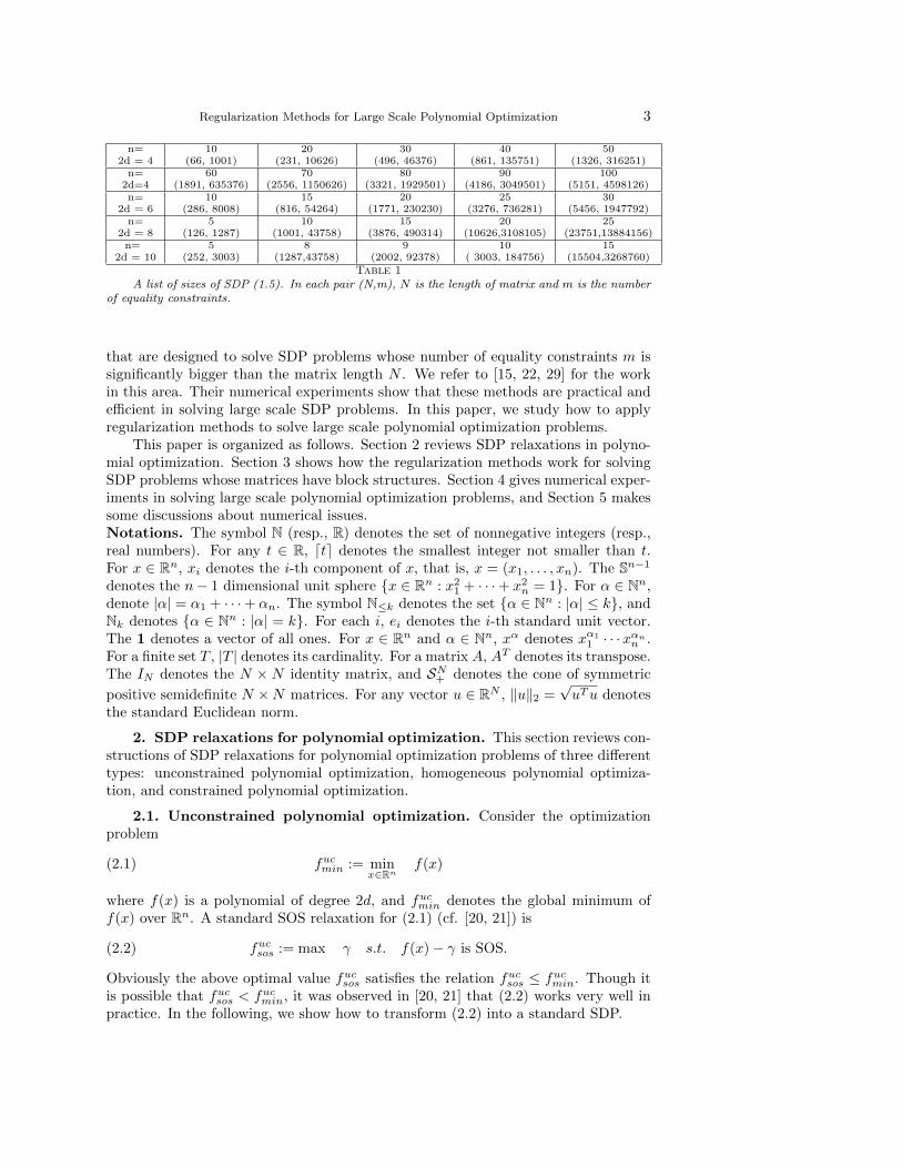
). For any fixed d, m = O(n2d) = O(N2). The size of SDP (1.5) is huge for
moderately large n and d. Table 1 lists the size of SDP (1.5) for some typical valuesof (n, 2d). As we have seen earlier, when interior point methods are applied to solve(1.2)-(1.3), at each step we need to solve a linear system and two matrix equations.To compute ∆y, we need to store an m×m matrix and implement O(n6d) arithmeticoperations. This is very expensive for even moderately large n and d, and henceseverely limits the solvability of SDP relaxations in polynomial optimization. Forinstance, on a regular computer, to solve a general quartic polynomial optimizationproblem, it is almost impossible to apply interior point methods when there are morethan 30 variables.
Recently, there has been much work on designing efficient numerical methodson solving big SDP problems. Regularization methods are such a kind of algorithms
Regularization Methods for Large Scale Polynomial Optimization 3
n= 10 20 30 40 502d = 4 (66, 1001) (231, 10626) (496, 46376) (861, 135751) (1326, 316251)n= 60 70 80 90 100
2d=4 (1891, 635376) (2556, 1150626) (3321, 1929501) (4186, 3049501) (5151, 4598126)n= 10 15 20 25 30
2d = 6 (286, 8008) (816, 54264) (1771, 230230) (3276, 736281) (5456, 1947792)n= 5 10 15 20 25
2d = 8 (126, 1287) (1001, 43758) (3876, 490314) (10626,3108105) (23751,13884156)n= 5 8 9 10 15
2d = 10 (252, 3003) (1287,43758) (2002, 92378) ( 3003, 184756) (15504,3268760)
Table 1A list of sizes of SDP (1.5). In each pair (N,m), N is the length of matrix and m is the number
of equality constraints.
that are designed to solve SDP problems whose number of equality constraints m issignificantly bigger than the matrix length N . We refer to [15, 22, 29] for the workin this area. Their numerical experiments show that these methods are practical andefficient in solving large scale SDP problems. In this paper, we study how to applyregularization methods to solve large scale polynomial optimization problems.
This paper is organized as follows. Section 2 reviews SDP relaxations in polyno-mial optimization. Section 3 shows how the regularization methods work for solvingSDP problems whose matrices have block structures. Section 4 gives numerical exper-iments in solving large scale polynomial optimization problems, and Section 5 makessome discussions about numerical issues.Notations. The symbol N (resp., R) denotes the set of nonnegative integers (resp.,real numbers). For any t ∈ R, dte denotes the smallest integer not smaller than t.For x ∈ Rn, xi denotes the i-th component of x, that is, x = (x1, . . . , xn). The Sn−1
denotes the n− 1 dimensional unit sphere {x ∈ Rn : x21 + · · ·+ x2
n = 1}. For α ∈ Nn,denote |α| = α1 + · · ·+ αn. The symbol N≤k denotes the set {α ∈ Nn : |α| ≤ k}, andNk denotes {α ∈ Nn : |α| = k}. For each i, ei denotes the i-th standard unit vector.The 1 denotes a vector of all ones. For x ∈ Rn and α ∈ Nn, xα denotes xα1
1 · · ·xαnn .
For a finite set T , |T | denotes its cardinality. For a matrix A, AT denotes its transpose.The IN denotes the N × N identity matrix, and SN
+ denotes the cone of symmetric
positive semidefinite N ×N matrices. For any vector u ∈ RN , ‖u‖2 =√uTu denotes
the standard Euclidean norm.
2. SDP relaxations for polynomial optimization. This section reviews con-structions of SDP relaxations for polynomial optimization problems of three differenttypes: unconstrained polynomial optimization, homogeneous polynomial optimiza-tion, and constrained polynomial optimization.
2.1. Unconstrained polynomial optimization. Consider the optimizationproblem
(2.1) fucmin := min
x∈Rnf(x)
where f(x) is a polynomial of degree 2d, and fucmin denotes the global minimum of
f(x) over Rn. A standard SOS relaxation for (2.1) (cf. [20, 21]) is
(2.2) fucsos := max γ s.t. f(x)− γ is SOS.
Obviously the above optimal value fucsos satisfies the relation fuc
sos ≤ fucmin. Though it
is possible that fucsos < fuc
min, it was observed in [20, 21] that (2.2) works very well inpractice. In the following, we show how to transform (2.2) into a standard SDP.

4 Jiawang Nie and Li Wang
Denote Un2d = {α ∈ Nn : 0 < |α| ≤ 2d} and write
f(x) = f0 +∑
α∈Un2d
fαxα,
then f(x)− γ is SOS if and only if there exists X ∈ S(n+dd ) satisfying
(2.3) f(x)− γ = [x]Td X[x]d = X • ([x]d[x]Td ), X º 0.
Note that(n+dd
)is the length of [x]d. Let b = (fα)α∈Un
2d, whose dimension is m =(
n+2d2d
)− 1. Define 0/1 constant symmetric matrices C and Aα such that
(2.4) [x]d[x]Td = C +
∑
α∈Nn:0<|α|≤2d
Aαxα.
Then, (2.3) can be expressed as follows:
(2.5) f(x)− γ = C •X +∑
α∈Nn:0<|α|≤2d
(Aα •X)xα, X º 0.
So, γ is feasible for (2.2) if and only if there is a symmetric matrix X satisfying
C •X + γ = f0,Aα •X = fα ∀α ∈ Un
2d,X º 0.
Define a linear operator A(X) = (Aα •X)α∈Un2d. Then, up to a constant, SOS relax-
ation (2.2) is equivalent to the SDP problem
(2.6) fucsdp := min C •X s.t. A(X) = b, X º 0.
The dual optimization of the above is
(2.7) max bT y s.t. A∗(y) + Z = C, Z º 0.
Here A∗(y) =∑
α∈Un2dyαAα. Clearly, it holds that f
ucsos = −fuc
sdp + f0.
Suppose (X∗, y∗, Z∗) is an optimal triple for (2.6)-(2.7). Then −fucsdp+f0 is a lower
bound of the minimum fucmin. As is well known, if Z
∗ has rank one, then fucmin = fuc
sos
and a global minimizer for (2.1) can be obtained easily. This can be illustrated asfollows. When rank(Z∗) = 1, the constraint in (2.7) implies Z∗ = [x∗]d[x∗]Td for somex∗ ∈ Rn, and hence y∗ = −[x∗]2d. Then, for any x ∈ Rn,
−f(x∗) = −f0 + bT y∗ ≥ −f0 +∑
α∈Un2d
−bαxα = −f(x).
In the above, we have used the optimality of y∗ and the fact that Z = [x]d[x]Td is
always feasible for (2.7). So x∗ is a global minimizer.When rank(Z∗) > 1, several global minimizers for (2.1) could be obtained if the
flat extension condition (FEC) holds. We refer to Curto and Fialkow [6] for FEC,and Henrion and Lasserre [9] for a numerical method on how to get global minimizerswhen FEC holds. Typically, FEC fails if the SDP relaxation is not exact.

Regularization Methods for Large Scale Polynomial Optimization 5
2.2. Homogeneous polynomial optimization. Consider the homogeneouspolynomial optimization problem
(2.8) fhmgmin := min
x∈Rnf(x) s.t. ‖x‖2 = 1,
where f(x) is a form (homogeneous polynomial). Assume its degree deg(f) = 2d iseven. An interesting application of (2.8) is computing stability number of graphs [7].This will also be shown in Section 4.2.
A standard SOS relaxation for (2.8) is
(2.9) fhmgsos := max γ s.t. f(x)− γ · (xTx)d is SOS.
Let [xd] be the vector of monomials of degree d ordered lexicographically, i.e.,
[xd]T =[xd1 xd−1
1 x2 xd−11 x3 · · · xn−1x
d−1n xd
n
].
Denote Nd = {α ∈ Nn : |α| = d}. For each α ∈ Nd, define Dα = (|α|)!α1!···αn!
. LetD = diag(Dα) be a diagonal matrix. Then, it holds the relation
(2.10) (xTx)d =∑
α∈Nd
Dαx2α11 · · ·x2αn
n = [xd]TD[xd] = ([xd][xd]T ) •D.
Define 0/1 matrices Hα such that
(2.11) [xd][xd]T =∑
α∈N2d
Hαxα11 · · ·xαn
n .
Then, f(x)− γ · (xTx)d being SOS is equivalent to the existence of X satisfying
fα − γDα/2 = Hα •X ∀α ∈ 2Nd,fα = Hα •X ∀α ∈ N2d\2Nd,X º 0,
where fα is the coefficient of xα in f(x). Letting α = 2de1 in the above, we getγ = f2de1 −H2de1 •X. Denote Hn
2d = N2d\{2de1}, and set r = (rα)α∈Hn2d
as
(2.12) rα =
{Dα/2 if α ∈ 2Nd\{2de1},0 if α ∈ N2d\{2Nd}.
Define matrices C,Aα and scalars bα as
(2.13) C = H2de1 , Aα = Hα − rαH2de1 , bα = fα − rαf2de1 , α ∈ Hn2d.
Let b = (bα)α∈Hn2d. Define linear operators H,A : SNd → RHn
2d as
H(X) = (Hα •X)α∈Hn2d, A(X) = (Aα •X)α∈Hn
2d.
Then, SOS relaxation (2.9) is equivalent to the SDP problem
(2.14) fhmgsdp := min C •X s.t. A(X) = b, X º 0.
The dual problem of (2.14) is
(2.15) max bT y s.t. A∗(y) + Z = C, Z º 0.

6 Jiawang Nie and Li Wang
In the above, A∗(y) =∑
α∈Hn2dyαAα. Clearly, f
hmgsos = −fhmg
sdp + f2de1 .
Let (X∗, y∗, Z∗) be an optimal triple for (2.14)-(2.15). Then −fhmgsdp + f2de1 is
a lower bound of the minimum fhmgmin . We could also get global minimizers from Z∗
when FEC holds. Note that (2.10) and (2.13) imply
(2.16) Aα •D = 0 ∀α ∈ Hn2d and Z∗ •D = H2de1 •D = 1.
So Z∗(dei, dei) (Z is indexed by integer vectors in Nn) can not vanish for every i,because otherwise we would get Z∗ = 0 contradicting (2.16). Up to a permutation of
x, we can assume Z∗(de1, de1) 6= 0, and normalize Z∗ as Z∗ = Z∗/Z∗(de1, de1). ThenZ∗ would be thought of as a moment matrix of order d in n− 1 variables (cf. [6]). If
Z∗ satisfies FEC, using the method in [9], we can get v(1), . . . , v(r) ∈ Rn−1 such that
Z∗ = λ1[v(1)]d[v
(1)]Td + · · ·+ λr[v(r)]d[v
(r)]Td
for some scalars λi > 0. Setting x(i) =(1 + ‖v(i)‖22
)−1/2[
1v(i)
]∈ Sn−1, we get
Z∗ = ν1[(x(1))d][(x(1))d]T + · · ·+ νr[(x
(r))d][(x(r))d]T
for some scalars νi > 0. Then, the relations (2.10) and (2.16) imply ν1 + · · ·+ νr = 1.Since every Z(i) = [(x(i))d][(x(i))d]T is feasible for (2.15), the optimality of Z∗ impliesevery x(i) is a global minimizer of (2.8).
2.3. Constrained polynomial optimization. Consider the general polyno-mial optimization problem
(2.17)
{f conmin := min
x∈Rnf(x)
s.t. g1(x) ≥ 0, . . . , g`(x) ≥ 0
where f(x) and g1(x), . . . , g`(x) are all polynomials in x and their degrees are nogreater than 2d. Problem (2.17) is NP-hard, even when f(x) is quadratic and thefeasible set is a simplex. Lasserre’s relaxation [14] is a typical approach for solving(2.17). The d-th Lasserre’s relaxation (d is also called the relaxation order) for (2.17)is
(2.18)
f consos := max γ
s.t. f(x)− γ = σ0 + g1σ1 + · · ·+ g`σ`,σ0, σ1, . . . , σ` are SOS,deg(σ0), deg(σ1g1), . . . , deg(σ`g`) ≤ 2d.
Let N(k) =(n+kk
), di = ddeg(gi)/2e and g0(x) = 1. Then, γ is feasible for (2.18) if
and only if there exists X(i) ∈ SN(d−di) (i = 0, 1, . . . , `) such that
f(x)− γ =∑i=0
gi(x)[x]Td−di
X(i)[x]d−di =∑i=0
X(i) • (gi(x)[x]d−di [x]Td−di
),
X(0) º 0, X(1) º 0, . . . , X(`) º 0.
Define constant symmetric matrices A(0)α , A
(1)α , . . . , A
(`)α such that
(2.19) gi(x)[x]d−di [x]Td−di
=∑
α∈Nn:|α|≤2d
A(i)α xα, i = 0, 1, . . . , `.
Regularization Methods for Large Scale Polynomial Optimization 7
Denote Aα = (A(0)α , A
(1)α , . . . , A
(`)α ), X = (X(0), X(1), . . . , X(`)), and define a cone of
products
K := SN(d−d0)+ × SN(d−d1)
+ × · · · × SN(d−d`)+ .
Recall that Un2d = {α ∈ Nn : 0 < |α| ≤ 2d}. If f(x) = f0 +
∑α∈Un
2dfαx
α, then γ is
feasible for (2.18) if and only if there exists X satisfying
A0 •X + γ = f0,Aα •X = fα ∀α ∈ Un
2d,X ∈ K.
Now define A, b, C as
(2.20) A(X) = (Aα •X)α∈Un2d, b = (fα)α∈Un
2d, C = A0.
The vector b has dimensionm = N(2d)−1. Then, up to a constant, (2.18) is equivalentto the SDP problem
(2.21) f consdp := min C •X s.t. A(X) = b, X ∈ K.
Its dual optimization is
(2.22) max bT y s.t. A∗(y) + Z = C, Z ∈ K.
The adjoint A∗(y) is defined as
A∗(y) =∑
α∈Un2d
yα diag(A(0)
α , A(1)α , . . . , A(`)
α
).
Note the relation f consos = −f con
sdp + f0 ≤ f conmin.
Suppose (X∗, y∗, Z∗) is an optimal triple for (2.21)-(2.22). Then −f consdp + f0 is a
lower bound of the minimum fconmin. The information for minimizers could be obtained
from Z∗. Note Z∗ = (Z∗0 , Z
∗1 , . . . , Z
∗` ). Since Z∗ ∈ K, every Z∗
i º 0. If Z∗0 satisfies
FEC, one or several global minimizers can be obtained (cf. [9]).
3. Regularization methods. This section describes regularization methods forsolving semidefinite optimization problems having block diagonal structures. They arenatural generalizations of regularization methods introduced in [15, 22, 29] for solvingstandard SDP problems of a single block structure.
Let K be a cross product of several semidefinite cones
K = SN1+ × · · · × SN`
+ .
It belongs to the spaceM = SN1×· · ·×SN` . EachX ∈ M is a tupleX = (X1, . . . , X`)with every Xi ∈ SNi . So, X could also be thought of as a symmetric block diagonalmatrix, and X ∈ K if and only if its every block Xi º 0. The notation X ºK 0(resp. X ÂK 0) means every block of X is positive semidefinite (resp. definite). ForX = (X1, . . . , X`) ∈ M and Y = (Y1, . . . , Y`) ∈ M, define their inner product asX • Y = X1 • Y1 + · · ·+X` • Y`. Denote by ‖ · ‖ the norm in M induced by this innerproduct. Note K is a self-dual cone, that is,
K∗ := {Y ∈ M : Y •X ≥ 0 ∀X ∈ K} = K.
8 Jiawang Nie and Li Wang
For a symmetric matrix W , denote by (W )+ (resp. (W )−) the projection ofW into the positive (resp. negative) semidefinite cone, that is, if W has spectraldecomposition
W =∑
λi>0
λiuiuTi +
∑
λi<0
λiuiuTi ,
then (W )+ and (W )− are defined as
(W )+ =∑
λi>0
λiuiuTi , (W )− =
∑
λi<0
λiuiuTi .
For X = (X1, . . . , X`) ∈ M, its projections into K and −K are given by
(X)K = ((X1)+, . . . , (X`)+), (X)−K = ((X1)−, . . . , (X`)−).
A general conic semidefinite optimization problem is
(3.1) min C •X s.t. A(X) = b, X ∈ K.
Here C ∈ M, b ∈ Rm, and A : M → Rm is a linear operator. The dual of (3.1) is
(3.2) max bT y s.t. A∗(y) + Z = C, Z ∈ K.
SDP relaxations for constrained polynomial optimization often have block diagonalstructure, e.g., (2.21).
There are two typical regularizations for standard SDP problems: Moreau-Yosidaregularization for the primal (1.2) and Augmented Lagrangian regularization for thedual (1.3). They would be naturally generalized to conic semidefinite optimizationproblem (3.1) and its dual (3.2). The Moreau-Yosida regularization for (3.1) is
(3.3)
{min
X,Y ∈MC •X + 1
2σ‖X − Y ‖2s.t. A(X) = b, X ∈ K.
Obviously (3.3) is equivalent to (3.1), because for each fixed feasible X ∈ M theoptimal Y ∈ M in (3.3) is equal to X. The Augmented Lagrangian regularization for(3.2) is
(3.4)
{max
y∈Rm,Z∈MbT y − (Z +A∗(y)− C) • Y − σ
2 ‖Z +A∗(y)− C‖2s.t. Z ∈ K.
When K = SN+ is a single product, it can be shown (cf. [15, Section 2]) that for every
fixed Y , (3.4) is the dual optimization problem of
minX∈M
C •X +1
2σ‖X − Y ‖2 − yT (A(X)− b)− Z •X.
By fixing y ∈ Rm and optimizing over Z º 0, Malick, Povh, Rendl, and Wiegele [15]further showed that (3.4) can be reduced to
(3.5) maxy∈Rm
bT y − σ2 ‖(A∗(y)− C + Y/σ)K‖2 + 1
2σ‖Y ‖2.
Regularization Methods for Large Scale Polynomial Optimization 9
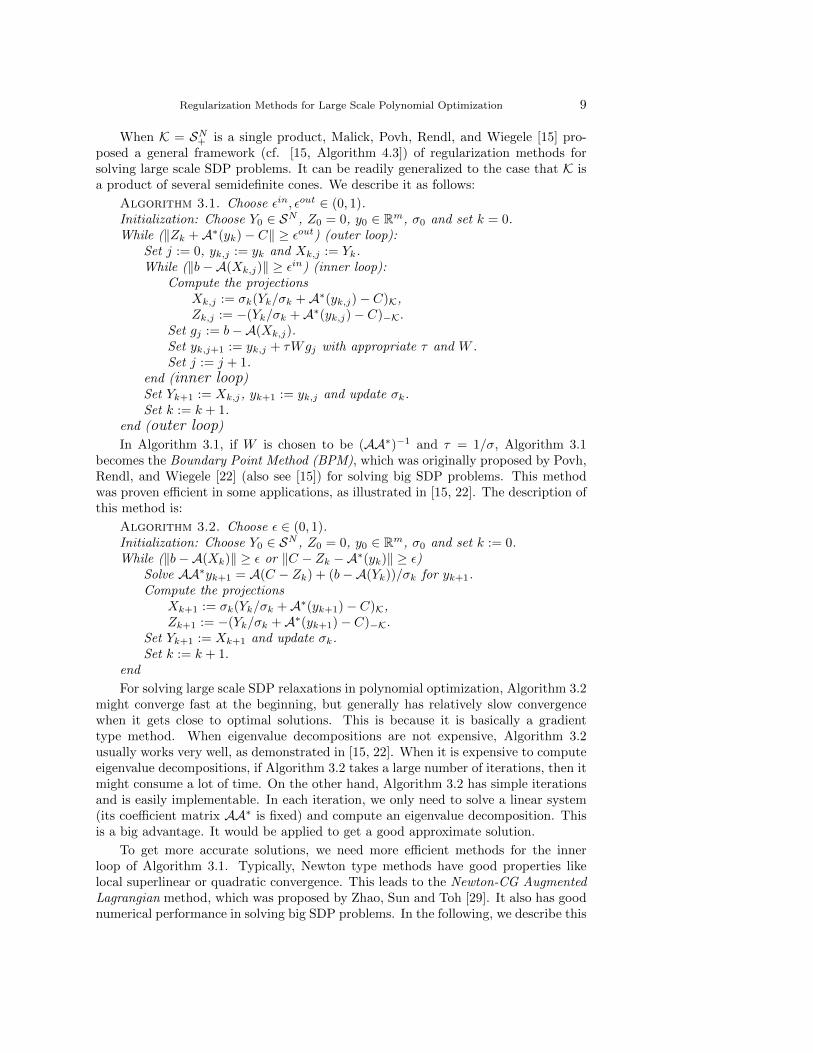
When K = SN+ is a single product, Malick, Povh, Rendl, and Wiegele [15] pro-
posed a general framework (cf. [15, Algorithm 4.3]) of regularization methods forsolving large scale SDP problems. It can be readily generalized to the case that K isa product of several semidefinite cones. We describe it as follows:
Algorithm 3.1. Choose εin, εout ∈ (0, 1).Initialization: Choose Y0 ∈ SN , Z0 = 0, y0 ∈ Rm, σ0 and set k = 0.While (‖Zk +A∗(yk)− C‖ ≥ εout) (outer loop):
Set j := 0, yk,j := yk and Xk,j := Yk.While (‖b−A(Xk,j)‖ ≥ εin) (inner loop):
Compute the projectionsXk,j := σk(Yk/σk +A∗(yk,j)− C)K,Zk,j := −(Yk/σk +A∗(yk,j)− C)−K.
Set gj := b−A(Xk,j).Set yk,j+1 := yk,j + τWgj with appropriate τ and W .Set j := j + 1.
end (inner loop)Set Yk+1 := Xk,j, yk+1 := yk,j and update σk.Set k := k + 1.
end (outer loop)In Algorithm 3.1, if W is chosen to be (AA∗)−1 and τ = 1/σ, Algorithm 3.1
becomes the Boundary Point Method (BPM), which was originally proposed by Povh,Rendl, and Wiegele [22] (also see [15]) for solving big SDP problems. This methodwas proven efficient in some applications, as illustrated in [15, 22]. The description ofthis method is:
Algorithm 3.2. Choose ε ∈ (0, 1).Initialization: Choose Y0 ∈ SN , Z0 = 0, y0 ∈ Rm, σ0 and set k := 0.While (‖b−A(Xk)‖ ≥ ε or ‖C − Zk −A∗(yk)‖ ≥ ε)
Solve AA∗yk+1 = A(C − Zk) + (b−A(Yk))/σk for yk+1.Compute the projections
Xk+1 := σk(Yk/σk +A∗(yk+1)− C)K,Zk+1 := −(Yk/σk +A∗(yk+1)− C)−K.
Set Yk+1 := Xk+1 and update σk.Set k := k + 1.
end
For solving large scale SDP relaxations in polynomial optimization, Algorithm 3.2might converge fast at the beginning, but generally has relatively slow convergencewhen it gets close to optimal solutions. This is because it is basically a gradienttype method. When eigenvalue decompositions are not expensive, Algorithm 3.2usually works very well, as demonstrated in [15, 22]. When it is expensive to computeeigenvalue decompositions, if Algorithm 3.2 takes a large number of iterations, then itmight consume a lot of time. On the other hand, Algorithm 3.2 has simple iterationsand is easily implementable. In each iteration, we only need to solve a linear system(its coefficient matrix AA∗ is fixed) and compute an eigenvalue decomposition. Thisis a big advantage. It would be applied to get a good approximate solution.
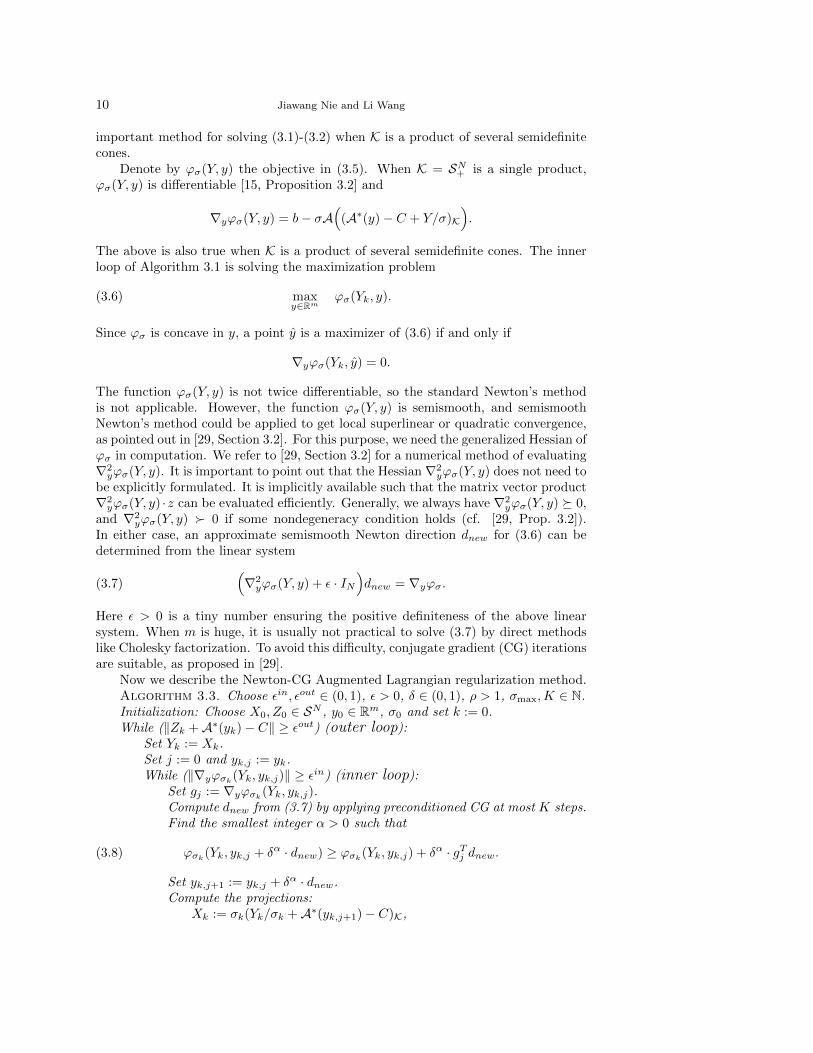
To get more accurate solutions, we need more efficient methods for the innerloop of Algorithm 3.1. Typically, Newton type methods have good properties likelocal superlinear or quadratic convergence. This leads to the Newton-CG AugmentedLagrangian method, which was proposed by Zhao, Sun and Toh [29]. It also has goodnumerical performance in solving big SDP problems. In the following, we describe this
10 Jiawang Nie and Li Wang
important method for solving (3.1)-(3.2) when K is a product of several semidefinitecones.
Denote by ϕσ(Y, y) the objective in (3.5). When K = SN+ is a single product,
ϕσ(Y, y) is differentiable [15, Proposition 3.2] and
∇yϕσ(Y, y) = b− σA((A∗(y)− C + Y/σ)K
).
The above is also true when K is a product of several semidefinite cones. The innerloop of Algorithm 3.1 is solving the maximization problem
(3.6) maxy∈Rm
ϕσ(Yk, y).
Since ϕσ is concave in y, a point y is a maximizer of (3.6) if and only if
∇yϕσ(Yk, y) = 0.
The function ϕσ(Y, y) is not twice differentiable, so the standard Newton’s methodis not applicable. However, the function ϕσ(Y, y) is semismooth, and semismoothNewton’s method could be applied to get local superlinear or quadratic convergence,as pointed out in [29, Section 3.2]. For this purpose, we need the generalized Hessian ofϕσ in computation. We refer to [29, Section 3.2] for a numerical method of evaluating∇2
yϕσ(Y, y). It is important to point out that the Hessian ∇2yϕσ(Y, y) does not need to
be explicitly formulated. It is implicitly available such that the matrix vector product∇2
yϕσ(Y, y) ·z can be evaluated efficiently. Generally, we always have ∇2yϕσ(Y, y) º 0,
and ∇2yϕσ(Y, y) Â 0 if some nondegeneracy condition holds (cf. [29, Prop. 3.2]).
In either case, an approximate semismooth Newton direction dnew for (3.6) can bedetermined from the linear system
(3.7)(∇2
yϕσ(Y, y) + ε · IN)dnew = ∇yϕσ.
Here ε > 0 is a tiny number ensuring the positive definiteness of the above linearsystem. When m is huge, it is usually not practical to solve (3.7) by direct methodslike Cholesky factorization. To avoid this difficulty, conjugate gradient (CG) iterationsare suitable, as proposed in [29].
Now we describe the Newton-CG Augmented Lagrangian regularization method.Algorithm 3.3. Choose εin, εout ∈ (0, 1), ε > 0, δ ∈ (0, 1), ρ > 1, σmax,K ∈ N.Initialization: Choose X0, Z0 ∈ SN , y0 ∈ Rm, σ0 and set k := 0.While (‖Zk +A∗(yk)− C‖ ≥ εout) (outer loop):
Set Yk := Xk.Set j := 0 and yk,j := yk.While (‖∇yϕσk
(Yk, yk,j)‖ ≥ εin) (inner loop):Set gj := ∇yϕσk
(Yk, yk,j).Compute dnew from (3.7) by applying preconditioned CG at most K steps.Find the smallest integer α > 0 such that
(3.8) ϕσk(Yk, yk,j + δα · dnew) ≥ ϕσk
(Yk, yk,j) + δα · gTj dnew.
Set yk,j+1 := yk,j + δα · dnew.Compute the projections:
Xk := σk(Yk/σk +A∗(yk,j+1)− C)K,
Regularization Methods for Large Scale Polynomial Optimization 11
Zk := −(Yk/σk +A∗(yk,j+1)− C)−K.Set j := j + 1.
end (inner loop)Set yk+1 := yk,j.If σk ≤ σmax, set σk+1 := ρσk.Set k := k + 1.
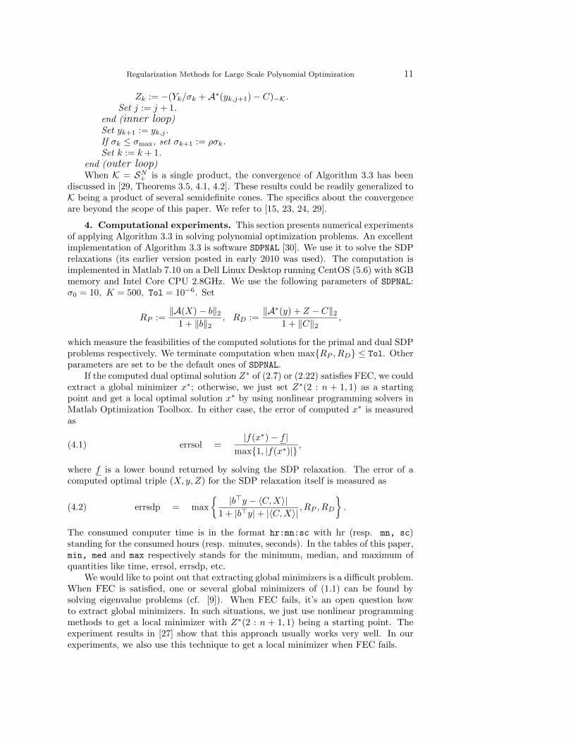
end (outer loop)When K = SN
+ is a single product, the convergence of Algorithm 3.3 has beendiscussed in [29, Theorems 3.5, 4.1, 4.2]. These results could be readily generalized toK being a product of several semidefinite cones. The specifics about the convergenceare beyond the scope of this paper. We refer to [15, 23, 24, 29].
4. Computational experiments. This section presents numerical experimentsof applying Algorithm 3.3 in solving polynomial optimization problems. An excellentimplementation of Algorithm 3.3 is software SDPNAL [30]. We use it to solve the SDPrelaxations (its earlier version posted in early 2010 was used). The computation isimplemented in Matlab 7.10 on a Dell Linux Desktop running CentOS (5.6) with 8GBmemory and Intel Core CPU 2.8GHz. We use the following parameters of SDPNAL:σ0 = 10, K = 500, Tol = 10−6. Set
RP :=‖A(X)− b‖21 + ‖b‖2 , RD :=
‖A∗(y) + Z − C‖21 + ‖C‖2 ,
which measure the feasibilities of the computed solutions for the primal and dual SDPproblems respectively. We terminate computation when max{RP , RD} ≤ Tol. Otherparameters are set to be the default ones of SDPNAL.
If the computed dual optimal solution Z∗ of (2.7) or (2.22) satisfies FEC, we couldextract a global minimizer x∗; otherwise, we just set Z∗(2 : n + 1, 1) as a startingpoint and get a local optimal solution x∗ by using nonlinear programming solvers inMatlab Optimization Toolbox. In either case, the error of computed x∗ is measuredas
(4.1) errsol =|f(x∗)− f |
max{1, |f(x∗)|} ,
where f is a lower bound returned by solving the SDP relaxation. The error of acomputed optimal triple (X, y, Z) for the SDP relaxation itself is measured as
(4.2) errsdp = max
{ |b>y − 〈C,X〉|1 + |b>y|+ |〈C,X〉| , RP , RD
}.
The consumed computer time is in the format hr:mn:sc with hr (resp. mn, sc)standing for the consumed hours (resp. minutes, seconds). In the tables of this paper,min, med and max respectively stands for the minimum, median, and maximum ofquantities like time, errsol, errsdp, etc.
We would like to point out that extracting global minimizers is a difficult problem.When FEC is satisfied, one or several global minimizers of (1.1) can be found bysolving eigenvalue problems (cf. [9]). When FEC fails, it’s an open question howto extract global minimizers. In such situations, we just use nonlinear programmingmethods to get a local minimizer with Z∗(2 : n + 1, 1) being a starting point. Theexperiment results in [27] show that this approach usually works very well. In ourexperiments, we also use this technique to get a local minimizer when FEC fails.
12 Jiawang Nie and Li Wang
The testing problems in our experiments are in three categories: (a) unconstrainedpolynomial optimization and it’s application in sensor network localization; (b) homo-geneous polynomial optimization and it’s application in computing stability numbers;(c) constrained polynomial optimization.
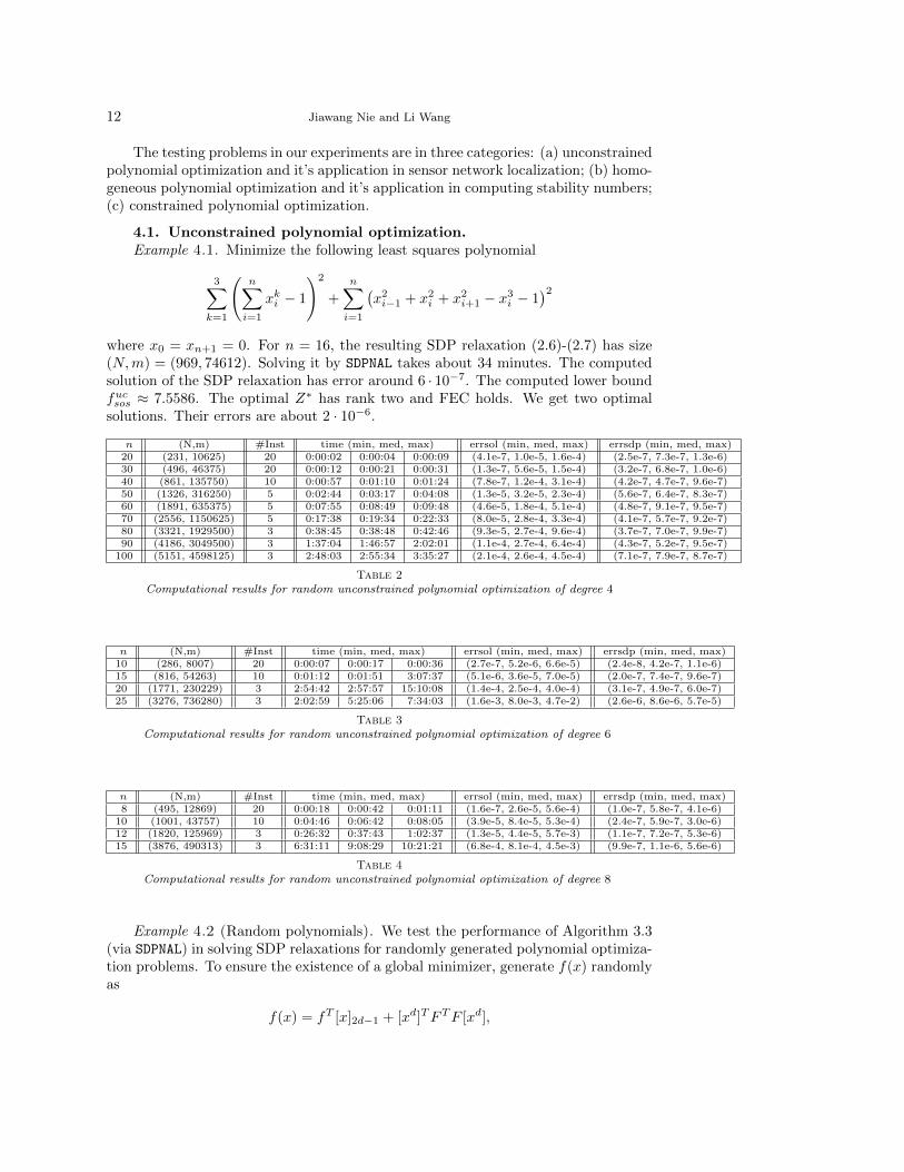
4.1. Unconstrained polynomial optimization.Example 4.1. Minimize the following least squares polynomial
3∑
k=1
(n∑
i=1
xki − 1
)2
+
n∑
i=1
(x2i−1 + x2
i + x2i+1 − x3
i − 1)2
where x0 = xn+1 = 0. For n = 16, the resulting SDP relaxation (2.6)-(2.7) has size(N,m) = (969, 74612). Solving it by SDPNAL takes about 34 minutes. The computedsolution of the SDP relaxation has error around 6 · 10−7. The computed lower boundfucsos ≈ 7.5586. The optimal Z∗ has rank two and FEC holds. We get two optimalsolutions. Their errors are about 2 · 10−6.
n (N,m) #Inst time (min, med, max) errsol (min, med, max) errsdp (min, med, max)20 (231, 10625) 20 0:00:02 0:00:04 0:00:09 (4.1e-7, 1.0e-5, 1.6e-4) (2.5e-7, 7.3e-7, 1.3e-6)30 (496, 46375) 20 0:00:12 0:00:21 0:00:31 (1.3e-7, 5.6e-5, 1.5e-4) (3.2e-7, 6.8e-7, 1.0e-6)40 (861, 135750) 10 0:00:57 0:01:10 0:01:24 (7.8e-7, 1.2e-4, 3.1e-4) (4.2e-7, 4.7e-7, 9.6e-7)50 (1326, 316250) 5 0:02:44 0:03:17 0:04:08 (1.3e-5, 3.2e-5, 2.3e-4) (5.6e-7, 6.4e-7, 8.3e-7)60 (1891, 635375) 5 0:07:55 0:08:49 0:09:48 (4.6e-5, 1.8e-4, 5.1e-4) (4.8e-7, 9.1e-7, 9.5e-7)70 (2556, 1150625) 5 0:17:38 0:19:34 0:22:33 (8.0e-5, 2.8e-4, 3.3e-4) (4.1e-7, 5.7e-7, 9.2e-7)80 (3321, 1929500) 3 0:38:45 0:38:48 0:42:46 (9.3e-5, 2.7e-4, 9.6e-4) (3.7e-7, 7.0e-7, 9.9e-7)90 (4186, 3049500) 3 1:37:04 1:46:57 2:02:01 (1.1e-4, 2.7e-4, 6.4e-4) (4.3e-7, 5.2e-7, 9.5e-7)
100 (5151, 4598125) 3 2:48:03 2:55:34 3:35:27 (2.1e-4, 2.6e-4, 4.5e-4) (7.1e-7, 7.9e-7, 8.7e-7)
Table 2Computational results for random unconstrained polynomial optimization of degree 4
n (N,m) #Inst time (min, med, max) errsol (min, med, max) errsdp (min, med, max)10 (286, 8007) 20 0:00:07 0:00:17 0:00:36 (2.7e-7, 5.2e-6, 6.6e-5) (2.4e-8, 4.2e-7, 1.1e-6)15 (816, 54263) 10 0:01:12 0:01:51 3:07:37 (5.1e-6, 3.6e-5, 7.0e-5) (2.0e-7, 7.4e-7, 9.6e-7)20 (1771, 230229) 3 2:54:42 2:57:57 15:10:08 (1.4e-4, 2.5e-4, 4.0e-4) (3.1e-7, 4.9e-7, 6.0e-7)25 (3276, 736280) 3 2:02:59 5:25:06 7:34:03 (1.6e-3, 8.0e-3, 4.7e-2) (2.6e-6, 8.6e-6, 5.7e-5)
Table 3Computational results for random unconstrained polynomial optimization of degree 6
n (N,m) #Inst time (min, med, max) errsol (min, med, max) errsdp (min, med, max)8 (495, 12869) 20 0:00:18 0:00:42 0:01:11 (1.6e-7, 2.6e-5, 5.6e-4) (1.0e-7, 5.8e-7, 4.1e-6)
10 (1001, 43757) 10 0:04:46 0:06:42 0:08:05 (3.9e-5, 8.4e-5, 5.3e-4) (2.4e-7, 5.9e-7, 3.0e-6)12 (1820, 125969) 3 0:26:32 0:37:43 1:02:37 (1.3e-5, 4.4e-5, 5.7e-3) (1.1e-7, 7.2e-7, 5.3e-6)15 (3876, 490313) 3 6:31:11 9:08:29 10:21:21 (6.8e-4, 8.1e-4, 4.5e-3) (9.9e-7, 1.1e-6, 5.6e-6)
Table 4Computational results for random unconstrained polynomial optimization of degree 8
Example 4.2 (Random polynomials). We test the performance of Algorithm 3.3(via SDPNAL) in solving SDP relaxations for randomly generated polynomial optimiza-tion problems. To ensure the existence of a global minimizer, generate f(x) randomlyas
f(x) = fT [x]2d−1 + [xd]TFTF [xd],

Regularization Methods for Large Scale Polynomial Optimization 13
n (N,m) #Inst time (min, med, max) errsol (min, med, max) errsdp (min, med, max)6 (462, 8007) 20 0:00:10 0:00:18 0:00:32 (3.6e-7, 1.4e-5, 1.4e-4) (3.2e-8, 5.2e-7, 3.1e-6)8 (1287, 43757) 10 0:04:13 0:05:33 0:10:23 (5.6e-6, 5.2e-5, 3.1e-4) (2.2e-7, 3.9e-7, 1.8e-6)9 (2002, 92377) 3 0:13:13 0:18:31 0:43:28 (2.2e-4, 7.3e-4, 8.4e-4) (1.1e-6, 2.5e-6, 2.9e-6)
10 (3003, 184755) 3 3:53:13 3:58:15 4:02:11 (2.3e-3, 2.4e-3, 4.1e-3) (4.7e-7, 1.2e-6, 4.2e-6)
Table 5Computational results for random unconstrained polynomial optimization of degree 10
where f/F is a Gaussian random vector/matrix of a proper dimension. Here [xd]denotes the vector of monomials of degree equal to d. The computational resultsare shown in Tables 2-5. There #Inst denotes the number of randomly generatedinstances, and (N,m) denotes the size of the corresponding SDP relaxation (2.6)-(2.7).
When f(x) has degree 4 (d = 2), SDP relaxation (2.6)-(2.7) is solved quite well.For n = 20 ∼ 30, the computation takes up to half a minute; for n = 40 ∼ 60, it takesa couple of minutes; for n = 70 ∼ 80, it takes less than one hour; for n = 90 ∼ 100,it takes a few hours. When f(x) has degree 6 (d = 3), for n = 15, solving (2.6)-(2.7)takes up to a few hours; for n = 20 ∼ 25, it takes a couple of hours. When f(x)has degree 8 (d = 4), for n = 10, solving (2.6)-(2.7) takes a couple of minutes; forn = 12 ∼ 15, it takes about one to ten hours. When f(x) has degree 10 (d = 5),for n = 8, solving (2.6)-(2.7) takes a couple of minutes; for n = 9, it takes less thanone hour; for n = 10, it takes a few hours. From Tables 2 to 5, we can see thatthe SDP relaxations are solved successfully. The obtained solutions for polynomialoptimization are also reasonably very well. They are slightly less accurate than thecomputed solutions of the SDP relaxation itself. This is probably because the SDPrelaxation (2.6)-(2.7) is not exact in minimizing the generated polynomials.
The computations here show that Algorithm 3.3 could solve large scale polynomialoptimization problems. A quartic polynomial optimization with 100 variables couldbe solved within a couple of hours on a regular computer. This is almost impossibleby using SDP solvers based on interior point methods.
Example 4.3 (Sensor Network Localization). Given a graph G = (V,E) and adistance for each edge, the sensor network localization problem is to find locations ofvertices so that their distances are equal to the desired ones. This problem can beformulated as follows: find a sequence of unknown vectors (sensors) u1, u2, . . . , us ∈Rk (typically k = 1, 2, 3, we focus on k = 2 in this example) such that the distancesbetween these sensors and some other fixed vectors (anchors) a1, . . . , a` are equal togiven distances. Recently, there is much work on solving sensor network localizationby SDP techniques, like [2, 13, 19]. Given edge subsets
ES ⊂ {(i, j) : 1 ≤ i < j ≤ s}, EA = {(i, j) : 1 ≤ i ≤ s, 1 ≤ j ≤ `},for every (i, j) ∈ ES , let dij be the distance between ui and uj , and for every (i, j) ∈ EA,let eij be the distance between ui and aj . Denote ui = (xki−k+1, . . . , xki) for i =1, . . . , s. The sensor network localization problem is equivalent to finding coordinatesxk1, . . . , xks satisfying the equations
‖ui − uj‖22 = d2ij ∀ (i, j) ∈ ES , ‖ui − aj‖22 = e2ij ∀ (i, j) ∈ EA.It is also equivalent to the quartic polynomial optimization problem
minu1,...,us
∑
(i,j)∈ES
(‖ui − uj‖22 − d2ij)2
+∑
(i,j)∈EA
(‖ui − aj‖22 − e2ij)2
.(4.3)

14 Jiawang Nie and Li Wang
Typically, it is large scale. We use SDPNAL to solve its SDP relaxation (2.6)-(2.7).To test its performance, we randomly generate sensors u1, . . . , us from the square
#sensor #Inst time (min, med, max) RMSD (min, med, max) errsdp (min, med, max)15 15 0:00:24 0:00:52 0:02:02 (8.1e-6, 2.4e-5, 1.4e-4) (1.1e-7, 4.2e-7, 1.6e-6)20 15 0:02:04 0:03:19 0:09:12 (1.5e-5, 5.5e-5, 1.5e-4) (2.9e-7, 4.4e-7, 2.0e-6)25 10 0:14:18 0:35:02 1:12:21 (4.3e-5, 8.7e-5, 2.2e-4) (2.4e-7, 6.3e-7, 1.6e-6)30 10 1:22:18 2:44:05 5:51:36 (2.3e-5, 2.3e-4, 2.7e-3) (9.2e-8, 1.8e-6, 5.3e-4)35 3 09:59:35 19:13:58 27:08:37 (1.3e-3, 1.6e-3, 2.2e-3) (6.5e-6, 5.1e-5, 6.5e-4)40 3 48:33:59 50:54:34 61:19:58 (1.2e-3, 1.6e-3, 2.7e-3) (2.2e-3, 3.2e-3, 4.0e-3)
Table 6Computational results for sensor network localization problems.
[−0.5, 0.5] × [−0.5, 0.5]. Fix four anchors as (±0.45, ±0.45). For each pair (i, j),select it to ES with probability 0.6 and to EA with probability 0.3. Then computeeach distance dij and eij . After the SDP relaxation is solved, we use Z∗(2 : n+ 1, 1)as a starting point and apply function lsqnonlin in Matlab Optimization Toolboxto get a local minimizer (u1, . . . , us) of (4.3) (we use the technique that was proposedin [13]). The errors of computed locations are measured by the Root Mean SquareDistance RMSD = ( 1sΣ
si=1‖ui − u∗
i ‖2)1/2, as used in [2].The computational results are shown in Table 6. We can see that the SDP
relaxation of (4.3) is solved reasonably well. In many instances, FEC is not satisfied,so we can only get a local minimizer of (4.3) by using the technique from [13]. Thetrue locations of sensors are found with small errors. Possible reasons for FEC failsmight be: the SDP relaxation was not solved accurately enough, or it is not exact for(4.3).
We would like to remark that the SDP relaxation (2.6)-(2.7) for (4.3) does notexploit the sparsity pattern. There exists work of using sparse SDP or SOS typerelaxations for solving sensor network localization problems (e.g., Kim et al. [13] andNie [19]). Generally, solving (2.6)-(2.7) for (4.3) is much more difficult than solvingits sparse versions like in [13, 19]. The numerical experiments in [13, 19] show thatexploiting sparsity will allow us to solve much bigger problems. However, in the viewof quality of approximations, sparse SDP relaxations are typically weaker than thegeneral dense one. Thus, it is still meaningful if we can solve (2.6)-(2.7) for large scalesensor network localization problems.
4.2. Homogeneous polynomial optimization.Example 4.4. Minimize the following square free quartic form over Sn−1
∑
1≤i<j<k<`≤n
(−i− j + k + `)xixjxkx`.
For n = 50, the resulting SDP (2.14)-(2.15) has size (N,m) = (1275, 292824). Solving(2.14)-(2.15) takes about 38 minutes. The error of the computed solution for the SDPrelaxation is around 8 · 10−8. The computed lower bound fhmg
sos ≈ −140.4051. Theoptimal Z∗ has rank two and FEC holds, so we get two optimizers. Their errors arearound 2 · 10−7.
Example 4.5. Minimize the following sextic form over Sn−1
∑
1≤i≤n
x6i +
∑
1≤i≤n−1
x3ix
3i+1.
For n = 20, the size of the resulting SDP (2.14)-(2.15) is (N,m) = (1540, 177099). Inthis problem, we set parameter Tol = 10−10 in running SDPNAL (For the default choice

Regularization Methods for Large Scale Polynomial Optimization 15
n (N,m) # Inst time (min, med, max) errsdp (min, med, max)20 (210, 8854) 20 0:00:06 0:00:11 0:00:26 (1.2e-7, 6.7e-7, 1.0e-6)30 (465, 40919) 20 0:00:45 0:01:21 0:01:52 (2.0e-7, 5.2e-7, 1.1e-6)40 (820, 123409) 10 0:02:31 0:05:19 0:08:58 (4.1e-7, 7.4e-7, 1.6e-6)50 (1275, 292824) 10 0:13:30 0:19:10 0:29:29 (4.5e-7, 5.9e-7, 9.6e-7)60 (1830, 595664) 5 0:44:19 1:05:32 1:47:51 (2.4e-7, 5.6e-7, 3.8e-6)70 (2485, 1088429) 5 2:33:24 4:20:13 5:07:37 (4.2e-7, 6.2e-7, 7.9e-7)80 (3240, 1837619) 3 7:31:21 9:43:40 10:52:27 (3.6e-7, 4.4e-7, 7.8e-7)90 (4095, 2919734) 3 17:10:41 17:44:02 18:45:28 (2.1e-7, 3.7e-7, 3.7e-7)
Table 7Computational results for stability number of random graphs
Tol = 10−6, SDPNAL does not converge very well for this example), i.e., we terminatethe computation when max{Rp, RD} < 10−10. Solving (2.14)-(2.15) takes about 2.5hours. The computed solution of the SDP relaxation has error around 1 · 10−5. Thecomputed lower bound fhmg
sos ≈ 1.1451 × 10⁻⁴. The computed optimal Z∗ has rankone and we get one global minimizer from it. Its error is around 1.3 · 10−5.
Example 4.6. Minimize the following sextic form over Sn−1
∑
1≤i<j<k≤n
x2ix
2jx
2k + x3
ix2jxk + x2
ix3jxk + xix
3jx
2k.
For n = 20, the resulting SDP (2.14)-(2.15) has size (N,m) = (1540, 177099). Solving(2.14)-(2.15) takes about 1.8 hours. The error of the computed solution of the SDPrelaxation is around 1.7 · 10−6. The computed lower bound fhmg
sos ≈ −0.3827. Thecomputed optimal Z∗ has rank one, so we get one global minimizer. Its error is around7.4 · 10−7.
An important application of homogenous polynomial optimization (2.8) is com-puting stability numbers of graphs.
Example 4.7 (Stability numbers of graphs). Let G = (V,E) be a graph with|V | = n. The stability number α(G) is the cardinality of the biggest stable subset(s)(their vertices are not connected by any edges) of V . It was shown in Motzkin andStraus [17] (also see De Klerk and Pasechnik [7]) that
α(G)−1 = minx∈∆n
xT (A+ In)x,
where ∆n is the standard simplex in Rn and A is the adjacency matrix associatedwith G. If replacing every xi ≥ 0 by x2
i , we get
(4.4) α(G)−1 = min‖x‖2=1
n∑
i=1
x4i + 2
∑
(i,j)∈E
x2ix
2j .
This is a quartic homogeneous polynomial optimization. When a lower bound fhmgsos of
(4.4) is computed from its SDP relaxation, we round(fhmgsos
)−1to the nearest integer
which will be used to estimate α(G).We generate random graphs G, and solve the SDP relaxation of (4.4). The gen-
eration of random graphs is in a similar way as in Bomze and De Klerk [3, Section 6].For n = 20, 30, 40, 50, 60, we generate random graphs G = (V,E) with |V | = n. Selecta random subset M ⊂ V with |M | = n/2. The edges eij({i, j} 6⊂ M) are generatedwith probability 1
2 . The computational results are in Table 7. As one can see, forn = 20, 30, 40, 50, solving (2.14)-(2.15) takes less than half an hour; for n = 60, 70,
16 Jiawang Nie and Li Wang
it takes a few hours; for n = 80, 90, it takes 7 to 19 hours. In all the instances,we get correct stability numbers. All the SDP relaxations themselves are also solvedsuccessively.
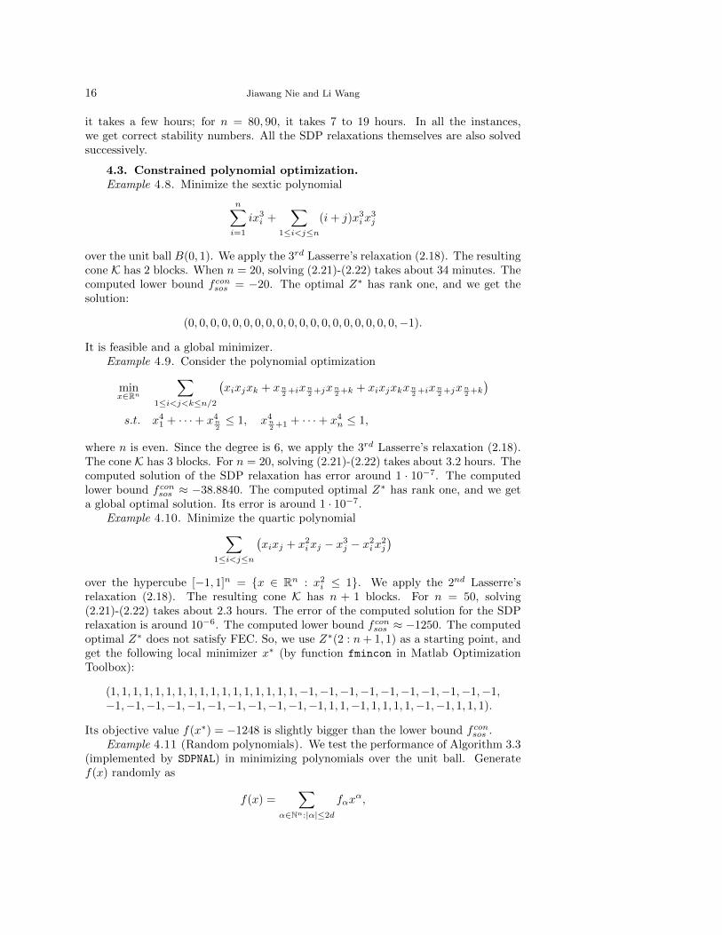
4.3. Constrained polynomial optimization.Example 4.8. Minimize the sextic polynomial
n∑
i=1
ix3i +
∑
1≤i<j≤n
(i+ j)x3ix
3j
over the unit ball B(0, 1). We apply the 3rd Lasserre’s relaxation (2.18). The resultingcone K has 2 blocks. When n = 20, solving (2.21)-(2.22) takes about 34 minutes. Thecomputed lower bound f con
sos = −20. The optimal Z∗ has rank one, and we get thesolution:
(0, 0, 0, 0, 0, 0, 0, 0, 0, 0, 0, 0, 0, 0, 0, 0, 0, 0, 0,−1).
It is feasible and a global minimizer.Example 4.9. Consider the polynomial optimization
minx∈Rn
∑
1≤i<j<k≤n/2
(xixjxk + xn
2 +ixn2 +jxn
2 +k + xixjxkxn2 +ixn
2 +jxn2 +k
)
s.t. x41 + · · ·+ x4
n2≤ 1, x4
n2 +1 + · · ·+ x4
n ≤ 1,
where n is even. Since the degree is 6, we apply the 3rd Lasserre’s relaxation (2.18).The cone K has 3 blocks. For n = 20, solving (2.21)-(2.22) takes about 3.2 hours. Thecomputed solution of the SDP relaxation has error around 1 · 10−7. The computedlower bound f con
sos ≈ −38.8840. The computed optimal Z∗ has rank one, and we geta global optimal solution. Its error is around 1 · 10−7.
Example 4.10. Minimize the quartic polynomial
∑
1≤i<j≤n
(xixj + x2
ixj − x3j − x2
ix2j
)
over the hypercube [−1, 1]n = {x ∈ Rn : x2i ≤ 1}. We apply the 2nd Lasserre’s
relaxation (2.18). The resulting cone K has n + 1 blocks. For n = 50, solving(2.21)-(2.22) takes about 2.3 hours. The error of the computed solution for the SDPrelaxation is around 10−6. The computed lower bound f con
sos ≈ −1250. The computedoptimal Z∗ does not satisfy FEC. So, we use Z∗(2 : n+ 1, 1) as a starting point, andget the following local minimizer x∗ (by function fmincon in Matlab OptimizationToolbox):
(1, 1, 1, 1, 1, 1, 1, 1, 1, 1, 1, 1, 1, 1, 1, 1, 1,−1,−1,−1,−1,−1,−1,−1,−1,−1,−1,−1,−1,−1,−1,−1,−1,−1,−1,−1,−1,−1, 1, 1,−1, 1, 1, 1, 1,−1,−1, 1, 1, 1).
Its objective value f(x∗) = −1248 is slightly bigger than the lower bound f consos .
Example 4.11 (Random polynomials). We test the performance of Algorithm 3.3(implemented by SDPNAL) in minimizing polynomials over the unit ball. Generatef(x) randomly as
f(x) =∑
α∈Nn:|α|≤2d
fαxα,

Regularization Methods for Large Scale Polynomial Optimization 17
(n,2d) #Inst time (min, med, max) errsol(min, med, max) errsdp(min, med, max)
(30,4) 10 0:00:28 0:00:52 0:02:47 (5.6e-8, 1.3e-6, 6.9e-6) (1.3e-7, 8.1e-7, 2.9e-6)
(40,4) 10 0:03:35 0:06:38 0:10:32 (8.8e-8, 1.8e-6, 9.5e-6) (2.2e-7, 1.0e-6, 4.5e-6)
(50,4) 3 0:20:34 0:22:18 0:24:59 (5.7e-6, 5.6e-6, 7.0e-6) (2.7e-6, 2.8e-6, 3.4e-6)
(60,4) 3 0:35:02 1:20:15 1:20:38 (1.5e-7, 3.5e-6, 2.5e-5) (1.7e-7, 1.7e-6, 1.2e-5)
(20,6) 3 0:36:31 0:49:17 0:56:35 (8.5e-7, 2.7e-6, 4.4e-6) (5.8e-7, 1.3e-6, 2.7e-6)
(12,8) 3 0:27:11 0:44:06 0:59:30 (5.5e-7, 2.8e-6, 9.0e-6) (9.0e-7, 1.3e-6, 4.2e-6)
(9,10) 3 0:16:31 0:36:05 0:40:53 (2.6e-7, 3.3e-6, 1.4e-5) (2.7e-7, 1.6e-6, 6.3e-6)
(80,4) 3 10:52:30 15:12:40 15:57:30 (5.3e-6, 5.5e-6, 2.2e-1) (2.6e-6, 2.6e-6, 2.7e-3)
(25,6) 3 10:38:04 11:00:48 12:57:59 (5.9e-3, 6.6e-3, 1.4e-2) (3.6e-3, 5.8e-3, 6.1e-3)
Table 8Computational results for random constrained polynomial optimization
where the coefficients fα are Gaussian random variables. We solve the SDP relaxation(2.21)-(2.22) by SDPNAL. The cases of degrees 4, 6, 8, 10 are tested. The computationalresults are in Table 8. When (n, 2d) = (80, 4) or (25, 6), the SDP relaxations are notsolved very well sometimes. This is probably because of the incurred ill-conditioning.In all the other cases, the SDP relaxations are solved quite well, and accurate globalminimizers are found.
5. Some discussions. In this section, we discuss some numerical issues aboutthe performance of regularization methods in solving SDP relaxations for large scalepolynomial optimization problems.
5.1. Scaling polynomial optimization. SDP relaxations arising from polyno-mial optimization are harder to solve than general SDP problems. A reason for this isthat the polynomials are not scaled very well sometimes. For instance, if the optimalZ∗ has rank 1, then Z∗ = [x∗]d[x∗]Td (x∗ is a minimizer) has entries of the form
1, x∗1, . . . , (x
∗1)
2, . . . , . . . , (x∗1)
2d, . . . , (x∗n)
2d.
Clearly, if some coordinate x∗i is small or big, then Z∗ is badly scaled and its entries
Z∗ij easily get underflow/overflow during the computation. This might cause severe ill-
conditioning in computations and make the computed solutions less accurate. Scalingis a useful approach to overcome this issue. In [10, 20], it was pointed out that scalingis important in solving polynomial optimization problems efficiently. Generally, thereis no simple rule to select the best scaling factor. In the following, we propose apractical scaling procedure.
Let s = (s1, . . . , sn) > 0 and scale x to x = (x1, . . . , xn) as
x = (s1x1, . . . , snxn).
Then f(x) is scaled to be the polynomial f(s1x1, . . . , snxn) in x. The best scalingfactor s should be such that the global minimizers of the scaled polynomial havecoordinates close to one or negative one. This is difficult because optimizers areusually unknown. However, as the algorithm runs, one often gets close to minimizersand would estimate them from the computations. Typically, we only need to scalethe problem when the algorithm fails to converge. Sometimes, we might need to doscaling several times. From our experiences, a practical scaling procedure is:Step 1 If Algorithm 3.3 converges well, we do no scaling and let it run; otherwise,
select a scaling vector s = (s1, . . . , sn) > 0 as:
(5.1) si =
{τ if |yei | ≤ τ,
|yei | otherwise.
Here τ > 0 is fixed and y is the most recent update for an optimal y∗ of (2.7).
18 Jiawang Nie and Li Wang
Step 2 Scale f(x) as f(s1x1, . . . , snxn). Go back to Step 1 and solve the scaledpolynomial optimization again.
In the above, τ > 0 is usually (but not too) small, because the coefficients of thescaled polynomial f(s1x1, . . . , snxn) should not be very tiny. We use τ = 10−3 in theexamples below.
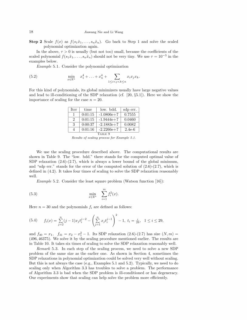
Example 5.1. Consider the polynomial optimization
(5.2) minx∈Rn
x41 + . . .+ x4
n +∑
1≤i<j<k≤n
xixjxk.
For this kind of polynomials, its global minimizers usually have large negative valuesand lead to ill-conditioning of the SDP relaxation (cf. [20, §5.1]). Here we show theimportance of scaling for the case n = 20.
Iter time low. bdd. sdp err.1 0:01:15 -1.0806e+7 0.75552 0:01:15 -1.9444e+7 0.04603 0:00:37 -2.1883e+7 0.00824 0:01:16 -2.2266e+7 2.4e-6
Table 9Results of scaling process for Example 5.1.
We use the scaling procedure described above. The computational results areshown in Table 9. The “low. bdd.” there stands for the computed optimal value ofSDP relaxation (2.6)-(2.7), which is always a lower bound of the global minimum,and “sdp err.” stands for the error of the computed solution of (2.6)-(2.7), which isdefined in (4.2). It takes four times of scaling to solve the SDP relaxation reasonablywell.
Example 5.2. Consider the least square problem (Watson function [16]):
(5.3) minx∈Rn
m∑
i=1
f2i (x).
Here n = 30 and the polynomials fi are defined as follows:
fi(x) =n∑
j=2
(j − 1)xjtj−2i −
(n∑
j=1
xjtj−1i
)2
− 1, ti =i29 , 1 ≤ i ≤ 29,(5.4)
and f30 = x1, f31 = x2 − x21 − 1. Its SDP relaxation (2.6)-(2.7) has size (N,m) =
(496, 46375). We solve it by the scaling procedure mentioned earlier. The results arein Table 10. It takes six times of scaling to solve the SDP relaxation reasonably well.
Remark 5.3. In each step of the scaling process, we need to solve a new SDPproblem of the same size as the earlier one. As shown in Section 4, sometimes theSDP relaxations in polynomial optimization could be solved very well without scaling.But this is not always the case (e.g., Examples 5.1 and 5.2). Typically, we need to doscaling only when Algorithm 3.3 has troubles to solve a problem. The performanceof Algorithm 3.3 is bad when the SDP problem is ill-conditioned or has degeneracy.Our experiments show that scaling can help solve the problem more efficiently.
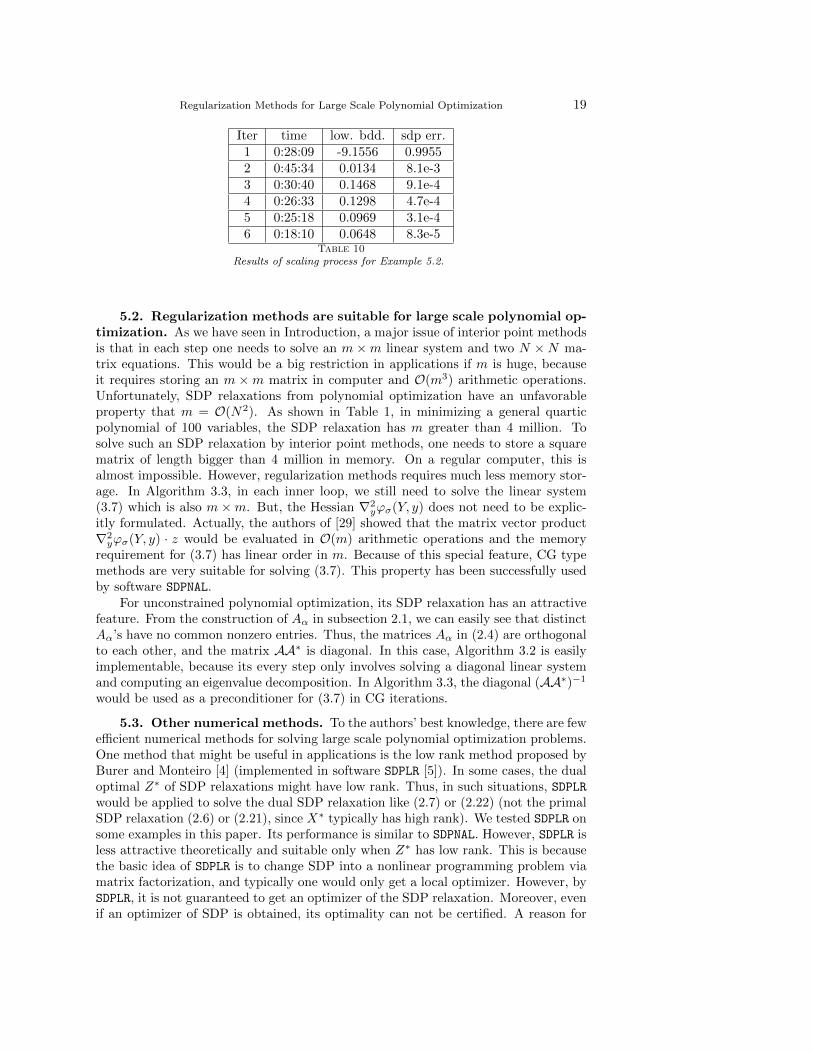
Regularization Methods for Large Scale Polynomial Optimization 19
Iter time low. bdd. sdp err.1 0:28:09 -9.1556 0.99552 0:45:34 0.0134 8.1e-33 0:30:40 0.1468 9.1e-44 0:26:33 0.1298 4.7e-45 0:25:18 0.0969 3.1e-46 0:18:10 0.0648 8.3e-5
Table 10Results of scaling process for Example 5.2.
5.2. Regularization methods are suitable for large scale polynomial op-timization. As we have seen in Introduction, a major issue of interior point methodsis that in each step one needs to solve an m ×m linear system and two N ×N ma-trix equations. This would be a big restriction in applications if m is huge, becauseit requires storing an m ×m matrix in computer and O(m3) arithmetic operations.Unfortunately, SDP relaxations from polynomial optimization have an unfavorableproperty that m = O(N2). As shown in Table 1, in minimizing a general quarticpolynomial of 100 variables, the SDP relaxation has m greater than 4 million. Tosolve such an SDP relaxation by interior point methods, one needs to store a squarematrix of length bigger than 4 million in memory. On a regular computer, this isalmost impossible. However, regularization methods requires much less memory stor-age. In Algorithm 3.3, in each inner loop, we still need to solve the linear system(3.7) which is also m ×m. But, the Hessian ∇2
yϕσ(Y, y) does not need to be explic-itly formulated. Actually, the authors of [29] showed that the matrix vector product∇2
yϕσ(Y, y) · z would be evaluated in O(m) arithmetic operations and the memoryrequirement for (3.7) has linear order in m. Because of this special feature, CG typemethods are very suitable for solving (3.7). This property has been successfully usedby software SDPNAL.
For unconstrained polynomial optimization, its SDP relaxation has an attractivefeature. From the construction of Aα in subsection 2.1, we can easily see that distinctAα’s have no common nonzero entries. Thus, the matrices Aα in (2.4) are orthogonalto each other, and the matrix AA∗ is diagonal. In this case, Algorithm 3.2 is easilyimplementable, because its every step only involves solving a diagonal linear systemand computing an eigenvalue decomposition. In Algorithm 3.3, the diagonal (AA∗)−1
would be used as a preconditioner for (3.7) in CG iterations.
5.3. Other numerical methods. To the authors’ best knowledge, there are fewefficient numerical methods for solving large scale polynomial optimization problems.One method that might be useful in applications is the low rank method proposed byBurer and Monteiro [4] (implemented in software SDPLR [5]). In some cases, the dualoptimal Z∗ of SDP relaxations might have low rank. Thus, in such situations, SDPLRwould be applied to solve the dual SDP relaxation like (2.7) or (2.22) (not the primalSDP relaxation (2.6) or (2.21), since X∗ typically has high rank). We tested SDPLR onsome examples in this paper. Its performance is similar to SDPNAL. However, SDPLR isless attractive theoretically and suitable only when Z∗ has low rank. This is becausethe basic idea of SDPLR is to change SDP into a nonlinear programming problem viamatrix factorization, and typically one would only get a local optimizer. However, bySDPLR, it is not guaranteed to get an optimizer of the SDP relaxation. Moreover, evenif an optimizer of SDP is obtained, its optimality can not be certified. A reason for
20 Jiawang Nie and Li Wang
this is that SDPLR is not a primal-dual type method, and typically a primal-dual pairis required to check optimality. On the other hand, the computational performanceof SDPLR is promising. It is an interesting future work to investigate properties of thelow rank method in solving polynomial optimization.
There are interesting recent work on solving large scale polynomial optimizationproblems by other methods. Bertsimas, Freund and Sun [1] proposed an acceleratedfirst order method to solve unconstrained polynomial optimization problems. A nicetheoretical property of first order type methods is that there are bounds on the com-plexity of computations, as proved in [1]. Henrion and Malick [11, 12] proposed aprojection method for solving conic optimization and SOS relaxations. These meth-ods can solve bigger problems than the interior point methods do, but they mighttake a big number of iterations to get an accurate optimal solution and generally itsconvergence is slow. In practical computations of solving big polynomial optimizationproblems, Algorithm 3.3 typically has faster convergence, because it uses second orderinformation (e.g., approximate Newton directions).
5.4. Convergence and nondegeneracy. The performance of Algorithm 3.3is not always very good for solving SDP relaxations in polynomial optimization. Aswe have seen earlier, a typical reason is the ill-conditioning. Another reason mightbe the degeneracy of the SDP relaxations. In [29], it was shown that if the SDPproblem is nondegenerate, then Algorithm 3.3 has good convergence; otherwise, itmight converge very badly or even does not converge. Generally, it is difficult tocheck in advance whether an SDP relaxation is degenerate or not. For SDP relaxation(2.6)-(2.7) in unconstrained polynomial optimization, or (2.21)-(2.22) in constrainedoptimization, a typical case for it to be degenerate is that a polynomial optimizationproblem has several distinct global minimizers. To see this for the unconstrainedpolynomial optimization (2.1), suppose it has two distinct global minimizers u∗, v∗
and the SOS relaxation (2.2) is exact. Then, the optimal values of (2.6) and (2.7)are equal, and (2.7) has two distinct optimal Z∗ (being [u∗]d[u∗]Td and [v∗]d[v∗]Td ).This implies the primal SDP relaxation (2.6) is degenerate. The situation is similarfor constrained polynomial optimization. From this observation, Algorithm 3.3 mightnot be very efficient if the SDP relaxation is exact and there are more than onedistinct optimizers. Of course, Algorithm 3.3 might still work if an SDP problem isdegenerate, like in Example 4.1. But this is occasional and typically not the case inpractice.
Acknowledgement The authors would like to thank Xinyuan Zhao, Defeng Sunand Kim-Chuan Toh for sharing their software SDPNAL, and Gabor Pataki for com-ments on the degeneracy of SDP. They also thank Bill Helton and Igor Klep for fruitfuldiscussions on this work.
REFERENCES
[1] D. Bertsimas, R. Freund, and X. Sun. An accelerated first-order method for solving uncon-strained SOS polynomial optimization problems. Optimization Methods and Software, toappear.
[2] P. Biswas and Y. Ye. Semidefinite programming for ad hoc wireless sensor network localization.Proc. 3rd IPSN, pp. 46–54, 2004.
[3] I.M. Bomze and E. de Klerk. Solving standard quadratic optimization problems via linear,semidefinite and copositive programming. Journal of Global Optimization, Vol. 24, No. 2,pp. 163–185, 2002.
[4] S. Burer and R. Monteiro. A nonlinear programming algorithm for solving semidefinite pro-
Regularization Methods for Large Scale Polynomial Optimization 21
grams via low-rank factorization. Mathematical Programming, Ser. B, Vol. 95, No. 2, pp.329–357, 2003.
[5] S. Burer. SDPLR: a C package for solving large-scale semidefinite programming problems.http://dollar.biz.uiowa.edu/~sburer
[6] R. Curto and L. Fialkow. Truncated K-moment problems in several variables. Journal of Op-erator Theory, 54, pp. 189–226, 2005.
[7] E. de Klerk and D.V. Pasechnik. Approximating of the stability number of a graph via copositiveprogramming. SIAM Journal on Optimization, Vol. 12, No. 4, pp. 875–892, 2002.
[8] K. Fujisawa, Y. Futakata, M. Kojima, S. Matsuyama, S. Nakamura, K. Nakata, andM. Yamashita. SDPA-M (SemiDefinite Programming Algorithm in MATLAB), http:
//homepage.mac.com/klabtitech/sdpa-homepage/download.html
[9] D. Henrion and J. Lasserre. Detecting global optimality and extracting solutions in GloptiPoly.Positive polynomials in control (Eds. D. Henrion, A. Garulli), Lecture Notes on Controland Information Sciences, Vol. 312, pp. 293–310, Springer, Berlin, 2005.
[10] D. Henrion and J. Lasserre. Gloptipoly: Global optimization over polynomials with matlab andsedumi. ACM Transactions on Mathematical Software, Vol. 29, No. 2, pp. 165–194, 2003.
[11] D. Henrion and J. Malick. Projection methods for conic feasibility problems: applications topolynomial sum-of-squares decompositions. Optimization Methods and Software, Vol. 26,No. 1, pp. 23–46, 2011.
[12] D. Henrion and J. Malick. Projection methods for conic optimization. LAAS-CNRS ResearchReport No.10730, 2010. Handbook of Semidefinite, Cone and Polynomial Optimization(Eds. M. Anjos and J. B. Lasserre), Springer, 2011.
[13] S. Kim, M. Kojima and H. Waki. Exploiting sparsity in SDP relaxation for sensor networklocalization. SIAM Journal on Optimization, Vol. 20, No. 1, pp. 192–215, 2009.
[14] J. Lasserre. Global optimization with polynomials and the problem of moments. SIAM Journalon Optimization, Vol. 11, No. 3, pp. 796–817, 2001.
[15] J. Malick, J. Povh, F. Rendl and A. Wiegele. Regularization methods for semidefinite program-ming. SIAM Journal on Optimization, Vol. 20, No. 1, pp. 336–356, 2009.
[16] J. More, B. Garbow and K. Hillstrom. Testing unconstrained optimization software. ACMTrans. Math. Soft., Vol. 7, pp. 17–41, 1981.
[17] T.S. Motzkin and E.G. Straus. Maxima for graphs and a new proof of a theorem of Turan.Canadian J. Math., 17, pp. 533–540, 1965.
[18] J. Nie and J. Demmel. Sparse SOS relaxations for minimizing functions that are summations ofsmall polynomials. SIAM Journal On Optimization, Vol. 19, No. 4, pp. 1534–1558, 2008.
[19] J. Nie. Sum of squares method for sensor network localization. Computational Optimizationand Applications, Vol. 43, No. 2, pp. 151–179, 2009.
[20] P. Parrilo and B. Sturmfels. Minimizing polynomial functions. Proceedings of the DIMACSWorkshop on Algorithmic and Quantitative Aspects of Real Algebraic Geometry in Mathe-matics and Computer Science (March 2001) (eds. S. Basu and L. Gonzalez-Vega), pp. 83–100, American Mathematical Society, 2003.
[21] P. Parrilo. Semidefinite programming relaxations for semialgebraic problems. Math. Program.,Ser. B, Vol. 96, No. 2, pp. 293–320, 2003.
[22] J. Povh, F. Rendl, and A. Wiegele. A boundary point method to solve semidefinite programs.Computing, Vol. 78, pp. 277–286, 2006.
[23] R.T. Rockafellar. Monotone operators and the proximal point algorithm. SIAM J. Control andOptim., Vol. 14, No. 5, pp. 877–898, 1976.
[24] R.T. Rockafellar. Augmented Lagrangians and applications of the proximal point algorithm inconvex programming. Math. Oper. Res. , Vol. 1, No. 2, pp. 97–116, 1976.
[25] J.F. Sturm. SeDuMi 1.02:a MATLAB toolbox for optimization over symmetric cones. Opti-mization Methods and Software, 11 & 12, No. 1-4, pp. 625–653, 1999.
[26] K.C. Toh, M.J. Todd, and R.H. Tutuncu. SDPT3: a Matlab software package for semidefiniteprogramming. Optimization Methods and Software, Vol. 11, pp. 545–581, 1999.
[27] H. Waki, S. Kim, M. Kojima and M. Muramatsu. Sums of squares and semidefinite program-ming relaxations for polynomial optimization problems with Structured Sparsity. SIAMJournal on Optimization, Vol.17, No. 1, pp. 218–242, 2006.
[28] H. Wolkowicz, R. Saigal, and L. Vandenberghe, editors. Handbook of semidefinite programming,Kluwer, Publisher, 2000.
[29] X.Y. Zhao, D.F. Sun, and K.C. Toh. A Newton-CG Augmented Lagrangian method for semidef-inite programming. SIAM Journal on Optimization, Vol. 20, No. 4, pp. 1737–1765, 2010.
[30] X.Y. Zhao, D.F. Sun, and K.C. Toh. SDPNAL version 0.1 – a MATLAB software for semidef-inite programming based on a semi-smooth Newton-CG augmented Lagrangian method.http://www.math.nus.edu.sg/~mattohkc/SDPNAL.html