regressione: processi gaussiani e machine...
TRANSCRIPT
Corso di Sistemi di Elaborazione dell’Informazione
Prof. Giuseppe Boccignone
Dipartimento di Informatica
Università di Milano
boccignone.di.unimi.it/FM_2016.html
SCUOLA DI SPECIALIZZAZIONE IN FISICA MEDICA
Regressione: processi Gaussiani e Machine Learning
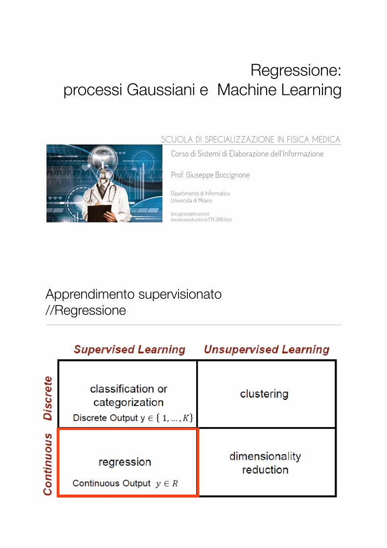
Apprendimento supervisionato //Regressione
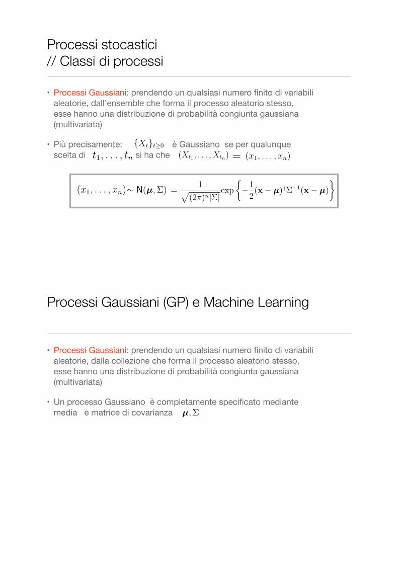
• Processi Gaussiani: prendendo un qualsiasi numero finito di variabili aleatorie, dall’ensemble che forma il processo aleatorio stesso, esse hanno una distribuzione di probabilità congiunta gaussiana (multivariata)
• Più precisamente: è Gaussiano se per qualunque scelta di si ha che
Processi stocastici // Classi di processi
Chapter 3
Gaussian Processes andStochastic DifferentialEquations
3.1 Gaussian Processes
Gaussian processes are a reasonably large class of processes that havemany applications, including in finance, time-series analysis and machinelearning. Certain classes of Gaussian processes can also be thought of asspatial processes. We will use these as a vehicle to start considering moregeneral spatial objects.
Definition 3.1.1 (Gaussian Process). A stochastic process {Xt}t≥0 is Gaus-sian if, for any choice of times t1, . . . , tn, the random vector (Xt1 , . . . , Xtn)has a multivariate normal distribution.
3.1.1 The Multivariate Normal Distribution
Because Gaussian processes are defined in terms of the multivariate nor-mal distribution, we will need to have a pretty good understanding of thisdistribution and its properties.
Definition 3.1.2 (Multivariate Normal Distribution). A vectorX = (X1, . . . , Xn)is said to be multivariate normal (multivariate Gaussian) if all linear combi-nations of X, i.e. all random variables of the form
n!
k=1
αkXk
have univariate normal distributions.
89
3.1. GAUSSIAN PROCESSES 93
Simulating Multivariate Normals
One possible way to simulate a multivariate normal random vector isusing the Cholesky decomposition.
Lemma 3.1.11. If Z ∼ N(0, I), Σ = AA! is a covariance matrix, andX = µ+ AZ, then X ∼ N(µ,Σ).
Proof. We know from lemma 3.1.4 that AZ is multivariate normal and sois µ + AZ. Because a multivariate normal random vector is completelydescribed by its mean vector and covariance matrix, we simple need to findEX and Var(X). Now,
EX = Eµ+ EAZ = µ+ A0 = µ
and
Var(X) = Var(µ+ AZ) = Var(AZ) = AVar(Z)A! = AIA! = AA! = Σ.
Thus, we can simulate a random vector X ∼ N(µ,Σ) by
(i) Finding A such that Σ = AA!.
(ii) Generating Z ∼ N(0, I).
(iii) Returning X = µ+ AZ.
Matlab makes things a bit confusing because its function ‘chol’ producesa decomposition of the form B!B. That is, A = B!. It is important tobe careful and think about whether you want to generate a row or columnvector when generating multivariate normals.
The following code produces column vectors.
Listing 3.1: Matlab code
1 mu = [1 2 3]’;
2 Sigma = [3 1 2; 1 2 1; 2 1 5];
3 A = chol(Sigma);
4 X = mu + A’ * randn(3,1);
The following code produces row vectors.
Listing 3.2: Matlab code
1 mu = [1 2 3];
2 Sigma = [3 1 2; 1 2 1; 2 1 5];
3 A = chol(Sigma);
4 X = mu + randn(1,3) * A;
92 CHAPTER 3. GAUSSIAN PROCESSES ETC.
If A is also symmetric, then A is called symmetric positive semi-definite(SPSD). Note that if A is an SPSD then there is a real-valued decomposition
A = LL!,
though it is not necessarily unique and L may have zeroes on the diagonals.
Lemma 3.1.9. Covariance matrices are SPSD.
Proof. Given an n × 1 real-valued vector x and a random vector Y withcovariance matrix Σ, we have
Var (x!Y) = x!Var (Y)x.
Now this must be non-negative (as it is a variance). That is, it must be thecase that
x!Var (Y)x ≥ 0,
so Σ is positive semi-definite. Symmetry comes from the fact that Cov(X, Y ) =Cov(Y,X).
Lemma 3.1.10. SPSD matrices are covariance matrices.
Proof. Let A be an SPSD matrix and Z be a vector of random variables withVar(Z) = I. Now, as A is SPSD, A = LL!. So,
Var(LZ) = LVar(Z)L! = LIL! = A,
so A is the covariance matrix of LZ.
COVARIANCE POS DEF ...
Densities of Multivariate Normals
If X = (X1, . . . , Xn) is N(µ,Σ) and Σ is positive definite, then X has thedensity
f(x) = f(x1, . . . , xn) =1!
(2π)n|Σ|exp
"−1
2(x− µ)!Σ−1(x− µ)
#.
Chapter 3
Gaussian Processes andStochastic DifferentialEquations
3.1 Gaussian Processes
Gaussian processes are a reasonably large class of processes that havemany applications, including in finance, time-series analysis and machinelearning. Certain classes of Gaussian processes can also be thought of asspatial processes. We will use these as a vehicle to start considering moregeneral spatial objects.
Definition 3.1.1 (Gaussian Process). A stochastic process {Xt}t≥0 is Gaus-sian if, for any choice of times t1, . . . , tn, the random vector (Xt1 , . . . , Xtn)has a multivariate normal distribution.
3.1.1 The Multivariate Normal Distribution
Because Gaussian processes are defined in terms of the multivariate nor-mal distribution, we will need to have a pretty good understanding of thisdistribution and its properties.
Definition 3.1.2 (Multivariate Normal Distribution). A vectorX = (X1, . . . , Xn)is said to be multivariate normal (multivariate Gaussian) if all linear combi-nations of X, i.e. all random variables of the form
n!
k=1
αkXk
have univariate normal distributions.
89
92 CHAPTER 3. GAUSSIAN PROCESSES ETC.
If A is also symmetric, then A is called symmetric positive semi-definite(SPSD). Note that if A is an SPSD then there is a real-valued decomposition
A = LL!,
though it is not necessarily unique and L may have zeroes on the diagonals.
Lemma 3.1.9. Covariance matrices are SPSD.
Proof. Given an n × 1 real-valued vector x and a random vector Y withcovariance matrix Σ, we have
Var (x!Y) = x!Var (Y)x.
Now this must be non-negative (as it is a variance). That is, it must be thecase that
x!Var (Y)x ≥ 0,
so Σ is positive semi-definite. Symmetry comes from the fact that Cov(X, Y ) =Cov(Y,X).
Lemma 3.1.10. SPSD matrices are covariance matrices.
Proof. Let A be an SPSD matrix and Z be a vector of random variables withVar(Z) = I. Now, as A is SPSD, A = LL!. So,
Var(LZ) = LVar(Z)L! = LIL! = A,
so A is the covariance matrix of LZ.
COVARIANCE POS DEF ...
Densities of Multivariate Normals
If X = (X1, . . . , Xn) is N(µ,Σ) and Σ is positive definite, then X has thedensity
f(x) = f(x1, . . . , xn) =1!
(2π)n|Σ|exp
"−1
2(x− µ)!Σ−1(x− µ)
#.
Processi Gaussiani (GP) e Machine Learning
• Processi Gaussiani: prendendo un qualsiasi numero finito di variabili aleatorie, dalla collezione che forma il processo aleatorio stesso, esse hanno una distribuzione di probabilità congiunta gaussiana (multivariata)
• Un processo Gaussiano è completamente specificato mediante media e matrice di covarianza
3.1. GAUSSIAN PROCESSES 93
Simulating Multivariate Normals
One possible way to simulate a multivariate normal random vector isusing the Cholesky decomposition.
Lemma 3.1.11. If Z ∼ N(0, I), Σ = AA! is a covariance matrix, andX = µ+ AZ, then X ∼ N(µ,Σ).
Proof. We know from lemma 3.1.4 that AZ is multivariate normal and sois µ + AZ. Because a multivariate normal random vector is completelydescribed by its mean vector and covariance matrix, we simple need to findEX and Var(X). Now,
EX = Eµ+ EAZ = µ+ A0 = µ
and
Var(X) = Var(µ+ AZ) = Var(AZ) = AVar(Z)A! = AIA! = AA! = Σ.
Thus, we can simulate a random vector X ∼ N(µ,Σ) by
(i) Finding A such that Σ = AA!.
(ii) Generating Z ∼ N(0, I).
(iii) Returning X = µ+ AZ.
Matlab makes things a bit confusing because its function ‘chol’ producesa decomposition of the form B!B. That is, A = B!. It is important tobe careful and think about whether you want to generate a row or columnvector when generating multivariate normals.
The following code produces column vectors.
Listing 3.1: Matlab code
1 mu = [1 2 3]’;
2 Sigma = [3 1 2; 1 2 1; 2 1 5];
3 A = chol(Sigma);
4 X = mu + A’ * randn(3,1);
The following code produces row vectors.
Listing 3.2: Matlab code
1 mu = [1 2 3];
2 Sigma = [3 1 2; 1 2 1; 2 1 5];
3 A = chol(Sigma);
4 X = mu + randn(1,3) * A;
Processi stocastici // Simulazione di processi Gaussiani
94 CHAPTER 3. GAUSSIAN PROCESSES ETC.
The complexity of the Cholesky decomposition of an arbitrary real-valuedmatrix is O(n3) floating point operations.
3.1.2 Simulating a Gaussian Processes Version 1
Because Gaussian processes are defined to be processes where, for anychoice of times t1, . . . , tn, the random vector (Xt1 , . . . , Xtn) has a multivariatenormal density and a multivariate normal density is completely describe bya mean vector µ and a covariance matrix Σ, the probability distribution ofGaussian process is completely described if we have a way to construct themean vector and covariance matrix for an arbitrary choice of t1, . . . , tn.
We can do this using an expectation function
µ(t) = EXt
and a covariance function
r(s, t) = Cov(Xs, Xt).
Using these, we can simulate the values of a Gaussian process at fixed timest1, . . . , tn by calculating µ where µi = µ(t1) and Σ, where Σi,j = r(ti, tj) andthen simulating a multivariate normal vector.
In the following examples, we simulate the Gaussian processes at evenlyspaced times t1 = 1/h, t2 = 2/h, . . . , tn = 1.
Example 3.1.12 (Brownian Motion). Brownian motion is a very importantstochastic process which is, in some sense, the continuous time continuousstate space analogue of a simple random walk. It has an expectation functionµ(t) = 0 and a covariance function r(s, t) = min(s, t).
Listing 3.3: Matlab code
1 %use mesh size h
2 m = 1000; h = 1/m; t = h : h : 1;
3 n = length(t);
4
5 %Make the mean vector
6 mu = zeros(1,n);
7 for i = 1:n
8 mu(i) = 0;
9 end
10
11 %Make the covariance matrix
12 Sigma = zeros(n,n);
3.1. GAUSSIAN PROCESSES 95
13 for i = 1:n
14 for j = 1:n
15 Sigma(i,j) = min(t(i),t(j));
16 end
17 end
18
19 %Generate the multivariate normal vector
20 A = chol(Sigma);
21 X = mu + randn(1,n) * A;
22
23 %Plot
24 plot(t,X);
0 0.1 0.2 0.3 0.4 0.5 0.6 0.7 0.8 0.9 1−1.8
−1.6
−1.4
−1.2
−1
−0.8
−0.6
−0.4
−0.2
0
0.2
t
Xt
Figure 3.1.1: Plot of Brownain motion on [0, 1].
Example 3.1.13 (Ornstein-Uhlenbeck Process). Another very importantGaussian process is the Ornstein-Uhlenbeck process. This has expectationfunction µ(t) = 0 and covariance function r(s, t) = e−α|s−t|/2.
Listing 3.4: Matlab code
1 %use mesh size h
2 m = 1000; h = 1/m; t = h : h : 1;
3 n = length(t);
4 %paramter of OU process
5 alpha = 10;
6
96 CHAPTER 3. GAUSSIAN PROCESSES ETC.
7 %Make the mean vector
8 mu = zeros(1,n);
9 for i = 1:n
10 mu(i) = 0;
11 end
12
13 %Make the covariance matrix
14 Sigma = zeros(n,n);
15 for i = 1:n
16 for j = 1:n
17 Sigma(i,j) = exp(-alpha * abs(t(i) - t(j)) / 2);
18 end
19 end
20
21 %Generate the multivariate normal vector
22 A = chol(Sigma);
23 X = mu + randn(1,n) * A;
24
25 %Plot
26 plot(t,X);
0 0.1 0.2 0.3 0.4 0.5 0.6 0.7 0.8 0.9 1−1.5
−1
−0.5
0
0.5
1
1.5
2
2.5
3
t
Xt
Figure 3.1.2: Plot of an Ornstein-Uhlenbeck process on [0, 1] with α = 10.
Example 3.1.14 (Fractional Brownian Motion). Fractional Brownian mo-tion (fBm) is a generalisation of Brownian Motion. It has expectation func-tion µ(t) = 0 and covariance function Cov(s, t) = 1/2(t2H + s2H − |t− s|2H),
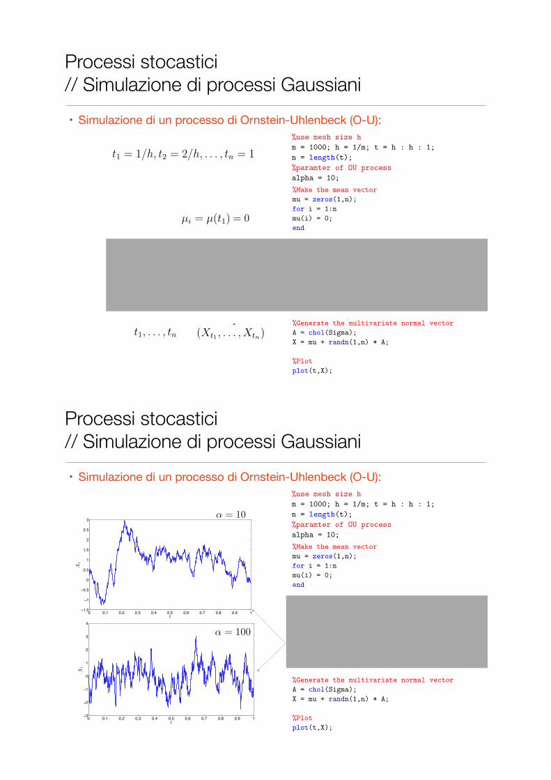
• Simulazione di un processo di Ornstein-Uhlenbeck (O-U):
Processi stocastici // Simulazione di processi Gaussiani • Simulazione di un processo di Ornstein-Uhlenbeck (O-U):
3.1. GAUSSIAN PROCESSES 95
13 for i = 1:n
14 for j = 1:n
15 Sigma(i,j) = min(t(i),t(j));
16 end
17 end
18
19 %Generate the multivariate normal vector
20 A = chol(Sigma);
21 X = mu + randn(1,n) * A;
22
23 %Plot
24 plot(t,X);
0 0.1 0.2 0.3 0.4 0.5 0.6 0.7 0.8 0.9 1−1.8
−1.6
−1.4
−1.2
−1
−0.8
−0.6
−0.4
−0.2
0
0.2
t
Xt
Figure 3.1.1: Plot of Brownain motion on [0, 1].
Example 3.1.13 (Ornstein-Uhlenbeck Process). Another very importantGaussian process is the Ornstein-Uhlenbeck process. This has expectationfunction µ(t) = 0 and covariance function r(s, t) = e−α|s−t|/2.
Listing 3.4: Matlab code
1 %use mesh size h
2 m = 1000; h = 1/m; t = h : h : 1;
3 n = length(t);
4 %paramter of OU process
5 alpha = 10;
6
96 CHAPTER 3. GAUSSIAN PROCESSES ETC.
7 %Make the mean vector
8 mu = zeros(1,n);
9 for i = 1:n
10 mu(i) = 0;
11 end
12
13 %Make the covariance matrix
14 Sigma = zeros(n,n);
15 for i = 1:n
16 for j = 1:n
17 Sigma(i,j) = exp(-alpha * abs(t(i) - t(j)) / 2);
18 end
19 end
20
21 %Generate the multivariate normal vector
22 A = chol(Sigma);
23 X = mu + randn(1,n) * A;
24
25 %Plot
26 plot(t,X);
0 0.1 0.2 0.3 0.4 0.5 0.6 0.7 0.8 0.9 1−1.5
−1
−0.5
0
0.5
1
1.5
2
2.5
3
t
Xt
Figure 3.1.2: Plot of an Ornstein-Uhlenbeck process on [0, 1] with α = 10.
Example 3.1.14 (Fractional Brownian Motion). Fractional Brownian mo-tion (fBm) is a generalisation of Brownian Motion. It has expectation func-tion µ(t) = 0 and covariance function Cov(s, t) = 1/2(t2H + s2H − |t− s|2H),
3.1. GAUSSIAN PROCESSES 97
0 0.1 0.2 0.3 0.4 0.5 0.6 0.7 0.8 0.9 1−3
−2
−1
0
1
2
3
4
t
Xt
Figure 3.1.3: Plot of an Ornstein-Uhlenbeck process on [0, 1] with α = 100.
where H ∈ (0, 1) is called the Hurst parameter. When H = 1/2, fBm re-duces to standard Brownian motion. Brownian motion has independent in-crements. In contrast, for H > 1/2 fBm has positively correlated incrementsand for H < 1/2 fBm has negatively correlated increments.
Listing 3.5: Matlab code
1 %Hurst parameter
2 H = .9;
3
4 %use mesh size h
5 m = 1000; h = 1/m; t = h : h : 1;
6 n = length(t);
7
8 %Make the mean vector
9 mu = zeros(1,n);
10 for i = 1:n
11 mu(i) = 0;
12 end
13
14 %Make the covariance matrix
15 Sigma = zeros(n,n);
16 for i = 1:n
17 for j = 1:n
18 Sigma(i,j) = 1/2 * (t(i)^(2*H) + t(j)^(2*H)...
19 - (abs(t(i) - t(j)))^(2 * H));
96 CHAPTER 3. GAUSSIAN PROCESSES ETC.
7 %Make the mean vector
8 mu = zeros(1,n);
9 for i = 1:n
10 mu(i) = 0;
11 end
12
13 %Make the covariance matrix
14 Sigma = zeros(n,n);
15 for i = 1:n
16 for j = 1:n
17 Sigma(i,j) = exp(-alpha * abs(t(i) - t(j)) / 2);
18 end
19 end
20
21 %Generate the multivariate normal vector
22 A = chol(Sigma);
23 X = mu + randn(1,n) * A;
24
25 %Plot
26 plot(t,X);
0 0.1 0.2 0.3 0.4 0.5 0.6 0.7 0.8 0.9 1−1.5
−1
−0.5
0
0.5
1
1.5
2
2.5
3
t
Xt
Figure 3.1.2: Plot of an Ornstein-Uhlenbeck process on [0, 1] with α = 10.
Example 3.1.14 (Fractional Brownian Motion). Fractional Brownian mo-tion (fBm) is a generalisation of Brownian Motion. It has expectation func-tion µ(t) = 0 and covariance function Cov(s, t) = 1/2(t2H + s2H − |t− s|2H),
Processi Gaussiani (GP) e Machine Learning
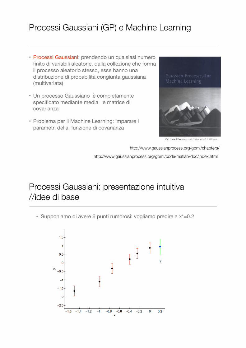
• Processi Gaussiani: prendendo un qualsiasi numero finito di variabili aleatorie, dalla collezione che forma il processo aleatorio stesso, esse hanno una distribuzione di probabilità congiunta gaussiana (multivariata)
• Un processo Gaussiano è completamente specificato mediante media e matrice di covarianza
• Problema per il Machine Learning: imparare i parametri della funzione di covarianza
Further reading
Many more topics and code:http://www.gaussianprocess.org/gpml/
MCMC inference for GPs is implemented in FBM:http://www.cs.toronto.edu/~radford/fbm.software.html
Gaussian processes for ordinal regression, Chu and Ghahramani,JMLR, 6:1019–1041, 2005.
Flexible and e�cient Gaussian process models for machine learning,Edward L. Snelson, PhD thesis, UCL, 2007.
http://www.gaussianprocess.org/gpml/chapters/
http://www.gaussianprocess.org/gpml/code/matlab/doc/index.html
Processi Gaussiani: presentazione intuitiva //idee di base
• Supponiamo di avere 6 punti rumorosi: vogliamo predire a x*=0.2

Processi Gaussiani //idee di base
• Supponiamo di avere 6 punti rumorosi: vogliamo predire a x*=0.2
• Non assumiamo un modello parametrico, esempio:
• Lasciamo che i dati parlino da soli
• Assumiamo che i dati siano stati generati da una distribuzione Gaussiana n-variata
Processi Gaussiani //idee di base
• Assumiamo che i dati siano stati generati da una distribuzione Gaussiana n-variata:
• media 0
• funzione di covarianza k(x,x’)
• Caratteristiche di k(x,x’)
• massima per x vicino a x’
• se x lontano da x’
• esempio:
x vicino a x’
y correlato a y’
Processi Gaussiani //idee di base
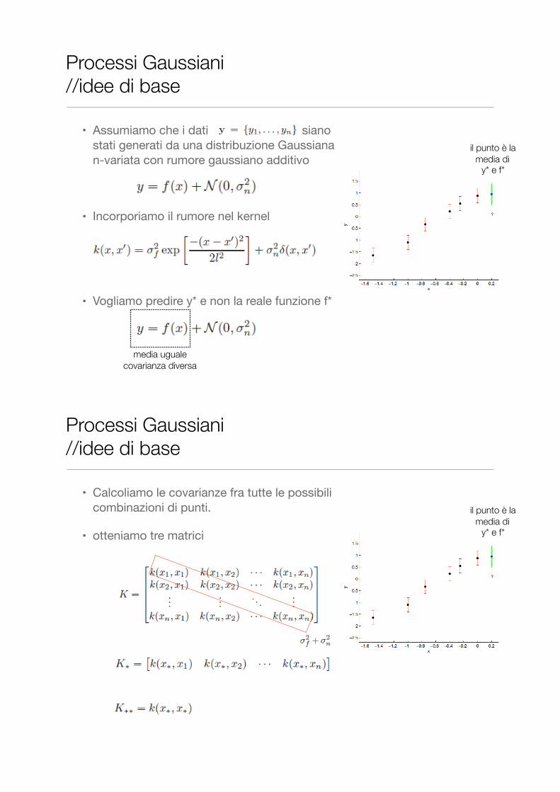
• Assumiamo che i dati siano stati generati da una distribuzione Gaussiana n-variata con rumore gaussiano additivo
• Incorporiamo il rumore nel kernel
• Vogliamo predire y* e non la reale funzione f*
il punto è la media di
y* e f*
media uguale covarianza diversa
Processi Gaussiani //idee di base
• Calcoliamo le covarianze fra tutte le possibili combinazioni di punti.
• otteniamo tre matrici
il punto è la media di
y* e f*
Processi Gaussiani //idee di base
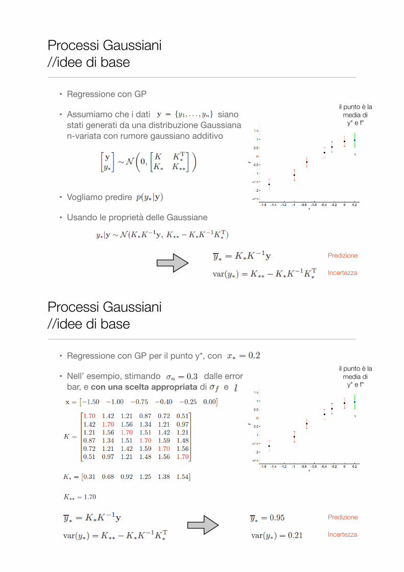
• Regressione con GP
• Assumiamo che i dati siano stati generati da una distribuzione Gaussiana n-variata con rumore gaussiano additivo
• Vogliamo predire
• Usando le proprietà delle Gaussiane
il punto è la media di
y* e f*
Predizione
Incertezza
Processi Gaussiani //idee di base
• Regressione con GP per il punto y*, con
• Nell’ esempio, stimando dalle error bar, e con una scelta appropriata di e
il punto è la media di
y* e f*
Predizione
Incertezza
Processi Gaussiani //idee di base
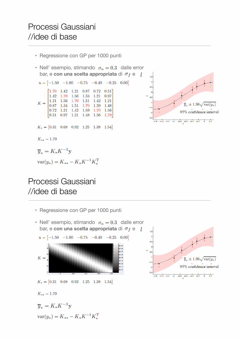
• Regressione con GP per 1000 punti
• Nell’ esempio, stimando dalle error bar, e con una scelta appropriata di e
Processi Gaussiani //idee di base
• Regressione con GP per 1000 punti
• Nell’ esempio, stimando dalle error bar, e con una scelta appropriata di e
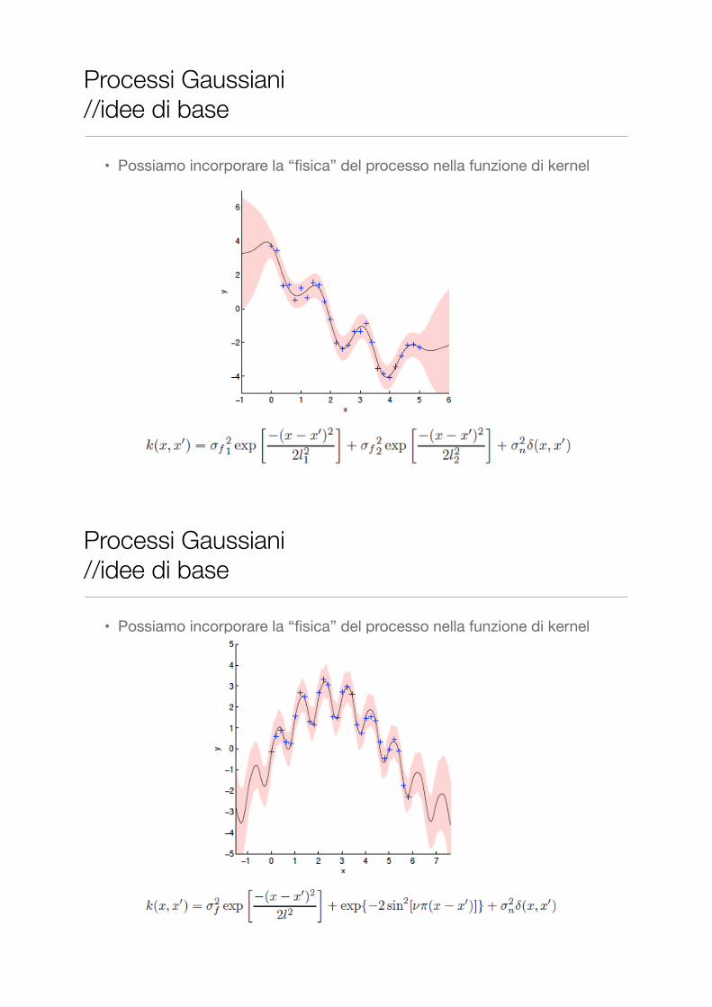
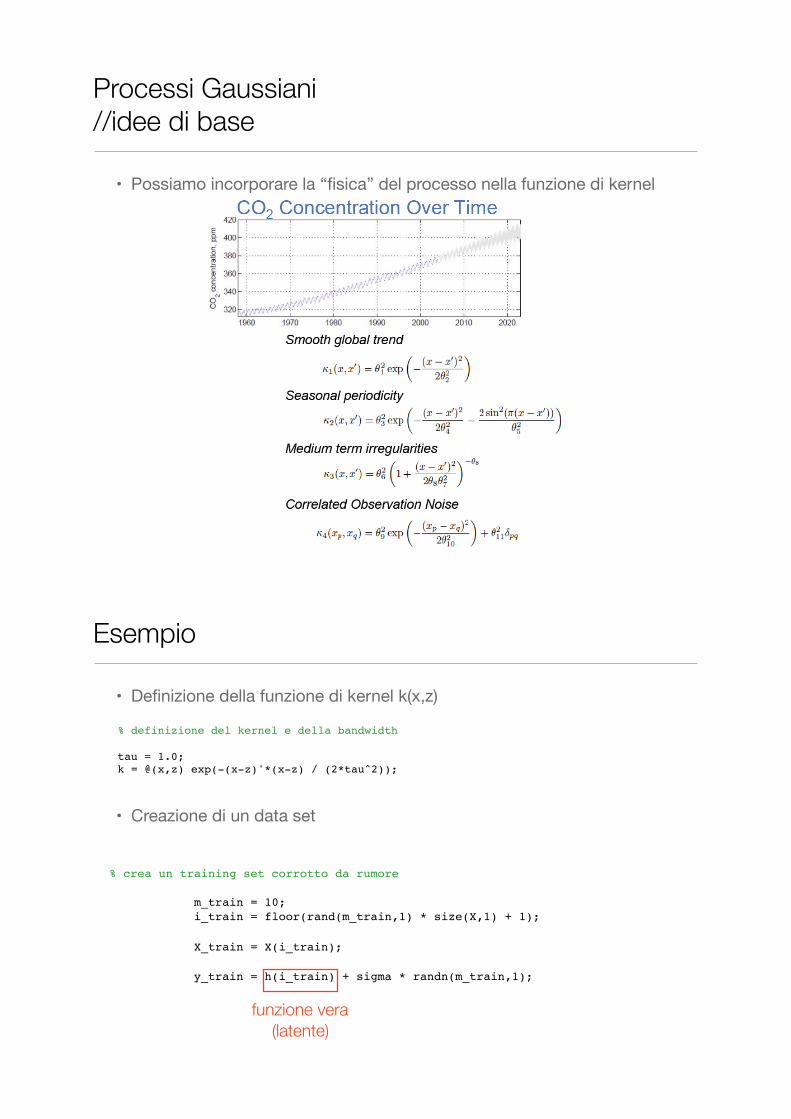
• Possiamo incorporare la “fisica” del processo nella funzione di kernel
Processi Gaussiani //idee di base
• Possiamo incorporare la “fisica” del processo nella funzione di kernel
Processi Gaussiani //idee di base
• Possiamo incorporare la “fisica” del processo nella funzione di kernel
Processi Gaussiani //idee di base
Esempio
• Definizione della funzione di kernel k(x,z)
• Creazione di un data set
% definizione del kernel e della bandwidth tau = 1.0;k = @(x,z) exp(-(x-z)'*(x-z) / (2*tau^2));
% crea un training set corrotto da rumore m_train = 10; i_train = floor(rand(m_train,1) * size(X,1) + 1);
X_train = X(i_train);
y_train = h(i_train) + sigma * randn(m_train,1);
funzione vera (latente)
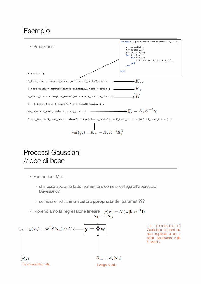
Esempio
• Predizione:
X_test = X;
K_test_test = compute_kernel_matrix(k,X_test,X_test);
K_test_train = compute_kernel_matrix(k,X_test,X_train);
K_train_train = compute_kernel_matrix(k,X_train,X_train);
G = K_train_train + sigma^2 * eye(size(X_train,1));
mu_test = K_test_train * (G \ y_train);
Sigma_test = K_test_test + sigma^2 * eye(size(X_test,1)) - K_test_train * (G \ (K_test_train'));
function [K] = compute_kernel_matrix(k, X, Z)
m = size(X,1);
n = size(Z,1); K = zeros(m,n); for i = 1:m
for j = 1:n K(i,j) = k(X(i,:)', Z(j,:)');
end end
end
• Fantastico! Ma...
• che cosa abbiamo fatto realmente e come si collega all’approccio Bayesiano?
• come si effettua una scelta appropriata dei parametri??
• Riprendiamo la regressione lineare
Processi Gaussiani //idee di base
L a p r o b a b i l i t à Gaussiana a priori sui pesi equivale a un a priori Gaussiano sulle funzioni y
Design MatrixCongiunta Normale
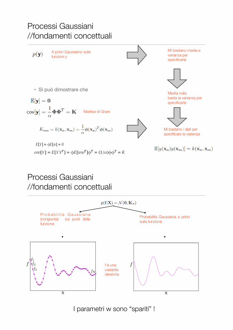
• Si può dimostrare che
Matrice di Gram
A priori Gaussiano sulle funzioni y
Mi bastano media e varianza per specificarla
Media nulla basta la varianza per specificarla
Mi bastano i dati per specificare la varianza
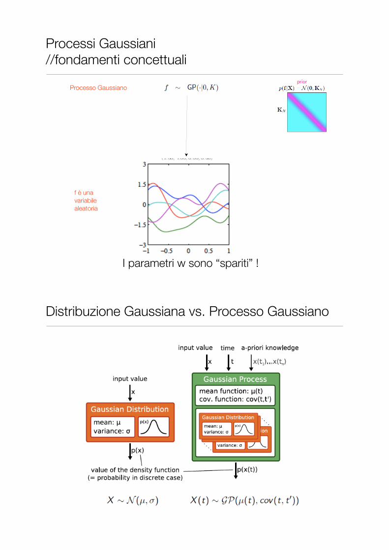
Processi Gaussiani //fondamenti concettuali
P r o b a b i l i t à G a u s s i a n a (congiunta) sui punti della funzione
Probabilità Gaussiana a priori sulla funzione
I parametri w sono “spariti” !
f è una variabile aleatoria
Processi Gaussiani //fondamenti concettuali
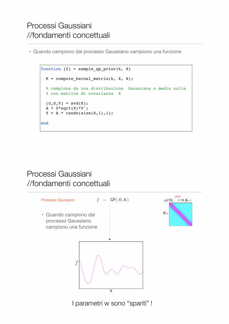
function [f] = sample_gp_prior(k, X) K = compute_kernel_matrix(k, X, X); % campiona da una distribuzione Gaussiana a media nulla % con matrice di covarianza K [U,S,V] = svd(K); A = U*sqrt(S)*V'; f = A * randn(size(X,1),1); end
Processi Gaussiani //fondamenti concettuali
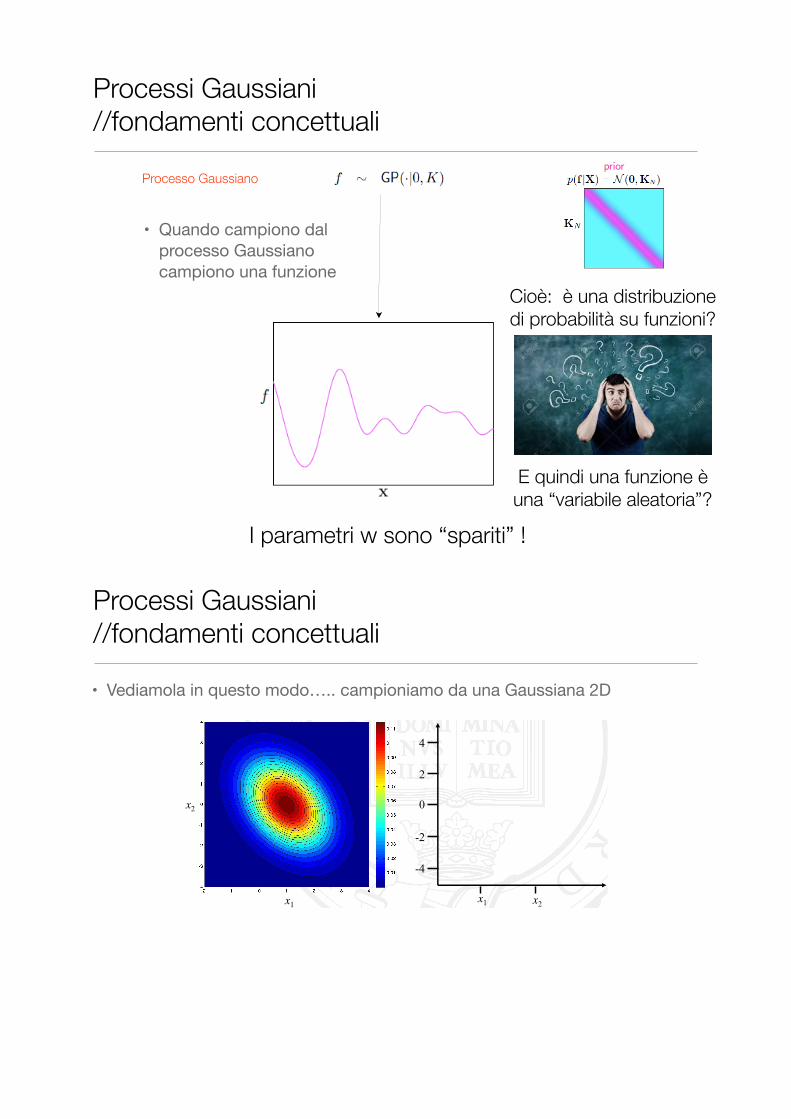
• Quando campiono dal processo Gaussiano campiono una funzione
Processo Gaussiano
I parametri w sono “spariti” !
Processi Gaussiani //fondamenti concettuali
• Quando campiono dal processo Gaussiano campiono una funzione
Processo Gaussiano
I parametri w sono “spariti” !
Processi Gaussiani //fondamenti concettuali
Cioè: è una distribuzione di probabilità su funzioni?
E quindi una funzione è una “variabile aleatoria”?
• Quando campiono dal processo Gaussiano campiono una funzione
Processi Gaussiani //fondamenti concettuali
• Vediamola in questo modo….. campioniamo da una Gaussiana 2D
� …which we can plot in a “horizontal manner”, if we wish
x1 x2 x1
x2 0
2
4
-2
-4
Processi Gaussiani //fondamenti concettuali
� …which we can plot in a “horizontal manner”, if we wish
x1 x2 x1
x2 0
2
4
-2
-4
� …which we can plot in a “horizontal manner”, if we wish
� …and where we can display a 2-D point using both plots
x1 x2 x1
x2 0
2
4
-2
-4
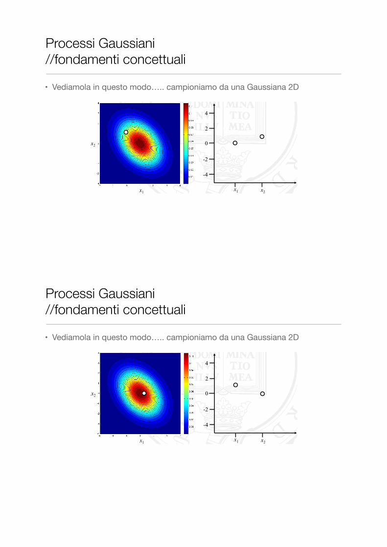
• Vediamola in questo modo….. campioniamo da una Gaussiana 2D
Processi Gaussiani //fondamenti concettuali
� …which we can plot in a “horizontal manner”, if we wish
x1 x2 x1
x2 0
2
4
-2
-4
� …which we can plot in a “horizontal manner”, if we wish
� …and where we can display a 2-D point using both plots
x1 x2 x1
x2 0
2
4
-2
-4
� …which we can plot in a “horizontal manner”, if we wish
� …and where we can display a 2-D point using both plots
x1 x2 x1
x2 0
2
4
-2
-4
• Vediamola in questo modo….. campioniamo da una Gaussiana 2D
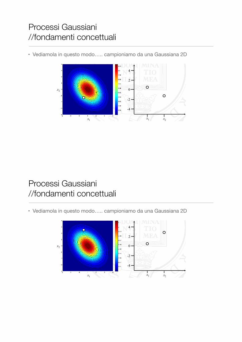
Processi Gaussiani //fondamenti concettuali
� …which we can plot in a “horizontal manner”, if we wish
x1 x2 x1
x2 0
2
4
-2
-4
� …which we can plot in a “horizontal manner”, if we wish
� …and where we can display a 2-D point using both plots
x1 x2 x1
x2 0
2
4
-2
-4
� …which we can plot in a “horizontal manner”, if we wish
� …and where we can display a 2-D point using both plots
x1 x2 x1
x2 0
2
4
-2
-4
� …which we can plot in a “horizontal manner”, if we wish
� …and where we can display a 2-D point using both plots
x1 x2 x1
x2 0
2
4
-2
-4
• Vediamola in questo modo….. campioniamo da una Gaussiana 2D
Processi Gaussiani //fondamenti concettuali
� …which we can plot in a “horizontal manner”, if we wish
x1 x2 x1
x2 0
2
4
-2
-4
� …which we can plot in a “horizontal manner”, if we wish
� …and where we can display a 2-D point using both plots
x1 x2 x1
x2 0
2
4
-2
-4
� …which we can plot in a “horizontal manner”, if we wish
� …and where we can display a 2-D point using both plots
x1 x2 x1
x2 0
2
4
-2
-4
� …which we can plot in a “horizontal manner”, if we wish
� …and where we can display a 2-D point using both plots
x1 x2 x1
x2 0
2
4
-2
-4
� …which we can plot in a “horizontal manner”, if we wish
� …and where we can display a 2-D point using both plots
x1 x2 x1
x2 0
2
4
-2
-4
• Vediamola in questo modo….. campioniamo da una Gaussiana 2D
Processi Gaussiani //fondamenti concettuali
� …which we can plot in a “horizontal manner”, if we wish
x1 x2 x1
x2 0
2
4
-2
-4
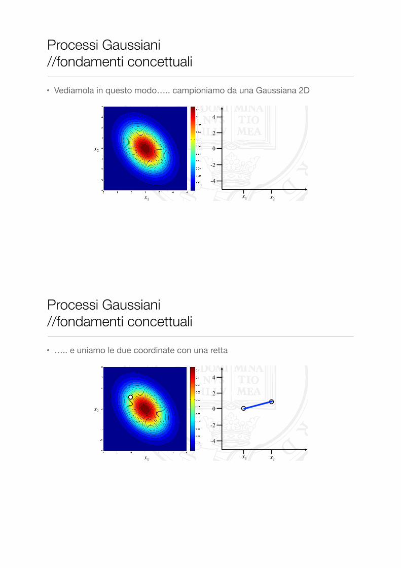
• Vediamola in questo modo….. campioniamo da una Gaussiana 2D
Processi Gaussiani //fondamenti concettuali
• ….. e uniamo le due coordinate con una retta
� …which we can plot in a “horizontal manner”, if we wish
x1 x2 x1
x2 0
2
4
-2
-4
� …which we can plot in a “horizontal manner”, if we wish
� …and where we can display a 2-D point using both plots
x1 x2 x1
x2 0
2
4
-2
-4
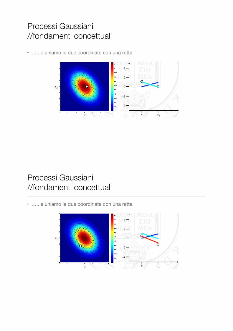
Processi Gaussiani //fondamenti concettuali
� …which we can plot in a “horizontal manner”, if we wish
x1 x2 x1
x2 0
2
4
-2
-4
� …which we can plot in a “horizontal manner”, if we wish
� …and where we can display a 2-D point using both plots
x1 x2 x1
x2 0
2
4
-2
-4
� …which we can plot in a “horizontal manner”, if we wish
� …and where we can display a 2-D point using both plots
x1 x2 x1
x2 0
2
4
-2
-4
• ….. e uniamo le due coordinate con una retta
Processi Gaussiani //fondamenti concettuali
� …which we can plot in a “horizontal manner”, if we wish
x1 x2 x1
x2 0
2
4
-2
-4
� …which we can plot in a “horizontal manner”, if we wish
� …and where we can display a 2-D point using both plots
x1 x2 x1
x2 0
2
4
-2
-4
� …which we can plot in a “horizontal manner”, if we wish
� …and where we can display a 2-D point using both plots
x1 x2 x1
x2 0
2
4
-2
-4
� …which we can plot in a “horizontal manner”, if we wish
� …and where we can display a 2-D point using both plots
x1 x2 x1
x2 0
2
4
-2
-4
� …which we can plot in a “horizontal manner”, if we wish
� …and where we can display a 2-D point using both plots
x1 x2 x1
x2 0
2
4
-2
-4
• ….. e uniamo le due coordinate con una retta
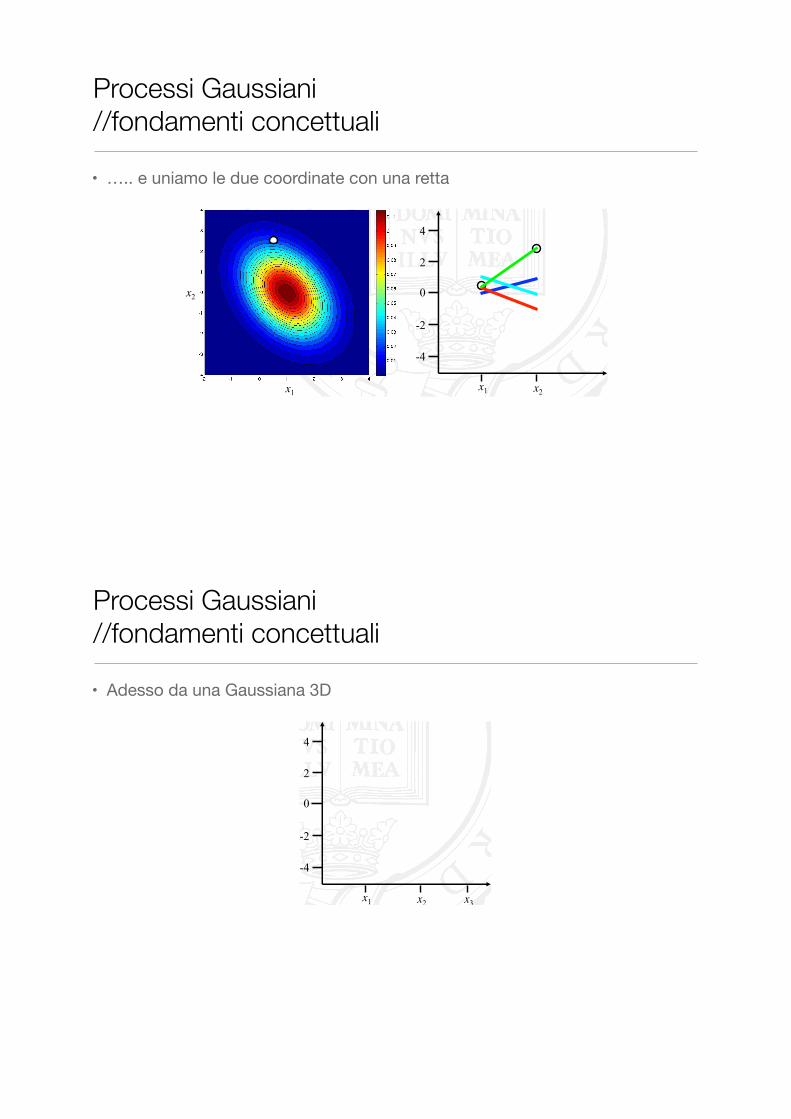
Processi Gaussiani //fondamenti concettuali
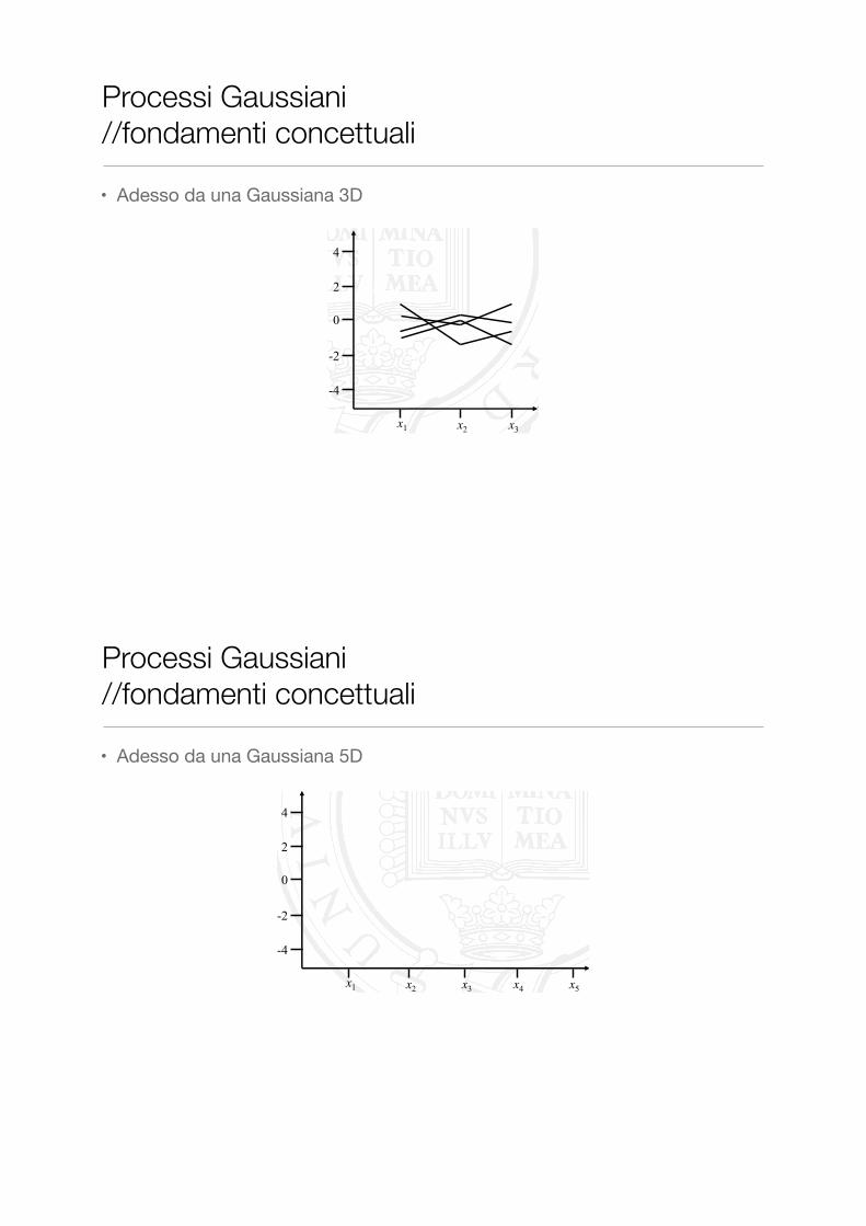
• Adesso da una Gaussiana 3D
� …but we’re not restricted to bivariate Gaussians
� Let’s introduce some extra dimensions, to our multivariate Gaussian distribution (without plotting it!)
� Perhaps unsurprisingly, as we generate points from our new trivariate distribution, we can equivalently show these on our three-column “horizontal” plot
x1 x2
0
2
4
-2
-4
x3
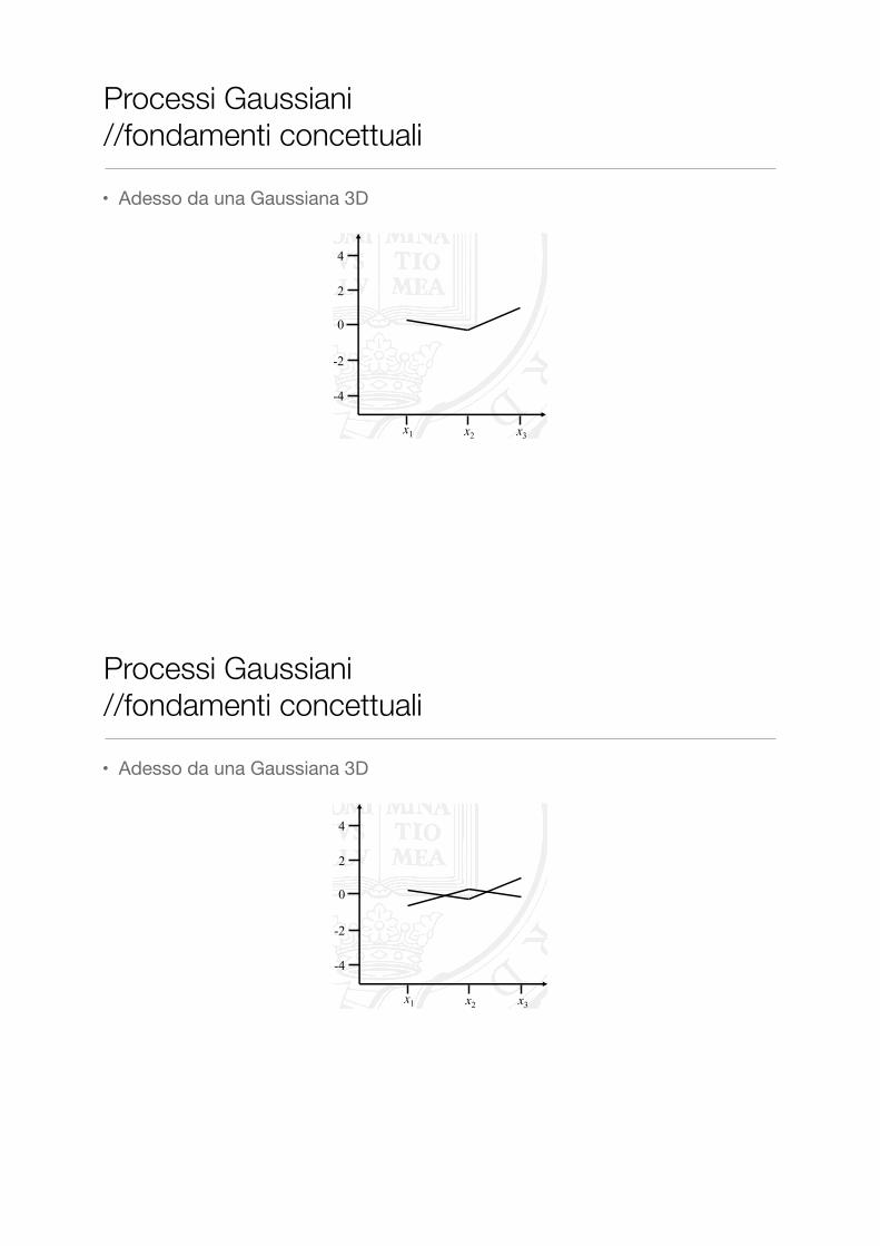
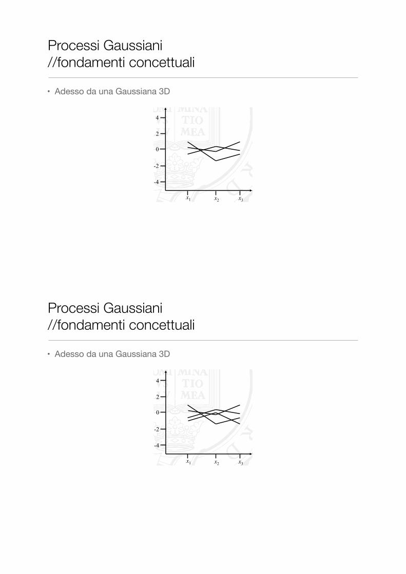
Processi Gaussiani //fondamenti concettuali
• Adesso da una Gaussiana 3D
� …but we’re not restricted to bivariate Gaussians
� Let’s introduce some extra dimensions, to our multivariate Gaussian distribution (without plotting it!)
� Perhaps unsurprisingly, as we generate points from our new trivariate distribution, we can equivalently show these on our three-column “horizontal” plot
x1 x2
0
2
4
-2
-4
x3
Processi Gaussiani //fondamenti concettuali
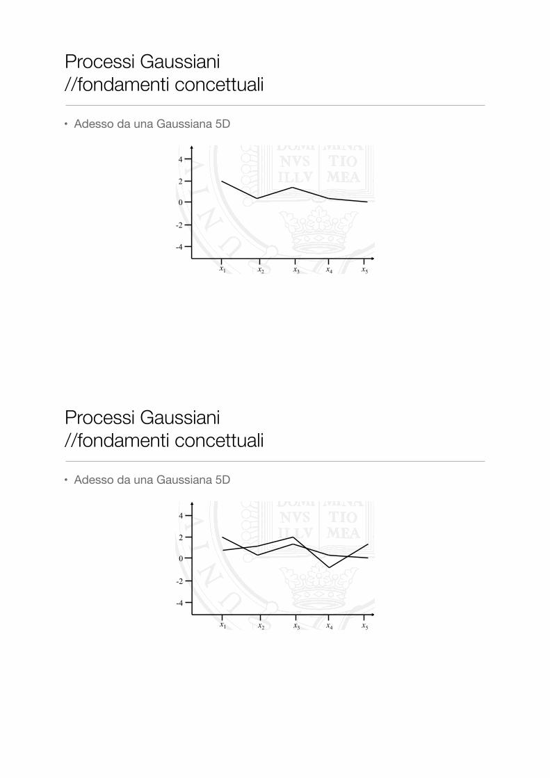
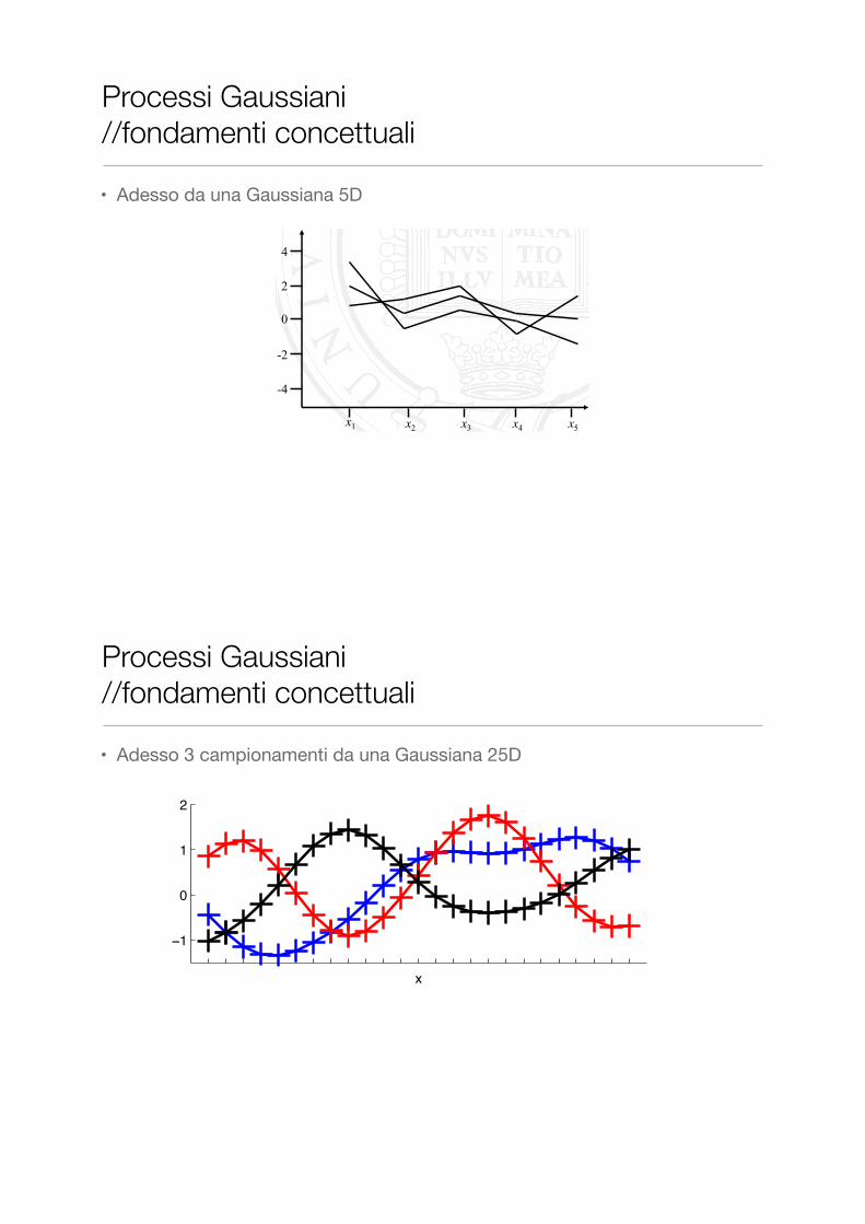
• Adesso da una Gaussiana 5D
� Why stop at a trivariate Gaussian distribution? We can add as many dimensions to our multivariate Gaussian as we wish
x1 x2
0
2
4
-2
-4
x3 x4 x5
Processi Gaussiani //fondamenti concettuali
• Adesso da una Gaussiana 5D
� Why stop at a trivariate Gaussian distribution? We can add as many dimensions to our multivariate Gaussian as we wish
x1 x2
0
2
4
-2
-4
x3 x4 x5
� Why stop at a trivariate Gaussian distribution? We can add as many dimensions to our multivariate Gaussian as we wish
x1 x2
0
2
4
-2
-4
x3 x4 x5
� Why stop at a trivariate Gaussian distribution? We can add as many dimensions to our multivariate Gaussian as we wish
x1 x2
0
2
4
-2
-4
x3 x4 x5
� Why stop at a trivariate Gaussian distribution? We can add as many dimensions to our multivariate Gaussian as we wish
x1 x2
0
2
4
-2
-4
x3 x4 x5
Processi Gaussiani //fondamenti concettuali
• Adesso 3 campionamenti da una Gaussiana 25DBuilding large Gaussians
Three draws from a 25D Gaussian:
−1
0
1
2
f
x
To produce this, we needed a mean: I used zeros(25,1)
The covariances were set using a kernel function: ⌃ij = k(xi,xj).
The x’s are the positions that I planted the tics on the axis.
Later we’ll find k’s that ensure ⌃ is always positive semi-definite.
Processo Gaussiano
I parametri w sono “spariti” !
f è una variabile aleatoria
Processi Gaussiani //fondamenti concettuali
Distribuzione Gaussiana vs. Processo Gaussiano
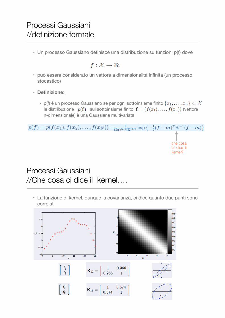
• Un processo Gaussiano definisce una distribuzione su funzioni p(f) dove
• può essere considerato un vettore a dimensionalità infinita (un processo stocastico)
• Definizione:
• p(f) è un processo Gaussiano se per ogni sottoinsieme finito la distribuzione sul sottoinsieme finito (vettore n-dimensionale) è una Gaussiana multivariata
Processi Gaussiani //definizione formale
che cosa ci dice il kernel?
• La funzione di kernel, dunque la covarianza, ci dice quanto due punti sono correlati
Processi Gaussiani //Che cosa ci dice il kernel….
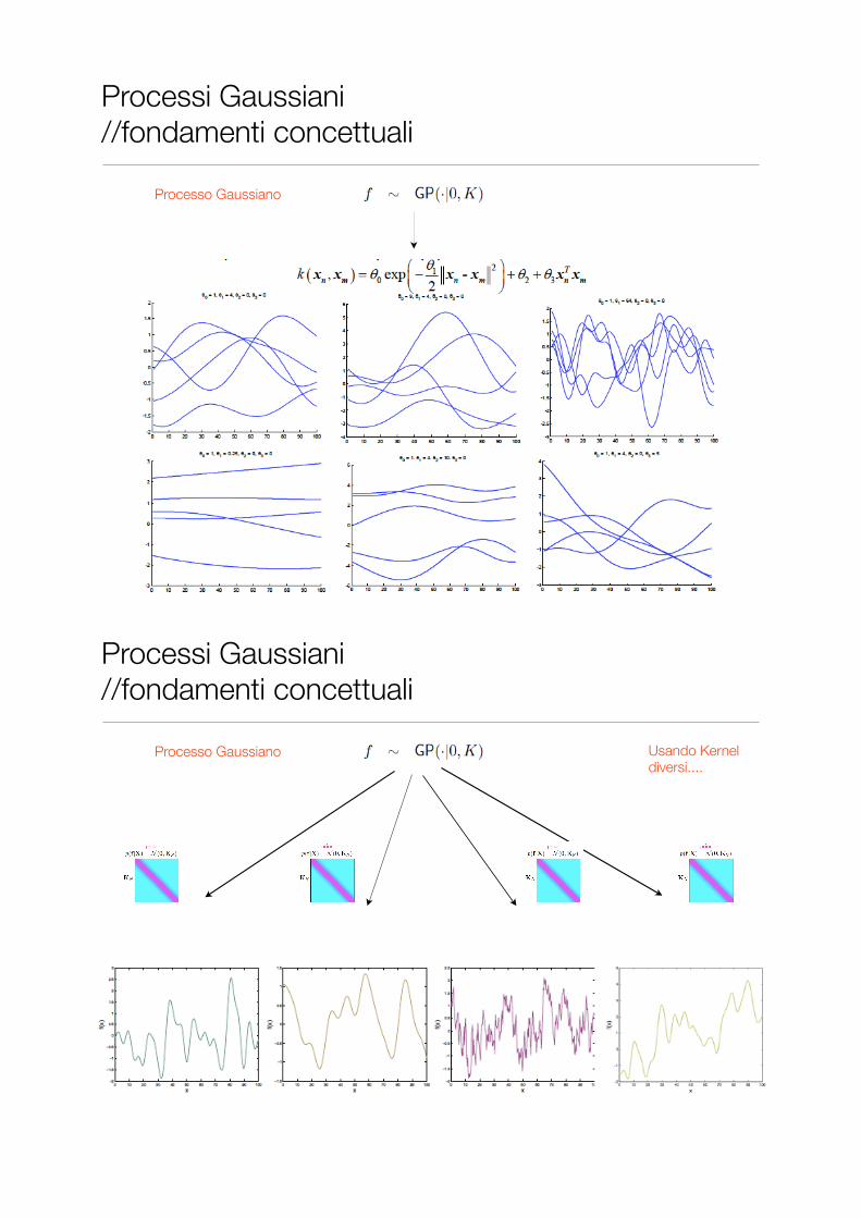
Processo Gaussiano
Processi Gaussiani //fondamenti concettuali
Processo Gaussiano Usando Kernel diversi....
Processi Gaussiani //fondamenti concettuali
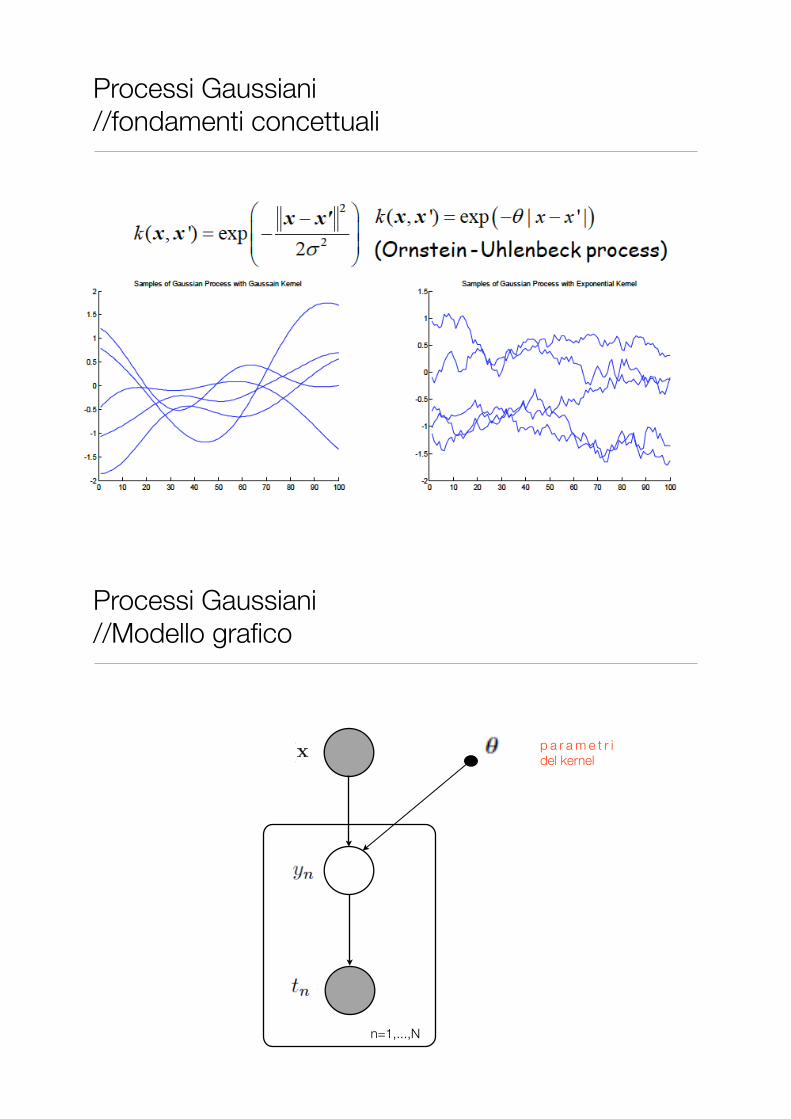
Processi Gaussiani //fondamenti concettuali
Processi Gaussiani //Modello grafico
n=1,...,N
p a r a m e t r i del kernel
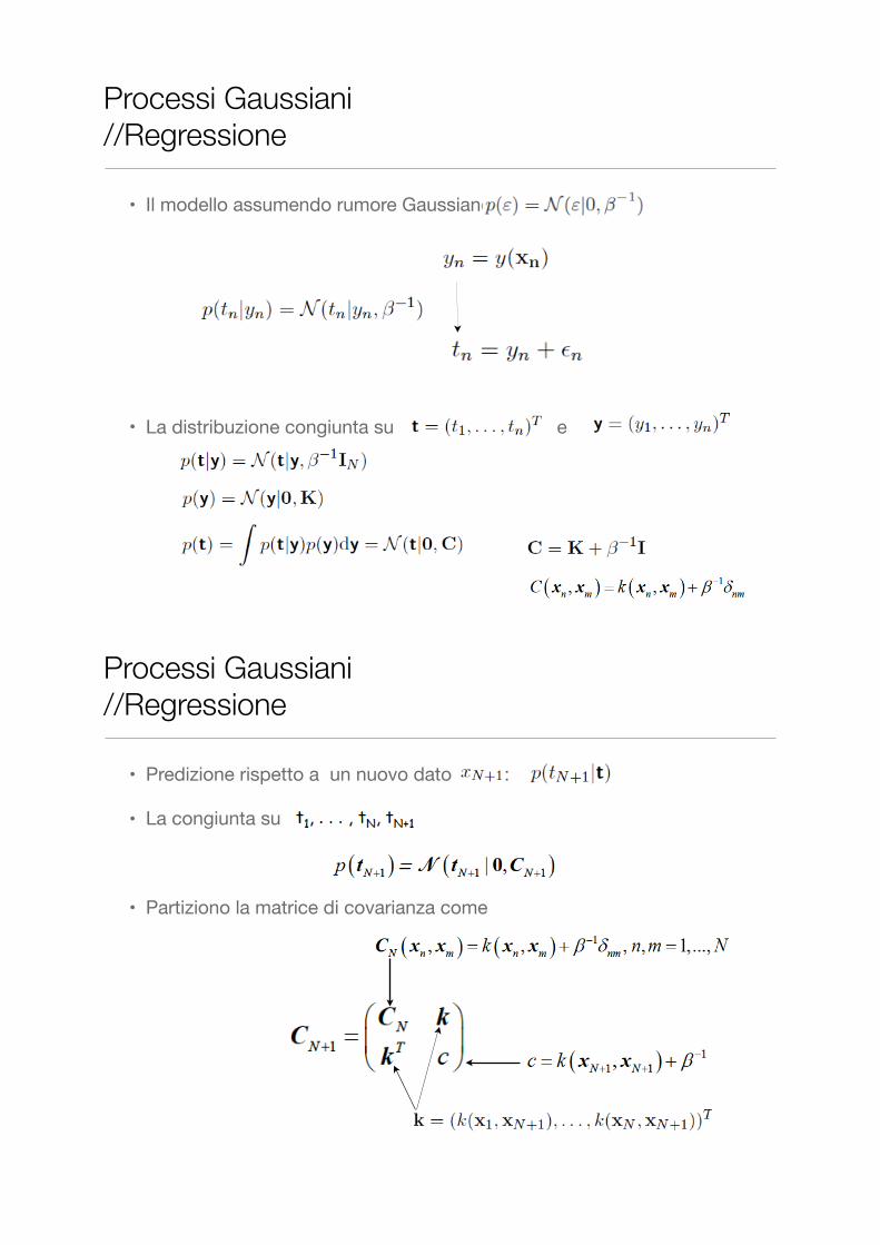
Processi Gaussiani //Regressione
• Il modello assumendo rumore Gaussiano
• La distribuzione congiunta su e
• Predizione rispetto a un nuovo dato :
• La congiunta su
• Partiziono la matrice di covarianza come
Processi Gaussiani //Regressione
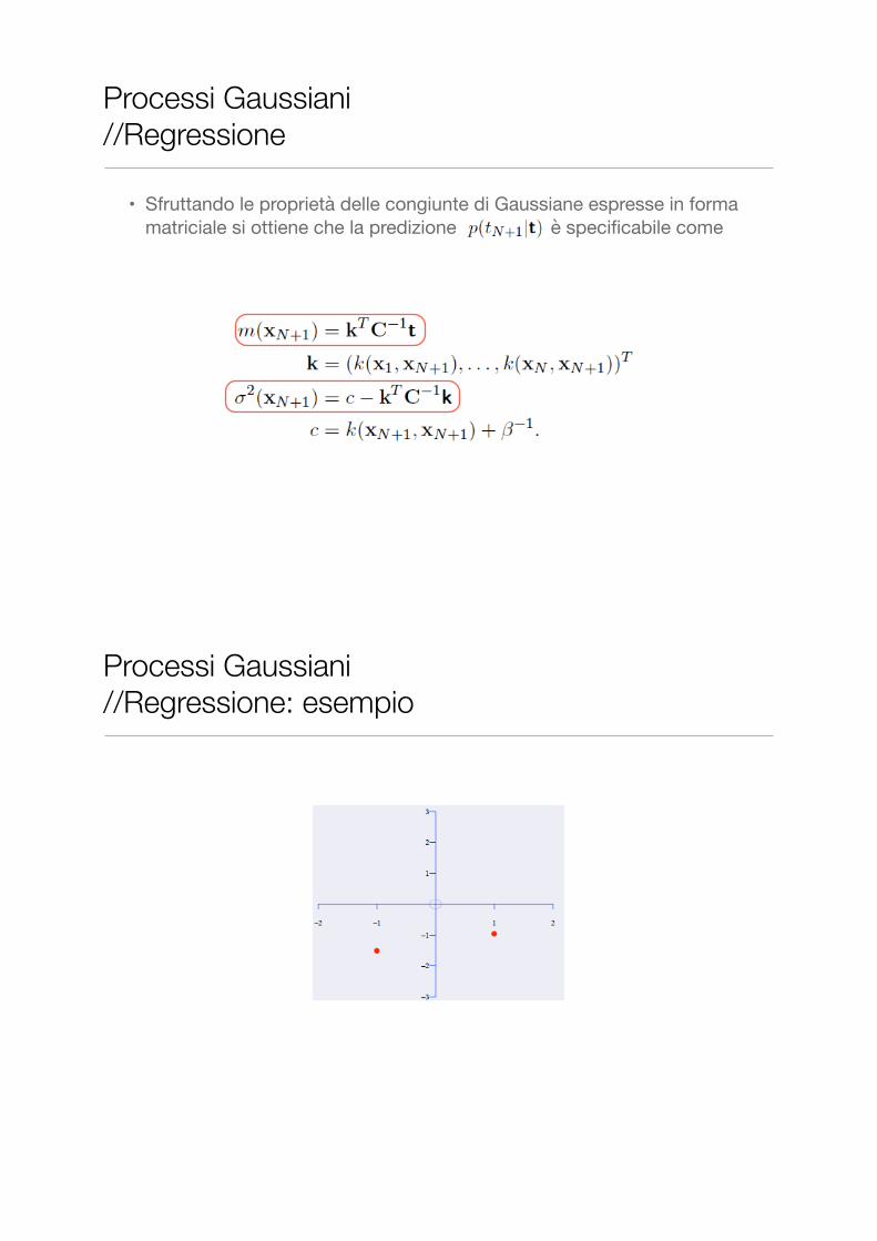
• Sfruttando le proprietà delle congiunte di Gaussiane espresse in forma matriciale si ottiene che la predizione è specificabile come
Processi Gaussiani //Regressione
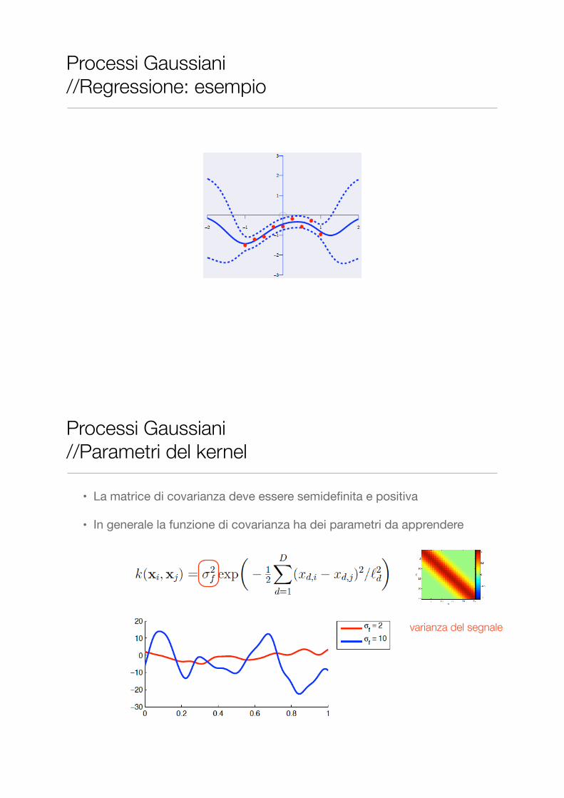
Processi Gaussiani //Regressione: esempio
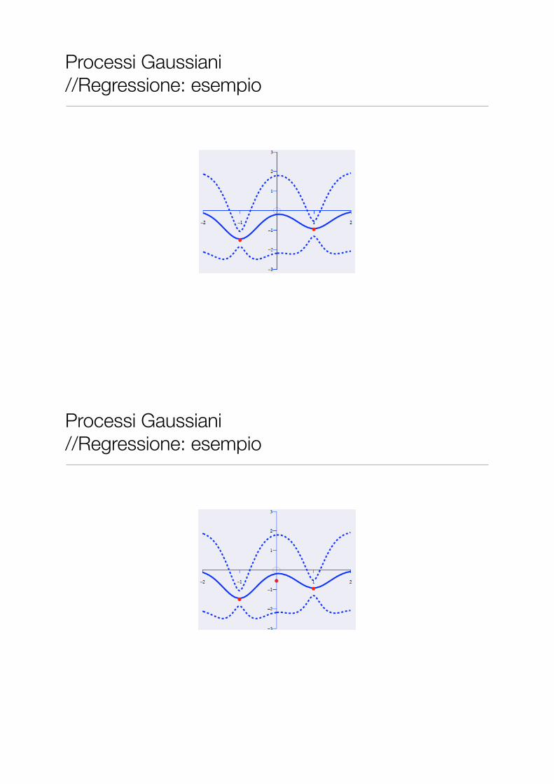
Processi Gaussiani //Regressione: esempio
Processi Gaussiani //Regressione: esempio
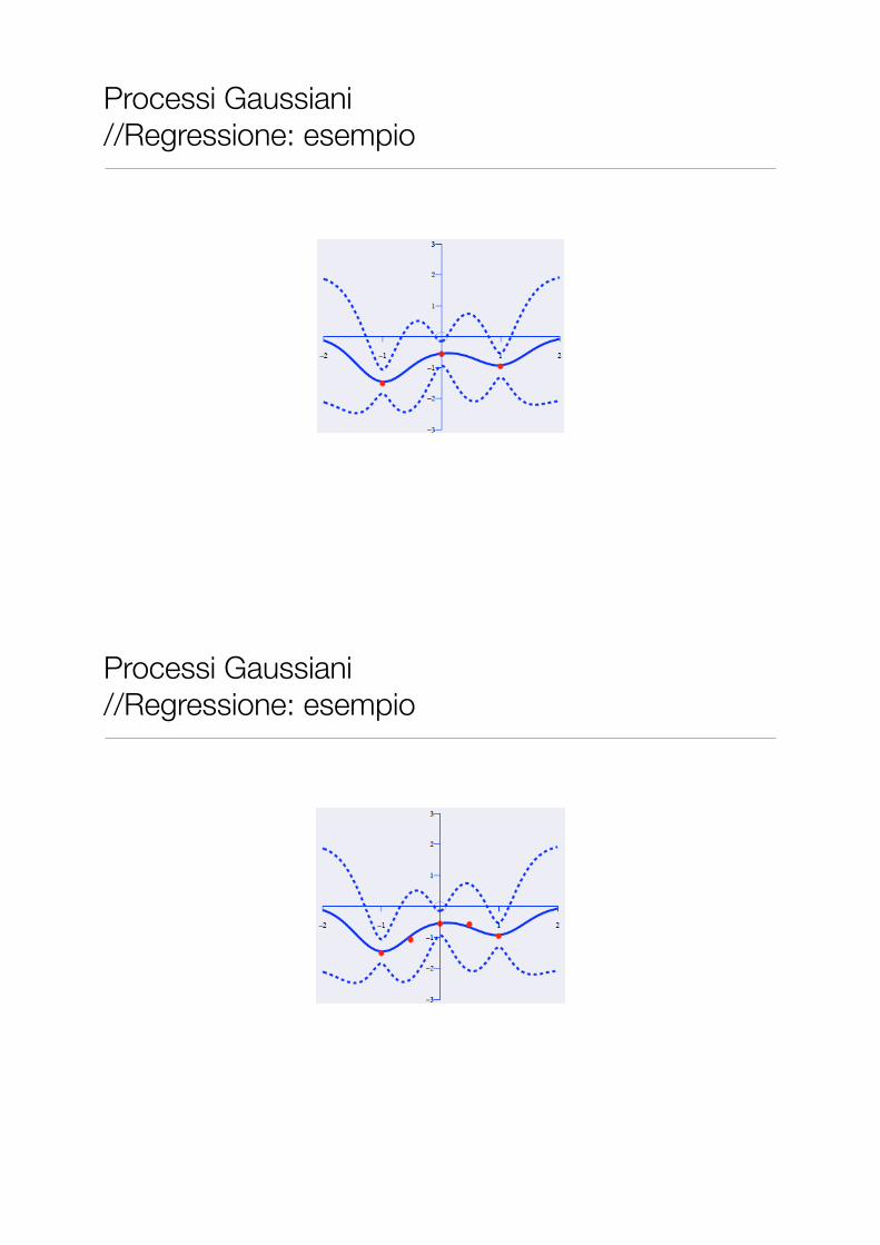
Processi Gaussiani //Regressione: esempio
Processi Gaussiani //Regressione: esempio
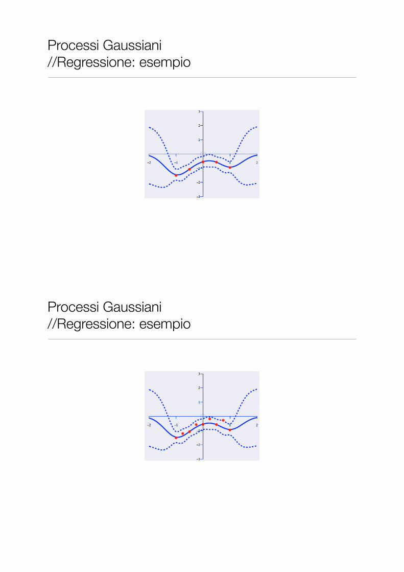
Processi Gaussiani //Regressione: esempio
Processi Gaussiani //Regressione: esempio
Processi Gaussiani //Regressione: esempio
• La matrice di covarianza deve essere semidefinita e positiva
• In generale la funzione di covarianza ha dei parametri da apprendere
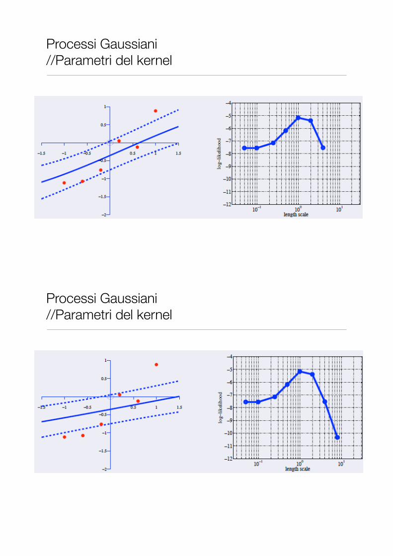
Processi Gaussiani //Parametri del kernel
varianza del segnale
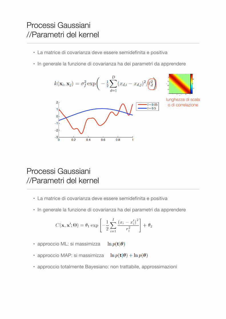
• La matrice di covarianza deve essere semidefinita e positiva
• In generale la funzione di covarianza ha dei parametri da apprendere
Processi Gaussiani //Parametri del kernel
lunghezza di scala o di correlazione
• La matrice di covarianza deve essere semidefinita e positiva
• In generale la funzione di covarianza ha dei parametri da apprendere
• approccio ML: si massimizza
• approccio MAP: si massimizza
• approccio totalmente Bayesiano: non trattabile, approssimazioni
Processi Gaussiani //Parametri del kernel
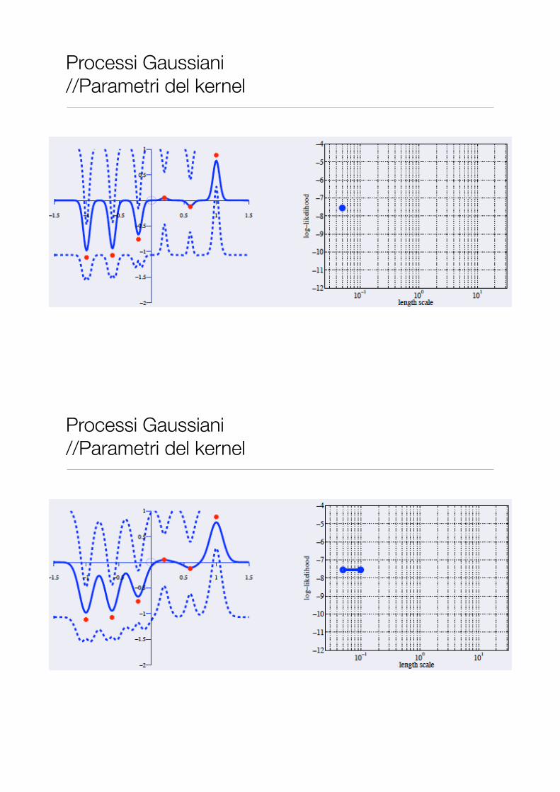
Processi Gaussiani //Parametri del kernel
Processi Gaussiani //Parametri del kernel

Processi Gaussiani //Parametri del kernel
Processi Gaussiani //Parametri del kernel
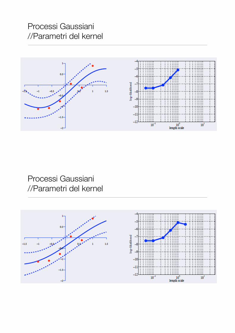
Processi Gaussiani //Parametri del kernel
Processi Gaussiani //Parametri del kernel
Processi Gaussiani //Parametri del kernel
Processi Gaussiani //Parametri del kernel