regionally accelerated batch informed trees …sanjibac/assets/docs/presentations/icra2016... ·...
TRANSCRIPT
air labRegionally Accelerated Batch Informed Trees (RABIT*):
A Framework to Integrate Local Information into Optimal Path Planning Sanjiban Choudhury1, Jonathan D. Gammell3,Timothy D. Barfoot3, Siddhartha S. Srinivasa2, and Sebastian Scherer1
1 2 3
(a) (b) (c)
x
goal
x
start
xk
x
goal
x
start
x
goal
x
start
xi xi
xj
xi
xj xj
xkxk
(a) (b) (c)
x
goal
x
start
xk
x
goal
x
start
x
goal
x
start
xi xi
xj
xi
xj xj
xkxk
(a) (b) (c)
x
goal
x
start
xk
x
goal
x
start
x
goal
x
start
xi xi
xj
xi
xj xj
xkxk
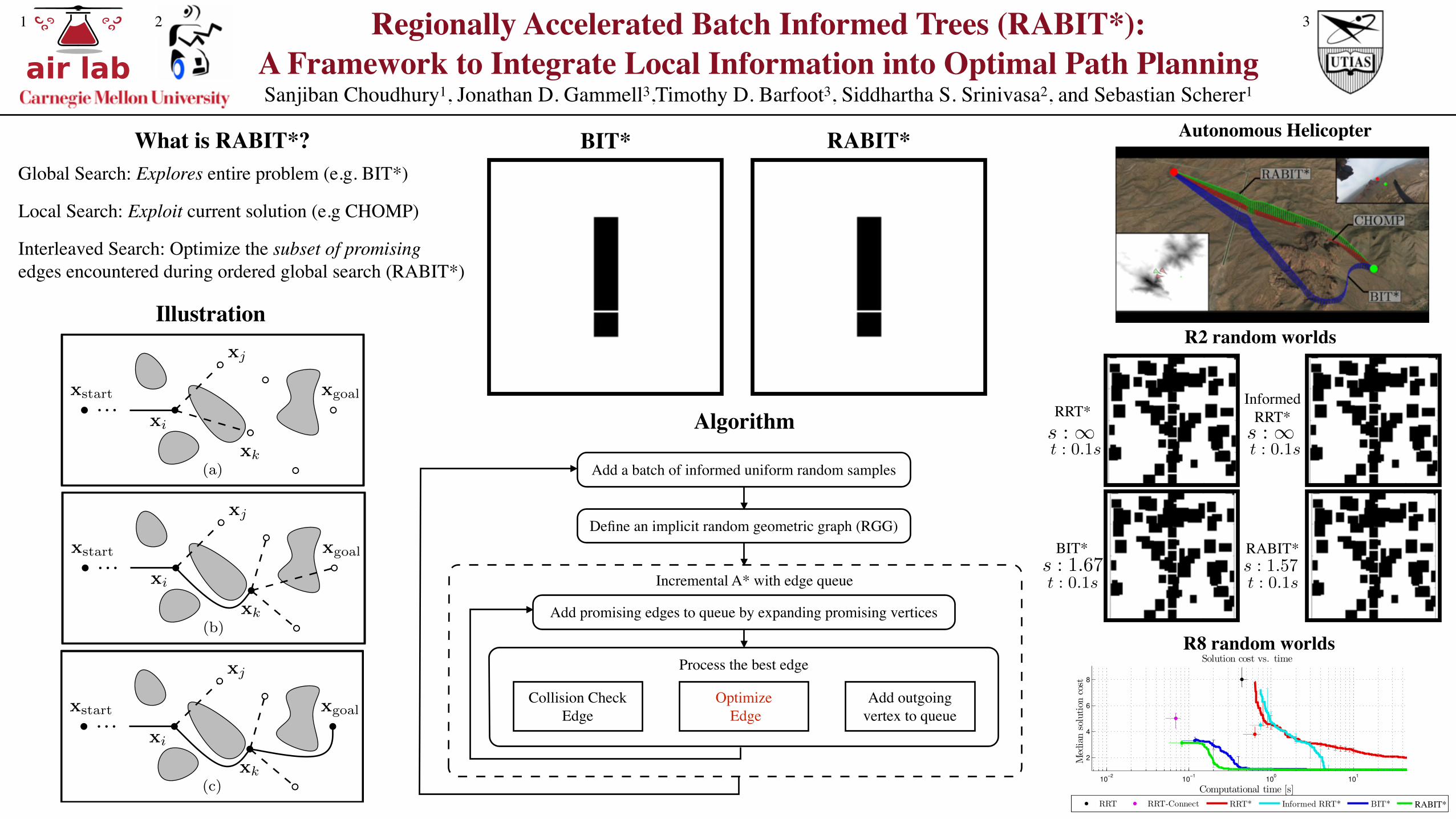
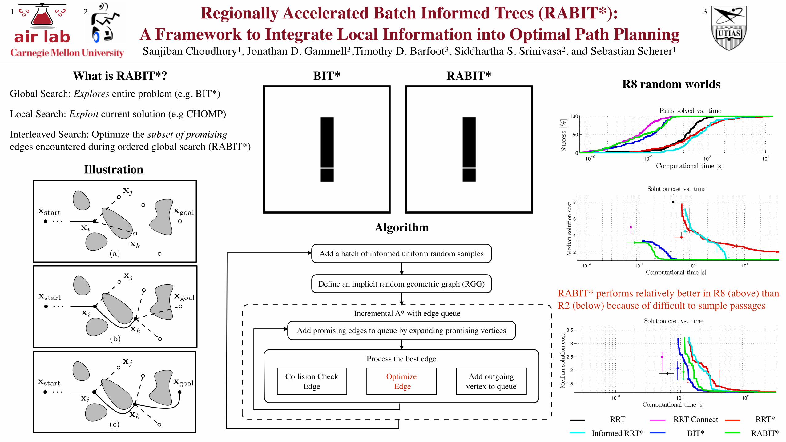
Algorithm
Add a batch of informed uniform random samples
Define an implicit random geometric graph (RGG)
Incremental A* with edge queue
Add promising edges to queue by expanding promising vertices
Process the best edge
Collision Check Edge
Optimize Edge
Add outgoing vertex to queue
What is RABIT*?
Interleaved Search: Optimize the subset of promising edges encountered during ordered global search (RABIT*)
Global Search: Explores entire problem (e.g. BIT*)
Local Search: Exploit current solution (e.g CHOMP)
Illustration
10−2
10−1
100
101
2
4
6
8
Computational time [s]
Solution cost vs. time
Med
ian
solu
tion
cost
RRT RRT-Connect RRT* Informed RRT* BIT* LOB*RABIT*
R8 random worlds
InformedRRT*RRT*
s : 1 s : 1
RABIT*s : 1.57
BIT*
R2 random worlds
t : 0.1s t : 0.1s
t : 0.1s t : 0.1ss : 1.67
Autonomous HelicopterBIT* RABIT*
air labRegionally Accelerated Batch Informed Trees (RABIT*):
A Framework to Integrate Local Information into Optimal Path Planning Sanjiban Choudhury1, Jonathan D. Gammell3,Timothy D. Barfoot3, Siddhartha S. Srinivasa2, and Sebastian Scherer1
1 2 3
(a) (b) (c)
x
goal
x
start
xk
x
goal
x
start
x
goal
x
start
xi xi
xj
xi
xj xj
xkxk
(a) (b) (c)
x
goal
x
start
xk
x
goal
x
start
x
goal
x
start
xi xi
xj
xi
xj xj
xkxk
(a) (b) (c)
x
goal
x
start
xk
x
goal
x
start
x
goal
x
start
xi xi
xj
xi
xj xj
xkxk
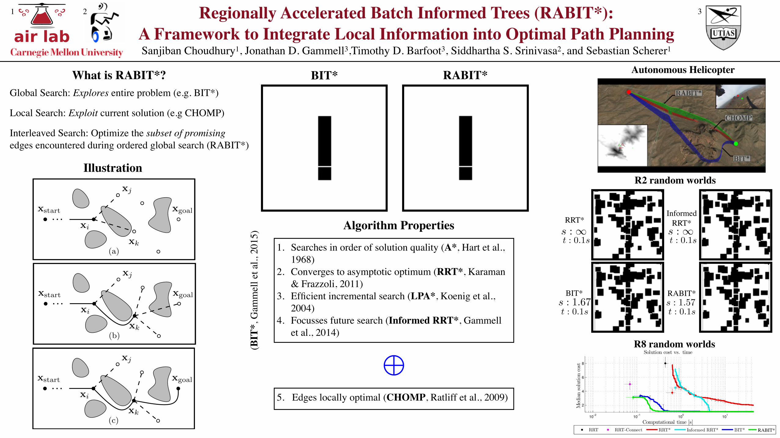
Algorithm Properties
What is RABIT*?
Interleaved Search: Optimize the subset of promising edges encountered during ordered global search (RABIT*)
Global Search: Explores entire problem (e.g. BIT*)
Local Search: Exploit current solution (e.g CHOMP)
Illustration
10−2
10−1
100
101
2
4
6
8
Computational time [s]
Solution cost vs. time
Med
ian
solu
tion
cost
RRT RRT-Connect RRT* Informed RRT* BIT* LOB*RABIT*
R8 random worlds
InformedRRT*RRT*
s : 1 s : 1
RABIT*s : 1.57
BIT*
R2 random worlds
t : 0.1s t : 0.1s
t : 0.1s t : 0.1ss : 1.67
Autonomous HelicopterBIT* RABIT*
1. Searches in order of solution quality (A*, Hart et al., 1968)
2. Converges to asymptotic optimum (RRT*, Karaman & Frazzoli, 2011)
3. Efficient incremental search (LPA*, Koenig et al., 2004)
4. Focusses future search (Informed RRT*, Gammell et al., 2014)
5. Edges locally optimal (CHOMP, Ratliff et al., 2009)
M(BIT
*, G
amm
ell e
t al.,
201
5)

air labRegionally Accelerated Batch Informed Trees (RABIT*):
A Framework to Integrate Local Information into Optimal Path Planning Sanjiban Choudhury1, Jonathan D. Gammell3,Timothy D. Barfoot3, Siddhartha S. Srinivasa2, and Sebastian Scherer1
1 2 3
(a) (b) (c)
x
goal
x
start
xk
x
goal
x
start
x
goal
x
start
xi xi
xj
xi
xj xj
xkxk
(a) (b) (c)
x
goal
x
start
xk
x
goal
x
start
x
goal
x
start
xi xi
xj
xi
xj xj
xkxk
(a) (b) (c)
x
goal
x
start
xk
x
goal
x
start
x
goal
x
start
xi xi
xj
xi
xj xj
xkxk
Algorithm
Illustration
10−2
10−1
100
101
2
4
6
8
Computational time [s]
Solution cost vs. time
Med
ian
solu
tion
cost
RRT RRT-Connect RRT* Informed RRT* BIT* LOB*RABIT*
R8 random worlds
InformedRRT*RRT*
s : 1 s : 1
RABIT*s : 1.57
BIT*
R2 random worlds
t : 0.1s t : 0.1s
t : 0.1s t : 0.1ss : 1.67
Autonomous HelicopterBIT* RABIT*
Algorithm 1: RABIT*�x
start
2 X
free
,x
goal
2 X
goal
�
1 V {xstart
} ; E ;; X
samples
�x
goal
;
2 QV ;; QE ��
x
start
,x
goal
� ; r 1;
3 repeat4 if QV ⌘ ; and QE ⌘ ; then5 Prune
�gT
�x
goal
��;
6 X
samples
+ � Sample�m, gT
�x
goal
��;
7 r radius�|V |+
��X
samples
���;8 QV V ;
9 while BestQueueValue (QV ) BestQueueValue (QE) do10 ExpandVertex (BestInQueue (QV ));
11 ProcessEdge (BestInQueue (QE));12 until STOP;13 return T ;
A. NotationWe define T := (V,E) to be an explicit tree with a set
of vertices, V ⇢ Xfree
, and edges, E = {(v,w)} for somev, w 2 V .
The functions bg (x) and bh (x) represent admissible es-timates of the cost-to-come to a state, x 2 X , from thestart and the cost-to-go from a state to the goal, respectively(i.e., they bound the true costs from below). The functiongT (x) represents the cost-to-come to a state, x 2 X , throughthe tree. We assume a state not in the tree has a cost-to-come of infinity. Note that these two functions will alwaysbound the unknown true optimal cost to a state, g (·), i.e.,8x 2 X, bg (x) g (x) gT (x).
There exists a path, �(v,w)
: [0, 1]! X , for every edge,(v,w), in the tree such that �
(v,w)
(0) = v and �(v,w)
(1) =w. The functions bs
��(v,w)
�and s
��(v,w)
�represents an
admissible estimate and the true cost of this path, respectively.With a slight abuse of notation, we denote the costs of straight-line edges as simply bs (v,w) and s (v,w).
Finally, the function � (·) represents the Lebesgue measureof a set (e.g., the volume), the cardinality of a set is denotedby |·|, and we take the minimum of an empty set to beinfinity, as is customary. We use the notation X
+ � {x}and X
� � {x} to compactly represent the compounding setoperations X X [ {x} and X X \ {x}, respectively.The trace of a matrix is given by tr (·) and the Euclideannorm of a vector or matrix is denoted by ||·||
2
. We use rand r to denote the vector and matrix gradients of a scalarfunction, respectively.
IV. ALGORITHM
We present RABIT*, a hybrid search technique. It generatesedges for a global search that avoid obstacles by using anoptimizer to exploit local domain information. It does thiswhile maintaining almost-sure asymptotic convergence to theglobal optimum.
The version presented uses CHOMP (Section IV-B) toexploit cost gradients inside BIT* (Section IV-A); however,other local optimization [34]–[36] or search techniques wouldalso be appropriate. CHOMP is a local optimization algorithmthat uses a quasi-Newton method to quickly improve a path byexploiting cost-gradient information. This not only improvesthe quality of the global search, but also its ability to finddifficult-to-sample homotopy classes.
Algorithm 2: ProcessEdge((vm
,x
m
) 2 QE)
1 QE� � {(v
m
,x
m
)};2 if gT (v
m
) + bs (vm
,x
m
) +
bh (x
m
) < gT�x
goal
�then
3 �
(vm,xm)
OptimizeEdge ((vm
,x
m
));4 if bg (v
m
) + s
��
(vm,xm)
�+
bh (x
m
) < gT�x
goal
�then
5 if gT (v
m
) + s
��
(vm,xm)
�< gT (x
m
) then6 if x
m
2 V then7 E
� � {(v,xm
) 2 E};
8 else9 X
samples
� � {xm
};10 V
+ � {xm
} ; QV+ � {x
m
};
11 E
+ � {(vm
,x
m
)};12 QE
� � {(v,xm
) 2 QE |gT (v) + bs (v,x
m
) � gT (x
m
)};
13 else14 QV ;; QE ;;
For simplicity, Algs. 1–4 present the search from a singlestart state to a single goal state. This formulation could easilybe extended to a goal region by extending the heuristic, orto a search originating from the goal.
A. Global SearchRABIT* uses the principles developed in BIT*. Due to
space constraints, we present only basic implementationdetails and direct the reader to [15] for more information.
BIT* is an asymptotically optimal planning algorithm thatorders its search on estimated solution cost and uses thecurrent solution to bound the search domain. This orderingprovides the opportunity to apply a local optimizer efficientlyin a global search. For clarity, we separate the algorithm intoa main section that is unchanged (Alg. 1) and the processingof edges (Alg. 2) where we highlight the changes in RABIT*.
The algorithm starts with a given initial state, xstart
2X
free
, in an otherwise empty tree, T . The goal state, xgoal
2X
goal
, is placed in the set of unconnected samples, Xsamples
,and the search queues are initialized (Alg. 1, Lines 1–2).
Whenever the queues are empty (Alg. 1, Line 4), RABIT*starts a new batch (Alg. 1, Lines 5–8). All vertices that cannotimprove the solution are removed (Alg. 1, Line 5, see [15])and more samples are added (Alg. 1, Line 6). This createsa new, denser implicit RGG from both the existing and newstates, defined by a connection radius, r (Alg. 1, Line 7). Theconnected vertices are then inserted into the vertex-expansionqueue to start the search (Alg. 1, Line 8).
The connection radius is calculated from bounds forasymptotic optimality [4],
radius (q) := 2⌘�1 + 1
n
� 1n
✓�(X bf)
⇣n
◆ 1n ⇣
log(q)q
⌘ 1n, (1)
where q is the number of vertices, X bf is the subset of statesthat can provide a better solution [5], ⇣n is the volume of ann-dimension unit ball, and ⌘ > 1 is a tuning parameter.
The underlying implicit RGG is searched in order ofdecreasing solution quality using a queue-based incrementalgraph search (Alg. 1, Lines 9–11) that expands vertices onlywhen necessary (Alg. 1, Lines 9–10). Vertices are expanded
Algorithm 3: OptimizeEdge((v,w) 2 QE)
1 if bs (v,w) < s (v,w) then2 �
0 Optimize ({v, w});3 if s (�0
) < s (v,w) then4 return �
0;
5 else6 return {v, w};
7 else8 return {v, w};
from a vertex queue, QV , into an edge queue, QE , whenthey could provide a better edge than the best of the edgequeue (Alg. 1, Line 9). The functions BestQueueValue andBestInQueue return the value of the best element and thebest element itself, respectively, for either the vertex or edgequeues. The ordering value of a vertex, v, or an edge, (v,x),in its queue is a lower bounding estimate of the cost of asolution constrained to pass through the vertex or edge giventhe current tree, gT (v)+bh (v), and gT (v)+bs (v,x)+bh (x),respectively. A vertex is expanded into the edge queue byadding the potential edges from the vertex to all other verticeswithin the distance r (Alg. 1, Line 10, see [15]).
As time allows, RABIT* processes the edge queue (Alg. 1,Line 11), increasing the density of the RGG with new batchesof samples when necessary.
Potential edges are processed by evaluating increasinglyaccurate cost calculations (Alg. 2). This allows optimizationsand collision checks to be delayed until necessary, limitingcomputational effort. The cost of a solution through the edgeis first estimated using an admissible estimate of the edgecost (Alg. 2, Line 2). If this cannot improve the currentsolution, then neither can the rest of the queue and the batchis finished (Alg. 2, Line 14). RABIT* then applies the localoptimizer in an attempt to find a collision-free path for theproposed edge (Alg. 2, Line 3, Section IV-B). The solutioncost through this path is then estimated using the actual pathcost (Alg. 2, Line 4). If this cannot improve the solution orit is in collision, then the potential edge is discarded. Finally,the effect of the path on the existing graph is evaluated, if itdoes not improve the cost-to-come of the target vertex thenit is discarded (Alg. 2, Line 5).
If the new path passes all these checks, it is added to thegraph as an edge (Alg. 2, Lines 6–12), either improving thepath to an existing state (a rewiring) or connecting a newstate (an expansion). For rewirings, the existing edge in thegraph is removed (Alg. 2, Line 7). For expansions, the vertexis moved from the set of unconnected samples and added tothe graph (Alg. 2, Lines 9–10). Finally, the queue is prunedof any redundant edges incoming to the vertex that cannotprovide a better path (Alg. 2, Line 12).
B. Local OptimizationLocal optimization is used to exploit domain information
to generate high-quality potential edges for the global search.Using obstacle information finds collision-free edges andhelps the global search find paths through difficult-to-samplehomotopy classes.
The integration of the local optimizer into the global
Algorithm 4: Optimize (�)
1 S
0 �;2 if ||� (1)� � (o)||
2
< � then3 if tr
⇣rc (S
0)
T rc (S
0)
⌘/c (S
0) � ⌫ then
4 for i = 0, 1, . . . , i
max
and ||rc (S
0)||
2
� " do5 �S �↵�1
i A
�1rc (S
0);
6 S
0 S
0+�S;
7 �
0 S
0;8 return �
0;
search is presented in Alg. 3. Edges are only optimizedif the heuristic predicts that a better path is possible (Alg. 3,Line 1), otherwise the original straight-line path is returned(Alg. 3, Line 8). If a better path may exist, the optimizeris applied to the straight-line edge between the two states(Alg. 3, Line 2). If the cost of the optimized path is lessthan the cost of the original, then the function returns theoptimized path (Alg. 3, Lines 3–4). If not, it returns thestraight-line path (Alg. 3, Line 6). This comparison allowsfor the integration of local optimization methods that do notguarantee obstacle avoidance or minimize a different costfunction (e.g., CHOMP) into the global search. Note that bydefinition, calculating the path cost includes collision checks.
1) Covariant Hamiltonian Optimization for Motion Plan-ning (CHOMP): In this version of RABIT*, we use CHOMPas a local optimizer to exploit cost gradients (Alg. 4). Dueto space constraints, we present only basic implementationdetails and direct the reader to [7] for more information,including on path parameterizations. We use a discretizedstraight-line parameterization to represent paths as matrices,S 2 Rz⇥n, where z is a number of intermediate waypointsbetween the start and end of the path, a single tuningparameter. These waypoints are internal to CHOMP and arenot considered vertices in the RABIT* graph.
To reduce optimization time, we skip paths that CHOMPcannot improve efficiently. To avoid low-resolution paths, weskip those longer than a user-tuned threshold (Alg. 4, Line 2).To avoid paths near local optima, we compare the trace of apaths cost gradient to its cost. If this ratio is insufficientlylarge, then the path is already near a local optima and isnot optimized further (Alg. 4, Line 3). The iterative CHOMPprocedure is then repeated for a specified number of iterations,imax
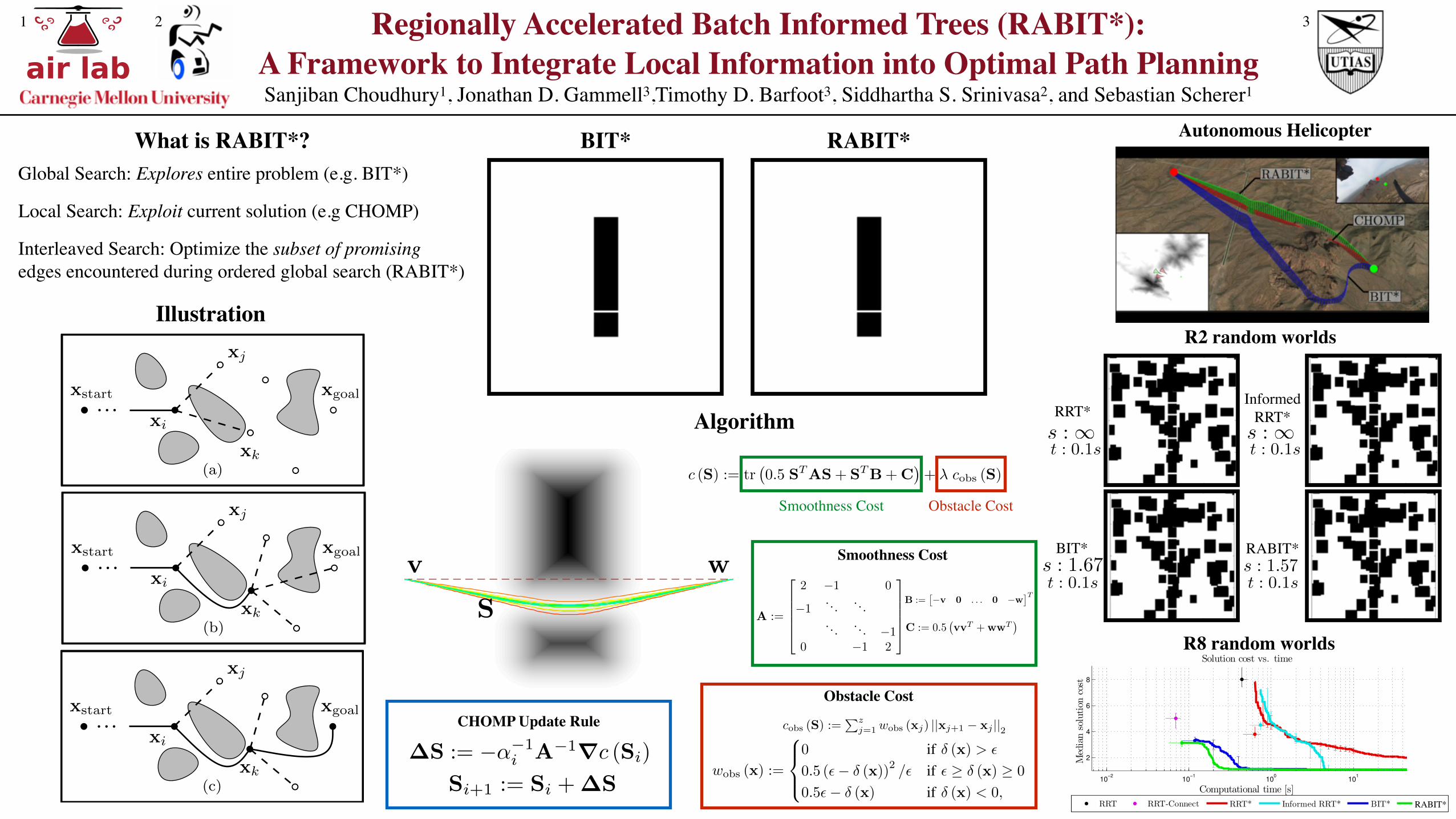
, while the gradient is sufficiently large (Alg. 4, Line 4).CHOMP minimizes a cost function, c (·) 2 R�0
, thatcombines path smoothness and obstacle avoidance,
c (S) := tr�0.5 S
TAS+ S
TB+C
�+ � c
obs
(S) ,
where � 2 R�0
is a user-tuned weighting parameter.The smoothness matrix terms, A 2 Rz⇥z , B 2 Rz⇥n, and
C 2 Rn⇥n are,
A :=
2
66664
2 �1 0
�1. . . . . .. . . . . . �1
0 �1 2
3
77775,
B :=⇥�v 0 . . . 0 �w
⇤T,
Algorithm 3: OptimizeEdge((v,w) 2 QE)
1 if bs (v,w) < s (v,w) then2 �
0 Optimize ({v, w});3 if s (�0
) < s (v,w) then4 return �
0;
5 else6 return {v, w};
7 else8 return {v, w};
from a vertex queue, QV , into an edge queue, QE , whenthey could provide a better edge than the best of the edgequeue (Alg. 1, Line 9). The functions BestQueueValue andBestInQueue return the value of the best element and thebest element itself, respectively, for either the vertex or edgequeues. The ordering value of a vertex, v, or an edge, (v,x),in its queue is a lower bounding estimate of the cost of asolution constrained to pass through the vertex or edge giventhe current tree, gT (v)+bh (v), and gT (v)+bs (v,x)+bh (x),respectively. A vertex is expanded into the edge queue byadding the potential edges from the vertex to all other verticeswithin the distance r (Alg. 1, Line 10, see [15]).
As time allows, RABIT* processes the edge queue (Alg. 1,Line 11), increasing the density of the RGG with new batchesof samples when necessary.
Potential edges are processed by evaluating increasinglyaccurate cost calculations (Alg. 2). This allows optimizationsand collision checks to be delayed until necessary, limitingcomputational effort. The cost of a solution through the edgeis first estimated using an admissible estimate of the edgecost (Alg. 2, Line 2). If this cannot improve the currentsolution, then neither can the rest of the queue and the batchis finished (Alg. 2, Line 14). RABIT* then applies the localoptimizer in an attempt to find a collision-free path for theproposed edge (Alg. 2, Line 3, Section IV-B). The solutioncost through this path is then estimated using the actual pathcost (Alg. 2, Line 4). If this cannot improve the solution orit is in collision, then the potential edge is discarded. Finally,the effect of the path on the existing graph is evaluated, if itdoes not improve the cost-to-come of the target vertex thenit is discarded (Alg. 2, Line 5).
If the new path passes all these checks, it is added to thegraph as an edge (Alg. 2, Lines 6–12), either improving thepath to an existing state (a rewiring) or connecting a newstate (an expansion). For rewirings, the existing edge in thegraph is removed (Alg. 2, Line 7). For expansions, the vertexis moved from the set of unconnected samples and added tothe graph (Alg. 2, Lines 9–10). Finally, the queue is prunedof any redundant edges incoming to the vertex that cannotprovide a better path (Alg. 2, Line 12).
B. Local OptimizationLocal optimization is used to exploit domain information
to generate high-quality potential edges for the global search.Using obstacle information finds collision-free edges andhelps the global search find paths through difficult-to-samplehomotopy classes.
The integration of the local optimizer into the global
Algorithm 4: Optimize (�)
1 S
0 �;2 if ||� (1)� � (o)||
2
< � then3 if tr
⇣rc (S
0)
T rc (S
0)
⌘/c (S
0) � ⌫ then
4 for i = 0, 1, . . . , i
max
and ||rc (S
0)||
2
� " do5 �S �↵�1
i A
�1rc (S
0);
6 S
0 S
0+�S;
7 �
0 S
0;8 return �
0;
search is presented in Alg. 3. Edges are only optimizedif the heuristic predicts that a better path is possible (Alg. 3,Line 1), otherwise the original straight-line path is returned(Alg. 3, Line 8). If a better path may exist, the optimizeris applied to the straight-line edge between the two states(Alg. 3, Line 2). If the cost of the optimized path is lessthan the cost of the original, then the function returns theoptimized path (Alg. 3, Lines 3–4). If not, it returns thestraight-line path (Alg. 3, Line 6). This comparison allowsfor the integration of local optimization methods that do notguarantee obstacle avoidance or minimize a different costfunction (e.g., CHOMP) into the global search. Note that bydefinition, calculating the path cost includes collision checks.
1) Covariant Hamiltonian Optimization for Motion Plan-ning (CHOMP): In this version of RABIT*, we use CHOMPas a local optimizer to exploit cost gradients (Alg. 4). Dueto space constraints, we present only basic implementationdetails and direct the reader to [7] for more information,including on path parameterizations. We use a discretizedstraight-line parameterization to represent paths as matrices,S 2 Rz⇥n, where z is a number of intermediate waypointsbetween the start and end of the path, a single tuningparameter. These waypoints are internal to CHOMP and arenot considered vertices in the RABIT* graph.
To reduce optimization time, we skip paths that CHOMPcannot improve efficiently. To avoid low-resolution paths, weskip those longer than a user-tuned threshold (Alg. 4, Line 2).To avoid paths near local optima, we compare the trace of apaths cost gradient to its cost. If this ratio is insufficientlylarge, then the path is already near a local optima and isnot optimized further (Alg. 4, Line 3). The iterative CHOMPprocedure is then repeated for a specified number of iterations,imax
, while the gradient is sufficiently large (Alg. 4, Line 4).CHOMP minimizes a cost function, c (·) 2 R�0
, thatcombines path smoothness and obstacle avoidance,
c (S) := tr�0.5 S
TAS+ S
TB+C
�+ � c
obs
(S) ,
where � 2 R�0
is a user-tuned weighting parameter.The smoothness matrix terms, A 2 Rz⇥z , B 2 Rz⇥n, and
C 2 Rn⇥n are,
A :=
2
66664
2 �1 0
�1. . . . . .. . . . . . �1
0 �1 2
3
77775,
B :=⇥�v 0 . . . 0 �w
⇤T,
What is RABIT*?
Interleaved Search: Optimize the subset of promising edges encountered during ordered global search (RABIT*)
Global Search: Explores entire problem (e.g. BIT*)
Local Search: Exploit current solution (e.g CHOMP)
air labRegionally Accelerated Batch Informed Trees (RABIT*):
A Framework to Integrate Local Information into Optimal Path Planning Sanjiban Choudhury1, Jonathan D. Gammell3,Timothy D. Barfoot3, Siddhartha S. Srinivasa2, and Sebastian Scherer1
1 2 3
(a) (b) (c)
x
goal
x
start
xk
x
goal
x
start
x
goal
x
start
xi xi
xj
xi
xj xj
xkxk
(a) (b) (c)
x
goal
x
start
xk
x
goal
x
start
x
goal
x
start
xi xi
xj
xi
xj xj
xkxk
(a) (b) (c)
x
goal
x
start
xk
x
goal
x
start
x
goal
x
start
xi xi
xj
xi
xj xj
xkxk
Algorithm
Illustration
10−2
10−1
100
101
2
4
6
8
Computational time [s]
Solution cost vs. time
Med
ian
solu
tion
cost
RRT RRT-Connect RRT* Informed RRT* BIT* LOB*RABIT*
R8 random worlds
InformedRRT*RRT*
s : 1 s : 1
RABIT*s : 1.57
BIT*
R2 random worlds
t : 0.1s t : 0.1s
t : 0.1s t : 0.1ss : 1.67
Autonomous HelicopterBIT* RABIT*
v w
S
Algorithm 3: OptimizeEdge((v,w) 2 QE)
1 if bs (v,w) < s (v,w) then2 �
0 Optimize ({v, w});3 if s (�0
) < s (v,w) then4 return �
0;
5 else6 return {v, w};
7 else8 return {v, w};
from a vertex queue, QV , into an edge queue, QE , whenthey could provide a better edge than the best of the edgequeue (Alg. 1, Line 9). The functions BestQueueValue andBestInQueue return the value of the best element and thebest element itself, respectively, for either the vertex or edgequeues. The ordering value of a vertex, v, or an edge, (v,x),in its queue is a lower bounding estimate of the cost of asolution constrained to pass through the vertex or edge giventhe current tree, gT (v)+bh (v), and gT (v)+bs (v,x)+bh (x),respectively. A vertex is expanded into the edge queue byadding the potential edges from the vertex to all other verticeswithin the distance r (Alg. 1, Line 10, see [15]).
As time allows, RABIT* processes the edge queue (Alg. 1,Line 11), increasing the density of the RGG with new batchesof samples when necessary.
Potential edges are processed by evaluating increasinglyaccurate cost calculations (Alg. 2). This allows optimizationsand collision checks to be delayed until necessary, limitingcomputational effort. The cost of a solution through the edgeis first estimated using an admissible estimate of the edgecost (Alg. 2, Line 2). If this cannot improve the currentsolution, then neither can the rest of the queue and the batchis finished (Alg. 2, Line 14). RABIT* then applies the localoptimizer in an attempt to find a collision-free path for theproposed edge (Alg. 2, Line 3, Section IV-B). The solutioncost through this path is then estimated using the actual pathcost (Alg. 2, Line 4). If this cannot improve the solution orit is in collision, then the potential edge is discarded. Finally,the effect of the path on the existing graph is evaluated, if itdoes not improve the cost-to-come of the target vertex thenit is discarded (Alg. 2, Line 5).
If the new path passes all these checks, it is added to thegraph as an edge (Alg. 2, Lines 6–12), either improving thepath to an existing state (a rewiring) or connecting a newstate (an expansion). For rewirings, the existing edge in thegraph is removed (Alg. 2, Line 7). For expansions, the vertexis moved from the set of unconnected samples and added tothe graph (Alg. 2, Lines 9–10). Finally, the queue is prunedof any redundant edges incoming to the vertex that cannotprovide a better path (Alg. 2, Line 12).
B. Local OptimizationLocal optimization is used to exploit domain information
to generate high-quality potential edges for the global search.Using obstacle information finds collision-free edges andhelps the global search find paths through difficult-to-samplehomotopy classes.
The integration of the local optimizer into the global
Algorithm 4: Optimize (�)
1 S
0 �;2 if ||� (1)� � (o)||
2
< � then3 if tr
⇣rc (S
0)
T rc (S
0)
⌘/c (S
0) � ⌫ then
4 for i = 0, 1, . . . , i
max
and ||rc (S
0)||
2
� " do5 �S �↵�1
i A
�1rc (S
0);
6 S
0 S
0+�S;
7 �
0 S
0;8 return �
0;
search is presented in Alg. 3. Edges are only optimizedif the heuristic predicts that a better path is possible (Alg. 3,Line 1), otherwise the original straight-line path is returned(Alg. 3, Line 8). If a better path may exist, the optimizeris applied to the straight-line edge between the two states(Alg. 3, Line 2). If the cost of the optimized path is lessthan the cost of the original, then the function returns theoptimized path (Alg. 3, Lines 3–4). If not, it returns thestraight-line path (Alg. 3, Line 6). This comparison allowsfor the integration of local optimization methods that do notguarantee obstacle avoidance or minimize a different costfunction (e.g., CHOMP) into the global search. Note that bydefinition, calculating the path cost includes collision checks.
1) Covariant Hamiltonian Optimization for Motion Plan-ning (CHOMP): In this version of RABIT*, we use CHOMPas a local optimizer to exploit cost gradients (Alg. 4). Dueto space constraints, we present only basic implementationdetails and direct the reader to [7] for more information,including on path parameterizations. We use a discretizedstraight-line parameterization to represent paths as matrices,S 2 Rz⇥n, where z is a number of intermediate waypointsbetween the start and end of the path, a single tuningparameter. These waypoints are internal to CHOMP and arenot considered vertices in the RABIT* graph.
To reduce optimization time, we skip paths that CHOMPcannot improve efficiently. To avoid low-resolution paths, weskip those longer than a user-tuned threshold (Alg. 4, Line 2).To avoid paths near local optima, we compare the trace of apaths cost gradient to its cost. If this ratio is insufficientlylarge, then the path is already near a local optima and isnot optimized further (Alg. 4, Line 3). The iterative CHOMPprocedure is then repeated for a specified number of iterations,imax
, while the gradient is sufficiently large (Alg. 4, Line 4).CHOMP minimizes a cost function, c (·) 2 R�0
, thatcombines path smoothness and obstacle avoidance,
c (S) := tr�0.5 S
TAS+ S
TB+C
�+ � c
obs
(S) ,
where � 2 R�0
is a user-tuned weighting parameter.The smoothness matrix terms, A 2 Rz⇥z , B 2 Rz⇥n, and
C 2 Rn⇥n are,
A :=
2
66664
2 �1 0
�1. . . . . .. . . . . . �1
0 �1 2
3
77775,
B :=⇥�v 0 . . . 0 �w
⇤T,
Smoothness Cost Obstacle Cost
Obstacle Cost
and
C := 0.5�vv
T +ww
T�,
where v and w are the start and end states of the path,respectively.
The obstacle cost, cobs
(·) 2 R�0
, is
cobs
(S) :=Pz
j=1
wobs
(xj) ||xj+1
� xj ||2
,
where xj is the j-th waypoint on the discretized path andthe weight, w
obs
(x), is given by
wobs
(x) :=
8><
>:
0 if � (x) > ✏
0.5 (✏� � (x))2 /✏ if ✏ � � (x) � 0
0.5✏� � (x) if � (x) < 0,
where ✏ 2 R>0
is a tuning parameter defining obstacleclearance. The function � (x) is the distance from the stateto the nearest obstacle boundary and is negative when thestate is inside an obstacle.
The form of this cost function allows CHOMP to use aquasi-Newton approach to iteratively optimize the path,
Si+1
:= Si +�S,
where �S 2 Rz⇥n,
�S := �↵�1
i A
�1rc (Si) ,
and 8i = 1, 2, . . . , imax
, ↵i 2 R�0
are tuning parameters thatdefine the step size at each iteration, i, of the optimization.
The matrix gradient of the cost function, rc (S) 2 Rz⇥n,is given analytically by
rc (S) = AS+B+rcobs
(S) ,
where the j-th row of the obstacle cost, rcobs
(S) 2 Rz⇥n, is
rcobs
(S)j = rwobs
(xj)T ||xj+1
� xj ||2
+ wobs
(xj�1
)x
Tj � x
Tj�1
||xj � xj�1
||2
+ wobs
(xj)x
Tj+1
� x
Tj
||xj+1
� xj ||2
,
and the vector gradient of the weight, rwobs
(x) 2 Rn, is
rwobs
(x) =
8><
>:
0 if � (x) > ✏
�r� (x) (✏� � (x)) /✏ if ✏ � � (x) � 0
�r� (x) if � (x) < 0,
and r� (·) 2 Rn is the vector gradient of the distance functionwith respect to a state. In some planning applications, thisdistance function and its gradient can be calculated a priori.
V. EXPERIMENTAL RESULTS
An Open Motion Planning Library (OMPL) [41] implemen-tation of RABIT* was evaluated on both simulated randomworlds (Section V-A) and a real planning problem from anautonomous helicopter (Section V-B)1.
A. Random WorldsTo systemically evaluate RABIT*, it was run on randomly
generated worlds in R2 and R8. It was compared to publicly1Experiments were run on a MacBook Pro with 16 GB of RAM and an
Intel i7-4870HQ processor running a 64-bit version of Ubuntu 14.04.
available OMPL implementations of RRT, RRT-Connect [42],RRT*, Informed RRT*, and BIT*.
Algorithms used an RGG constant (⌘ in (1)) of 1.1 andapproximated � (X
free
) with � (X). RRT-based algorithmsused a goal bias of 5%, and a maximum edge length of 0.2and 1.25 in R2 and R8, respectively. BIT*-based algorithmsused 100 samples per batch, Euclidean distance for heuristics,and direct informed sampling [5]. Graph pruning was limitedto changes in the solution cost greater than 1% and we usedan approximately sorted queue as discussed in [15]. RABIT*uses CHOMP parameters of � = 100, ✏ = 0.05, z = 8,� = 0.05 (R2) or 0.2 (R8), ⌫ = 0.1, i
max
= 5, " = 1⇥10�3,and ↵i = i�1/2⇥10�3. The distance gradient was calculatedanalytically.
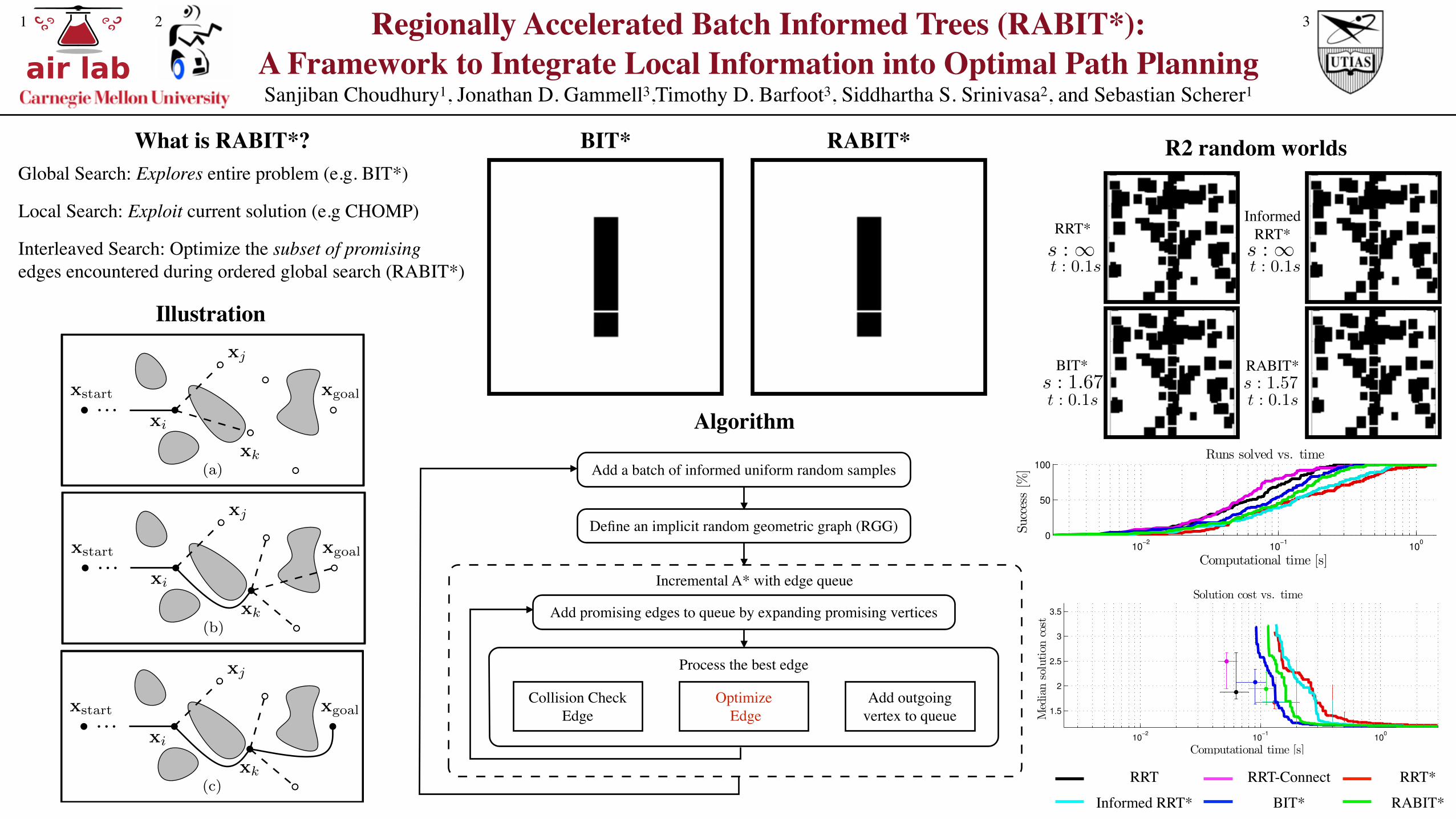
The worlds consisted of a (hyper)cube of width 2 dividedin half by a wall with 10 narrow gaps. The world alsocontained random axis-aligned (hyper)rectangular obstaclessuch that at most one third of the environment was obstructed.The start and goal states were located on different sidesof the wall at [�0.5, 0.0, . . . , 0.0] and [0.5, 0.0, . . . , 0.0],respectively (Fig. 3). This allowed us to randomly generatechallenging planning problems that had an optimal solutionpassing through a difficult-to-sample narrow passage.
For each state dimension, 10 different random worlds weregenerated and the planners were tested with 100 differentpseudo-random seeds on each world. The solution cost ofeach planner was recorded every 1 millisecond by a separatethread and the median was calculated by interpolating eachtrial at a period of 1 millisecond.
As the true optima for these problems are different andunknown, there is no meaningful way to compare theresults across problems. Instead, results from a representativeproblem are presented in Fig. 4, where the percent of trialssolved and the median solution cost are plotted versuscomputation time.
To quantify the results in Fig. 4, we calculate the timefor each algorithm to reach 90% of its final value. In R2,RABIT* takes 0.215s compared to BIT*’s 0.179s. In R8,RABIT* takes 0.262s compared to BIT*’s 0.471s.
These results show that in R2 RABIT* performs similarlyto BIT*; however, that in R8 RABIT* finds better solutionsfaster on these problems with difficult-to-sample homotopyclasses.
B. Autonomous HelicopterTo evaluate RABIT* on real planning problems, it was
run on a recorded flight mission of an autonomous helicopter.The autonomous helicopter operates at speeds of up to50 meters/second in challenging environments that maycontain difficult-to-sample features such as valleys. Plansmust obey the dynamic and power constraints of the vehicle(including climb-rate limits) and completely avoid obstacles,a planning problem that is difficult to solve in real time.
Sensor data collected from test flights over Mesa, Arizonawere used to propose a planning problem around mountains(Fig. 5). This problem is challenging because the helicopter’sconstraints create a large number of states from which no
and
C := 0.5�vv
T +ww
T�,
where v and w are the start and end states of the path,respectively.
The obstacle cost, cobs
(·) 2 R�0
, is
cobs
(S) :=Pz
j=1
wobs
(xj) ||xj+1
� xj ||2
,
where xj is the j-th waypoint on the discretized path andthe weight, w
obs
(x), is given by
wobs
(x) :=
8><
>:
0 if � (x) > ✏
0.5 (✏� � (x))2 /✏ if ✏ � � (x) � 0
0.5✏� � (x) if � (x) < 0,
where ✏ 2 R>0
is a tuning parameter defining obstacleclearance. The function � (x) is the distance from the stateto the nearest obstacle boundary and is negative when thestate is inside an obstacle.
The form of this cost function allows CHOMP to use aquasi-Newton approach to iteratively optimize the path,
Si+1
:= Si +�S,
where �S 2 Rz⇥n,
�S := �↵�1
i A
�1rc (Si) ,
and 8i = 1, 2, . . . , imax
, ↵i 2 R�0
are tuning parameters thatdefine the step size at each iteration, i, of the optimization.
The matrix gradient of the cost function, rc (S) 2 Rz⇥n,is given analytically by
rc (S) = AS+B+rcobs
(S) ,
where the j-th row of the obstacle cost, rcobs
(S) 2 Rz⇥n, is
rcobs
(S)j = rwobs
(xj)T ||xj+1
� xj ||2
+ wobs
(xj�1
)x
Tj � x
Tj�1
||xj � xj�1
||2
+ wobs
(xj)x
Tj+1
� x
Tj
||xj+1
� xj ||2
,
and the vector gradient of the weight, rwobs
(x) 2 Rn, is
rwobs
(x) =
8><
>:
0 if � (x) > ✏
�r� (x) (✏� � (x)) /✏ if ✏ � � (x) � 0
�r� (x) if � (x) < 0,
and r� (·) 2 Rn is the vector gradient of the distance functionwith respect to a state. In some planning applications, thisdistance function and its gradient can be calculated a priori.
V. EXPERIMENTAL RESULTS
An Open Motion Planning Library (OMPL) [41] implemen-tation of RABIT* was evaluated on both simulated randomworlds (Section V-A) and a real planning problem from anautonomous helicopter (Section V-B)1.
A. Random WorldsTo systemically evaluate RABIT*, it was run on randomly
generated worlds in R2 and R8. It was compared to publicly1Experiments were run on a MacBook Pro with 16 GB of RAM and an
Intel i7-4870HQ processor running a 64-bit version of Ubuntu 14.04.
available OMPL implementations of RRT, RRT-Connect [42],RRT*, Informed RRT*, and BIT*.
Algorithms used an RGG constant (⌘ in (1)) of 1.1 andapproximated � (X
free
) with � (X). RRT-based algorithmsused a goal bias of 5%, and a maximum edge length of 0.2and 1.25 in R2 and R8, respectively. BIT*-based algorithmsused 100 samples per batch, Euclidean distance for heuristics,and direct informed sampling [5]. Graph pruning was limitedto changes in the solution cost greater than 1% and we usedan approximately sorted queue as discussed in [15]. RABIT*uses CHOMP parameters of � = 100, ✏ = 0.05, z = 8,� = 0.05 (R2) or 0.2 (R8), ⌫ = 0.1, i
max
= 5, " = 1⇥10�3,and ↵i = i�1/2⇥10�3. The distance gradient was calculatedanalytically.
The worlds consisted of a (hyper)cube of width 2 dividedin half by a wall with 10 narrow gaps. The world alsocontained random axis-aligned (hyper)rectangular obstaclessuch that at most one third of the environment was obstructed.The start and goal states were located on different sidesof the wall at [�0.5, 0.0, . . . , 0.0] and [0.5, 0.0, . . . , 0.0],respectively (Fig. 3). This allowed us to randomly generatechallenging planning problems that had an optimal solutionpassing through a difficult-to-sample narrow passage.
For each state dimension, 10 different random worlds weregenerated and the planners were tested with 100 differentpseudo-random seeds on each world. The solution cost ofeach planner was recorded every 1 millisecond by a separatethread and the median was calculated by interpolating eachtrial at a period of 1 millisecond.
As the true optima for these problems are different andunknown, there is no meaningful way to compare theresults across problems. Instead, results from a representativeproblem are presented in Fig. 4, where the percent of trialssolved and the median solution cost are plotted versuscomputation time.
To quantify the results in Fig. 4, we calculate the timefor each algorithm to reach 90% of its final value. In R2,RABIT* takes 0.215s compared to BIT*’s 0.179s. In R8,RABIT* takes 0.262s compared to BIT*’s 0.471s.
These results show that in R2 RABIT* performs similarlyto BIT*; however, that in R8 RABIT* finds better solutionsfaster on these problems with difficult-to-sample homotopyclasses.
B. Autonomous HelicopterTo evaluate RABIT* on real planning problems, it was
run on a recorded flight mission of an autonomous helicopter.The autonomous helicopter operates at speeds of up to50 meters/second in challenging environments that maycontain difficult-to-sample features such as valleys. Plansmust obey the dynamic and power constraints of the vehicle(including climb-rate limits) and completely avoid obstacles,a planning problem that is difficult to solve in real time.
Sensor data collected from test flights over Mesa, Arizonawere used to propose a planning problem around mountains(Fig. 5). This problem is challenging because the helicopter’sconstraints create a large number of states from which no
Algorithm 3: OptimizeEdge((v,w) 2 QE)
1 if bs (v,w) < s (v,w) then2 �
0 Optimize ({v, w});3 if s (�0
) < s (v,w) then4 return �
0;
5 else6 return {v, w};
7 else8 return {v, w};
from a vertex queue, QV , into an edge queue, QE , whenthey could provide a better edge than the best of the edgequeue (Alg. 1, Line 9). The functions BestQueueValue andBestInQueue return the value of the best element and thebest element itself, respectively, for either the vertex or edgequeues. The ordering value of a vertex, v, or an edge, (v,x),in its queue is a lower bounding estimate of the cost of asolution constrained to pass through the vertex or edge giventhe current tree, gT (v)+bh (v), and gT (v)+bs (v,x)+bh (x),respectively. A vertex is expanded into the edge queue byadding the potential edges from the vertex to all other verticeswithin the distance r (Alg. 1, Line 10, see [15]).
As time allows, RABIT* processes the edge queue (Alg. 1,Line 11), increasing the density of the RGG with new batchesof samples when necessary.
Potential edges are processed by evaluating increasinglyaccurate cost calculations (Alg. 2). This allows optimizationsand collision checks to be delayed until necessary, limitingcomputational effort. The cost of a solution through the edgeis first estimated using an admissible estimate of the edgecost (Alg. 2, Line 2). If this cannot improve the currentsolution, then neither can the rest of the queue and the batchis finished (Alg. 2, Line 14). RABIT* then applies the localoptimizer in an attempt to find a collision-free path for theproposed edge (Alg. 2, Line 3, Section IV-B). The solutioncost through this path is then estimated using the actual pathcost (Alg. 2, Line 4). If this cannot improve the solution orit is in collision, then the potential edge is discarded. Finally,the effect of the path on the existing graph is evaluated, if itdoes not improve the cost-to-come of the target vertex thenit is discarded (Alg. 2, Line 5).
If the new path passes all these checks, it is added to thegraph as an edge (Alg. 2, Lines 6–12), either improving thepath to an existing state (a rewiring) or connecting a newstate (an expansion). For rewirings, the existing edge in thegraph is removed (Alg. 2, Line 7). For expansions, the vertexis moved from the set of unconnected samples and added tothe graph (Alg. 2, Lines 9–10). Finally, the queue is prunedof any redundant edges incoming to the vertex that cannotprovide a better path (Alg. 2, Line 12).
B. Local OptimizationLocal optimization is used to exploit domain information
to generate high-quality potential edges for the global search.Using obstacle information finds collision-free edges andhelps the global search find paths through difficult-to-samplehomotopy classes.
The integration of the local optimizer into the global
Algorithm 4: Optimize (�)
1 S
0 �;2 if ||� (1)� � (o)||
2
< � then3 if tr
⇣rc (S
0)
T rc (S
0)
⌘/c (S
0) � ⌫ then
4 for i = 0, 1, . . . , i
max
and ||rc (S
0)||
2
� " do5 �S �↵�1
i A
�1rc (S
0);
6 S
0 S
0+�S;
7 �
0 S
0;8 return �
0;
search is presented in Alg. 3. Edges are only optimizedif the heuristic predicts that a better path is possible (Alg. 3,Line 1), otherwise the original straight-line path is returned(Alg. 3, Line 8). If a better path may exist, the optimizeris applied to the straight-line edge between the two states(Alg. 3, Line 2). If the cost of the optimized path is lessthan the cost of the original, then the function returns theoptimized path (Alg. 3, Lines 3–4). If not, it returns thestraight-line path (Alg. 3, Line 6). This comparison allowsfor the integration of local optimization methods that do notguarantee obstacle avoidance or minimize a different costfunction (e.g., CHOMP) into the global search. Note that bydefinition, calculating the path cost includes collision checks.
1) Covariant Hamiltonian Optimization for Motion Plan-ning (CHOMP): In this version of RABIT*, we use CHOMPas a local optimizer to exploit cost gradients (Alg. 4). Dueto space constraints, we present only basic implementationdetails and direct the reader to [7] for more information,including on path parameterizations. We use a discretizedstraight-line parameterization to represent paths as matrices,S 2 Rz⇥n, where z is a number of intermediate waypointsbetween the start and end of the path, a single tuningparameter. These waypoints are internal to CHOMP and arenot considered vertices in the RABIT* graph.
To reduce optimization time, we skip paths that CHOMPcannot improve efficiently. To avoid low-resolution paths, weskip those longer than a user-tuned threshold (Alg. 4, Line 2).To avoid paths near local optima, we compare the trace of apaths cost gradient to its cost. If this ratio is insufficientlylarge, then the path is already near a local optima and isnot optimized further (Alg. 4, Line 3). The iterative CHOMPprocedure is then repeated for a specified number of iterations,imax
, while the gradient is sufficiently large (Alg. 4, Line 4).CHOMP minimizes a cost function, c (·) 2 R�0
, thatcombines path smoothness and obstacle avoidance,
c (S) := tr�0.5 S
TAS+ S
TB+C
�+ � c
obs
(S) ,
where � 2 R�0
is a user-tuned weighting parameter.The smoothness matrix terms, A 2 Rz⇥z , B 2 Rz⇥n, and
C 2 Rn⇥n are,
A :=
2
66664
2 �1 0
�1. . . . . .. . . . . . �1
0 �1 2
3
77775,
B :=⇥�v 0 . . . 0 �w
⇤T,
and
C := 0.5�vv
T +ww
T�,
where v and w are the start and end states of the path,respectively.
The obstacle cost, cobs
(·) 2 R�0
, is
cobs
(S) :=Pz
j=1
wobs
(xj) ||xj+1
� xj ||2
,
where xj is the j-th waypoint on the discretized path andthe weight, w
obs
(x), is given by
wobs
(x) :=
8><
>:
0 if � (x) > ✏
0.5 (✏� � (x))2 /✏ if ✏ � � (x) � 0
0.5✏� � (x) if � (x) < 0,
where ✏ 2 R>0
is a tuning parameter defining obstacleclearance. The function � (x) is the distance from the stateto the nearest obstacle boundary and is negative when thestate is inside an obstacle.
The form of this cost function allows CHOMP to use aquasi-Newton approach to iteratively optimize the path,
Si+1
:= Si +�S,
where �S 2 Rz⇥n,
�S := �↵�1
i A
�1rc (Si) ,
and 8i = 1, 2, . . . , imax
, ↵i 2 R�0
are tuning parameters thatdefine the step size at each iteration, i, of the optimization.
The matrix gradient of the cost function, rc (S) 2 Rz⇥n,is given analytically by
rc (S) = AS+B+rcobs
(S) ,
where the j-th row of the obstacle cost, rcobs
(S) 2 Rz⇥n, is
rcobs
(S)j = rwobs
(xj)T ||xj+1
� xj ||2
+ wobs
(xj�1
)x
Tj � x
Tj�1
||xj � xj�1
||2
+ wobs
(xj)x
Tj+1
� x
Tj
||xj+1
� xj ||2
,
and the vector gradient of the weight, rwobs
(x) 2 Rn, is
rwobs
(x) =
8><
>:
0 if � (x) > ✏
�r� (x) (✏� � (x)) /✏ if ✏ � � (x) � 0
�r� (x) if � (x) < 0,
and r� (·) 2 Rn is the vector gradient of the distance functionwith respect to a state. In some planning applications, thisdistance function and its gradient can be calculated a priori.
V. EXPERIMENTAL RESULTS
An Open Motion Planning Library (OMPL) [41] implemen-tation of RABIT* was evaluated on both simulated randomworlds (Section V-A) and a real planning problem from anautonomous helicopter (Section V-B)1.
A. Random WorldsTo systemically evaluate RABIT*, it was run on randomly
generated worlds in R2 and R8. It was compared to publicly1Experiments were run on a MacBook Pro with 16 GB of RAM and an
Intel i7-4870HQ processor running a 64-bit version of Ubuntu 14.04.
available OMPL implementations of RRT, RRT-Connect [42],RRT*, Informed RRT*, and BIT*.
Algorithms used an RGG constant (⌘ in (1)) of 1.1 andapproximated � (X
free
) with � (X). RRT-based algorithmsused a goal bias of 5%, and a maximum edge length of 0.2and 1.25 in R2 and R8, respectively. BIT*-based algorithmsused 100 samples per batch, Euclidean distance for heuristics,and direct informed sampling [5]. Graph pruning was limitedto changes in the solution cost greater than 1% and we usedan approximately sorted queue as discussed in [15]. RABIT*uses CHOMP parameters of � = 100, ✏ = 0.05, z = 8,� = 0.05 (R2) or 0.2 (R8), ⌫ = 0.1, i
max
= 5, " = 1⇥10�3,and ↵i = i�1/2⇥10�3. The distance gradient was calculatedanalytically.
The worlds consisted of a (hyper)cube of width 2 dividedin half by a wall with 10 narrow gaps. The world alsocontained random axis-aligned (hyper)rectangular obstaclessuch that at most one third of the environment was obstructed.The start and goal states were located on different sidesof the wall at [�0.5, 0.0, . . . , 0.0] and [0.5, 0.0, . . . , 0.0],respectively (Fig. 3). This allowed us to randomly generatechallenging planning problems that had an optimal solutionpassing through a difficult-to-sample narrow passage.
For each state dimension, 10 different random worlds weregenerated and the planners were tested with 100 differentpseudo-random seeds on each world. The solution cost ofeach planner was recorded every 1 millisecond by a separatethread and the median was calculated by interpolating eachtrial at a period of 1 millisecond.
As the true optima for these problems are different andunknown, there is no meaningful way to compare theresults across problems. Instead, results from a representativeproblem are presented in Fig. 4, where the percent of trialssolved and the median solution cost are plotted versuscomputation time.
To quantify the results in Fig. 4, we calculate the timefor each algorithm to reach 90% of its final value. In R2,RABIT* takes 0.215s compared to BIT*’s 0.179s. In R8,RABIT* takes 0.262s compared to BIT*’s 0.471s.
These results show that in R2 RABIT* performs similarlyto BIT*; however, that in R8 RABIT* finds better solutionsfaster on these problems with difficult-to-sample homotopyclasses.
B. Autonomous HelicopterTo evaluate RABIT* on real planning problems, it was
run on a recorded flight mission of an autonomous helicopter.The autonomous helicopter operates at speeds of up to50 meters/second in challenging environments that maycontain difficult-to-sample features such as valleys. Plansmust obey the dynamic and power constraints of the vehicle(including climb-rate limits) and completely avoid obstacles,a planning problem that is difficult to solve in real time.
Sensor data collected from test flights over Mesa, Arizonawere used to propose a planning problem around mountains(Fig. 5). This problem is challenging because the helicopter’sconstraints create a large number of states from which no
Smoothness Cost
and
C := 0.5�vv
T +ww
T�,
where v and w are the start and end states of the path,respectively.
The obstacle cost, cobs
(·) 2 R�0
, is
cobs
(S) :=Pz
j=1
wobs
(xj) ||xj+1
� xj ||2
,
where xj is the j-th waypoint on the discretized path andthe weight, w
obs
(x), is given by
wobs
(x) :=
8><
>:
0 if � (x) > ✏
0.5 (✏� � (x))2 /✏ if ✏ � � (x) � 0
0.5✏� � (x) if � (x) < 0,
where ✏ 2 R>0
is a tuning parameter defining obstacleclearance. The function � (x) is the distance from the stateto the nearest obstacle boundary and is negative when thestate is inside an obstacle.
The form of this cost function allows CHOMP to use aquasi-Newton approach to iteratively optimize the path,
Si+1
:= Si +�S,
where �S 2 Rz⇥n,
�S := �↵�1
i A
�1rc (Si) ,
and 8i = 1, 2, . . . , imax
, ↵i 2 R�0
are tuning parameters thatdefine the step size at each iteration, i, of the optimization.
The matrix gradient of the cost function, rc (S) 2 Rz⇥n,is given analytically by
rc (S) = AS+B+rcobs
(S) ,
where the j-th row of the obstacle cost, rcobs
(S) 2 Rz⇥n, is
rcobs
(S)j = rwobs
(xj)T ||xj+1
� xj ||2
+ wobs
(xj�1
)x
Tj � x
Tj�1
||xj � xj�1
||2
+ wobs
(xj)x
Tj+1
� x
Tj
||xj+1
� xj ||2
,
and the vector gradient of the weight, rwobs
(x) 2 Rn, is
rwobs
(x) =
8><
>:
0 if � (x) > ✏
�r� (x) (✏� � (x)) /✏ if ✏ � � (x) � 0
�r� (x) if � (x) < 0,
and r� (·) 2 Rn is the vector gradient of the distance functionwith respect to a state. In some planning applications, thisdistance function and its gradient can be calculated a priori.
V. EXPERIMENTAL RESULTS
An Open Motion Planning Library (OMPL) [41] implemen-tation of RABIT* was evaluated on both simulated randomworlds (Section V-A) and a real planning problem from anautonomous helicopter (Section V-B)1.
A. Random WorldsTo systemically evaluate RABIT*, it was run on randomly
generated worlds in R2 and R8. It was compared to publicly1Experiments were run on a MacBook Pro with 16 GB of RAM and an
Intel i7-4870HQ processor running a 64-bit version of Ubuntu 14.04.
available OMPL implementations of RRT, RRT-Connect [42],RRT*, Informed RRT*, and BIT*.
Algorithms used an RGG constant (⌘ in (1)) of 1.1 andapproximated � (X
free
) with � (X). RRT-based algorithmsused a goal bias of 5%, and a maximum edge length of 0.2and 1.25 in R2 and R8, respectively. BIT*-based algorithmsused 100 samples per batch, Euclidean distance for heuristics,and direct informed sampling [5]. Graph pruning was limitedto changes in the solution cost greater than 1% and we usedan approximately sorted queue as discussed in [15]. RABIT*uses CHOMP parameters of � = 100, ✏ = 0.05, z = 8,� = 0.05 (R2) or 0.2 (R8), ⌫ = 0.1, i
max
= 5, " = 1⇥10�3,and ↵i = i�1/2⇥10�3. The distance gradient was calculatedanalytically.
The worlds consisted of a (hyper)cube of width 2 dividedin half by a wall with 10 narrow gaps. The world alsocontained random axis-aligned (hyper)rectangular obstaclessuch that at most one third of the environment was obstructed.The start and goal states were located on different sidesof the wall at [�0.5, 0.0, . . . , 0.0] and [0.5, 0.0, . . . , 0.0],respectively (Fig. 3). This allowed us to randomly generatechallenging planning problems that had an optimal solutionpassing through a difficult-to-sample narrow passage.
For each state dimension, 10 different random worlds weregenerated and the planners were tested with 100 differentpseudo-random seeds on each world. The solution cost ofeach planner was recorded every 1 millisecond by a separatethread and the median was calculated by interpolating eachtrial at a period of 1 millisecond.
As the true optima for these problems are different andunknown, there is no meaningful way to compare theresults across problems. Instead, results from a representativeproblem are presented in Fig. 4, where the percent of trialssolved and the median solution cost are plotted versuscomputation time.
To quantify the results in Fig. 4, we calculate the timefor each algorithm to reach 90% of its final value. In R2,RABIT* takes 0.215s compared to BIT*’s 0.179s. In R8,RABIT* takes 0.262s compared to BIT*’s 0.471s.
These results show that in R2 RABIT* performs similarlyto BIT*; however, that in R8 RABIT* finds better solutionsfaster on these problems with difficult-to-sample homotopyclasses.
B. Autonomous HelicopterTo evaluate RABIT* on real planning problems, it was
run on a recorded flight mission of an autonomous helicopter.The autonomous helicopter operates at speeds of up to50 meters/second in challenging environments that maycontain difficult-to-sample features such as valleys. Plansmust obey the dynamic and power constraints of the vehicle(including climb-rate limits) and completely avoid obstacles,a planning problem that is difficult to solve in real time.
Sensor data collected from test flights over Mesa, Arizonawere used to propose a planning problem around mountains(Fig. 5). This problem is challenging because the helicopter’sconstraints create a large number of states from which no
CHOMP Update Rule
What is RABIT*?
Interleaved Search: Optimize the subset of promising edges encountered during ordered global search (RABIT*)
Global Search: Explores entire problem (e.g. BIT*)
Local Search: Exploit current solution (e.g CHOMP)
air labRegionally Accelerated Batch Informed Trees (RABIT*):
A Framework to Integrate Local Information into Optimal Path Planning Sanjiban Choudhury1, Jonathan D. Gammell3,Timothy D. Barfoot3, Siddhartha S. Srinivasa2, and Sebastian Scherer1
1 2 3
(a) (b) (c)
x
goal
x
start
xk
x
goal
x
start
x
goal
x
start
xi xi
xj
xi
xj xj
xkxk
(a) (b) (c)
x
goal
x
start
xk
x
goal
x
start
x
goal
x
start
xi xi
xj
xi
xj xj
xkxk
(a) (b) (c)
x
goal
x
start
xk
x
goal
x
start
x
goal
x
start
xi xi
xj
xi
xj xj
xkxk
Illustration
InformedRRT*RRT*
s : 1 s : 1
RABIT*s : 1.57
BIT*
R2 random worlds
t : 0.1s t : 0.1s
t : 0.1s t : 0.1ss : 1.67
BIT* RABIT*
10−2
10−1
100
1.5
2
2.5
3
3.5
Computational time [s]
Solution cost vs. time
Med
ian
solu
tion
cost
RRT RRT-Connect RRT* Informed RRT* BIT* LOB*
10−2
10−1
100
0
50
100
Computational time [s]
Runs solved vs. time
Succ
ess
[%]
RRT RRT-Connect RRT* Informed RRT* BIT* LOB*
RRT RRT-Connect RRT*
Informed RRT* BIT* RABIT*
Algorithm
Add a batch of informed uniform random samples
Define an implicit random geometric graph (RGG)
Incremental A* with edge queue
Add promising edges to queue by expanding promising vertices
Process the best edge
Collision Check Edge
Optimize Edge
Add outgoing vertex to queue
What is RABIT*?
Interleaved Search: Optimize the subset of promising edges encountered during ordered global search (RABIT*)
Global Search: Explores entire problem (e.g. BIT*)
Local Search: Exploit current solution (e.g CHOMP)
air labRegionally Accelerated Batch Informed Trees (RABIT*):
A Framework to Integrate Local Information into Optimal Path Planning Sanjiban Choudhury1, Jonathan D. Gammell3,Timothy D. Barfoot3, Siddhartha S. Srinivasa2, and Sebastian Scherer1
1 2 3
(a) (b) (c)
x
goal
x
start
xk
x
goal
x
start
x
goal
x
start
xi xi
xj
xi
xj xj
xkxk
(a) (b) (c)
x
goal
x
start
xk
x
goal
x
start
x
goal
x
start
xi xi
xj
xi
xj xj
xkxk
(a) (b) (c)
x
goal
x
start
xk
x
goal
x
start
x
goal
x
start
xi xi
xj
xi
xj xj
xkxk
Illustration
R8 random worldsBIT* RABIT*
10−2
10−1
100
101
0
50
100
Computational time [s]
Runs solved vs. time
Succ
ess
[%]
RRT RRT-Connect RRT* Informed RRT* BIT* LOB*
10−2
10−1
100
101
2
4
6
8
Computational time [s]
Solution cost vs. time
Med
ian
solu
tion
cost
RRT RRT-Connect RRT* Informed RRT* BIT* LOB*
10−2
10−1
100
1.5
2
2.5
3
3.5
Computational time [s]
Solution cost vs. time
Med
ian
solu
tion
cost
RRT RRT-Connect RRT* Informed RRT* BIT* LOB*RRT RRT-Connect RRT*
Informed RRT* BIT* RABIT*
RABIT* performs relatively better in R8 (above) than R2 (below) because of difficult to sample passages
Algorithm
Add a batch of informed uniform random samples
Define an implicit random geometric graph (RGG)
Incremental A* with edge queue
Add promising edges to queue by expanding promising vertices
Process the best edge
Collision Check Edge
Optimize Edge
Add outgoing vertex to queue
What is RABIT*?
Interleaved Search: Optimize the subset of promising edges encountered during ordered global search (RABIT*)
Global Search: Explores entire problem (e.g. BIT*)
Local Search: Exploit current solution (e.g CHOMP)
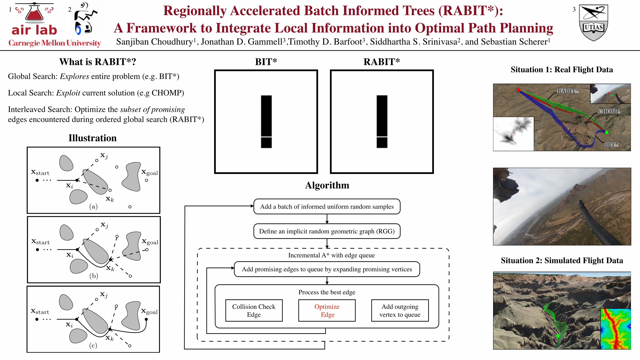
air labRegionally Accelerated Batch Informed Trees (RABIT*):
A Framework to Integrate Local Information into Optimal Path Planning Sanjiban Choudhury1, Jonathan D. Gammell3,Timothy D. Barfoot3, Siddhartha S. Srinivasa2, and Sebastian Scherer1
1 2 3
(a) (b) (c)
x
goal
x
start
xk
x
goal
x
start
x
goal
x
start
xi xi
xj
xi
xj xj
xkxk
(a) (b) (c)
x
goal
x
start
xk
x
goal
x
start
x
goal
x
start
xi xi
xj
xi
xj xj
xkxk
(a) (b) (c)
x
goal
x
start
xk
x
goal
x
start
x
goal
x
start
xi xi
xj
xi
xj xj
xkxk
Illustration
Situation 1: Real Flight DataBIT* RABIT*
RABIT*
CHOMP
BIT*
Situation 2: Simulated Flight Data
Algorithm
Add a batch of informed uniform random samples
Define an implicit random geometric graph (RGG)
Incremental A* with edge queue
Add promising edges to queue by expanding promising vertices
Process the best edge
Collision Check Edge
Optimize Edge
Add outgoing vertex to queue
What is RABIT*?
Interleaved Search: Optimize the subset of promising edges encountered during ordered global search (RABIT*)
Global Search: Explores entire problem (e.g. BIT*)
Local Search: Exploit current solution (e.g CHOMP)
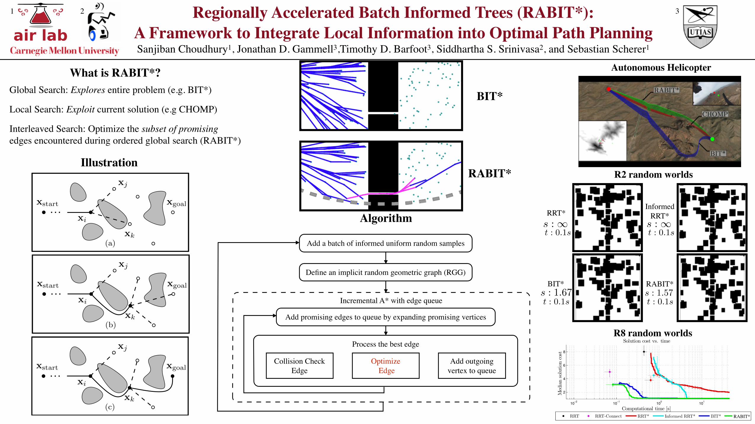
air labRegionally Accelerated Batch Informed Trees (RABIT*):
A Framework to Integrate Local Information into Optimal Path Planning Sanjiban Choudhury1, Jonathan D. Gammell3,Timothy D. Barfoot3, Siddhartha S. Srinivasa2, and Sebastian Scherer1
1 2 3
(a) (b) (c)
x
goal
x
start
xk
x
goal
x
start
x
goal
x
start
xi xi
xj
xi
xj xj
xkxk
(a) (b) (c)
x
goal
x
start
xk
x
goal
x
start
x
goal
x
start
xi xi
xj
xi
xj xj
xkxk
(a) (b) (c)
x
goal
x
start
xk
x
goal
x
start
x
goal
x
start
xi xi
xj
xi
xj xj
xkxk
Algorithm
Add a batch of informed uniform random samples
Define an implicit random geometric graph (RGG)
Incremental A* with edge queue
Add promising edges to queue by expanding promising vertices
Process the best edge
Collision Check Edge
Optimize Edge
Add outgoing vertex to queue
What is RABIT*?
Interleaved Search: Optimize the subset of promising edges encountered during ordered global search (RABIT*)
Global Search: Explores entire problem (e.g. BIT*)
Local Search: Exploit current solution (e.g CHOMP)
Illustration
10−2
10−1
100
101
2
4
6
8
Computational time [s]
Solution cost vs. time
Med
ian
solu
tion
cost
RRT RRT-Connect RRT* Informed RRT* BIT* LOB*RABIT*
R8 random worlds
InformedRRT*RRT*
s : 1 s : 1
RABIT*s : 1.57
BIT*
R2 random worlds
t : 0.1s t : 0.1s
t : 0.1s t : 0.1ss : 1.67
Autonomous Helicopter
Regionally Accelerated Batch Informed Trees (RABIT*): A Frameworkto Integrate Local Information into Optimal Path Planning
Sanjiban Choudhury1, Jonathan D. Gammell2,Timothy D. Barfoot2, Siddhartha S. Srinivasa1, and Sebastian Scherer1
Abstract— Sampling-based optimal planners, such as RRT*,almost-surely converge asymptotically to the optimal solution,but have provably slow convergence rates in high dimensions.This is because their commitment to finding the global optimumcompels them to prioritize exploration of the entire problemdomain even as its size grows exponentially. Optimizationtechniques, such as CHOMP, have fast convergence on theseproblems but only to local optima. This is because they areexploitative, prioritizing the immediate improvement of a patheven though this may not find the global optimum of nonconvexcost functions.
In this paper, we present a hybrid technique that integratesthe benefits of both methods into a single search. A key insightis that applying local optimization to a subset of edges likely toimprove the solution avoids the prohibitive cost of optimizingevery edge in a global search. This is made possible by BatchInformed Trees (BIT*), an informed global technique thatorders its search by potential solution quality. In our algorithm,Regionally Accelerated BIT* (RABIT*), we extend BIT* byusing optimization to exploit local domain information andfind alternative connections for edges in collision and accelerate
the search. This improves search performance in problemswith difficult-to-sample homotopy classes (e.g., narrow passages)while maintaining almost-sure asymptotic convergence to theglobal optimum.
Our experiments on simulated random worlds and real datafrom an autonomous helicopter show that on certain difficultproblems, RABIT* converges 1.8 times faster than BIT*.Qualitatively, in problems with difficult-to-sample homotopyclasses, we show that RABIT* is able to efficiently transformpaths to avoid obstacles.
I. INTRODUCTION
Sampling-based planners are popular for solving themotion-planning problem in robotics and are effective ona large range of applications. Algorithms such as Proba-bilistic Roadmaps (PRM) [1], Rapidly-exploring RandomTrees (RRT) [2], and Expansive Space Trees (EST) [3] areprobabilistically complete. These algorithms find a solution,if one exists, with probability one as the number of samplesgoes to infinity.
Recent research has developed asymptotically optimalplanners, such as RRT* [4]. The solutions found by thesealgorithms converge asymptotically to the optimum, if oneexists, with probability one as the number of samples goes toinfinity (i.e., almost surely). With informed search techniques,such as Informed RRT*, this convergence can be linear in
1 S. Choudhury, S. S. Srinivasa and S. Scherer are with The RoboticsInstitute at Carnegie Mellon University, Pittsburgh, Pennsylvania, USA.Email: {sanjibac, basti, siddh}@cs.cmu.edu
2 J. D. Gammell and T. D. Barfoot are with the Autonomous SpaceRobotics Lab at the University of Toronto, Toronto, Ontario, Canada. Email:{jon.gammell, tim.barfoot}@utoronto.ca
s = 1.87 s = 1.66
(a) (b)
BIT* RABIT*
Fig. 1. Solutions found by BIT* and RABIT* after 0.1 seconds ofcomputation time on a simulated 2-dimensional world. The world has anobstacle with a narrow gap that creates three homotopy classes, two ofwhich flank the obstacle and one that passes through the narrow gap. BIT*’sability to find a path through the narrow gap depends on the distributionof the random samples. RABIT* judiciously applies a local optimizer topotential edges (shown in magenta), allowing it to exploit additional probleminformation and find paths through difficult-to-sample homotopy classes(e.g., narrow passages) faster than sampling alone.
the absence of obstacles [5], but generally convergence isprovably poor, especially in high dimensions [6]. This isbecause the algorithms prioritize exploring the domain despiteits exponential growth in size with increased state dimension.
Local optimizers, such as Covariant Hamiltonian Optimiza-tion for Motion Planning (CHOMP) [7], instead prioritizeexploiting domain information, such as cost gradients, tomodify and improve a path. This rapidly finds high-qualitysolutions in high-dimensional planning problems, but onlyprovides guarantees on local optimality. This is becausenonconvex cost functions have local optima that can entrapgreedy optimization methods, such as gradient descent. Thismakes the relative suitability of local optimizers and globalsearches dependent on the specific planning problem [8].
In the field of nonconvex optimization, it is common toavoid these limitations by combining local optimization with aglobal search [9]–[14]. This provides the rapid convergence oflocal optimizers (e.g., gradient descent) with the insensitivityto local optima of a global search (e.g., stochastic search).
In this paper, we use this existing work as motivation fora framework to integrate local and global planning methodsinto a hybrid search. We do so by using Batch InformedTrees (BIT*) [15], a global method that uses heuristics tosearch in order of potential solution quality. This provides theefficiency necessary for a local optimizer to generate potentialedges from domain information (e.g., cost gradients). This
BIT*
RABIT*