1

Institut de Recerca en Economia Aplicada Regional i Pública

Research Institute of Applied Economics

Document de Treball 2017/01, 26 pàg.

Working Paper 2017/01, 26 pag.

Grup de Recerca Anàlisi Quantitativa Regional

Regional Quantitative Analysis Research Group

Document de Treball 2017/01, 26 pàg.

Working Paper 2017/01, 26 pag.

“Regional tourism demand forecasting with machine learning models: Gaussian process regression vs. neural network models in a multiple-input multiple-output setting”

Oscar Claveria, Enric Monte, Salvador Torra

Research Institute of Applied Economics Regional Quantitative Analysis Research Group

Working Paper 2017/01 Working Paper 2017/01

WEBSITE: www.ub-irea.com • CONTACT: irea@ub.edu

Universitat de Barcelona Av. Diagonal, 690 • 08034 Barcelona

The Research Institute of Applied Economics (IREA) in Barcelona was founded in 2005, as

a research institute in applied economics. Three consolidated research groups make up the

institute: AQR, RISK and GiM, and a large number of members are involved in the Institute.

IREA focuses on four priority lines of investigation: (i) the quantitative study of regional and

urban economic activity and analysis of regional and local economic policies,

(ii) study of public economic activity in markets, particularly in the fields of empirical

evaluation of privatization, the regulation and competition in the markets of public services

using state of industrial economy, (iii) risk analysis in finance and insurance, and (iv) the

development of micro and macro econometrics applied for the analysis of economic activity,

particularly for quantitative evaluation of public policies.

IREA Working Papers often represent preliminary work and are circulated to encourage

discussion. Citation of such a paper should account for its provisional character. For that

reason, IREA Working Papers may not be reproduced or distributed without the written

consent of the author. A revised version may be available directly from the author.

Any opinions expressed here are those of the author(s) and not those of IREA. Research

published in this series may include views on policy, but the institute itself takes no

institutional policy positions.

WEBSITE: www.ub.edu/aqr/ • CONTACT: aqr@ub.edu

Research Institute of Applied Economics Regional Quantitative Analysis Research Group

Working Paper 2017/01, pàg. 3Working Paper 2017/01, pag. 3

3

Abstract

This study presents a multiple-input multiple-output (MIMO) approach for

multi-step-ahead time series prediction with a Gaussian process regression

(GPR) model. We assess the forecasting performance of the GPR model with

respect to several neural network architectures. The MIMO setting allows

modelling the cross-correlations between all regions simultaneously. We find

that the radial basis function (RBF) network outperforms the GPR model,

especially for long-term forecast horizons. As the memory of the models

increases, the forecasting performance of the GPR improves, suggesting the

convenience of designing a model selection criteria in order to estimate the

optimal number of lags used for concatenation.

Keywords: Regional forecasting, tourism demand, multiple-input multiple-output

(MIMO), Gaussian process regression, neural networks, machine learning

Oscar Claveria: AQR Research Group-IREA. University of Barcelona, Av. Diagonal 690, 08034 Barcelona, Spain. E-mail: oclaveria@ub.edu Enric Monte:Department of Signal Theory and Communications, Polytechnic University of Catalunya (UPC) Salvador Torra: Riskcenter-IREA, University of Barcelona, Av. Diagonal 690, 08034 Barcelona, Spain.

4

1 Introduction

Machine learning (ML) methods are being increasingly used for economic and financial

forecasting (Ortega and Khashanah, 2014; Von Spreckelsen et al., 2014; Stasinakis et

al., 2014; Kock and Teräsvirta, 2014; Aminian et al., 2006; Medeiros et al., 2006; Chen

and Leung, 2005). International tourism is becoming one of the most important

economic activities worldwide, and as result there is an increasing interest in the

refinement of tourism demand forecasts. A growing body of literature finds evidence in

favour of a better predictive performance of machine learning models with respect to

traditional forecasting methods (Adya and Collopy, 1998; Cho, 2003; Xu et al., 2016).

Statistical learning is based on the construction of computer algorithms that learn

through experience. The complex nature of the data generating process of tourism

demand explains the increasing use of non-linear approaches such as support vector

regression (SVR) and neural network (NN) models for tourism forecasting. Akin

(2015), Chen and Wang (2007), Claveria et al. (2016b) and Hong et al. (2011) all find

that SVR models outperform linear models for tourism demand forecasting.

With respect to NN models, the most widely used NN feed-forward topology in

tourism has been the multi-layer perceptron (MLP) network (Pattie and Snyder, 1996;

Uysal and El Roubi, 1999; Law, 2000; Tsaur et al., 2002; Palmer et al., 2006; Padhi and

Aggarwal, 2011; Lin et al., 2011; Teixeira and Fernandes, 2012; Claveria et al., 2015b;

Molinet et al., 2015). See Athanasopoulos et al. (2011) and Song and Li (2008) for a

thorough review of recent tourism demand forecasting studies.

The Radial Basis Function (RBF) network, is being increasingly used for tourism

forecasting. Kon and Turner (2005) implement a RBF NN to forecast arrivals to

Singapore. More recently, Cang (2014) combines RBF, MLP and SVR forecasts of UK

inbound tourist arrivals in non-linear models. Subsequently, Çuhadar et al. (2014) and

compare the forecasting accuracy of RBF to that of MLP networks to predict tourist

demand, finding evidence in favour of RBF NNs. A complete summary on the use of

NNs with forecasting purposes can be found in Zhang et al. (1998).

Originally devised for interpolation, the Gaussian Process Regression (GPR) model

can be regarded as a supervised learning method based on a generalized linear

regression that locally estimates forecasts by the combination of values in a kernel

(Rasmussen, 1996). Gaussian process models allow to specify Bayesian priors on the

data and the structure, and therefore the use of kernel analogue for machine for learning.

5

Another key advantage of GPs over other statistical learning techniques is that they

provide full probabilistic predictive distributions, including estimations of the

uncertainty of the predictions. These features make GPR an ideal tool for forecasting

purposes (Banerjee et al., 2008; Ahmed et al., 2010; Yang et al., 2013).

In spite of the fact that GPs are powerful, non-parametric tools for regression in high

dimensional spaces, there is only one previous study that uses GPR for tourism

forecasting (Wu et al., 2012). The authors use a sparse GPR model to predict tourism

demand to Hong Kong and find that its forecasting capability outperforms those of the

ARMA and SVR models. For a unifying description of sparse approximations for GPR

see Quiñonero-Candela and Rasmussen (2005).

In order to fill this gap, we propose a multiple-output GPR model for multi-step-

ahead time series prediction. Recently, Ben Taieb et al. (2010) presented a multiple-

input multiple-output (MIMO) extension of conventional local modelling approaches

that allows to preserve the stochastic properties of the training series in multiple-step-

ahead prediction. The main aim of this study is to design a MIMO framework for multi-

step-ahead time series prediction with a GPR model.

To assess the forecasting performance of the presented GPR model we compare it to

a RBF NN and a MLP NN used as benchmark in a MIMO setting that incorporates the

cross-correlations between the inputs (international tourist arrivals to all seventeen

regions of Spain) in order to generate a vector of future values (for all markets).

The study is organized as follows. The next section reviews the literature and

describes the data. The third section presents the different machine learning methods

applied in the study. Section four describes the experimental settings and reports the

results of the multiple-step-ahead forecasting comparison. The paper concludes with

some final remarks and potential lines for future research.

2 Background and data

As a result of the growing importance of tourism as a key driver of socio-economic

progress, there is an increasing amount of literature about the contribution of tourism to

economic growth (Sánchez et al., 2015; Pérez-Rodríguez et al., 2015; Chou, 2013;

Schubert et al., 2011; Biagi and Pulina, 2009; Durbarry, 2004; Balaguer and Cantavella-

Jordá, 2002). At regional level, Paci and Marrocu (2013) evaluated the impact tourism

on economic growth in 179 European regions. By means of a spatial growth regression

6

framework, the authors found that regional growth was positively affected by domestic

and international tourism.

Most of the research on tourism at regional level in Spain focuses on three regions:

Andalusia, and the Balearic and the Canary Islands. Regarding the region of Andalusia,

Andrades-Caldito et al. (2013) analysed the destination image perceived by visitors over

the past decade. The authors quantified the degree of convergence of each province’s

tourism image relative to the overall tourism image of Andalusia as a destination, and

ranked the provinces according to their level of attractiveness as perceived by tourists,

finding a decline in the valuation of the region’s main coastal destinations in favour of

those specializing in nature and culture. Similar results were obtained by Sarrión-

Gavilán et al. (2015), who used exploratory spatial data analysis techniques to analyse

the impacts of tourism flows. In spite of a high degree of concentration in the littoral,

the authors found a more equitable territorial distribution of tourism in coastal mature

destinations and an increasing dynamism in the rural inland areas.

Bardolet and Sheldon (2008) undertook a comparative analysis between the Balearic

Islands and the Hawaiian Islands, evaluating their growth paths since the 1950s, and

identifying their strengths and weaknesses as archipelago destinations. While Capó et

al. (2007) showed that that the continuous orientation towards tourism activities had

translated in significant growth in the level of income in both the Balearic and the

Canary Islands, Vera and Ivars (2009) found evidence that the impact of low-cost

carriers in Spain had reinforced the specialization of tourism in real estate along the

Spanish Mediterranean coast.

Aguiló et al. (2005) identified the sensitivity of the tourist market in the Balearic

Islands to price changes in travel-related services. Garín-Muñoz and Montero-Marín

(2007) used a dynamic model with panel data to identify and measure the impact of the

main determinants of the inbound international tourism flows to the Balearic Islands

from the most important source markets. The authors found that consumer loyalty to the

destination was an important determinant of tourism demand. The results suggested that

the demand was heavily dependent on the evolution of economic activity in each of the

origin countries and on the relative cost of living of tourists in the destination.

By means of regression analysis, Rosselló et al. (2004) provided evidence of the

influence of economic variables on the seasonal distribution of tourist arrivals to the

Balearic Islands. The temporal concentration of tourism demand was also analysed by

Duro and Farré (2015), who found significant differences across the Spanish provinces

7

for the period 1999-2012. On one end, the Balearic and the Catalonian coastal provinces

(with the exception of Barcelona) presented the strongest seasonal pattern, while on the

other end, the Canary Islands and Madrid were the regions that showed the lowest level

of seasonality. In this sense, Priego et al. (2015) used a gravity model to show that climate

was an important factor in determining domestic tourism flows in Spain at regional level.

In the Canary Islands, Santana-Jiménez and Hernández (2011) used panel data

analysis to evaluate the influence of the tourist’s perception of overcrowding in five

islands of the archipelago, obtaining an indicator of each island’s maximum capacity.

Focusing on the island of Tenerife, Ledesma-Rodríguez et al. (2001) estimated short-run

and long-run elasticities for tourists visiting the island, obtaining significant elasticities

for income, exchange rate, cost of the trip, and infrastructure. See Aguiló (2010) for an

overview of tourism economics research in Spain from 2000 to 2010.

Despite the fact that most forecasting studies are conducted at the national level,

several regional studies have been published in recent years. Lehmann and Wohlrabe

(2015) reviewed some of the main issues related to regional forecasting. Guizzardi and

Stacchini (2015) made use of business sentiment indicators form tendency surveys for

real-time forecasting of hotel arrivals at a regional level, improving the forecasting

accuracy of structural time series models. Rickman et al. (2009) applied a A Bayesian

vector autoregression (BVAR) approach to assess whether prior information on spatial

and economic linkages improved forecast accuracy of employment for the metropolitan

areas of the state of Oklahoma and their proximate metropolitan areas.

Studies on tourism demand forecasting at regional level in Spain are mostly

concentrated in the Balearic and the Canary Islands. Regarding the Canary Islands, Gil-

Alana (2010) analysed the degree of persistence of monthly arrivals using different

time-series approaches. Gil-Alana et al. (2008) applied seasonal unit roots and

seasonally fractionally integrated models to forecast tourist arrivals to the Canary

Islands, and found that simple deterministic models with seasonal dummy variables and

AR(1) disturbances produced better results over short horizons.

For the Balearic Islands, Rosselló-Nadal (2001) predicted turning points in

international visitor arrivals from the two major source markets using the leading

indicator approach. Álvarez-Díaz and Rosselló-Nadal (2010) incorporated

meteorological variables to forecast British tourist arrivals to the Balearic Islands. More

recently, Saenz-de-Miera and Rosselló (2014) modelled tourism impacts on air

pollution in Mallorca. The authors showed that the inclusion of daily stock of tourists

8

improved the standard specification of urban air pollution models. By means of a

Generalized Additive Model they found that a 1% increase in tourists could be related to

up to a 0.45% increase in 10PM concentration levels.

The complex data generating process of tourism demand explains the increasing use

of new non-linear approaches for tourism modelling. As a result, ML methods are

experiencing a growing use in tourism forecasting (Peng et al., 2014). SVR and NN

models are the most commonly used ML techniques for tourism demand prediction.

Regarding SVR models, Chen and Wang (2007) predicted tourist arrivals to China with

SVR, back propagation NN and ARIMA models, obtaining the best forecasting results

with SVRs. Hong et al. (2011) also obtained more accurate forecasts with SVRs than

with ARIMA models for Barbados. Akin (2015) compared the forecasting results of

SVR to that of SARIMA and NN models to predict international tourist arrivals to

Turkey, obtaining the best predictions with SVR models when the slope feature is more

prominent.

There is also wide evidence in favour of NN models when compared to traditional

time series models for tourism demand forecasting (Cho, 2003; Law, 2000). The first

study that implemented ML techniques for tourism demand forecasting in Spain was

that of Palmer et al. (2006). The authors designed a MLP NN to forecast tourism

expenditure in the Balearic Islands, finding that the proposed network architecture

provided more accurate forecasts when data had been detrended and deseasonalized.

This result coincides with that of Claveria et al. (2017) for Catalonia, who analysed the

effects of data pre-processing on the forecasting performance of NN models and found

that the predictive accuracy of the models improved with seasonal adjusted data.

Medeiros et al. (2008) developed an alternative approach to analyse the demand for

international tourism in the Balearic Islands. By using a NN model that incorporated

time-varying conditional volatility and daily air passenger arrivals to Palma de

Mallorca, Ibiza and Mahon as a proxy for international tourism demand for the Balearic

Islands, the authors found that time-varying variances provided useful information

regarding the risks associated with variations in international tourist arrivals.

Whilst NN models have been widely used in economic modelling and forecasting,

other ML techniques such as GPR have been barely applied for forecasting purposes.

From a wide range of ML methods, Ahmed et al. (2010) found that an MLP NN and the

GPR showed the best forecasting performance on the monthly M3 time series

competition data. In a similar exercise, Andrawis et al. (2011) found evidence in favour

9

of a simple average combination of NN, GPR and linear models for the NN5

competition. Chapados and Bengio (2007) obtained accurate predictions of commodity

spread prices by means of GPR.

GPR models can be regarded as supervised learning methods based on a generalized

linear regression that locally estimates forecasts by the combination of values in a

kernel (Rasmussen, 1996). The works of Smola and Barlett (2001), MacKay (2003), and

Rasmussen and Williams (2006) have been key in the development of GPR models. By

expressing the model in a Bayesian framework, the authors extended GPR applications

beyond spatial interpolation to regression problems. Additional refinements have been

proposed by Belhouari and Bermak (2004) and Girard et al. (2003) who respectively

proposed using a non-stationary covariance function and the knowledge of the variance

on inputs in order to improve the forecasting performance of the GPR model. However,

up until now applications of GPR have been mostly restricted to a single-input single-

output framework.

In this study, we attempt to cover this deficit by applying an extension of the GPR

model for MIMO modelling, and assessing its forecasting performance at the regional

level. We make use of international tourist arrivals to all seventeen regions of Spain.

The MIMO GPR allows modelling the connections in tourism demand to all regions and

generate a vectorial forecast. This strategy is cost-effective in computational terms, and

seems particularly indicated for regional forecasting.

With this aim we use monthly data on international tourism demand used in this

study are collected from the Spanish Statistical Office (National Statistics Institute –

INE – www.ine.es). Our data set for the empirical experiment covers 183 monthly

observations of of tourist arrivals at a regional level from 1999:01 to 2014:03. In spite

of the fact that the forecasting performance of NNs improves when using

deseasonalized data (Nelson et al., 1999), we use the raw data in order to analyse the

forecasting accuracy of the models without using any pre-processing. In Figure 1 we

present the mean annual growth rates of the different regions. The regions marked in

grey experience a rate of growth above the average (3.7%). These regions are located in

coastal areas of the Mediterranean, showing the asymmetric concentration of tourism is

Spain (Sarrión-Gavilán et al., 2015).

10

Fig 1. Mean annual growth rate of tourist arrivals to Spain by region (1999-2013)

3 Machine learning methods

3.1 Gaussian Process Regression (GPR)

GPR was first developed by Matheron (1973) based on the geostatistic works of Krige

(1951). The works of MacKay (2003) and Rasmussen and Williams (2006) have been

crucial in the development of GPR, which can be conceived as a method of

interpolation for which the interpolated values are modelled by a GP governed by prior

covariances.

By expressing the model in a Bayesian framework, different statistical methods can

be implemented in GP models. Therefore GPR applications can be extended beyond

spatial interpolation to regression problems. GPR is used to estimate the weights of

observed values form temporal lags and spatial points using the known covariance

structures. Detailed information about GPR can be found in Rasmussen and Williams

(2006).

The GPR model assumes that the inputs ix have a joint multivariate Gaussian

distribution characterized by an analytical model of the structure of the covariance

matrix (Rasmussen, 1996). The key point of the GPR is the possibility of specifying the

functional form of the covariance functions, which allows to introduce prior knowledge

11

about the problem into the model. The training set nn yxyxyx ,,,,,, 2211 D is

assumed to be drawn from the (noisy) process:

εxfy ii with 2,0~ N (1)

where ix is an input vector in dR and iy is a scalar output in 1R . Therefore we have a

1RRd mapping. For notational convenience, we aggregate the inputs and the outputs

into matrix nxxx ,,, 21 X and nyyy ,,, 21 y respectively.

The joint distribution of the variables is the conditional Gaussian distribution:

IXX,~X2,0 KNyp (2)

where I is the identity matrix, and the covariance matrix XX,K is also called the

kernel matrix with elements jiij xxK , . The kernel function xxk , is a measure of the

distance between input vectors.

For the kernel function, a common choice is the Gaussian, or squared exponential.

In this study we make use of a radial basis kernel with a linear trend to account for the

trend component present in most of the time series over the training period:

j

T

i

ji

T

ji

jiij xxxxxx

xxkK2

2

2exp, (3)

where 2υ controls the prior variance, and λ is a parameter that controls the rate of

decay of the covariance by determining how far away ix must be from jx for if to be

unrelated to jf . Alternative sets of kernels are discussed in MacKay (2003). The

hyperparameters κγλυ ,,, are estimated by maximum likelihood in:

2log2

log2

1

2

1log 212 n

yyxyp T

IXX,KIXX,K (4)

Given the training samples ji yx , and a set of test points *X , the objective of

GPR is to find the predictive outputs *f with probabilistic confidence intervals. By

making use of the Bayesian inference, the joint posterior distribution is:

Xyp

ffpfypyffp

** ,

, (5)

The joint prior distribution and the independent likelihood probability both follow a

Gaussian distribution:

**,*,

*,,* ,0,

ffff

ffff

KK

KK

Nffp (6)

12

IσfNfyp 2, (7)

where f and *f are subscripts of the variables between which the covariance is

computed. The Gaussian predictive distribution yfp * is characterized by mean μ

and variance .

Therefore the GPR model specification is given by equations:

yIXXK12*,

XX,K (8)

*,*,**,12 XXKIXXKXXK

XX,K (9)

where μ is the predicted output, and the variance can be used to estimate confidence

levels.

In this study we propose an extension of the model to multiple outputs based on an

analogy to radial basis functions. We use a set of univariate predictors followed by a

matrix product that takes into account the cross-dependencies of the outputs in order to

improve the performance of the GPR. In this case we have a Md RR , where M is

the dimension of the output. This extension is applied by following a two-step training.

First, we independently train each time series, generating supervised forecasts for each

output. In the second step, by means of a regularized linear regression (Haykin, 2008),

we generate forecasts for each output taking into account their correlations. This

procedure is also applied to the NN models.

3.2 Neural Network models

3.2.1 Radial Basis Function (RBF)

Initially proposed by Broomhead and Lowe (1988), RBF networks are hybrid networks

that combine both supervised and non-supervised learning. RBF NN are a special class

of multi-layer feed-forward architecture with several layers of processing. First, an input

layer, modelled as a feature vector of real numbers. Second, a hidden layer, which

consists of a set of neurons, each of them computing a symmetric radial function

centred each at a centroid j . Finally, an output layer that consists of a set of neurons,

one for each given output. The output of the network can be expressed as a scalar

function of the output vector of the hidden layer:

13

qj

pix

x

xg

xgy

j

it

j

p

jjit

itj

itjj

q

jt

,,1 ; ;

,,1 ;

2exp

j

2

1

2

10

(10)

where ty is the output vector of the network at time t ; itx is the input value at time

it , where i stands for the number of lags that are used to introduce the context of the

actual observation; jg is the activation function, which usually has a Gaussian shape;

j are the weights connecting the output of the neuron j at the hidden layer with the

output neuron; j is the centroid vector for neuron j ; and the spread j is a scalar

that measures the width over the input space of the Gaussian function. We denote q as

the number of neurons in the hidden layer, which ranges from 5 to 30, increasing for

longer forecasting horizons.

3.2.2 Multi-layer Perceptron (MLP)

MLP networks consist of multiple layers of computational units interconnected in a

feed-forward way. MLP networks are supervised neural networks that use as a building

block a simple perceptron model. The topology consists of layers of parallel

perceptrons, with optimal connections between layers:

qj

qjpiw

pix

wxwgy

j

ij

it

j

p

iitijj

q

jt

,,1;

,,1,,1;

,,1;

011

0

;

(11)

where ty is the output vector of the network at time t ; itx is the input value at time

it ; j are the weights connecting the output of the neuron j at the hidden layer with

the output neuron;. ijw stand for the weights of neuron j connecting the input with the

hidden layer; and g is the non-linear function of the neurons in the hidden layer. The

number of neurons in the hidden layer is denoted by q , and determines the network’s

capacity to approximate a given function. In order to solve the problem of overfitting,

the number of neurons is estimated by cross-validation.

14

4 Forecasting comparison

4.1 Experimental design

For an iterated multi-step-ahead forecasting comparison the partition between train

and test sets is done sequentially: as the prediction advances, past forecasts are

successively incorporated to the training database. As the size of the training set

increases, for each predicted value in the test database, the first element of the validation

database is transferred to the training database, and the last predicted value of the test

database is incorporated to the validation database in a recursive way. Thus, the first

ninety-six monthly observations are selected as the initial training set, the next 33% as

the validation set, and the last 15% as the test set.

Once the topology of the neural networks is decided, the parameters of the networks

are estimated by means of the Levenberg-Marquardt (LM) algorithm. In order to assure

a correct performance of the RBF NNs, the number of centroids and the spread of each

centroid have to be selected before the training phase. In this study the training is done

by adding the centroids iteratively with the spread parameter fixed. Then a regularized

linear regression is estimated to compute the connections between the hidden and the

output layer. Finally, the performance of the networks is computed on the validation

data set. This process is repeated until the performance on the validation database ceases

to decrease. To avoid the possibility that the search for the optimum value of the

parameters finishes in a local minimum, we use a multi-starting technique that

initializes the NNs several times for different initial random values and returns the best

result. All models are implemented with Python.

4.2 Experimental results

To assess the performance of the GPR model, we compare its forecasting accuracy to

that of a RBF NN. We estimate the models and generate forecasts in a recursive way for

different forecast horizons (1, 3, 6 and 12 months) during the out-of-sample period. In

order to summarize the results of the forecasting comparison, we compute several

forecast accuracy measures. First we obtain the Relative Mean Absolute Percentage

Error (rMAPE) statistic for the GPR and the RBF NN with respect to a MLP NN model

15

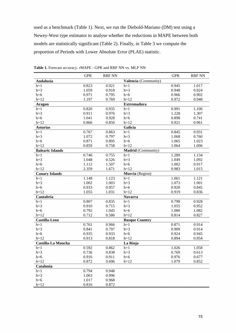
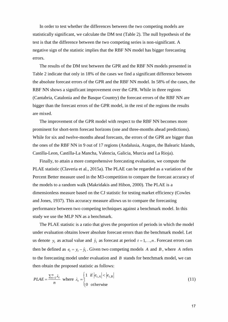
used as a benchmark (Table 1). Next, we run the Diebold-Mariano (DM) test using a

Newey-West type estimator to analyse whether the reductions in MAPE between both

models are statistically significant (Table 2). Finally, in Table 3 we compute the

proportion of Periods with Lower Absolute Error (PLAE) statistic.

Table 1. Forecast accuracy. rMAPE - GPR and RBF NN vs. MLP NN

GPR RBF NN GPR RBF NN

Andalusia Valencia (Community)

h=1 0.823 0.921 h=1 0.945 1.017

h=3 1.059 0.918 h=3 0.948 0.924

h=6 0.971 0.795 h=6 0.966 0.902

h=12 1.197 0.769 h=12 0.972 0.948

Aragon Extremadura

h=1 0.820 0.935 h=1 0.991 1.106

h=3 0.911 0.976 h=3 1.228 1.307

h=6 1.041 0.928 h=6 0.898 0.741

h=12 0.866 0.850 h=12 0.921 0.961

Asturias Galicia

h=1 0.767 0.863 h=1 0.845 0.931

h=3 1.072 0.797 h=3 1.068 0.760

h=6 0.871 0.895 h=6 1.065 1.023

h=12 0.859 0.758 h=12 1.064 1.006

Balearic Islands Madrid (Community)

h=1 0.746 0.755 h=1 1.289 1.134

h=3 1.048 0.526 h=3 1.049 1.092

h=6 1.112 1.507 h=6 1.002 0.917

h=12 2.359 1.671 h=12 0.983 1.015

Canary Islands Murcia (Region)

h=1 1.148 1.123 h=1 1.061 1.121

h=3 1.002 1.003 h=3 1.073 1.001

h=6 0.933 0.957 h=6 0.920 0.845

h=12 1.055 1.031 h=12 0.919 0.836

Cantabria Navarra

h=1 0.807 0.835 h=1 0.798 0.928

h=3 0.910 0.715 h=3 1.055 0.952

h=6 0.792 1.045 h=6 1.080 1.082

h=12 0.712 0.586 h=12 0.814 0.827

Castilla-Leon Basque Country

h=1 0.761 0.966 h=1 0.871 0.914

h=3 0.841 0.797 h=3 0.909 0.914

h=6 0.935 0.933 h=6 0.924 0.945

h=12 0.913 0.818 h=12 0.894 0.954

Castilla-La Mancha La Rioja

h=1 0.592 0.862 h=1 1.026 1.058

h=3 0.736 0.838 h=3 0.769 0.613

h=6 0.916 0.911 h=6 0.976 0.677

h=12 0.872 0.696 h=12 1.079 0.852

Catalonia

h=1 0.794 0.948

h=3 1.063 0.996

h=6 1.017 0.968

h=12 0.816 0.872

16

Table 2. DM test statistic - GPR vs. RBF NN

Andalusia Valencia (Community)

h=1 -2.384 h=1 -1.941

h=3 0.309 h=3 -0.207

h=6 1.619 h=6 1.784

h=12 6.426 h=12 1.138

Aragon Extremadura

h=1 -1.776 h=1 -1.755

h=3 -1.455 h=3 -1.702

h=6 2.766 h=6 1.747

h=12 0.632 h=12 -1.090

Asturias Galicia

h=1 -1.846 h=1 -2.733

h=3 0.884 h=3 0.864

h=6 -0.218 h=6 0.666

h=12 1.670 h=12 0.594

Balearic Islands Madrid (Community)

h=1 -1.941 h=1 2.334

h=3 0.668 h=3 -1.258

h=6 1.161 h=6 1.449

h=12 0.973 h=12 -0.269

Canary Islands Murcia (Region)

h=1 0.485 h=1 -0.214

h=3 -0.226 h=3 -0.029

h=6 -1.208 h=6 1.169

h=12 0.494 h=12 1.586

Cantabria Navarra

h=1 -0.437 h=1 -1.300

h=3 0.256 h=3 0.852

h=6 -0.051 h=6 -1.267

h=12 -0.460 h=12 0.788

Castilla-Leon Basque Country

h=1 -6.729 h=1 -1.626

h=3 -0.557 h=3 -0.960

h=6 1.283 h=6 -0.748

h=12 3.338 h=12 -0.899

Castilla-La Mancha La Rioja

h=1 -2.848 h=1 -0.459

h=3 -1.792 h=3 -0.325

h=6 0.660 h=6 3.425

h=12 2.325 h=12 2.616

Catalonia

h=1 -3.758

h=3 -0.242

h=6 1.714

h=12 -0.027

Note: The 5% level critical value is 2.028

The results of the rMAPE for the GPR and the RBF NN models presented in Table

1 show that there are no major differences between both models when compared to a

MLP NN. By regions, in the Balearic Islands, Madrid and the Canary Islands the MLP

NN is rarely outperformed. In contrast, in Cantabria, Castilla-Leon, Castilla-La Mancha,

and the Basque Country, both the GPR model and the RBF NN outperform the MLP for

all forecast horizons.

17

In order to test whether the differences between the two competing models are

statistically significant, we calculate the DM test (Table 2). The null hypothesis of the

test is that the difference between the two competing series is non-significant. A

negative sign of the statistic implies that the RBF NN model has bigger forecasting

errors.

The results of the DM test between the GPR and the RBF NN models presented in

Table 2 indicate that only in 18% of the cases we find a significant difference between

the absolute forecast errors of the GPR and the RBF NN model. In 58% of the cases, the

RBF NN shows a significant improvement over the GPR. While in three regions

(Cantabria, Catalonia and the Basque Country) the forecast errors of the RBF NN are

bigger than the forecast errors of the GPR model, in the rest of the regions the results

are mixed.

The improvement of the GPR model with respect to the RBF NN becomes more

prominent for short-term forecast horizons (one and three-months ahead predictions).

While for six and twelve-months ahead forecasts, the errors of the GPR are bigger than

the ones of the RBF NN in 9 out of 17 regions (Andalusia, Aragon, the Balearic Islands,

Castilla-Leon, Castilla-La Mancha, Valencia, Galicia, Murcia and La Rioja).

Finally, to attain a more comprehensive forecasting evaluation, we compute the

PLAE statistic (Claveria et al., 2015a). The PLAE can be regarded as a variation of the

Percent Better measure used in the M3-competition to compare the forecast accuracy of

the models to a random walk (Makridakis and Hibon, 2000). The PLAE is a

dimensionless measure based on the CJ statistic for testing market efficiency (Cowles

and Jones, 1937). This accuracy measure allows us to compare the forecasting

performance between two competing techniques against a benchmark model. In this

study we use the MLP NN as a benchmark.

The PLAE statistic is a ratio that gives the proportion of periods in which the model

under evaluation obtains lower absolute forecast errors than the benchmark model. Let

us denote ty as actual value and ty as forecast at period nt ,,1 . Forecast errors can

then be defined as ttt yye ˆ . Given two competing models A and B , where A refers

to the forecasting model under evaluation and B stands for benchmark model, we can

then obtain the proposed statistic as follows:

n

λPLAE

nt t

1 where

otherwise 0

if 1 ,, BtAt

t

eeλ (11)

18

Table 3. Forecast accuracy. PLAE - GPR and RBF NN vs. MLP NN

GPR RBF NN GPR RBF NN

Andalusia Valencia (Community) h=1 0.364 0.273 h=1 0.182 0.910

h=3 0.273 0.545 h=3 0.273 0.455

h=6 0.455 0.545 h=6 0.364 0.455

h=12 0.818 0.818 h=12 0.636 0.727

Aragon Extremadura h=1 0.273 0.273 h=1 0.182 0.182

h=3 0.545 0.727 h=3 0.273 0.727

h=6 0.727 0.545 h=6 0.727 0.818

h=12 0.636 0.727 h=12 0.909 0.818

Asturias Galicia h=1 0.182 0.182 h=1 0.910 0.910

h=3 0.545 0.909 h=3 0.636 0.818

h=6 0.818 0.818 h=6 0.818 0.909

h=12 0.818 0.818 h=12 0.909 0.909

Balearic Islands Madrid (Community) .

h=1 0.545 0.545 h=1 0.000 0.182

h=3 0.818 0.909 h=3 0.182 0.182

h=6 0.909 1.000 h=6 0.182 0.273

h=12 1.000 1.000 h=12 0.000 0.000

Canary Islands Murcia (Region)

h=1 0.000 0.000 h=1 0.910 0.182

h=3 0.000 0.000 h=3 0.364 0.545

h=6 0.000 0.000 h=6 0.364 0.455

h=12 0.000 0.000 h=12 0.636 0.818

Cantabria Navarra

h=1 0.364 0.364 h=1 0.182 0.910

h=3 0.818 0.909 h=3 0.545 0.818

h=6 0.818 0.909 h=6 0.636 0.727

h=12 1.000 0.909 h=12 0.727 0.636

Castilla-Leon Basque Country

h=1 0.545 0.910 h=1 0.182 0.182

h=3 0.636 0.909 h=3 0.273 0.455

h=6 0.727 0.818 h=6 0.545 0.455

h=12 0.909 0.909 h=12 0.910 0.273

Castilla-La Mancha La Rioja

h=1 0.636 0.545 h=1 0.182 0.273

h=3 0.727 0.909 h=3 0.727 0.909

h=6 0.818 0.818 h=6 0.727 0.727

h=12 0.818 0.818 h=12 0.818 0.909

Catalonia

h=1 0.273 0.910

h=3 0.36.4 0.545

h=6 0.818 0.818

h=12 0.727 0.727

Note: The PLAE ratio measures the proportion of out-of-sample periods with lower absolute errors than the

benchmark model (MLP NN model). Values below 0.5 indicate that the benchmark model displays a higher

number of lower absolute forecast errors than the model under evaluation for the out-of-sample period.

19

Table 3 shows the results of the PLAE statistic for the GPR and the RBF NN

compared to the MLP NN. We do not find relevant differences between the GPR and

the RBF NN when compared to the MLP NN. Both the GPR and the RBF NN display

higher PLAE values than the MLP NN for all forecast horizons except for one-month

ahead predictions, where the MLP NN shows a higher proportion of out-of-sample

periods with lower absolute errors in all regions except two (the Balearic Islands and

Castilla-La Mancha). Special mention should be made to the Canary Islands and the

Community of Madrid, where neither model outperforms the MLP NN regardless of the

forecast horizon. These results are in line with those obtained in Table 1.

In order to evaluate the effect of the memory on the forecasting results, we repeat

the experiment considering different topologies regarding the number of lags used for

concatenation. In Table 4 we present the results of the rMAPE and the DM test for the

GPR model with a memory of one period with respect to the GPR with i =3. We find

that when additional lags are incorporated in the feature vector, the rMAPE results show

that the forecasting performance of the GPR models improves in almost 70% of the

cases.

Finally, in Table 4 we also present the results of the DM test between the GPR with

a one-period memory and the GPR with a three-period memory. We find that in 54% of

the cases there is a significant difference between the absolute forecasting errors of the

GPR for i =1 and the GPR for i =3. In 90% of the cases, incorporating additional lags in

the model results in a significant improvement. Madrid and the Canary Islands are the

only regions where there is no significant reduction in forecasting errors when

increasing the memory of the model. The fact that both regions are the ones with the

lowest temporal concentration of tourism demand suggests that increasing the memory

of the models is particularly indicated when the series present a marked seasonal

component. This evidence is in line with the results obtained by Claveria et al. (2016a),

who found that GPR models could not outperform naïve forecasts in the absence of

seasonality regardless of the forecast horizon.

Overall, the empirical experiment shows that the forecasting performance of the

different techniques improves for longer forecast horizons. For the Balearic Islands,

Palmer et al. (2006) found that NNs were especially suitable for long-term forecasting,

which is in line with previous research by Burger et al. (2001), Pattie and Snyder (1996)

and Teräsvirta et al. (2005). However, we find that the RBF NN generates better

predictions than the GPR models when compared to a MLP NN, especially for longer-

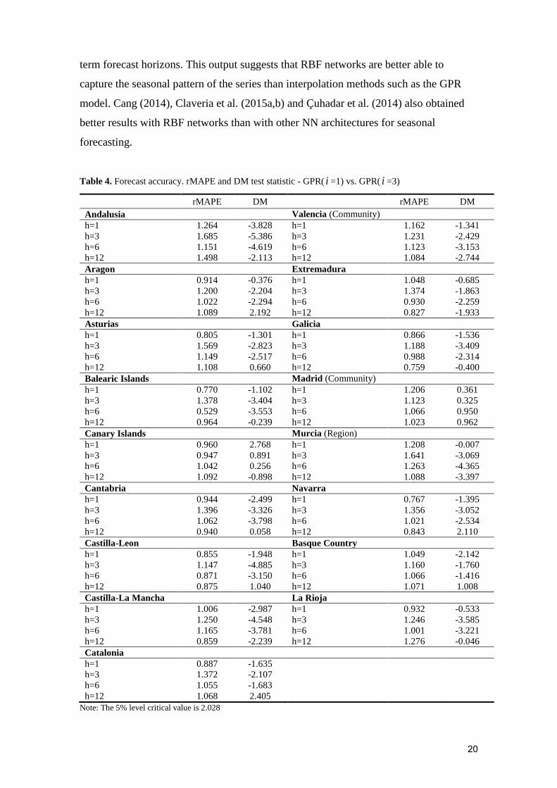
20

term forecast horizons. This output suggests that RBF networks are better able to

capture the seasonal pattern of the series than interpolation methods such as the GPR

model. Cang (2014), Claveria et al. (2015a,b) and Çuhadar et al. (2014) also obtained

better results with RBF networks than with other NN architectures for seasonal

forecasting.

Table 4. Forecast accuracy. rMAPE and DM test statistic - GPR( i =1) vs. GPR( i =3)

rMAPE DM rMAPE DM

Andalusia Valencia (Community)

h=1 1.264 -3.828 h=1 1.162 -1.341

h=3 1.685 -5.386 h=3 1.231 -2.429

h=6 1.151 -4.619 h=6 1.123 -3.153

h=12 1.498 -2.113 h=12 1.084 -2.744

Aragon Extremadura

h=1 0.914 -0.376 h=1 1.048 -0.685

h=3 1.200 -2.204 h=3 1.374 -1.863

h=6 1.022 -2.294 h=6 0.930 -2.259

h=12 1.089 2.192 h=12 0.827 -1.933

Asturias Galicia

h=1 0.805 -1.301 h=1 0.866 -1.536

h=3 1.569 -2.823 h=3 1.188 -3.409

h=6 1.149 -2.517 h=6 0.988 -2.314

h=12 1.108 0.660 h=12 0.759 -0.400

Balearic Islands Madrid (Community)

h=1 0.770 -1.102 h=1 1.206 0.361

h=3 1.378 -3.404 h=3 1.123 0.325

h=6 0.529 -3.553 h=6 1.066 0.950

h=12 0.964 -0.239 h=12 1.023 0.962

Canary Islands Murcia (Region)

h=1 0.960 2.768 h=1 1.208 -0.007

h=3 0.947 0.891 h=3 1.641 -3.069

h=6 1.042 0.256 h=6 1.263 -4.365

h=12 1.092 -0.898 h=12 1.088 -3.397

Cantabria Navarra

h=1 0.944 -2.499 h=1 0.767 -1.395

h=3 1.396 -3.326 h=3 1.356 -3.052

h=6 1.062 -3.798 h=6 1.021 -2.534

h=12 0.940 0.058 h=12 0.843 2.110

Castilla-Leon Basque Country

h=1 0.855 -1.948 h=1 1.049 -2.142

h=3 1.147 -4.885 h=3 1.160 -1.760

h=6 0.871 -3.150 h=6 1.066 -1.416

h=12 0.875 1.040 h=12 1.071 1.008

Castilla-La Mancha La Rioja

h=1 1.006 -2.987 h=1 0.932 -0.533

h=3 1.250 -4.548 h=3 1.246 -3.585

h=6 1.165 -3.781 h=6 1.001 -3.221

h=12 0.859 -2.239 h=12 1.276 -0.046

Catalonia

h=1 0.887 -1.635

h=3 1.372 -2.107

h=6 1.055 -1.683

h=12 1.068 2.405

Note: The 5% level critical value is 2.028

21

When comparing the forecasting accuracy of a sparse GPR model than with ARMA

and SVR models for tourist arrivals to Hong Kong, Wu et al. (2012) obtained better

forecasting results with the GPR model. In our case, the GPR model only outperformed

the RBF NN for short-term forecast horizons. Nevertheless, there are several differences

between both approaches. On the one hand, the models used in the forecasting

comparison differ between both studies. In this experiment we compared a GPR model

to a RBF NN architecture, using a MLP NN model as a benchmark. Moreover, we did

not apply any sparse approximation to reduce the computational complexity of the GPR

model due to the size of the sample. On the other hand, we applied a MIMO setting

instead of a single-input single-output approach. In this sense, Ben Taieb et al. (2010)

and Claveria et al. (2015a) also found evidence that MIMO strategies for ML techniques

were particularly suitable for long-term forecasting.

4 Concluding remarks

In this study we present a multiple-input multiple-output (MIMO) framework for

Gaussian process regression (GPR). In order to examine the predictive performance of

the proposed method we compare its out-of-sample forecast accuracy to that of two

neural network architectures (RBF NN and MLP NN) in a multiple-step-ahead

forecasting comparison. The MIMO forecasting strategy allows modelling the

interdependencies between the inputs in order to generate a vector of future values. By

using the cross-correlations between tourist arrivals to all seventeen regions of Spain we

forecast tourist demand for all markets simultaneously.

The forecasting results show that the proposed extension of the GPR only

outperforms the NN models for short-term forecasts. We find that the predictive

performance of all techniques improves for for the longest forecast horizons, which

suggests that machine learning techniques are specially suitable for mid and long-term

forecasting.

To evaluate the effect of an increase in the dimensionality of the input on forecast

accuracy, we repeat the experiment by increasing the temporal context. As we increase

the number of lags used for concatenation, we find that the forecasting performance of

MIMO GPR models improves. This finding shows that the increase in the weight matrix

is compensated by a more complex specification, and highlights the convenience of

22

designing a model selection criteria to estimate the optimal number of lags when

forecasting with machine learning methods.

The assessment of alternative kernel functions that can support a broader class of

covariance functions on the forecasting accuracy of GPR models is a question to be

addressed in further research. Another question to be considered in future research is the

effect of different sparse approximations for parameter estimation on forecast accuracy.

References

Adya M, Collopy F (1998) How effective are neural networks at forecasting and prediction? A

review and evaluation. Journal of Forecasting 17: 481–495.

Aguiló E (2010) Una panorámica de la economía del turismo en España. Cuadernos de

Economía 33: 5–42.

Aguiló E, Riera A, Rosselló J (2005) The short-term price effect of a tourist tax through a

dynamic demand model: The Case of the Balearic Islands. Tourism Management 26: 359–

365.

Ahmed NK, Atiya AF, El Gayar N, El-Shishiny H (2010) An empirical comparison of machine

learning models for time series forecasting. Econometric Reviews 29:594–621.

Akin M (2015) A novel approach to model selection in tourism demand modeling. Tourism

Management 48: 64–72.

Álvarez-Díaz M, Rosselló-Nadal J (2010) Forecasting British tourist arrivals in the Balearic

Islands using meteorological variables. Tourism Economics 16: 153–168.

Andrades-Caldito L, Sánchez-Rivero M, Pulido-Fernández JI (2013) Differentiating

competitiveness through tourism image assessment. An application to Andalusia (Spain).

Journal of Travel Research 52: 68–81.

Andrawis RR, Atiya AF, El-Shishiny H (2011) Forecast combinations of computational

intelligence and linear models for the NN5 time series forecasting competition.

International Journal of Forecasting 27: 672–688.

Aminian F, Dante E, Aminian M, Waltz D (2006) Forecasting economic data with neural

networks. Computational Economics 28: 71–88.

Athanasopoulos G, Hyndman RJ, Song H, Wu DC (2011) The tourism forecasting competition.

International Journal of Forecasting 27: 822–844.

Balaguer J, Cantavella-Jordá M (2002) Tourism as a long-run economic growth tactor: The

Spanish case. Applied Economics 34: 877–884.

Banerjee S, Gelfand AE, Finley AO, Sang H (2008) Gaussian predictive process models for

large spatial data sets. Journal of the Royal Statistical Society: Series B (Statistical

Methodology), 70: 825–848.

Bardolet E, Sheldon PJ (2008) Tourism in archipelagos. Hawai’i and the Balearics. Annals of

Tourism Research 35: 900–923.

Ben Taieb S, Sorjamaa A, Bontempi G (2010) Multiple-output Modeling for Multi-step-ahead

Time Series Forecasting. Neurocomputing 73: 1950–1957.

Biagi B, Pulina M (2009) Bivariate VAR models to test Granger causality between tourist

demand and supply: Implications for regional sustainable growth. Papers in Regional

Science 88: 231–244.

Brahim-Belhouari S, Bermak A (2004) Gaussian process for nonstationary time series

prediction. Computational Statistics & Data Analysis 47: 705–712.

Broomhead DS., Lowe D (1988) Multi-variable functional interpolation and adaptive networks.

Complex Syst. 2: 321–355.

23

Burger C, Dohnal M, Kathrada M, Law R (2001) A practitioners guide to time-series methods

for tourism demand forecasting: A case study of Durban, South Africa. Tourism

Management 22: 403–409.

Cang S (2014) A Comparative analysis of three types of tourism demand forecasting models:

Individual, linear combination and non-linear combination. International Journal of

Tourism Research 16: 596–607.

Capó J, Riera A, Rosselló J (2007). Tourism and long-term growth. A Spanish perspective.

Annals of Tourism Research 34: 709–726.

Chapados, N., Bengio, Y., 2007. Augmented functional time series representation and

forecasting with Gaussian processes. In B. Schölkopf, J. C. Platt, & T. Hoffman (Eds.),

Advances in Neural Information Processing Systems, 19 (pp. 457–464). The MIT Press,

Cambridge, MA.

Chen AS, Leung MT (2005) Performance evaluation of neural network architectures: The case

of predicting foreign exchange correlations. Journal of Forecasting 24: 403–420.

Chen KY, Wang CH (2007) Support vector regression with genetic algorithms in forecasting

tourism demand. Tourism Management 28: 215–226.

Cho V (2003) A comparison of three different approaches to tourist arrival forecasting. Tourism

Management 24: 323–330.

Chou MC (2013) Does tourism development promote economic growth in transition countries?

A panel data analysis. Economic Modelling 33: 226–232.

Claveria O, Torra S (2014) Forecasting tourism demand to Catalonia: Neural networks vs. time

series models. Economic Modelling 36: 220–228.

Claveria O, Monte E, Torra S (2015a) A new forecasting approach for the hospitality industry.

International Journal of Contemporary Hospitality Management 27: 1520–1538.

Claveria O, Monte E, Torra S (2015b) Tourism demand forecasting with neural network

models: Different ways of treating information. International Journal of Tourism Research

17: 492–500.

Claveria O, Monte E, Torra S (2016a) Modelling cross-dependencies between Spain’s regional

tourism markets with an extension of the Gaussian process regression model. SERIEs 7:

341–357.

Claveria O, Monte E, Torra S (2016b) Modelling tourism demand to Spain with machine

learning techniques. The impact of forecast horizon on model selection. Revista de

Economía Aplicada 24(72): 109–132.

Claveria O, Monte E, Torra S (2017) Data pre-processing for neural network-based forecasting:

Does it really matter? Technical and Economic Development of Economy. Forthcoming.

Cowles A, Jones H (1937) Some a posteriori probabilities in stock market action. Econometrica

5: 280–294.

Çuhadar M, Cogurcu I, Kukrer C (2014) Modelling and forecasting cruise tourism demand to

İzmir by different artificial neural network architectures. International Journal of Business

and Social Research 4: 12–28.

De la Mata R, Llano-Verduras E (2012) Spatial pattern and domestic tourism: An econometric

analysis using inter-regional monetary flows by type of journey. Papers in Regional

Science 91: 437–470.

Durbarry R (2004) Tourism and economic growth: the case of Mauritius. Tourism Economics

10: 389–401.

Duro JA, Farré FX (2015) Estacionalidad turística en las provincias españolas: Medición y

análisis. Cuadernos de Turismo 36: 157–174.

Garín-Muñoz T, Montero-Martín LF (2007) Tourism in the Balearic Islands: A dynamic model

for international demand using panel data. Tourism Management 28: 1224–1235.

Gil-Alana LA (2010) International arrivals in the Canary Islands: Persistence, long memory,

seasonality and other implicit dynamics. Tourism Economics 16: 287–302.

Gil-Alana LA, Cunado J, De Gracia FP (2008) Tourism in the Canary Islands: Forecasting

using several seasonal time series models. Journal of Forecasting 27: 621–636.

Girard A, Rasmussen C, Quiñonero-Candela J, Murray-Smith R (2003) Multiple-step ahead

prediction for non linear dynamic systems – a Gaussian process treatment with propagation

24

of the uncertainty. In S. Becker, S. Thrun, & K. Obermayer (Eds.), Advances in Neural

Information Processing Systems 15. The MIT Press, Cambridge, MA.

Guizzardi A, Stacchini A (2015) Real-time forecasting regional tourism with business sentiment

surveys. Tourism Management 47: 213–223.

Haykin S (2008) Neural Networks and Learning Machines. Prentice Hall, New Jersey.

Hong W, Dong Y, Chen L, Wei S (2011) SVR with hybrid chaotic genetic algorithms for

tourism demand forecasting. Applied Soft Computing 11: 1881–1890.

Kock AB, Teräsvirta T (2014) Forecasting performances of three automated modelling

techniques during the economic crisis 2007-2009. International Journal of Forecasting 30:

616–631.

Kon S, Turner LL (2005) Neural network forecasting of tourism demand. Tourism Economics

11: 301–328.

Krige DG (1951) A statistical approach to some basic mine valuation problems on the

Witwatersrand. Journal of the Chemistry, Metallurgical and Mining Society of South

Africa 52: 119–139.

Law R (2000) Back-propagation learning in improving the accuracy of neural network-based

tourism demand forecasting. Tourism Management 21: 331–340.

Ledesma-Rodríguez FJ, Navarro-Ibanez M, Pérez-Rodríguez JV (2001) Panel data and tourism:

A case study of Tenerife. Tourism Economics 7: 75–88.

Lehmann R, Wohlrabe K. 2015. Forecasting GDP at the regional level with many predictors.

German Economic Review 16: 226–254.

Lin C, Chen H, Lee T (2011) Forecasting tourism demand using time series, artificial neural

networks and multivariate adaptive regression splines: Evidence from Taiwan.

International Journal of Business Administration 2: 14–24.

MacKay DJC (2003) Information Theory, Inference, and Learning Algorithms. Cambridge

University Press: Cambridge.

Makridakis S, Hibon M (2000) The M3-competition: results, conclusions and implications.

International Journal of Forecasting 16: 451–476.

Matheron G (1973) The intrinsic random functions and their applications. Advances in Applied

Probability 5: 439–468.

Medeiros MC, Teräsvirta T, Rech G (2006) Building neural network models for time series: A

statistical approach. Journal of Forecasting 25: 49–75.

Medeiros MC, McAleer M, Slottje D, Ramos V, Rey-Maquieira J (2008) An alternative

approach to estimating demand: Neural network regression with conditional volatility for

high frequency air passenger arrivals. Journal of Econometrics 147: 372–383.

Molinet T, Molinet JA, Betancourt ME, Palmer A, Montaño JJ (2015) Models of artificial

neural networks applied to demand forecasting in nonconsolidated tourist destinations.

Methodology: European Journal of Research Methods for the Behavioral and Social

Sciences 11: 35–44.

Nelson M, Hill T, Remus W, O’Connor M (1999) Time series forecasting using neural

networks: Should the data be deseasonalized first?. Journal of Forecasting 18: 359–367.

Ortega L, Khashanah K (2014) A neuro-wavelet model for the short-term forecasting of high-

frequency time series of stock returns. Journal of Forecasting 33: 134–146.

Paci R, Marrocu E (2014) Tourism and regional growth in Europe. Papers in Regional Science

93(S1): S25–S50.

Padhi SS, Aggarwal V (2011) Competitive revenue management for fixing quota and price of

hotel commodities under uncertainty. International Journal of Hospitality Management 30:

725–734.

Palmer A, Montaño JJ, Sesé A (2006) Designing an artificial neural network for forecasting

tourism time-series. Tourism Management 27: 781-790.

Pattie DC, Snyder J (1996) Using a neural network to forecast visitor behavior. Annals of

Tourism Research 23: 151–164.

Peng B, Song H, Crouch GI (2014) A Meta-analysis of international tourism demand

forecasting and implications for practice. Tourism Management 45: 181–193.

Pérez-Rodríguez JV, Ledesma-Rodríguez F, Santana-Gallego M (2015) Testing dependence

between GDP and tourism's growth rates. Tourism Management 48: 268–282.

25

Priego FJ, Rosselló J, Santana-Gallego M (2015) The impact of climate change on domestic

tourism: a gravity model for Spain. Regional Environmental Change 15: 291–300.

Quiñonero-Candela J, Rasmussen CE (2005) A unifying view of sparse approximate Gaussian

process regression. Journal of Machine Learning Research 6: 1939–1959.

Rasmussen CE (1996) The infinite Gaussian mixture model. Advances in Neural Information

Processing Systems 8: 514–520.

Rasmussen CE, Williams CKI (2006) Gaussian Processes for Machine Learning. The MIT

Press: Cambridge, MA.

Rickman DS, Miller SR, McKenzie R (2009) Spatial and sectoral linkages in regional models:

A Bayesian vector autoregression forecast evaluation. Papers in Regional Science 88: 29–

41.

Rosselló J, Riera A, Sansó A (2004) The economic determinants of seasonal patterns. Annals of

Tourism Research 31: 697–711.

Rosselló-Nadal J (2001) Forecasting turning points in international visitor arrivals in the

Balearic Islands. Tourism Economics 7: 365–380.

Saenz-de-Miera O, Rosselló J (2014) Modeling tourism impacts on air pollution: the case study

of 10PM in Mallorca. Tourism Management 40: 273–281.

Sánchez M, Cárdenas PJ, Pulido JI (2015) Does tourism growth influence economic

development? Journal of Travel Research 54: 206–221.

Santana-Jiménez Y, Hernández JM (2011) Estimating the effect of overcrowding on tourist

attraction: The case of Canary Islands. Tourism Management 32: 415–425.

Sarrión-Gavilán MD, Benítez-Márquez MD, Mora-Rangel EO (2015) Spatial distribution of

tourism supply in Andalusia. Tourism Management 15: 29–45.

Schubert SF, Brida JG, Risso WA (2011). The impacts of international tourism demand on

economic growth of small economies dependent on tourism. Tourism Management 32:

377–385.

Smola AJ, Bartlett PL (2001) Sparse greedy Gaussian process regression. In T. K. Leen, T. G.

Dietterich, and V. Tresp (Eds.) Advances in Neural Information Processing Systems 13

(619–625). The MIT Press: Cambridge, MA.

Song H, Li G (2008) Tourism demand modelling and forecasting – A review of recent research.

Tourism Management 29: 203–220.

Stasinakis C, Sermpinis G, Theofilaos K, Karathanasopoulos A (2014) Forecasting US

unemployment with radial basis neural networks, Kalman filters and support vector

regressions. Computational Economics. Forthcoming

Teixeira JP, Fernandes PO (2012) Tourism time series forecast – Different ANN architectures

with time index input. Procedia Technology 5: 445–454.

Tsaur S, Chiu Y, Huang C (2002) Determinants of guest loyalty to international tourist hotels: A

neural network approach. Tourism Management 23: 397–405.

Uysal M, El Roubi MS (1999) Artificial neural networks versus multiple regression in tourism

demand analysis. Journal of Travel Research 38: 111–118.

Vera JF, Ivars JA (2009) Spread of low-cost carriers: Tourism and regional policy effects in

Spain. Regional Studies 43: 559–570.

Von Spreckelsen C, Von Mettenheim HJ, Breitner MH (2014) Real-time pricing and hedging of

options on currency futures with artificial neural networks. Journal of Forecasting 33:

419–432.

Wu Q, Law R, Xu X (2012) A spare Gaussian process regression model for tourism demand

forecasting in Hong Kong. Expert Systems with Applications 39: 4769–4774.

Xu X, Law R, Chen W, Tang L (2016) Forecasting tourism demand by extracting fuzzy

Takagie-Sugeno rules from trained SVMs. CAAI Transactions on Intelligence Technology

1: 30–42.

Yang D, Chaojun G, Dong Z, Jirutitijaroen P, Chen N, Walsh WM (2013) Solar irradiance

forecasting using spatial-temporal covariance structures and time-forward kriging.

Renewable Energy 60: 235–245.

Zhang G, Putuwo BE, Hu MY (1998) Forecasting with artificial neural networks: the state of

the art. International Journal of Forecasting 14: 35–62.

Research Institute of Applied Economics Working Paper 2017/01, pàg. 26 Regional Quantitative Analysis Research Group Working Paper 2017/01, pag. 26

26

Research Institute of Applied Economics Working Paper 2013/14 , pàg. 32

Regional Quantitative Analysis Research Group Working Paper 2013/06, pag. 32