regime shifts in interest rate volatility

Journal of Empirical Finance 12 (2005) 418–434

www.elsevier.com/locate/econbase

Regime shifts in interest rate volatility

Licheng Suna,b,*

aCollege of Business and Public Administration, Old Dominion University, Norfolk, VA 23529, USAbBlack School of Business, Penn State University-Erie, Erie, PA 16563, USA

Accepted 10 May 2004

Abstract

I find evidence of regime shifts in interest rate volatility using short-rate data from the U.S., the

U.K., Japan, and Canada. The regime shifts, if unaccounted for, could lead to spurious volatility

persistence when the volatility processes are estimated with the stochastic volatility (SVOL) model.

In contrast, the apparent persistence in volatility drops sharply in three out of the four countries when

I estimate the volatility processes with the regime-switching stochastic volatility (RSSV) model. I

also contribute to the literature by showing how to account for correlation in the regime-switching

stochastic volatility model, which is important for modeling asymmetric volatility.

D 2004 Published by Elsevier B.V.

JEL: G10; G12

Keywords: Short-term interest rates; Stochastic volatility; Regime shifts; State-space model

1. Introduction

It has been a well-established empirical fact that the volatility of the U.S. short-term

interest rate is itself volatile (e.g., Brenner et al., 1996). Moreover, Ball and Torous (1999)

provide evidence that stochastic volatility (SVOL) is also a salient feature characterizing

the short-rate dynamics of several other countries, such as the U.K., Japan, and so on.

A popular way to model the stochastic volatility in financial time series is the ARCH/

GARCH models of Engle (1982) and Bollerslev (1986). However, a more attractive

0927-5398/$ -

doi:10.1016/j.j

* Correspon

E-mail add

see front matter D 2004 Published by Elsevier B.V.

empfin.2004.05.002

ding author. Tel.: +1 814 898 6549; fax: +1 814 898 6223.

ress: [email protected].

L. Sun / Journal of Empirical Finance 12 (2005) 418–434 419

alternative might be the stochastic volatility (SVOL) model of Taylor (1986). As a

competitor of the ARCH/GARCH type models, the SVOL model has a natural

interpretation of being a discrete-time analog of continuous-time stochastic volatility

diffusion models that are widely used in derivative pricing. In the SVOL approach, the

underlying volatility is modeled as an unobserved state variable. Ball and Torous (1999)

adopt this approach to model the volatility process of the short-term interest rates. A

potential problem, however, is that the persistence in volatility may be overstated due to

structural breaks in the volatility process. Lamoureux and Lastrapes (1990) first point out

this misspecification problem in the context of the GARCH models. However, the same

criticism may also be applied to the SVOL model.

In their review article, Chapman and Pearson (2001) point out the necessity to model

structural breaks in interest rate volatility.

However, inferences about the relation between the level and volatility of the short-

rate are sensitive to the treatment of the years between 1979 and 1982, the so-called

bFederal Reserve experiment.Q In particular, the data from this period suggest a very

strong relation between volatility and the level of interest rates, while excluding this

period or treating it as a distinct (lower probability) bregimeQ suggests a much

weaker relation. Finally, modelling the volatility of interest rates requires more than

a simple blevel effectQ, i.e., there appears to be some sort of stochastic volatility.

However, the additional volatility component can be described adequately (in a

statistical sense) in a variety of competing ways.

Gray (1996) also has a similar viewpoint. He argues that structural breaks, such as the

Federal Reserve experiment of 1979 to 1982, justify the use of a regime-switching model

to model the short-rate volatility.

One way to account for structural breaks is to use the regime-switching model of

Hamilton (1989). Several authors have attempted to model the conditional heteroskedas-

ticity in financial assets in the regime-switching framework. Regime shifts in the ARCH

model has been studied in Hamilton and Susmel (1994) as well as in Cai (1994). Cai

applies the regime-switching ARCH model to the monthly returns of the 3-month U.S.

Treasury bills, and identifies two periods of shifting regimes, associated with the oil crisis

and the Federal Reserve monetary policy experiment from 1979 to 1982, respectively.

Gray (1996) develops a generalized regime-switching model where regime shifts are

incorporated into the GARCH model. He concludes that the regime-switching GARCH

model outperforms its single-regime counterpart for the U.S. short rates.

Modeling regime shifts in the SVOL model has been considered in So et al. (1998)

However, their approach is based on Bayesian methods and, therefore, computationally

intensive. More importantly, compared with the method used in this paper, their approach

is restrictive in the sense that their model does not allow for nonzero-correlation between

the disturbance terms. Nor do they consider the case of time-varying transition

probabilities. Kalimipalli and Susmel (2004) also propose using the Markov Chain Monte

Carlo algorithm to model regime shifts in U.S. short-rate volatility. However, in their

model, the volatility elasticity parameter c is fixed at 0.5.

In this paper, we compare the SVOL approach with the regime-switching stochastic

volatility (RSSV) approach in modeling short-rate volatility. With a similar estimation

L. Sun / Journal of Empirical Finance 12 (2005) 418–434420

technique, Smith (2002) also estimates a Markov-switching stochastic volatility model for

the 30-day U.S. Treasury bill, and compares its performance to the SVOL model and the

Markov-switching model. However, Smith only uses monthly observations from 1964 to

1996, whereas we mainly focus weekly observations (monthly observations are also

considered as a robustness check) and use a longer sample period. In addition, Smith only

considers the U.S. case while we also take a look at the international evidence. The variety of

regime-switching models estimated in this paper is also more extensive than Smith’s paper.

Our contributions to the literature are as follows:

First, we find strong evidence that there exist regime shifts in short-rate volatility in

four countries and especially in the U.S. and U.K. data. Using Vuong’s nonnested

likelihood ratio (LR) test, we find strong support the RSSV model in all four countries.

Both in-sample and out-of-sample forecasting performance also indicates that RSSV

model outperforms SVOL model both in U.S. and U.K., but not the other two countries.

The regimes are very persistent and seems be associated with macroeconomic shocks in

the U.S. and the U.K. cases.

Second, we extend the RSSV model by relaxing the independence assumption

commonly used in the SVOL/RSSV models. We find evidence that modeling the

correlation is important at least for the U.S. short-rate volatility.

Third, apart from a constant transition probability RSSV model, we also put forward a

time-varying transition probability RSSV model where the transition probabilities are

allowed to vary with other exogenous variables. We find evidence that a constant transition

probability RSSV model is the more parsimonious specification.

This paper is organized as follows. The next section gives further background and sets

up the models. Section 3 estimates the SVOL and RSSV models using the short-rate data

of the U.S., the U.K., Canada, and Japan. A battery of robustness checks are also included.

Section 4 gives some concluding remarks.

2. Model specifications

2.1. The stochastic volatility model for short-term interest rate

We start with the Chan et al. (1992) (CKLS) model of the short rate:

dr ¼ a þ brð Þ þ rrcdW ; ð1Þ

where r is the interest rate level, and W is a Brownian motion. Note that in the CKLS

model, volatility is specified as a function of the interest rate level, capturing the so-called

blevel effectQ. Note that if we rewrite a+br as b(r�h) where hu�(a/b), then b can be

interpreted as the speed of mean reversion and h the mean value of the interest rate. The

parameter c has the interpretation of being the volatility elasticity and is usually less than

one in theoretical models. For example, c=0.5 in the Cox et al. (1985) model and c=0 in

the Vasicek (1977) model. CKLS find that the unrestricted estimate of c in their model is

approximately 1.5, which contradicts the specifications of most theoretical models. In fact,

CKLS is able to reject all models whose c is less than 1. In addition to the fact that this is


incompatible with most theoretical models, a c greater than 1 has the undesirable

implication that the short-term interest rate may become nonstationary at high interest rate

levels.

As in Ball and Torous (1999), we augment the discrete-time CKLS model by

incorporating the stochastic volatility into the short-rate process:

Drt ¼ aþ brt�1 þ rt�1rct�1et ð2Þ

ht ¼ l þ /ht�1 þ rggt; ð3Þ

where Drturt�rt�1, htuln(rt2), et, and gt are i.i.d. standard Gaussian innovations. We will

relax the independence assumption later. Note that short-rate volatility is treated as a latent

process in this SVOL model. One estimation strategy is based on the Kalman filter. By

assuming normality, estimation of the SVOL model can be carried out by quasi-maximum

likelihood (QML). The Kalman filter is used to obtain the prediction error decomposition

of the Gaussian likelihood function, which is then numerically maximized. The QML

approach to the estimation of the SVOL model has been discussed in Ruiz (1994) and

extended to the multivariate case by Harvey et al. (1994).

This SVOL model can be viewed as a discrete-time approximation to a two-factor

interest rate model, such as the Longstaff and Schwartz (1992) model, where the short rate

and its volatility are specified as two factors.

To estimate the model given by Eqs. (2) and (3), we first estimate the drift parameters a

and b by ordinary least squares (OLS). Let yt=Drt�(a+brt�1), and xtuln( yt2). We obtain

the following state-space model:

xt ¼ ht�1 þ 2cln rt�1Þ þ ln e2t��

ð4Þ

ht ¼ l þ /ht�1 þ rggt: ð5Þ

Note that ln(et2) is distributed as a log�v2 variable with mean=�1.2704 and variance=p/2.

Hence, to facilitate QLM estimation, we can rewrite Eq. (4) as follows:

xt ¼ ht�1 þ 2cln rt�1Þ � 1:2704þ nt;ð ð6Þ

where nt=ln(et2)+1.2704.

2.2. The regime-switching stochastic volatility model

Although the ARCH/GARCH and the SVOL models provide a nice way to account for

volatility persistence that is commonly observed in financial data, there is a concern that

the apparent volatility persistence may be overestimated because of the failure to account

for structural shifts in volatility. Lamoureux and Lastrapes (1990) investigate this

possibility in the case of the GARCH models subject to deterministic structural breaks.

However, obviously, the same problem may also plague the SVOL model with random

structural breaks.

In the absence of a perfect knowledge when such structural shifts might occur, the

regime-switching model of Hamilton (1989) may be a useful tool to account for random


structural shifts. Attempts to incorporate regime shifts into the ARCH/GARCH models

have been made by Hamilton and Susmel (1994), Cai (1994), and Gray (1996), among

others.

So et al. (1998) generalize the SVOL model by adding the regime-switching properties,

which we refer to as the regime-switching stochastic volatility (RSSV) model. The

switching dynamics is governed by a first-order Markov process. They estimate the RSSV

model with a Bayesian approach (Markov-chain Monte Carlo), which is computationally

intensive.

A more convenient way to estimate the RSSV model is to use Kim’s filter. Kim (1994)

extends Hamilton’s regime-switching model to a general state-space form. Since the

SVOL model is typically written in the linear state-space form, we can apply Kim’s filter

to the estimation of the RSSV model. For details of the algorithm, we refer to Kim (1994)

and Kim and Nelson (1999). In the following discussion, we concentrate on a simple two-

state RSSV model, where the regime variable is assumed to follow a two-state, first-order

Markov process. We focus on three specifications of the RSSV model in this paper. The

first model specification only allows the parameter l in Eq. (5) to be regime-dependent.

Hereafter we refer to this as the RSSV-1 model. Let s be an unobserved regime variable,

where s=0 and s=1 denote two different volatility regimes. We rewrite Eq. (5) as follows:

ht ¼ ls þ /ht�1 þ rggt ð7Þ

where ls is regime-dependent. The transition probability matrix X of the Markov process

can be written as follows:

X ¼ p 1� p

1� q q

��ð8Þ

where p=Pr(st=0|st�1=0,It�1), q=Pr(st=1|st�1=1,It�1), and It�1 is the information set.

2.3. Modeling correlation in the regime-switching stochastic volatility model

The SVOL model chooses to model the log variance instead of volatility itself to ensure

positive variances. However, by squaring the data, we may lose useful information unless

the true correlation between et and gt is zero. Most SVOL models impose the zero-

correlation assumption. Nevertheless, a priori, we have no reason to believe that this

assumption is valid. As a matter of fact, empirical evidence from stock returns indicates

that this zero-correlation assumption may be false because of the well-documented

phenomenon of asymmetric volatility for stock returns. Namely, stock market volatilities

increase (decrease) as stock prices drop (go up).1

In the case of interest rate data, it is unclear whether or not the correlation between etand gt is zero. For example, Ball and Torous (1999) assume zero-correlation when

estimating the SVOL model. They argue that in their sample the correlations are low.

However, their reported correlations (standard errors in parentheses) for the Euro-mark and

1 See, for example, Black (1976).


the Euro-yen series are 0.163 (0.082) and 0.224 (0.091). It looks like at least for these two

interest rate series, zero-correlation is not a very good assumption. Ball and Torous do not

report the correlation for U.S. T-bill yields due to convergence problem.

Harvey and Shephard (1996) propose a method to handle the correlation between the

two disturbances for the SVOL model. They show that the loss of information due to

squaring may be recovered if we carry out inferences conditional on the signs of the

observations.

Following Harvey and Shephard, we condition on the sign of the residuals to recover

the information about correlation, and modify the SVOL model as follows:

xt ¼ ht�1 þ 2cln rt�1Þ � 1:2704þ nt;ð

ht ¼ l þ /ht�1 þ gtu4þ rgg4t ; ð9Þ

etgt4

��gtYID0

0

�;

r2n c4gt

c4gt r2g � u42

�� ;

��ð10Þ

where gt is a variable that takes 1 (�1) if yt is positive (negative). u*=E+(gt) and

c*=cov+(gt,nt). E+ and cov+ denote the expectation and covariance conditional on et beingpositive. Note that, in our model, rn

2 equals (p2/2) and is not a parameter to be estimated.

When et and gt are bivariate normal with corr(et,gt)=q, Harvey and Shephard show that

u4 ¼ 0:7979qrg; ð11Þ

c4 ¼ 1:1061qrg: ð12Þ

Because of the fact that Eqs. (6) and (9) still form a state-space model, QML estimation of

the SVOL model with correlation can be carried out as usual, using the results in Eqs. (11)

and (12).

Extending Harvey and Shephard’s approach to the case of the RSSV model is fairly

straightforward. We rewrite Eq. (9) as follows:

ht ¼ ls þ /ht�1 þ gtu4þ rgg4t : ð13Þ

Obviously, the above equation and Eq. (6) remain a state-space model. Therefore, we can

still apply Kim’s filter to estimate the RSSV model with correlation (hereafter RSSV-COL

model). This is the second specification we consider in this paper.

2.4. Regime-switching /

Next we consider the third specification of the RSSV model where both l and / are

allowed to be regime dependent:

ht ¼ ls þ /sht�1 þ rggt: ð14Þ

Replacing Eq. (7) with the above equation, we can proceed as usual. We dub this

specification as the RSSV-2 model.


2.5. Time-varying RSSV model

In So et al. (1998), Smith (2002), and Kalimipalli and Susmel (2004), the transition

probabilities are assumed to be constants, which is not very flexible. Here we show how to

relax this assumption by allowing for time-varying transition probabilities.

Following Diebold et al. (1994), we specify the time-varying transition probabilities as

follows:

pðst ¼ jjst�1 ¼ j; It�1Þ ¼eajþbjrt�1

1þ eajþbjrt�1; j ¼ 0; 1: ð15Þ

Thus, the transition probabilities in this model specification are allowed to vary with the

lagged interest rate levels. In fact, we can let the transition probabilities be a function of

any other exogenous variables as well. Hence, this model specification is flexible and

encompasses a constant transition probability model.

3. A comparison of the stochastic volatility and the regime-switching stochastic

volatility models

In this section, we compare the SVOL model with its regime-switching counterpart the

RSSV model using short-term risk-free interest rate data from four developed countries,

the United States, Canada, Japan, and the United Kingdom.

3.1. Data

The U.S. interest rate data includes 2492 weekly observations of the 3-month Treasury

bill rates obtained from the Federal Reserve site, ranging from January 1954 to October

2001. While the majority of studies on interest rate models focus on U.S. data, it is

interesting to see what kind of evidence might emerge from the international data. Hence,

we also examine the interest rate data for three other industrialized countries: Canada,

Japan, and the United Kingdom. The data for these countries are obtained from

Datastream. The interest rate series include: Canada Treasury bill 1 month (CN13883)

from January 1980 to December 2000, a total of 1095 observations; Japan Interbank 1

month offered rate (JPIBK1M) from December 1985 to December 2000, 782 observations,

and UK interbank 1 month middle rate (LDNIB1M) from January 1975 to December

2000, 1356 observations.

These short-rate data exhibit very distinctive patterns. Both very high interest rate levels

and extremely low interest rate levels are observed. The highest interest rate is 21.55%

from the Canadian interest rate series while the lowest is 0.086% from Japan. A common

feature is that the interest rate movements typically exhibit very volatile behavior. For

example, the U.S. interest rate shows some dramatic swings during the Federal Reserve

experiment period of 1979 to 1982, which coincides with high interest rate levels. On the

other hand, in cases of Canada and Japan, it seems that excessive volatility can also occur

at median to low interest rate levels.


3.2. Model estimation

We first estimate the drift parameters with ordinary least squares (OLS),

Drt=a+brt�1+et. Note that OLS gives consistent parameter estimates even in the presence

of stochastic volatility. Estimates for a and b are reported in panel A of Table 1. We notice

that the estimates for b are negative in all four countries, which is consistent with the

interpretation that b is the mean reversion parameter for linear drift models.

We then subtract the estimated drift terms to obtain the residuals. Residuals from the

OLS model seem to suggest that constant volatility is not a good assumption. We formally

test for the ARCH/GARCH effects in the residuals using Engle’s LM test with up to five

lags. We find the null of no ARCH effects is strongly rejected by the data in all four

countries.

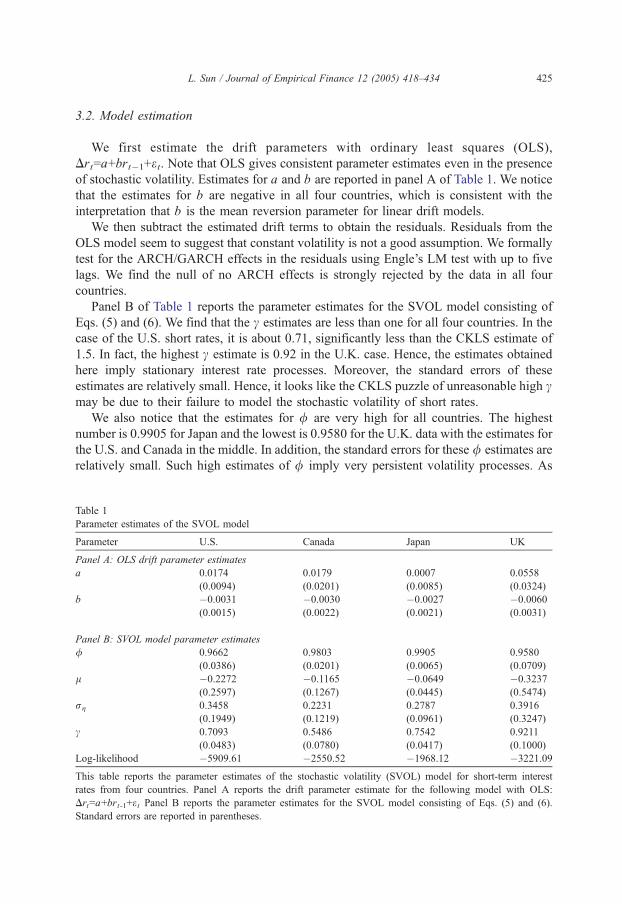
Panel B of Table 1 reports the parameter estimates for the SVOL model consisting of

Eqs. (5) and (6). We find that the c estimates are less than one for all four countries. In the

case of the U.S. short rates, it is about 0.71, significantly less than the CKLS estimate of

1.5. In fact, the highest c estimate is 0.92 in the U.K. case. Hence, the estimates obtained

here imply stationary interest rate processes. Moreover, the standard errors of these

estimates are relatively small. Hence, it looks like the CKLS puzzle of unreasonable high cmay be due to their failure to model the stochastic volatility of short rates.

We also notice that the estimates for / are very high for all countries. The highest

number is 0.9905 for Japan and the lowest is 0.9580 for the U.K. data with the estimates for

the U.S. and Canada in the middle. In addition, the standard errors for these / estimates are

relatively small. Such high estimates of / imply very persistent volatility processes. As

Table 1

Parameter estimates of the SVOL model

Parameter U.S. Canada Japan UK

Panel A: OLS drift parameter estimates

a 0.0174 0.0179 0.0007 0.0558

(0.0094) (0.0201) (0.0085) (0.0324)

b �0.0031 �0.0030 �0.0027 �0.0060

(0.0015) (0.0022) (0.0021) (0.0031)

Panel B: SVOL model parameter estimates

/ 0.9662 0.9803 0.9905 0.9580

(0.0386) (0.0201) (0.0065) (0.0709)

l �0.2272 �0.1165 �0.0649 �0.3237

(0.2597) (0.1267) (0.0445) (0.5474)

rg 0.3458 0.2231 0.2787 0.3916

(0.1949) (0.1219) (0.0961) (0.3247)

c 0.7093 0.5486 0.7542 0.9211

(0.0483) (0.0780) (0.0417) (0.1000)

Log-likelihood �5909.61 �2550.52 �1968.12 �3221.09

This table reports the parameter estimates of the stochastic volatility (SVOL) model for short-term interest

rates from four countries. Panel A reports the drift parameter estimate for the following model with OLS:

Drt=a+brt-1+e t Panel B reports the parameter estimates for the SVOL model consisting of Eqs. (5) and (6).

Standard errors are reported in parentheses.


indicated by Lamoureux and Lastrapes (1990), the pricing of contingent claims, such as

options, relies on perceptions of how permanent volatility shocks are. A transitory volatility

shock will have a smaller impact on the price of an option with a relatively long maturity,

and vice versa. Hence, correct specification of the persistence in volatility process is an

important issue at least from the perspective of pricing derivative securities.

Lamoureux and Lastrapes (1990) argue that the apparent highly persistent volatility

found with the GARCH models could be misleading if we do not account for possible

structural breaks in the volatility process. Obviously, the same criticism is also applicable

to the SVOL model used here. Therefore, we proceed by estimating the RSSV model to

account for possible regime shifts in short-rate volatility.

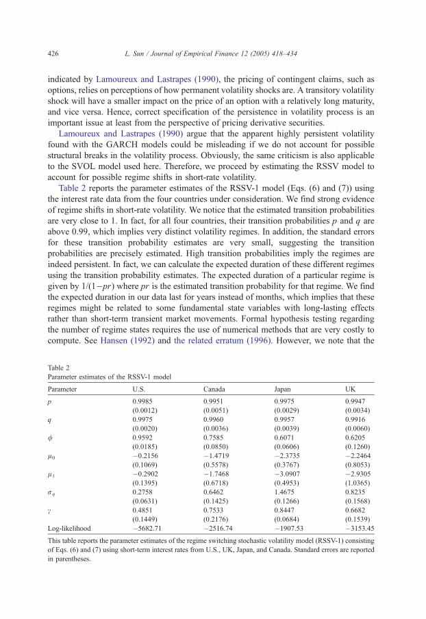
Table 2 reports the parameter estimates of the RSSV-1 model (Eqs. (6) and (7)) using

the interest rate data from the four countries under consideration. We find strong evidence

of regime shifts in short-rate volatility. We notice that the estimated transition probabilities

are very close to 1. In fact, for all four countries, their transition probabilities p and q are

above 0.99, which implies very distinct volatility regimes. In addition, the standard errors

for these transition probability estimates are very small, suggesting the transition

probabilities are precisely estimated. High transition probabilities imply the regimes are

indeed persistent. In fact, we can calculate the expected duration of these different regimes

using the transition probability estimates. The expected duration of a particular regime is

given by 1/(1�pr) where pr is the estimated transition probability for that regime. We find

the expected duration in our data last for years instead of months, which implies that these

regimes might be related to some fundamental state variables with long-lasting effects

rather than short-term transient market movements. Formal hypothesis testing regarding

the number of regime states requires the use of numerical methods that are very costly to

compute. See Hansen (1992) and the related erratum (1996). However, we note that the

Table 2

Parameter estimates of the RSSV-1 model


p 0.9985 0.9951 0.9975 0.9947

(0.0012) (0.0051) (0.0029) (0.0034)

q 0.9975 0.9960 0.9957 0.9916

(0.0020) (0.0036) (0.0039) (0.0060)

/ 0.9592 0.7585 0.6071 0.6205

(0.0185) (0.0850) (0.0606) (0.1260)

l0 �0.2156 �1.4719 �2.3735 �2.2464

(0.1069) (0.5578) (0.3767) (0.8053)

l1 �0.2902 �1.7468 �3.0907 �2.9305

(0.1395) (0.6718) (0.4953) (1.0365)

rg 0.2758 0.6462 1.4675 0.8235

(0.0631) (0.1425) (0.1266) (0.1568)

c 0.4851 0.7533 0.8447 0.6682

(0.1449) (0.2176) (0.0684) (0.1539)

Log-likelihood �5682.71 �2516.74 �1907.53 �3153.45

This table reports the parameter estimates of the regime switching stochastic volatility model (RSSV-1) consisting

of Eqs. (6) and (7) using short-term interest rates from U.S., UK, Japan, and Canada. Standard errors are reported

in parentheses.


pseudo-likelihood ratio test statistics are all extremely significant, with the highest p-value

being 8.8�10�14 in the case of Canada and lowest p-value 3.3�10�97 in the case of the

U.S. data. Alternatively, Smith (2002) proposes the use of Vuong’s (1989) likelihood ratio

(LR) test for nonnested competing models. Vuong’s test statistic is as follows:

n�1=2LRn=x̂xnYN 0; 1ð Þ;

where LRn=LnRSSV�Ln

SVOL, L is the log-likelihood value, n is the number of observations,

and x̂n2 is the variance of the LR statistic. Vuong’s LR statistic for the RSSV-1 model over

the SVOL model is as follows ( p-values in parentheses): for U.S., it is 9.9070 (0.0000); for

Canada, it is 3.7909 (0.0000); Japan 4.7885 (0.0000); U.K. 5.3340 (0.0000). Hence,

Vuong’s LR test unanimously chooses the RSSV-1 model over the SVOL model for all four

countries.

Another interesting phenomenon is related to the parameter estimates for /. If we

compare the / estimates obtained from the SVOL model versus those from the RSSV

model, we find the parameter estimates drop dramatically for three out of the four

countries. For the Canada short-rate volatility, / decreases from 0.98 to 0.76, for Japan

from 0.99 to 0.61, and for the United Kingdom from 0.96 to 0.62. These represent

decreases of 22% to 38%. In addition, the standard errors are relatively small compared

with the magnitude of the decreases. The same parameter estimates decrease slightly in the

U.S. case and are not statistically different from each other. This seems to confirm the our

concern that the SVOL model could lead to overstated volatility persistence due to its

failure to account for regime shifts in the volatility.

The c estimates are broadly similar for the two models under consideration. We note

that all the estimates of c are less than one. In other words, they all imply stationary

interest rate processes. This reaffirms that the CKLS puzzle is possibly due to model

misspecification.

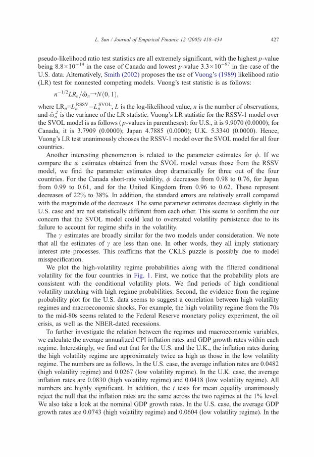
We plot the high-volatility regime probabilities along with the filtered conditional

volatility for the four countries in Fig. 1. First, we notice that the probability plots are

consistent with the conditional volatility plots. We find periods of high conditional

volatility matching with high regime probabilities. Second, the evidence from the regime

probability plot for the U.S. data seems to suggest a correlation between high volatility

regimes and macroeconomic shocks. For example, the high volatility regime from the 70s

to the mid-80s seems related to the Federal Reserve monetary policy experiment, the oil

crisis, as well as the NBER-dated recessions.

To further investigate the relation between the regimes and macroeconomic variables,

we calculate the average annualized CPI inflation rates and GDP growth rates within each

regime. Interestingly, we find out that for the U.S. and the U.K., the inflation rates during

the high volatility regime are approximately twice as high as those in the low volatility

regime. The numbers are as follows. In the U.S. case, the average inflation rates are 0.0482

(high volatility regime) and 0.0267 (low volatility regime). In the U.K. case, the average

inflation rates are 0.0830 (high volatility regime) and 0.0418 (low volatility regime). All

numbers are highly significant. In addition, the t tests for mean equality unanimously

reject the null that the inflation rates are the same across the two regimes at the 1% level.

We also take a look at the nominal GDP growth rates. In the U.S. case, the average GDP

growth rates are 0.0743 (high volatility regime) and 0.0604 (low volatility regime). In the

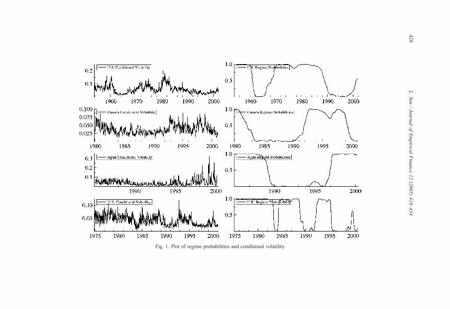
Fig. 1. Plot of regime probabilities and conditional volatility.

L.Sun/JournalofEmpirica

lFinance

12(2005)418–434

428


U.K. case, the average GDP growth rates are 0.0232 (high volatility regime) and 0.0128

(low volatility regime). Hence, it looks like the high (low) volatility regime is associated

with higher (lower) inflation and lower (higher) real GDP growth. In the cases of Japan

and Canada, the inflation rates and GDP growth rates across the regimes are statistically

indistinguishable, possibly due to their relatively short sample periods.

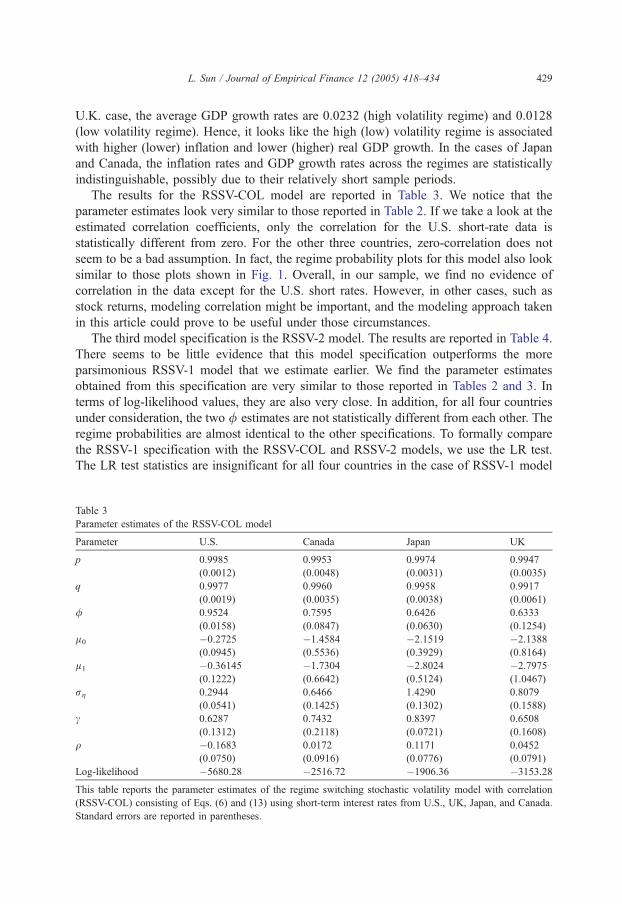
The results for the RSSV-COL model are reported in Table 3. We notice that the

parameter estimates look very similar to those reported in Table 2. If we take a look at the

estimated correlation coefficients, only the correlation for the U.S. short-rate data is

statistically different from zero. For the other three countries, zero-correlation does not

seem to be a bad assumption. In fact, the regime probability plots for this model also look

similar to those plots shown in Fig. 1. Overall, in our sample, we find no evidence of

correlation in the data except for the U.S. short rates. However, in other cases, such as

stock returns, modeling correlation might be important, and the modeling approach taken

in this article could prove to be useful under those circumstances.

The third model specification is the RSSV-2 model. The results are reported in Table 4.

There seems to be little evidence that this model specification outperforms the more

parsimonious RSSV-1 model that we estimate earlier. We find the parameter estimates

obtained from this specification are very similar to those reported in Tables 2 and 3. In

terms of log-likelihood values, they are also very close. In addition, for all four countries

under consideration, the two / estimates are not statistically different from each other. The

regime probabilities are almost identical to the other specifications. To formally compare

the RSSV-1 specification with the RSSV-COL and RSSV-2 models, we use the LR test.

The LR test statistics are insignificant for all four countries in the case of RSSV-1 model

Table 3

Parameter estimates of the RSSV-COL model


p 0.9985 0.9953 0.9974 0.9947

(0.0012) (0.0048) (0.0031) (0.0035)

q 0.9977 0.9960 0.9958 0.9917

(0.0019) (0.0035) (0.0038) (0.0061)

/ 0.9524 0.7595 0.6426 0.6333

(0.0158) (0.0847) (0.0630) (0.1254)

l0 �0.2725 �1.4584 �2.1519 �2.1388

(0.0945) (0.5536) (0.3929) (0.8164)

l1 �0.36145 �1.7304 �2.8024 �2.7975

(0.1222) (0.6642) (0.5124) (1.0467)

rg 0.2944 0.6466 1.4290 0.8079

(0.0541) (0.1425) (0.1302) (0.1588)

c 0.6287 0.7432 0.8397 0.6508

(0.1312) (0.2118) (0.0721) (0.1608)

q �0.1683 0.0172 0.1171 0.0452

(0.0750) (0.0916) (0.0776) (0.0791)

Log-likelihood �5680.28 �2516.72 �1906.36 �3153.28

This table reports the parameter estimates of the regime switching stochastic volatility model with correlation

(RSSV-COL) consisting of Eqs. (6) and (13) using short-term interest rates from U.S., UK, Japan, and Canada.

Standard errors are reported in parentheses.

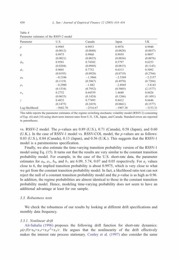
Table 4

Parameter estimates of the RSSV-2 model


p 0.9985 0.9953 0.9976 0.9940

(0.0012) (0.0048) (0.0028) (0.0037)

q 0.9975 0.9960 0.9959 0.9897

(0.0021) (0.0035) (0.0036) (0.0076)

/0 0.9581 0.74302 0.5797 0.6253

(0.0204) (0.0969) (0.0815) (0.1143)

/1 0.9601 0.7752 0.6313 0.5092

(0.0195) (0.0928) (0.0719) (0.2764)

l0 �0.2106 �1.3866 �2.5369 �2.2157

(0.1119) (0.5867) (0.4970) (0.7204)

l1 �0.2980 �1.882 �2.8945 �3.8143

(0.1534) (0.7952) (0.5805) (2.1577)

rg 0.2752 0.64559 1.4680 0.8426

(0.0633) (0.1424) (0.1266) (0.1491)

c 0.4833 0.77493 0.8412 0.6646

(0.1475) (0.2419) (0.0661) (0.1577)

Log-likelihood �5682.70 �2516.67 �1907.38 �3153.31


of Eqs. (6) and (14) using short-term interest rates from U.S., UK, Japan, and Canada. Standard errors are reported

in parentheses.


vs. RSSV-2 model. The p-values are 0.89 (U.S.), 0.71 (Canada), 0.58 (Japan), and 0.60

(U.K.). In the case of RSSV-1 model vs. RSSV-COL model, the p-values are as follows:

0.03 (U.S.), 0.84 (Canada), 0.13 (Japan), and 0.56 (U.K.). This suggests that the RSSV-1

model is a parsimonious specification.

Finally, we also estimate the time-varying transition probability version of the RSSV-1

model using Eq. (15). It turns out that the results are very similar to the constant transition

probability model. For example, in the case of the U.S. short-rate data, the parameter

estimates for a0, a1, b0, and b1 are 6.09, 5.74, 0.07 and 0.05 respectively. For aj values

close to 6, the implied transition probability is about 0.9975, which is very close to what

we get from the constant transition probability model. In fact, a likelihood ratio test can not

reject the null of a constant transition probability model and the p-value is as high as 0.96.

In addition, the regime probabilities are almost identical to those in the constant transition

probability model. Hence, modeling time-varying probability does not seem to have an

additional advantage at least for our sample.

3.3. Robustness tests

We check the robustness of our results by looking at different drift specifications and

monthly data frequency.

3.3.1. Nonlinear drift

ARt-Sahalia (1996) proposes the following drift function for short-rate dynamics:

l(r,h)=a0+a1r+a2r2+a3/r. He argues that the nonlinearity of the drift effectively

makes the interest rate process stationary. Conley et al. (1997) also consider the same


parameterization of the drift as in ARt-Sahalia (1996). Nonlinearities in the drift are

shown to be important for very high-variance elasticities (greater than 4) but not for

low ones. Similar results are also reported in Stanton (1997) and Ahn and Gao (1999).

The apparent success of nonlinear drift models, however, is inconclusive. Pritsker (1998)

questions the specification test developed in ARt-Sahalia (1996). The argument is that

interest rates are known to be highly correlated whereas the nonparametric technique used in

ARt-Sahalia’s paper is very sensitive to the dependence in the data. Chapman and Pearson

(2000) study the finite-sample properties of the nonparametric estimators used in ARt-Sahalia(1996) and Stanton (1997) by applying them to simulated sample paths of a square-root

diffusion. Although the drift is linear, the nonparametric estimators suggest nonlinearities of

the type and magnitude reported in ARt-Sahalia (1996) and Stanton (1997). Chapman and

Pearson conclude that nonlinearity of the short-rate drift is not a robust stylized fact.

To check whether our results are sensitive to the specification of the drift function. We

reestimate the RSSV model using the nonlinear drift function. The estimation technique

remains unchanged. The only difference is that we run the following regression to get the

OLS residuals:

Drt ¼ aþ brt�1 þ cr2t�1 þ dr�1t�1 þ et:

The results for the RSSV-2 model are reported in Table 5. Despite some slight differences,

the overall results continue to support the existence of two volatility regimes and they look

similar to the linear drift specification especially in the U.S. case.

3.3.2. ARIMA(1,1,0) specification

Using Box-Jenkins methods, Kalimipalli and Susmel (2004) find that an ARIMA(1,1,0)

model provides a satisfactory fit for the U.S. short rates that are highly autocorrelated. As an

additional robustness check, we reestimate our RSSV model with this ARIMA(1,1,0)

specification for the conditional mean. Namely, we obtain the OLS residuals after running

the following regression: Drt=a+bDrt�1+et. Once again, we find the results are very similar

to those reported in the previous tables.2 The transition probability estimates are still very

close to one, indicating two sharply defined volatility regimes. Hence, we conclude our

results are robust to difference drift function specifications.

3.3.3. Monthly data

Our results are derived using the weekly short-term interest rate data. As Brenner et al.

(1996) point out, the weekly data have the advantage that a discrete time approximation to

a continuous time model holds better with higher frequency data. However, the monthly

data have the advantage that 30-day bills are closer to the true short rate that the SVOL/

RSSV models are designed to analyze. In addition, a number of studies, such as Smith

(2002), use monthly U.S. short-rate data. To verify that our results are not sensitive to the

change in data frequency, we reestimate our RSSV model using the U.S. 1-month risk-free

rates (January 1954 to October 2001) obtained from CRSP. The parameter estimates for

the RSSV-2 model are as follows (standard errors in parentheses): p=0.98776 (0.02533),

2 To conserve space, we have omitted the results. All unreported results are available upon request.

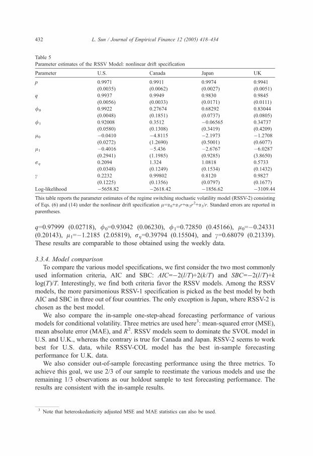
Table 5

Parameter estimates of the RSSV Model: nonlinear drift specification


p 0.9971 0.9911 0.9974 0.9941

(0.0035) (0.0062) (0.0027) (0.0051)

q 0.9937 0.9949 0.9830 0.9845

(0.0056) (0.0033) (0.0171) (0.0111)

/0 0.9922 0.27674 0.68292 0.83044

(0.0048) (0.1851) (0.0737) (0.0805)

/1 0.92008 0.3512 �0.06565 0.34737

(0.0580) (0.1308) (0.3419) (0.4209)

l0 �0.0410 �4.8115 �2.1973 �1.2708

(0.0272) (1.2690) (0.5001) (0.6077)

l1 �0.4016 �5.436 �2.6767 �6.0287

(0.2941) (1.1985) (0.9285) (3.8650)

rg 0.2094 1.324 1.0818 0.5733

(0.0348) (0.1249) (0.1534) (0.1432)

c 0.2232 0.99802 0.8120 0.9827

(0.1225) (0.1356) (0.0797) (0.1677)

Log-likelihood �5658.82 �2618.42 �1856.62 �3109.44


of Eqs. (6) and (14) under the nonlinear drift specification l=a0+a1r+a2r2+a3/r. Standard errors are reported in

parentheses.


q=0.97999 (0.02718), /0=0.93042 (0.06230), /1=0.72850 (0.45166), l0=�0.24331

(0.20143), l1=�1.2185 (2.05819), rg=0.39794 (0.15504), and c=0.68079 (0.21339).

These results are comparable to those obtained using the weekly data.

3.3.4. Model comparison

To compare the various model specifications, we first consider the two most commonly

used information criteria, AIC and SBC: AIC=�2(l/T)+2(k/T) and SBC=�2(l/T)+k

log(T)/T. Interestingly, we find both criteria favor the RSSV models. Among the RSSV

models, the more parsimonious RSSV-1 specification is picked as the best model by both

AIC and SBC in three out of four countries. The only exception is Japan, where RSSV-2 is

chosen as the best model.

We also compare the in-sample one-step-ahead forecasting performance of various

models for conditional volatility. Three metrics are used here3: mean-squared error (MSE),

mean absolute error (MAE), and R2. RSSV models seem to dominate the SVOL model in

U.S. and U.K., whereas the contrary is true for Canada and Japan. RSSV-2 seems to work

best for U.S. data, while RSSV-COL model has the best in-sample forecasting

performance for U.K. data.

We also consider out-of-sample forecasting performance using the three metrics. To

achieve this goal, we use 2/3 of our sample to reestimate the various models and use the

remaining 1/3 observations as our holdout sample to test forecasting performance. The

results are consistent with the in-sample results.

3 Note that heteroskedasticity adjusted MSE and MAE statistics can also be used.


4. Concluding remarks

In this paper, we investigate the possibility of regime shifts in short-rate volatility.

First, we find strong evidence in support of the existence of regime shifts in short-rate

volatility in four countries, particularly in the U.S. and the U.K., based on both Vuong’s

nonnested LR test, standard model selection criteria, and both in-sample and out-of-sample

forecasting performance metrics.

Second, we find parameter estimates from the SVOL model imply highly persistent

short-rate volatility for all the four countries under consideration. In contrast, we estimate

the RSSV model using the same data set and find that the previously found persistence in

volatility falls dramatically for the U.K., Canada, and Japan data. In the case of the U.S.

short-rate volatility, the volatility is still highly persistent. The evidence presented here

highlights the importance of accounting for possible structural breaks in the volatility

process.

Third, we propose several extensions of the RSSV model. In particular, we show how

to account for correlation in the RSSV model and how to estimate a time-varying

transition probability RSSV model. In our data, we find some evidence of negative

correlation for the U.S. short-rate volatility, but essentially zero-correlation for other

countries. The empirical evidence also favors the more parsimonious constant transition

probability model.

The volatility regimes identified in this paper are very distinct and seem to last for a

fairly long period of time. In the U.S. and the U.K. samples, we find that the high (low)

volatility regime is associated with higher (lower) inflation rate and lower (higher) real

GDP growth rate, which appears consistent with the notion that the regimes are related to

macroeconomic shocks.

Acknowledgements

I would like to thank Richard Baillie (editor), two anonymous referees, Bill

Lastrapes, Stewart Mayhew, Chris Stivers, Marc Lipson, Joe Sinkey, and seminar

participants at the 2003 FMA meetings for helpful comments and suggestions. All

remaining errors are my own.

References

Ahn, D.H., Gao, B., 1999. A parametric nonlinear model of term structure dynamics. Review of Financial Studies

12, 721–762.

ARt-Sahalia, Y., 1996. Testing continuous-time models of the spot interest rate. Review of Financial Studies 9,

385–426.

Ball, C., Torous, W., 1999. The stochastic volatility of short-term interest rates: some international evidence.

Journal of Finance 54, 2339–2359.

Black, F., 1976. Studies of stock price volatility changes. Proceedings of the Business and Economic Statistics.

American Statistical Association, pp. 177–181.

Bollerslev, T., 1986. Generalized autoregressive conditional heteroskedasticity. Journal of Econometrics 31,

307–327.


Brenner, R., Harjes, R., Kroner, K., 1996. Another look at models of the short-term interest rate. Journal of

Financial and Quantitative Analysis 31, 85–107.

Cai, J., 1994. A Markov model of switching-regime ARCH. Journal of Business & Economic Statistics 12,

309–316.

Chan, K., Karolyi, G., Longstaff, F., Sanders, A., 1992. An empirical comparison of alternative models of the

short-term interest rate. Journal of Finance 47, 1209–1227.

Chapman, D., Pearson, N., 2000. Is the short rate drift actually nonlinear? Journal of Finance 55, 355–388.

Chapman, D., Pearson, N., 2001. Recent advances in estimating term-structure models. Financial Analysts

Journal 57, 77–95.

Conley, T., Hansen, L., Luttmer, E., Scheinkman, J., 1997. Short-term interest rate as subordinated diffusions.

Review of Financial Studies 10, 525–577.

Cox, J., Ingersoll, J., Ross, S., 1985. A theory of the term structure of interest rates. Econometrica 53, 385–406.

Diebold, F., Lee, J., Weinbach, G., 1994. Regime switching with time-varying transition probabilities. In:

Hargreaves, C. (Ed.), Time Series Analysis and Cointegration. Oxford University Press.

Engle, R., 1982. Autoregressive conditional heteroskedasticity with estimates of the variance of U.K. inflation.

Econometrica 50, 987–1008.

Gray, S., 1996. Modeling the conditional distribution of interest rates as a regime-switching process. Journal of

Financial Economics 42, 27–62.

Hamilton, J., 1989. A new approach to the economic analysis of nonstationary time series and the business cycle.

Econometrica 57, 357–384.

Hamilton, J., Susmel, R., 1994. Autoregressive conditional heteroskedasticity and changes in regime. Journal of

Econometrics 64, 307–333.

Hansen, B., 1992. The likelihood ratio test under nonstandard conditions: testing the Markov switching model of

GNP. Journal of Applied Econometrics 7, S61–S82.

Hansen, B., 1996. Erratum: the likelihood ratio test under nonstandard conditions: testing the Markov switching

model of GNP. Journal of Applied Econometrics 11, 195–198.

Harvey, A., Shephard, N., 1996. Estimation of an asymmetric stochastic volatility model for asset returns. Journal

of Business & Economic Statistics 14, 429–434.

Harvey, A., Ruiz, E., Shephard, N., 1994. Multivariate stochastic variance models. Review of Economic Studies

61, 247–264.

Kalimipalli, M., Susmel, R., 2004. Regime-switching stochastic volatility and short-term interest rates. Journal of

Empirical Finance 11, 309–329.

Kim, C., 1994. Dynamic linear models with Markov-switching. Journal of Econometrics 60, 1–22.

Kim, C., Nelson, C., 1999. State-Space Models with Regime Switching. The MIT Press, Cambridge, MA.

Lamoureux, C., Lastrapes, W., 1990. Persistence in variance, structural change and the GARCH model. Journal of

Business & Economic Statistics 8, 225–234.

Longstaff, F., Schwartz, E., 1992. Interest rate volatility and the term structure: a two-factor general equilibrium

model. Journal of Finance 47, 1259–1282.

Pritsker, M., 1998. Nonparametric density estimation and tests of continuous time interest rate models. Review of

Financial Studies 11, 449–487.

Ruiz, E., 1994. Quasi-maximum likelihood estimation of stochastic volatility models. Journal of Econometrics

63, 289–306.

Smith, D., 2002. Markov-switching and stochastic volatility diffusion models of short-term interest rates. Journal

of Business & Economic Statistics 20, 183–197.

So, M., Lam, K., Li, W., 1998. A stochastic volatility model with Markov switching. Journal of Business &

Economic Statistics 16, 244–253.

Stanton, R., 1997. A nonparametric model of term structure dynamics and the market price of interest rate risk.

Journal of Finance 52, 1973–2000.

Taylor, S., 1986. Modelling Financial Time Series. John Wiley, Chichester, UK.

Vasicek, O., 1977. An equilibrium characterization of the term structure. Journal of Financial Economics 5,

177–188.

Vuong, Q., 1989. Likelihood ratio tests for model selection and non-nested hypotheses. Econometrica 57,

307–333.

regime shifts in interest rate volatility

Documents