reference input tracking: feedforward control s06/chapter 9 referenc… · reference input...

Chapter 9

Reference Input Tracking:feedforward control

9.1 Introduction

In previous lectures, we have discussed control designs based on actual or observer estimated statefeedback, eigenvalue (pole) assignments, as well as controllers based on internal model principle(IMP) for disturbance rejection. The control laws have in most part been derived to drive theoutput or the state to 0, (hopefully) despite disturbances etc. Very often in applications, however,we desire the output to track a reference input, i.e. if r(t) is the reference input, we would like theoutput y(t)→ r(t) as t→∞.

In these notes, we first show how the control techniques can be modified to include referenceinput.

The three methods are:

1. Internal model controller

2. Incorporating reference in state space control system

3. Feedforward control design, especially for non-minimum phase systems.

The second half of the notes will discuss a special case of feedforward controller for vibrationsuppression - known as input shaping.

9.2 Internal model controller (IMC)

Using IMP for reference tracking has already been discussed. Here, we will just illustrate it withan example.

If the reference input can be generated using a set of autonomous linear differential equation,e.g.

dnr

dtn+ an−1

dn−1r

dtn−1+ . . .+ a1

dr

dt+ a0 = 0,

then, taking Laplace transform, we can define a reference generating polynomial Γr(s) just like thatthe way we did for disturbances in class, so that

Γr(s)R(s) = Ic(s) =n∑

i=0

gir(i)(0) = terms corresponding to initial conditions.

149

150 c©Perry Y.Li

Go(s)C(s)

R(s)

Di(s) Do(s)

Y(s)

Figure 9.1: Internal Model Control for reference tracking

where r(i) denotes the i-th time derivative of r. The controller design can now proceed based onFig. 9.1 as if the reference is a disturbance. So, according to the IMP, we need the controller C(s)to incorporate the reference generating polynomial Γr(s) into its denominator:

C(s) =P (s)

Γr(s)L(s)

where P (s) and L(s) are chosen so that the closed loop system is stable.

Example: Let the plant be G(s) = 5/(s+ 1). Suppose that the reference to be tracked is

r(t) = 2sin(3t)

Since R(s) = αs/(s2 + 9), the reference generating polynomial is Γr(s) = (s2 + 9).From previous notes, we know that in order to do arbitrary pole assignment, we need the order

of the closed loop system to be at least 2n− 1 + q = 3 where n = 1 is the order of plant, q = 2 isthe order of the Γr(s). Let the controller be

C(s) =b2s

2 + b1s+ b0s2 + 9

.

and the 2n− 1 + q order closed loop characteristic polynomial is:

Acl(s) = (s+ 1)(s2 + 9) + (b2s2 + b1s+ b0) · 5. (9.1)

If we decide to place all the poles at −2, we need Acl(s) = (s+ 2)2 = s3 + 6s2 + 12s+ 8.Therefore, equating the target Acl(s) to (9.1), we choose b2 = (6 − 1)/5 = 1, b1 = (12 − 9)/5,

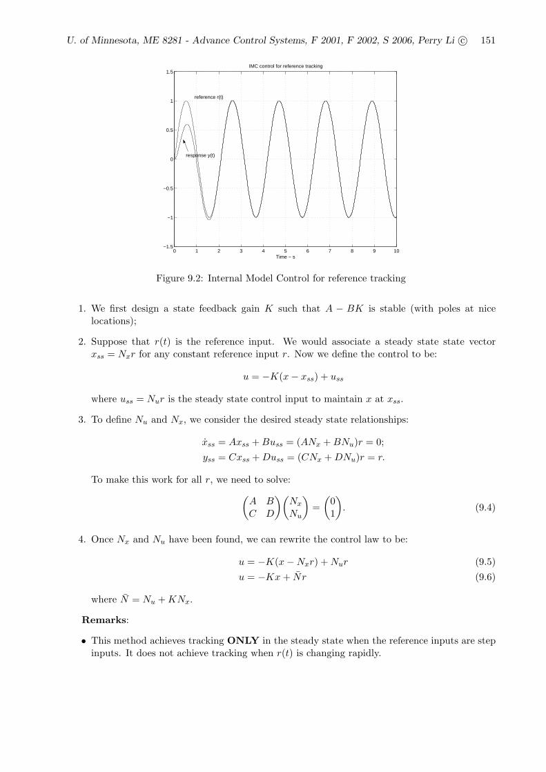
b0 = (8− 9)/5. The response is shown in Fig. 9.2.

9.3 Feedforward Control - state space method

The Internal Model Controller is appropriate if the reference input can be generated by an au-tonomous linear differential equation. In the case when the reference is fairly arbitrary, a feedfor-ward controller is needed.

First we discuss how to incorporate reference input into the state feedback controller (and byextension, observer state feedback). This method, however, only generate good tracking for slowlychanging references (i.e. d.c.)

Consider the state space system

x = Ax+Bu (9.2)

y = Cx+Du (9.3)

U. of Minnesota, ME 8281 - Advance Control Systems, F 2001, F 2002, S 2006, Perry Li c© 151

0 1 2 3 4 5 6 7 8 9 10−1.5

−1

−0.5

0

0.5

1

1.5IMC control for reference tracking

Time − s

reference r(t)

response y(t)

Figure 9.2: Internal Model Control for reference tracking

1. We first design a state feedback gain K such that A − BK is stable (with poles at nicelocations);

2. Suppose that r(t) is the reference input. We would associate a steady state state vectorxss = Nxr for any constant reference input r. Now we define the control to be:

u = −K(x− xss) + uss

where uss = Nur is the steady state control input to maintain x at xss.

3. To define Nu and Nx, we consider the desired steady state relationships:

xss = Axss +Buss = (ANx +BNu)r = 0;

yss = Cxss +Duss = (CNx +DNu)r = r.

To make this work for all r, we need to solve:

(A BC D

)(Nx

Nu

)

=

(01

)

. (9.4)

4. Once Nx and Nu have been found, we can rewrite the control law to be:

u = −K(x−Nxr) +Nur (9.5)

u = −Kx+ Nr (9.6)

where N = Nu +KNx.

Remarks:

• This method achieves tracking ONLY in the steady state when the reference inputs are stepinputs. It does not achieve tracking when r(t) is changing rapidly.

152 c©Perry Y.Li

• Even for slowly varying reference input, sinceNu andNx rely on information on the plant, theymight not be accurate. One should seriously consider adding an integrator to the system (i.e.make the controller have a pole at s = 0, enforcing IMP) to get rid of the constant reference.This can be done by augmenting the system by the extra state:

(xI

x

)

=

(0 C0 A

)(xI

x

)

+

(0B

)

u+

(10

)

r.

• In implementation, it is argued that (9.5) is more robust than (9.6). It is because variationin K does not need to be reflected in the computation of Nu in (9.5); whereas if K changesin (9.6), N needs to be changed too.

9.4 Feedforward control

If the eigenvalues are chosen to be very fast (far in the LHP), then the method above of introducingreference input in (9.5) would be quite adequate. For example, for the 1st order plant

x = −x+ u;

the state feedback with reference input r is

u = −K(x−Nx · r) +Nu · r

where (−1 11 0

)(Nx

Nu

)

=

(01

)

.

This gives Nu = Nx = 1. Or, N = kNx +Nu = k + 1.

Denote the feedforward part by r = Nr,

X(s)

R(s)= To(s) =

1

s+ (1 + k)

andX(s)

R(s)=

(1 + k)

s+ (1 + k)

In other words, N is the inversion of the plant at D.C.. If k is large, then this inversion is close tounity over a large frequency range.

The issues of using high gain feedback are stability robustness and noise amplification. So, kcannot be too large. In order to do tracking, we can design a feedback controller to be robust,and has good performance for disturbance rejection (but not necessarily for reference tracking)and noise immunity, then design a (dynamic) feedforward controller to fix the reference trackingperformance.

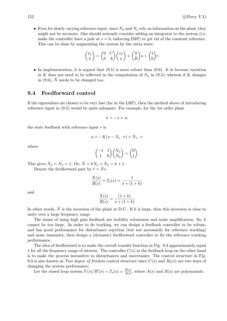
The idea of feedforward is to make the overall transfer function in Fig. 9.3 approximately equal1 for all the frequency range of interest. The controller C(s) in the feedback loop on the other handis to make the process insensitive to disturbances and uncertainty. The control structure in Fig.9.3 is also known as Two degree of freedom control structure since C(s) and H0(s) are two ways ofchanging the system performance.

Let the closed loop system Y (s)/R′(s) = To(s) = B(s)A(s) , where A(s) and B(s) are polynomials.


R(s) Y(s)

Go(s)C(s)Ho(s)R(s)

To(s)

Figure 9.3: Feedforward control concept is to make the overall transfer function Y (s)/R(s) =Ho(s)To(s) ≈ 1.

Basically, a feedforward tracking controller is to make

H0(s) =B(s)

A(s)= To(s)

−1.

This makes To(s)H0(s) = 1 so that

Y (s) = To(s)H0(s)R(s) = R(s)

Hence y(t)→ r(t) as long as To(s)H0(s) is stable.

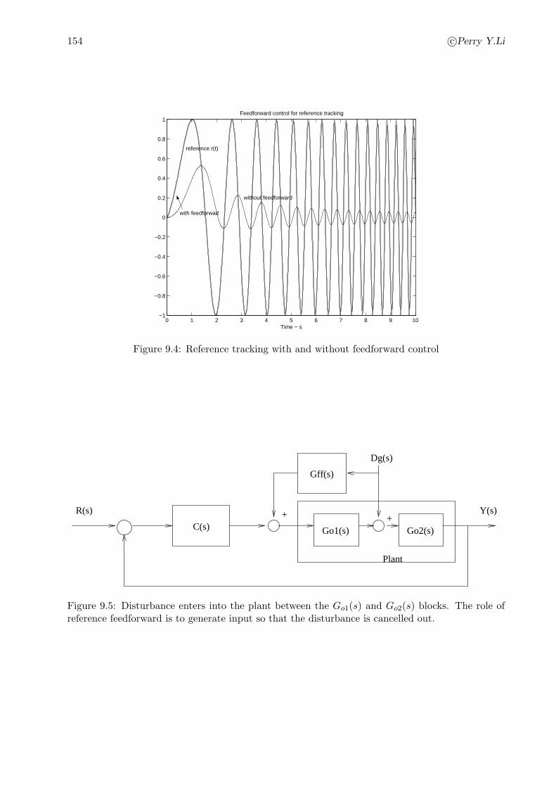
Example: Consider To(s) = 5/(s+5). This system has zero steady state tracking error for constantstep inputs. To improve tracking performance for non-constant inputs, design the feedforwardcontroller to be H0(s) = (s + 5)/5.This means that R′(s) = (0.2s + 1)R(s). Notice that this isimproper, so to actually implement this, we convert it back into time domain to get:

r′(t) = 0.2r(t) + r(t).

Fig. 9.4 shows the responses with and without H0(s). Clearly, feedforward significantly improveperformance.

There are two issues associated with the design of H0(s).

1. Notice that H0(s) generally needs to be improper - which requires derivative of r(t) to im-plement. If future r(t) is not known, derivatives are r(t) is not available (or at least notreliable). Then we need to approximate H0(s) by a proper controller. This can be done byadding terms to the denominator which only have effects at high frequencies beyond those ofinterests:

H0(s) =s+ 5

5≈ s+ 5

5(s/ω + 1)

where ω is sufficiently large to cover the frequency of interests. (see Goodwin 10.5 for anexample).

2. The second issue is if To(s) is non-minimum phase (i.e. it has poles or zeros on the unstableRHP). To(s) has to be stable, so it should not have RHP poles (if so, use C(s) to stabilizefirst). However, it can have RHP zeros, i.e. there exists z ∈ RHP such that B(z) = 0. Adirect inversion would create an unstable pole in H0(s), which is not allowed (the unstablepole is unobservable). This is dealt with by the Zero Phase Tracking Controller (ZPETC),which will be discussed next.

154 c©Perry Y.Li

0 1 2 3 4 5 6 7 8 9 10−1

−0.8

−0.6

−0.4

−0.2

0

0.2

0.4

0.6

0.8

1Feedforward control for reference tracking

Time − s

reference r(t)

with feedforwad

without feedforward

Figure 9.4: Reference tracking with and without feedforward control

C(s)

R(s) Y(s)

Go2(s)Go1(s)

Dg(s)

Gff(s)

+ +

Plant

Figure 9.5: Disturbance enters into the plant between the Go1(s) and Go2(s) blocks. The role ofreference feedforward is to generate input so that the disturbance is cancelled out.


9.4.1 Disturbance Feedforward

While future information of disturbances may not be known, the disturbance at a present time cansometimes be measured. This can be used to generate command input that cancels out its effect.

For example in Fig. 9.5, to generate the control to cancel out Dg(s), we need:

Go1(s)Gff (s)Dg(s) ≈ −Dg(s) ⇒ Go1(s)Gff (s) ≈ −1.

• Gff (s) acts in open loop, so it must be stable.

• Since future disturbances are unknown Gff (s) should be proper. We can introduce excesspoles at high frequency:

Gff (s) = − G−1o1 (s)

(s/ω + 1)nδ

where nδ is the relative degree of Go(s), and ω is large (e.g. a few times maximum bandwidthof Dg(s)).

• Since Go1(s) usually has low pass characteristics, Gff (s) will have high pass characteristics.

• Reference feedforward is particularly helpful in improving transient response when Go2(s) haslong time lag. This is the case even if an IMP controller is used, since the IMP controllercannot generate corrective action until error has been generated. The feedforward actionreacts immediately to detection of disturbances.

9.4.2 Zero-phase error tracking controller (ZPETC) - continuous time

If To(s) is stable but non-minimum phase, then we would like to design H0(s) such that

H0(s)To(s) ≈ 1

with the restriction that H0(s) is stable.

Consider for example

To(s) =(s+ 3)(s− 2)

(s+ 4)(s+ 1)

which is non-minimum phase. Let us write

To(s) =B+(s)B−(s)

A(s)

where B+(s) denotes terms with LHP roots (minimum phase part) and B−(s) denotes terms withRHP roots (non-minimum phase part). In our example, B+(s) = (s+ 3), B− = (s− 2).

One possibility (not recommended) is to choose

H0(s) =A(s)

B+(s)

±1

B−1(−s) =(s+ 4)(s+ 1)

s+ 3

±1

s+ 2.

(i.e. reflect the non-minimum phase zero on the jw axis). This makes

To(s)H0(s) = ± B−(s)

B−(−s) = −s− 2

s+ 2

156 c©Perry Y.Li

0.2 0.4 0.6 0.8 1 1.2 1.4 1.6 1.8 2

x 104

−1

−0.5

0

0.5

1

Time samples (0.0001s)

Res

pons

es o

f fee

dfor

war

d ex

ampl

e

all pass

Zpetc

no feedforward

reference

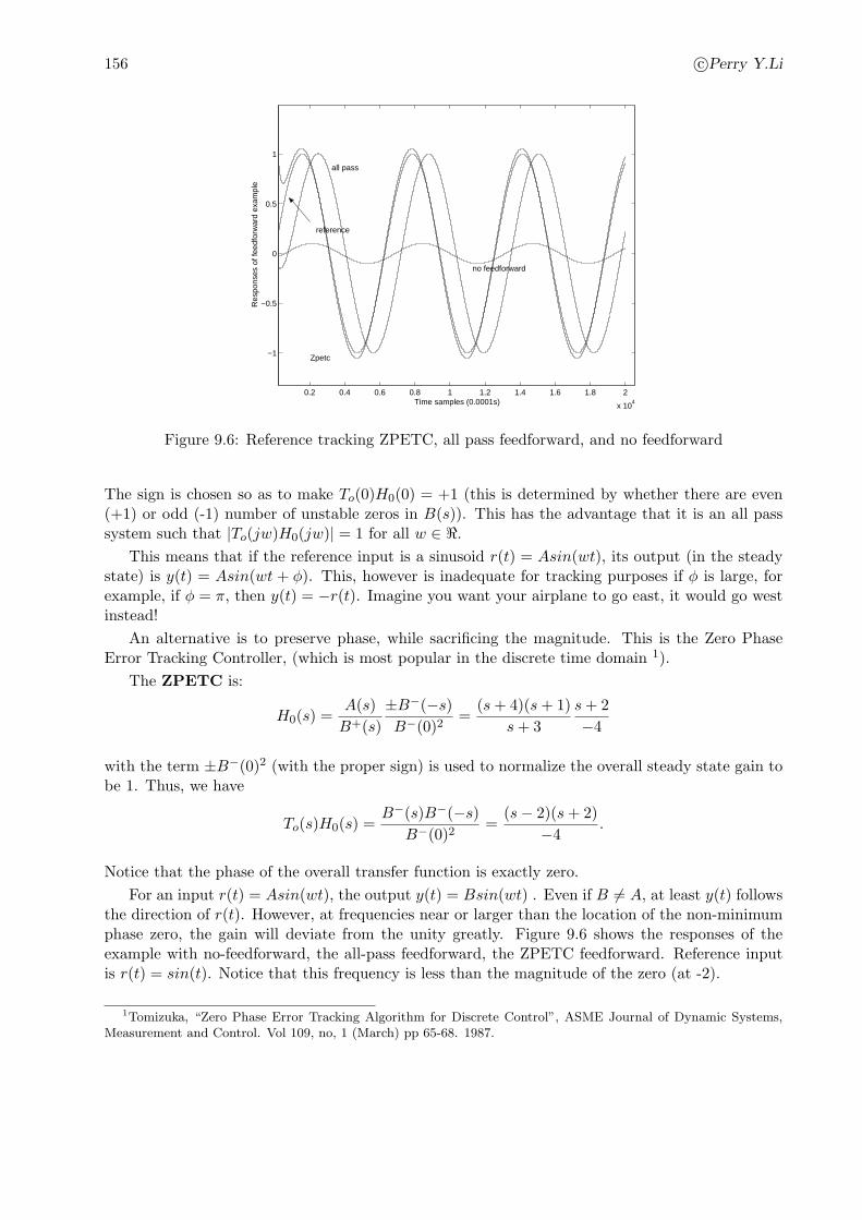
Figure 9.6: Reference tracking ZPETC, all pass feedforward, and no feedforward

The sign is chosen so as to make To(0)H0(0) = +1 (this is determined by whether there are even(+1) or odd (-1) number of unstable zeros in B(s)). This has the advantage that it is an all passsystem such that |To(jw)H0(jw)| = 1 for all w ∈ ℜ.

This means that if the reference input is a sinusoid r(t) = Asin(wt), its output (in the steadystate) is y(t) = Asin(wt + φ). This, however is inadequate for tracking purposes if φ is large, forexample, if φ = π, then y(t) = −r(t). Imagine you want your airplane to go east, it would go westinstead!

An alternative is to preserve phase, while sacrificing the magnitude. This is the Zero PhaseError Tracking Controller, (which is most popular in the discrete time domain 1).

The ZPETC is:

H0(s) =A(s)

B+(s)

±B−(−s)B−(0)2

=(s+ 4)(s+ 1)

s+ 3

s+ 2

−4

with the term ±B−(0)2 (with the proper sign) is used to normalize the overall steady state gain tobe 1. Thus, we have

To(s)H0(s) =B−(s)B−(−s)

B−(0)2=

(s− 2)(s+ 2)

−4.

Notice that the phase of the overall transfer function is exactly zero.

For an input r(t) = Asin(wt), the output y(t) = Bsin(wt) . Even if B 6= A, at least y(t) followsthe direction of r(t). However, at frequencies near or larger than the location of the non-minimumphase zero, the gain will deviate from the unity greatly. Figure 9.6 shows the responses of theexample with no-feedforward, the all-pass feedforward, the ZPETC feedforward. Reference inputis r(t) = sin(t). Notice that this frequency is less than the magnitude of the zero (at -2).

1Tomizuka, “Zero Phase Error Tracking Algorithm for Discrete Control”, ASME Journal of Dynamic Systems,Measurement and Control. Vol 109, no, 1 (March) pp 65-68. 1987.


9.5 ZPETC in discrete time

Here we consider a discrete time closed loop plant model given by:

To(q−1) =

q−δBo(q−1)

Ao(q−1)=q−δB+

o (q−1)B−o (q−1)

Ao(q−1)

where Ao(q−1) and B+

o (q−1) are stable, and

B−o (q−1) = Πm

i=1(1− βiq−1), |βi| ≥ 1.

B+o (q−1) and B−

o (q−1) are the minimum phase and non-minimum phase parts of the numerator ofTo(q

−1). As usual, we use q−1 to denote the 1 step delay (shift) operator.

As noted in previous notes on discrete time systems, the roots of the polynomial

A(q−1) = Πi(1− αiq−1)

are the complex numbers αi’s. If |αi| < 1, then signal y(k) that satisfies: A(q−1)[y(k)] = 0 wouldconverge to 0. Therefore, we say that To(q

−1) is stable if A(q−1) has all roots |αi| < 1; it has anon-minimum phase zero at β if B(β−1) = 0 and |β| > 1. We put all such factors (1 − β−j q−1)

where |β−| > 1 in B−o (q−1).

If the non-minimum phase part is trivial, i.e. B−o (q−1) = 1. Then we can design

Ho(q−1) =

qδAo(q−1)

B+o (q−1)

This usually requires that Ho(q−1) is not proper. This means that the control requires preview of

δ steps future information of the reference signal. This is okay since reference signal in many casesare known before hand.

If B−o (q−1) is non-trivial, then we cannot put B−(q−1) in the denominator of Ho(q

−1) since itwould make the controller unstable. We can use the ZPETC approach similar to the continuoustime case instead, which is explained now.

First, we note that for a discrete time system G(q−1), given a sinusoidal input of frequency ω,the in the steady state the steady state output is also sinusoidal, with a magnitude gain and phaseshift given by

|G(q−1)| and phase(G(q−1)

with evaluated at q = ejωTs where Ts is the sampling time.

Therefore, if we design the feedforward controller to be:

Ho(q−1) =

qδAo(q−1)

B+o (q−1)

B−o (q)

B−o (1)2

then, To(q−1)Ho(q

−1) becomes:

B−o (q)B−

o (q−1)

B−o (1)2

First notice that this is a polynomial in q and q−1 in the form:

γ0 + γ1(q + q−1) + γ2(q2 + q−2) + . . .

158 c©Perry Y.Li

where γk are real coefficients - i.e. the the q−k and qk terms have the same coefficients. Because ofthis, when To(q

−1)Ho(q−1) is evaluated at q ← ejωTs , the result is a real number. Hence, the phase

is zero.Second, notice that the gain of To(q

−1)Ho(q−1) is unity when q = 1 (i.e. unity gain at D.C.).

At high frequencies, gain can differ from unity significantly. If the non-minimum phase zero β hasnegative real part, then, the corresponding terms in B−

o (q)B−o (q−1) would contribute to decreasing

gain at high frequencies (ω → π/Ts). If they have positive real parts, then they would contributeto increasing gain at high frequencies. To see this, consider β is real:

(1− βq−1)(1− βq)∣∣q=ejωTs

= (1 + β2)− 2βcos(ωTs)

Hence, if β > 0, this is an increasing function of ω; and if β < 0, this is a decreasing function ω.Similar reasonings can be applied to complex β by considering the terms due to the conjugatesalso.

9.6 Non-minimum phase tracking using series expansion

The difficulty in designing feedforward controller for a discrete time non-minimum phase zero (sayat q = −2) is that, the inverse of B−

o (q−1) = (1 + 2q−1)

1

1 + 2q−1

is unstable in the forward time. The idea is to approximate this as a series in positive powers of q:

1

1 + 2q−1≈ a0 + a1q + q2q

2 + . . . anqn =: Ho(q

−1)

Notice that the right hand side means that this is non-causal finite impulse response filter thatrequires n step preview of the reference signal since,

r(k) = Ho(q−1)[r(k)] = a0r(k) + a1r(k + 1) + a2r(k + 2) + . . . anr(k + n).

To get the expansion, we can use long division (see class notes):

1

2q−1 + 1≈ 1

2q − 1

4q2 +

1

8q3 + . . .± 1

2nqn =: Ho(q

−1)

Because of the long division computation, we see easily that expansion to the qn term of (1−βq−1)results in:

(1− βq−1)Ho(q−1) = 1 +

qn

βn

where the second term represents the error from the ideal feedforward control. Since |β| > 1 byassumption (non-minimum phase), |βn| → 0 as n→∞.

One can choose n so that with q = ejωTs , 1+ qn

βn is close to 1 for both the magnitude and phase.See (Gross, Messner, Tomizuka paper) for a graphical way of interpreting this error.

Notice also that the sequence of coefficients of the series expansion is in fact the impulse responseof 1/(1− βq−1) when marching in reverse time k = 0,−1,−2, . . .:

(1− βq−1)[e(k)] = δ(k)⇒ e(k − 1) =−1

β(δ(k)− e(k))


0 0.2 0.4 0.6 0.8 1 1.2 1.4

−0.6

−0.4

−0.2

0

0.2

0.4

0.6

Frequency response of compensated non−minimum phase system − B−(q−1)= 1 + 2 q−1

ZPETCSeries 3 termsSeries 4 terms

40 50 60 70 80

−1

−0.8

−0.6

−0.4

−0.2

0

0.2

0.4

0.6

0.8

1 Desired4 terms seriesZPETC

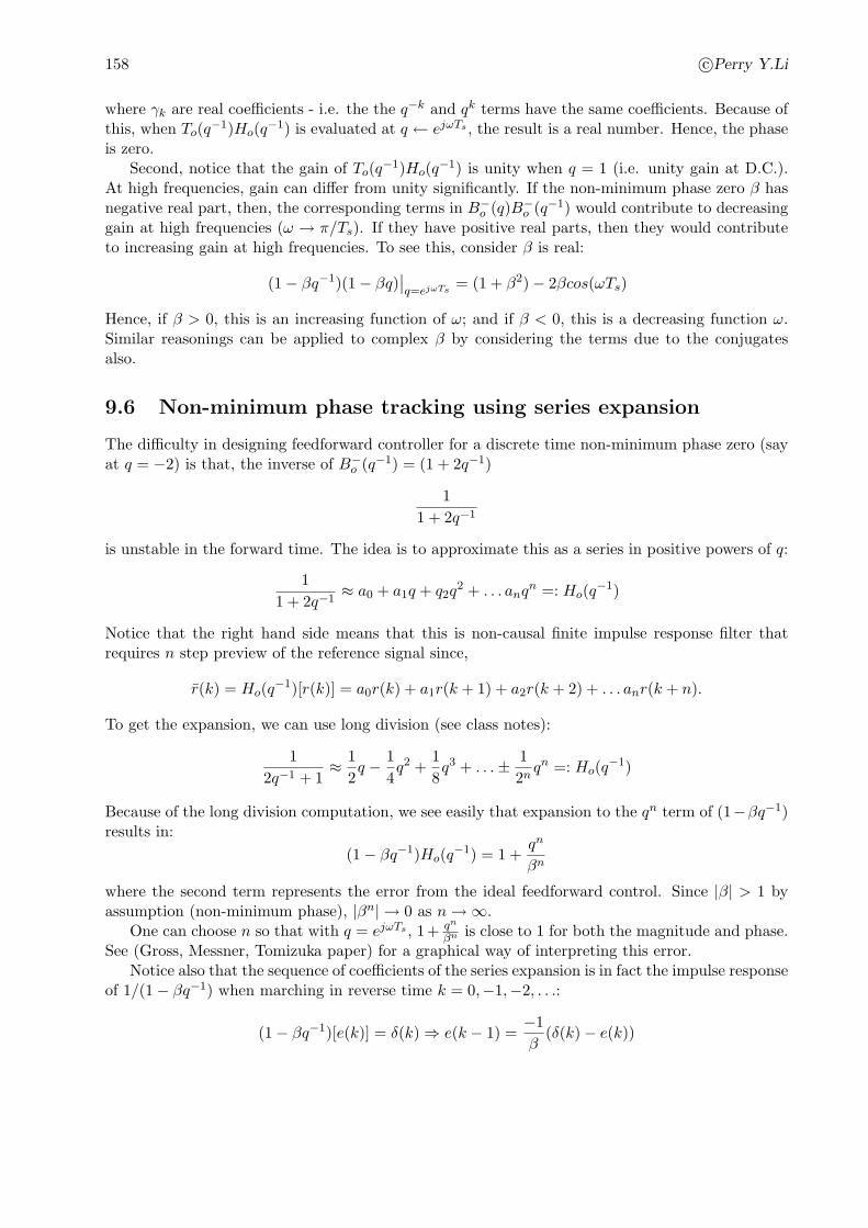
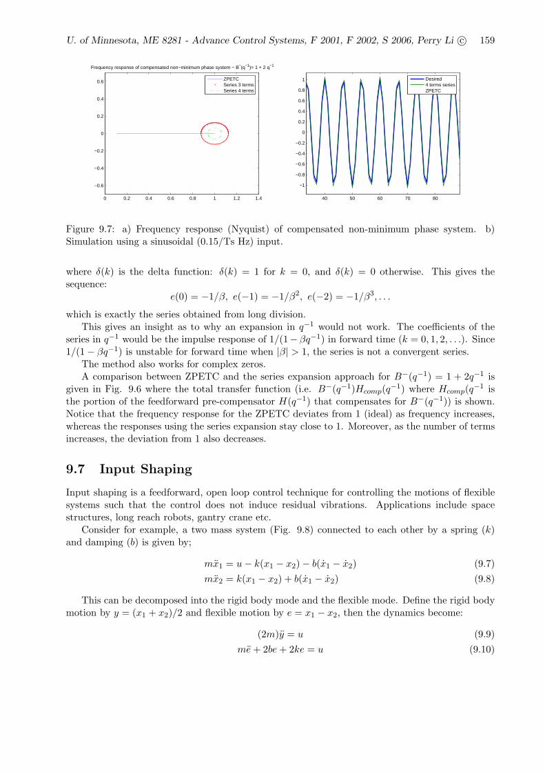
Figure 9.7: a) Frequency response (Nyquist) of compensated non-minimum phase system. b)Simulation using a sinusoidal (0.15/Ts Hz) input.

where δ(k) is the delta function: δ(k) = 1 for k = 0, and δ(k) = 0 otherwise. This gives thesequence:

e(0) = −1/β, e(−1) = −1/β2, e(−2) = −1/β3, . . .

which is exactly the series obtained from long division.This gives an insight as to why an expansion in q−1 would not work. The coefficients of the

series in q−1 would be the impulse response of 1/(1− βq−1) in forward time (k = 0, 1, 2, . . .). Since1/(1− βq−1) is unstable for forward time when |β| > 1, the series is not a convergent series.

The method also works for complex zeros.A comparison between ZPETC and the series expansion approach for B−(q−1) = 1 + 2q−1 is

given in Fig. 9.6 where the total transfer function (i.e. B−(q−1)Hcomp(q−1) where Hcomp(q

−1 isthe portion of the feedforward pre-compensator H(q−1) that compensates for B−(q−1)) is shown.Notice that the frequency response for the ZPETC deviates from 1 (ideal) as frequency increases,whereas the responses using the series expansion stay close to 1. Moreover, as the number of termsincreases, the deviation from 1 also decreases.

9.7 Input Shaping

Input shaping is a feedforward, open loop control technique for controlling the motions of flexiblesystems such that the control does not induce residual vibrations. Applications include spacestructures, long reach robots, gantry crane etc.

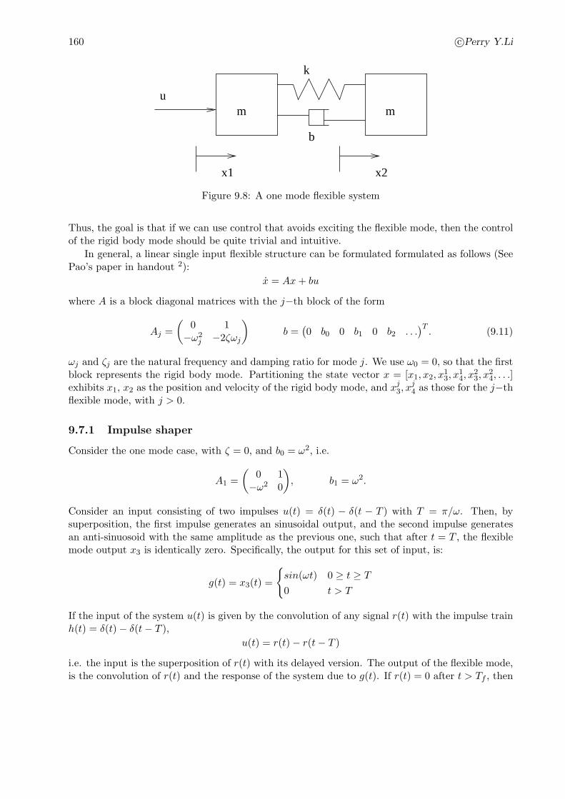
Consider for example, a two mass system (Fig. 9.8) connected to each other by a spring (k)and damping (b) is given by;

mx1 = u− k(x1 − x2)− b(x1 − x2) (9.7)

mx2 = k(x1 − x2) + b(x1 − x2) (9.8)

This can be decomposed into the rigid body mode and the flexible mode. Define the rigid bodymotion by y = (x1 + x2)/2 and flexible motion by e = x1 − x2, then the dynamics become:

(2m)y = u (9.9)

me+ 2be+ 2ke = u (9.10)

160 c©Perry Y.Li

m mu

x1 x2

k

b

Figure 9.8: A one mode flexible system

Thus, the goal is that if we can use control that avoids exciting the flexible mode, then the controlof the rigid body mode should be quite trivial and intuitive.

In general, a linear single input flexible structure can be formulated formulated as follows (SeePao’s paper in handout 2):

x = Ax+ bu

where A is a block diagonal matrices with the j−th block of the form

Aj =

(0 1−ω2

j −2ζωj

)

b =(0 b0 0 b1 0 b2 . . .

)T. (9.11)

ωj and ζj are the natural frequency and damping ratio for mode j. We use ω0 = 0, so that the firstblock represents the rigid body mode. Partitioning the state vector x = [x1, x2, x

13, x

14, x

23, x

24, . . .]

exhibits x1, x2 as the position and velocity of the rigid body mode, and xj3, x

j4 as those for the j−th

flexible mode, with j > 0.

9.7.1 Impulse shaper

Consider the one mode case, with ζ = 0, and b0 = ω2, i.e.

A1 =

(0 1−ω2 0

)

, b1 = ω2.

Consider an input consisting of two impulses u(t) = δ(t) − δ(t − T ) with T = π/ω. Then, bysuperposition, the first impulse generates an sinusoidal output, and the second impulse generatesan anti-sinuosoid with the same amplitude as the previous one, such that after t = T , the flexiblemode output x3 is identically zero. Specifically, the output for this set of input, is:

g(t) = x3(t) =

{

sin(ωt) 0 ≥ t ≥ T0 t > T

If the input of the system u(t) is given by the convolution of any signal r(t) with the impulse trainh(t) = δ(t)− δ(t− T ),

u(t) = r(t)− r(t− T )

i.e. the input is the superposition of r(t) with its delayed version. The output of the flexible mode,is the convolution of r(t) and the response of the system due to g(t). If r(t) = 0 after t > Tf , then


2 Impulse Shaper

unshaped command

Input due to 1st impulse

t2

0T

T+t2

Input due to 2nd impulse

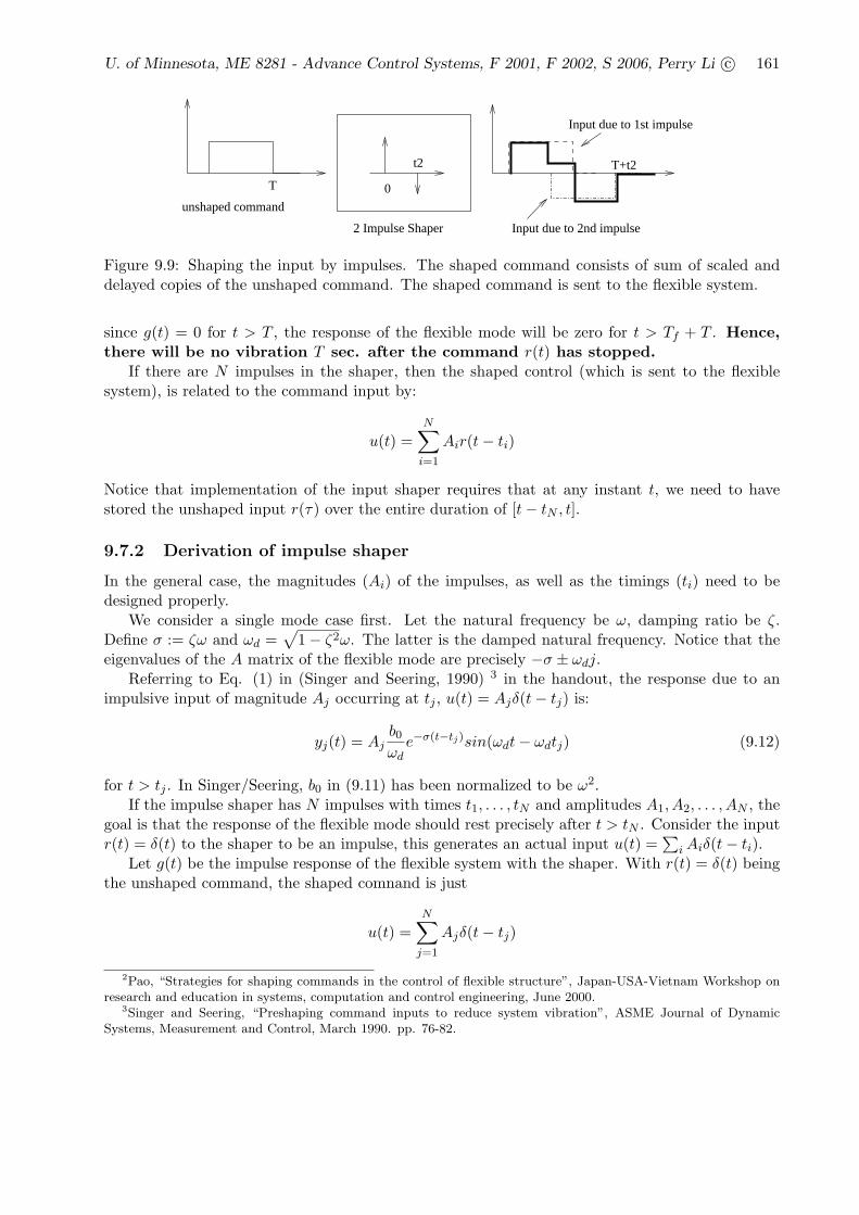
Figure 9.9: Shaping the input by impulses. The shaped command consists of sum of scaled anddelayed copies of the unshaped command. The shaped command is sent to the flexible system.

since g(t) = 0 for t > T , the response of the flexible mode will be zero for t > Tf + T . Hence,there will be no vibration T sec. after the command r(t) has stopped.

If there are N impulses in the shaper, then the shaped control (which is sent to the flexiblesystem), is related to the command input by:

u(t) =

N∑

i=1

Air(t− ti)

Notice that implementation of the input shaper requires that at any instant t, we need to havestored the unshaped input r(τ) over the entire duration of [t− tN , t].

9.7.2 Derivation of impulse shaper

In the general case, the magnitudes (Ai) of the impulses, as well as the timings (ti) need to bedesigned properly.

We consider a single mode case first. Let the natural frequency be ω, damping ratio be ζ.Define σ := ζω and ωd =

√

1− ζ2ω. The latter is the damped natural frequency. Notice that theeigenvalues of the A matrix of the flexible mode are precisely −σ ± ωdj.

Referring to Eq. (1) in (Singer and Seering, 1990) 3 in the handout, the response due to animpulsive input of magnitude Aj occurring at tj , u(t) = Ajδ(t− tj) is:

yj(t) = Ajb0ωde−σ(t−tj)sin(ωdt− ωdtj) (9.12)

for t > tj . In Singer/Seering, b0 in (9.11) has been normalized to be ω2.If the impulse shaper has N impulses with times t1, . . . , tN and amplitudes A1, A2, . . . , AN , the

goal is that the response of the flexible mode should rest precisely after t > tN . Consider the inputr(t) = δ(t) to the shaper to be an impulse, this generates an actual input u(t) =

∑

iAiδ(t− ti).Let g(t) be the impulse response of the flexible system with the shaper. With r(t) = δ(t) being

the unshaped command, the shaped comnand is just

u(t) =N∑

j=1

Ajδ(t− tj)

2Pao, “Strategies for shaping commands in the control of flexible structure”, Japan-USA-Vietnam Workshop onresearch and education in systems, computation and control engineering, June 2000.

3Singer and Seering, “Preshaping command inputs to reduce system vibration”, ASME Journal of DynamicSystems, Measurement and Control, March 1990. pp. 76-82.

162 c©Perry Y.Li

so that the response of the flexible system is for (t > tN )

g(t) =N∑

j=1

yj(t). (9.13)

where yj(t) is the response of the flexible system due to each Ajδ(t− tj) in u(t). Rewrite

yj(t) =b0ωde−σ(t−tN )Aje

−σ(tN−tj)sin(ωdt− ωdtj)

Notice that the impulse response of the shaper + flexible mode, g(t) is of the form

g(t) =b0ωde−σ(t−tN )

∑

i

Bisin(ωd(t− ti)

where Bj = Aje−σ(tN−tj). Using sin(a + b) = cos(b)sin(a) + sin(b)cos(a), we have (Eq. (2) in

Singer / Seering),

B1sin(ωdt+ φ1) +B2sin(ωdt+ φ2) + . . . = Aampsin(ωdt+ ψ)

for some Aamp and ψ (formulae given in paper), g(t) can be expressed as a decaying sinusoid

g(t) =b0ωde−σ(t−tN )Aampsin(ωd(t− ti) + ψ).

Thus, to ensure that there will be no or little vibration after the last impulse at tN , we must haveAamp ≈ 0, which is the amplitude at t = tN .

Aamp can be expressed in a different way as shown in Eq. (2) in Pao’s paper in the handout.

V (ω, ζ) = eζtN

(N∑

i=1

Aieσticos(ωdti)

)2

+

(N∑

i=1

Aieσtisin(ωdti)

)2

1

2

. (9.14)

where σ = ζω (magnitude of real part of the pole) and ωd =√

1− ζ2ω (damped natural frequency).To make V (ω, ζ) = 0, we need to make both terms inside the bracket 0, i.e.

N∑

i=1

Aieσticos(ωdti) = 0 (9.15)

N∑

i=1

Aieσtisin(ωdti) = 0 (9.16)

Example: (1 mode ZV) For a one mode case, we can choose the 1st impulse to occur at t1 = 0.We use two impulses to set (9.15)-(9.16) identically zero at ω and ζ which are the estimated naturalfrequency and damping ratio. Shapers designed this way are called ZV (zero-vibration) shapers.

The equations that need to be solved (for A1, A2 and t2) are:

A1 +A2eσt2cos(ωdt2) = 0 (9.17)

A2eσt2sin(ωdt2) = 0 (9.18)


This means that t2 = 0, π/ωd, 2π/ωd, . . .. The non-trivial case with the smallest t2 is t2 = π/ωd

t2 =π

ωdA2 = A1e

−σt2

Normalizing so that A1 +A2 = 1, the impulse response of the shaper is:

h(t) =1

1 + e−σt2δ(t) +

e−σt2

1 + e−σt2δ(t− π/ωd).

If we had chosen t2 = 0, then we must have A2 = −A1 so that the shaper is identically zero. If wehad chosen t2 larger, then the shaper will take a longer time for the vibration to stop.

Generally, making (9.15)-(9.16) zero involves solving a set of nonlinear equations.

9.7.3 Saturation constraints

Often one would have input limits. It is desirable that if |r(t)| < usat satisfies saturation limits,the shaped input u(t) does also. This can be guaranteed if all Ai > 0 and

N∑

i

= Ai ≤ 1.

It is because:

|u(t)| = |∑

i

Air(t− ti)| ≤∑

i

Ai|r(t− ti)| ≤∑

i

Ai|usat.

9.7.4 Robustness

To ensure that the shaper works well for inaccurate estimates of ω and ζ, Eq.(9.14) should be smalleven in these cases.

ZVD is the shaper that, in addition to making (9.14) zero at the estimated ω and ζ, it makesits partial derivatives also zero, (hence D in ZVD). (see Fig. 2 in Pao). This generates 2 additionalconstraint equations. Hence we need at least 1 more impulse at t3 and magnitude A3.

Remark

• In Singer / Seering, it is stated that making the derivative with respect to ω zero, automati-cally makes the derivative w.r.t. ζ zero.

• It is possible to generate second derivative constraints etc. to generate ZVDD, ZVDDD etc.Each “D” would generate two additional constraints, and hence 1 more impulse. Alternatively,one can make the V (ω, ζ) = 0 at frequency on either side of the design frequency. These arethe EI shapers.

• The penalty of robustness is that one needs more impulses, and hence longer time beforevibration stops.

164 c©Perry Y.Li

9.7.5 Multi-mode shaper

When there are multiple flexible modes, then one can design a shaper for each, and then convolvethem together. If we use a N impulse shaper for each mode and there are n modes, then thecomposite shaper will have Nn impulses. The last impulse would occur at t =

∑nj=1 t

jN where tNj

is the time for the last impulse for the j−th mode.Alternatively, one can simultaneously solve V (ω, ζ) in Eq.(9.14) to be 0 at all n pairs of (ωi, ζi).

To design the basic n mode ZV involves solving 2n nonlinear equations (i.e. need at least n+1impulses). This method would likely get a set of impulses that finish at a shorter amount of time.

9.7.6 Transfer function interpretation

The transfer function of the shaper

h(t) =N∑

j=1

Ajδ(t− tj)

is given by:

H(s) =N∑

j=1

Aje−stj .

Consider the 2 impulse ZV shaper in the earlier example with A2 = A1e−σt2 , t2 = π/ωd, where

σ = ζω, and ωd =√

1− ζ2ω. Then,

H(s) = A1(1 + e−σte−st2)

Notice that H(s) = 0 occurs when e−(s+σ)t2 = −1 or (s + σ)t2 = ±πj. Hence, the zeros of H(s)are at s = −σ ± π/t2 = −σ ± ωdj, which are exactly the poles of the flexible system!

This fact can be generalized (see Fig. 3 in (Pao, 2000)).

• ZV shapers place zeros at the flexible mode

• ZVD shapers place two zeros at the flexible mode

• ZI shapers place two zeros close to the flexible mode.

This insight implies that we can generate a ZVD by convolving 2 ZV. For example, the 3impulse ZVD in Fig. 4 of Singer / Seering, is the normalized convolution of the 2 impulse ZV inFig. 2.

The input shaper does not have any poles - notice that |H(s)| does not become infinity forany finite s. This is quite obvious given that the impulse response of the shaper H(s) has finiteduration.

reference input tracking: feedforward control s06/chapter 9 referenc… · reference input...

Documents