reduced order modeling of parameterized and distributed systems luca daniel, m.i.t

Reduced Order Modeling of Reduced Order Modeling of Parameterized and Distributed SystemsParameterized and Distributed Systems

Luca Daniel, M.I.T.

2

Parameterized Model Order ReductionParameterized Model Order Reduction

Problem Classification

Reducing Linear Systems

Moment Matching with Linear parameters

Moment Matching with NON-linear parameters

Quasi Convex Optimization approach

Reducing NON-linear systems


106

107

108

109

1010

100

101

102

103

104

frequency

|Z(f)|

Field solvers can produce instance impedance vs. frequency curves.

Motivation.Motivation. Example: Analysis of RF micro-inductor Example: Analysis of RF micro-inductor

How are the substrate eddy currents affecting the quality factor of the inductor?

How are the displacement currents affecting the resonance of the inductor?

Need to capture all 2nd order effects

“Model Order Reduction” can help verify how the inductor performance (Q, resonance position, etc) affect the transceiver performance (distortion, interference rejection etc.)

Modeling Requirements: as accurate as a field solver automatic and robust model compatible with circuit

simulators

MotivationMotivation Example: MOR of RF micro-inductor Example: MOR of RF micro-inductor

LNA

ADC

ADC

I

Q

LO

MotivationMotivation Example: Parameterized MOR of RF micro-inductor Example: Parameterized MOR of RF micro-inductor

LNA

ADC

ADC

I

Q

LOd

W

“Model Order Reduction” can help verify how the resonator or inductor performance (noise, quality factor, etc) affect the transceiver performance (distortion, interference rejection)

“Parameterized Model Order Reduction” can help verify how the transceiver performance changes when I change wire widths and wire separation

Luca Daniel15 July, 2003 6http://www.rle.mit.edu/cpgfrequency [Hz]frequency [Hz]

MotivationMotivationExample. Analysis of Integrated Power ElectronicsExample. Analysis of Integrated Power Electronics

How is the How is the magnetic fringing fieldmagnetic fringing field from the from the core effecting eddy current losses?core effecting eddy current losses?Analysis toolsAnalysis tools can produce for instance can produce for instance resistance vs. frequency curves.resistance vs. frequency curves.

Spattered laminated NiFe core, electroplated Spattered laminated NiFe core, electroplated windings [Daniel96]windings [Daniel96]

Rac

Luca Daniel15 July, 2003 7http://www.rle.mit.edu/cpg

Micro-inductor in a DC/DC power converterMicro-inductor in a DC/DC power converter

• ““Model Order Reduction”Model Order Reduction” can help verifying how the 2 can help verifying how the 2ndnd order effects order effects of the power inductor (e.g. power loss vs. freq. curve)of the power inductor (e.g. power loss vs. freq. curve) influences the influences the power converter functionality (dynamics, overall power efficiency)power converter functionality (dynamics, overall power efficiency)

• ““Parameterized Model Order Reduction”Parameterized Model Order Reduction” can help verify how the can help verify how the functionality and the efficiency of the overall power converter functionality and the efficiency of the overall power converter changeschanges when I change wire widths and wire separations?when I change wire widths and wire separations?

Vin(t)

Vout(t)

8

d

W

From Field Solvers From Field Solvers to Parameterized Model Order Reduction (PMOR).to Parameterized Model Order Reduction (PMOR).

dt

dEH

dt

dHE

1M equations

)()(),( tuBtxdt

dxdWE

10 equations

)(ˆ)(ˆˆ

),(ˆ tuBtxdt

xddWE

PMORPMOR

Field Solvers discretize Field Solvers discretize geometry and produce large geometry and produce large systemssystems

PMOR produces a dynamical model: PMOR produces a dynamical model:

– automaticallyautomatically

– match port impedance match port impedance

– small (10-15 ODEs)small (10-15 ODEs)

Parameterized model order reduction.Parameterized model order reduction.Problem classification Problem classification

)()(),...,,( 21 tuBtxdt

dxsssE p

linearity

matrix size

# parameters

10

Parameterized Model Order ReductionParameterized Model Order ReductionProblem ClassificationProblem Classification

matrix size

# parameters

linearity

Non-Linear SystemsLinear Time Invariant

linearlyparameterized

non-linearly parameterized

0,...,,,,, 21 pdt

dx sssuxE)()(),,( 1 tuBtxdt

dxssE p

)()(...2211 tuBtxdt

dxEsEsEs pp

)()(),...,,( 21 tuBtxdt

dxsssE p

11

Parameterized Model Order Reduction.Parameterized Model Order Reduction.ApplicationsApplications

interconnectRF inductors

matrix size

# parameters

linearity



Linear Time Invariant Non-Linear Systems

LOLNA ADC

MEMS

Packages

12

Parameterized Model Order Reduction.Parameterized Model Order Reduction.Previous workPrevious work

interconnect

matrix size

# parametersLOLNA ADC

linearity

Linear Time Invariant



Non-Linear Systems

MEMS

Packages

RF inductors

statistical data miningLiu DAC99Heydari ICCAD01

CMU Rutenbar02

Moment Matching: Pullela97, Weile99, Gunupudi00, Prud’homme02, Daniel02, Li05

13







Reducing NON-linear systemsMoment Matching with NON-linear parameters

DAC02 modeling tutorialDAC02 modeling tutorial14

Motivation for geometrically parameterized modeling of interconnect

• In interconnect design often would like:In interconnect design often would like:– reliable functionality: reliable functionality:

• minimize capacitive cross-talk, minimize capacitive cross-talk,

• minimize inductive cross-talk, minimize inductive cross-talk,

• minimize electromagnetic interference minimize electromagnetic interference

– high speed: high speed: • minimize resistance minimize resistance

• minimize capacitance minimize capacitance

– low cost: low cost: • minimize areaminimize area

• Need to explore tradeoff space and find optimal Need to explore tradeoff space and find optimal design!design!


The traditional design methodology

• The traditional design flow:The traditional design flow:– REPEATREPEAT

• design all interconnect wiresdesign all interconnect wires

• extract accurately parasitics all at once extract accurately parasitics all at once

– UNTIL noise and timing are within specsUNTIL noise and timing are within specs

• such procedure is not ideal for optimization!such procedure is not ideal for optimization!• each iteration is very time consumingeach iteration is very time consuming


Alternative design methodologies

1.1. Pre-characterize standard interconnect Pre-characterize standard interconnect structures (e.g. busses):structures (e.g. busses):– using parasitic extraction and table lookupusing parasitic extraction and table lookup– or building parameterized and accurate low order modelsor building parameterized and accurate low order models

2.2. However... if the model construction is fast However... if the model construction is fast enough can also: enough can also: – build the interconnect structure model "on the fly" during layoutbuild the interconnect structure model "on the fly" during layout – accounting for any topology in surrounding topologies already accounting for any topology in surrounding topologies already

committed to layoutcommitted to layout– then use optimizer to choose the best parameter for optimal then use optimizer to choose the best parameter for optimal

tradeoff design.tradeoff design.

We construct a multi-parameter model of the bus parameterized in wire width W and separation d

Example: an interconnect bus Example: an interconnect bus

…………..

WW dd

• accounting for surrounding topologyaccounting for surrounding topology

Parasitic extraction produces large Parasitic extraction produces large state space modelsstate space models

E.g. subdividing wires in short sections and using for instance Nodal Analysis

sidegnd

T

CsWC s WG x bu

d

y c x

…………..

Conductance matrix

Large linear dynamical systemLarge linear dynamical systemLarge linear dynamical systemLarge linear dynamical system

Our goalOur goal

• Given a large parameterized linear system:Given a large parameterized linear system:

gnd side

T

ssW W uC C G x b

d

y c x

• construct a construct a reduced order reduced order system with system with similar similar frequency frequency responseresponse

ˆˆ ˆ ˆ ˆ

ˆ ˆ

gnd side

T

ssW C C W G x b u

d

y c x

T

s uE x x b

y c x

BackgroundBackgroundNon-parameterized Model order reductionNon-parameterized Model order reduction

500,000 x 500,000500,000 x 500,000

• Given a large Given a large linear system linear system model:model:

ˆˆ ˆ ˆ

ˆ ˆT

s E x x b u

y c x

20 x 2020 x 20

• Construct a linear Construct a linear system model with:system model with:- smaller complexitysmaller complexity

- same fidelitysame fidelity

- small reduction small reduction costcost

H s

H s

Taylor series expansion:

2 xx b Ab A b

UU

BackgroundBackgroundModel order reduction (cont.)Model order reduction (cont.)

2span , , ,x b Eb E b change basis and use only the first few

vectors of the Taylor series expansion: equivalent to match first derivatives around expansion point

0

k k

k

x s E b u

sEx x bu 1x I sE bu

2b Eb E b

22

Reducing matrices’ size: Reducing matrices’ size: Congruence Transformation [PRIMA TCAD98]Congruence Transformation [PRIMA TCAD98]

nxnnxn

TqU

qxnqxn nxqnxq

qU xs x TqU bu

nxqnxq

qUx xE

Eqxqqxq

E s TqU bux x

Discretizing wires and using Nodal Analysis

sgnd

T

CsWC s WG x bu

d

y c x

…………..

1s 2s 3s

Parameterized Model Order Reduction. Parameterized Model Order Reduction. Example: interconnect busExample: interconnect bus

24

More in general...More in general...[D. TCAD04] [D. PhD04][D. TCAD04] [D. PhD04]

ubxEsWdEWE 1,1,10,2,02

0,0,0 ......

21 2 1 1 2 2 1, , , , , , ,px span b E b E b E b E b E E E E b

ˆq xx U

Uq

It is a p-variables Taylor series expansion

buEsEsEsxm

mpp 2211

Once again change basis:Once again change basis: use first few vectors of the use first few vectors of the

Taylor expansion,Taylor expansion, matching first few matching first few

derivatives with respect to derivatives with respect to each parametereach parameter

25

ubxEsWdEWE ˆˆˆ...ˆ...ˆ1,1,10,2,0

20,0,0

ubxEsWdEWE

1,1,10,2,02

0,0,0 ......

TqU

nxnnxn

qxqqxq

nxqnxq

qxnqxn

Congruence transformations on each of the matrices

kjiE ,,

kjiE ,,ˆ

qU

Parameterized moment matching Parameterized moment matching (cont.)(cont.)

Example: model step responses Example: model step responses for different W and d. for different W and d.

………….. N=16 wiresh=1.2umL=1mm

0 0.2 0.4 0.6 0.8 1

x 10-11

0

0.2

0.4

0.6

0.8

1

time [sec]

original order = 336. reduced to order = 5

d=2um

W=0.25umW=0.2umW=4umW=8um

W0=1umd0=1um

WW dd

0 0.2 0.4 0.6 0.8 1

x 10-11

0

0.2

0.4

0.6

0.8

1

time [sec]


d=0.25um


W0=1umd0 =1um

0 0.2 0.4 0.6 0.8 1

x 10-11

0

0.05

0.1

0.15

0.2

0.25

time [sec]


d=2um


W0=1umd0 =1um

Example: model crosstalk responsesExample: model crosstalk responsesfor different W and d.for different W and d.

………….. N=16 wiresh=1.2umL=1mm

0 0.2 0.4 0.6 0.8 1

x 10-11

0

0.05

0.1

0.15

0.2

0.25

time [sec]


d=0.25um


W0=1umd0 =1um

WW dd

28









Example: RF inductorExample: RF inductorReduction of Non-linearly parameterized linear systemsReduction of Non-linearly parameterized linear systems

interconnect MEMS

RF inductorsmatrix size

# parametersLOLNA ADC

linearity

Non-Linear Systems


Linear Time Invariant

CMU Rutenbar02statistical data miningLiu DAC99

Heydari ICCAD01

Moment MatchingPullela97, Weile99, Prud’homme 02

Example: RF inductorExample: RF inductor

d

Wn= 3

Design parameters: wire dimensions and separations, number of turns type of substrate and distance from wires

Performance parameters: inductance quality factor Q resonance frequency power area

Effects captured: displacement currents affect resonance skin effect in wires affect Q proximity effect in wires affect Q dielectrics affect Q and resonance substrate eddy currents affect Q and resonance interference with other devices

31

Example: PEEC Mixed Potential Integral Example: PEEC Mixed Potential Integral Equation [Ruehli MTT74]Equation [Ruehli MTT74]

)()(ˆ0)( srrJnrJ j current and chargecurrent and chargeconservationconservation

AB

'|'|

)'(4

)( '

drrr

rJrJ rr

V

jkej

resistive effectresistive effect magnetic couplingmagnetic coupling

JJ

J J

J

)('|'|

)(4

1 '

SSSS

rr

s rdrrr

'rSS

S

jke charge-voltage charge-voltage relationrelation

32

PEEC Discretization Basis Functions PEEC Discretization Basis Functions [Ruehli MTT74, FastHenry94][Ruehli MTT74, FastHenry94]

PEEC subdivides the volumes into small thin filaments

'|'|

)'(4

)( '

drrr

rJrJ rr

V

jkej

k

kk Iw )(r

hhh Iw )(r'

conductor k

Enforcing this equation in each filament: produces branch equations

kV

conductor h

cccc VILjR

kR khL

-

k

k

I

V

jkhkhkk VILjIR

33

PEEC Discretization Basis Functions PEEC Discretization Basis Functions [Ruehli MTT74, FastCap91][Ruehli MTT74, FastCap91]

)('|'|

)(4

1 '

SSSS

rr

s rdrrr

'rSS

S

jkej

jj qv )(r

panel j

Enforcing this equation in each panel: produces branch equations

)( ii r

ppp qP

PEEC subdivides the surface into small panels

panel i

j

ijijqP

i

iq

34

PEEC Discretization Basis Functions PEEC Discretization Basis Functions [Ruehli MTT74, MIT course 6.336J and 16.920J][Ruehli MTT74, MIT course 6.336J and 16.920J]

PEEC discretizes volumes in short thin filaments, small surface panels

thin volume thin volume filamentsfilamentswith constant with constant currentcurrent

small surface small surface panelspanelswith constant with constant chargecharge

• PEEC discretization gives branch equations:PEEC discretization gives branch equations:

p

c

p

c

p

cc V

q

I

P

LjR

)(0

0)( cccc VILjR )(

35

PEEC Discretization Example: PEEC Discretization Example: On-Chip RF Inductor [D. BMAS03]On-Chip RF Inductor [D. BMAS03]

x100um

x100um

wire separation d = 1um-5umwire width W = 1um-5um

overall dimensions = 600um x 600umwire thickness 1um

picture not to scale

W

d

36

Mesh (Loop) Analysis Mesh (Loop) Analysis [FastHenry94, Kamon Trans Packaging98][FastHenry94, Kamon Trans Packaging98]

Imposing current Imposing current conservation with conservation with mesh (loop) analysis mesh (loop) analysis (KVL)(KVL)

msb VMV msbp

cc

VIj

PLjR

M

0

0

msmT

p

cc

VIMj

PLjR

M

0

0

37

Example of Field Solver output: Example of Field Solver output: current distributions on a package power gridcurrent distributions on a package power grid

input terminals

38

Example of a Field Solver output: Example of a Field Solver output: package powergrid admittance amplitudepackage powergrid admittance amplitude

* 3 proximity templates per cross-section- 20 non-uniform thin filaments per cross-section

39

From Field Solvers From Field Solvers to a Dynamical Linear System Modelto a Dynamical Linear System Model

msmTp

Tc

p

cc

pc VIM

M

j

PLjR

MM

0

0 msmT

p

Tc

p

cc

pc VIM

M

s

PLsR

MM

0

0

Multiply out and introduce state

p

mIx

Imposing current Imposing current conservation with conservation with mesh (loop) analysis mesh (loop) analysis (KVL)(KVL)

40

Discretization produces a HUGE “nonlinearly Discretization produces a HUGE “nonlinearly parameterized” dynamical linear system [D. BMAS03]parameterized” dynamical linear system [D. BMAS03]

thin volume filamentsthin volume filamentswith constant currentwith constant current

small surface panelssmall surface panelswith constant chargewith constant charge

uV

xM

MMRMx

P

MLMs ms

Tp

pTccc

p

Tccc

000

01

E ACase 2Laplace parameter(frequency)

Case 1geometricalparameters

(W,d,s) (W,d,s)

A polynomial interpolation approach [D. et al BMAS03]A polynomial interpolation approach [D. et al BMAS03]

1. Fit a low order polynomial (e.g. quadratic) to the evaluated matrices R and L

A(W,d) ≈ A0,0+ WA1,0 + d A0,1 + W2A2,0 + Wd A1,1 + d2 A0,2

E(W,d) ≈ E0,0+ WE1,0 + d E0,1 + W2E2,0 + Wd E1,1 + d2 E0,2

[A0,0+ WA1,0 + d A0,1 + W2A2,0 + Wd A1,1 + d2 A0,2 +...

sE0,0+ sWE1,0 + sd E0,1 + sW2E2,0 + sWd E1,1 + sd2 E0,2 ] x= b u

[ s E (W,d)- A(W,d) ] x= b u

A polynomial interpolation approach [D. et al BMAS03]A polynomial interpolation approach [D. et al BMAS03]

2. Selected a grid of 9 evaluation points for different combination of parameters

(W,d) = (1um,1um), (1um,3um), (1um,5um),(3um,1um), (3um,3um), (3um,5um),(5um,1um), (5um,3um), (5um,5um)

3. Used the Volume Integral Equation code to generate system matrices Ek = E(Wk ,dk) and A k = A (Wk ,dk) for each combination of parameters

Ek Ak

buxP

MLMs

M

MMRM Tfff

Tp

pTfff

10

0

0

A polynomial interpolation approach [D. et al BMAS03] A polynomial interpolation approach [D. et al BMAS03] 4. Calculating Interpolation coefficients4. Calculating Interpolation coefficients

Need to calculate 6 polynomial coefficients

Hence need at least 6 equations imposing fit in 6 evaluation points

However in general it is better to use more evaluation points than the minimum.

For instance here we used the 9 evaluation points above and solved with a least square method

ji

ji

ji

ji

ji

ji

ji

ji

ji

ji

ji

ji

ji

ji,

ji,

ddWWdW

ddWWdW

ddWWdW

ddWWdW

ddWWdW

ddWWdW

ddWWdW

ddWWdW

ddWWdW

,9

,8

,7

,6

,5

,4

,3

,2

,1

,2,0

,1,1

,0,2

,1,0

,01

,00

2999

2999

2888

2888

2777

2777

2666

2666

2555

2555

2444

2444

2333

2333

2222

2222

2111

2111

1

1

1

1

1

1

1

1

1

R

R

R

R

R

R

R

R

R

R

R

R

R

R

R

A polynomial interpolation approach [D. et al BMAS03] A polynomial interpolation approach [D. et al BMAS03] (cont.)(cont.)

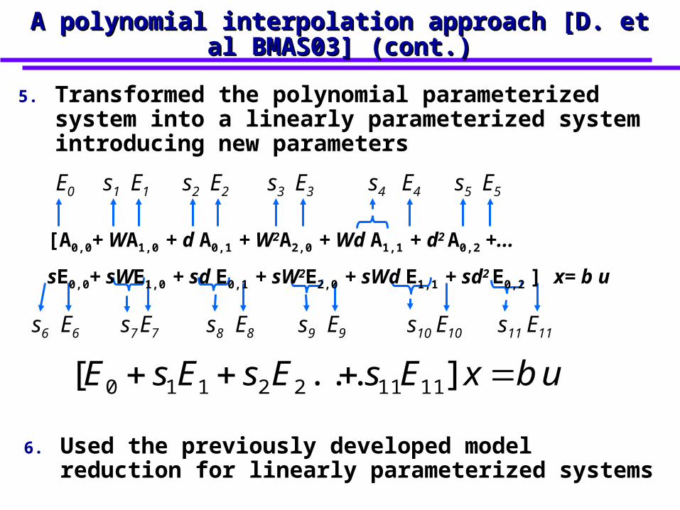
6. Used the previously developed model reduction for linearly parameterized systems

5. Transformed the polynomial parameterized system into a linearly parameterized system introducing new parameters

E0 E1 E2 E3 E4 E5

E11E10E9E8E7E6

s1 s2 s3 s4 s5

s11s10s9s8s7s6

[A0,0+ WA1,0 + d A0,1 + W2A2,0 + Wd A1,1 + d2 A0,2 +...

sE0,0+ sWE1,0 + sd E0,1 + sW2E2,0 + sWd E1,1 + sd2 E0,2 ] x= b u

ubxEsEsEsE ]...[ 111122110

45

More in general...More in general...[D. TCAD04] [D. PhD04][D. TCAD04] [D. PhD04]

ubxEsWdEWE 1,1,10,2,02

0,0,0 ......

21 2 1 1 2 2 1, , , , , , ,px span b E b E b E b E b E E E E b

ˆq xx U

Uq

It is a p-variables Taylor series expansion

buEsEsEsxm

mpp 2211

Once again change basis:Once again change basis: use first few vectors of the use first few vectors of the

Taylor expansion,Taylor expansion, matching first few matching first few

derivatives with respect to derivatives with respect to each parametereach parameter

46

Computational Complexity (time and memory)Computational Complexity (time and memory)

bEEbbUq2

Computational Complexity

Hankel reductionor Balance Realizations

O(N3)e.g. 10months for N=100,000

Moment matching O(q N2) e.g. 8days for N=100,000 q=10

Moment Matching + pFFT O(q N log N)e.g. 8hours for N=100,000 q=10

Moment matching bottleneck:

getting Eb, E2b, ...

47

pFFT: an O(NlogN) Matrix-Vector productpFFT: an O(NlogN) Matrix-Vector productfor the Mixed Potential Integral equations [Phillips97]for the Mixed Potential Integral equations [Phillips97]

Matrix-vector product Eb physical interpretation:

(1(1)) (2)(2)

(3)(3)

Picture by J. Phillips

(1) Project charges into a 3D grid. Complexity O(N)

(2) Calculate grid potentials, it is a convolution use FFT. Complexity O(n log n).

(3) Interpolate potentials from grid. Complexity O(N)

given N charges on N panels calculate the resulting N

potentials

grid points n ≈ N panels

48

PEEC Discretization Example: PEEC Discretization Example: On-Chip RF Inductor [D. BMAS03]On-Chip RF Inductor [D. BMAS03]

x100um

x100um

wire separation d = 1um-5umwire width W = 1um-5um

overall dimensions = 600um x 600umwire thickness 1um

picture not to scale

W

d

Results: Inductance vs. frequencyResults: Inductance vs. frequency

frequency [ x10GHz ]

Wire width = 5umseparation = 1um, 2um, 3um, 4um, 5um



L L__ original system (order 420)--- reduced model (order 12)

__ original system (order 420)--- reduced model (order 12)

Worst case errorin resonance position = 3%

Results: Quality factor (Q=wL/R) vs. frequencyResults: Quality factor (Q=wL/R) vs. frequency



frequency [ x10GHz ]frequency [ x10GHz ]

Worst case errorin amplitude = 4%



Q Q

51

Open issues Open issues in the PMOR Matrix Reduction stepin the PMOR Matrix Reduction step

Model order grows as O(pm) where p = # parameters and m = # derivatives matched for each parameter however model order is linear in # of parameters when

matching only one derivative per parameter (m = 1) and still produces good accuracy in our experiments.

furthermore, for higher accuracy instead of increasing # of matched derivatives, can instead match multiple points (or combine the two approaches) [Li, Liu, Nassif, Pileggi DATE05]

W or d

Limitations and future workLimitations and future workuse better interpolation!use better interpolation!




Q

very little error in thepoints used for fitting1um, 3um, 5um

Worst case errors far from fitting points 2um, 4um (3% in resonance position)

so the critical stepis the fitting!!

Case #2. The parameter is frequency.Case #2. The parameter is frequency.Already discussed: Distributed Linear Systems Already discussed: Distributed Linear Systems

Examples: full-wave MPIE MPIE using layered-media Green functions (e.g. for

handling substrate or dielectrics) frequency-dependent basis functions frequency dependent discretizations

xcy

buxsssET

p

),,,( 1

Polinomial interpolation for frequency Polinomial interpolation for frequency [Phillips96][Phillips96]

Polynomial approximation e.g. Taylor expansion, or a polynomial interpolation for E(s)

Performance: Fast and accurate in the frequency band of interest

Problem: Can not be used in a time domain circuit simulator because does not guarantee stability and passivity

buxEsEssEE MM 2

210

xcybuxsE T)(

Positive real transfer functionPositive real transfer functionin the complex plane for different frequenciesin the complex plane for different frequencies

)}(Re{ jH

sfrequencie allfor ,0)}(Re{ jHPassive regionActive

region

)}(Im{ jH

original system )( jH

Why does polynomial interpolation failWhy does polynomial interpolation failwhen applied to the Laplace parameter ‘s’?when applied to the Laplace parameter ‘s’?

original system )( jH

)}(Im{ jH

Passive regionActiveregion

Although accurate in the frequency band of interest

Polynomial interpolation is unlikely to preserve GLOBAL properties such as positive realness because it is GLOBALLY not well-behaved

)}(Re{ jH

sfrequencie allfor ,0)}(Re{ jH

Using global uniformly convergent interpolantsUsing global uniformly convergent interpolants[Daniel02][Daniel02]

If E(s) is strictly positive real, a GLOBALLY and UNIFORMLY convergent interpolant will eventually get close enough (for a large enough order M of the interpolant) and be positive-real as well.

Re

Imoriginal system )( jE

reduced system )(ˆ jE

Proof: just choose

accuracy of interpolation smaller than minimum distance from imaginary axis

M

kkk

M sEsE0

)( )()(

sfrequencie allfor ,0)}(Re{ jEPassive regionActive

region

Parameterized reduction can enable automatic design of circuit components that can only be described by field solvers

All methods presented are based on Krylov subspace moment matching projection

Key observation: all these methods are compatible with O(NlogN) field solver based matrix-vector

But of course all these methods also have all the arguable issues associated with moment matching

Linearly parameterized (use p-variable Taylor series expansion e.g. interconnect bus

Non-linearly parameterized (use polynomial interpolation) e.g. RF inductor (no substrate)

Distributed systems i.e. non-linear in s (use globally convergent interpolant implemented with FFT) e.g. substrate layered green functions or high order basis

functions

ConclusionsConclusions

59





Moment Matching with NON-linear parametersExample utilization of PMOR



Accelerated Optical Topography Using

Parameterized Model Order Reduction

Junghoon Lee, Dimitry Vasilyev, Anne Vithayathil, Luca Daniel, and Jacob White

Research Laboratory of Electronics

Massachusetts Institute of Technology

http://www.rle.mit.edu/cpg

TH3D-3

Non-destructive Inspection of Fabricated Structures• Spectroscopic ellipsometry

– Shine light of =200~800nm– Measure the scattered light– Estimate the geometric parameters, e.g. w and h

plasma-processing.com/insitu.htm www.sopra-sa.com

etched structure scattered field measurements

Model Based Approach

• Determine parameters p by solving

• Solve nonlinear least squares problem– Algorithms are iterative in nature– Scattering model evaluated for many p’s

• Need an efficient model of parameters p– Up to a dozen parameters– width (w), height (h), left/right sidewall angle, top

curvature, etc.

Model Possibilities

• Tabulated library of scattered fields

– Table grows exponentially as the number of parameters grow

• Full EM simulation for scattered field

– Too computationally expensive (too slow)

• New approach: automatic extraction of parameterized low-order model

– Automatically extract parameterized low-order model from pre-determined test structures

– Use model in optimization during in-line process diagnosis

Surface Integral Formulation

• Discretized surface integral formulation– PMCHW formulation on dielectric interfaces– Discretization and RWG basis functions– Method of moments

• Resulting system of equations

scattered field

integral ofincident wave

weights for RWG basis

discretizedintegral operators

• Polynomial fitting to find explicit dependency– y(p;): rough function of p and – A(p;), C(p;): smooth function of p and

• Polynomial fit of A and C

• Accurate since they are smooth

Polynomial Fitting

coefficient matrices

Parameterized Moment Matching

• Projection representation: approximate xf as

• Many different ways to choose V– Moment matching, balanced realization, POD, etc.– We used moment matching: match Taylor

coefficients of yf(p;) and yi(p;)

Parameterized Moment Matching

• Fitting with moment matching: for the constant

term

• Overall reduced system

Accelerated Optimization with Reduced Model

err

or

radius

original: 576

reduced: 30

(about x8000 faster)

err

or

width

True: 97 nm

Predicted: 97.3 nm

original: 540

reduced: 50

(about x1000 faster)

True: 105 nm

Predicted: 104.9 nm

Conclusions

• Optical Inspection Problem:

– Parameterized reduced model using polynomial fitting plus projection

– Accelerates optimization– The method achieves good accuracy in practice

• Acknowledgements

MARCO designated Interconnect Focus Centers,

SRC, Singapore-MIT Alliance, and NSF

70








A Quasi-Convex Optimization Approach to Parameterized Model Order Reduction

Linear analog componentse.g. interconnect, packages, RF inductors

Field Solver Linear Models

Parameterized Reduced Linear Models),(

),(),(),(reduced pea

pejcpebpH

j

jj

)()()( tuBtxpAdt

dx

Review: Quasi-Convex setupfor NON-parameterized MOR

, ,

( )minimize ( )

( )

deg , deg

deg ,subject to

0, [0, ]

0, [0, ]

j j

jja b c

j

j

b e jc eH e

a e

a m b m

c m

a e

b e

convex setStability:

Passivity:

quasi-convex set

Standard problem.Use for example by the ellipsoid algorithm

Parameterized MOR setup

• Let design parameter p explicitly enter (a,b,c)

1 11 0

1 11 0

111

,

,

,

m m m mm m

m m m mm m

m mmj

p p p pa a z a z z a z z a

b b z b z z b z z b

c c z c z z

p p

c z z

p p

p p p

• More difficult to check stability

• Construct guaranteed stable parameterized reduced model

Parameterized stability• Need to check a(z,p) > 0 for all z, for all p• Cannot use the trick in the non-parameterized case• Make a(z,p) a multivariate trigonometric polynomial

• Check positivity of multivariate trigonometric polynomial by using sum-of-squares argument

ˆ, , ,p pa z p a z p z a z z

trig poly ordinary poly trig poly trig polys

11 12 4p p pp z p p p p z z with

Positivity of multivariate trig. polyGiven a(z,p), solving the semi-definite program

,min

subject to W ,

0

y W W

p

y

y a z z

W

*, W W 0pa z z y

• Otherwise, claim a(z,p) 0 at some point

• If feasible and y* < 0, then

Example 7: Parameterized RF inductor

• Construct reduced order models in the design space

2 4 6 8 10 12 14 16 18 20

2

4

6

8

10

12

14

16

18

20

W (m)

D ( m

)

• Identify dominant poles z*(p)of each ROM

• Construct “non-dominant” systems such that

2 1

* *

( )ˆ ( , ) ( ) ( , )( ) ( )

K pG z p z A p z G z p

z z p z z p

where K(p), A(p) are scalars functionsG1(z,p) is the “non-dominant” system

• Construct parameterized ROM of each “non-dominant” system• Interpolate the scalars functions

• Combine both parameterized models to obtain the final model

Circle: training pointsTriangle: test points

Example 6: Parameterized RF inductor

2 4 6 8 10 12 14 16 18 20

2

4

6

8

10

12

14

16

18

20

W (m)

D ( m

)

Circle: training points

0 2 4 6 8 10 12

x 109

-5

0

5

10

15

20

25

30

35

40

frequency (Hz)

qual

ity f

acto

r

Quality factor for W=16.5 µm,D = 1,5,18,20 µm

Triangle: test points----- full model___ our QCO PMOR

Parameterized RF inductor (cont.)

0 2 4 6 8 10 12

x 109

-5

0

5

10

15

20

25

30

35

40

frequency (Hz)

qual

ity f

acto

r

0 2 4 6 8 10 12 14 16 18 202.5

3

3.5

4

4.5

5

5.5

6

6.5x 10

9

D ( m)

argm

ax(Q

) (H

z)

Quality factor for W=16.5 µm, D = 1,5,18,20 µm

Frequency of the peak Q factor for W = 16.5 µm

Summary of Quasi-Convex Optimization basedParameterized Model Order Reduction

• QCO competes reasonably well with existing alg (e.g. PRIMA) for reducing large systems

• But in addition: QCO can reduce models with frequency dependent matrices

• QCO is very flexible in imposing constraints such as stability and passivity

• QCO can be extended to parameterized MOR problems

80








81

““Field Solver Accurate” and AutomaticField Solver Accurate” and AutomaticParameterized Reduced Order Modeling Parameterized Reduced Order Modeling

of NonLinear Analog and MEMs of NonLinear Analog and MEMs ComponentsComponents

Luca Daniel, [email protected]

with contributions from Brad Bond

www.rle.mit.edu

mailto:[email protected]

82

Parameterized Model Order Reduction.Parameterized Model Order Reduction.ApplicationsApplications

interconnectRF inductors

matrix size

# parameters

linearity



Linear Time Invariant Non-Linear Systems

LOLNA ADC

MEMS

Packages

83

Case 3. Reduction of NonLinear SystemsCase 3. Reduction of NonLinear Systems

Non-Linear analog components

e.g. MEMs, VCO, LNA

)()),(( tuBptxFdt

dx

)(ˆ)),(ˆ(ˆˆtuBptxF

dt

xd

Parameterized NonLinear ReductionParameterized NonLinear Reduction

PDE Field Solvers or Circuit SimulatorsPDE Field Solvers or Circuit Simulators

Parameterized Model Order Reduction.Linear Systems

Moment Matching approaches - (Pullela97, Gunupudi00, Prud’homme02, Daniel02, Li05)

-Can handle nonlinear dependence on parameter

-Can handle extremely large systems

Optimization based approaches - (Sou05)

-Good for fitting data from measurements

-Cannot construct large order reduced models

Statistical Data Mining - (Liu02)

-Can handle nonlinear parameter dependence and nonlinear systems

-Does not work well for extremely large systems

Truncated Balance Realizations - (Heydari01, Phillips04)

- Does not handle extremely large systems

Previous work on Non-ParameterizedMOR for nonlinear systems

Representation of FRepresentation of F(x)(x) using using a polynomiala polynomial (e.g. Taylor’s (e.g. Taylor’s expansions, Volterra Series) [Phillips00]*****expansions, Volterra Series) [Phillips00]*****

Representation of F(x) using Representation of F(x) using several linearizationsseveral linearizations (Trajectory Piece-Wise Linear TPWL) [Rewienski01](Trajectory Piece-Wise Linear TPWL) [Rewienski01]

...)()(

)()(

00

00

xxxxW

xxAxFxF

...

)()()(

)()()(

22222

11111

xxAxFxw

xxAxFxwxF

)())(( tbutxFdt

dxE

Representation of F(x) with Representation of F(x) with several polynomialsseveral polynomials (PWP (PWP PieceWise Polynomial) [Dong03]PieceWise Polynomial) [Dong03]

k

iiii tbuKtxAxw

dt

dxE

1

)()( 00 tbuKtxAdt

dxE

x3x1

x7x6x5

Use collection of linear models

Background – TPWL [Reiwenski01]

x1

x2

x10x8

x4

x2

x14

x15

13J

xa

xb

x0

0J

bJ

aJ

x11x9

3J2J1J

4J 5J6J 7J

8J 9J 10J 11J x13

14J

15J#linearizations =#samples#linearizations =#samplesnn

n = 10n = 1044 #samples = 100#samples = 100

1001001000010000 = LARGE = LARGE

Model i only valid near xi

Background – TPWL: Picking Linearization Points

x1

x2

t

y(t)

Use training trajectories to pick linearization points

Error

Linearization at current state xi

State SpaceTime Domain Simulation

Background – TPWL: Weighting / Simulation[Riewinski01,Tiwary05,Dong05]

Use weighting functions to combine linear models during simulation

x1

x2

tbuKtxAwKtxAwKtxAwdt

dxE 333222111

tbuKtxAKtxAKtxAdt

dxE 332211 001

tbuKtxAKtxAKtxAdt

dxE 332211 05.05.0

tbuKtxAKtxAKtxAdt

dxE 332211 3.06.01.0

0tt

1tt 2tt

3tt

tbuKtxAKtxAKtxAdt

dxE 332211 9.01.00

Current state

Linearization 3

Linearization 2

Linearization 1

C – poorlyapproximated

also wellapproximated Well approximated

89

Background – TPWLBackground – TPWLReduction of the Linearized SystemsReduction of the Linearized Systems

dt

dxE tbu

Model from linearization 1

A1A1 K1K1x1w 2w kw

Model from linearization 2

A2A2 K2K2x

Model from linearization k

AkAk KkKkx

dt

xdE

ˆˆ1A 2A kA

1K 2KkK

tub x x x1w2w kw

=UTU

iA iA

90

Background – TPWLBackground – TPWLConstructing the projection matrix VConstructing the projection matrix V

Use moments from EACH linear model to construct V

bMbMbMbMbMbspanx qk

q ,,,,,,, 212

11

bMbMbMbMbU qk

q ~~~~~ 1211

=UTU

iA iA

Outline

• Introduction• Background

• NonLinear Parameterized Model Order Reduction (NLPMOR)– Constructing the system– How to pick linearization points– How to construct V

• Examples• Results• Conclusions• Future Work

NLPMOR – Constructing the System

Start with system possessing nonlinear dependence on state x and parameters sj

tbusstxFdt

dxE ,...,, 1

p

jjj tbutxFs

dt

dxE

0

~~

k

i

p

jijijji tbuKtxAsxw

dt

dxE

1 0

~~~

Obtain Linear dependence on new parameters

Linearize to get weighted sum of

linear models

By linear approximation, polynomial fitting to data points…

Single linear model

Weighting basis functions

js~

1~0 s

Non-Linear Parameterized Reduction[Bond, Daniel ICCAD05]

x1

x2

time

y(t)

Use training trajectories to pick linearization points

s1

s2

1s

2sTrain again at different points in parameter space

Parameter Space

Repeat at different points in parameter space to populate state space

State Space

Non-Linear Parameterized Reduction[Bond, Daniel ICCAD05]

1s

2s

4s

5s 3s

Populate relevant regions of state-space with linear models from training at different inputs or different points in parameter-space

Parameter Space

s2

s1

x1

x2

State Space

NLPMOR – Constructing V: 2 Options

,~

,~

,~

,,~

,~

,~

,~

,~

,,~

,~

,~

,~

,~

,,~

,~

,~

01102010

220212120222022221220

11011111012

10111111101

kkkkkkkkkpkkkk

p

p

bMMMMbMbMbMbM

bMMMMbMbMbMbM

bMMMMbMbMbMbMb

spanx

ijiij AAM~~ 1

0

kqk

q bMbMbMbMbMbspanx~

,,~

,~

,,~

,~

,~

221112

1111

EAsMp

jijji

1

0

~~

Single variable Taylor series expansion of x for each model, as in TPWL

p-variable Taylor series expansion of x as in PMOR, but for each model

OR

V

V

“PMOR V”

“MOR V”

Option 1

Option 2

bAsb ij

p

jji

1

0

~~~

EAM ii1

00

~ bAb ii1

0

~~

96

Non-Linear Parameterized ReductionConstructing V

For qth order model with p parameters and k linear models, total number of vectors for V is O(kpm)

Keeping all vectors would results in a huge “reduced” model

Hence we perform an SVD on V and keep only the q most important vectors

SVD

NN

O(kpm) q

V V

NLPMOR – 4 Algorithms

p

jjj tbutxFs

dt

dxE

0

~~

k

i

p

jijijji tbuKtxAsxw

dt

dxE

1 0

~~~ tbusstxFdt

dxE ,...,, 1

Train at single p-space point

Train at multiple p-space points

k

i

p

jijijji tubKtxAsxw

dt

xdE

1 0

ˆ~ˆ

~~ˆˆˆˆ

Linearize in parameters sj

Original Model

Train to pick linearization points xi

MOR

V

PMOR

V

MOR

V

PMOR

V

Parameter Space

x xV x xVMOR

PMOR

TPWL ALG1 ALG2 ALG3

Single p-space point training

Multiple p-space point training

MOR V

PMOR V

TPWL ALG2

ALG1 ALG3

Outline

• Introduction• Background• NLPMOR

• Examples–Circuit–Beam

• Results• Conclusions• Future Work

Analog Circuit Example

Nonlinear terms

Analog circuit with nonlinear components distributed throughoutUsing constitutive relations for each element, apply KCL at each node to obtain state-space model

cidt

dVC

1exp

Tdd v

VIVi

r

Vir

Picture by Michał Rewienski

Analog Circuit Example – State Space System

tbutxDtGxdt

tdxE

State-Space System

11

11

11 jjjj xxxx

djjjjj eeIxx

rxx

rdt

dxC

Resistor values

Turn on voltageSaturation currentCapacitor values

Possible parameters

Single equation at node j

Analog Circuit Example – One possible parameterized model

tbuKxAKxAwdt

dxE

k

iiiiii

11100

Selected parameter: α Obtained linear dependence on parameters

Time (s)

Vo

ltag

e (V

)

Full Model

ALG1 ROM

0 002.1

Training point

Evaluation point

Single point training

Multiple point training

MOR V

PMOR V

ALG1

Micromachined Switch Example

t

pzppzK

t

zhwdypp

z

wv

x

zhwS

x

zwhEI

w

a

1261

2

3

2

2

0

02

20

2

2

04

43

0

Governing Equations

DiscretizePicture by Michał Rewienski

Micromachined Switch ExampleState Space System

State-Space System

3331

1131

323

2

0

041

43

021

2

0

0

30

31

31

222

31

21

6112

1

3

2

33

3

2

3

xxxxxx

xx

dt

dx

vhx

xwhEI

x

xhwSdypx

hw

x

x

x

dt

dx

x

x

dt

dx

w

a

Beam width

Material Properties

Beam height

Possible Parameters

Micromachined Switch ExampleOne possible parameterized model

)(11001 3

2

1

3

2

13

2

1

tbuKAKAwdt

d

ixxx

iixxx

i

k

ii

xxx

u(t) = 5.52 , t > 0 Full Model

ALG2 ROM

01 072.0

Training point

Evaluation point

02

Single training

Multiple training

MOR V

PMOR V

ALG2

System parameterized inw

1

Outline

• Introduction• Background• NLPMOR• Examples

• Results–Algorithm Comparison–Algorithm Cost

• Conclusions• Future Work

Analog Circuit Example – Algorithm 1

dI

R

1

1

0.9

1.4

1e-10 1.5e-100.5e-10

Full Model

ALG1 ROM

- Training points

- Evaluation points

Single training

Multiple training

MOR V

PMOR V

ALG1

Results – Benefit of PMOR V

Id0

Accuracy

Id

TPWL – MOR V

ALG1 – PMOR V

Trained at Id0



MOR V

PMOR V

TPWL

ALG1

Err

or

TPWL

ALG1

IdId0

Analog Circuit

Analog Circuit TPWL ROM

ALG1 ROM

Analog Circuit Example

dI

R

1

1

0.5

1.5

1e-10 1.5e-100.5e-10

This model is parameterized in Id and 1/R, and was created using ALG2

2

2e-10

- Training points

- Evaluation points

Full Model

ALG2 ROM

Single training

Multiple training

MOR V

PMOR V

ALG2

Results – Benefit of multiple training points in p-space



MOR V

PMOR V

TPWL ALG2

Id0

Accuracy

Id

TPWL – trained at Id0

ALG2 – trained at Id1, Id2

Id2Id1

Id1 Id2Id0

% E

rror

TPWL

ALG2

% E

rror

time (s)

MEMs Switch

TPWL ROM

ALG2 ROM

Analog Circuit

Results – Algorithm Comparisons

Each algorithm covers a different region of p-space

Parameter Space Validity of Models

S1

S2

s2A

s1A s1B

s2B

All algorithms produce model with same reduced order and same number of linear pieces



MOR V

PMOR V

TPWL ALG2

ALG1 ALG3

Results – Algorithm Comparisons

Each algorithm has a different cost

AlgorithmCost of

constructing V(in system solves)

Training cost(trajectories made

per input)

TPWL

ALG 1

ALG 2

ALG 3

O(km)

O(kpm)

O(krpm)

O(krppm)

1

rp

rp

1

Majority of cost lies in training

Majority of cost lies in making vectors for V

Expensive in both training and creating V

Cheap

p - # of parameters k - # of linear models per trajectoryr - # of parameter values usedm - # of moments matched per parameter



MOR V

PMOR V

TPWL ALG2

ALG1 ALG3

Conclusions

• NLPMOR– Captures nonlinear effects

– Preserves parameter dependence

• Algorithm choice is situation/system dependent– TPWL, ALG1 can provide high accuracy locally in

parameter space

– ALG2, ALG3 can provide global accuracy in parameter space

– ALG1, ALG3 : expensive to create V

– ALG2, ALG3 : expensive to train



MOR V

PMOR V

TPWL ALG2

ALG1 ALG3

Future Work in Parameterized Model Order Reduction of Non-Linear Systems

• Ensure stability and passivity of Non-Linear reduced order models

• Try other approaches for Projection Matrix – e.g. TBR, Quasi-Convex Optimization

• Try other approaches for capturing nonlinearity– e.g. Volterra series, or piece-wise polynomial

Summary of the courseSummary of the course

Model Order Reduction of Linear SystemsKrylov + TBR two step procedure

1st step: Krylov Moment Matching Projection PVL or PRIMA (for passive systems)

2nd step Truncated Balance Realization (TBR) or Passive-TRBDistributed Passive Systems:

Quasi Convex OptimizationLaguerre interpolation

Model Order Reduction of NonLinear SystemsWeakly Nonlinear: use Volterra series + moment matchingStrongly Nonlinear: use TPWL + moment matching (and/or TBR)

Parameterized Model Order Reduction Linear: moment matching OR quasi-convex optimization NonLinear: TWPL + moment matching