recent advances in atmospheric, solar-terrestrial physics...
TRANSCRIPT

21
Recent Advances in Atmospheric, Solar-Terrestrial Physics and Space Weather
From a North-South network of scientists [2006-2016]"
PART B : Results and Capacity Building
Amory-Mazaudier, C. 1,2, Fleury, R. 3, Petitdidier, M.4 , Soula, S.5, Masson, F.6, GIRGEA team1*, Davila, J.7, Doherty, P.8, Elias, A.G.9, Gadimova, S.10,Makela, J.11, Nava, B.2,
Radicella, S.2, Richardson, J.12, Touzani, A.13 1. Sorbonne Universités UPMC Paris 06, LPP, Polytechnique, Paris, France
2. T/ICT4D Abdus Salam ICTP, Trieste, Italy 3. Lab-STICC, UMR 6285, Institut Mines-Telecom Atlantique, Brest cédex 3, France
4. Université Versailles Saint-Quentin, CNRS/INSU, LATMOS, IPSL, Guyancourt, France 5. Laboratoire d’Aérologie, Université de Toulouse, France
6. Institut de Physique du globe de Strasbourg, Ecole et Observatoire des Sciences de la Terre, 5 rue Réné Descartes, 67084, Strasbourg Cédéx, France
7. NASA, Independence Square at 300 E, Street SW, Washington D.C., USA 8. Boston College University, Boston, USA
9. Conicet & Universidad Nacional de Tucuman, Departamento de Fisica, Tucuman, Argentina
10. Office for Outer Space Affairs, United Nations Office at Vienna 11. Department of Electrical and Computer Engineering, University of Illinois at Urbana-
Champaign, Urbana, Illinois, USA 12. Massachusetts Institute of technology, Kavli Institute for Astrophysics and Space
Research, Cambridge, MA 13. African Regional Centre for Space Science and Technology Education (CRASTE-LF)
E mail ([email protected]).
Accepted : 22 September 2017
Abstract This paper reviews scientific advances achieved by a North-South network between 2006 and 2016. These scientific advances concern solar terrestrial physics, atmospheric physics and space weather. This part B is devoted to the results and capacity building. Our network began in 1991, in solar terrestrial physics, by our participation in the two projects: International Equatorial Electrojet Year IEEY [1992-1993] and International Heliophysical Year IHY [2007-2009]. These two projects were mainly focused on the equatorial ionosphere in Africa. In Atmospheric physics our research focused on gravity waves in the framework of the African Multidisciplinary Monsoon Analysis project n°1 [2005-2009 ], on hydrology in the Congo river basin and on lightning in Central Africa, the most lightning part of the world. In Vietnam the study of a broad climate data base highlighted global warming. In space weather, our results essentially concern the impact of solar events on global navigation satellite system GNSS and on the effects of solar events on the circulation of electric currents in the earth (GIC). This research began in the framework of the international space weather initiative project ISWI [2010-2012]. Finally, all these scientific projects have enabled young scientists from the South to publish original results and to obtain positions in their countries. These projects have also crossed disciplinary boundaries and defined a more diversified education which led to the training of specialists in a specific field with knowledge of related scientific fields. © 2017 BBSCS RN SWS. All rights reserved
Keywords: Space weather, Equatorial Electrojet Year (IEEY), International Heliophysical Year (IHY), international space weather initiative project (ISWI)
1 See page 24

Amory-Mazaudier C. et.al. Recent Advances in Atmospheric, Solar-… PART B : Results and Capacity Building
22
TABLE OF CONTENTS
1: Atmospheric Physics 25 Introduction
1.1 Climate 25 1.1.1 Sunshine and cloudiness 1.1.2 Solar activity and meteorological fluctuations in West Africa: Temperatures and
Pluviometry in Burkina Faso, 1970-2012 1.2 Onset of the Summer Monsoon over the southern Vietnam and its predictability:
determination of onset dates 26 1.3 Climatology of low-stratosphere gravity waves during the West African Monsoon 27 1.4 Atmospheric electricity in Central Africa 27 1.5 Hydrology of organic matter in the Congo Basin 29 1.6 Climatology of thermospheric winds over the eastern part of North Africa. 29
Concluding remarks
2: Solar terrestrial Physics 31 Introduction
2.1 Data, method and models used in this section 31 2.1.1 Data and method
2.1.1a Ionosonde
2.1.1b GNSS
2.1.1c Magnetic data/magnetometers
2.1.1d Method used to analyze magnetic data: 2.1.2 Models
2.1.2a GIM / CODG model
2.1.2b IRI: International Reference model
2.1.2c NeQuick model
2.1.2d TIEGCM model 2.2 Sun, Solar activity, solar wind, aurora activity and geomagnetism 33
2.2.1 Sun 2.2.2 Long term variations of the magnetic activity (>150 years) and signatures of events 2.2.3 Long term variation of the solar wind
2.3 Regular variations of the ionization and comparison with models 34 2.3.1 Regular variations of the ionization
2.3.1a Diurnal,
2.3.1b Seasonal, solar cycle 2.3.2 Comparison with models
2.3.2a Comparison with IRI model
2.3.2b Comparison with CODG model
2.3.2c Comparison with NeQuick and CODG models
2.3.2d Comparison with TIE-GCM model 2.3.3 Long term variations
2.4 Irregular variations of the ionization and comparison with models 40 2.4.1 Statistical studies 2.4.2 Case studies
2.5 Geomagnetism Sq, EEJ 42 2.5.1 Regular variations Sq EEJ 2.5.2 Sq and stratospheric warming
2.6 Electrodynamics parameters 44 2.6.1 Ionosphere Conductivity model 2.6.2 ExB Drift 2.6.3 Electric current densities
2.7 The equivalent electric current systems 46 2.7.1 DP2 and Ddyn
2.7.1a DP2
2.7.1b Ddyn 2.7.2 Hemispheric Asymmetry
2.8 Electromagnetic induction studies in the presence of EEJ 49 2.9 Ion density [O +] from DEMETER satellite 50
Concluding remarks

Sun and Geosphere, 2017; 12/ 2-Supplement 21÷69 ISSN 2367-8852
23
3. Space weather 52 Introduction
3.1 Definitions of the main disturbances and indices 52 3.1.2 Spread F 3.1.2 ROTI index
3.2 Detection of SC 53 3.3 Flare effect 53 3.4 Geomagnetic storms: Wavelet-based multiscale analysis of geomagnetic disturbance 53 3.5 Impact on GNSS: case studies 53
3.5.1 CME + high speed solar wind 3.5.2 Series of CME with + high speed solar wind
3.6 GIC: Induced effects of the solar flare of 04 April, 1993 56 3.7 Spread F/HF and Scintillations /GNSS 59
3.7.1 The Spread-F observed at Phu Thuy, Vietnam 3.7.2 Scintillations observed at Kinshasa
Concluding remarks
4. Capacity building and societal development 60 Introduction
4.1 Training and international projects 60 4.2 Cursus 61
4.2.1. Training on the Solar terrestrial physics in an integrated framework 4.2.2. Analysis and processing of GNSS data for the different disciplines
4.3 GNSS development in DRC 61 4.4 Satellite-Based Augmentation System (SBAS) 63
Concluding remarks
General Conclusion 63
References 64

Amory-Mazaudier C. et.al. Recent Advances in Atmospheric, Solar-… PART B : Results and Capacity Building
24
GIRGEA team * Menvielle M.1, Damé L.1, Berthelier J-J.1, Georgis L.2, Philippon N.3, Adohi J-P.4, Anad F.5, Bolaji O.6,7, Boka K.4, Bouhnir A.8, Chane-Ming F.9, Curto J-J.10, Dinga B.11, Doumbia V.4, Fathy I.12, Gaye I.13, Kafando P.14, Kahindo B.15, Kazadi A.15, Kobéa A.T.4, Le Huy M.16, Le Truong T.16, Luu Viet H.17, Mahrous A.12, Mbane C.18, Nguyen Chien T.16, Niangoran M.19, Obrou O.4, Ouattara F.20, Pham Thi Thu H.16, Pham Xuan T.16, Rabiu B.21, Shimeis A.22, Tran Thi L.16, Zaka K.Z.4, Zaourar N.23, Zerbo J-L.24
1. Université Versailles Saint-Quentin, CNRS/INSU, LATMOS, IPSL, Guyancourt, France
2. Laboratoire d’Aérologie, Université de Toulouse, France 3. Institut des Géosciences, Université Grenoble Alpes, Grenoble, France 4. Laboratoire de Physique de l’Atmosphère, Uni. Felix Houphouet Boigny, Abidjan, Côte d’ivoire. 5. CRAAG, BP 63 Bouzareah, Alger, Algérie 6. Department of Physics, University of Lagos, Nigeria 7. Department of Physics, University of Tasmania, Australia 8. Oukaimeden Observatory, Laboratoire de physique des hautes énergies et astrophysique FSSM,
Cadi Ayyad University, Marrakech, Morocco 9. Uni. de la Réunion, Lab. de l’Atmosphère et des Cyclones, UMR 8105, CNRS-Météo France-Uni.,
La Réunion, France 10. Observatorio del Ebro, (OE) CSIC – Universitat Ramon Llull, Roquetes, Spain 11. Université Marien Ngouabi, Brazzaville RC 12. Space Weather Monitoring Center, Faculty of Science, Helwan University, Helwan, Egypt. 13. Département informatique UFR SET, Université de Thies, Sénégal 14. Uni. Ouaga 1, Lab. de Physique et de Chimie de l’Environnement Ouagadougou, Burkina Faso 15. Université de Kinshasa, Kinshasa, RDC 16. Institute of Geophysics, Vietnam Academy of Science and Technology, Hanoi, Vietnam. 17. Ho Chi Minh city University of Technology and Education, Vietnam 18. University of Douala, Douala Cameroon 19. Université de Korhogo, Côte d’Ivoire 20. Université de Koudougou, Koudougou, Burkina Faso 21. Centre for Atmospheric Research, National Space Research and Development Agency,
Anyigba, Nigeria. 22. National Research Institute for Astronomy and Geophysics, Helwan, Egypt 23. Université des Sciences et de la Technologie Houari Boumediene, BP32 USTHB, 16123 Bab-
Ezzouar, Alger, Algérie, 24. Université Polytechnique de Bobo-Dioulasso, 01 BP 1091 Bobo-Dioulasso, Burkina Faso

Sun and Geosphere, 2017; 12/ 2-Supplement 21÷69 ISSN 2367-8852
25
Introduction This paper presents the results obtained by a North-South research network. This network was constituted and structured within
the framework of international projects based on the deployment of measurement instruments in non-equipped countries and particularly in Africa. A first part A is devoted to some aspects of the Sun Earth’s system useful to understand the results concerning the solar terrestrial physics and the space weather. This second part B presents the recent advances in Atmospheric, Solar-Terrestrial Physics and Space Weather.
It consists of 4 sections. The first section brings together results on climate and atmospheric sciences, in particular the monsoon in West Africa and Vietnam/Asia, lightning in the DRC, hydrology in the RC and upper atmospheric winds in Morocco. For each study discussed in the climate and atmospheric sciences section, we recall previous work so that the reader understands the scope of the results.The second section presents results mainly concerning the solar wind, geomagnetism and the ionosphere of low latitudes. The third section is devoted to space weather and focuses on the impacts of solar events (Solar Flare, Coronal Mass Ejection and High Speed Solar Wind) on variations in ionization and changes in the Earth's magnetic field. The fourth section presents the societal interests of our studies, in particular those concerning GNSS and the perspectives.
1 : Atmospheric Physics
Introduction Atmospheric Observations and their interpretation are very dependent on latitude, longitude, altitude, and time at different scales.
During years, some places over the world, like in Africa, Asia… were lacking from observations and scientists were obliged to imagine or interpolate what happen in those areas to carry out modelling. The first important event in atmospheric science to fill this gap was the International Geophysical Year (IGY) in 1957 by carrying observations all over the world, building a large data base published into books, disseminating knowledge and facilitating inter-exchange among teams. Since, many other topical years like EEY, EGY, IHY, AMMA… provide other opportunities to pursue observations all over the world, and studies via the large databases such created. The examples, given below, are related both to climatic phenomena based on the study of large databases in relation to solar data (Spain and Burkina Faso), as well as to regional phenomena such as the monsoon in Vietnam, the gravity waves related to the African monsoon in West Africa, the lightning in the DRC, the hydrology of the Congo River and the upper atmospheric winds in Morocco. It looks like a patchwork of individual studies; not so as a matter of fact they are well embedded into local, regional and international frameworks and then African, Asian scientists are becoming major actors of the knowledge development about atmospheric phenomena and climatology, essential for life in their countries.
1.1 Climate The Sun’s impact on our planet’s climate has recently been a hotly debated topic in the context of climate change. De Wit et al.
(2015) summarized what we know nowadays about the mechanisms by which solar variability may impact climate variability. None of these mechanisms can adequately explain global warming observed since the 1950s. However, several of them do impact climate variability, in particular on a regional level.
Sunshine and cloudiness Clouds are one of the most difficult climate components to
parameterize, and a source of large uncertainties in global climate model predictions. Clouds have two simultaneous and opposite effects on the radiative balance of the planet. On average, the cooling effect of clouds dominates over the warming, but the net radiative effect strongly depends on the type and altitude of the clouds, with thin high cloud types having an overall warming effect. In addition to poor understanding of the role of clouds, there is also the lack of accurate long-term data. In this sense, synoptic cloud observations taken from ground observatories, are our only probes of cloud changes on time scales of centuries. Sunshine is a basic parameter used to evaluate the amount of sunlight delivered at the top of the atmosphere that is able to reach the ground. Sunshine records could be used as a proxy for clouds.
Sunshine and synoptic cloud observations, extending over almost a century, are available from the Ebro Observatory and were studied by Curto et al. (2009c). They found a strong decadal variability in the duration of bright sunshine hours since 1910 and a monotonic increase in synoptic cloud amount since the 1920s. They interpreted these results as a change in cloud type frequency. Both series after being detrended and normalized are presented in Figure 1. The year-to-year variability in both time series is highly correlated and is highly statistically significant, indicating a closely matched inter-annual variability.
Figure 1: Time series of the detrended and normalized total
sunshine hours and the inverse of cloud amount at Ebro Observatory 1910–2006. Although there is no direct correspondence between the long-term trend of sunshine and cloudiness series, for shorter time scales as here the year-to-year variability, both time series are highly correlated (r = 0 .83 , P _ 99 %) indicating that the removed long trends might have a different physical mechanism (Curto et al., 2009c)

Amory-Mazaudier C. et.al. Recent Advances in Atmospheric, Solar-… PART B : Results and Capacity Building
26
1.1.2 Solar activity and Meteorological fluctuations in West Africa: Temperatures and Pluviometry in
Burkina Faso, 1970-2012 Zerbo et al. (2013a) reviewed on the close link between the solar activity indices and the climatic parameters (temperature and
rain fall) over more than three solar cycles. An investigation during the period 1970-2012 shows amazing correlation according which the highest level of rain fall is correlated with the lowest sunspot number. Solar cycle minimum is characterized by important precipitation and decrease in temperature. Likewise highest temperature level is recorded during the decreasing phase of solar cycle with significant decrease of rain fall. We can assume that active solar is associated with weak incident cosmic ray consequently with low cloudiness which brings warming. Likewise, quiet solar is associated with important cloud cover and consequently bring important precipitations and chills terrestrial atmosphere.
1.2 Onset of the Summer Monsoon over the southern Vietnam and its predictability: determination
of onset dates In the tropics, monsoon corresponds to seasonal changes in
atmospheric <https://en.wikipedia.org/wiki/Atmosphere_of_Earth> circulation and precipitation associated with the asymmetric heating of land and sea. One important point is to determine the actual date of the monsoon onset because often there are precipitations during several days during the expected period and they stop. The actual onset dates are important for agriculture.
According to the point of view of the climatologists, the wet season over southern Vietnam takes place from May to October, while the dry season occurs from November to April (Pham and Phan, 1993; Pham Xuan T. et al., 2008). Figure 2 presents the 5-day running climatology of the regional rainfall index for the 26-year study period as a black thick line. Jointly, the climatology of the daily zonal wind above the South Vietnam (grid point located at 10-12.5°N, 105-107.5°E) is provided as a thin gray line. This diagram shows that the transition from the dry to the wet season from April to May is characterized by (1) a sudden increase of the daily rainfall from 3 mm.day -1 in April to about 7 mm.day -1 in May, and (2) changes in the zonal wind component from negative (easterlies) to positive (westerlies) values.
Table 1: The onset date of the summer monsoon over
southern Vietnam
The date of monsoon onset has been defined in various ways. Holland (1986) defined the onset of the Australian summer monsoon through changes of the prevailing winds. Some other authors have defined the onset by focusing on precipitation only, fixing some threshold values of precipitation rate (Tao and Chen, 1987; Matsumoto, 1997; Wang and Ho, 2002; Zhang et al., 2002). The combination of wind and precipitation or convection activity data has also been used (Lau and Yang, 1997; Qian and Lee, 2000; Ding and Yanju, 2001). Recently, the reversal of the meridional temperature gradient in the upper troposphere (200-500hPa) has been shown as an interesting signal of the monsoon onset (Li and Yanai, 1996; Mao et al., 2004).
In this paper Pham Xuan T. et al., (2010) the onset date is defined for the 26 available years of the reference period given that the following conditions are verified:
1) The daily amount of our rainfall index exceeds 5 mm.day-1 and these conditions persist for at least 5 days.
2) The daily mean of our zonal wind index exceeds 0.5 m/s. These 2 conditions allow determination of the first occurrence of monsoon rains within the monsoon flow regime and are
sufficient for depicting correctly the onset. The addition of a persistence criterion such as “ Within the consecutive 20 days, the number of the days with rainfall greater than 5 mm day exceeds 10 days” used by Zhang et al. (2002) does not change the onset dates except in 1989.
The onset dates as defined above are displayed for each year of the study period in Table 1. The earliest onset occurred in 1979 (April, the 19th) and the latest one in 1993 (June, the 9th). The mean date is the 12 of May with a standard deviation of 11.6 days. This is consistent with previous results obtained for the Indochina region: 1-15 May (Qian and Lee, 2000), 6-10 May (Wang and Ho, 2002), and 9 May (Zhang et al., 2002).
Figure 2 : Daily climatology (5-day running mean) of rainfall index
in mm/day (solid) and daily mean zonal wind component in m/s (dashed) during 1979-2004. (Pham Xuan et al., 2008)
Year Onset
date Year
Onset
date
1979 19 Apr 1993 9 Jun
1980 19 May 1994 3 May
1981 11 May 1995 3 May
1982 1 May 1996 1 May
1983 12 May 1997 4 May
1984 5 May 1998 25 May
1985 25 May 1999 23 Apr
1986 11 May 2000 2 May
1987 16 May 2001 13 May
1988 21 May 2002 14 May
1989 8 May 2003 4 May
1990 16 May 2004 10 May
1991 8 Jun mean 12 May
1992 7 May

Sun and Geosphere, 2017; 12/ 2-Supplement 21÷69 ISSN 2367-8852
27
1.3 Climatology of low-stratosphere gravity waves during the West African Monsoon In the equatorial and tropical regions, deep convection is an important source of atmospheric gravity-waves (GWs). They ensure
the coupling of the atmosphere circulation from the troposphere to the upper atmosphere and interact with the Quasi Biennal Oscillation (QBO), the tropical and equatorial stratospheric feature (Fritts and Alexander, 2003). Although much progress has been done in numerical weather prediction and global models during this last decade, the representation of non-orographic GW sources such as tropical multi-scale convection still remains unresolved today. In the framework of the Stratospheric Processes and their Role in Climate (SPARC) (Allen and Vincent, 1995), initiative and of GW representation into models, Kafando et al. (2008; 2015) carry out climatology of GWs in the lower stratosphere (LS) at heights of 19-23 km over West Africa. They also take advantage of datasets
gathered by the African Monsoon Multidisciplinary Analyses (AMMA) (Redelsperger et al., 2006) project based on
multiscale observations in order to improve our knowledge and understanding of the West African Monsoon (WAM). Spectral characteristics of stratospheric GWs are derived from high vertical resolution profiles of radiosondes during 2006. Radiosondes (RS) were launched at six stations in a latitude range between 4°N and 17°N and a longitude range between 20°W and 10°E.
The annual variations of wave energy densities above the 6 selected stations are correlated with the progression of the rain belt and the convection over West Africa from the Guinea Gulf to the Sahel and their return back to Guinea Gulf. Over the equatorial coastal zone, high values of wave activity are observed during March-June corresponding to quasi-zonally propagating mesoscale wave, a mixture of equatorial and inertia-GWs. Lower values are observed in September-October with characteristics of inertia-GWs. Over the tropical West Africa, the WAM is installed during July and August. Wave spectral parameters point out that the major wave contribution is inertia-GWs with vertical and horizontal scales of 1.4–2.2 km and 450–1100 km respectively. In the range of short vertical wavelengths, the major contributor of the total wave energy is the kinetic energy density, KE, which is revealed to be a good proxy of inertia-GWs over West Africa; PE presents no significant variation in the presence of those waves.
The climatology of wave energy densities is determined over 9 years, from January 2001 to December 2009 at Niamey, a tropical station and at Douala, an equatorial station. The dataset is extracted from the Wyoming upper-air database. Above Niamey (13.47°N; 2.16°E), the inter-annual variation exhibits a quasi-2 year modulation of total energy density maxima during the WAM period correlated to the phase change of the QBO. A common pattern with higher peak observed in July-August during the W-phase (descending westerly winds) and no common pattern but erratic contribution during the monsoon period with small values during the QBO E-phase (descending easterly wind) i.e. the waves being filtered or damped (figure 3). For the equatorial coastal area, such a quasi-2 year modulation is not observed. This climatology shows a QBO-like variation with an impact on the wave energy into the LS.
Today remote sensing technology revolutionizes the science of meteorology and climatology by producing high-resolution vertical profiles of dynamical parameters on a global scale.
Figure 3 : Monthly mean total energy density in the lower stratosphere (19-23 km) above Niamey at 1200 UTC. Solid line:
mean for even years (2002, 2004, 2006 and 2008); Dashed line: mean for odd years (2001, 2003, 2005 and 2007). Error bars indicate the standard deviation.
1.4 Atmospheric electricity in Central Africa Lightning is a process of electric discharge specific to thunderstorm systems (MacGorman and Rust, 1998). It arises from a series
of processes that occur within the thundercloud and it has effects in broad areas, either natural or related to human activities. It produces electromagnetic radiation in a wide range of frequencies that can be exploited for its detection and location in order to monitor thunderstorm development, frequency, movements and climatology. During the 1990s, ground based detection systems
allowed to determine these informations at country scale (Orville, 1994). More recently, the global climatology of lightning activity developed by Christian et al. (2003) and based on data recorded during five years (May 1995-March 2000) by the Optical Transient Detector (OTD) loaded on board the satellite MicroLab-1, space observations have shown that the
Amory-Mazaudier C. et.al. Recent Advances in Atmospheric, Solar-… PART B : Results and Capacity Building
28
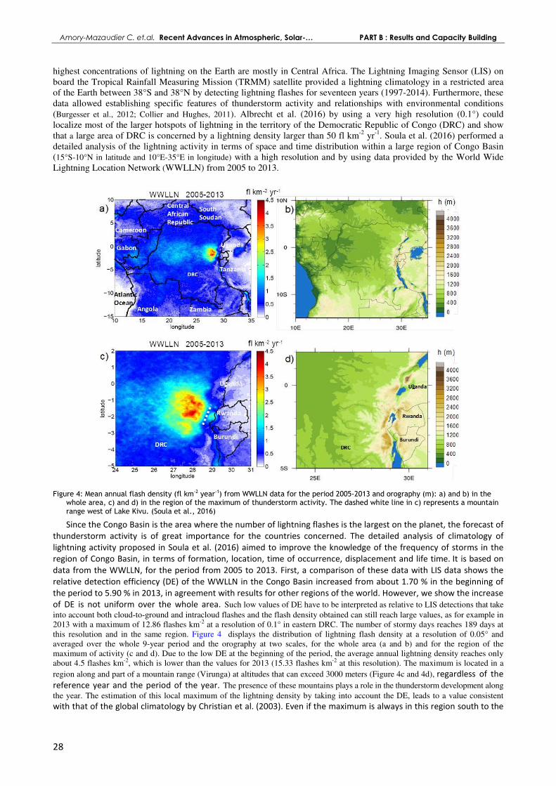
highest concentrations of lightning on the Earth are mostly in Central Africa. The Lightning Imaging Sensor (LIS) on board the Tropical Rainfall Measuring Mission (TRMM) satellite provided a lightning climatology in a restricted area of the Earth between 38°S and 38°N by detecting lightning flashes for seventeen years (1997-2014). Furthermore, these data allowed establishing specific features of thunderstorm activity and relationships with environmental conditions (Burgesser et al., 2012; Collier and Hughes, 2011). Albrecht et al. (2016) by using a very high resolution (0.1°) could localize most of the larger hotspots of lightning in the territory of the Democratic Republic of Congo (DRC) and show that a large area of DRC is concerned by a lightning density larger than 50 fl km-2 yr-1. Soula et al. (2016) performed a detailed analysis of the lightning activity in terms of space and time distribution within a large region of Congo Basin (15°S-10°N in latitude and 10°E-35°E in longitude) with a high resolution and by using data provided by the World Wide Lightning Location Network (WWLLN) from 2005 to 2013.
Figure 4: Mean annual flash density (fl km-2 year-1) from WWLLN data for the period 2005-2013 and orography (m): a) and b) in the
whole area, c) and d) in the region of the maximum of thunderstorm activity. The dashed white line in c) represents a mountain range west of Lake Kivu. (Soula et al., 2016)
Since the Congo Basin is the area where the number of lightning flashes is the largest on the planet, the forecast of
thunderstorm activity is of great importance for the countries concerned. The detailed analysis of climatology of
lightning activity proposed in Soula et al. (2016) aimed to improve the knowledge of the frequency of storms in the
region of Congo Basin, in terms of formation, location, time of occurrence, displacement and life time. It is based on
data from the WWLLN, for the period from 2005 to 2013. First, a comparison of these data with LIS data shows the
relative detection efficiency (DE) of the WWLLN in the Congo Basin increased from about 1.70 % in the beginning of
the period to 5.90 % in 2013, in agreement with results for other regions of the world. However, we show the increase
of DE is not uniform over the whole area. Such low values of DE have to be interpreted as relative to LIS detections that take
into account both cloud-to-ground and intracloud flashes and the flash density obtained can still reach large values, as for example in 2013 with a maximum of 12.86 flashes km-2 at a resolution of 0.1° in eastern DRC. The number of stormy days reaches 189 days at this resolution and in the same region. Figure 4 displays the distribution of lightning flash density at a resolution of 0.05° and averaged over the whole 9-year period and the orography at two scales, for the whole area (a and b) and for the region of the maximum of activity (c and d). Due to the low DE at the beginning of the period, the average annual lightning density reaches only about 4.5 flashes km-2, which is lower than the values for 2013 (15.33 flashes km-2 at this resolution). The maximum is located in a
region along and part of a mountain range (Virunga) at altitudes that can exceed 3000 meters (Figure 4c and 4d), regardless of the
reference year and the period of the year. The presence of these mountains plays a role in the thunderstorm development along
the year. The estimation of this local maximum of the lightning density by taking into account the DE, leads to a value consistent
with that of the global climatology by Christian et al. (2003). Even if the maximum is always in this region south to the

Sun and Geosphere, 2017; 12/ 2-Supplement 21÷69 ISSN 2367-8852
29
equator, the lightning activity seems to follow the sun displacement above the study area. However, the distribution of the flashes is
not symmetrical on both sides of the equator as indicated by the plot of the lightning density (Figure 4a), and a proportion of 66.67 %
is located in the southern hemisphere while only 60 % of the area is. Most of lakes correspond to an increase of the lightning
density, as for example Lake Victoria (33°E; 1°S), Lake Kivu (29°E; 2°S), Lake Tanganyka (29.5°E; 4.5°S) . An analysis of
the daily cycle in the region corresponding to these lakes shows the lightning activity is influenced by thermal breeze.
At the scale of the study area, the diurnal evolution of the flash rate has a maximum between 1400 and 1700 UTC,
according to the reference year. The lightning activity exhibits an annual cycle with a period of 6 months (October to March)
during which about 10 % of the total lightning flashes are produced in average each month, a period of 3 months (June to August) with about 4.5 % of the total flashes produced each month.
1.5 Hydrology of organic matter in the Congo Basin
Table 2: DOC concentration, C/N ratio as a function of
the land cover and the hydrologic regime state
(Mann et al., 2014)
The Congo River Basin is the second largest river system based upon freshwater discharge (~41,000m3 s-1) and total drainage basin size (~3.7 × 10⁶ km2), and hosts the Earth’s second largest tropical rainforest, vast areas of savannah and extensive regions of swamp forest and wetlands covering at least>65,000 km2 that undergo permanent and seasonal inundation. In common with the majority of tropical regions, the Congo Basin is facing ever increasing regional and global challenges associated with climate change (e.g., increasing temperatures and altered precipitation patterns), as well as local land use changes such as deforestation and major dam construction.
In Republic of Congo (RC), since 1978 until now, many studies have been carried on the Congo River and some of its tributaries by means of different international and national programs. Long time series have been important to provide survey of the river water quality and variability due to
anthropogenic and climate changes. Regular samples at different depths are carried out in several points on the Congo and a few tributaries in Republic of Congo. The materials carried by the main stream and tributaries provide the opportunity to study the composition and concentration of various chemical species and suspended matter according to the local environment and, their variability as a function of the season and time, and land changes (Laraque et al., 2009; Moukolo et al., 1990 & 1993; Molinier, 1979).
Many recent studies have been focussed mainly on the carbon under different species- dissolved organic carbon (DOC), dissolved inorganic carbon (DIC) and particulate carbon (POC), on the dissolved organic matter (DOM), on the dissolved nitrogen (DON) and other parameters like pH and TA (total alkalinity) (Mann et al., 2014; Spencer et al., 2016; Zhaohui et al., 2013). The DOC concentration quality in streams and rivers across the Congo Basin can be significantly influenced and controlled by land cover type and hydrologic conditions (Table 2, Figure 5). Higher DOC concentrations in swamp and wetland waters during intermediate to high flow conditions demonstrate that increased precipitation and run off can act as a mechanism for releasing greater proportions of C in these regions. The Congo River is estimated to be the second largest exporter of DOC to the Ocean after the Amazon river. From natural sources, the CH4 concentration is higher in wet season for all land cover types with highest values in swamp and tropical forest while there is no significant difference for N2O (Upstill-Goddard et al., 2016). Talbot et al., (2014) investigated and documented the aerobic methane oxidation over 1.2Myrs from Congo fan sediments. Measurements and other studies in complement of the previous ones have been carried out.
1.6 Climatology of thermospheric winds over
the eastern part of North Africa. At the end of 2013, within the framework of the International
Space Weather Initiative, the RENOIR (Remote Equatorial Nighttime Observatory of Ionospheric Region) experiment has been deployed at Oukaimeden observatory (31.206N, 7.866W, 22.84N magnetic) in Morocco under collaboration between the University Cadi Ayyad at Marrakech and the University of Illinois at Urbana-Champaign. As part of this project, a Fabry–Pérot
DOC (mg CL-1) C/N
(Molar)
Mean Max Min Mean Max Min
High
Savannah 9.2 26.4 2.2 37.3 51 30
Forest 10.1 23.5 1.5 30.8 40.5 25.4
Swamp 41.2 81.2 1.8 46.2 57.6 18.6
Intermediate
Savannah 6.1 16.9 1.3 26.2 35.5 18.9
Forest 10.6 20.4 1.7 26.6 32.8 17.3
Swamp 36.7 50.6 7.9 -- -- --
Low
Savannah 4.3 14.4 1.6 31.4 42.6 20.2
Forest 6.3 22.1 1.7 22.8 24.9 18.9
Swamp 12.7 23 0.9 31.6 44.9 16.6
Figure 5: Boxplots of (a) DOC during high, intermediate, and
low hydrologic conditions within each of the three land cover types (savannah, forest, and swamp). The black line within each box represents the mean, the height of each box denotes the 25th and 75th percentiles, and the error bars denote the 10th and 90th percentile (Mann et al., 2014)

Amory-Mazaudier C. et.al. Recent Advances in Atmospheric, Solar-… PART B : Results and Capacity Building
30
interferometer (FPI) and a wide-angle ionospheric imaging camera were deployed to the observatory, with the goal of making measurements used to characterize the coupling between the thermosphere and the ionosphere in the African sector. This instrumentation provides critical measurements of thermospheric dynamics and ionospheric structuring events in a region previously lacking comprehensive, long-term, ground-based measurements (Yizengaw et al., 2013). In addition, these measurements will contribute to a global understanding of space weather, since similar instruments are deployed in other parts of the world (e.g., Meriwether et al., 2011; Brum et al., 2012; Fisher et al., 2015).
Below, two years of good quality measurements of the FPI (from January 2014 to February 2016 accounting for an average of 24 observable nights per a month) have been used to build climatology of the thermospheric winds. The observed climatology is compared to the one provided by the recently updated Horizontal Wind Model HWM14 (Drob et al., 2015) to validate that model’s predictions of the thermospheric wind patterns over the eastern portion of Africa.
Figure 6 exhibits the monthly averages of the meridional (top) and zonal (buttom) winds along with a comparison with the model results from HWM14 (green). Positive values are northward for meridional winds and eastward for zonal ones. Comparison between data and model has been conducted using the airglow-weighted thermospheric winds from HWM after considering the altitudinal dependence of the emitting layer using standard climatological models (IRI Bilitza et al., 2014, and MSIS Picone et al., 2002).
During local winter (November – February) the meridional winds are poleward during the early evening with typical speed of 50 m/s. They reverse to the equatorward direction around 21.00 LT, with typical maximum speed of 25 to 50 m/s after midnight. They reverse again to the poleward direction shortly before dawn. The zonal winds are eastward during the entire night with typical speeds around 50 m/s during the early evening hours, 75 to 100 m/s around 21 LT and almost zero before dawn. During local springtime (March - May), the meridional winds remain equatorward until dawn and the zonal winds reverse to the westward direction some hours before dawn. In local summertime (June - August), the meridional winds are equator-ward during the entire night with typical speeds, of several meters per second during the early evening hours, 100m/s after midnight and 50 m/s before dawn. The zonal winds are eastward with typical speeds of 50 m/s in the early evening hours, 100 m/s around midnight and decrease towards zero before dawn. During local autumn, the meridional winds start reversing to poleward during the early evening hours and abates before dawn and the zonal winds reverse to westward before dawn. The zonal wind is eastward at the beginning of the night in all seasons and the peak in equatorward flow shifts throughout the year from 23 LT during the spring equinox, to 02 LT during the autumn equinox.
In general, HWM14 correctly captures the trends of both the meridional and zonal wind pattern. However, some disagreements between the observations and HWM14 are noticeable. In April and May, the magnitude of the maximum equatorward flow of HWM14 is underestimated by approximately 30m/s. Conversely, in September through November, HWM14 overestimates the magnitude of the maximum equatorward flow by approximately 40m/s. We also
see disagreement in the early evening hours of July through September, during which the increase in the equatorial wind magnitude occurs earlier in the evening in HWM14 than it does in the observations. From September through February, HWM14 disagrees with the observations immediately before sunrise, predicting westward winds that are about 50m/s stronger than those observed. From June through August, there appears to be a significant phase shift between the observed maximum in the eastward wind magnitude and that predicted by HWM14.This phase shift is approximately 4 hours, with the peak seen at around 2000LT in the model and close to midnight in the observations. Notwithstanding this phase shift, the generally good agreement between HWM14 and observations serve as an independent validation of the new empirical model given that the observations (and, indeed, very few ground-based observations in the African region) were used in construction of HWM14.
Kaab et al. (2017) further investigated the long-term variations in the thermospheric winds and their comparisons to the airglow weighted HWM14 neutral winds, an analysis has been performed to extract the annual, semiannual, and terannual variations in the observations by looking at three local times: pre-midnight (2000LT±15min), midnight (2400LT±15min), and post-midnight (0400LT±15min). In general, the annual variation is dominant, except in the zonal wind at local midnight, in which all three variations have similar amplitudes. A similar analysis of the HWM14 model shows similar results, although slight differences in amplitudes (up to ~20 m/s) and phasing (up to 50 days) are seen at times.
Figure 6: Monthly averages of thermospheric winds meridional (top) and zonal (buttom) from January 2014 until February 2016 (blue) along with a comparison with the airglow-weighted model results from HWM14 (green). Positive values are northward for meridional winds and eastward for zonal ones.

Sun and Geosphere, 2017; 12/ 2-Supplement 21÷69 ISSN 2367-8852
31
Kaab et al. (2017) also performed a comparison of Oukaimeden data with several other midlatitude sites: the Pisgah Astronomical Research Institute in the United States (PARI; 35.2N, 2.85W, 47.63N magnetic), Arecibo Observatory in Puerto Rico (18.35N, 66.75W, 31.10N magnetic; Brum et al., 2012) and Xinglong station in central China (40.2N, 117.4E, 35.57N magnetic; Yuan et al., 2013). Good agreement was found between the general trend of both the meridional and zonal winds over PARI, Arecibo, and Oukaimeden. However, some differences emerged between the three sites, owing to the differences in magnetic latitudes. This study pointed to the competition between geographically and geomagnetically ordered processes contributing to the overall thermospheric neutral wind patterns.
Concluding remarks This North-South cooperation, in a first step, has given knowledge, skills, instruments…to researchers from Africa and Asia. The
scientists defended PhDs, reached high positions and created teams of research. Nowadays many of them are mature enough in atmospheric science to manage by themselves teams of research and participate as partners in international programmes; the North-South cooperation becoming North-South collaboration. This North-South cooperation and collaboration must continue for the benefit of research in the North and South countries.
2: Solar terrestrial Physics
Introduction This part deals with the Solar Terrestrial physics, and mainly presents results concerning the Ionosphere and geomagnetism based
on ionosonde data, GNSS and magnetic data. We have introduced in a first section the data, methods and models commonly used. Before the studies on the ionosphere and geomagnetism, we present results on the sun, the solar wind and the auroral activity in connection with geomagnetism (section 2.2). These results are based on the use of broad databases accessible on the web. In sections 2.3 and 2.4 we present the variations of the ionospheric ionization (regular in section 2.3 and irregular in section 2.4). The section 2.5 concerns the geomagnetism, Sq and EEJ. We will then present the various electrodynamics parameters and the electrodynamics coupling between the auroral and Equatorial regions in sections 2.6 and 2.7. Finally sections 2.8 and 2.9 are devoted respectively to the electromagnetic induction and the variations of density of O + measured by the satellite DEMETER.
2.1 Data, Method and Models used in this section
2.1.1 Data and Method
2.1.1a Ionosonde The ionosonde is one of the first instruments to observe and
characterize the ionosphere from the ground. It is a radar that transmits vertically either pulses or pseudo-random sequences. When the carrier frequency of the signal is equal to the plasma frequency fp of the medium, the signal is reflected
[(fp=8.96 x 10⁻⁶√), where Ne is the electronic densiy in el per cm3]. The ionosonde then measures the round-trip time and translates it into virtual height of reflection on the assumption that the propagation velocity is that of light. Frequency scanning between 2 and 30 MHz makes it possible to explore the lower profile of the electronic density. The ionogram is a representation of the different echoes received in the reflection frequency / altitude mark. The main characteristic parameters (critical frequencies and altitudes) of layers E and F can be deduced (Figure 7 top panel)
2.1.1b GNSS The geodetic receivers measure the propagation time of a
signal emitted by a GNSS satellite over at least two frequencies f1 and f2. Assuming propagation at the speed of light, pseudo-range measurements are calculated at the sampling rate (30s is recommended). However, the ionosphere is a frequency dispersive medium: By limiting itself to the first order, the refractive index is inversely proportional to the square of the frequency. The 2 group path lengths can be broken down into 2 terms:
The geometrical term L, A second term proportional to the integral of the electronic
density over the entire oblique path: it is the Total Electronic Content (STEC).
We have
(1a)
(1b)
The variable a is a constant equal to 40.3 - It is possible to combine these two equations either by calculating the corrected true geometric path of the ionosphere
Figure 7: Top: synthetic ionogram giving the position of the echoes as a function of the frequency of the sounding, interpretation of the characteristic parameters of the different layers (UAG-23A ratio, 1978 to be referenced) and bottom: components of the Earth’s magnetic field

Amory-Mazaudier C. et.al. Recent Advances in Atmospheric, Solar-… PART B : Results and Capacity Building
32
this approach is used in GNSS satellite orbitography and receiver
positioning software, - or either to calculate the STEC
This relationship illustrates the value of GNSS (Global Navigation Satellite System) measurements for temporal monitoring of the evolution of the ionosphere and introduces numerous studies of variability and modeling.
2.1.1c Magnetic data/magnetometers Magnetometers measure the Earth’s magnetic field. The components of the earth's magnetic field are (see figure 7 bottom
panrel): H: Horizontal component D: declination, the angle between the horizontal with the geographical
meridian I: Magnetic inclination, the angle of the vector B with the horizontal. It is
positive at the North pole and negative at the South pole. The total force of the magnetic field F and the components x, y, z in a
Cartesian coordinate system are given by equations (4).
2.1.1d Method used to analyze magnetic data: We used the Biot and Savart’s law: in a given station the variation of the horizontal component H is:
ΔH = SR + D (5a)
Where SR is the daily regular variation of the Earth’s Magnetic Field (Mayaud, 1965), and D the disturbed variation. Cole (1966) and Kamide and Fukushima (1972) estimated the disturbed variation D as the sum of different magnetospheric and ionospheric current systems (in the magnetosphere: DCF: Chapman Ferraro current, DR: Ring current and DT: tail current/ and in the ionosphere DP polar disturbance currents):
D = DCF + DT + DR + DP (5b) Le Huy and Amory-Mazaudier (2005) extracted the Ddyn disturbance related to the Ionospheric disturbance dynamo (Blanc and
Richmond, 1980), and as a consequence, the disturbed ionospheric electric currents must be now considered by the following expression:
Diono = DP + Ddyn (5c) The DP current system are composed of different polar disturbances named DP1, DP2, DP3, DP4 (Troshichev, and Janzhura,
2012). Only the DP2 perturbation (Nishida et al., 1968) extends to low latitudes during periods of magnetic disturbance and thus at low latitudes:
Diono = DP2 + Ddyn (5d)
Diono =∆H - SR –Dmag (5e)
We can roughly estimate the magnetospheric currents Dmag by SYM-H and we can estimate the daily regular variation SR from magnetic quiet days. We can separate DP2 and Ddyn for simple cases for which one of this currents system is nil at the equator, and in general case when DP2 and Ddyn coexist, we use wavelet analysis.
2.1.2 Models
2.1.2a GIM / CODG model GIM (Global Ionospheric Model) maps are produced daily by orbit centers such as CODE, JPL, ESA, UPC, in IONEX
(IONosphere map Exchange) format. They are deduced from the GNSS measurements of the IGS network. They provide VTEC values at different points in a regular global grid (71 points in latitude, 73 points in longitude) at the rate of one map every 2 hours. Since October 2015, the cards are all round hours.
Reference: http://aiuws.unibe.ch/ionosphere/
2.1.2b IRI: International Reference model It is a model of many parameters of the ionosphere (electron density, electron and ionic temperatures, composition of O +, H +,
He +, NO +, O2+ ions) as a function of altitude for any point of the globe. It uses analytical functions and many models of the
parameters characteristic of the ionosphere measured by vertical ionosondes. It is in the form of Fortran software controlled by NASA and requires the selection of many options. It can be run online at http://iri.gsfc.nasa.gov/. A new version is proposed every 5 years, the current version being IRI-2012. The vertical TEC is calculated by integrating the profile. Reference:
https://iri.gsfc.nasa.gov/ http://irimodel.org/ (See references inside)
2.1.2c NeQuick model NeQuick is a vertical electron density profile model represented by 5 layers with Epstein functions. The characteristic parameters
of these layers are independent models derived from vertical measurements and adopted by the IUT. They are parameterized by a slippery solar index and ensure global coverage. The integration of the profile also gives VTEC. The Fortran software (v2) is
available from the ICTP in Trieste (http://t-ict4d.ictp.it/nequick2). Reference: http://t-ict4d.ictp.it/nequick2
(2)
(3)
(4)

Sun and Geosphere, 2017; 12/ 2-Supplement 21÷69 ISSN 2367-8852
33
2.1.2d TIEGCM model The National Center for Atmospheric Research (NCAR)’s Thermosphere-Ionosphere-Electrodynamics General Circulation
Model (TIE-GCM) includes various physical processes that are involved in the general circulations of the upper atmosphere, between about 90 km and 500 km altitude (Richmond et al., 1992). It is particularly well designed for the calculations of the coupled energetic, chemistry, dynamics and electrodynamics of the global thermosphere-ionosphere system. As input parameters, the TIE-GCM uses among other things, (1) the solar ultraviolet radiation flux density, (2) the upward propagating atmospheric tides at the lower boundary and (3) the geomagnetic main field. These parameters respectively account for the level of solar activity through the F10.7 index, for the perturbations of the upward propagating tides at the lower boundary of the thermosphere through the Global Scale Wave Model (GSWM) of Hagan and Forbes (2002, 2003), and for the ambient geomagnetic field intensity and direction through a realistic geomagnetic field model. Specifically, the TIE-GCM calculates the electric fields and currents in the ionosphere, and the associated magnetic perturbations on ground and at low-Earth-orbit altitudes, under various seasonal and solar activity conditions, www.hao.ucar.edu/modeling/tgcm/
2.2 Sun, Solar activity, solar wind, aurora activity and geomagnetism
2.2.1 Sun Accurate detection and classification of sunspots are fundamental for the elaboration of solar activity indices such as the Wolf
number. However, irregularities in the shape of the sunspots and their variable intensity and contrast with the surroundings, make their automated detection from digital images difficult. Curto et al. (2008) developed morphological tools that allowed them to construct a simple and automatic procedure to treat digital photographs obtained from a solar telescope, and to extract the main features of sunspots. Sunspots and Sunspots groups are useful measures to assess solar activity. Gomez et al. (2014) analysed the evolution of several parameters: maximum area, growth and decay times, as well as the evolution families along the cycle 23. This allowed them to predict the future behaviour of a group from its historical evolution. The asymmetry between the ascending and descending phases of the solar cycle in terms of the reduction in the maximum area found by the authors was interpreted as another strong argument supporting the Sun has switched to a new regime and that the change is scale-dependent. This scale-dependent change also provides support to dynamo models involving the co-existence of a deep and a superficial dynamo.
2.2.2 Long term variations of the magnetic activity (>150 years) and signatures of events Zerbo et al., (2012a) reviewed and extended the classification made by Legrand and Simon (1989) by revising the fluctuating
activity. For memory, the geomagnetic activity’s classification proposed by Legrand and Simon (1989) is the first one which investigated aa index and fixed the limit of solar wind conditions linked to geomagnetic activity. Thus, aa < 20 nT lead to quiet magnetic condition (quiet activity with solar wind speed v < 450 km) and aa >= 20 nT which characterizes the three disturbed magnetic conditions (shock activity, recurrent activity, and fluctuating activity) revisited and extended by Zerbo et al., (2012a). The extraction of two homogenous classes (co rotating moderate activity and cloud shock activity shown in Figure 8) allowed to lower aa minimum from 40 to 20 for shock activity and recurrent activity. This revisited scheme helps to clearly classify about 80% of geomagnetic activity. Taking a look to aa index long-term variability (Zerbo et al., 2012b) we reported on a morphological feature of solar cycle which lead to gradual increasing in solar activity with some exceptional years during the last solar cycle 23 (2003 most active year and 2009 with the lest geomagnetic events).
Aurorae borealis observed at low-latitude sites are very rare and are clearly associated with strong geomagnetic storms. These observations provide valuable information about the level of solar activity especially at those times where direct solar observations were rather scarce. Analyzing two ignored aurorae in 1770 and 1789, Vázquez et al., (2006) could calculate the variation over time in Tenerife and Mexico City for that time.
Figure 8: Pixel diagram showing extracted classes from fluctuating activity (corotating moderate activity and cloud activity) (Zerbo
et al., 2013)
2.2.3 Long term variation of the solar wind Zerbo et al., (2013b, 2013c), Zerbo and Richardson (2015) analyzed the solar wind data from the last five solar cycles. The solar
wind in the current solar cycle has very different values of magnetic field strength and speed. These values have remained anomalously low on the current cycle (Zerbo and Richardson, 2015). However the distribution of solar wind parameters (magnetic field strength, speed, and density) does not change from previous minima or maxima. A long term review on solar wind since 1964 (Figure 9) shows that lowest values are recorded during sunspot cycle minimum and the highest around the declining phase of the cycle characterized by flow from coronal hole (Zerbo et al. 2012b) . With this investigation, solar cycle 23 seems to be the one during which the terrestrial atmosphere was under the influence of very important Joule heating. The year 2003 is an example of a year with

Amory-Mazaudier C. et.al. Recent Advances in Atmospheric, Solar-… PART B : Results and Capacity Building
34
very active solar activity due mainly to the existence of High speed solar winds flowing in the direction of the Earth from equatorial coronal holes. Figure 10 presents the pixel diagrams of the daily mean values of the solar wind for the years 2003 and 2009. 2003 is the year the most magnetically disturbed since the beginning of the record of the magnetic index aa in 1868. The year 2009 the most magnetically quiet year since 1901. This very important high solar wind stream let us think deeply investigate the correlation between solar activity and climate variability for our coming soon works.
Figure 9: Fig. Solar wind speed and sunspot number Rz from 1964 to 2010.
Figure 10: pixel diagrams showing the daily of solar wind speed for the year 2003(a) and the year 2009(b) (Zerbo et al., 2012).
2.3 Regular variations of the ionization and comparison with models
2.3.1 Regular variations of the ionization Numerous studies have been made in our network on diurnal seasonal and solar cycle variations of ionization, either using
ancient large databases of ionosondes or using data from GPS receivers. For ionosonde data it is the study of the critical frequencies of the ionosphere which was developed and for GPS it was the study of VTEC.

Sun and Geosphere, 2017;
2.3.1a Diurnal, At the Equator, Ouattara et al., (2009) analyzed the variations of the critical frequenci
F1, E and Es). Ouattara et al., (2009) found that the profile of the critical frequency foF2 at Ouagadougou/Burkina Faso (Lat: 12.4° N; Long: 358.5°E) is a noon bite out profile with asymmetric peaks. During mmorning peak is greater than evening one. During maximum sunspot phase the evening peak is greater than morning one. height h’F2 has a parabolic profile during minimum, increasing and decreasunspot maximum. Pham Thi Thu et al., (2011located on the northern crest of the equatorial frequency foF2 shows minima at 05:00 LT and maxima around 14:00 LTVTEC along a latitudinal chain of GPS stations. latitude: a plateau is observed at the stations near the equator and a Gaussian at the station distant from the equator.
Ayorinde et al., (2016) studied the Interdays (Ap <4) of the year 2013. They found the IHV maximizes at equinox and minimizes at solstices.
Oladipo et al., (2008) studied the variabilityand maximum sunspot solar activities. The study focused on an altitude range of 100 km to the top of the F2 layer using a 10 increase in actual pitch. Oladipo et al. (2008)month. They found that the variability changes in percentage and develops in different ranges of altitude depending on the acthe sun and day and night.
GIM (Global Ionospheric Model) maps are produced daily by orbit centformat. They provide VTEC values at various points in a regular global grid at the rate of one map every 2 hours and 1 hour sOctober 2015. Ouattara et al., (2012a) used these maps totime series of VTEC. Figure 11 illustrates the diurnal evolution of VTEC from CODG and the processing of Rinex files in Koudougou (Burkina Faso), respectively. The CODG VTEC is very smooth (13 pts / dayobserve local variations (December 10, 2008) and shows that the daytime maximum of CODG on December 5, 2008 is not positioned at the right time.
Figure 11: Variations of VTEC according to CODG (dashed line, green) and from the Rinex file (continuous red 2008 (left) and December 10, 2008 (right),( Ouattara et al.,2012)
The TEC RINEX shows B-type profiles (noon bite out: two peakand peaks of nights. Zoundi et al. (2013) found that The TEC CODG highlights typical profiles D (dome), and R (reversed: evening peak). The TEC CODG does not reveal a peak of night at the coordiTEC observes a more complex diurnal variation than that reflected by the CODG TEC. The appearance of hollows or holes in the shape of the TEC expresses the effects of the vertical drift EXB in equprocesses of the electric field E. With the TEC CODG, these phenomena are ignored.
One of the conclusions is that it is necessary for the IGS network to become denser in certain regions and iin order to better reflect the measures observed.
2.3.1b Seasonal, Solar cycle Gnabahou and Ouattara (2013) studied the ionosphere variability at Djibouti, from 1957 to 1981. Comparative studies of the
FoF2 critical frequency variations of two African station Dakar and Ougadougou stations were carried out by Ouattara et al.and Ouattara et al., (2015).
Ouattara et al., (2009) made climatology of the ionospheric parameters for the ionosonde of Ougadougou in Burkina Faso located at the magnetic equator. Pham Thi Thu et alof the Equatorial Anomaly in Vietnam, and Thiam et al.Equatorial anomaly in African sector. All these studies concerned the sunspot cycles 20, 21 and 22.
The correlation coefficients between the critical fthe two equatorial crests. In Africa the coefficients arlower than in Africa, 0.836 (SC20), 0.847 (SC2are in average the highest 0.977 (SC 20), 0.973 (SC 21) and 0.948 (SC 22). But we must notice that for sunspot cycle 22, the highest level of correlation is found at Dakar.
12/ 2-Supplement 21÷69
analyzed the variations of the critical frequencies and virtual heights for all the layers (F2, found that the profile of the critical frequency foF2 at Ouagadougou/Burkina Faso (Lat: 12.4°
noon bite out profile with asymmetric peaks. During minimum, increasing and decreasing sunspot phases, the morning peak is greater than evening one. During maximum sunspot phase the evening peak is greater than morning one.
F2 has a parabolic profile during minimum, increasing and decreasing sunspot phases and a complex structures during the (2011a) made the same study at Phu Thuy/Vietnam (21.03°N, 105.96°E
quatorial anomaly, the profile of the foF2 is different. The diurnal variation of the critical F2 shows minima at 05:00 LT and maxima around 14:00 LT. Le Huy et al., (2014) studied the diurnal variation of
VTEC along a latitudinal chain of GPS stations. The data shows that the shape of the diurnal variation of the VTEC depends on the latitude: a plateau is observed at the stations near the equator and a Gaussian at the station distant from the equator.
(2016) studied the Inter-Houly Variability (IHV) of VTEC in 7 GPS stations of Nigeria, during magnetic quiet <4) of the year 2013. They found the IHV maximizes at equinox and minimizes at solstices.
(2008) studied the variability of the equatorial ionosphere at fixed heights lower than peak F2 during the minimum and maximum sunspot solar activities. The study focused on an altitude range of 100 km to the top of the F2 layer using a 10
008) defined a variability index as the ratio of the standard deviation to the mean value of the month. They found that the variability changes in percentage and develops in different ranges of altitude depending on the ac
GIM (Global Ionospheric Model) maps are produced daily by orbit centers such as CODE, JPL, ESA, UPCformat. They provide VTEC values at various points in a regular global grid at the rate of one map every 2 hours and 1 hour s
) used these maps to determine the receiver bias of non-IGS stations and thus to have absolute illustrates the diurnal evolution of VTEC from CODG and the processing of Rinex files in
(Burkina Faso), respectively. The CODG VTEC is very smooth (13 pts / day). The VTEC from the Rinex allows to observe local variations (December 10, 2008) and shows that the daytime maximum of CODG on December 5, 2008 is not
: Variations of VTEC according to CODG (dashed line, green) and from the Rinex file (continuous red 2008 (left) and December 10, 2008 (right),( Ouattara et al.,2012)
type profiles (noon bite out: two peaks with a trough) with predominance of peak Morning or evening found that The TEC CODG highlights typical profiles D (dome), and R (reversed: evening
The TEC CODG does not reveal a peak of night at the coordinates of Koudougou. This comparison shows that the measured TEC observes a more complex diurnal variation than that reflected by the CODG TEC. The appearance of hollows or holes in the shape of the TEC expresses the effects of the vertical drift EXB in equatorial F region and the night peaks coincide with the reversal processes of the electric field E. With the TEC CODG, these phenomena are ignored.
One of the conclusions is that it is necessary for the IGS network to become denser in certain regions and iin order to better reflect the measures observed.
studied the ionosphere variability at Djibouti, from 1957 to 1981. Comparative studies of the variations of two African station Dakar and Ougadougou stations were carried out by Ouattara et al.
climatology of the ionospheric parameters for the ionosonde of Ougadougou in Burkina Faso located et al., (2011a) made the same work for the Phu Thuy ionosonde located
and Thiam et al., (2012) for the ionosonde of Dakar located at Equatorial anomaly in African sector. All these studies concerned the sunspot cycles 20, 21 and 22.
The correlation coefficients between the critical frequency f0F2 of the F2 region and the number of sunspots Rz are different for the two equatorial crests. In Africa the coefficients are 0.950 (SC 20), 0.883 (SC 21) and 0.990 (SC 22). In Asia, the coefficients are lower than in Africa, 0.836 (SC20), 0.847 (SC21) and 0.842(SC 22). It is at the magnetic equator that the coefficients of correla
0.977 (SC 20), 0.973 (SC 21) and 0.948 (SC 22). But we must notice that for sunspot cycle 22, the highest
ISSN 2367-8852
35
es and virtual heights for all the layers (F2, found that the profile of the critical frequency foF2 at Ouagadougou/Burkina Faso (Lat: 12.4°
inimum, increasing and decreasing sunspot phases, the morning peak is greater than evening one. During maximum sunspot phase the evening peak is greater than morning one. The virtual
sing sunspot phases and a complex structures during the 21.03°N, 105.96°E). Phu Thuy is
The diurnal variation of the critical ) studied the diurnal variation of
the diurnal variation of the VTEC depends on the latitude: a plateau is observed at the stations near the equator and a Gaussian at the station distant from the equator.
Houly Variability (IHV) of VTEC in 7 GPS stations of Nigeria, during magnetic quiet
of the equatorial ionosphere at fixed heights lower than peak F2 during the minimum and maximum sunspot solar activities. The study focused on an altitude range of 100 km to the top of the F2 layer using a 10 km
defined a variability index as the ratio of the standard deviation to the mean value of the month. They found that the variability changes in percentage and develops in different ranges of altitude depending on the activity of
ers such as CODE, JPL, ESA, UPC ... in the IONEX format. They provide VTEC values at various points in a regular global grid at the rate of one map every 2 hours and 1 hour since
IGS stations and thus to have absolute illustrates the diurnal evolution of VTEC from CODG and the processing of Rinex files in
). The VTEC from the Rinex allows to observe local variations (December 10, 2008) and shows that the daytime maximum of CODG on December 5, 2008 is not
: Variations of VTEC according to CODG (dashed line, green) and from the Rinex file (continuous red line) on December 5,
s with a trough) with predominance of peak Morning or evening found that The TEC CODG highlights typical profiles D (dome), and R (reversed: evening
. This comparison shows that the measured TEC observes a more complex diurnal variation than that reflected by the CODG TEC. The appearance of hollows or holes in the
atorial F region and the night peaks coincide with the reversal
One of the conclusions is that it is necessary for the IGS network to become denser in certain regions and in particular in Africa
studied the ionosphere variability at Djibouti, from 1957 to 1981. Comparative studies of the variations of two African station Dakar and Ougadougou stations were carried out by Ouattara et al., (2012b)
climatology of the ionospheric parameters for the ionosonde of Ougadougou in Burkina Faso located ionosonde located at the northern crest
ionosonde of Dakar located at the northern crest of the
and the number of sunspots Rz are different for and 0.990 (SC 22). In Asia, the coefficients are
1) and 0.842(SC 22). It is at the magnetic equator that the coefficients of correlation 0.977 (SC 20), 0.973 (SC 21) and 0.948 (SC 22). But we must notice that for sunspot cycle 22, the highest

Amory-Mazaudier C. et.al. Recent Advances in Atmospheric, Solar-… PART B : Results and Capacity Building
36
Figure 12: Two dimensional (2D) Diurnal variation of hourly vTEC at NKLG from 2002-2012 (Top panels), and two dimensional (2D)
Diurnal variation of hourly vTEC at RABT from 2002-2012 (bottom panels) , (Shimeis et al., 2014)
Figure 12, from Shimeis et al., (2014) showed the variations of VTEC in two stations in Africa, the Libreville station in Gabon NKLG and the Rabat station in Morocco RABT for the period 2002-2012. NKLG is located on the southern crest of the equatorial anomaly, where the ionization is strongest. Rabat is located towards the middle latitudes and has a lower ionization than that observed at NKLG. This figure illustrates all the results obtained with ionosondes and presented above. We can observe the seasonal and solar cycle variations. We find the well known variation of VTEC due to solar cycle, with maximum of VTEC at the maximum of the solar cycle. For period 2002-2012, Shimeis et al., (2014) found a coefficient of correlation between VTEC and the sunspot number Rz of 0.90. A similar study was developed in the Asian sector in Vietnam by Le Huy et al., (2013), along a latitudinal chain of GPS receivers from 2006 to 2011. Le Huy et al., (2013) found a coefficient of correlation between VTEC and the sunspot number Rz of 0.88 at the two crests of ionization in the Northern and Southern hemisphere.
Adohi et al., (2008) studied equatorial F layer behavior during night by using quarter-hourly ionograms at Korhogo/Ivory Coast (9.20 N, 50 W, dip lat. −2.40) during March–April 1995, declining solar flux period. The height and thickness of the F-layer are found to vary intensely with time and from one day to the next. At the end of March there is a net change of the nightly height-time variation observed, it is the equinoctial transition. Before March 22, a single height peak was observed. After March 30 three main F-layer height phases are observed, each associated to a dominant mechanism. The first phase is identified to the post-sunset E×B pulse,
the second phase associated to a change in the wind circulation phenomenon and the third one attributed to pre-sunrise phenomena.

Sun and Geosphere, 2017; 12/ 2-Supplement 21÷69 ISSN 2367-8852
37
Tanoh et al., (2015) developed a statistical study on the nighttime F layer patterns for the solar minimum period 1995-1997. Their study revealed that there are two main F-layer height patterns each characteristic of a specific season. The one with the post-sunset height peak was associated with the northern winter period, whereas the other, with the midnight height peak, characterized the northern summer period. The transition process from one pattern to the other took place during the equinox periods and was found to last only a few weeks.
2.3.2 Comparison with models
2.3.2a Comparison with IRI model Studies have investigated the performance of ionospheric models based on the comparison between computed parameters and the
observed ones. Obrou et al., (2009) have studied the performance of IRI model to represent the Total Electron Content (TEC) at an equatorial station. TEC derived from ionosonde data recorded at the station of Korhogo (Lat = 9.33 N, Long = 5.43W, Dip = 0.67 S) are compared to the IRI model predicted TEC for high (1999) and low (1994) solar activity conditions. The results show that the model represents the diurnal variation of the TEC as well as a solar activity and seasonal dependence.
Figure 13 presents the diurnal variation of the TEC at low (a–d) and high (e–h) solar activity for solstice and equinox. It clearly appears that at low solar activity the TEC obtained using the IRI model overestimates the observed TEC regardless the season at low solar activity. At high solar activity a good agreement is observed between the IRI derived TEC and the observed TEC.
Figure 13: Diurnal variation of the TEC at low (a–d) and high (e–h) solar activity for solstice and equinox (obrou et al., 2009). (Obrou
et al., 2009)

Amory-Mazaudier C. et.al. Recent Advances in Atmospheric, Solar-… PART B : Results and Capacity Building
38
2.3.2b Comparison with CODG model Zoundi et al., (2012) presented the seasonal variability of VTEC at the IGS station of Ouagadougou Seasonal data. TEC time
variations are compared to those of TEC derived from IGS GPS network maps. The TEC map model predicts well data TEC during equinoctial months and fairly well during solstice months. The best prediction is obtained during spring and the worst during winter
2.3.2c Comparison with NeQuick and CODG models Azzouzi (2016) presented several examples of validation of the NeQuick model in relation to geographic latitude and different
levels of solar activity. Solar cycles 23 and 24 were studied and analyzed. We present here an example of a result for NKLG station (Libreville in Gabon) for a weak solar activity (2008), sunspot number R12 less than 10 (Figure 14a), and a strong solar activity (2001), sunspot number R12 between 80 and 150 (Figure 14b). The NKLG station is located at the southern crest of the EIA. In 2008, the values of VTEC are low, between few tecu at night and 40 tecu during the day; the NeQuick model is a good representation of diurnal and seasonal variation. In 2001, the NeQuick model restores observation over night time between 10 and 40 tecu. On the contrary the correspondence is very bad during daylight hours. The model minimizes observation by nearly 50% during the equinox months, while the winter months are well modeled. Correction of the NeQuick model should therefore take into account the relations and coefficients corresponding only to the equinoxes without changing those of the other months.
Figure14: a)Monthly diurnal variations according to our modeling Rinex, ionex / codg and the NeQuick model for NKLG in 2008 and b)
Monthly diurnal variations according to our modeling Rinex, ionex / codg and the NeQuick model for NKLG in 2001 ( Azzouzi, 2016)

Sun and Geosphere, 2017; 12/ 2-Supplement 21÷69 ISSN 2367-8852
39
Shimeis (2015) compared the VTEC data of the HELW station to the NeQuick model, for the years 2001, 2002, 2010, 2011. Shimeis (2015) found that NeQuick in general underestimates the VTEC. The worst comparisons are during high solar activity 2001 and during equinoxes. During 2001, the comparison between the model and the data are good in January February and July. For the years 2010 and 2011, the solar activity is weaker and the differences between model and data are reduced, but the model still underestimates the data.
The processing of long daily Rinex measurements can be used to calculate monthly medians reflecting the seasonal effects at the vertical of the station. Mahrous et al., (2014) compared the calculated monthly medians with those modeled by NeQuick. Figure 15 shows an example of a result for the Helwan (Egypt) station for the year 2011 during the ascending phase of the solar cycle 24. A good agreement is observed on the 2 maxima at the equinox and on the ratio of the VTEC daily values between summer and winter. However, the values of NeQuick are lower than those observed (~ 5 tecu).
Figure 15: mapping of VTEC, figure on the left, from the monthly median of the Rinex measurements of the Helwan station (Egypt),
figure on the right, obtained by the NeQuick model at this geographical position (Mahrous et al., 2014)
2.3.2d Comparison with TIE-GCM model Pham Thi Thu et al., (2011a) found a long term variation of foF2 at Phu Thuy/Vietnam and they used the TIE-GCM model
(Pham et al., 2014) to evaluate the ability of this model to reproduce the major features of the foF2. TIE-GCM simulates the influences of migrating and non migrating diurnal and semi diurnal tides at the lower thermosphere, and changes of the geomagnetic activity on the long-term variations of foF2. TIE-GCM was used in the same solar conditions than the years 1964 and 1996 for the March and September equinoxes and June and December solstices. The diurnal and seasonal variations of the foF2 simulated by TIE-GCM with the solar activity of the year 1964 reproduces well the observations of Phu Thuy. On the contrary, the TIE-GCM does not reproduce the amplitude observed at Phu Thuy in 1996. In the next section on the long term variations another method was used successfully to reproduce the observations of Phu Thuy.
Nanema and Ouattara (2013) studied hmF2 variability observed with the ionosonde of Ouagadougou during magnetic quiet time during sunspot cycle minimum (year 1985) and maximum (year 1990). The hmF2 have been estimated by means of IRI-2012 and TIE-GCM. The authors found that the amplitude of the daytime peak is always greater than the amplitude of nighttime peak, during solar minimum for both models. During solar maximum, the nighttime peak is always higher for TIEGCM and fairly the same for IRI-2012 for all seasons except for June where it is the reverse. The height of the F2 layer maximum hmF2 for is higher solar maximum than for solar minimum. Equinoctial asymmetry is observed during all sunspot cycle phases. The pre-post sunrise peak is only observed in TIEGCM predictions. The annual anomaly is only seen during solar maximum for the two models. Finally TIEGCM reproduces better the observations than IRI-2012 for this African EIA sector station
Ouattara and Nanema (2014) compared FoF2 data from Ouagadougou (Lat: 12.4° N; Long: 358.5°E, dip: 1.43°N) and theoretical values carried out from TIEGCM and IRI-2012 during minimum and maximum phases of sunspot cycle 22, during magnetic quiet days (Aa <20nT) of each season. The diurnal profile of F0F2 is composed by a noon trough and morning and afternoon peaks. The peaks are more or less pronounced at equinox and more pronounced during maximum sunspot than during minimum sunspot. During solstice the FoF2 profile is a dome or plateau. During solar minimum, both models present more or less the afternoon peak with more or less deep trough between 1000 LT and 1400 LT. During solar maximum, in general, TIE-GCM shows afternoon peak and IRI-2012 present plateau profile. These values show better prediction for IRI-2012 except in September for both solar cycle phases involved. The worst predictions of TIE-GCM are observed in December during sunspot minimum and in June during sunspot maximum. Models predictions are better during solar maximum than during solar minimum and strongly dependent on pre-sunrise and post sunset periods.
2.3.3 Long term variations Trends in the upper atmosphere has become a main subject since the beginning of the 1990’s as a consequence of the increasing
interest in global changes and the effects of increasing greenhouse gases concentration (see Lastovicka et al., (2012)for a comprehensive review and references therein). Among the natural possible sources of these trends is the secular change of the Earth’s magnetic field (Foppiano et al., 1999; Elias and Adler, 2006; Cnossen and Richmond, 2008; Yue et al., 2008; Elias, 2009; Gnabahou et al., 2013; Cnossen et al., 2012; Pham Thi Thu et al., 2016).
The works by Gnabahou et al., (2013) and Pham Thi Thu et al., (2016) are the results on this topic of a close collaboration of this North-South network of scientists, particularly from Burkina Faso and Argentina for the first one, and from Vietnam, France and

Amory-Mazaudier C. et.al. Recent Advances in Atmospheric, Solar-… PART B : Results and Capacity Building
40
Argentina, for the second. In these works long-term trends of two stations under the equatorial ionization anomaly (EIA) were analyzed: Ouagadougou (12.4°N, 358.5°E) located under the EIA trough in West Africa, close to the magnetic equator, and Phu Thuy (21.03°N, 105.96°E) under the Asian sector of the EIA northern crest.
Using experimental data, a decreasing foF2 trend is obtained
at Ouagadougou (Gnabahou et al., 2013) in qualitative agreement with the expected decrease due to greenhouse gases increasing concentration, but of magnitude much larger than expected. While in the case of Phu Thuy (Pham Thi Thu et al., 2016) a positive foF2 trend is observed not consistent with the expected decrease. Both cases are explained by the displacement of the EIA trough and crests that follows the magnetic dip equator secular movement, which is migrating with different directions and speed in different regions. This implies trends in hmF2 and foF2 in the EIA region linked to the secular variation of the dip equator. Figure 16 shows this effect as an example for the case of Ouagadougou were the latitudinal foF2 profile estimated for a given initial condition was moved in latitude according to the displacement of the magnetic dip equator.
At Ouagadougou the approach of the dip equator during the period analyzed would add its foF2 decreasing effect to that of the greenhouse gases increase, possibly explaining in this way the trend value observed. In the case of Phu Thuy, the approach of the EIA northern crest should induce a foF2 increase also consistent with the observed trend. Further work is needed now to quantify the effect of the secular displacement of the dip equator over ionospheric stations under the EIA.
2.4 Irregular variations of the ionization and comparison with models
2.4.1 Statistical studies Ouattara and Amory-Mazaudier (2012) made a statistical model of the variations of the foF2 function of the sunspot cycle phase,
the season and the geomagnetic activity classified following the method of Legrand and Simon (1989). Ouattara and Amory-Mazaudier (2012) identified the influence of the solar wind speed and shock activity on the diurnal pattern of the F layer. They found that the shock and recurrent activities tend to enhance or diminish the morning or afternoon maximum of the F2 layer critical frequency. They found also a difference of the diurnal foF2 variation during the increasing and decreasing phases of the sunspot solar cycle. This fact was explained by different solar wind regimes. The slow solar wind dominates during the increasing phase of the sunspot cycle and the fluctuating solar wind dominates during the decreasing phase of the sunspot cycle
Figure 17: Comparison betwen IRI modelisation and Ouagadougou ionosonde data for quiet period (a), shock period (b), fluctuating
period (c), and recurrent period (d). The measured foF2 is in red with daily variation during the period, the IRI model is in blue with CCIR coefficients in full line and URSI coefficients in broken line. ( Ouattara and Nanéma, 2014)
Figure 16: Latitudinal profile of foF2 at the geographic
longitude of Ouagadougou (358.5°E) obtained with International Reference Ionosphere model, IRI2007, as an example for January, at 12 LT, and solar activity level corresponding to F10.7=150 (red line). foF2 profile displaced according to the displacement of the magnetic dip equator at the Ouagadougou longitude (black line). The dotted vertical line indicates the latitude of Ouagadougou (Gnabahou et al., 2013)

Sun and Geosphere, 2017; 12/ 2-Supplement 21÷69 ISSN 2367-8852
41
Figure 18: Seasonal variations of SqX (left column) and SqY (right column) from 2009 to 2011. From top to bottom each panel shows
the four seasons of the year. Each figure shows 4 curves corresponding to the variation of either SqX or SqY over the 4 seasons (Winter, Spring, summer and autumn). From top to bottom each row represent the seasonal variation across each individual year, (Anad et al., 2016)
Ouattara and Zerbo (2011) analyzed the F2 layer parameters (foF2 and h’F2), at Ouagadougou, from 1966 to 1998, during periods of severe solar wind and with geomagnetic index aa> 100 nT. Recurrent solar winds are not investigated in this work. Severe shock produces a March peak and fluctuating wind causes an October peak in foF2 profile. Shock activity contributes to summer maximum and is responsible for October equinoctial trough in h’F2 profile. Fluctuating activity contributes to summer maximum and is responsible for March equinoctial trough. The present results constitute the first step toward the analysis of the impact of each class of disturb activity (shock activity, recurrent activity and fluctuating activity) in foF2 asymmetry and equinoctial through in h’F2 profile.
2.4.2 Case studies Work has been carried out on the validation of the IRI-2001 model to represent the monthly median of foF2 at low latitudes. The
article by Ouattara and Fleury (2011) presents an example of results compared to the measurements of the Ionosonde of Ouagadougou during the IHY campaign in March-April 2008 (very low solar activity). The magnetic activity was separated according to the method of Legrand and Simon (1989). Figure 17 shows the comparison according to the magnetic activity class. The choice of the CCIR or URSI coefficients in IRI modifies very little the values of foF2. IRI modeling is better during the magnetic quiet period (panel a) and recurrent period (panel b). The worst situation is shown during shock period (panel b). For this period, the bad modeling can be seen before sunset.

Amory-Mazaudier C. et.al. Recent Advances in Atmospheric, Solar-… PART B : Results and Capacity Building
42
2.5 Geomagnetism Sq, EEJ
2.5.1 Regular variations Sq EEJ Anad et al., (2016) studied the regular diurnal variations (Sq) during the magnetically calm days from 2009 to 2011. They
analyzed the geographic North (SqX) and East (SqY) geomagnetic field components recorded at the Médéa station in Algeria, a new station of the AMBER project (Yizengaw and Moldwin, 2009). The location of Médéa is near the focus of the current system Sq of the Northern Hemisphere. This fact allows the analysis of the different behaviors of this system of currents. Anad et al., (2016) observed changes in the forms and amplitudes of the diurnal variations SqX and SqY in 2009, 2010 and 2011. These results, presented on figure 18, were interpreted in terms of the morphological variation of the current vortex Sq and changes in the position of the focus of the current system. Anad et al., (2016) have been able to show the change in the morphology of the vortex of the current system Sq and the fluctuation of its focus as a function of the seasons and the solar activity.
Depending on the season, the northern vortex has different configurations that deviate from the ideal Sq current model. In addition, we found that the focus of the current system moves, relative to the latitude of Médéa, from North to South and vice versa, depending on the months of the year. In the Asian African and American sector, Pham Thi Thu et al., (2011b) showed the existence of asymmetries in latitudes, longitudes and hemispheres. According to Pham Thi Thu et al. (2011b), the Sq focus is at a lower latitude in Asia. This explains the maximum of the amplitude of the equatorial electrojet observed in the Vietnamese sector, although the internal magnetic field is strong. The fact that the intensity of the main magnetic field is strong must give rise to a low intensity of the EEJ. Indeed, Doumbia and Oswald (2017) showed that the EEJ is inversely proportional to the intensity of the main geomagnetic field. Moreover, Doumbia and Oswald (2017) showed that the longitudinal variation of the EEJ is the consequence of the combined effect of the longitudinal structures of the main geomagnetic field and the tides. While the seasonal variability of the longitudinal profiles does not depend on the main geomagnetic field, they are associated and controlled by the seasonal behavior of the wind systems in the thermosphere. According to Yigenzaw et al., (2013), the ULF magnetospheric wave, due to variations in solar wind pressure, can penetrate the equatorial ionosphere and modulate equatorial electrodynamics. As a result, the ULF waves modulate the magnetic field and consequently the electric field and the vertical drift EXB which is proportional to the EEJ.
In the Southern Hemisphere, Torta et al., (2010) analyzed characteristics of the regular daily variation, including seasonal and solar cycle variabilities. They found a clear dependence of the Sq amplitude on solar activity, although the Sq amplitude maximum occurs about 2 years later than the sunspot maximum. They tracked the focus position: focus latitudes are higher during the summer and at equinoxes than during the winter. Torta et al., (2009) studied the long-term behaviour of the range of the daily geomagnetic field variation using real and modelled dada from comprehensive models. Trends in X, Y and Z geomagnetic components as a result of changes in the ionospheric current systems were analysed.
Figure 19: Diurnal variation of the H component of the TIE-GCM–simulated EEJ magnetic effect in 30° increments along the dip
equator between −175° and +155° geographic longitude. The solid blue line represents December solstice, the dashed green line represents June solstice, and the dotted red line represents March equinox (Doumbia et al., 2007).

Sun and Geosphere, 2017; 12/ 2-Supplement 21÷69 ISSN 2367-8852
43
Le Truong et al., (2010, 2011) used the CHAMP magnetic field data to study the magnetic signature of the EEJ. They used the method of Doumouya and Cohen (2003), that they modified, in order to isolate the EEJ. They studied the period from 2002 to 2007. They calculated the current density at the center of the EEJ and its temporal variation. Le Truong et al. (2010, 2011) found that in summer and equinox the EEJ current density has 4 maxima along the magnetic equator (at 105oE, 0o, 90oW and 180oW) and 4 minima (45oE, 140oE, 40oW And 135oW). In winter, on average, there are only 3 maxima (135oW, 10oW and 110oE) and 3 minima (75oW, 45oE and 160oE). It seems that the maxima in the southeast longitude zone are the strongest. These results are similar to those of Alken and Maus (2007).
Figure 19, from Doumbia et al., (2007), shows the TIE-GCM simulations of the horizontal component () of the equatorial electrojet magnetic effects at different longitudes. These simulations were performed for the equinox (E), June (J) and December (D)
solstices of the Lloyd seasons, under moderate solar activity conditions with 10.7 = 160 (1 = 10 ), and quiet time geomagnetic activity conditions. The integrated hemispheric power of auroral electrons was set to 15 and the cross polar cap potential at 45 (See Doumbia et al., 2007 for more details). The amplitude of is higher in equinox than in solstices at all longitude. Depending on the longitude sector, the amplitude of is either more important in one solstice than the other. Counter-electrojet (CEJ) occurs in the morning, with amplitude changes according to the longitudes. The largest amplitudes of the CEJ are located between 90° and 65° geographic longitude, which covers South America, the Atlantic Ocean and Africa, with the strongest amplitudes in South America. In the afternoon there are no apparent reversals corresponding to CEJ. Using the standard model input parameters that include the migrating tides, the TIE-GCM simulations of the EEJ were evaluated by comparison with ground-based magnetic observations in West Africa in 1993, and with CHAMP satellite magnetic observations in 2001 and 2002, under approximately similar solar activity conditions.
In Figure 20 ( Doumbia et al., 2007), the diurnal and semi-
diurnal migrating tidal effects simulated on ground and at 430km altitude are examined and compared with CHAMP satellite observed EEJ longitudinal variation in equinox. From this figure, it appears that the simulated tidal effects well support the wave structure of three maxima while the satellite observation exhibits a wave-four structure of the EEJ longitudinal variation. The TIE-GCM well produces most of the EEJ features as observed from ground-based and satellite magnetic data. Qualitatively, TIE-GCM accounts for the local time, latitude, longitude, and seasonal dependence of the EEJ. From the TIE-GCM simulations, it appears that the migrating diurnal and semi-diurnal tides play an important role in the wave structure of the EEJ longitudinal variation. However, the TIE-GCM simulations strongly underestimate the amplitude of the EEJ magnetic effects. In addition, the TIE-GCM does not reproduce well the wave-four structure of the EEJ longitudinal variation. The discrepancies between the TIE-GCM simulations and the observations require the model and its inputs parameters to be further improved.
2.5.2 Sq and Stratospheric warming Figure 21 shows the Sq system variation during a stratospheric warming event (Bolagi et al., 2016). Interestingly, in the SSW
peak phase higher !" in the northern hemisphere compared to southern hemisphere contrasts the work of Yamazaki et al., (2012).
In associated with this, significant reductions in the !" magnitudes over the latitudes in all of the stations investigated were
confirmed during the SSW peak phase compared to other phases. These decreases are also confirmed near the dip equator of South America (Huancanyo), Central Asia (Trivandrum) and Pacific Ocean (Pohnpei) during SSW peak phase. These reductions in SSW during the peak phase are strongly linked with the deceleration stratospheric zonal mean wind during the SSW ascending phase that initiate significant upward propagation of the westward propagating gravity and planetary waves (quasi 16-day wave) as it approaches zero level.
The intensity of the upward westward propagating gravity and planetary waves increases when the stratospheric zonal mean wind gets to zero level, which coincides with the SSW peak phase when the stratospheric air temperature is highest. This signifies that the upward propagation of these waves module the tidal components (diurnal and semidiurnal) in lower thermosphere either by enhancement (Sridharan et al., 2002) or reduction (Meyer, 1999) of the dynamo electric fields. Hence, coupling of the ionosphere that reduced the magnitude of !" during the SSW peak phase is attributed to reduction of upward propagating tides from the middle
atmosphere to the ionosphere.
Figure 20: Comparison between the TIE-GCM simulations of tidal
effects and the CHAMP satellite observed longitudinal variation of the EEJ magnetic effect at local noon. Tidal effect simulated on the ground (dashed red line) and at 430 km (dotted blue line) are shown with CHAMP observation (solid green line) during equinox (Doumbia et al., 2007).

Amory-Mazaudier C. et.al. Recent Advances in Atmospheric, Solar-… PART B : Results and Capacity Building
44
Figure 21:Two-dimensional plot of !" as a function of local time across nine stations in Africa during the year 2009 SSW
event.(Bolaji et al., 2016)
2.6 Electrodynamics parameters
2.6.1 Ionosphere Conductivity model From the movement equations for ions and electrons in the dynamo region of the ionosphere, the Pedersen and Hall
conductivities (σP and σH) could be obtained by the formulas (Richmond 1995):
where Ne is electron density, υin and υen are the collision frequencies between the ions and electrons with the neutral
particles, Ωi and Ωe are gyrofrequencies of the ions and electrons, B is geomagnetic field intensity in the station.
From (7) we can see that to calculate Perdersen and Hall conductivities, we first have to calculate the true-height electron density profiles inverted from ionograms using program POLAN (Titheridge, 1985), then calculate the collision frequencies of the ions and electrons with neutral particles.
The neutral particles density, ion temperature, electron temperature and neutral particles temperatures are calculated by MSIS 90 atmospheric model (Hedin, 1991). Then, we can determine the collisions frequencies of electron with neutral particles (O, N2, O2) and the collision frequencies of ions (O+, NO+, O+
2) with neutral particles in the E-layer and the lowest F-layer (Richmond, 1995). Pham et al., (2012) analyzed the ionograms at Phu Thuy observatory during the 1996-2004 period for 4 phases of solar activity:
minimum (1996), ascending (1997-1999), maximum (2000-2002) and descending (2003-2004). For each year, 4 quiet days (am<20) corresponding to 4 different seasons (Table 3) are selected in order to estimate seasonal variations. For each day, Pham Thi Thu et al., (2012) calculated the true-height electron density profile at 10.00LT, 12.00LT and 15.00LT. The Perdersen and Hall densities profiles are calculated for these observation epochs for the height range from 80 km to 160 km of the ionosphere. We analyze the diurnal, seasonal and sunspot cycle variations of ionospheric conductivity during magnetically quiet days during the period of interest. The results show (Figure 22) that the Perdersen and Hall densities profiles have one maximum in this height range and these maximum values at 1200LT are greater than at 1000LT and at 1500LT. The maximum altitudes of the conductivities profiles are
nearly stable in time. The average values of the maximum altitudes of Perdersen and Hall conductivities are 127.1±0.8 Km and
107.3±0.5 Km, respectively. Maximum amplitude of Hall conductivity was greater than the one of Pedersen conductivity. Both conductivities varied clearly with the season and the amplitude of these maximums was greater in summer than in other seasons. The Hall and Pedersen conductivities peaks depend clearly on the sunspot number (Figure 22). The correlation coefficients between the Hall and Perdersen conductivities peaks with the sunspot number are of 0.78 and 0.83 respectively.
Ω+
Ω+
Ω+
Ω=
⊥
⊥
2222
een
een
iin
iineP
B
N
υ
υ
υ
υσ ,
Ω+
Ω−
Ω+
Ω=
⊥
22
2
22
2
iin
i
een
eeH
B
N
υυσ
(7)

Sun and Geosphere, 2017; 12/ 2-Supplement 21÷69 ISSN 2367-8852
45
Table 3: Days of the different solar cycle phases
selected for the model (Pham Xuan et al., 2010)
Figure 22 :a). Monthly mean sunspot number, b) Hall conductivity peak and c) Pedersen conductivity peak (Pham Thi Thu et al., 2012)
2.6.2 ExB Drift Adebesin et al., (2015) investigated the nighttime morphology of vertical plasma drifts Vd inferred from ground-based
measurements of the F-layer height at Ouagadougou (12.4oN, 358.6oE) in the trough of the African Equatorial Ionization Anomaly (EIA) over sunspot cycles (SCs) 20, 21, and 22 (1966-1998). The peak magnitudes of Vd during the Pre-reversal enhancement (PRE) (at about 18.00 LT) and minimum reversal periods exhibit the 11-year sunspot cycle evolution with the solar sunspot number (Rz). The work reported a semi-annual asymmetry in the variation of Vd during all cycles of the PRE event with peaks in March and September/October. Figure 23 from Adebesin et al., (2015) clearly indicated a remarkable consistent pre-sunrise enhancement for the years in SCs 20 and 21 (i.e. 1966 – 1986) around the pre-sunrise hour of 05 LT followed by a downward excursion. This pre-sunrise enhancement characteristic, which is not a regular feature of plasma drift in the morning local time of the equatorial ionosphere, is observed to be driven by zonal electric field created as a consequence of the polarization field which develops from the actions of thermospheric wind and steep conductivity gradients in the E-region (Nayar et al., 2009). Near local sunrise, the electric field initially builds for a short period thereby increasing the E-region conductivity. This in effect creates vertical velocity pattern as a result of the additional interacting effect of both the E- and F-layers; which can only be present near the local sunrise terminator, creating related abnormal characteristic in the drift pattern (e.g. Rishbeth, 1971).
The rate of inhibition of the scintillation effect maximises during the solstices and increases with decreasing phase of sunspot activity. The years 20-22 had earlier been classified by Ouattara et al., (2009), using Zurich sunspot number (Rz), into minimum, maximum, descending, and ascending sunspot cycle phases characterised by Rz < 20, Rz > 100, 100 ≥ Rz ≥ 20, and 20 ≤ Rz ≤ 100 respectively. Adebesin et al., (2015) thus reported that the rate of inhibition of scintillation maximizes at sunspot minima, increases during sunspot cycle descending phase, decreases during sunspot ascending phase, and minimizes during sunspot maxima for all SCs. This observation is in agreement with the result obtained by de Paula et al., (2003) in which the seeding of scintillation effect maximizes at sunspot maxima at stations in the EIA region. The work further showd, among other results, that the phase of a sunspot cycle has great impact on the PRE and minimum reversal peak magnitudes.
Selected days Solar cycle
phases
am
index
Solar wind
speed
04/03/1996 Minimum 15 Vs<350
14/06/1996 Minimum 5 Vs<350
26/10/1996 Minimum 7 Vs<350
27/12/1996 Minimum 6 Vs<350
10/03/1997 ascending 4 Vs<350
14/05/1997 ascending 9 Vs<350
19/10/1997 ascending 5 Vs<350
15/12/1997 ascending 7 Vs<350
09/03/1998 ascending 5 Vs<350
16/06/1998 ascending 12 Vs<350
26/10/1998 ascending 7 Vs<350
15/12/1998 ascending 8 Vs<350
22/03/1999 ascending 4 Vs<350
19/06/1999 ascending 6 Vs<350
19/10/1999 ascending 10 Vs<350
15/12/1999 ascending 12 Vs<350
16/03/2000 Maximum 3 Vs<350
16/06/2000 Maximum 8 Vs<350
09/10/2000 Maximum 7 Vs<350
05/12/2000 Maximum 9 Vs<350
17/03/2001 Maximum 12 Vs<350
16/06/2001 Maximum 8 Vs<350
19/10/2001 Maximum 19 Vs<350
09/12/2001 Maximum 5 Vs<350
09/03/2002 Maximum 9 Vs<350
14/06/2002 Maximum 6 Vs<350
13/10/2002 Maximum 9 Vs<350
12/12/2002 Maximum 7 Vs<350
25/03/2003 Descending 5 Vs<350
13/06/2003 Descending 13 Vs<350
11/10/2003 Descending 2 Vs<350
19/12/2003 Descending 3 Vs<350
24/08/2004 Descending 5 Vs<350
05/10/2004 Descending 4 Vs<350

Amory-Mazaudier C. et.al. Recent Advances in Atmospheric, Solar-… PART B : Results and Capacity Building
46
2.6.3 Electric current densities In the work of Grodgi et al., (2017), some characteristic
parameters of the equatorial electrojet were estimated on the basis of the IPS-42 ionosonde data that were recorded at Korhogo during 1993 and 1994. The study consisted of determining the zonal electric field through an estimate of the plasma vertical drift velocity. The daytime plasma vertical drift velocity was estimated from the time rates of change of the F-layer virtual height variations and a correction term that takes into account the ionization production and recombination effects (Grodji et al., 2017 and references
therein). This method resulted in an improved vertical drift velocity, which was found to be comparable to the results of previous studies. The estimated vertical drift velocity was used in a semi-empirical approach which involved the IRI-2012 model for the Pedersen and Hall conductivities and the IGRF-10 model for the geomagnetic main field intensity. Thus the zonal and polarization electric fields on one hand, and the eastward Pedersen, Hall and the equatorial electrojet current densities on the other hand, were estimated. Furthermore the integrated peak current density at the EEJ center was estimated from ionosonde observations and compared with that inferred from magnetometer data. The integrated EEJ peak current densities obtained from both experiments were found to be in the same order and their seasonal variations exhibit the same trends as well.
2.7 The equivalent electric current systems
2.7.1 DP2 and Ddyn Nishida et al., (1966) found fluctuations in the terrestrial
magnetic field with a period of less than a few hours that were synchronous at all latitudes. Nishida et al., (1968) named this phenomenon DP2. Vasyliunas (1970, 1972) produced the first model of prompt penetration of the magnetospheric convection electric field (PPEF) to explain the DP2. Blanc and Richmond (1980) defined the Ionospheric Disturbance Dynamo. They modelled the disturbance of the ionospheric electric fields and currents created by a disturbed thermospheric neutral wind generated by auroral Joule heating during magnetic storms. The signature of this physical process (DDEF) was observed by Fambitakoye et al., (1990) and extracted from the data for the first time by Le Huy and Mazaudier (2005) and they named this magnetic disturbance Ddyn, see the section 1.8.4 of tutorial.
2.7.1a DP2 Mene et al., (2011) carried out a statistical study on the
DP2 using the ground magnetometer data at different locations from polar cap to dip-equator over the African, Asian and American sectors. To perform the study of the DP2 event, Mene at al., (2011) used only data recorded during the first hour of a disturbance, to be sure that the DP2 current system at the equator is not polluted by the disturbance dynamo current system. Indeed the disturbance dynamo Ddyn needs several hours to reach the Equator (Blanc and Richmond 1980).
Mene et al., (2011) established an enhancement ratio showing a daily variation with a maximum value around 12:00 LT. This ratio is correlated with the regular variation of the geomagnetic H-component. The longitudinal variation of the enhancement ratio of the DP2 exhibits high values over the American sector compared to Asian sector and African sector which have lowest values. This longitudinal dependence is similar to that of the equatorial electrojet magnetic effect. Figure 24 from Mene et al., (2011) illustrates this result.
Three phases must be considered as regards the prompt penetration of the magnetospheric convection:
Figure 23: Contour map for all of ground-based inferred vertical
nighttime plasma drift velocities over Ouagadougou covering 1966 – 1997 (Adebesin et al., 2015)
Figure 24: Diurnal variations of the DP2 enhancement ration average in 1998 at dip equator compared to low latitude over the American (HUA), African (AAE) and Asian sectors (GUA). (Mene, 2013)

Sun and Geosphere, 2017; 12/ 2-Supplement 21÷69 ISSN 2367-8852
47
1) the phase before the shielding effect called under shielding, just at the beginning of the disturbance when the
Bz turns southward, the convection electric field affects all the latitudes
2) the phase of the shielding, the magnetosphere reacts, the global system reaches a stationary state, and the
convection electric field is shielded at low latitudes, the shielding constant computed by Vasyliunas
(1970, 1972) was 30 minutes,
3) the phase after the shielding called over shielding, the convection electric field again affects the low latitudes
(Kobea et al., 2000; Peymirat et al., 2000) In his PhD, Mene (2013) has established for the Tamanrasset observatory an empirical relation concerning the over shielding
phase, linking the observed perturbation DP2 to the electric field Ey = Vx.Bz, with a factor of correlation r = 0.896.
2.7.1b Ddyn PPEF and DDEF mechanisms generate significant
disturbances of electric fields and currents responsible for the geomagnetic field disturbance with different scales during and after the magnetic storms. The energy input to high-latitude ionosphere generates westward and equatorward neutral disturbance which modifies the quiet time ionospheric dynamo electric field. After the storm commencement a few hours are required for the disturbance winds and disturbance dynamo electric field to set up, and once set up, they can persist for many hours.
On a quiet day after a storm, during the recovery phase, when the magnetic disturbance related to the direct penetration of the electric field (DP2) be neglected, we can consider that the Earth’s magnetic field integrates mainly the effects of the regular electric current related to global winds driven by solar heating SR, and of the disturbance ionospheric dynamo Ddyn related to the disturbance winds driven by high-latitude heating and ion drag. So we can obtain the magnetic signature of the disturbance dynamo in the H component of geomagnetic field
by a simple formula φcos.stRdyn DSHD −−∆= ,
where Dst is the ring current index and φ is the geomagnetic latitude of the station. Using this criterium for 6 magnetic storms in 2000 and 2001, we (Le Huy and Amory-Mazaudier, 2005) observed the diminutions of the magnetic horizontal component around the local noon of the equatorial magnetic stations on the first day of the recovery phase which represent the ionospheric disturbance dynamo effect. Among the above selected cases, 25 November 2001 was the sole day after a storm to exhibit the same equatorial signature of the ionospheric disturbance dynamo in three (American, European-African and Asian) longitude sectors and was analyzed more detaily (Le Huy and Amory-Mazaudier, 2008). Using the magnetic data of 67 magnetic observatories over the world, the equivalent current system Ddyn related to the ionospheric disturbance dynamo process is estimated. Assuming the E region can be assimilated to a layer with a very broad horizontal area and a modest vertical dimension (Mazaudier, 1982), the components of the Earth’s magnetic field related to the Ionospheric horizontal electric currents are
determined by xJH
ρ~∆ , IJD x sin/~ −∆ where ∆H
and ∆D are the disturbances of the horizontal component and of the declination of the Earth’s magnetic field, I is the inclination. Maps of the magnetic signature of the ionospheric disturbance dynamo on 25 November 2001 at 04.30UT, daytime in the Asian sector, at 12.30UT, daytime in the European-African sector, and at 1930UT, daytime in the American sector have been established and showed in Figure 25.
In Figures 25 a-c we can clearly identify the strong westward equivalent current at the equator, reversed from the usual pattern and the anti-Sq/SR circulation at mid-latitudes. In Figure 25a, we cannot identify a main cell because of the lack of data in this sector, but in Figures 25b and c, we can clearly indentify a main anti-Sq cell, particularly in Figure 45 b, the anti-Sq cell is very well difined in the European sector where there are many magnetic observatories.
Using the same criteria used by Le Huy and Amory-Mazaudier (2005, 2008) for 2 magnetic storms in 1993 for the magnetic stations in the Europe-Africa, American and Asian sectors from equator to high latitude in both hemispheres, Zaka et al., (2009) studied the latitudinal profile of ionospheric disturbance dynamo magnetic signature. Their results show that at low latitudes and magnetic equator, the Ddyn disturbance is southward and associated with a westward disturbance of the equatorial electrojet current and the Ddyn is maximal at the magnetic equator probably due to the daytime significant Cowling conductivity. At mid latitudes in the
Figure 25: Planetary maps of the magnetic signature of the ionospheric disturbance dynamo based on the INTERMAGNET network on 25 November 2001, at (a) 0430 UT, (b) 1230 UT, and (c) 1930 UT (Le Huy and Amory-Mazaudier, 2008)

Amory-Mazaudier C. et.al. Recent Advances in Atmospheric, Solar-… PART B : Results and Capacity Building
48
Northern hemisphere, the latitudinal profile of Ddyn disturbance shows the circulation of an of an eastward current at 45o for a severe magnetic storm in agreement with the model of Blanc and Richmond (1980), whereas it is established around 60oN for a moderate magnetic storm. Both currents close via the low latitude and the equator through an anti-Sq cell. The magnetic signature of the Ddyn disturbance in the Northern Hemisphere is often different (in term of extension) from that of the Southern Hemisphere, the Ddyn signature exhibits a dissymmetry with respect to the magnetic equator. Zaka et al., (2010) used TIE-GCM to investigate the ionospheric disturbance dynamo signature in geomagnetic variations. The model qualitatively reproduces the observed diurnal and latitude variations of the geomagnetic horizontal intensity and declination for the reference quiet day in midlatitude and low‐latitude regions but underestimates their amplitudes. The patterns of the disturbance dynamo signature and its source “anti‐Sq” current system are well reproduced in the Northern Hemisphere. However, the model significantly underestimates the amplitude of disturbance dynamo effects when compared with observations. The discrepancies suggest that the assumed high‐latitude storm time energy inputs in the model were not quantitatively accurate for this storm.
Later Fathy et al., (2014) analyzed the magnetic variations observed during a magnetic storm generated by the shock of a CME on April 5, 2010 (Shimeis et al., 2012). This CME was followed by a High Speed Solar Wind flow during several days after the shock. Fathy et al., (2014), by treatment of signal, has isolated the Ddyn disturbance for a general case, i.e when DP2 and Ddyn coexisting. Figure 26 presents the result. The variations are observed in the three observatories Phu Thuy (Asia), Aswan (Africa) and San Juan (America). The behavior of Ddyn, at low latitudes, predicted by Blanc and Richmond (1980) which consists of and anti Sq variation is observed. Figure 46 illustrates the different responses of ionospheric disturbance dynamo in the different longitude sectors with the strongest response in the African sector under the influence of a high speed streams during four days and southward IMF during a very long period. During recovery phase of the storm the maximum decrease of ionospheric disturbance dynamo is observed at ASW (-90 nT), PHU (-70 nT) and SJG (-60 nT) but not at the same phase where the first response is at PHU then at ASW after that at SJG. Th disturbance dynamo is a disturbance in Local time contrary to the DP2 disturbance
Figure26: Superposition of the variation of the mean values of the Ionospheric disturbance dynamo (Ddyn ) computed for Aswan, Phu
Thuy and San Juan observatories from 03-10 April 2010 (Fathy et al., 2014)
2.7.2 Hemispheric Asymmetry Existing observations reveal that the ionosphere- thermosphere response to solar wind drivers of the of the magnetosphere-
ionosphere (MI) system shows asymmetries between the Northern Hemisphere (NH) and the Southern Hemisphere (SH). At first, asymmetries of the MI system were initially correlated with interplanetary magnetic field (IMF) orientation, season and ionospheric conductivity in the upper atmosphere. High-latitude modeling efforts (Richmond and Roble 1987; Benkevich et al., 2000) support that the hemispheric asymmetry is caused by interhemispheric field-aligned currents (FACs). Numerous studies of both ground and satellite observations demonstrate that the dynamic in the upper atmosphere shows asymmetrical features in geomagnetic and ionospheric activity (Coster et al.,2006; Laundal et al., 2010; Østgaard et al., 2012; Kim et al., 2013; Prikryl et al., 2011; Prikryl et
al., 2015), caused by large seasonal differences between the two hemispheres. Indeed the summer hemisphere responds more promptly to changes in magnetospheric convection than the winter hemisphere (Mayaud, 1970).In addition, numerical simulations (Cnossen and Richmond, 2012) show that hemispheric asymmetry behavior can be explained by asymmetries in the Earth’s magnetic field.
Zaourar et al., (2017) studied the hemispheric asymmetries in the magnetic signature, Vertical Total Electron Content (VTEC) and scintillation activity in response to the high speed solar wind stream of 24–28 August 2010 using various latitude geomagnetic conjugated observatories and GPS conjugated stations. Polar cap conjugated points map remarkable asymmetry in geomagnetic response and scintillation activity to HSS event with a long lasting diurnal and short times periods, displaying greater amplitudes in the Southern Hemisphere (SH) than in the Northern Hemisphere (NH). At middle latitude conjugated pairs, we note a hemispheric asymmetry in the ionospheric disturbance dynamo generated by the Ddyn disturbance, with a longer duration in the SH than in the NH. In this longitude sector significant asymmetry associated to ionospheric VTEC is observed between the NH and SH. Figure 27 shows that for higher latitudes conjugated pairs observatories (sub-auroral, auroral and polar cap), we observe a larger amplitude
of wavelet coefficients at high frequency (enhanced by the red color) during the active period. Short term fluctuations related to
DP2 disturbances are recognized by their periodicity with value between 36 min < T < 1.5h. Both Ddyn and DP2 disturbances are
more pronounced in the NH than in the SH revealing a significant hemispheric asymmetry.

Sun and Geosphere, 2017; 12/ 2-Supplement 21÷69 ISSN 2367-8852
49
Figure 27: Scalograms revealing the amplitude wavelet coefficients of Diono for latitudes conjugated pairs of observatories (a): sub-
auroral, (b):auroral, (c): polar cap. Observatories from the NH are in the left side and its conjugated from the SH are in the right side. The color scale reflects the increasing amplitude from blue to purple.(Zaourar et al;, 2017)
2.8 Electromagnetic induction studies in the presence of EEJ Electromagnetic induction studies use as source fields the magnetic fields generated by the electric currents in the ionized
environment of the Earth. At equatorial latitudes, the equatorial electrojet exercises when present considerable over the transient electromagnetic field at the Earth’s surface and one should consider separately daytime and night time when solving the induction problem . At night time, the plane wave approximation holds, and the well-known magnetotelluric (MT) method can be used; during daytime, on the contrary, because of the limited latitudinal extent of the equatorial electrojet however, the plane wave approximation no longer holds, and the actual distribution of ionospheric currents must be taken into account.
The variation of the E-W current density with latitude has been studied for decades and various models have been proposed. Vassal et al., (1998) showed that they do not differ significantly from each other, and used the solution of the induction problem for Gaussian distribution of currents proposed by Peltier and Hermance (1971).
In his thesis, Luu Viet (2011) used such a Gaussian distribution of electrojet currents to model the induction by the electrojet, and characterize the source effect associated with it, by comparing the computed response of 1-D models without (using MT plane wave assumption) and with electrojet. He thus showed that the period range for which this source effect is negligible depends on the electrical structure of the Earth; the electrojet current geometry, and the distance between the center of the equatorial electrojet and the position examined.

Amory-Mazaudier C. et.al. Recent Advances in Atmospheric, Solar-… PART B : Results and Capacity Building
50
This approach was used to analyze electromagnetic data in two regions located in the vicinity of the magnetic equator for which electromagnetic data were available: South Vietnam and West Africa.
In West Africa, the data were those recorded in the frame of the AIEE, with a 60 seconds sampling rate. Hung (2011) showed that during daytime a significant source effect is present over the whole studied period range (T>120 s). Daytime data were therefore not used to determine the electrical structure of the crust and the upper mantle. The 2-D inversion of nighttime data shows the presence of a relatively conductive subvertical structure which separates the highly resistant West African Craton from the lands under the Senegal River Basin.
Figure 28: Geoelectric cross-section of the Cu Chi - Ben Cat profile, as obtained from 2-D MT inversion of apparent resistivities for
periods smaller than 0.7 s. The positions of the 2 major faults of the area are also indicated. (Luu Viet et al., 2014 )
In Southern Vietnam, Luu Viet et al., (2014a) analyzed data (period range: 0.001 s to 1000 s) recorded at 15 stations along the Cu Chi - Ben Cat profile, across the Saigon River fault. Firstly, a station with one-dimensional (1-D) MT behavior was selected, and 1-D MT inversion of the data of this station is performed. The so-obtained three-layer geoelectric structure was then used to characterize the source effect of the equatorial electrojet at the stations of the profile. It was found that the plane wave hypothesis holds in the area below the EEJ, for periods smaller than 0.7s; MT can accordingly be used there for this period range. A geoelectric cross-section of the studied area was thus obtained, down to 10 km from two-dimensional inversion apparent resistivity data in this range of period at all stations of the profile. It consists in a 3-layer medium, with an intermediate resistive layer between two conductive layers; two low resistivity regions which may be related to the 2 major faults of the area can be seen in the uppermost conductive layer (Figure 28).
In the Red River Delta, Luu Viet et al., (2014b) analyzed data recorded along an about 32 km long profile intersecting the major faults of the Red River fault system. They showed that the plane wave approximation holds for periods smaller than 1 s. A cross-section of electrical resistivity for the first three kilometers was then obtained through 2-D MT inversion of the data in this period range. Together with the electrical resistivity cross-section, a density cross-section obtained by modeling the gravity data acquired along the same profile, as well as information derived from boreholes carried out in the vicinity of the profile were used to propose a geological section of the studied region.
2.9 Ion density [O +] from DEMETER satellite Ngyuen (2015) analyzed the structures in the ion density [O +] observed along the nighttime half orbits of the DEMETER
satellite from 2005 to 2010 at an altitudes between 650 and 715 km and in the latitude range (60°N - 60°S),. He classified the events according to 5 morphological categories (A, B, C, D, E) that correspond to different physical phenomena that affect the latitude profile of the major ion species O+: types C have been identified as signatures of mid-latitude MSTID, types E correspond equatorial plasma bubbles and types D appear as plateau of the O+ density. In the top panel of Figure 29 below, a type D3 event is shown, typical of the dynamics of the nocturnal equatorial ionosphere and featuring a plateau in the electron Ne and O+ densities. The bottom panel represents the number distribution of such events as a function of longitude. 4 maxima are observed corresponding, from left to right respectively to the African, Asian, Pacific and American longitude sectors. Such a number 4 wave structure has already been observed by Sagawa (2005) and Henderson (2005) from the analysis of UV emissions of the OI135.6 nm line measured onboard the IMAGE and TIMED satellites. A detailed analysis of these events was presented by Nguyen (2015).

Sun and Geosphere, 2017; 12/ 2-Supplement 21÷69 ISSN 2367-8852
51
Figure 29: DEMETER satellite data: morphology of type plateau observed on the Electronic and Ion 0+ densities. The top panel
illustrates the morphology of this type of event (D3) and the bottom panel the number of events during the year of operation of the DEMETER satellite (Nguyen Chien, 2016)
Concluding remarks This section has presented numerous results concerning the low latitude ionosphere in Africa and Asia. The studies were carried
out on the large ionospheric databases previously acquired for ionospheric forecasts, which have now been used for research, as well as on new data acquired with the GNSS technique. Many results were found:
The diurnal, seasonal and solar cycle variations of ionisation were characterized in new points over the world The Long-term variations of the ionosphere in Burkina Faso and Vietnam were observed -The correlation between the critical frequency of the FoF2 layer and the sunspot number is higher in Africa than in Asia The focus of the Sq system is lower in Asia than in Africa A stratospheric warming event can produce the disappearance of the Sq current . The longitudinal behavior of the Equatorial Electrojet and its induction effect were characterized The interhemispheric asymmetry in ionization and magnetic field due to a High Speed Solar wind was characterized etc...
Our studies leaded to the separation the magnetic effects due to the prompt penetration of magnetospheric convection electric field (DP2) from that of the ionospheric disturbed dynamo electric field (Ddyn).
We were also able to develop models of ionospheric conductivities in Vietnam and ExB drift in Burkina Faso. The new data obtained allowed new comparisons with the existing models, and for all the models (CODG, IRI, NeQuick and
TIEGCM) improvements are needed. All these studies have been done by students as part of their PhD and are currently being pursued as part of the research teams
trained in the various projects.

Amory-Mazaudier C. et.al. Recent Advances in Atmospheric, Solar-… PART B : Results and Capacity Building
52
3. Space weather
Introduction Space Weather is a relatively recent discipline that combines the study of the physical processes of the Sun-Earth system and
their effects on new technologies such as GNSS. The deployment of GNSS receiver networks on the globe has given access to research to many countries of the South. All scientific works are focused on fundamental research and applied applications. In a first section, we introduce the observed disturbances of the electromagnetic signals: the F spread and the indices (ROTI and S4) which can be calculated to characterize the perturbations on the GNSS signal.
Then, we will present the detection of Sudden Commencement (SC) by the Ebre Observatory for the entire scientific community (section 3.2) and the magnetic effects of solar flares (Sfe) (section 3.3) with an answer to the following question: when a Solar flare such as that observed by Carrington in 1859 is it possible to happen? Sections 3.4, 3.5 and 3.6 deal with geomagnetic storms, their impacts on GNSS and the geoelectric phenomena associated with the magnetic storms. Finally, we present in section 3.7, the spread F and the scintillations which are perturbations of the electromagnetic waves crossing the ionosphere. These disturbances are very important in the equatorial zone. They can be observed every day as they are related to ionospheric plasma instabilities in the equatorial zone which are very frequent.
3.1 Definitions of the main disturbances and indices
3.1.2 Spread F The term "spread F" is used for observations spread out in frequency or in altitude, recorded on the ionogram. Figure 30
illustrates such an event measured by the ionosonde IPS42 at Dakar on 02.February 1991 at 05.00 UT. The number of echoes recorded in the F2 region, above 200 km (between 2 and 5.6 MHz) does not allow to identify the expected ionospheric layers and it is therefore impossible to estimate the virtual profile as it is possible on figure 27a of the Solar terrestrial part.
When a radio wave encounters irregularities in the ionosphere, it is diffused and each diffused signal interferes with the others according to a complex mechanism. On the ground, we observe a spreading of the return signal. Ionograms allow to identify the complexity of the environment at the time of the observation but do not allow access to any other statistical parameter of the environment.
At low latitudes, the phenomenon is observed in the equatorial zone, ie 25 degrees on both sides of the magnetic equator. It occurs at night after sunset (21.00-01.00 local hours) when area F2 begins to rise. A seasonal effect was highlighted with a maximum at the equinoxes and in winter. During years of strong solar activity, the phenomenon is practically present every night.
Figure 30: Spread F disturbance
3.1.2 ROTI index The STEC measurements calculated from the phase measurements on the 2 GNSS frequencies may be used as a parameter
showing the existence of scintillation. The content gradient called 'Rate of TEC' is expressed in TECunits/mn and is obtained by the relation
where k is the number for a given satellite.
The ROTI is the quadratic value of changes in ROT over a fixed period.
(9a)
(9b)

Sun and Geosphere, 2017; 12/ 2-Supplement 21÷69 ISSN 2367-8852
53
In practice, it is possible to use Rinex files every 30s. The ROTI index is then calculated on 20 points (or 10 points) corresponding to a period of 10 minutes (or five minutes).
The expression of the scintillation index S4 is:
where I is the intensity of the signal and <> is the mean.
3.2 Detection of SC The Ebro Observatory (Spain) is a centennial observatory devoted to Solar-Terrestrial Physics since its foundation. In particular,
it belongs to the global network of observatories that continuously monitor the Earth's magnetic field, but also patrols the Sun, the Earth ionosphere and Earth atmosphere studying the physical processes in the system Sun-Earth to improve our understanding of our Near Earth space environment in what we call Space Weather. Ebro Observatory hold the International Service of Rapid Magnetic Variation, which was endorsed by IAGA to elaborate the official lists of Rapid Variations, essentially: Sudden (Storm) Commencements and Solar Flare Effects.
Sudden (Storm) Commencements are abrupt enhancements in the horizontal component of the magnetic field that often precede the beginning of episodes of magnetic activity. The evolution of both, the concept and the operative methods of detection were reviewed by Curto et al. (2007). They proposed a quantification in the threshold values of the SC parameters for an event to be included in the official lists. For Space weather, it is a necessity to have continuous measurements and it is necessary to develop observatories all over the world.
3.3 Flare effect Curto and Gaya-Piqué (2009a) studied the geoeffectiveness of
Solar Flares in Sfe production. It depends on the spectral band in which we observe them but not on the position on the solar disk where they are produced. Curto and Gaya-Piqué (2009b) also analysed how the disturbances in the geomagnetic field acting as natural noise and the irregular distribution of the magnetic observatories limit the efficiency in the detection of Sfe.
Human society is more and more dependent on space-borne and terrestrial infrastructures which are vulnerable to Space Weather effects. Blanch et al., (2013) performed an interdisciplinary study of the effects of solar activity on the Earth’s environment for a moderate solar activity event (24–25 October 2011) focusing on the effects on the ionosphere (disturbances in foF2 and hmF2) and the geomagnetic field (solar flare effect, storm commencement, Pi2, geomagnetically induced currents). They established a practical Space Weather global-to-local observational procedure.
Big flare is a topic of major interest to Space Weather for their implications in technological systems. Curto et al., (2016) established an empirical relationship between the variation in the radiation and its effect on the Earth magnetism. Then, using the inverse function, they could estimate the energy flux of the two largest flares ever observed the Carrington event (1858) (figure 31) and the Halloween event (2003). They found that both flares can actually be classified as being larger than X45. Using occurrence statistics for the period where data from satellites are available, they also calculated the return period for a Carrington-like flare estimating the return period to be 90 years.
3.4 Geomagnetic storms: Wavelet-based multiscale analysis of geomagnetic disturbance The internal mechanism of geomagnetic fluctuations accompanying the development of geomagnetic storms is a complex
nonlinear system. Some previous works have demonstrated the statistical self-affinity properties observed in the geomagnetic times series (Chang, 1999; Sitnov et al., 2001; Uritsky et al., 2001, 2006; Kovacs et al., 2001; Lui, 2002; Wanliss, 2005; Balasis et al., 2006; Wanliss and Dobias, 2007). The transition to a more ordered state, as the magnetic storm peak approaches, results in a higher-scaling exponent, indicating a higher organization, or lower entropy, of the Earth’s magnetosphere system during magnetic storms
Zaourar et al., (2009) and Zaourar et al., (2013a) examined the fluctuations of the horizontal component of the Earth’s magnetic field to identify scaling behavior of the temporal variability. They used the raw datasets recorded at two mid-latitude observatories, Chambon-La-Forêt (CLF, France) and Hermanus (HER, South Africa) during the solar cycle 23 (years 1996 to 2005).
Zaourar et al., (2013b) used the magnetogram regularity for six intense magnetic storms, including the sudden storm commencements (SSCs) of 14 July 2000, 29-31 October and 20-21 November 2003. Their findings point to an evident relatively sudden change related to the emergence of persistency of the fractal power exponent fluctuations precedes an intense magnetic storm. These first results could be useful as an indicator for forecasting magnetic activity.
3.5 Impact on GNSS: case studies Numerous studies have been done on magnetic storms in the past, but in general the physicists of the ionosphere considered the
magnetic storm taking into account the parameters of the solar wind Bz and IMF and the magnetic index Dst. One of the great novelties brought by the space weather has been to consider a study from the Sun to the Earth by differentiating the type of solar event that generates the magnetic storm (Shimeis et al., 2012; Azzouzi et al., 2015; Azzouzi et al., 2016; Nava et al., 2016; Migoya-Orue et al., 2016; Rodriguez-Zulaga et al., 2016; Le Huy et al., 2016).
(9c)
Figure 31: X-ray flux of Carrington event on 1 September
1858 modelled using Curto et al. (2016) mathematical method. This flare achieved a maximum of X45.7 ± 2.2 at 11:15.(Curto et al., 2016)

Amory-Mazaudier C. et.al. Recent Advances in Atmospheric, Solar-… PART B : Results and Capacity Building
54
We chose to present the impact of two solar events. The first event is a CME followed by a high speed solar wind in April 2010. The second event is a succession of CME in October 2013.
3.5.1 CME + high speed solar wind
Figure 32 a: The solar wind parameters and geomagnetic indices for strong storm from 03 to 10, April 2010 from top to bottom:
component Vx of the solar wind speed, the Bz component of the interplanetary magnetic field, the Dst index and the AU and AL indices
During the beginning of sunspot solar cycle 24, a CME ejected from the sun on 3rd April 2010 reaches the Earth on 5 April 2010. The image of SOHO Extreme UV Telescope, Space weather Web site predicted that “a solar wind stream’ from a coronal hole could reach the Earth on 6–7 April”. The SSC associated to the CME was detected at 08.25 on April 5. Figure 32a (Shimeis et al., 2012) presents the parameters of the solar wind speed: Vx in km/s and the component Bz of the interplanetary magnetic field in nT. This figure illustrates the impact of the CME at the time of the SSC, with an increase in the solar wind speed of 500 km/s to more than 700 km/s associated with a negative component of Bz of more than -10 nT, The Bz turned rapidly north, then turned south and remained south for more than 30 hours. We also see the signing of the arrival of the CME on the Dst and the auroral indications AU and AL presented on the 2 lower panels. On April 6, the solar wind speed decreased to 500 km/s and this until the arrival of the fast solar wind. At that time, the speed of the solar wind increased further and remained stable around 600 km / s during the two days following the 7th and 8th of April.
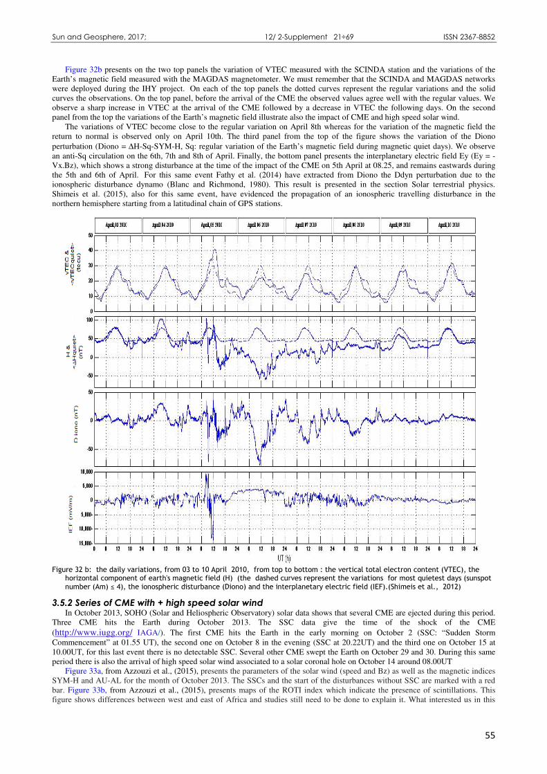
Sun and Geosphere, 2017; 12/ 2-Supplement 21÷69 ISSN 2367-8852
55
Figure 32b presents on the two top panels the variation of VTEC measured with the SCINDA station and the variations of the Earth’s magnetic field measured with the MAGDAS magnetometer. We must remember that the SCINDA and MAGDAS networks were deployed during the IHY project. On each of the top panels the dotted curves represent the regular variations and the solid curves the observations. On the top panel, before the arrival of the CME the observed values agree well with the regular values. We observe a sharp increase in VTEC at the arrival of the CME followed by a decrease in VTEC the following days. On the second panel from the top the variations of the Earth’s magnetic field illustrate also the impact of CME and high speed solar wind.
The variations of VTEC become close to the regular variation on April 8th whereas for the variation of the magnetic field the return to normal is observed only on April 10th. The third panel from the top of the figure shows the variation of the Diono
perturbation (Diono = ∆H-Sq-SYM-H, Sq: regular variation of the Earth’s magnetic field during magnetic quiet days). We observe an anti-Sq circulation on the 6th, 7th and 8th of April. Finally, the bottom panel presents the interplanetary electric field Ey (Ey = -Vx.Bz), which shows a strong disturbance at the time of the impact of the CME on 5th April at 08.25, and remains eastwards during the 5th and 6th of April. For this same event Fathy et al. (2014) have extracted from Diono the Ddyn perturbation due to the ionospheric disturbance dynamo (Blanc and Richmond, 1980). This result is presented in the section Solar terrestrial physics. Shimeis et al. (2015), also for this same event, have evidenced the propagation of an ionospheric travelling disturbance in the northern hemisphere starting from a latitudinal chain of GPS stations.
Figure 32 b: the daily variations, from 03 to 10 April 2010, from top to bottom : the vertical total electron content (VTEC), the
horizontal component of earth's magnetic field (H) (the dashed curves represent the variations for most quietest days (sunspot number (Am) ≤ 4), the ionospheric disturbance (Diono) and the interplanetary electric field (IEF).(Shimeis et al., 2012)
3.5.2 Series of CME with + high speed solar wind In October 2013, SOHO (Solar and Heliospheric Observatory) solar data shows that several CME are ejected during this period.
Three CME hits the Earth during October 2013. The SSC data give the time of the shock of the CME
(http://www.iugg.org/ IAGA/). The first CME hits the Earth in the early morning on October 2 (SSC: “Sudden Storm Commencement” at 01.55 UT), the second one on October 8 in the evening (SSC at 20.22UT) and the third one on October 15 at 10.00UT, for this last event there is no detectable SSC. Several other CME swept the Earth on October 29 and 30. During this same period there is also the arrival of high speed solar wind associated to a solar coronal hole on October 14 around 08.00UT
Figure 33a, from Azzouzi et al., (2015), presents the parameters of the solar wind (speed and Bz) as well as the magnetic indices SYM-H and AU-AL for the month of October 2013. The SSCs and the start of the disturbances without SSC are marked with a red bar. Figure 33b, from Azzouzi et al., (2015), presents maps of the ROTI index which indicate the presence of scintillations. This figure shows differences between west and east of Africa and studies still need to be done to explain it. What interested us in this

Amory-Mazaudier C. et.al. Recent Advances in Atmospheric, Solar-… PART B : Results and Capacity Building
56
figure is the absence of variations of the ROTI on 14th October over all Africa. Observing the Ascension ionosonde data we found that on the 14th October the layer F does not rise up after sunset as usual. We have explained this observation by the existence of a westward electric field inhibiting the normal Eastward electric field. It is this eastward electric field which lifts up the layer and allows the development of the instability of Rayleigh Taylor at the origin of scintillations in GPS signal. By using magnetic data, it was shown that this westward electric field opposite to the normal electric field was created by the ionospheric disturbance dynamo, DDEF, related to the high speed solar wind arriving at the Earth on 14th October 2013. This result is in agreement with the prediction of the model of Fejer et al., (2008) concerning the effect of the ionospheric disturbance dynamo.
These two examples clearly show the importance of studying long periods to truly understand the impacts of solar events on the ionosphere and develop Space Weather.
Figure 33 a: The solar wind parameters and geomagnetic indices for October 2013: (1) Vp the speed of the solar wind in km/s, (2)
the Bz component of the interplanetary magnetic field, (3) the Hsym index and (4) the AU and AL indices (Azzouzi et al., 2015)
A similar event was studied by Azzouzi et al., (2016) and Migoya-Orue et al., (2016). They showed that the impact of a high solar wind could be regional and in their case this high speed solar wind affected Africa and East America. More recently Rodriguez-Zugala et al., (2016) compared the different impact of a CME and a high speed solar wind on the Northern crest of the Equatorial Anomaly. They found that the response of the low-latitude ionosphere to solar phenomena is largely determined through the oscillation frequency of the IMF Bz by affecting the generation of the two mechanism of coupling between high and low latitudes PPEF and DDEF differently. This is seen as an effect of how the energy from the solar wind is transferred into the magnetosphere-ionosphere system.
3.6 GIC: Induced effects of the solar flare of 04 April, 1993 The induced effects of space weather related geomagnetic disturbances in the EEJ influence area are examined through the geo-
electric field variations in West Africa by Doumbia et al., (2017) [238] . In that purpose, variations of the North-South ( #) and East-West ( $) components of telluric electric field were analyzed, along with that of the three components (, & and ') of geomagnetic field during the geomagnetic storm of 17 February, 1993) and the solar flare observed on 04 April 1993 (See Doumbia et al., 2017 and references therein).
The geo-electric field responses to the ( that occurred around 14:30 LT on 4 April, 1993 are clearly observed at different stations (Figure 34). At LAM the crest to crest amplitude of the geo-electric field components associated with the ( are # =550/ and $ = 340/. Note that the ( impact on the geo-electric field variations decreases with the increasing distance of the stations from the sub-solar point, which is located at about 5.13°N on 4 April. This trend does not reflect the ( increasing amplitude near the dip-equator due the high Cowling conductivity in the EEJ belt.

Sun and Geosphere, 2017; 12/ 2-Supplement 21÷69 ISSN 2367-8852
57
Figure 33a: Maps of Tracks of GNSS satellites, around the observing stations for the events of October 2013. Pseudorandom noise
(PRN) codes of the satellites and scintillation timing of the corresponding L1 band scintillation are provided for each track (read color) (Azzouzi et al., 2015)

Amory-Mazaudier C. et.al. Recent Advances in Atmospheric, Solar-… PART B : Results and Capacity Building
58
These observations demonstrate that intense space weather events are potential sources of electric inductions within the Earth at low latitudes. The effectiveness of the induction effects of these geomagnetic field variations at low latitude is clearly shown through the geo-electric field observations. According to the observations shown is this work, the most important induction effects during the geomagnetic storm of 17 February 1993 and the solar flare of 04 April 1993 are associated with storm sudden commencement (*) and solar flare effect (() which are intense and rapid geomagnetic field variations.
Figure 34: Geo-electric field variations due to the solar flare on 04 April, 1993. The first line panels show variations of (left) and &
(right) and the second line panels show the time derivatives of (left) and & (right) at KOU. The other panels show variations of the $ (left colomn) and # (right colomn) at LAM, KOR, MOP and TOM (Doumbia et al., 2017)

Sun and Geosphere, 2017; 12/ 2-Supplement 21÷69 ISSN 2367-8852
59
3.7 Spread F/HF and Scintillations /GNSS
3.7.1 The Spread-F observed at Phu Thuy, Vietnam Using the vertical ionospheric sounding data observed at Phu Thuy observatory (21.029oN, 105.958oE), Vietnam in local night-
time from 1800LT to 0645LT for the 1962-1979 period, the occurrence characteristics of Spread-F was studied by Tran Thi Lan and Dao The Cuong (2013). During this period, the 15 minute film ionograms are obtained by the IRX (Hungarian) and AIC (Rusian) vertical ionospheric sounding systems. The statistic observations show that the most common types of spread-F observed at Phu Thuy are the range spread type (Fs_Q) and the frequency one (Fs_F). This result is different with the one of Hoang Thai Lan and Nguyen Thu Trang (2009) using the ionosonde data from Ho Chi Minh city observatory, South Vietnam, where the spurs spread F type (Fs_P) is observed more frequently. The spread-F occurrence frequency is calculated by the formula:
where T1 is the ionogram number with spread-F, T2 is ionograms lost by technical errors, T is total ionograms during night-time for the studied period(Figure SW6).
The statistical result shows that the maximum spread-F occurrence frequency of both types (Fs-Q and Fs-F) occurs after midnight at about 01 LT. In 1962-1979 period, the solar activity is devided into three levels: maximum (1969, 1970 and 1979 years), moderate (1962, 1963, 1966, 1971-1974) and minimum (1964, 1965, 1975-1977). The seasonal variation of Fs occurrence showed peaks at equinox months during the maximum solar phase, but in summer during the moderate and minimum solar activity (Figure 35). This result is similar to the one of Rastogi and Kulkarni (1969) using the data from Ahmedabad observatory in India and of Hoang Thai Lan and Nguyen Thu Trang (2009) for Ho Chi Minh city observatory in South Vietnam. The range spread-F occurs mainly before midnight on the equinox months and on the maximum solar phase. Meanwhite the frequency spread-F occurs mainly after midnight on summer and on the moderate and minimum solar activity.
Figure 35: Monthly occurrence frequency of spread-F at Phu Thuy for different solar phases, a) maximum, b) moderate and c)
minimum. (Tran Thi and Dao The, 2013)
100*(%)2
1
TT
Tf
−= (10)

Amory-Mazaudier C. et.al. Recent Advances in Atmospheric, Solar-… PART B : Results and Capacity Building
60
3.7.2 Scintillations observed at Kinshasa In the framework of the IHY project, 2 GPS stations of the SCINDA network have been installed in the DRC, one of them in
Kinshasa. Figure 36 (Kahindo et al., 2017) shows the S4 index (see sections 3.1) measured in 2012. The development of high amplitude scintillations (S4 > 1.0) is observed after 18UT (19.00 LT) just after the Pre Reversal Enhancement of the Electric Field (se tutorial section 1.8) and a maximum effect is observed during the equinoxes but the scintillation does not disappear during solstices. The interest of these observations is that they are obtained towards the southern ridge of the equatorial anomaly in a region where there are very few measurements. Satellite observations show ionospheric irregularities in the West African continent is more prolific event and occurs more frequently in Africa compared to other longitudinal sectors (Yigenzaw et al., 2014). It is important to develop networks of GNSS measurements in Africa
Figure 36: Scintillations observed at Kinshasa with the SCINDA GPS system (Kahindo et al., 2017)
Concluding remarks The effects of Space Weather are global so for GIRGEA as a community dealing with geophysics, it is a must to devote efforts to
improve the knowledge of the interactions between The Sun and The Earth., to deepen the subject please consult Knipp (2011) and Lilensten and Blelly (1999).
In this section, we have presented and commented on GNSS results obtained near the northern crest of the Equatorial Anomaly in the eastern and northern Africa (Shimeis et al., 2012 ; Azzouzi et al., 2015, Azzouzi et al., 2016), in Asia (Tran Thi Lan and Dao The Cuong, 2013) in America (Rodríguez-Zuluaga,2016), and also near the southern crest of the equatorial anomaly in Africa (Kahindo et al., 2017). All the studies related to Africa were possible thanks to the IHY and ISWI projects which enabled the deployment of GPS network in Africa.
In this section, we have shown the impact of coronal mass ejections or fast winds on the total electron content (TEC), the Earth’s magnetic field and the existence of scintillations. It is therefore essential to understand the Space Weather to develop systemic studies of the Sun-Earth system. It is also very important to have continuous measurements, ie observatories in order to realize the day-to-day effects.
4. Capacity building and societal development
Introduction All the results obtained and presented in sections 1, 2 and 3 were mainly obtained by PhD or post-doc students. In the majority of
cases new studies were introduced in the countries of the students, and students obtained positions at universities of their countries. In this section we will first present the international framework, then we will describe the curriculum established during these different projects and we will finish by the development and societal interests (SBAS).
4.1 Training and international projects The United Nations Basic Space Science Initiative (UNBSSI) was a long-term effort for the development of astronomy and space
science through regional and international cooperation. It covered an active transfer of technology and knowledge, and the role of education on a worldwide basis. To address the status of astronomy, a series of workshops on basic space science was held from 1994 to 2004. In line with one of the major recommendations emanating from these workshops, the establishment of astronomical

Sun and Geosphere, 2017; 12/ 2-Supplement 21÷69 ISSN 2367-8852
61
facilities in developing nations for research and education programmes at the university level was initiated. From 2004, the initiative continued through a series of annual workshops dedicated to to the International Heliophysical Year of 2007 (IHY). IHY’s legacy is the operation of 16 worldwide instrument arrays with more than 1000 instruments recording data on solar-terrestrial interaction from coronal mass ejections to variations of the total electron content in the ionosphere. The International Space Weather Initiative (ISWI) is a follow-up activity to IHY, focusing exclusively on space weather.
The International Committee on Global Navigation Satellite Systems (ICG), established in 2005, promotes cooperation on matters related to civil satellite-based positioning, navigation, timing, and value-added services. The ICG works to enhance coordination among providers of global navigation satellite systems (GNSS), regional systems, and augmentations in order to ensure greater compatibility, interoperability, and transparency, and to promote the introduction and utilization of these services and their future enhancements with the integration into their infrastructures. Within the framework of the ICG workplan, GNSS applications in low-cost worldwide ground-based instrument arrays for exploring atmospheric phenomena related to space weather have been considered in the ICG working group information dissemination and capacity-building. As the body leading the working group, the United Nations Office for Outer Space Affairs, through its programme on GNSS applications, each year co-organizes and co-sponsors a wide range of seminars, training courses and workshops. Those activities usually bring together a large number of experts, including specialists from developing countries, to discuss the GNSS applications in various fields of the world economy.
Additionally, a series of activities are undertaken at the regional centres for space science and technology education, affiliated to the United Nations, also acting as the ICG information centres. These activities emphasize the development and enhancement of the knowledge and skills of university educators and research and application scientists in both the physical and natural sciences as well as in analytical disciplines.
4.2 Cursus In the course of the IHY project, the necessity to approach the Sun Earth system in an integrated way appeared essential to
progress in the knowledge. The ISWI project on Space Weather with the deployment of GNSS and magnetometer stations led to the development of training on the processing and analysis of GNSS and magnetic data.
4.2.1 Training on the Solar terrestrial physics in an integrated framework This course was taught at a school with professors from all disciplines and with teachings on the Sun, magnetosphere, ionosphere,
atmosphere and terrestrial magnetic field. SCOSTEP (http://www.yorku.ca/scostep/, the regional Center of United Nations, CRASTE-LF (http://www.crastelf.org.ma/)
and our network organized many schools reported on different websites : http://ihy2007.org , http://www.iswi-secretariat.org,
http://wwwoosa.unvienna.org.
4.2.2 Analysis and processing of GNSS data for the different disciplines This training was developed by ICTP (https://www.ictp.it), Boston University (http://www.bu.edu/)
and the National French school of Telecommunications of Brest (Amory-Mazaudier and Fleury, 2012). In the GIRGEA network the training on GNSS was mainly assumed by the National French school of Telecommunications. The course of Rolland Fleury is on
the website http://wwwoosa.unvienna.org, (Amory-Mazaudier et al., 2017a, 2017b).
Analysis and interpretation of magnetic data for the different disciplines The training was developed by the Kyushu University https://www.kyushu-u.ac.jp/en/ in charge of the network of magnetometer
MAGDAS. In our network we developed a training on magnetic data based on the dynamos and their associated electric currents system in the Sun-Earth system (Amory-Mazaudier, 2009).
Finally, all the schools now include courses on the Solar Terrestrial physics with a training on the different data available on the web. In the framework of the French Egyptian year, we teached on the Sun Earth system and GNSS applied to all the disciplines: geodesy, atmospheric physics and ionospheric physics (Dame et al., 2010).
4.3 GNSS development in DRC There are many GNSS stations in Africa, developed as part of several projects. Some have been set up for tectonics (mainly
along the East African rift (EAR), from Djibouti and Ethiopia to Malawi), others for meteorological studies, others for the study of the ionosphere. These GNSS stations have been used to define the large-scale tectonics of the area, and specially the movements of the plates Nubia (west of the EAR) and Somalia (east of the EAR) (Stamps et al. (2008), Deprez et al.(2013), Saria et al. (2014). These networks have heterogeneous coverage, which leaves the Democratic Republic of Congo (DRC) relatively poorly covered. That's why we decided to set up new stations in the DRC (Figure 37). These stations have 3 scientific objectives. 1- Improve the overall coverage of the Nubia plate (Africa West of the East African rift) and the calculation of the pole of rotation of this plate. 2- Improve the kinematics at a regional scale between the DRC and Tanzania for a better understanding of the function of the rift at this place. 3- Characterize the deformations of the Congo basin, which are certainly weak but perhaps not zero.
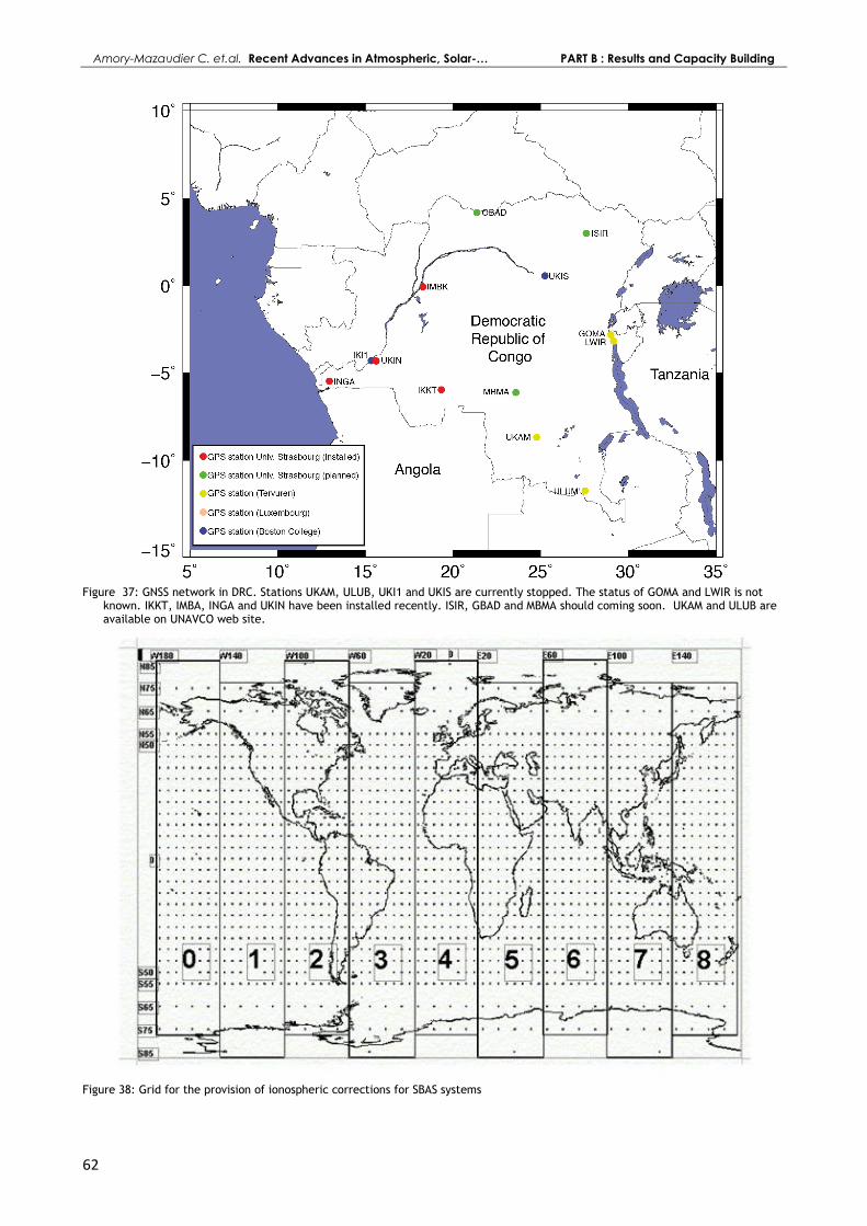
Amory-Mazaudier C. et.al. Recent Advances in Atmospheric, Solar-… PART B : Results and Capacity Building
62
Figure 37: GNSS network in DRC. Stations UKAM, ULUB, UKI1 and UKIS are currently stopped. The status of GOMA and LWIR is not
known. IKKT, IMBA, INGA and UKIN have been installed recently. ISIR, GBAD and MBMA should coming soon. UKAM and ULUB are available on UNAVCO web site.
Figure 38: Grid for the provision of ionospheric corrections for SBAS systems

Sun and Geosphere, 2017; 12/ 2-Supplement 21÷69 ISSN 2367-8852
63
4.4 Satellite-Based Augmentation System (SBAS) Satellite-Based Augmentation System (SBAS) refers to a system offering corrections to improve the accuracy of positioning on a
regional coverage. It covers WAAS (USA + Canada), EGNOS (Europe), MSAS (Japan), GAGAN (India). Like the GPS system, it is composed of 3 segments:
Land component:
• a network of reference stations operating in real time, equipped with very precise clocks and which records the raw measurements (pseudo-distances and phases)
• a treatment center (s), which makes the corrections
• navigation ground stations (NLES) which transmit to the corrections to the space component Spatial component includes geostationary satellites re-transmitting corrections on the GNSS L1 (free public service)
frequency and on the L5 frequency (aviation-specific) to the user component User component consisting of specific receivers that pick up GPS signals and, in addition, the geostationary signal and which
contain specific software to make corrections on their specific position Errors are identified according to their origin and therefore individualized in specific messages
• - The ionospheric error restored on a fixed geometric grid (see figure 38)
• - drift of GPS clocks
• - Corrections to improve the orbit of GPS satellites. + The integrity of the system. Objectives:
• - 3-4 m error for 95% of the time for public access
• - Less than 1 m for civil aviation. EGNOS is operational and covers Europe to the Mediterranean coast in Africa. The challenge for the coming years is to extend it
more towards the equator. The network of ground stations already includes Agadir (Morocco), the Canary Islands, Nouakchott (Mauritania), Djerba (Tunisia), Alexandria (Egypt) and Tamanrasset (Algeria) and Abu Simbel (Egypt) to come up).
However, regarding the ionosphere, they are aware of the specific problem of low latitudes: The strong gradients of TEC lower than their mesh of the grid, presented in figure 58, and thus not detected by their network
of reference stations. In our opinion, their grid is not thin enough for the lower latitudes, it was made by an administrative and not by a physicist.
Scintillation which distorts the phase measurements and therefore degrades the positioning, - EPBs, which are associated with local gradients and scintillation,
Conclusion: there are works on TEC and scintillations for African scientists, they have to look for extreme scenarios
and better control the climatology of these phenomena.
Concluding remarks In the GIRGEA network, the collective work in the framework of international cooperation has produced many results; During
the last decade [ 2006-May 2017], 29 PhD were defended in the following countries: Algeria, DRC, Egypt, Burkina Faso, Côte d'Ivoire, Morocco, Senegal, Vietnam, and all the students obtained positions in their countries.
We have been able to develop new courses which are now part of university curricula in countries. With the deployement of GNSS receivers all over the world, GNSS has become one of the most powerful tools to develop
Ionosphere studies with a very large number of instruments, which, however, remains very inadequate in Africa. It is therefore necessary to develop the GNSS network in Africa because GNSS allows scientific studies in many disciplines (atmosphere, ionosphere, geodesy, etc.) and many applications (agriculture, navigation, etc...).
Space weather is essential for understanding the impacts of solar events on new technologies and in particular on GNSS.
General Conclusion The works presented in this article is only part of the results obtained during the last decade in the framework of the IHY and
ISWI projects, those of our GIRGEA network. It is difficult to re-read all the results which are generally given in concluding remarks at the end of each part. Most importantly, during the last ten years, the scientific studies in Africa, Asia and in the countries of the South, in the fields presented have increased sharply, and this thanks to scientific associations and the United Nations. An important transfer of knowledge and working methods has made it possible to have teams with whom we can fully continue cooperation on an equal footing.
Acknowledgement Our appreciation is for Art Richmond, now retired, who has participated in numerous training schools in Africa and has
supervised students from Cote d'Ivoire, Burkina Faso, Spain and Vietnam. We thank all observers who collect the magnetic observations in the different networks of magnetometers and particularly the INTERMAGNET and MAGDAS networks. We thank all the providers of GNSS data and particularly the IGS, UNAVCO and SCINDA networks. We thank all scientists from the ISWI network and all those who have organized schools or courses in the schools of the IHY, ISWI and SCOSTEP projects. We thank all universities and international organizations that have contributed to this work and especially: UPMC, The French National school of telecom/Brest, Kyushu University, Boston College, UNOOSA , ICTP, ICG.
The continuous GPS network in Vietnam has been installed in frame of the cooperation between the Institute of Geophysics, Vietnam Academy of Science and Technology and the Rennes 1 University (French), the Mines-Telecom Bretagne (French), the National Taiwan University, the National Institute of Information and Communication Technology (Japan). Pham Thi Thu H. is supported by the research project of Vietnam Foundation for Technology Development (NAFOSTED) under grant 105.05-2014.30.

Amory-Mazaudier C. et.al. Recent Advances in Atmospheric, Solar-… PART B : Results and Capacity Building
64
References
B. O. Adebesin, A.B. Rabiu J.O. Adeniyi, C. Amory-Mazaudier, Nighttime morphology of vertical plasma drifts at Ouagadougou during different seasons and phases of sunspot cycles 20–22, J. Geophys. Res. Space Physics 120 (2015) pp. 4223-4229. doi:10.1002/2015JA021737.
J-P. Adohi, P. Vila, C. Amory-Mazaudier, M. Petitdidier, Equinox transition at the magnetic equator in Africa: Analysis of ESF ionograms,Ann. Geophys. 26, 7 (2008) pp 1777-1792.
S.J. Allen, R.A. Vincent, Gravity wave activity in the lower atmosphere: seasonal and latitudinal variations, J. Geophys. Res. 100 (1995) pp 1327-1350.
R.I. Albrecht, S.J. Goodman, D.E. Buechler, R.J. Blakeslee, H.J. Christian, Where are the lightning hotspots on Earth?, Bull. Am. Meteorol. Soc. 97, 2 (2016) pp. 2,051- 2,068. doi:10.1175/bams-d-1400193.1.
P. Alken, S. Maus, Spatio-temporal characterization of the equatorial electrojet from Champ, Orsted and SAC-C satellite magnetic measurements, J. Geophys. Res. – Space Phys. 112, (2007) pp. 1978-2012. doi:10.1029/2007/JA012524.
C. Amory-Mazaudier, Electric Current Systems in the Earth’s Environment, Nigerian J. Space Res. 8 (2010) pp. 178-255 . ISSN 0794-4489.
C. Amory-Mazaudier, R. Fleury, Space Research in Africa, some achievements from 2007 to 2012, Sun and Geosphere 8, 2, (2013) pp. 65-70. ISSN 1919-0839.
C. Amory-Mazaudier, R. Fleury, S. Gadimova, A. Touzani, Touzani , Space Weather, from the Sun to Earth, the key role of Global Navigation Satellite Systems, Part I : From the Sun to the Earth, Space Weather and its effects, Coordinates February (2017a)
pp. 6-14. http://www.mycoordinates.org C. Amory-Mazaudier, R. Fleury, S. Gadimova, A. Touzani, , Space Weather from the sun to the Earth, the key role of Global
Navigation Satellite Systems- Part II: Training on daily global positioning system GPS data , Coordinates March (2017b) pp 31-35. http://www.mycoordinates.org
F. Anad, C. Amory-Mazaudier, M. Hamoudi, S. Bourouis, A. Abtout, E. Yizengaw, Sq solar variation at Médéa Observatory (Algeria), from 2008 to 2011, Adv. Space Res. 58, 9, (2016) pp 1682. doi10.1026/j.asr. 2016.06029
T.T. Ayorinde, B. Rabiu, C. Amory-Mazaudier, Inter-hourly Variability of Total Electron Content during the quiet condition over Nigeria, within the Equatorial Ionization Anomaly region, J. Atmos. Sol. Terr. Phys. 145 (2016 ) pp. 21-33.
I. Azzouzi, Y. Migoya-Orué, C. Amory Mazaudier, R. Fleury, S. M. Radicella, A. Touzani, Signatures of solar event at middle and low latitudes in the Europe-African sector, during geomagnetic storms, October 2013, Adv. Space Res. 56, 9, (2015) pp 2040. doi:
10.1016/j.asr.2015.06.010. I. Azzouzi, Y. Migoya-Orué, P. Coïsson, C. Amory Mazaudier, R. Fleury, S.M. Radicella Day-to day variability of VTEC and ROTI in
October 2012 with impact of high-speed solar wind stream on 13 October 2012, Sun and Geosphere 11, 1 (2016) pp. 7-22. ISSN 2367 8852.
I. Azzouzi, Impact des évènements solaires sur l’ionisation de l’ionosphère des moyennes et basses latitudes dans le secteur Europe-Afrique, 238p, Thèse Université P. et M. Curie, France & Université Mohammed V de Rabat, Maroc (2016) available in the data base La Hal.
G. Balasis, I.A. Daglis, P. Kapiris, M. Mandea, D. Vassiliadis, K. Eftaxias, , From pre-storm to magnetic storms: a transition described in terms of fractal dynamics, Ann. Geophys. 24 (2006) pp. 3557-3567.
L. Benkevitch, W. Lyatsky, L.L. Cogger, Field aligned currents between Conjugate hemispheres, J. Geophys. Res. 105, A12 (2000) pp 27727-22737. doi:10.1029/2000JA900095
D. Bilitza, D. Altadill, Y. Zhang, C. Mertens, C. Truhlik, P. Richards, L-A McKinnell, B. Reinisch, The International Reference Ionosphere 2012 –a model of international collaboration, Journal of Space Weather and Space Climate., Journal Space Weather and Space Climate 4, A07 (2014). doi:10.1051/swsc/2014004.
M. Blanc, A.D. Richmond, The ionospheric disturbance dynamo, J. Geophys. Res., 85, A4 (1980), pp. 1669-1686, doi: 10.1029/JA085iA04p01669
E. Blanch, S. Marsal, A. Segarra, J.M. Torta, D. Altadill, J-J. Curto, Space Weather effects on Earth’s environment associated to the 24-25 October 2011 geomagnetic storm, Space Weather 11, (2013) pp. 153-168. doi:10.1002/swe.20035.
O.S. Bolaji, E.O. Oyeyemi, O. Owolabi, Y. Yamazaki, A. B. Rabiu, D. Okoh, D., A. Fujimoto, C. Amory Mazaudier, A. Yoshikawa, Solar quiet current
response in the African sector due to a 2009 sudden stratospheric warming event" , J. Geophys. Res., Space Physics, 121 (2016) pp. 8055-
8065. doi:10.1002/2016JA022857.
C. G. M. Brum, C. A. Tepley, J.T. Fentzke, E. Robles, P. T. dos Santos, S.A. and Gonzalez, Long-term changes in the thermospheric neutral winds over Arecibo: Climatology based on over three decades of Fabry-Perot observations, J. Geophys. Res., Space, 117, A00H14 (2012). doi:10.1029/2011JA016458.
R. E. Burgesser, M. G. Nicora, E.E. Avila, Characterization of the lightning activity of ‘’Relampago del Catatumbo’ J. Atmos. Sol. Terr. Phys. (2012). doi :10.1016j.jastp.2012.01.013.
T. Chang, Self-organized criticality, multi-fractal spectra, sporadic localized reconnections and intermittent turbulence in magnetotail, Phys. Plasmas 6 (1999) pp. 4137-4145.
H. J. Christian, R. J. Blakeslee, D. J. Boccippio, W. L. Boeck, D. E. Buechler, K. T. Driscoll, S.J. Goodman, J. M. Hall, X.J. Koshak, D. M. Mach, M. F. Stewart, M. F., Global frequency and distribution of lightning as observed from space by the Optical Transient Detector, J. Geophys. Res. 108, D1, (2003) pp. 4005, doi:10.1029/2002JD002347.
I. Cnossen, A.D. Richmond, , Modelling the effects of changes in the Earth's magnetic field from 1957 to 1997 on the ionospheric hmF2 and foF2 parameters, J. Atmos. Sol. Terr. Phys. 70 (2008), pp 1512-1524. doi:10.1016/j.jastp.2008.05.003.
I. Cnossen, A. D. Richmond, M. Wiltberger, The dependence of the coupled magnetosphere-ionosphere thermosphere system on the Earth’s magnetic dipole moment, J. Geophys. Res. 117, A05302 (2012). doi:10.1029/2012JA017555.
I.Cnossen, A. D. Richmond, How changes in the tilt angle of the geomagnetic dipole affect the coupled magnetosphere- ionosphere-thermosphere system, J. Geophys. Res. 117, A10317 (2012). doi: 10.1029/2012JAA0118056.
K. D. Cole, Magnetic storms and associated phenomena, Space Sci. Rev. 5 (1966) pp 699-770. D. Reidel Publishing Company, Dordrecht, Holland.
A.B. Collier, A. R. W. Hughes, Lightning and the African ITCZ J. Atmos. Sol.-Terr. Phys. 73 (2011) pp. 2392-2398. doi:10.1016/j.jastp.2011.08.010.
A. J. Coster, M. Colerici, J. Foster, B. Rideout, F. Rich, F., B. Taylor, Magnetic conjugacy of storm enhanced density, Abstract 31370, National Radio Science Meeting, 4-7, University of Colorado, Boulder (2006).
J-J. Curto, T. Araki, L. F. Alberca, Evolution of the concept of Sudden Storm Commencements and its operative identification, Earth Planets and Space 59,11 (2007) pp 1.

Sun and Geosphere, 2017; 12/ 2-Supplement 21÷69 ISSN 2367-8852
65
J-J. Curto, M. Blanca, E. Martínez, ., Automatic Sunspots detection on Full-disk Solar images using mathematical morphology, Solar Phys. (2008). doi: 10.1007/s11207-008-9224-6.
J-J. Curto, L.R. Gaya-Piqué, Geoeffectiveness of Solar Flares in magnetic crochet (sfe) Production: I - Dependence on their spectral nature and position on the solar disk, J. Atmos. Sol. Terr. Phys. 71 (2009a) pp 1695-1704. doi. 10.1016/j.jastp.2008.06.018.
J-J. Curto, L. R. Gaya-Piqué, Geoeffectiveness of Solar Flares in magnetic crochet (sfe) Production: II - Dependence on the detection method, J. Atmos. Sol. Terr. Phys. 71 (2009b) pp 1705-1710. doi: 10.1016/j.jastp.2007.12.003.
J-J. Curto, E. Also, E. Pallé, J. G. Solé, Sunshine and synoptic cloud observations at Ebro Observatory, International J. Climatology 29 (2009c) pp. 2183-2190. doi: 10.1002/joc.1841.
J-J. Curto, J. Castell, F. Del Moral, F., Sfe: waiting for the big one, J. Space Weather and Space Climate (2016). doi: 10.1051/swsc/2016018.
L. Damé, A. Mahrous, C. Amory-Mazaudier, M. Petitdidier, A. Hady, , Météorologie de l’Espace en Afrique (1) Année Franco-Egyptienne de la Science et de la Technologie 2010, REE 6/7 (2010) pp. 114-120.
A. Déprez, C. Doubre, F. Masson, P. Ulrich P., Seismic and aseismic deformation along the East African Rift System from a reanalysis of the GPS velocity field of Africa, Geophys. J. Int., 193 (2013) pp. 1353-1369. doi:10.1093/gji/ggt085
E. R. De Paula, F. S. Rodrigues, K. N. Iyer, I. J. Kantor, M. A. Abdu, P. M. Kintner, B. M. Ledvina, H. Kintner, Equatorial anomaly effects on GPS scintillations in Brazil, Adv. Space Res. 31 (2003) pp. 749-754. doi:10.1016/S02731177(03)00048-6.
D. T. De Wit, I. Ermolli, M. Haberreiter, H. Kambezidis, M. M. Lam, J. Lilensten, K. Matthes, I. Mironova, H. Schmidt, A. Seppala, E. Tanskanen, K. Tourpali, Y. and Yair, , Earth’s climate response to a changing Sun, EDP Sciences (2015). ISBN: 978-2-7598-1733-7.
Y. Ding, L. Yanju, Onset and the evolution of the Summer Monsoon over the South China Sea during SCSMEX Field Experiment in 1998, J. Meteor.
Soc. Japan 79 (2001) pp. 255-276.
V. Doumbia, A. Maute, A. D. Richmond, Simulation of equatorial electrojet magnetic effects with the thermosphere-ionosphere-electrodynamics general circulation model, J. Geophys. Res. 112, A09309 (2007). doi:10.1029/2007JA012308.
V. Doumbia, K. Boka, N. Kouassi, O. D. F. Grodji, C. Amory-Mazaudier, M. Menvielle, Induction effects of geomagnetic disturbances in the geo-electric field variations at low latitudes, Ann. Geophys. 35 (2017) pp. 39-51. doi:10.5194/angeo-35-39-2017.
V. Doumbia, F. Grodgi, On the Longitudinal Dependence of the Equatorial Electrojet, Monograph 220, First Edition. (2017).Fuller-Rowell, T., Yizengaw, E., Doherty, P.H., and Basu, S. (Eds). American Geophysical Union, John Wiley & Sons, Inc. pub.
V. Doumouya, Y. Cohen, Y., Local time and longitude dependence of the equatorial electrojet magnetic effects, J. Atmos. Sol. Terr. Phys. 65 (2003) pp. 1265-1282.
D. P. Drob, J. T. Emmert, J. W. Meriwether, J. J Makela, E. Doornbos, M. Conde, G. Hernandez, J. Noto, K. A. Zawdie, S. E. McDonald, J. D. Huba, J. H Klenzing, J. H., An update to the Horizontal Wind Model (HWM): The quiet time thermosphere, Earth Space Sci. 2 (2015) pp. 301-319, doi:10.1002/2014EA000089
A. G. Elias, N. Ortiz de Adler, Earth magnetic field and geomagnetic activity effects on long term trends in the F2 layer at mid-high latitudes, J. Atmos. Solar Terr. Phys. 68 (2006) pp. 1871-1878 , doi:10.1016/j.jastp.2006.02.008.
A. G. Elias, Trends in the F2 ionospheric layer due to long-term variations in the Earth's magnetic field, . Atmos. Solar Terr. Phys. 71 (2009) pp. 1602-1609. doi:10.1016/j.jastp.2009.05.014.
I. Fathy, C. Amory-Mazaudier, A. Fathy, A. M. Mahrous, K. Yumoto, K., E. Ghamry, Ionospheric disturbance dynamo associated to a coronal hole:Case study 5-10 April 2010, J. Geophys. Res. (2014). doi10.1002/2013JAO19510
O. Fambitakoye, M. Menvielle, C. Mazaudier, Global disturbance of the transient magnetic field associated to thermospheric storm winds on 14arch 23, 1979, J. Geophys. Res. 95, A9 (1990) pp. 209-218.
B. G. Fejer, J. W. Jensen, S.-Y. Su, Seasonal and longitudinal dependence of equatorial disturbance vertical plasma drifts, Geophys. Res. Lett. 35, L20106 (2008). doi :10.1029 /2008GL035584
B. G. Fejer, E. R. Depaula, S. A. Gonzalez, R. F. Woodman, Average vertical and zonal F region plasma Drifts over Jicamarca, J. Geophys. Res. 96, A8 (1991) pp 13,901.
D. J. Fisher, J. Makela, J. W. Meriwether, R. A. Buriti, Z. Benkhaldoun, M. Kaab, A. Lagheryeb, Climatologies of nighttime thermospheric winds and temperatures from Fabry-Perot interferometer measurements: From solar minimum to solar maximum, J. Geophys. Res.- Space Physics, 120, 8 (2015) pp. 6679-6693. doi:10.1002/2015JA021170.
A.J. Foppiano, L. Cid, V. Jara , Ionospheric long-term trends for South American mid-latitudes,J. Atmos. Sol. Terr. Phys. 61 (1999) pp 717-723.
D. C. Fritts, M. J. Alexander, Gravity wave dynamics and effects in the middle atmosphere, Rev. Geophys. 41 (2003) pp. 1003. D. A. Gnabahou, F. Ouattara, Ionosphere variability from 1957 to 1981 at Djibouti station, European Journal of Scientific Research
73,3 (2013) pp 382. D. A. Gnabahou, A. G. Elias, F. Ouattara, F., Long-term trend of foF2 at a West African equatorial station linked to greenhouse gas
increase and dip equator secular displacement, J. Geophys. Res. 118 (: 2013) pp. 3909-3913. doi:10.1002/jgra.50381. A. Gómez, J. J. Curto, C. Gras, C., Evolution of sunspot’s characteristics in cycle 23, Solar Phys. 289 , 1 (2014) pp. 91- 106.
doi:10.1007/s11207-013-0323-7. F.O. Grodji, V. Doumbia, K. Boka, C. Amory-Mazaudier, Y. Cohen, R. Fleury, R., , Estimating some parameters of the equatorial
ionosphere electrodynamics from ionosonde data in West Africa, Adv. Space Res. 59 (2017) pp. 311-325. M.E. Hagan, J.M. Forbes, Migrating and nonmigrating diurnal tides in the middle and upper atmosphere excited by tropospheric
latent heat release, J. Geophys. Res., 107, D24 (2002) pp. 4754. doi:10.1029/ 2001JD001236. M.E. Hagan, J.M. Forbes, Migrating and nonmigrating semidiurnal tides in the upper atmosphere excited by tropospheric latent heat
release, J. Geophys. Res., 108, A2 (2003) pp 1062. doi:10.1029/2002JA009466. A. E. Hedin, Extension of the MSIS thermosphere model into the middle and lower atmosphere, J. Geophy. Res. 96 (1991) pp. 1159. G.J. Holland, Interannual Variability of the Australian Summer Monsoon at Darwin: 1952-82, Mon. Wea. Rev. 114 (1986) pp 594-604. S. B. Henderson, C. M. Swenson, A. B. Christensen, L. J. Paxton, Morphology of the equatorial anomaly and equatorial plasma
bubbles using subspace analysis of Global Ultraviolet Imager data, J. Geophys. Res. 110, A11306 (2005). doi:10.1029/2005JA011080.
L. Hoang Thai, T. T. Nguyen, Some characteristics of equatorial spread F observed in Vietnam, J. Earth Sci. 31, 4 (2009) pp. 368-373 (in Vietnamese, abstract in English).
A. T. Kobea, A. D. Richmond, B. A. Emery, C. Peymirat, H. Luhr, T. Moretto, M. Hairston,C. Amory-Mazaudier, Electrodynamic Coupling of High and Low Latitudes Observations on May 27,1993, J. Geophys. Res. 105, A10 (2000) pp. 22979-22989.
M. Kaab, Z. Benkhaldoun, D. J. Fisher, B. Harding, A. Bounhir, J. Makela, A. Laghriyeb, K. Malki, A. Daassou, M. Lazrek, Climatology of thermospheric neutral winds over Oukaïmeden Observatory in Morocco, Ann. Geophys. 35 (2017) pp. 161-170. doi:10.5194/angeo-35-161-2017.

Amory-Mazaudier C. et.al. Recent Advances in Atmospheric, Solar-… PART B : Results and Capacity Building
66
P. Kafando, F. Chane-Ming, M. Petitdidier, Climatology of gravity waves activity during the West African monsoon, Ann. Geophys. 26 , 12 (2008) pp. 4081-4089.
P. Kafando, F. Chane-Ming, M. Petitdidier, Stratospheric variability of wave activity and parameters in equatorial coastal and tropical sites during the West African monsoon J. Clim. Dyn. (2015). doi:10.1007/s00382-015-2764-1.
B. Kahindo, A. Kazadi, R. Fleury, F. Tondozi Keto, A. Zana Ndontoni, M. Kakule Kaniki, C. Amory-Mazaudier, K. Groves, Contribution à l’étude de la scintillation ionosphérique équatoriale sur la crête sud de l’Afrique submitted to Journal des sciences.
Y. Kamide, N. Fukushima , Positive geomagnetic bays in evening high latitudes and their possible connection with partial ring current,Rep. ionos. Space Res. Jap. 26 (1972) pp. 79-101.
H. Kim, X. Cai,C. R. Clauer, B. S. R. Kunduri, J. Matzka, C. Stolle, D. R. Weimer, Geomagnetic response to solar wind dynamic pressure impulse events at high latitude Conjugate points, J. Geophys. Res. 118, 10 (2013) pp. 6055-6071. doi:10.1002/jgra.50555.
D. J. Knipp, Understanding Space Weather and the Physics behind it. Publisher Mc Graw-Hill Education Europe, (2011). ISBN 10:0073408905.
P. Kovacs, V. Carbone, Z. Vörös, Z., Wavelet based filtering events from geomagnetic time-series, Planet. Space Sci. 49 (2001) pp. 1219-1231.
A. Laraque, J. P. Bricquet, A. Pandi, J. C. Olivry, A review of material transport by the Congo River and its tributaries, Hydrol. Process 23 (2009) pp. 3216-3224.
K. Laundal, M. N. Østgaard, K. Snekvik, H.U. Frey, H. U., Interhemispheric observations of emerging polar cap asymmetries, J. Geophys. Res. 115, A07230 (2010). doi: 10.29/2009JA015160.
L. Lastovicka, S.C. Solomon, L. Qian, Trends in the Neutral and Ionized Upper Atmosphere, Space Sci. Rev. 168 (2012) pp. 113-145. doi:10.1007/s11214-011-9799-3.
K.M. Lau, S. Yang, Climatology and Interannual Variability of the Southeast Asian Summer Monsoon, Adv. Atmos. Sci. 14 (1997) pp. 231-245.
J-P. Legrand, P. Simon, A review for geophysicists: Part I : The contribution to geomagnetic activitu of shock waves and of the solar wind, Ann. Geophys., 7, 6, (1989) pp 565-578.
M. Le Huy, C. Amory-Mazaudier, Magnetic signature of the ionospheric disturbance dynamo at equatorial latitudes: “Ddyn”, J. Geophys. Res., 110, A10301 (2005). doi:10.1029/2004JA010578.
M. Le Huy, C. Amory-Mazaudier, Planetary magnetic signature of the storm wind ionospheric disturbance dynamo currents: “Ddyn”, J. Geophys. Res. 113, A02312 (2008). doi:10.1029/2007JA012686.
M. Le Huy, C. Amory-Mazaudier, R. Fleury, A. Bourdillon, P. Lassudrie-Duchesne, L. Tran Thi, T. Nguyen Chien , T. Nguyen Ha, P. Vila, Time variations of the total electron content in the Southeast Asian equatorial ionization anomaly for the period 2006-2011, Adv. Space Res. 54 (2014) pp. 355-368.
M. Huy, L. Tran Thi, R. Fleury, C. Amory Mazaudier, T. Le Truong, T. Nguyen Chien, T. Nguyen Ha, TEC variations and ionospheric disturbances during the magnetic storm on March 2015 observed from continuous GPS data in the Southeast Asian region, Vietnam J. Earth Sci. 38, 3 (2016) pp. 287-305. doi:10.15625.0866-7187/38/3/8714, ISBN 0866-7187.
T. Le Truong, V. Doumouya, M. Le Huy, C. Ha Duyen, The equatorial electrojet model with Champ data, Vietnam J. Earth Sciences 32, 1, (2010) pp. 48-57 (in Vietnamese, abstract in English).
T. Le Truong, M. Le Huy, C. Ha Duyen, V. Doumouya, Y. Cohen, Anomaly of equatorial electrojet (EEJ) and its seasonal variation, Vietnam J. Earth Sciences 33, 1 (2011) pp 29-36 (in Vietnamese, abstract in English).
C. Li, M. Yanai, he Onset and Interannual Variability of the Asian Summer Monsoon in Relation to Land-Sea Thermal Contrast, J. Climate 9 (1996) pp. 358-375.
J. Lilensten, P.-L. Blelly, Du Soleil à la Terre, Aéronomie et météorologie de l'espace. Presses Universitaires, Collection Grenoble Sciences, Université Joseph Fourier Grenoble I (1999). ISBN 9782868834676.
A.T.Y. Lui, Multiscale phenomena in the near-Earth magnetosphere, Atmos. Sol.-Terr. Phys. 64 (2002) pp. 125-143. H. Luu Viet, Etude du champ électromagnétique et interprétation des données magnétotelluriques au Vietnam, Thèse soutenue le
21 décembre Université Paris Sud 11, France (2011). H. Luu Viet, M. Menvielle, M. Le Huy, Study of the effect of the equatorial electrojet on magneto-telluric soundings in Southern
Vietnam, Proceedings of the 2nd International Conference on Green Technology and Sustainable Development, Ho Chi Minh Ville /Bamgladesh, 5-6 September (2014a) pp 26 – 34.
H. Luu Viet, M. Menvielle, M. Le Huy, S. Vo Thanh, T. Nguyen Chien, G. Marquis, T. Cao Dinh, Studying the deep structure in the Sai Gon River fault area by the magnetotelluric method, Vietnam J. Earth Sciences 36, 3 (2014b) pp. 233-240. ISBN 0866-7187.
D. R. MacGorman, W.D. Rust,The electrical nature of storms (1998). Oxford University Press, New York,USA. A.M. Mahrous, O. A. AbuElezz, A. M. Abdallah, R.Fleury, Comparison between the NeQuick model and VTEC estimation by GPS
measurements over Egypt, Intech, chapter 14 (2014). doi:10.5772/58773. P. J. Mann, R. G.M. Spencer, J. B. Dinga, J. R. Poulsen, P.J. Hernes, G. Fiske, M. E. Salter, Z. A. Wang, K. A. Hoering, J. Six, R. M.
Holmes, The biogeochemistry of carbon across a gradient of streams and rivers within the Congo Basin, J. Geophys. Res. (2014). doi: 10.1002/2013JG002442 .
J. Mao, J. C. L. Chan, G. Wu, G., Relationship between the Onset of the South China Sea Summer Monsoon and Structure of the Asian Subtropical Anticyclone, J. Meteor. Soc. Japan 82 (2004) pp. 845-859.
J. Matsumoto, Seasonal Transition of Summer Rainy Season over Indochina and Adjacent Monsoon Region, Adv. Atmos. Sci. 14 (1997) pp. 231-245.
P. N. Mayaud, Analyse morphologique de la variabilité jour-à-jour de la variation journalière régulière SR du champ magnétique terrestre, I- le système de courants Cp (régions polaires et subpolaires), Ann. Géophys. 21 (1965) pp. 369-401.
P. N. Mayaud, Sur quelques propriétés de l’activité magnétique déduites de l’analyse d’une série de neuf années des indices Kn, Ks et Km ; I- Comparaison des niveaux d’activité dans chaque hémisphère, Ann. Géophys. 26 (1970) pp. 109-126.
C. Mazaudier, Electric currents above Saint-Santin: 1. Data, J. Geophys. Res. 87 (1982) pp. 2459-2464. M. N . Mene, A.T. Kobéa, O. Obrou, K. Z. Zaka, K. Boka, C. Amory- Mazaudier, P. Assamoi, Statistical study of the DP2 enhancement
at the dayside dip-equator compared to low latitudes, Ann. Geophys. (2011) pp. 2225-2233. M. N. Mene, Etude Statistique du phénomène de pénétration du champ électrique de convection magnétosphérique à l’équateur.
Thèse soutenue le 20 juin à l’Université Houphouët Boigny, Abidjan, Côte d’Ivoire (2013). J. Meriwether, J. Makela, Y. Huang, D. Fisher, R. Buriti, A. Medeiros, H. Takahashi, Climatology of the nighttime equatorial
thermospheric winds and temperatures over Brazil near solar minimum, J. Geophys. Res. Space 116, A04322 (2011). doi:10.1029/2011JA016477.

Sun and Geosphere, 2017; 12/ 2-Supplement 21÷69 ISSN 2367-8852
67
C. K. Meyer, Gravity wave interactions with the diurnal propagating tide, J. Geophys. Res. 104 (1999) pp. 4223-4239. doi:10.1029/1998JD200089.
Y. Migoya-Orue, I. Azzouzi, P. Coïsson, C. Amory Mazaudier, R. Fleury, S. M. Radicella, Ionospheric and magnetic signatures of a high speed solar wind in low latitudes on 13 October 2012, Sun and Geosphere 11, 1 (2016) pp. 23-35. ISSN 2367 8852.
M. Molinier, Note sur les débits et la qualité des eaux du Congo à Brazzaville, Cahier ORSTOM, Ser, Hydrol, XVI (1) (1979) pp. 55-66. In French
N. Moukolo, J. P. Bricquet, J. Biyedi, Bilans et variations des exportations de matières sur le Congo à Brazzaville de janvier 1987 à décembre 1988, Hydrol. continent. 5, 1 (1990) pp. 41-52. ORSTOM, Paris, France; Rapport DRGST/ORSTOM Brazzaville, Congo. in French.
N. Moukolo, A. Laraque, J.C. Olivry, J.P. Bricquet, Transport en solution et en suspension par le fleuve Congo (Zaïre) et ses principaux affluents de la rive droite, Hydrol. Sci. 38, 2 (1993) pp. 133-145. In French.
E. Nanéma, F. Ouattara, HmF2 quiet time variations at Ouagadougou and comparison with IRI-2012 and TIEGCM predictions during solar minimum and maximum,Archives of Applied Science Research 5, 5 (2013) pp. 55-61.
(http://scholarsresearchlibrary.com/archive.html) B. Nava, J. Rodríguez-Zuluaga, K. Alazo-Cuartas, A. Kashcheyev, Y. Migoya-Orué, S. M. Radicella, C. Amory-Mazaudier, R. Fleury,
Middle and low latitude ionosphere response to 2015 St. Patrick's Day geomagnetic storm, J. Geophys. Res. Space Phys. 121 (2016). doi:10.1002/2015JA022299.
S.R.P. Nayar, T. J. Mathew, C. V. Sreehari, S. G. Sumod, C. V. Devasia, S. Ravindran, V. Sreeja, T. Kumar Pant, R. Sridharan, Electrodynamics of the equatorial F-region ionosphere during pre-sunrise period Ann. Geophys. 27 (2009) pp. 107-111.
T. Ngyuen Chien, Etude expérimentale de l’ionosphère des moyennes et basses latitudes et de ses instabilités au moyen d’observations in-situ par DEMETER. Université Versailles St Quentin en Yvelines, Paris, France, 25 Septembre (2015) available in the data base La Hal.
A. Nishida, T. Iwasaki, T. Nagata, The origin of fluctuations in the equatorial electrojet: a new type of geomagnetic variations, Ann. Geophys. 22 (1966), pp 478.
A. Nishida, Geomagnetic DP2 fluctuations and associated magnetospheric phenomena, J. Geophys. Res., 73, (1968) pp. 1795-1803. doi: 10.1029/JA073i005p01795.
O. K. Obrou, M.N. Mene, A.T. Kobea, K. Z. Zaka, , Equatorial Total Electron Content (TEC) at low and high solar activity, Adv. Space Res. 43, 11 (2009 ) pp. 1757-1761. O. A. Oladipo, J. O. Adeniyi, S. M . Radicella, O. K. Obrou, Varibility of equatorial ionospheric density at fixed heights below the F2 peak, J. Atmos. Sol. Terr. Phys. 70 (2008) pp. 1056-1065. R. E. Orville, Cloud-to-ground lightning flash characteristics in the contiguous United States: 1989 1991, J. Geophys. Res. 99 (1994) pp 10,833-10,841. N. Østgaard, K.M. Laundal, Auroral asymmetries in the conjugate hemispheres and interhemispheric currents. In Auroral
Phenomenology and Magnetospheric Processes:Earth and Other Planets, (2012) pp99-112. Eds: A. Keiling, A., Donovan, E., Bagenal, F., and Karlsson, T.. American Geophysical Union, Washington, D. C., doi:10.1029/2011GM001190.
F. Ouattara, C. Amory-Mazaudier, R. Fleury, P. Lassudrie Duchesne, M. Petitdidier, West Africa equatorial ionospheric parameters climatology based on Ouagadougou ionosonde station data from June 1966 to February 1998, Ann. Geophys. 27 (2009) pp. 2503-2514.
F. Ouattara, J.-L. Zerbo, Ouagadougou station F2 layer parameters, yearly and seasonal variations during severe geomagnetic storms generated by coronal mass ejections (CME) and fluctuating wind streams, International, J. Phys. Sci. 6, 20 (2011) pp. 4854-4860.
F. Ouattara, R. Fleury, Variability of CODG TEC and IRI 2001 total electron content during IHY campaign period (21 march to 16 april 2008) at Niamey under different geomagnetic activity conditions, Scient. Res. and Essays 6 (2011) pp. 3609-3622.
F. Ouattara, C. Amory-Mazaudier, Statistical study of the Equatorial F2 layer at Ouagadougou during solar cycles 20, 21, 22 using Legrand’s and
Simon’s classification of geomagnetic activity, J. Space Weather Space Clim., 2, A19 (2012) pp. 1-10.
F. Ouattara, C. Zoundi, R. Fleury, Comparison between CODG TEC and GPS TEC observations at Koudougou station in Burkina Faso, Indian J. of Radio & Space Phys. 41 (2012a) pp. 617-623.
F. Ouattara, A. Gnabahou, C. Amory-Mazaudier, Seasonal, diurnal and solar-cycle variations of electron density at two West Africa equatorial ionization anomaly stations International J. Geophys. (2012b). doi: 10.1155/2012/640463.
F. Ouattara, E. Nanéma, Quiet Time foF2 Variation at Ouagadougou Station and Comparison with TIEGCM and IRI- 2012 Predictions
for 1985 and 1990, Phys. Sci. International J. 4, 6 (2014) pp 892-902. www.sciencedomain.org F. Ouattara, A. Mahamat Nour, F. Zougmoré, A comparative study of the seasonal and quiet time foF2 diurnal variation at Dakar and
Ouagadougou Stations during the solar minimum and maximum for solar cycles 21 and 22, European Sci. J. 11, 24 (2015). ISSN: 1857 – 7881 (Print) e - ISSN 1857- 7431.
W.R. Peltier, J-F. Hermance, Magnetotelluric fields of a Gaussian electrojet, Can. J. Earth Sci., 8, (1971) pp. 338-346. C. Peymirat, C., A.D. Richmond, A.T. Kobéa, Electrodynamic coupling of high and low latitudes simulations of shielding/overshielding effects, Journal
of Geophysical Research 108, 17 (2000) pp. 467.
N. T. Pham, D. T. Phan, Climate of Vietnam, Science and Technics Publishing house, Vietnam (1993) 312p. H. Pham Thi Thu, C. Amory-Mazaudier, M. Le Huy, Time variations of the Ionosphere at the northern tropical crest of ionization at
Phu Thuy-Vietnam, Ann. Geophys. 29 (2011a) pp; 197-207 H. Pham Thi Thu, C. Amory-Mazaudier, M. Huy, Sq field at Phu Thuy – Vietnam during solar cycle 23,Ann. Geophys. 29 (2011b) pp. 1-
17. H. Pham Thi Thu, C. Amory-Mazaudier, M. Le Huy, Ionospheric conductivity from the ionograms recorded at Phu Thuy, Hanoi,
Vietnam J. Earth’s Sciences 34, 4 (2012) pp. 524-534, (in Vietnamese). H. Pham Thi Thu, C. Amory-Mazaudier, M. Le Huy, Simulation of long-term variations of the F2-layer critical frequency f0F2 at the
Northern tropical crest of ionization at Phu Thuy, Hanoi, Vietnam using the thermosphere-ionosphere-electrodynamics general circulation model (TIE-GCM), J. Earth Sci. 36, 4 (2014) pp. 470-479. ISBN 0866-7187.
H. Pham Thi Thu, C. Amory-Mazaudier, M. Le Huy, A. G. Elias, foF2 long-term trend linked to Earth’s magnetic field secular variation at a station under the northern crest of the equatorial ionization anomaly, J. Geophys. Res. 121 (2016). doi:10.1002/2015JA021890.
T. Pham Xuan, B. Fontaine, N. Philippon, N. Philippon, Definition and predictability of the beginning of the rainy season over North Vietnam, J. Sciences of the Earth 30, 1 (2008) pp. 39-48 (in Vietnamese).
T. Pham Xuan, B. Fontaine, N. Philippon, Onset of the Summer Monsoon over the Southern Vietnam and its Predictability, Theor. Appl. Climatol. 99 (2010) pp. 105-113.
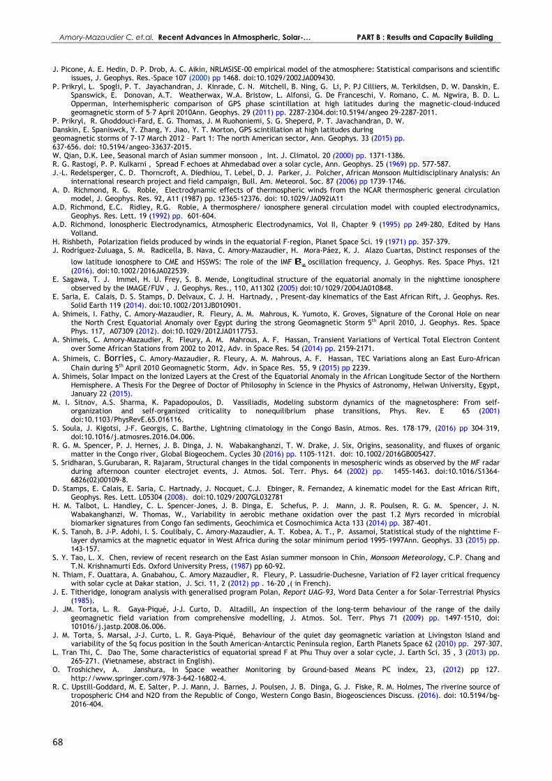
Amory-Mazaudier C. et.al. Recent Advances in Atmospheric, Solar-… PART B : Results and Capacity Building
68
J. Picone, A. E. Hedin, D. P. Drob, A. C. Aikin, NRLMSISE-00 empirical model of the atmosphere: Statistical comparisons and scientific issues, J. Geophys. Res.-Space 107 (2000) pp 1468. doi:10.1029/2002JA009430.
P. Prikryl, L. Spogli, P. T. Jayachandran, J. Kinrade, C. N. Mitchell, B. Ning, G. Li, P. PJ Cilliers, M. Terkildsen, D. W. Danskin, E. Spanswick, E. Donovan, A.T. Weatherwax, W.A. Bristow, L. Alfonsi, G. De Franceschi, V. Romano, C. M. Ngwira, B. D. L. Opperman, Interhemispheric comparison of GPS phase scintillation at high latitudes during the magnetic-cloud-induced geomagnetic storm of 5–7 April 2010Ann. Geophys. 29 (2011) pp. 2287-2304.doi:10.5194/angeo 29-2287-2011.
P. Prikryl, R. Ghoddouci-Fard, E. G. Thomas, J. M Ruohoniemi, S. G. Sheperd, P. T. Javachandran, D. W. Danskin, E. Spaniswck, Y. Zhang, Y. Jiao, Y. T. Morton, GPS scintillation at high latitudes during geomagnetic storms of 7-17 March 2012 – Part 1: The north American sector, Ann. Geophys. 33 (2015) pp. 637-656. doi: 10.5194/angeo-33637-2015. W. Qian, D.K. Lee, Seasonal march of Asian summer monsoon , Int. J. Climatol. 20 (2000) pp. 1371-1386. R. G. Rastogi, P. P. Kulkarni , Spread F echoes at Ahmedabad over a solar cycle, Ann. Geophys. 25 (1969) pp. 577-587. J.-L. Redelsperger, C. D. Thorncroft, A. Diedhiou, T. Lebel, D. J. Parker, J. Polcher, African Monsoon Multidisciplinary Analysis: An
international research project and field campaign, Bull. Am. Meteorol. Soc. 87 (2006) pp 1739–1746. A. D. Richmond, R. G. Roble, Electrodynamic effects of thermospheric winds from the NCAR thermospheric general circulation
model, J. Geophys. Res. 92, A11 (1987) pp. 12365-12376. doi: 10.1029/JA092iA11 A.D. Richmond, E.C. Ridley, R.G. Roble, A thermosphere/ ionosphere general circulation model with coupled electrodynamics,
Geophys. Res. Lett. 19 (1992) pp. 601-604. A.D. Richmond, Ionospheric Electrodynamics, Atmospheric Electrodynamics, Vol II, Chapter 9 (1995) pp 249-280, Edited by Hans
Volland. H. Rishbeth, Polarization fields produced by winds in the equatorial F-region, Planet Space Sci. 19 (1971) pp. 357-379. J. Rodríguez-Zuluaga, S. M. Radicella, B. Nava, C. Amory-Mazaudier, H. Mora-Páez, K. J. Alazo Cuartas, Distinct responses of the
low latitude ionosphere to CME and HSSWS: The role of the IMF oscillation frequency, J. Geophys. Res. Space Phys. 121 (2016). doi:10.1002/2016JA022539.
E. Sagawa, T. J. Immel, H. U. Frey, S. B. Mende, Longitudinal structure of the equatorial anomaly in the nighttime ionosphere observed by the IMAGE/FUV , J. Geophys. Res., 110, A11302 (2005) doi:10/1029/2004JA010848.
E. Saria, E. Calais, D. S. Stamps, D. Delvaux, C. J. H. Hartnady, , Present-day kinematics of the East African Rift, J. Geophys. Res. Solid Earth 119 (2014). doi:10.1002/2013JB010901.
A. Shimeis, I. Fathy, C. Amory-Mazaudier, R. Fleury, A. M. Mahrous, K. Yumoto, K. Groves, Signature of the Coronal Hole on near the North Crest Equatorial Anomaly over Egypt during the strong Geomagnetic Storm 5th April 2010, J. Geophys. Res. Space Phys. 117, A07309 (2012). doi:10.1029/2012JA0117753.
A. Shimeis, C. Amory-Mazaudier, R. Fleury, A. M. Mahrous, A. F. Hassan, Transient Variations of Vertical Total Electron Content over Some African Stations from 2002 to 2012, Adv. in Space Res. 54 (2014) pp. 2159-2171.
A. Shimeis, C. Borries, C. Amory-Mazaudier, R. Fleury, A. M. Mahrous, A. F. Hassan, TEC Variations along an East Euro-African Chain during 5th April 2010 Geomagnetic Storm, Adv. in Space Res. 55, 9 (2015) pp 2239.
A. Shimeis, Solar Impact on the Ionized Layers at the Crest of the Equatorial Anomaly in the African Longitude Sector of the Northern Hemisphere. A Thesis For the Degree of Doctor of Philosophy in Science in the Physics of Astronomy, Helwan University, Egypt, January 22 (2015).
M. I. Sitnov, A.S. Sharma, K. Papadopoulos, D. Vassiliadis, Modeling substorm dynamics of the magnetosphere: From self-organization and self-organized criticality to nonequilibrium phase transitions, Phys. Rev. E 65 (2001) doi:10.1103/PhysRevE.65.016116.
S. Soula, J. Kigotsi, J-F. Georgis, C. Barthe, Lightning climatology in the Congo Basin, Atmos. Res. 178–179, (2016) pp 304–319, doi:10.1016/j.atmosres.2016.04.006.
R. G. M. Spencer, P. J. Hernes, J. B. Dinga, J. N. Wabakanghanzi, T. W. Drake, J. Six, Origins, seasonality, and fluxes of organic matter in the Congo river, Global Biogeochem. Cycles 30 (2016) pp. 1105-1121. doi: 10.1002/2016GB005427.
S. Sridharan, S.Gurubaran, R. Rajaram, Structural changes in the tidal components in mesospheric winds as observed by the MF radar during afternoon counter electrojet events, J. Atmos. Sol. Terr. Phys. 64 (2002) pp. 1455-1463. doi:10.1016/S1364-6826(02)00109-8.
D. Stamps, E. Calais, E. Saria, C. Hartnady, J. Nocquet, C.J. Ebinger, R. Fernandez, A kinematic model for the East African Rift, Geophys. Res. Lett. L05304 (2008). doi:10.1029/2007GL032781
H. M. Talbot, L. Handley, C. L. Spencer-Jones, J. B. Dinga, E. Schefus, P. J. Mann, J. R. Poulsen, R. G. M. Spencer, J. N. Wabakanghanzi, W. Thomas, W., Variability in aerobic methane oxidation over the past 1.2 Myrs recorded in microbial biomarker signatures from Congo fan sediments, Geochimica et Cosmochimica Acta 133 (2014) pp. 387-401.
K. S. Tanoh, B. J-P. Adohi, I. S. Coulibaly, C. Amory-Mazaudier, A. T. Kobea, A. T., P. Assamoi, Statistical study of the nighttime F-layer dynamics at the magnetic equator in West Africa during the solar minimum period 1995-1997Ann. Geophys. 33 (2015) pp. 143-157.
S. Y. Tao, L. X. Chen, review of recent research on the East Asian summer monsoon in Chin, Monsoon Meteorology, C.P. Chang and T.N. Krishnamurti Eds. Oxford University Press, (1987) pp 60-92.
N. Thiam, F. Ouattara, A. Gnabahou, C. Amory Mazaudier, R. Fleury, P. Lassudrie-Duchesne, Variation of F2 layer critical frequency with solar cycle at Dakar station, J. Sci. 11, 2 (2012) pp . 16-20 ,( in French).
J. E. Titheridge, Ionogram analysis with generalised program Polan, Report UAG-93, Word Data Center a for Solar-Terrestrial Physics (1985).
J. JM. Torta, L. R. Gaya-Piqué, J-J. Curto, D. Altadill, An inspection of the long-term behaviour of the range of the daily geomagnetic field variation from comprehensive modelling, J. Atmos. Sol. Terr. Phys 71 (2009) pp. 1497-1510, doi: 101016/j.jastp.2008.06.006.
J. M. Torta, S. Marsal, J-J. Curto, L. R. Gaya-Piqué, Behaviour of the quiet day geomagnetic variation at Livingston Island and variability of the Sq focus position in the South American-Antarctic Peninsula region, Earth Planets Space 62 (2010) pp. 297-307.
L. Tran Thi, C. Dao The, Some characteristics of equatorial spread F at Phu Thuy over a solar cycle, J. Earth Sci. 35 , 3 (2013) pp. 265-271. (Vietnamese, abstract in English).
O. Troshichev, A. Janshura, In Space weather Monitoring by Ground-based Means PC index, 23, (2012) pp 127. http://www.springer.com/978-3-642-16802-4.
R. C. Upstill-Goddard, M. E. Salter, P. J. Mann, J. Barnes, J. Poulsen, J. B. Dinga, G. J. Fiske, R. M. Holmes, The riverine source of tropospheric CH4 and N2O from the Republic of Congo, Western Congo Basin, Biogeosciences Discuss. (2016). doi: 10.5194/bg-2016-404.

Sun and Geosphere, 2017; 12/ 2-Supplement 21÷69 ISSN 2367-8852
69
V. Uritsky, A. Klimas, A., D. Vassiliadis, Comparative study of dynamical critical scaling in the auroral electrojet index versus solar wind fluctuations, Geophys. Res. Lett. 28 (2001) pp. 3809-3812.
V. Uritsky, A. J. Klimas, D. Vassiliadis, Critical finite-size scaling of energy and lifetime probability distributions of auroral emissions, Geophys. Res. Lett. 33, L08102 (2006). doi:10.1029/2005GL025330.
V.M. Vasyliunas, Mathematical models of magnetospheric convection and its coupling to the ionosphere in Particles and Fields in the Magnetosphere, edited by B.M. McCormac, Springer, New York (1970) pp. 60-71.
V.M. Vasyliunas, The inter-relationship of magnetospheric processes, in Earth’s Magnetosphere Processes, edited by M. McCormac Springer, New York (1972) pp. 29-38.
M. Vázquez, J. M. Vaquero, J.J Curto, On the connection between solar activity and low latitude aurorae in the period 1715-1860, Sol. Phys. 238 , 2 (2006) pp. 405-420.
B. Wang, L. Ho, Rainy Season of the Asian-Pacific Summer, J. Climate 15 (2002) pp. 386-398. J. A. Wanliss, Fractal properties of SYM-H during quiet and active times, J.Geophys. Res. 110 (2005). doi:10.1029/2004JA010544. J. A. Wanliss, P. Dobias, Space storm as a dynamic phase transition, J. Atmos. Sol. Terr. Phys. 69 (2007) pp. 675-684. Y. Yamazaki, K. Yumoto, D. McNamara,T. Hirooka, T. Uozumi, K. Kitamura, S. Abe, A. Ikeda, Ionospheric current system during
sudden stratospheric warming events, J. Geophys. Res. 117, A03334 (2012). doi:10.1029/2011JA017453. E. Yizengaw, M. B. Moldwin, African Meridian B-field Education and Research (AMBER) Earth Moon Planet 104, 1 (2009) pp. 237-246. E. Yizengaw, E. Zesta, C.M. Biouele, M.B. Moldwin, A. Boudouridis, B. Damtie, A. Mebrahtu, F. Anad, R.F. Pfaff, M. Hartinger,
Observations of ULF wave related equatorial electrojet and density fluctuations, J. Atmos. Sol.-Terr. Phys. 103 (2013) pp 157
ISSN 1364-6826, http://dx.doi.org/10.1016/j.jastp.2013.03.015. E. Yizengaw, P. Doherty, T. Fuller-Rowell, Is space weather different over Africa, and if so, why? AGU Chapman conference report,
Space Weather 11 (2014) pp 389–391, doi:10.1002/swe.20063. W. Yuan, X. Liu, J. Xu, Q. Zhou, G. Jiang, R. Ma, FPI observations of nighttime mesospheric and thermospheric winds in China and
their comparisons with HWM07,Ann. Geophys. 31 (2013) pp. 1365-1378, doi:10.5194/angeo-31-1365-2013. X. Yue, L. Liu, W. Wan, Y. Wei, Z. Ren, Modeling the effects of secular variation of geomagnetic filed orientation on the
ionospheric long term trend over the past century, J. Geophys. Res. 113, A10301 (2008). doi:10.1029/2007JAO12995. K. Z. Zaka, A. T. Kobea, P. Assamoi, O. K. Obrou, V. Doumbia, K. Boka, B. J.-P. Adohi, N. M. Mene, Latitudinal profile of the
ionospheric disturbance dynamo magnetic signature: comparison with the DP2 magnetic disturbance, Ann. Geophys. 27 (2009) pp. 3523-3536.
K. Z. Zaka, A.T. Kobea, V. Doumbia, A. D. Richmond, A. Maute, A., N. M. Mene, O. K. Obrou, P. Assamoi, K. Boka, B. J-P. Adohi, C. Amory-Mazaudier, Simulation of electric field and current during the June 11, 1993, disturbance dynamo event: comparison with the observations, J. Geophys. Res. 115, A11307 (2010). doi:10.1029/2010JA015417.
N. Zaourar, R. Mebarki, L. Briqueu, M. Mandea, M. Hamoudi, Wavelet analysis applied to InterMagnet data: Singularity detections related to geomagnetic storms, NRIAG J. Geophys., Special Issue (2009) pp. 295-309.
N. Zaourar, M. Hamoudi, M. Mandea, G. Balasis, M. Holschneider, Wavelet-based multiscale analysis of geomagnetic disturbance,Earth Planets Space 65 (2013a) pp. 1525-1540.
N. Zaourar, M. Hamoudi, M. Mandea, M. Holschneider , Fractal dynamics of geomagnetic storms ,Arabian J. Geosci. June, 6, 6 (2013b) pp. 1693-1702.
N. Zaourar, C. Amory-Mazaudier, R. Fleury, Hemispheric asymmetries in the ionosphere response observed during the high-speed solar wind streams of the 24-28 August 2010, Adv. Space Res. (2017). doi.org/10.1016/j.asr.2017.01.048.
J.-L. Zerbo, C. Amory-Mazaudier, F. Ouattara, J.D. Richardson, Solar wind and geomagnetism, toward a standard classification 1868-2009, Ann. Geophys. 30 (2012a) pp. 421-426.
J.-L. Zerbo, C. Amory-Mazaudier, F. Ouattara, Geomagnetism during solar cycle 23, J. of Advanced Res. 4 , 3 (2012b) pp 265,
doi:10.1016/j.jare.2013.08.010 J.-L. Zerbo, F. Ouattara, E. Nanéma, Solar activity and Meteorological fluctuations in West Africa: Temperatures and Pluviometry in
Burkina Faso, 1970-2012, International J. Astron. and Astrophys. 3 (2013a ) pp. 408-411. doi: 10.4236/ijaa.2013.34048. J.-L Zerbo, F. Ouattara, C. Amory Mazaudier, J-P. Legrand, J. D. Richardson, Solar activity, Solar wind and Geomagnetism
signatures, Atmos. and Climate Sci. 6 (2013b) pp. 610-617. J.-L. Zerbo, C. Amory-Mazaudier, F. Ouattara, Solar wind fluctuations and solar activity long-term swing: 1963-2012, Proc. of
International Astronomical Union, (2013c) pp 443. Cambridge Journals. doi:10.1017/S1743921313011617 J.-L. Zerbo, J.D. Richardson, The Solar wind during current and past solar minima and maxima, J. Geophys. Res. Space Physics 120,
12 (2015) pp 10250. Y. Zhang, T. Lib, B. Wang, G. Wu, Onset of the Summer Monsoon over the Indochina Peninsula: climatology and interannual
variations, J. Climate 15 (2002) pp. 3206-3221. A. W. Zhaohui, J. B. Dinga, J. Paul, P. J. Mann, K. Hoering, J. Poulsen, R.G. M. Spencer, R. M. Holmes, Inorganic carbon speciation
and fluxes in the Congo river, Geophys. Res. Lett. 40 (2013) pp. 1-6. doi:10.1002/grl.50160. C. Zoundi, F. Ouattara, R. Fleury, C. Amory-Mazaudier, P. Lassudrie-Duchesne, Seasonal TEC variability in West Africa Equatorial
Anomaly Region, European J. Scientific Res. 77, 3 (2012) pp. 309-319. C. Zoundi, F. Ouattara, E. Nanema, C. Fleury , CODG TEC variation during solar maximum and minimum over Niamey, European
Scientific Journal 9, 27 (2013) pp. 74-80.