real-time control of a magnetic levitation system for time

Real-time Control of a Magnetic LevitationSystem for Time-varying Reference Tracking

Eduardo Giraldo

Abstract—In this work, a design and implementation of amodified PID for tracking time-varying references are designed.The modified PID structure allows the reduction of the zerosadded by the classical PID structure. The design of thecontroller is performed by considering time features such assettling time and maximum overshoot. The proposed controlleris implemented and evaluated over a Hardware-in-the-Loopstructure for real-time control performance. The controller isdesigned around an operational point and is evaluated for initialconditions, constant references, and time-varying references interms of settling time and maximum overshoot. As a result,the modified PID structure shows advantages over the classicalPID structure in terms of settling-time, maximum overshoot,and fidelity to the designed features.

Index Terms—Real-time, PID control, Magnetic Levitation,Time-varying reference.

I. INTRODUCTION

THE design of PID controllers over nonlinear systems isusually performed by using the transfer function H(s)

of the system computed by a linear approximation of thenonlinear system around an operational point [1]. Severalcontrollers can also be applied over nonlinear systems,such as variable structure controllers [2], adaptive robustcontrollers [3] or intelligent controller [4]. It is worth notingthat a key factor in the design of controllers over realsystems is the evaluation of the controller over simulatedand real prototypes [5]. These prototypes are usuallybuild-up by using Hardware-In-the-Loop (HIL) strategiesor Software-In-the-Loop (SIL) structures, being the HILstructure the most common implementation to evaluate theeffectiveness of the controller [6].

The common equation for a PID controller is defined as

u(t) = Kpe(t) +Ki

∫e(τ)dτ +Kd

de

dt(1)

being Kp, Ki and Kd, the controller parameters, and e(t)the tracking error computed as

e(t) = r(t)− y(t) (2)

being r(t) the reference of desired output signal and y(t) theoutput of the system to be controlled [7].

The transfer function of the error-based PID controllerof (1), defined as C(s) is obtained by applying the Laplacetransform over (1) as:

C(s) = Kp +Ki

s+Kds (3)

Manuscript received March 1, 2021; revised July 27, 2021. This workwas carried out under the funding of the Universidad Tecnologica dePereira, Vicerrectorıa de Investigacion, Innovacion y Extension. Researchproject: 6-20-7 “Estimacion Dinamica de estados en sistemas multivariablesacoplados a gran escala”.

Eduardo Giraldo is a Full Professor at the Department of ElectricalEngineering, Universidad Tecnologica de Pereira, Pereira, Colombia.Research group in Automatic Control. E-mail: [email protected].

being U(s) = C(s)E(s) and considering that the trackingerror is computed by

E(s) = R(s)− Y (s) (4)

where the linearized plant to be controlled H(s) around anoperational point is defined as:

Y (s) = H(s)U(s) (5)

The resulting block diagram of the closed-loop systemconsidering (3), (5) and (4) is presented in Fig. 1.

Fig. 1. Closed Loop controller

The success of the controller is highly dependant of thevariability of the nonlinear function around the operationalpoint where the system is operating [8]. The closed-looptransfer function can be obtained from the block diagramof Fig. 1, as follows:

Y (s) = HCLR(s) (6)

being HCL defined as

HCL =H(s)C(s)

1 +H(s)C(s)(7)

Two design criteria are usually applied to design thecontroller [9]. The first one is based on the closed-loopcharacteristic equation pLC(s) which is the denominatorof the closed-loop transfer function. This design criteriaconsiders a desired equation for the closed-loop dynamicsas pd(s) where the following relation is defined

pCL(s) = pd(s) (8)

The second criteria considers the steady-state error ess byapplying the Final Value Theorem computed as follows

ess = limt→∞

e(t) = lims→0

sE(s) (9)

This design criteria considers that the absolute value of thesteady-state error must achieve the following condition

|ess| ≤ ε (10)

being ε > 0 a threshold defined as the maximum permissibleerror for steady-state.

A methodology to design a PID controller for nonlinearsystems around an operational point is presented in this

IAENG International Journal of Applied Mathematics, 51:3, IJAM_51_3_39

Volume 51, Issue 3: September 2021

______________________________________________________________________________________

work. The methodology is obtained by combining (8)and (10) to design the controller, which results in a PIDwith time-varying tracking capabilities. A modified structureof the PID is used to reduce the effect of the zerosadded by the controller structure. The proposed approachis validated by using a Magnetic Levitation nonlinearsystem around an operational point. The tracking capabilitiesare evaluated for initial conditions, constant references,and time-varying references. A HIL implementation ofthe Magnetic Levitation is used to evaluate the controllerperformance over a real system. This paper is organized asfollows: section II describes the mathematical methods formodeling the magnetic levitation system and PID design.In section III the discrete equations used for real-timeimplementation of the controller and the HIL model ofthe magnetic levitation system are presented, and finally, insection IV the results and discussion are shown.

II. MATHEMATICAL MODEL

Consider the Magnetic Levitation model of Fig. 2 withcurrent u(t) as an input, and output y(t) the displacement ofmass M .

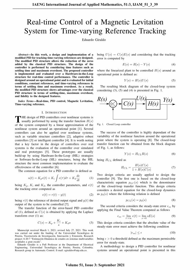
Fig. 2. Magnetic Levitation system

The system of Fig. 2 can be modeled by the followingdynamical equation

Mg −Ku(t)

y(t)= My (11)

By considering the operational point y0 a constant, anequilibrium equation can be obtained

Mg −Ku0

y0= 0 (12)

where u0 is obtained as

u0 =Mgy0

K(13)

The linear approximation of (11) by using Taylor seriesapproximation is obtained as

−Ky0

M∆u(t) +

Ku0

My20

∆y(t) = ∆y (14)

By defining the parameters of the Magnetic Levitation systemof (11) as M = 0.05, K = 1, g = 9.8 and y0 = 0.01, thefollowing linear equation is obtained:

−2000∆u(t) + 980∆y(t) = ∆y (15)

By applying the Laplace transform over (15) the transferfunction of the Magnetic Levitation system of Fig. 2 isobtained

∆Y (s) =−2000

s2 − 980∆U(s) (16)

In Fig. 3, is presented the resulting linear closed-loopblock diagram.

Fig. 3. Linear closed-loop block diagram

The steady-state error by using the Final Value theoremaround an operational point is re-defined for the linear modelas follows:

∆ess = lims→0

s∆E(s) (17)

where ∆E(s) is obtained from the block diagram of Fig. 3as follows:

∆E(s) =s3 − 980s

s3 − 2000Kds2 − (2000Kp + 980)s− 2000Ki

∆R(s) (18)

where the closed-loop characteristic equation pCL(s) is

pCL(s) = s3 − 2000Kds2 − (2000Kp+ 980)s− 2000Ki

(19)

The first criteria for desired poles suggest that thedynamical behaviour of the closed-loop system must bedetermined by the following closed-loop complex poles:

s1,2 = −2± j√

2

However, since pCL(s) is a third order equation, anadditional pole is required for the desired closed-loopequation pd(s). Therefore, the pd(s) is defined as

pd(s) = (s+ 2 + j√

2)(s+ 2− j√

2)(s+ p) (20)

being s = −p with p > 0, the additional closed-loop pole.From (20), the pd(s) can be obtained as

pd(s) = s3 + (4 + p)s2 + (4p+ 6)s+ 6p (21)

By defining pd(s) = pCL(s) the following relationshipscan be obtained

−2000Ki = 6p (22)−(2000Kp + 980) = 4p+ 6 (23)

−2000Kd = 4 + p (24)

where is remarkable that, since p > 0 then Ki must benegative. It is noticeable the equations (22), (23) and (24)describe a system of three equations and four unknownquantities. In order to obtain an additional constraint andsolve the system, the second criteria for steady-state error isused.

The second criteria considers the steady-state error of (17),where ∆ess is equal to zero for ∆R(s) of type impulseand step. For time-varying references ∆R(s) of type ramp,



______________________________________________________________________________________

∆ess is not equal to zero. For this case, the steady-state errorof (17) around and operational point is defined as

∆ess =980

2000Ki(25)

where a ∆R(s) = 1s2 is used. By considering an ε = 0.05

for the second criteria, the resulting constraint is

|∆ess| ≤ 0.05 (26)

and therefore

|Ki| ≥ 98 (27)

By choosing Ki = −100 the resulting p is p = 2000006

and therefore, Kp and Kd are

Kp = −67.15 (28)Kd = −16.66 (29)

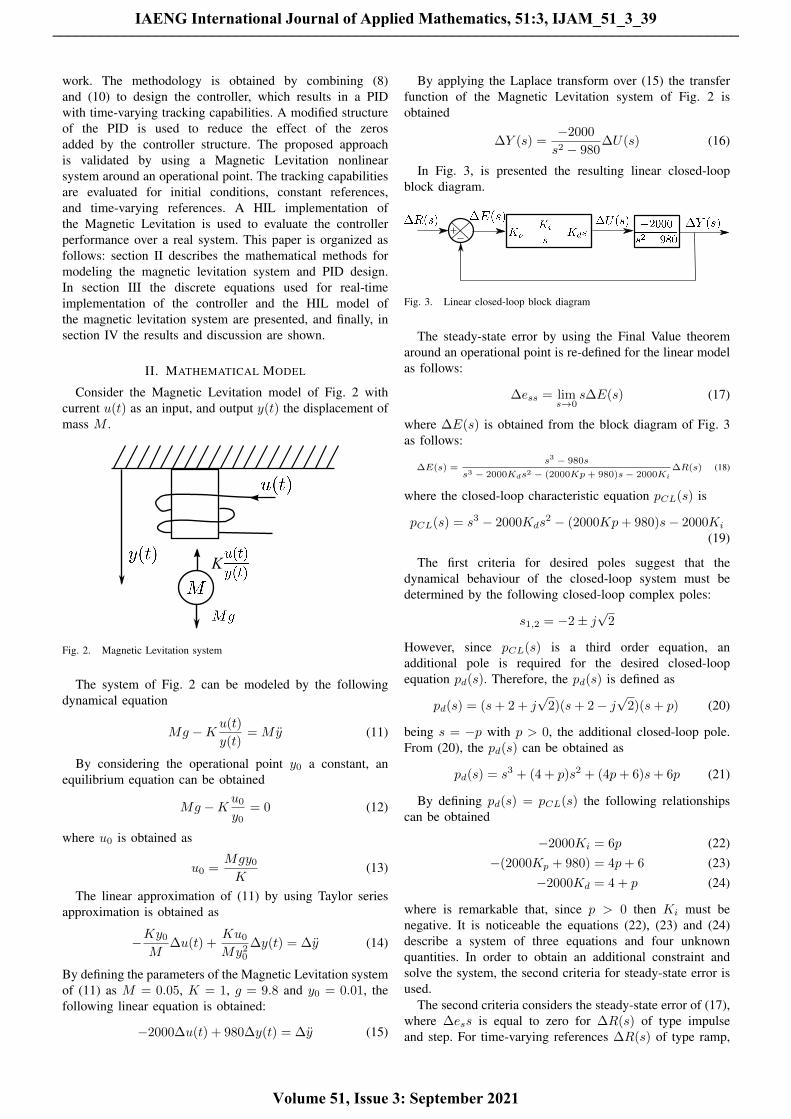
It is worth noting that the dominant response of theclosed-loop system is approximated by the transfer function

Y (s) ≈ ω2n

s2 + 2ρωns+ ω2n

R(s) (30)

being the damping coefficient ρ = 0.816 and ωn = 2.45,which is presented in Fig. 4.

Fig. 4. Dominant response of the closed-loop system

It can be seen that the maximum overshot is around 1.18%of the unitary step, and the settling time is around 2 seconds.

The resulting closed-loop transfer function is given by

∆Y (s) =−2000(Kds

2 + Kps + Ki)

s3 − 2000Kds2 − (2000Kp + 980)s− 2000Ki

∆R(s) (31)

It is worth noting that the closed-loop transfer function hastwo zeros related directly to the controller, in comparisonwith the system that has no zeros. This phenomenon is dueto the structure of the PID controller, where the derivativeand proportional actions are related directly to the error. Ifthe structure of Fig. 3 is modified as shown in Fig. 5 theresulting closed-loop has no zeros.

Fig. 5. Linear closed-loop with modified PID structure

By considering Fig. 5 the resulting closed-loop transferfunction is now given by

∆Y (s) =−2000Ki

s3 − 2000Kds2 − (2000Kp + 980)s− 2000Ki

∆R(s) (32)

where the closed-loop characteristic equation is hold, andwhere the transfer function for the error is now defined as

∆E(s) =s3 − 2000Kds

2 − (2000Kp + 980)s

s3 − 2000Kds2 − (2000Kp + 980)s− 2000Ki

∆R(s) (33)

which has the same dynamics but for the selected valuesof the controller, the steady-state error for a ramp referencesignal, is computed as

|∆ess| = 0.66 (34)

Therefore, in order to reduce the steady-state error, andaccording to the stability criteria, the controller parametersmust be recalculated. For time-varying references ∆R(s) oftype ramp, ∆ess is not equal to zero. For this case, thesteady-state error of (17) around and operational point isdefined as

∆ess =2000Kp + 980

2000Ki(35)

where a ∆R(s) = 1s2 is used. By considering an ε = 0.05

for the second criteria, the resulting constraint is

|∆ess| ≤ 0.05 (36)

III. REAL-TIME CONTROL EVALUATION

The real time implementation of the magnetic levitationsystem of (11) is performed by an approximation of thenonlinear model by using the backwards operator. Theresulting nonlinear difference equation is defined as

y[k] = gh2 − Kh2u[k − 2]

My[k − 2]+ 2y[k − 1]− y[k − 2] (37)

The discrete implementation of the PID controller in itsclassical or modified structure is based on the approximationby backward differences of derivative and integrativeoperators. The classical structure of the PID is implementedby using the following set of difference equations:

ei[k] = ei[k − 1] + he[k] (38)

ed[k] =e[k]− e[k − 1]

h(39)

u[k] = Kpe[k] +Kded[k] +Kiei[k] (40)

being ei[k] the integral of the error e[k] and ed[k] thederivative of the error e[k], and h the sample time, wherethe error e[k] = r[k]− y[k].

The block diagram of the Hardware-In-the-Loop (HIL)implementation of the classical PID controller over aMagnetic Levitation (MagLev) model is presented in Fig. 6.



______________________________________________________________________________________

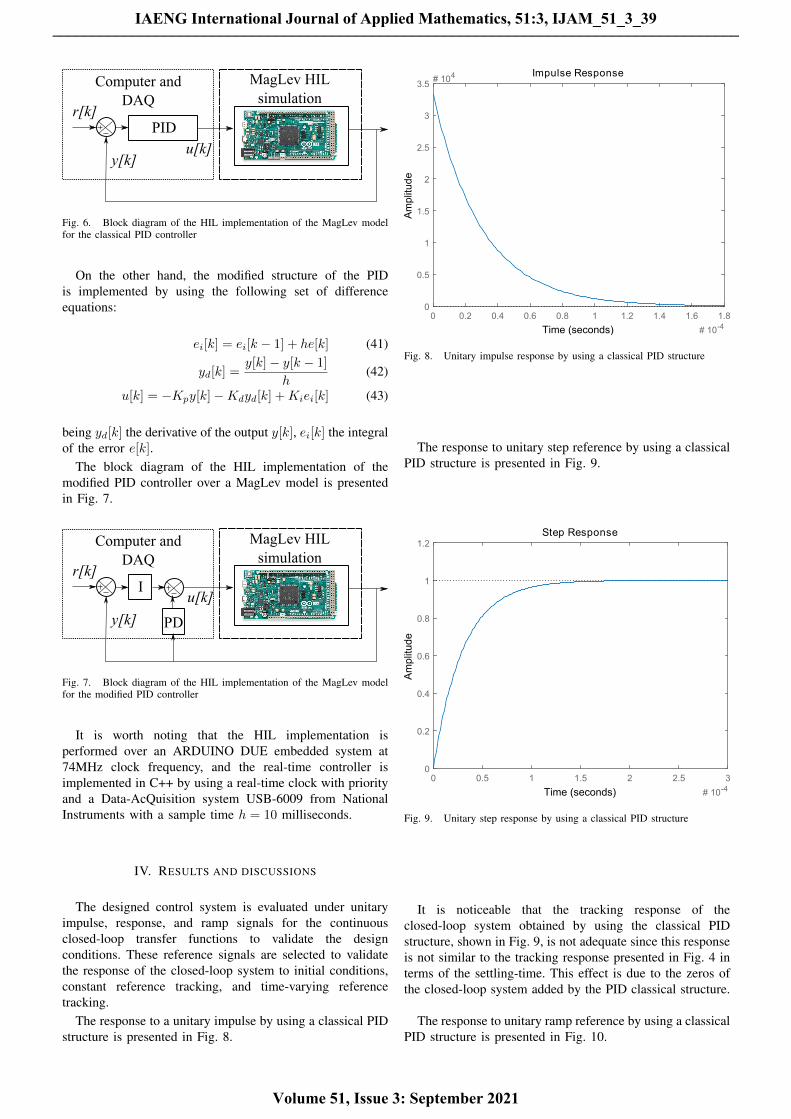
Fig. 6. Block diagram of the HIL implementation of the MagLev modelfor the classical PID controller

On the other hand, the modified structure of the PIDis implemented by using the following set of differenceequations:

ei[k] = ei[k − 1] + he[k] (41)

yd[k] =y[k]− y[k − 1]

h(42)

u[k] = −Kpy[k]−Kdyd[k] +Kiei[k] (43)

being yd[k] the derivative of the output y[k], ei[k] the integralof the error e[k].

The block diagram of the HIL implementation of themodified PID controller over a MagLev model is presentedin Fig. 7.

Fig. 7. Block diagram of the HIL implementation of the MagLev modelfor the modified PID controller

It is worth noting that the HIL implementation isperformed over an ARDUINO DUE embedded system at74MHz clock frequency, and the real-time controller isimplemented in C++ by using a real-time clock with priorityand a Data-AcQuisition system USB-6009 from NationalInstruments with a sample time h = 10 milliseconds.

IV. RESULTS AND DISCUSSIONS

The designed control system is evaluated under unitaryimpulse, response, and ramp signals for the continuousclosed-loop transfer functions to validate the designconditions. These reference signals are selected to validatethe response of the closed-loop system to initial conditions,constant reference tracking, and time-varying referencetracking.

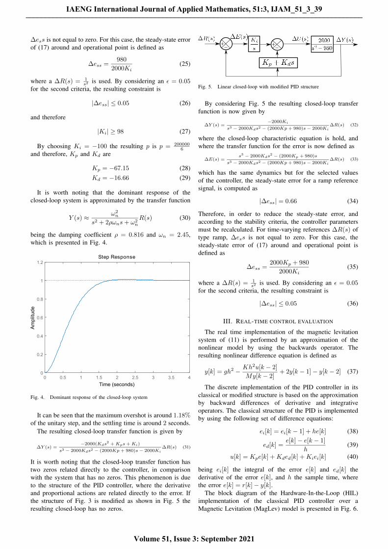
The response to a unitary impulse by using a classical PIDstructure is presented in Fig. 8.

Fig. 8. Unitary impulse response by using a classical PID structure

The response to unitary step reference by using a classicalPID structure is presented in Fig. 9.

Fig. 9. Unitary step response by using a classical PID structure

It is noticeable that the tracking response of theclosed-loop system obtained by using the classical PIDstructure, shown in Fig. 9, is not adequate since this responseis not similar to the tracking response presented in Fig. 4 interms of the settling-time. This effect is due to the zeros ofthe closed-loop system added by the PID classical structure.

The response to unitary ramp reference by using a classicalPID structure is presented in Fig. 10.



______________________________________________________________________________________

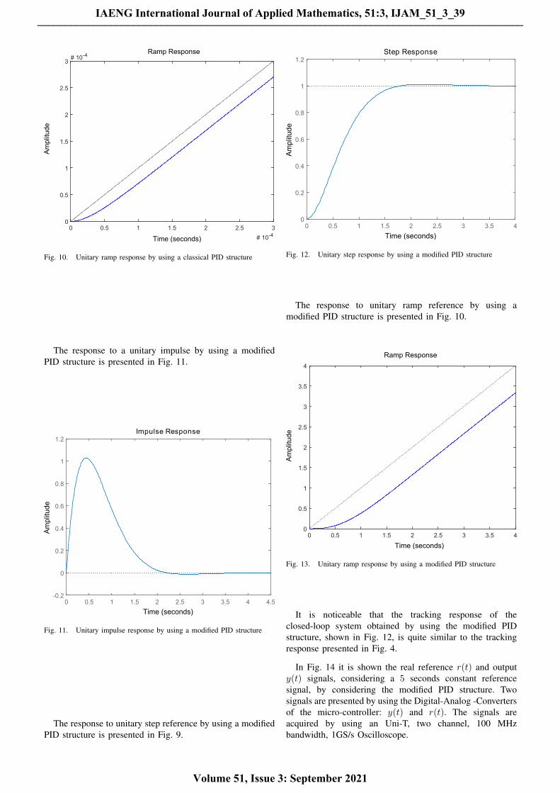
Fig. 10. Unitary ramp response by using a classical PID structure

The response to a unitary impulse by using a modifiedPID structure is presented in Fig. 11.

Fig. 11. Unitary impulse response by using a modified PID structure

The response to unitary step reference by using a modifiedPID structure is presented in Fig. 9.

Fig. 12. Unitary step response by using a modified PID structure

The response to unitary ramp reference by using amodified PID structure is presented in Fig. 10.

Fig. 13. Unitary ramp response by using a modified PID structure

It is noticeable that the tracking response of theclosed-loop system obtained by using the modified PIDstructure, shown in Fig. 12, is quite similar to the trackingresponse presented in Fig. 4.

In Fig. 14 it is shown the real reference r(t) and outputy(t) signals, considering a 5 seconds constant referencesignal, by considering the modified PID structure. Twosignals are presented by using the Digital-Analog -Convertersof the micro-controller: y(t) and r(t). The signals areacquired by using an Uni-T, two channel, 100 MHzbandwidth, 1GS/s Oscilloscope.



______________________________________________________________________________________

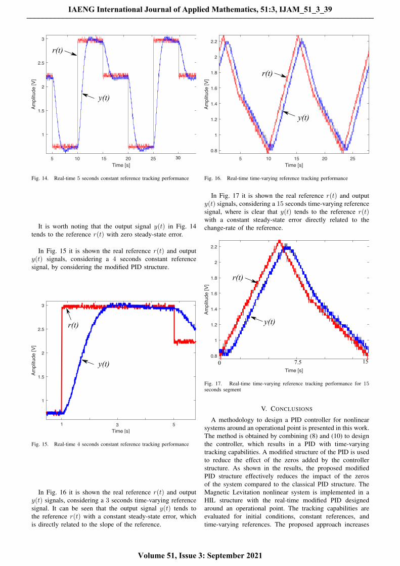
Fig. 14. Real-time 5 seconds constant reference tracking performance

It is worth noting that the output signal y(t) in Fig. 14tends to the reference r(t) with zero steady-state error.

In Fig. 15 it is shown the real reference r(t) and outputy(t) signals, considering a 4 seconds constant referencesignal, by considering the modified PID structure.

Fig. 15. Real-time 4 seconds constant reference tracking performance

In Fig. 16 it is shown the real reference r(t) and outputy(t) signals, considering a 3 seconds time-varying referencesignal. It can be seen that the output signal y(t) tends tothe reference r(t) with a constant steady-state error, whichis directly related to the slope of the reference.

Fig. 16. Real-time time-varying reference tracking performance

In Fig. 17 it is shown the real reference r(t) and outputy(t) signals, considering a 15 seconds time-varying referencesignal, where is clear that y(t) tends to the reference r(t)with a constant steady-state error directly related to thechange-rate of the reference.

Fig. 17. Real-time time-varying reference tracking performance for 15seconds segment

V. CONCLUSIONS

A methodology to design a PID controller for nonlinearsystems around an operational point is presented in this work.The method is obtained by combining (8) and (10) to designthe controller, which results in a PID with time-varyingtracking capabilities. A modified structure of the PID is usedto reduce the effect of the zeros added by the controllerstructure. As shown in the results, the proposed modifiedPID structure effectively reduces the impact of the zerosof the system compared to the classical PID structure. TheMagnetic Levitation nonlinear system is implemented in aHIL structure with the real-time modified PID designedaround an operational point. The tracking capabilities areevaluated for initial conditions, constant references, andtime-varying references. The proposed approach increases



______________________________________________________________________________________

the performance of the classical control approach in termsof design fidelity for settling-time and maximum overshoot.

REFERENCES

[1] K. J. Astrom and T. Hagglund, Advanced PID control. ISA, 2006.[2] F. Osorio-Arteaga, D. Giraldo-Buitrago, and E. Giraldo, “Sliding mode

control applied to mimo systems,” Engineering Letters, vol. 27, no. 4,pp. 802–806, 2019.

[3] F. Osorio-Arteaga, J. J. Marulanda-Durango, and E. Giraldo, “Robustmultivariable adaptive control of time-varying systems,” IAENGInternational Journal of Computer Science, vol. 47, no. 4, pp. 605–612,2020.

[4] C. D. Molina-Machado and E. Giraldo, “Bio-inspired control basedon a cerebellum model applied to a multivariable nonlinear system,”Engineering Letters, vol. 28, no. 2, pp. 464–469, 2020.

[5] T. Dohmke and H. Gollee, “Test-driven development of a pid controller,”IEEE Software, vol. 24, no. 3, pp. 44–50, 2007.

[6] A. Samiee, N. Tiefnig, J. P. Sahu, M. Wagner, A. Baumgartner, andL. Juhasz, “Model-driven-engineering in education,” in 2018 18thInternational Conference on Mechatronics - Mechatronika (ME), 2018,pp. 1–6.

[7] D. E. Davidson and J. Chen, “Classical control revisited - re-examiningthe basics in the field,” IEEE Control Systems Magazine, vol. 27, no. 1,pp. 20–21, 2007.

[8] J. S. Velez-Ramirez, L. A. Rios-Norena, and E. Giraldo, “Buckconverter current and voltage control by exact feedback linearizationwith integral action,” Engineering Letters, vol. 29, no. 1, pp. 168–176,2021.

[9] F. Golnaraghi and B. C. Kuo, Automatic Control Systems, 9th ed. USA:Wiley, 2017.



______________________________________________________________________________________

real-time control of a magnetic levitation system for time

Documents