real options theory and practice - northwestern...
TRANSCRIPT
1
INFORMS Practice Meeting, Montreal, May 2002
Real Options Theory and Practice
John R. BirgeNorthwestern University
INFORMS Practice Meeting, Montreal, May 2002
Outline
• Planning questions• Problems with traditional analyses:
examples• Real-option structure• Assumptions and differences from financial
options• Resolving inconsistencies• Conclusions
2
INFORMS Practice Meeting, Montreal, May 2002
Investment Situation: Automotive Company
• Goal: • Decide on coordinated production, distribution
capacity and vendor contracts for multiple models in multiple markets (e.g., NA, Eur, LA, Asia)
• Traditional approach• Forecast demand for each model/market• Forecast costs• Obtain piece rates and proposals• Construct cash flows and discount
! Optimize for a single-point forecast
INFORMS Practice Meeting, Montreal, May 2002
Planning Questions?
• Start product in production or not? When?• What to produce in-house or outside?• How much capacity to install?• What contracts to make outside?• External factors: economy, competitors, suppliers,
customers, legal, political, environmental• Where to start?
– Build a model
3
INFORMS Practice Meeting, Montreal, May 2002
Traditional Model• Focus on:
• Cost orientation (not revenue management)• Single program (model, product)• NPV• Piece rates
• Result: support of traditional, fixed designs, little flexibility, little ability to change, immediate investment or no investment
INFORMS Practice Meeting, Montreal, May 2002
Trends Limiting Traditional Analysis
• Market changes• Former competition:
• Cost• Quality
• New competition:• Customization• Responsiveness
4
INFORMS Practice Meeting, Montreal, May 2002
Limitations of Traditional Methodsfor New Trends
• Myopic - ignoring long-term effects• Often missing time value of cash flow• Excluding potential synergies• Ignoring uncertainty effects• Not capturing option value of delay,
scalability, and agility (changing product mix)
• Mis-calculate time-value of cash flow
INFORMS Practice Meeting, Montreal, May 2002
Outline• Planning questions• Problems with traditional analyses: examples
• Value to delay• Scalability• Reusability• Agility
• Real-option structure• Assumptions and differences from financial
options• Resolving inconsistencies• Conclusions
5
INFORMS Practice Meeting, Montreal, May 2002
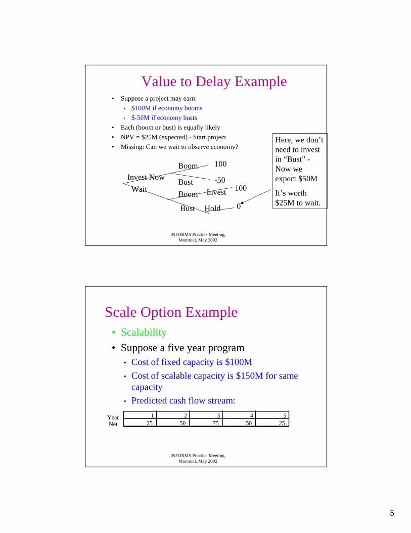
Value to Delay Example• Suppose a project may earn:
• $100M if economy booms• $-50M if economy busts
• Each (boom or bust) is equally likely• NPV = $25M (expected) - Start project• Missing: Can we wait to observe economy?
Invest NowWait
100
-50100
Boom
BustBoom
Bust
Invest
Hold 0
Here, we don’t need to invest in “Bust” -Now we expect $50M
It’s worth $25M to wait.
INFORMS Practice Meeting, Montreal, May 2002
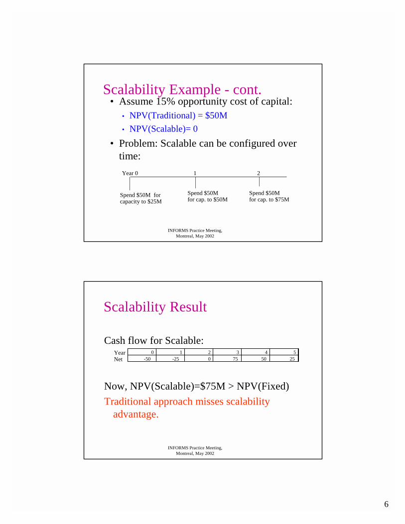
Scale Option Example• Scalability• Suppose a five year program
• Cost of fixed capacity is $100M• Cost of scalable capacity is $150M for same
capacity • Predicted cash flow stream:
1 2 3 4 525 50 75 50 25
YearNet
6
INFORMS Practice Meeting, Montreal, May 2002
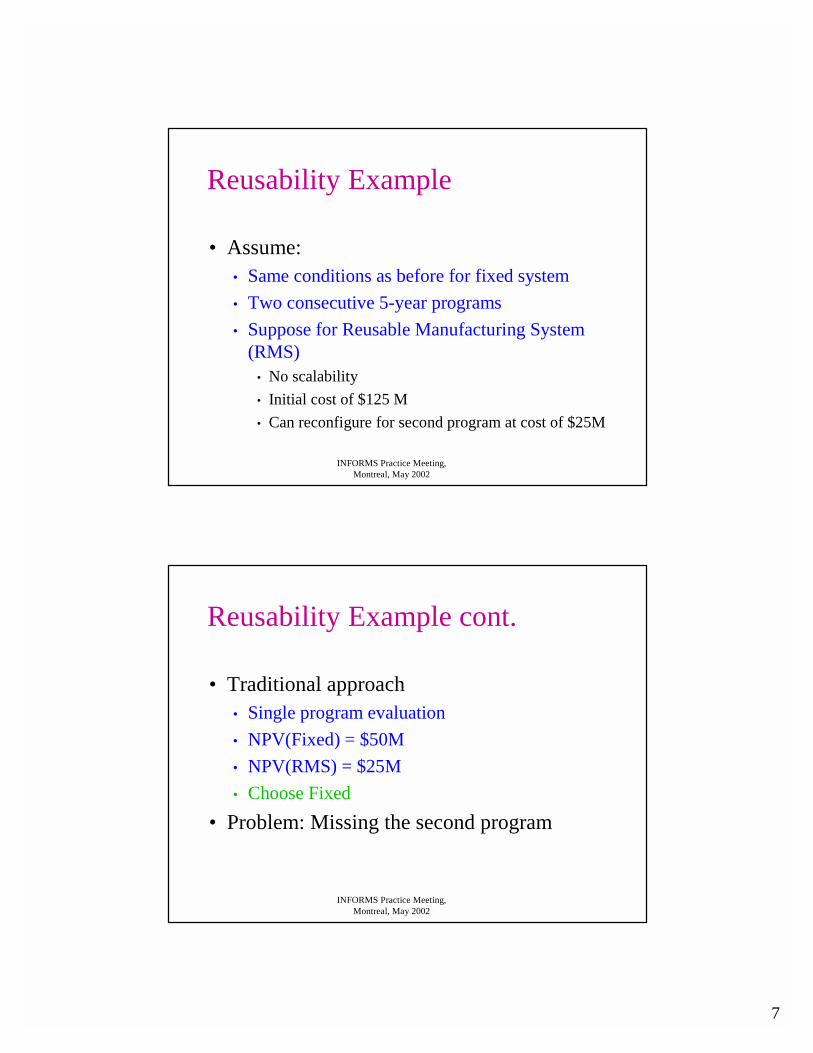
Scalability Example - cont.• Assume 15% opportunity cost of capital:
• NPV(Traditional) = $50M• NPV(Scalable)= 0
• Problem: Scalable can be configured over time:Year 0 1 2
Spend $50M forcapacity to $25M
Spend $50Mfor cap. to $50M
Spend $50Mfor cap. to $75M
INFORMS Practice Meeting, Montreal, May 2002
Scalability Result
Cash flow for Scalable:
Now, NPV(Scalable)=$75M > NPV(Fixed)Traditional approach misses scalability
advantage.
0 1 2 3 4 5-50 -25 0 75 50 25
YearNet
7
INFORMS Practice Meeting, Montreal, May 2002
Reusability Example
• Assume:• Same conditions as before for fixed system• Two consecutive 5-year programs• Suppose for Reusable Manufacturing System
(RMS)• No scalability• Initial cost of $125 M• Can reconfigure for second program at cost of $25M
INFORMS Practice Meeting, Montreal, May 2002
Reusability Example cont.
• Traditional approach• Single program evaluation• NPV(Fixed) = $50M• NPV(RMS) = $25M • Choose Fixed
• Problem: Missing the second program
8
INFORMS Practice Meeting, Montreal, May 2002
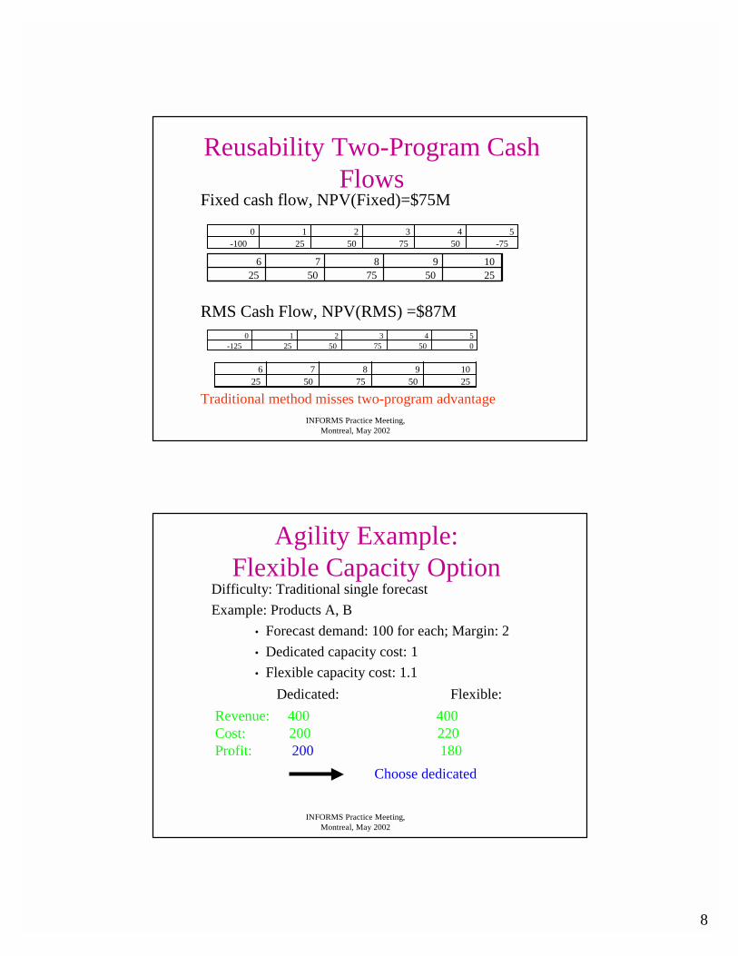
Reusability Two-Program Cash Flows
Fixed cash flow, NPV(Fixed)=$75M
RMS Cash Flow, NPV(RMS) =$87M
Traditional method misses two-program advantage
0 1 2 3 4 5-100 25 50 75 50 -75
6 7 8 9 1025 50 75 50 25
0 1 2 3 4 5-125 25 50 75 50 0
6 7 8 9 1025 50 75 50 25
INFORMS Practice Meeting, Montreal, May 2002
Difficulty: Traditional single forecastExample: Products A, B
• Forecast demand: 100 for each; Margin: 2• Dedicated capacity cost: 1• Flexible capacity cost: 1.1
Dedicated: Flexible:Revenue: 400 400Cost: 200 220Profit: 200 180
Choose dedicated
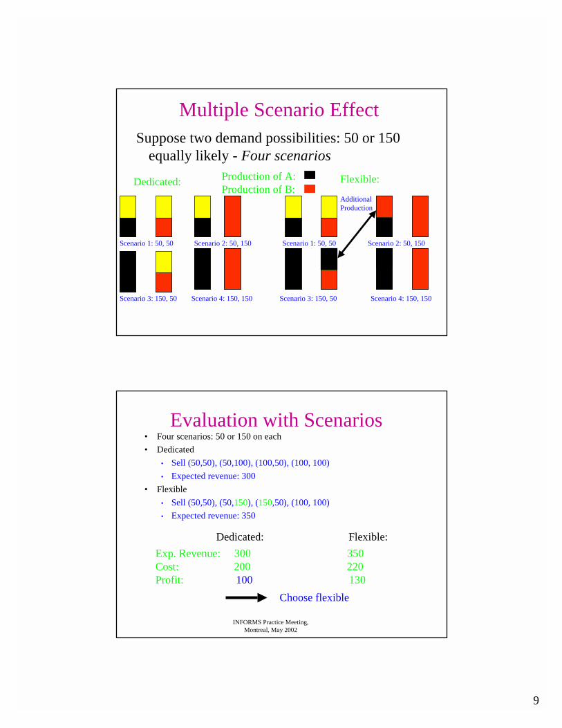
Agility Example:Flexible Capacity Option
9
Suppose two demand possibilities: 50 or 150 equally likely - Four scenarios
Dedicated: Flexible:Production of A: Production of B:
Scenario 1: 50, 50 Scenario 1: 50, 50Scenario 2: 50, 150 Scenario 2: 50, 150
Scenario 3: 150, 50 Scenario 4: 150, 150 Scenario 3: 150, 50 Scenario 4: 150, 150
AdditionalProduction
Multiple Scenario Effect
INFORMS Practice Meeting, Montreal, May 2002
• Four scenarios: 50 or 150 on each• Dedicated
• Sell (50,50), (50,100), (100,50), (100, 100)• Expected revenue: 300
• Flexible• Sell (50,50), (50,150), (150,50), (100, 100)• Expected revenue: 350
Dedicated: Flexible:Exp. Revenue: 300 350Cost: 200 220Profit: 100 130
Choose flexible
Evaluation with Scenarios
10
INFORMS Practice Meeting, Montreal, May 2002
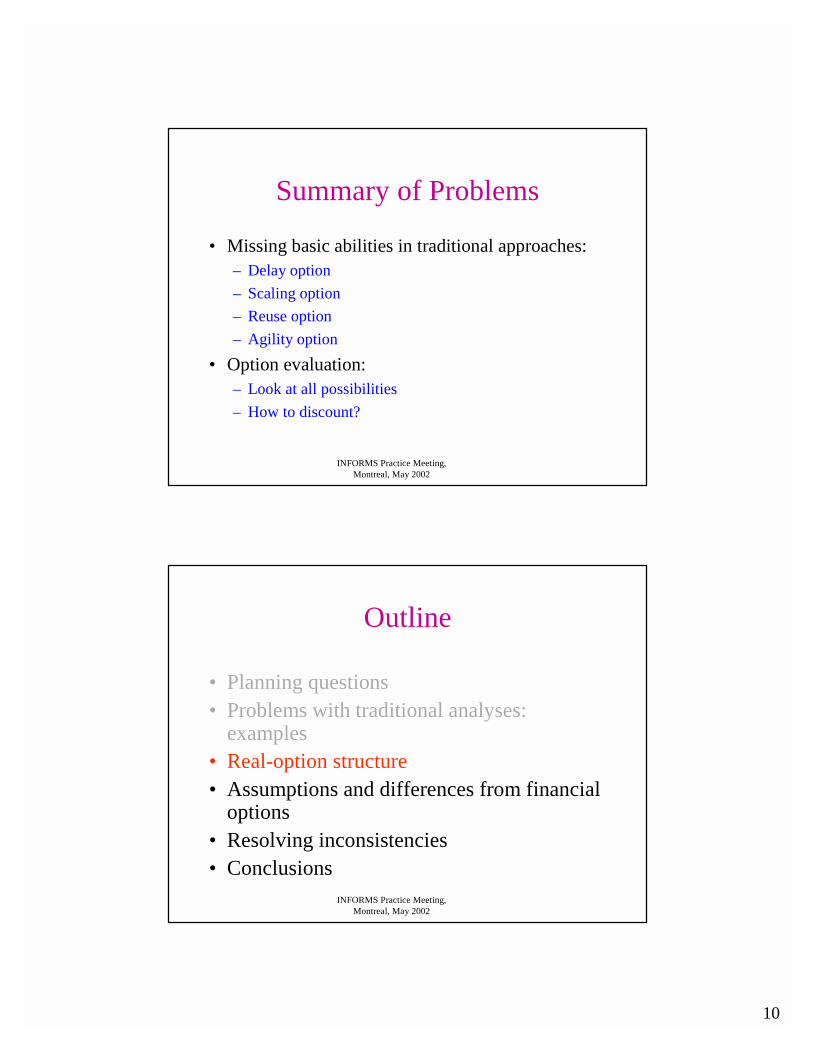
Summary of Problems
• Missing basic abilities in traditional approaches:– Delay option – Scaling option– Reuse option – Agility option
• Option evaluation: – Look at all possibilities– How to discount?
INFORMS Practice Meeting, Montreal, May 2002
Outline
• Planning questions• Problems with traditional analyses:
examples• Real-option structure• Assumptions and differences from financial
options• Resolving inconsistencies• Conclusions
11
INFORMS Practice Meeting, Montreal, May 2002
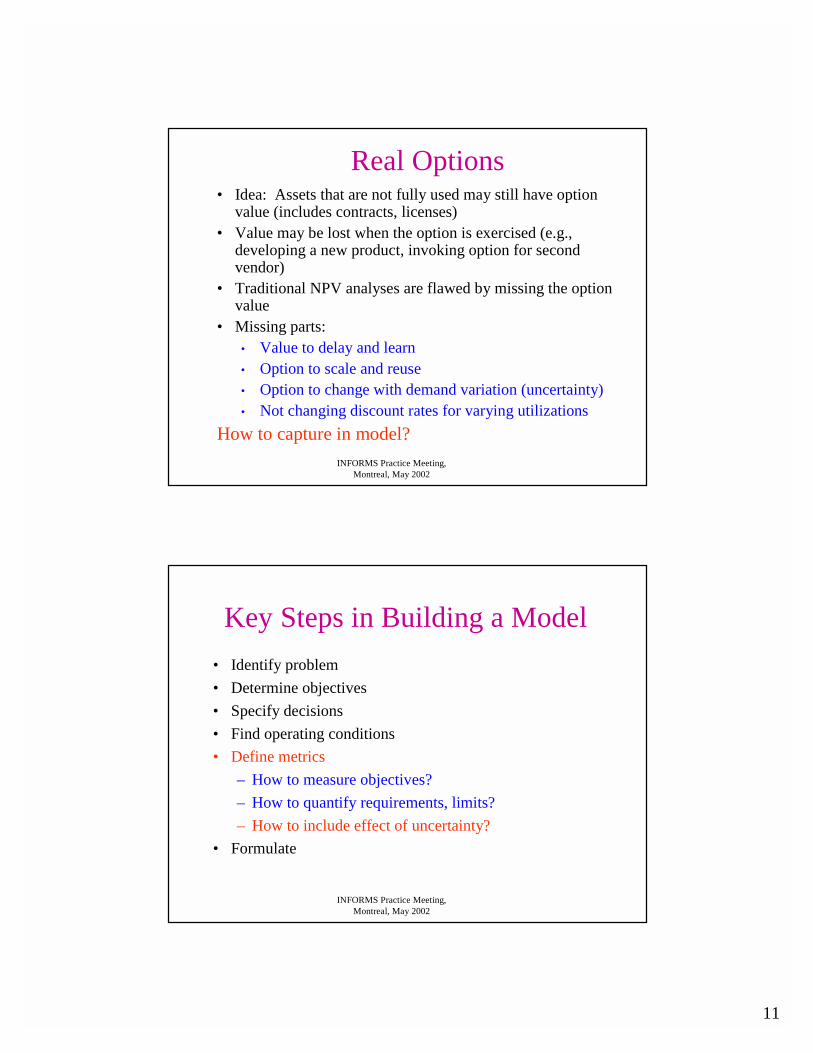
Real Options• Idea: Assets that are not fully used may still have option
value (includes contracts, licenses)• Value may be lost when the option is exercised (e.g.,
developing a new product, invoking option for second vendor)
• Traditional NPV analyses are flawed by missing the option value
• Missing parts:• Value to delay and learn• Option to scale and reuse• Option to change with demand variation (uncertainty)• Not changing discount rates for varying utilizations
How to capture in model?
INFORMS Practice Meeting, Montreal, May 2002
Key Steps in Building a Model• Identify problem• Determine objectives• Specify decisions• Find operating conditions• Define metrics
– How to measure objectives?– How to quantify requirements, limits?– How to include effect of uncertainty?
• Formulate
12
INFORMS Practice Meeting, Montreal, May 2002
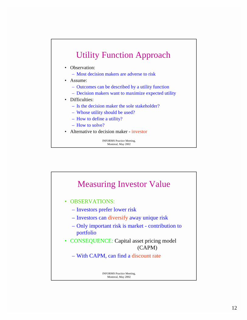
Utility Function Approach• Observation:
– Most decision makers are adverse to risk• Assume:
– Outcomes can be described by a utility function– Decision makers want to maximize expected utility
• Difficulties:– Is the decision maker the sole stakeholder?– Whose utility should be used?– How to define a utility?– How to solve?
• Alternative to decision maker - investor
INFORMS Practice Meeting, Montreal, May 2002
Measuring Investor Value
• OBSERVATIONS: – Investors prefer lower risk– Investors can diversify away unique risk– Only important risk is market - contribution to
portfolio• CONSEQUENCE: Capital asset pricing model
(CAPM)– With CAPM, can find a discount rate
13
INFORMS Practice Meeting, Montreal, May 2002
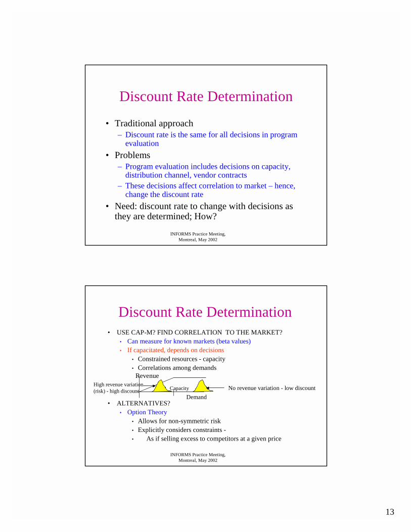
Discount Rate Determination
• Traditional approach– Discount rate is the same for all decisions in program
evaluation• Problems
– Program evaluation includes decisions on capacity, distribution channel, vendor contracts
– These decisions affect correlation to market – hence, change the discount rate
• Need: discount rate to change with decisions as they are determined; How?
INFORMS Practice Meeting, Montreal, May 2002
Discount Rate Determination• USE CAP-M? FIND CORRELATION TO THE MARKET?
• Can measure for known markets (beta values)• If capacitated, depends on decisions
• Constrained resources - capacity• Correlations among demands
• ALTERNATIVES?• Option Theory
• Allows for non-symmetric risk• Explicitly considers constraints -• As if selling excess to competitors at a given price
Revenue
DemandCapacity No revenue variation - low discountHigh revenue variation
(risk) - high discount
14
INFORMS Practice Meeting, Montreal, May 2002
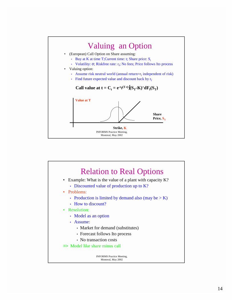
Valuing an Option• (European) Call Option on Share assuming:
• Buy at K at time T;Current time: t; Share price: St
• Volatility: σ; Riskfree rate: rf; No fees; Price follows Ito process• Valuing option:
• Assume risk neutral world (annual return=rf independent of risk)• Find future expected value and discount back by rf
Share Price, ST
Strike, K
Value at T
Call value at t = Ct = e-rf(T-t)∫∫∫∫(ST-K)+dFf(ST)
INFORMS Practice Meeting, Montreal, May 2002
Relation to Real Options• Example: What is the value of a plant with capacity K?
• Discounted value of production up to K?• Problems:
• Production is limited by demand also (may be > K)• How to discount?
• Resolution:• Model as an option• Assume:
• Market for demand (substitutes)• Forecast follows Ito process• No transaction costs
=> Model like share minus call
15
INFORMS Practice Meeting, Montreal, May 2002
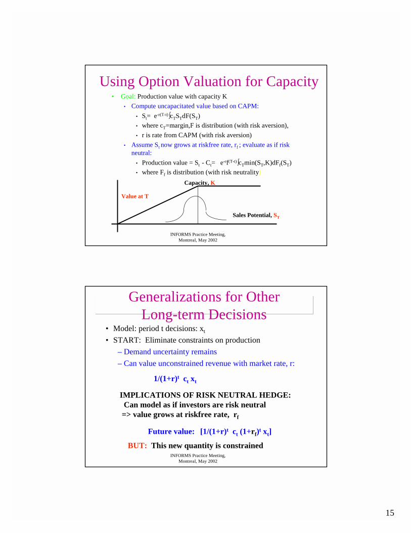
Using Option Valuation for Capacity• Goal: Production value with capacity K
• Compute uncapacitated value based on CAPM:• St= e-r(T-t)∫cTSTdF(ST)• where cT=margin,F is distribution (with risk aversion),• r is rate from CAPM (with risk aversion)
• Assume St now grows at riskfree rate, rf ; evaluate as if risk neutral:
• Production value = St - Ct= e-rf(T-t)∫cTmin(ST,K)dFf(ST)• where Ff is distribution (with risk neutrality)
Sales Potential, ST
Capacity, K
Value at T
INFORMS Practice Meeting, Montreal, May 2002
Generalizations for Other Long-term Decisions
• Model: period t decisions: xt
• START: Eliminate constraints on production– Demand uncertainty remains– Can value unconstrained revenue with market rate, r:
1/(1+r)t ct xt
IMPLICATIONS OF RISK NEUTRAL HEDGE:Can model as if investors are risk neutral
=> value grows at riskfree rate, rf
Future value: [1/(1+r)t ct (1+rf)t xt]
BUT: This new quantity is constrained

16
INFORMS Practice Meeting, Montreal, May 2002
New Period t Problem: Linear Constraints on Production
• WANT TO FIND (present value):MAX [ ct xt (1+rf)t/(1+r)t | At xt (1+rf)t/(1+r)t <= b]1/ (1+rf)t
EQUIVALENT TO:
MAX [ ct x | At x <= b (1+r)t/(1+rf)t]1/ (1+r)t
MEANING: To compensate for lower risk with constraints,constraints expand and risky discount is used
INFORMS Practice Meeting, Montreal, May 2002
Constraint Modification• FORMER CONSTRAINTS: At xt <= bt
• NOW: At xt (1+rf)t/(1+r)t <= bt
•xt
•bt
•xt(1+rf)t/(1+r)t
•bt
17
INFORMS Practice Meeting, Montreal, May 2002
EXTREME CASES
All slack constraints:1/ (1+r)t MAX [ ct x | At x <= b (1+r)t/(1+rf)t]
becomes equivalent to:
1/ (1+r)t MAX [ ct x | At x <= b]
i.e. same as if unconstrained - risky rate
NO SLACK:becomes equivalent to:
1/ (1+r)t [ct x= B-1b (1+r)t/(1+rf)t]=ct B-1b/(1+rf)t
i.e. same as if deterministic- riskfree rate
INFORMS Practice Meeting, Montreal, May 2002
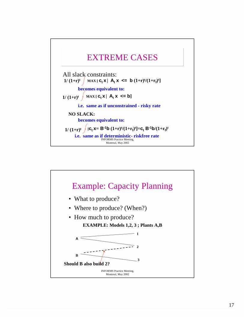
Example: Capacity Planning• What to produce?• Where to produce? (When?)• How much to produce?
A1
2
3B
EXAMPLE: Models 1,2, 3 ; Plants A,B
Should B also build 2?

18
INFORMS Practice Meeting, Montreal, May 2002
Result: Stochastic Linear Programming Model
• Key: Maximize the Added Value with Installed Capacity• Must choose best mix of models assigned to plants• Maximize Expected Value over s[Σi,t e-rtProfit (i) Production(i,t,s) -
CapCost(i at j,t)Capacity (i at j,t)]• subject to: MaxSales(i,t,s) >= Σ j Production(i at j,t,s)• Σ i Production(i at j,t,s) <= e(r-rf)t Capacity (i,t) • Production(i at j,t,s) <= e(r-rf)t Capacity (i at j,t)• Production(i at j,t,s) >= 0
• Need MaxSales(i,t,s) - random• Capacity(i at j,0) - Decision in First Stage (now)
NOTE: Linear model that incorporates risk
INFORMS Practice Meeting, Montreal, May 2002
Result with Option Approach
• Can include risk attitude in linear model• Simple adjustment for the uncertainty in
demand• Requirement 1: correlation of all demand to
market• Requirement 2: assumptions of market
completeness
19
INFORMS Practice Meeting, Montreal, May 2002
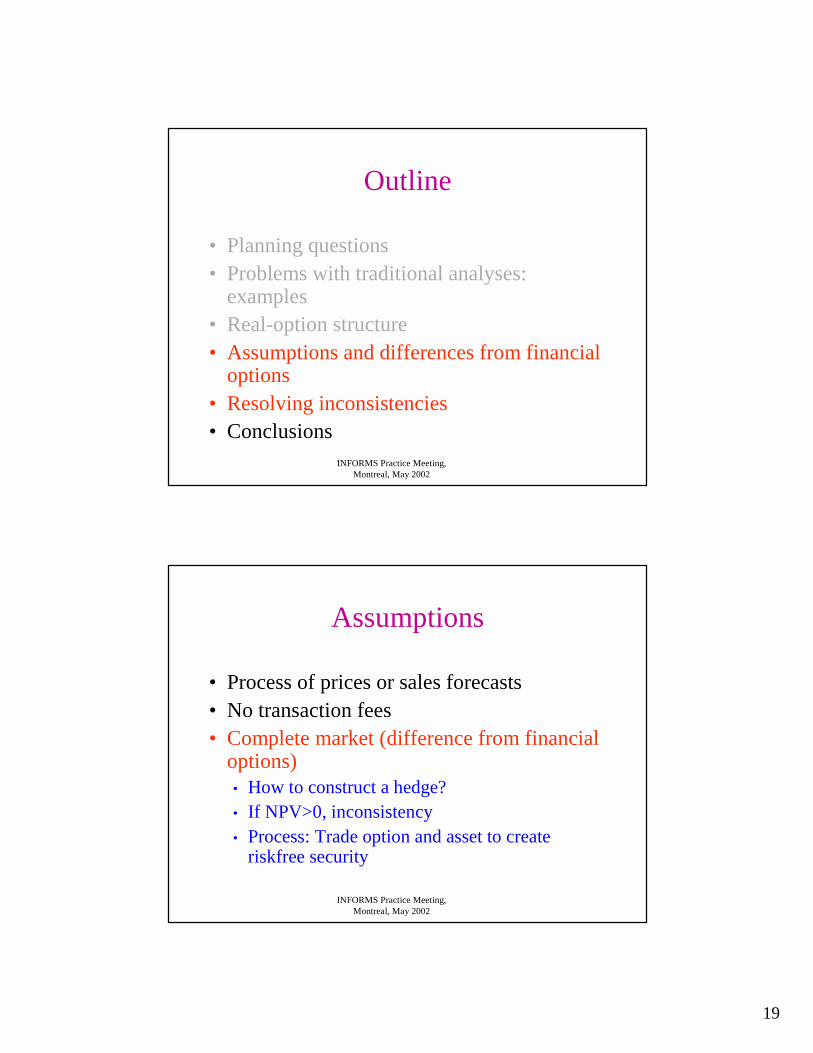
Outline
• Planning questions• Problems with traditional analyses:
examples• Real-option structure• Assumptions and differences from financial
options• Resolving inconsistencies• Conclusions
INFORMS Practice Meeting, Montreal, May 2002
Assumptions
• Process of prices or sales forecasts• No transaction fees• Complete market (difference from financial
options)• How to construct a hedge?• If NPV>0, inconsistency• Process: Trade option and asset to create
riskfree security
20
INFORMS Practice Meeting, Montreal, May 2002
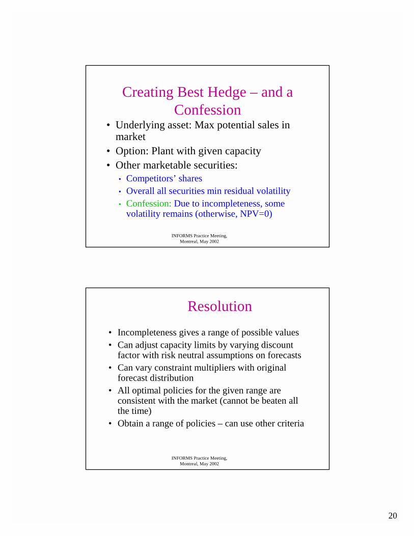
Creating Best Hedge – and a Confession
• Underlying asset: Max potential sales in market
• Option: Plant with given capacity• Other marketable securities:
• Competitors’ shares• Overall all securities min residual volatility• Confession: Due to incompleteness, some
volatility remains (otherwise, NPV=0)
INFORMS Practice Meeting, Montreal, May 2002
Resolution
• Incompleteness gives a range of possible values• Can adjust capacity limits by varying discount
factor with risk neutral assumptions on forecasts• Can vary constraint multipliers with original
forecast distribution• All optimal policies for the given range are
consistent with the market (cannot be beaten all the time)
• Obtain a range of policies – can use other criteria
21
INFORMS Practice Meeting, Montreal, May 2002
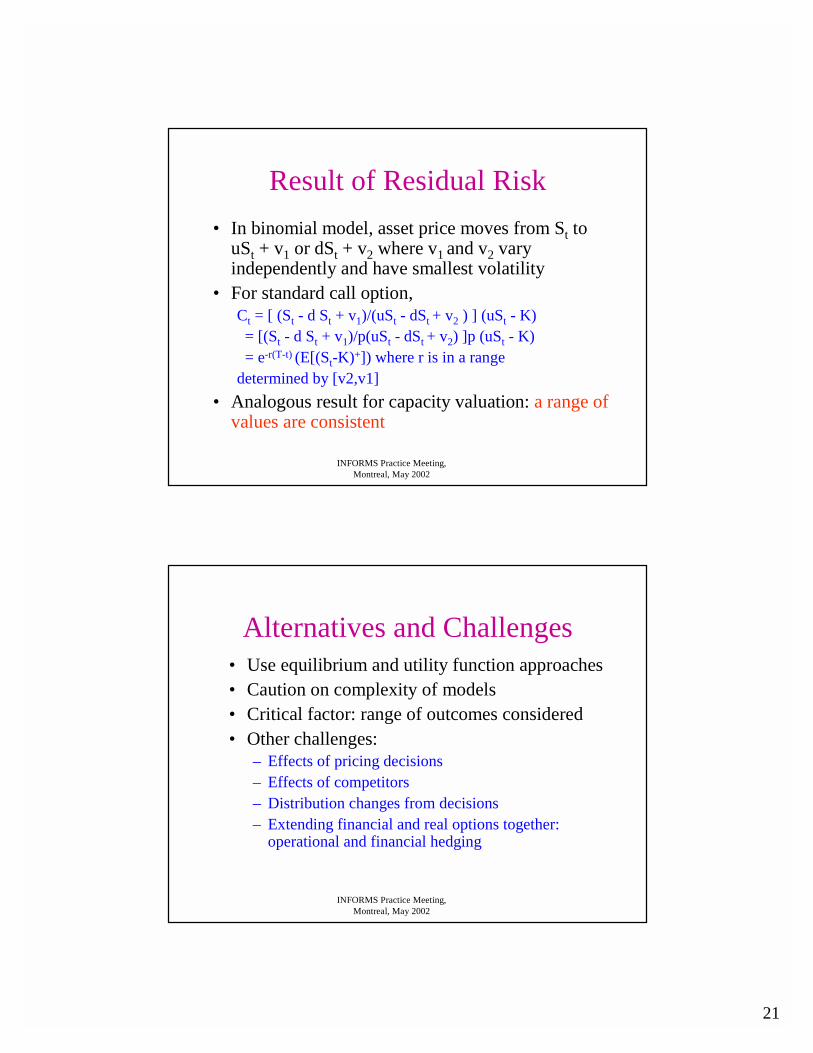
Result of Residual Risk• In binomial model, asset price moves from St to
uSt + v1 or dSt + v2 where v1 and v2 vary independently and have smallest volatility
• For standard call option, Ct = [ (St - d St + v1)/(uSt - dSt + v2 ) ] (uSt - K)
= [(St - d St + v1)/p(uSt - dSt + v2) ]p (uSt - K)= e-r(T-t) (E[(St-K)+]) where r is in a range
determined by [v2,v1]• Analogous result for capacity valuation: a range of
values are consistent
INFORMS Practice Meeting, Montreal, May 2002
Alternatives and Challenges• Use equilibrium and utility function approaches• Caution on complexity of models• Critical factor: range of outcomes considered• Other challenges:
– Effects of pricing decisions– Effects of competitors– Distribution changes from decisions– Extending financial and real options together:
operational and financial hedging
22
INFORMS Practice Meeting, Montreal, May 2002
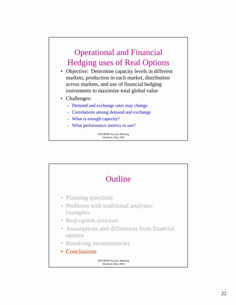
Operational and Financial Hedging uses of Real Options
• Objective: Determine capacity levels in different markets, production in each market, distribution across markets, and use of financial hedging instruments to maximize total global value
• Challenges:• Demand and exchange rates may change• Correlations among demand and exchange• What is enough capacity?• What performance metrics to use?
INFORMS Practice Meeting, Montreal, May 2002
Outline
• Planning questions• Problems with traditional analyses:
examples• Real-option structure• Assumptions and differences from financial
options• Resolving inconsistencies• Conclusions
23
INFORMS Practice Meeting, Montreal, May 2002
Summary
• Options apply to many varied decision problems• Can evaluate planning with proper option
evaluation techniques• Relaxed market assumptions lead to models that
determine a range of policies• Firm or investor utility can choose within range• Questions? Comments?