wage determination in russia: an econometric investigation · wage determination in russia: an...
TRANSCRIPT
Wage Determination in Russia: An EconometricInvestigation
By: Peter J. Luke and Mark E. Schaffer
Working Paper Number 295March 2000

Wage Determination in Russia:An Econometric Investigation
Peter J. [email protected]
andMark E. Schaffer
Centre for Economic Reform and TransformationDepartment of Economics
School of ManagementHeriot-Watt University
Edinburgh EH14 4AS, UK
March 2000
Abstract
Using a firm level dataset from four regions of Russia covering 1996/97, aninvestigation was carried out into how the surplus created within the firm is dividedbetween profits and wages. An efficient bargaining framework based on the work ofSvejnar (1986) is employed which takes into account the alternative wage or outsideoption available to employees in the firm as well as the value added per employee.Statistical differences in the share of the surplus taken by employees employed instate, private and mixed forms of firms are found. In addition, the results provesensitive to the presence of outliers and influential observations. A variety ofdiagnostic methods are employed to identify these influential observations and robustmethods are employed to lessen the influence of them. Whereas in practice some ofthe diagnostic and robust methods utilised proved incapable of identifying oraccommodating the gross outlier(s) in the data, the more successful methods includedrobust regression, Winsorising, the Hadi and Siminoff algorithm, Cook’s Distanceand Covratio.
JEL Classification: C21, J300.
Keywords: Russian labour markets, efficient bargaining, outliers, regressiondiagnostics, robust regression.
AcknowledgementsThe authors would like to thank Dr Hartmut Lehmann and Professor Joep Konings for helpfulcomments and discussion. Financial support from the European Union’s Tacis-Ace Research ProjectT-95-4099-R is gratefully acknowledged. We are also grateful to participants of the project closingworkshop for useful comments and suggestions. The usual caveat applies.

3
1. Introduction
This paper investigates wage determination in Russia. Wage equations derived from anefficient bargaining model are estimated econometrically on a new firm-level datasetfor 1996–97 covering several thousand industrial and construction firms from fourregions of Russia. The central economic question investigated in the paper is howwage determination is related to form of ownership. In particular, we ask whether thedegree of state ownership – full state ownership, fully privatised, or mixed state/privateownership – is related to the share of the firm’s surplus taken by workers. Do workersin state-owned firms take a larger share of the surplus than in private firms, as our exante expectation of the nature of corporate governance would suggest? Is wagedetermination in partially privatised firms more akin to that in state-owned or in privatefirms?
The ‘outside option’ or ‘alternative wage’ – the expected income faced by workerswho leave a firm – plays an important role in wage bargaining models of this type. Thepaper makes two contributions in this regard. First, we relax the usual modelingassumption that the alternative wage is exogenous, and derive from the model theimplications of what happens when the wage set by a (large) firm has an impact onwages set by other firms – a not unrealistic possibility for Russia, where labour marketsare highly segmented regionally, and wage setting by individual firms may have ageneral impact on wage setting in the region. Second, in our empirical work wecalculate and work with a firm-specific alternative wage that is intended to capturealternative employment possibilities within the same sector and region as the firm. Themotivation for this is again the regional segmentation of Russian labour markets.
Finally, our empirical investigation directly addresses a practical problem facing manyresearchers conducting econometric analyses using data from transition countries – theproblem of ‘dirty data’ or outliers. Rather than deal with this problem in an ad hocway, as most investigators do, we employ a wide range of econometric methods ofoutlier detection and robust estimation. We find that the econometric estimates of themodel can indeed be highly sensitive to the treatment of outliers. The general lessonfrom this is that when investigators suspect the data they are using are ‘dirty’, theyshould conduct and report a range of outlier detection and robust estimationtechniques.
The paper is organised as follows. Section 2 presents the theoretical and estimatingframeworks used in the paper. Section 3 discusses various econometric techniques foroutliers and robust estimation. The dataset used and the estimation results aredescribed in Sections 4 and 5, respectively. Section 6 concludes.
4
2. Theoretical and Estimating Frameworks
2.1. Right-to-Manage vs. Efficient Bargaining
In attempting to model how insiders may raise their wage above the outside option or‘alternative wage’ – the wage that can be expected to be earned by a worker werehe/she to leave his/ her current job – various approaches have been taken by differentresearchers.
The question boils down to whether the firm is on its labour demand curve or on thecontract curve. This is often expressed as the right-to-manage model versus theefficient bargaining model.1 In the former model, the two sides within the firm –management and workers – bargain over the wage but not employment, manangementthen sets the level of employment given the wage, and the outcome lies somewhere onthe labour demand curve. In the latter model, both parties bargain over wages andemployment and employment will be higher than if they bargain only over wages;efficient from the perspective of the firm but not of society as a whole.2
In its general form the right-to-manage model has a generalised Nash bargainingsolution which is the product of the weighted net gains to each party: the gain toemployees from expected income (from either employment in the firm or alternativeemployment) over certain alternative employment, and the gain to the firm from profitsearned vs. shut-down or zero profits.
( ) ( ){ }
( ){ } γγ
γγ
−
−
−
−=
−−
−−+=
1A
1AA
w
wLLpQ)]w(u)w(u[T
L
0wLLpQ)w(u]wu)T
L1()w(u
T
L[B max
(1)
where L is employment, w is the wage, wA is the alternative wage, u is utility fromwage income, Q is output, wLpQ − is firm profits, γ is the bargaining strength of the
employees, and T can be interpreted as the number of all workers (in the Westerncontext, this would be union membership) including both those who end up beingemployed by the firm and those who are not employed by the firm and take alternative
employment instead. The weights L/T and ( TL1 − ) can be interpreted as the
probabilities faced by a representative worker of employment in the firm, and of havingto take alternative employment (including possibly being unemployed), respectively.Bargaining (maximisation) is over the wage w, and the employment level L is chosenby the firm to maximise profits. The efficient bargaining model has an identical setup,with the simple difference that bargaining (maximisation) is over both the wage w andthe employment level L, i.e.,
1 See, in particular, for a very good summary of the issues, Booth (1995).2 See, however, Layard and Nickell (1990) who show that this is only true under limited assumptions.
5
( ) ( ){ } γγ
−−
−= 1
AL,w
wLLpQ]wu)w(u[T
LB max (2)
Which of the two models would be more appropriate for modeling wage andemployment determination in the Russian transition economy is a difficult question, asthere is little micro empirical evidence on whether or how far bargaining withinRussian firms extends beyond wage bargaining to include bargaining over employment.The labour hoarding that still continues today within Russian enterprises can beinterpreted either within an efficient bargaining model, or, in a right-to-manageframework in which wages are extremely flexible, where employees have simply tradedoff real wages for relative employment security and in the process moved (a long way)down the labour demand curve.3
In practice, however, the two models yield very similar estimating equations. As Boothpoints out,4 there is as yet no clear test to discriminate between the two models. Forour purposes, the choice of model is mostly one of convenience. We use in this paperan efficient bargaining model by Svejnar (1986) that has also been used to estimatewage equations in a transition context (Prasnikar et al., 1994 and 1997).
2.2. Estimating Framework
Svejnar (1986) sets out a Nash bargaining model of wage determination in whichunions have fixed memberships and maximise their members’ expected utility which istaken as a function of income and employment; the firm’s utility is taken as equal totheir profit. In the context of a transition economy such as the Russian Federation it isnot labour unions but firm insiders that are seeking to maximise utility.
In Svejnar’s model, Y is total labour income and the union utility function V reflectsconstant relative risk aversion:
( )δ
δγ=YV (3)
and the coefficient of relative risk aversion is given by:
( )( )YV
YYVr
′′′−
= (4)
Note δ < 1 (δ > 1) implies risk aversion (risk loving). Svejnar’s final estimating model,
conditional on δ = 1, i.e., risk neutrality, is:
3 See, e.g., Standing (1996) who argues that wages in Russia have been extremely flexible and themain reason for low observed rates of unemployment.4 Op. cit. p. 135.
6
( )aY
L
HLaYRY +
−−= γ (5)
or
)valad(aYY γ+= (6)
where Y is the firm wage, Ya is the alternative wage or outside option, R is firm
revenue, H is non-labour costs, L is employment,5 L/)HLYR(valad a −−= is the
value added per worker evaluated at Ya, and γ as before is a measure of workers’
bargaining power. Value added per worker, valad, can be interpreted as the surplusper worker generated by the firm above the amount workers would obtain if they tookup their outside option. Note that the main implication of the above equation is that themeasure of insider power, γ will also be the share of value added that workers take
over and above the outside option. A value of one indicates that all added value istaken by the workers and so insiders have complete power. A value of zero indicatesthat the insiders have no power and receive only the outside option as a wage.
We are particularly interested in the impact of ownership form on wage formation, andtherefore in the estimations we allow both for ownership-specific coefficients on valadand ownership intercept dummies. The data allow us to distinguish between state-owned firms, privatised firms, and ‘mixed’ firms with both state and private ownershipshares. Our prior expectations are that the share of value-added appropriated byinsiders will be larger in state-owned firms than in private firms because of the superiorcorporate governance in the latter, with mixed firms being an intermediate case.
Currie (1991) in her study of teachers’ wages in Ontario uses an efficient contractsmodel and a standard labour demand model. The alternative wage is assumed to be alog-linear function of wages in surrounding school districts, average income in thedistrict, local manufacturing wages, and a local employment index. Ashenfelter andBrown (1986) in their particular study of union branches belonging to the InternationalTypographical Union actually use eleven different measures of the alternative wage.MaCurdy and Pencavel (1986) again using data on branches of the InternationalTypographical Union use a wage index representing the real hourly earnings receivedby production workers in durable goods manufacturing. The point to note from this isthat there does not appear to be a universal method of calculating the definitivealternative wage. It is very much a case of the particular circumstances determining theapproach to be taken.
5 Under the assumption of risk neutrality, i.e., δ = 1, Svejnar’s model leads to a vertical contract curveand hence a unique value of employment which coincides with the socially efficient level ofemployment, just as if the firm were on its labour demand curve paying its workers the outside optionor the alternative wage. This is a strong assumption especially given the situation within Russia.Svejnar later swaps this assumption for one of a Cobb-Douglas production function which allows thevalue of δ to vary.

7
If we wish to take into consideration unemployment and unemployment benefits then afurther complication arises. In the unemployment benefit system in the RussianFederation that has been in place since the early 1990s, there is no single measure ofunemployment benefit. Benefit is calculated as a percentage of the worker’s averagepay over the final three months of employment. At the time of writing the workerreceives 0.75 of this figure for a total of three months; a further 0.6 of their previousaverage pay for a maximum of four months after the first three months have expiredand a final 0.45 for a remaining five months with the possibility of a further six monthson top of this after a review. This is further complicated by the fact that there is aminimum and a maximum which the claimant can receive. If in the first three monthstheir calculated benefit exceeds the maximum then it is this maximum figure that theyreceive and not the 0.75 of their previous average wage. The final complication is thatthis maximum and minimum varies from oblast to oblast since it is calculated on amonthly basis using a basket of local consumer goods and hence local prices asopposed to the average price level for the country as a whole.
The Russian labour market is highly segmented, with very little labour mobilitybetween regions. Labour skills are also sector-specific. This implies that the alternativewage faced by a worker in a firm will be the wage in alternative employment in asimilar firm in the same region of Russia. Our strategy is to estimate the wage equationin which the alternative wage is calculated for each firm as the average wage in allother firms in the same sector and region; in other words, we make the alternativewage firm-specific:
∑
∑
≠
≠=n
ij,jj
n
ij,jj
i,a
firmemployment
firmfund wage
Y (7)
where n is the number of firms in a particular sector in a particular region.
We also recognise that recorded unemployment rates are likely to understate thedifficulty a departing worker will have in finding a new job; although observedunemployment rates in Russia are low, outflow rates from unemployment are also low.We therefore do not use observed unemployment rates to weight the alternative wagebut instead the coefficient on the alternative wage to vary from unity. Our priorexpectation here is that the coefficient will be positive but significantly less than one.
Our estimating equation is therefore:
i,aYivaladmixed
ivaladprivateivaladmixedprivateiY
βγ
γγααα
++
++++=(8)
8
where i is used to index observations on individual firms and the coefficients denoted‘private’ and ‘mixed’ are intercept and slope coefficients relating to the relevantownership dummy variables. We also include regional and industry dummy variables inthe estimation.
2.3. The Alternative Wage - Exogenous or Endogenous
Finally, there is a question mark on the endogeneity of the alternative wage. Lockwoodand Manning (1989) have shown that in a dynamic framework all variables that affectfirm profits will influence employment determination. However, for the purposes of theregressions, we have assumed, as Svejnar himself does, that the alternative wage isexogenous. This issue is, however, taken up when we allow the firm wage to vary withthe alternative wage.
In Svejnar (1986), as in the literature generally, the alternative wage is taken asexogenous and the change in the firm’s own wage is not seen to have any influence onthe alternative wage. However, it can be argued that if the individual firm is largeenough relative to the size of the branch in which it is operating, then any change in thefirm wage will be noticed by workers in other firms who will recalculate theiralternative wage on the basis of the new wage that they now see in effect in the other(large) firm. A change in the alternative wage for these workers will, as shown byMcDonald and Solow (1981), lead to a leftward movement of their contract curve andso to a higher wage. The workers who originally began the process see that theiralternative wage has increased and so their contract curve will move to the left and ahigher wage will result.
The above mirrors, to a degree, the annual wage round within Britain in the sixties andseventies in particular when individual unions were keen ‘to maintain differentials’ andmaintain their position within a pay league relative to other groups of workers. Wehave reworked Svejnar’s basic model for his estimating equation but allow Ya, thealternative wage, to be a function of Y, the firm wage.
( ) [ ] γγ
γγ −−−
−
=− 1HLiYRL
aYiYL1MULU (9)
In a two-party framework the bargaining process is the maximisation of the aboveequation. This leads to the following steps:
( ) =• iY / ∂∂
( ) [ ]
( ) ( )[ ] ( ) 0LHLiYR1L
aYiYL
L
LA
L
L1HLiYR1
LaYiYL
=−−−−−
−
+
−−−−
−
−
γγγ
γγ
γ(10)

9
where A equals ia YY ∂∂ . In the Svejnar model this conjectural variation has a value of
zero. Now we allow it to vary. One would expect a priori that it would take a valuebetween zero and one. If groups of workers are primarily concerned with keeping theirrelative positions in some kind of pay league then a value of one would implyunchanged positions in any ranking and a value of less than one would imply that the‘distance’ between groups of workers is widening. It can be shown that allowing thealternative wage to be endogenous results in the following formulation (seeAppendix 1).
( )aY
A1
A1
L
LaYHRiY +
−−
∗−−
=γ
γ (11)
This should be compared with equation (5) from the original model:
( )aY
L
LaYHRiY +
−−=
γ(5)
Thus if the wage set by a firm has an impact on the alternative wage, i.e., on the wagesset by other firms, the effect is to decrease the share of the surplus taken by the insidersof the firm, and the estimated coefficient on value added per worker will decrease.
3. Econometric Techniques for Outliers and Dirty Data
‘An outlying observation, or ‘outlier’, is one that appears to deviatemarkedly from other members of the sample in which it occurs.’6
‘Outliers occur very frequently in real data, and ... may totally spoil a least7
As is well known, there is a general problem with the reliability of data reportingwithin Russia. This arises for two reasons. Firstly, there is a problem related to therecording of the data by the relevant state statistical bodies.8 Outliers arising from thisfall within the realm of what are described as ‘non-statistical factors’.
The second problem is potentially more serious and arises from contamination fromanother distribution other than the one under consideration. Here we are concernedwith statistical factors that might help us explain why outliers occur, how they can be
6 Grubbs (1969) quoted by Barnett and Lewis (1994).7 Rousseeuw and Leeroy (1987).8 To give but a few examples from the data we use in this paper. Two firms apparently paid negativewages to their workforces. Another two recorded negative fixed capital. A file containing observationson trade related firms within the Moscow area had several hundreds of duplicate observationsmasquerading as unique observations. In the original data that were obtained, the area or regionalGoskomstat offices were using different units of account to measure the financial totals of somevariables; for example, the fixed capital figures from the Chuvash file had to be divided by 1000 toensure the same units were used throughout.

10
detected and if necessary whether they should be removed. For example, we may wishto examine the distribution of sales of Russian enterprises. If 60 per cent of enterprisesreport truthfully, but 40 per cent do not, then in effect we have two distributionsmasquerading as one.
Even if we assume there is no contamination, extreme values may well occur whichhave been truthfully reported and recorded by the relevant statistical body. Shouldthese values be deleted, ignored or somehow accommodated? As Thomas (1997)writes, ‘... most econometricians prefer to retain unusual observations in theirdatasets’. But he continues, ‘However, because OLS is so sensitive to suchobservations, other methods of observation are sometimes employed’. Reiss (1990)comments, ‘When an observation is both an outlier and influential, investigators usuallyreport regression results both with and without the observation’. Using a variety ofeconometric techniques that take on board the presence of outliers within the data, wepresent results based on the model outlined above. We focus in particular on theestimated relationship between ownership structure and the distribution of surplus(value added) and how it is affected by the removal of outliers; in other words, howrobust are the findings?
There are two types of outliers. One is where the residual formed from the difference
between the fitted iY and the actual iY shows up as particularly large. The second is
where the iX is far from the mass of iX ’s. This means, for example, that an outlier
will cause the direction of the fitted line to change but this will not show up in a highresidual. This is a leverage point and the observation is usually referred to asinfluential. While outliers and influential observations are conceptually different it isnot unusual to see influential observations simply referred to as outliers.
Identifying outliers when there is only one contained within a dataset is relativelystraightforward. If there is more than one then problems can arise from what is knownas masking and swamping effects. Masking occurs when a subset of outliers is notdetected because of the presence of another subset, usually close to the former.Swamping, on the other hand, occurs when ‘normal’ observations are taken as outliersby the detection process because of the presence of another subset of observations.
One approach to outlier identification is to make use of the residuals from the modelestimation. However, given the normal error model the difficulty arises that theestimated residuals do not have constant variance (Behnken and Draper, 1972). Thevariance of the OLS residuals is given by:
( ) ( )
−−−
−= ∑
n
1
2i
2i2i xxxx
n
11)var( σε (12)
As can be seen the ith individual residual is not homoskedastic and is more variable the
closer the ix explanatory variable is to the overall mean. This ‘ballooning’ effect, as it
11
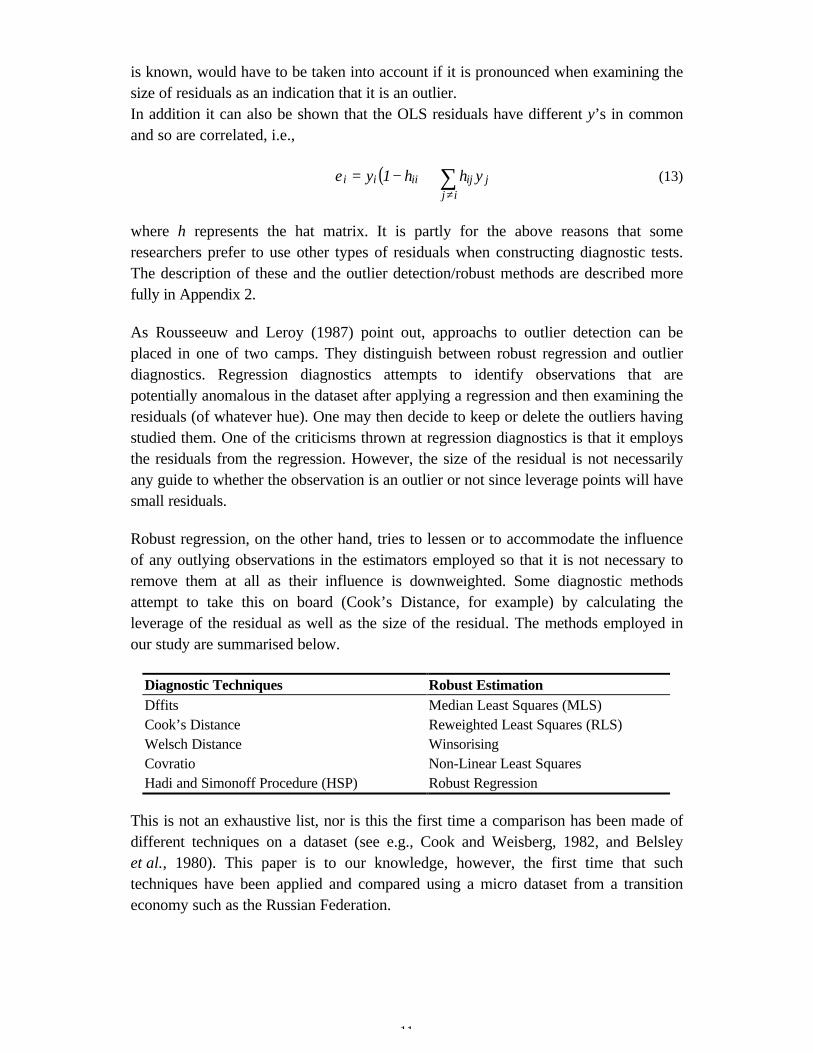
is known, would have to be taken into account if it is pronounced when examining thesize of residuals as an indication that it is an outlier.In addition it can also be shown that the OLS residuals have different y’s in commonand so are correlated, i.e.,
( ) ∑≠
+−=ij
jijiiii yhh1yε (13)
where h represents the hat matrix. It is partly for the above reasons that someresearchers prefer to use other types of residuals when constructing diagnostic tests.The description of these and the outlier detection/robust methods are described morefully in Appendix 2.
As Rousseeuw and Leroy (1987) point out, approachs to outlier detection can beplaced in one of two camps. They distinguish between robust regression and outlierdiagnostics. Regression diagnostics attempts to identify observations that arepotentially anomalous in the dataset after applying a regression and then examining theresiduals (of whatever hue). One may then decide to keep or delete the outliers havingstudied them. One of the criticisms thrown at regression diagnostics is that it employsthe residuals from the regression. However, the size of the residual is not necessarilyany guide to whether the observation is an outlier or not since leverage points will havesmall residuals.
Robust regression, on the other hand, tries to lessen or to accommodate the influenceof any outlying observations in the estimators employed so that it is not necessary toremove them at all as their influence is downweighted. Some diagnostic methodsattempt to take this on board (Cook’s Distance, for example) by calculating theleverage of the residual as well as the size of the residual. The methods employed inour study are summarised below.
Diagnostic Techniques Robust EstimationDffits Median Least Squares (MLS)Cook’s Distance Reweighted Least Squares (RLS)Welsch Distance WinsorisingCovratio Non-Linear Least SquaresHadi and Simonoff Procedure (HSP) Robust Regression
This is not an exhaustive list, nor is this the first time a comparison has been made ofdifferent techniques on a dataset (see e.g., Cook and Weisberg, 1982, and Belsleyet al., 1980). This paper is to our knowledge, however, the first time that suchtechniques have been applied and compared using a micro dataset from a transitioneconomy such as the Russian Federation.
12
4. The Dataset and Summary Statistics
The data cover a three year period from 1995 to 1997 and come from Goskomstat, theRussian Federation state statistical body. The information is collected from all medium-sized and large firms, of all categories of ownership – state-owned, privatised, and‘mixed’ firms with both private and state ownership shares. The four regions coveredare Moscow City, Krasnoyarsk Krai, Chuvashia Republic and Chelyabinsk Oblast.9 Thedata cover all medium and large industrial and construction firms in these regions.10
As argued above, it is appropriate in the Russian case to treat the alternative wage asregion- and sector-specific. Alternative wages at the two-digit branch level werecalculated as follows.11 First, the ‘branch wage fund’ and ‘branch employment’ werecalculated for each of the four regions in the data. Second, for each firm, that firm’swage fund and employment level were subtracted from the branch wage fund andbranch employment, respectively, to generate an alternative branch wage fund and analternative employment level (given the same branch and location). Finally, the formerdivided by the latter gives the alternative wage for each firm. The alternative wage thuscalculated can be interpreted as the wage a worker would expect, on average, ifleaving his current job and taking a job in a different firm in the same branch in thesame region.
The wage fund is made up of monetary payments for labour activities performed andof payments in kind. The fund takes in incentive payments, bonuses and specialpayments connected with the conditions of work (dangerous or harmful conditions,night working, overtime payments etc.). Also included in the wage fund are regularpayments on food, fuel and living accommodation that are received by the workforceeither as a result of agreements between the workforce and management or due tolegislation. Paid holidays, leave for training and professional retraining are alsoincluded in this. The average wage for each firm was calculated as the firm wage funddivided by the average listed number of workers.
Value added per worker is calculated as the sum of the wage fund and reported profits,less the alternative wage (see above). Profit is calculated according to the standardRussian definition except that it is gross of depreciation. Depreciation is not reporteddirectly in the data but is instead estimated for each firm using reported fixed capitaland the average depreciation rate for Russian industries reported in the annualstatistical yearbook published by Goskomstat.
9 The reasons for choosing them as representative economic regions within the Russian Federation arediscussed in Lehmann, Wadsworth and Acquisti (1998).10 The raw data also cover wholesale and retail trade firms, but missing data meant there was aninsufficient number of firms from these sectors to be included in the study.11 The two-digit levels means, for example, the fuel sector (11), ferrous and non-ferrous metals (12),machine construction (14) and so on.
13
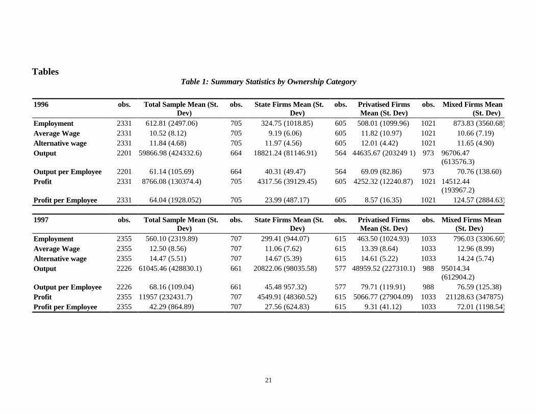
Tables 1–2 present summary statistics for the data that relate to those observationsactually used in the regression analysis, i.e., excluding firms with incomplete data.Output and output per worker, while not used in the estimating equation, are alsopresented.12 All financial data are current prices in millions of rubles.
5. Estimation Results
Table 3 below gives the results obtained from using the above methods on the datasetwhen applied to the basic model estimated in levels for the year 1997. The first columnreports the results of estimating the model on the full sample of data using ordinaryleast squares (OLS). Subsequent columns report estimation after deletion of outliersand/or using the named robust estimation technique. The number of observationsdropped as outliers in each estimation is reported in the last row of the table. Theomitted regional intercept dummy variable is Chelyabinsk.
Starting first with outlier detection methods, several results are worth stressing. Ingeneral the largest reduction in the residual sum of squares caused by the removal of asubset of n observations from a dataset are seen as the most likely candidates to beoutliers (Gentleman and Wilk, 1975). Put another way the greatest increase in the R2 isone way to discriminate between different outlier detection methods. On that basis, theHadi and Simonoff procedure (HSP) performs best – the R2 increases from 0.29 withthe full sample to 0.66 when the outliers are deleted. Cook’s distance and covratio arenext with R2 ’s of 0.47 and 0.48, respectively. Welsch’s distance and Dffits, however,actually decrease the R2 by the deletion of their outliers.
Turning to the robust estimation techniques two methods stand out – winsorising androbust regression. In the latter case, an R2 is not applicable because of the weightingprocedure. The coefficents generated by robust regression are close to Cook’sdistance, which follows from the fact that this robust regression technique uses Cook’sdistance initially to remove ‘gross outliers’ (see Appendix 2). The R2 from thewinsorised regression is of the same magnitude as the HSP and the coefficientsproduced between the two methods are, relatively speaking, very similar.
In the course of the study it was found that there was one very influential observation.Its deletion results in a dramatic change in the coefficients and in the value R2 – see thefinal column in Table 3, ‘Minus One’. The coefficient on value added per employee, forexample, jumps from 0.001 to 0.27; on the interactive dummies for value added peremployee they change from 0.071 and –0.001 to –0.198 and –0.270 for private andmixed property firms, respectively.
Further examination of the results reported in Table 3 show that the estimation resultscan be separated into two groups: those in which the estimated coefficient on value
12 A small number of firms do not report output data but report profit, wage and employment data andhence can be included in the regression analysis.
14
added per worker is extremely small, about 0.001 – OLS applied to the full sample,Dffits, Welsch’s distance, non-linear least squares, and median least squares – andthose in which the estimated coefficient is between 0.27 and 0.33, values that arerelatively reasonable and consistent with our prior expectations – HSP, Cook’sdistance, Covratio, robust regression, Winsorising, and ‘Minus One’. What ishappening is that the HSP, Cook’s distance, covratio, robust regression andWinsorising methods pick up this gross outlier while the other methods do not.
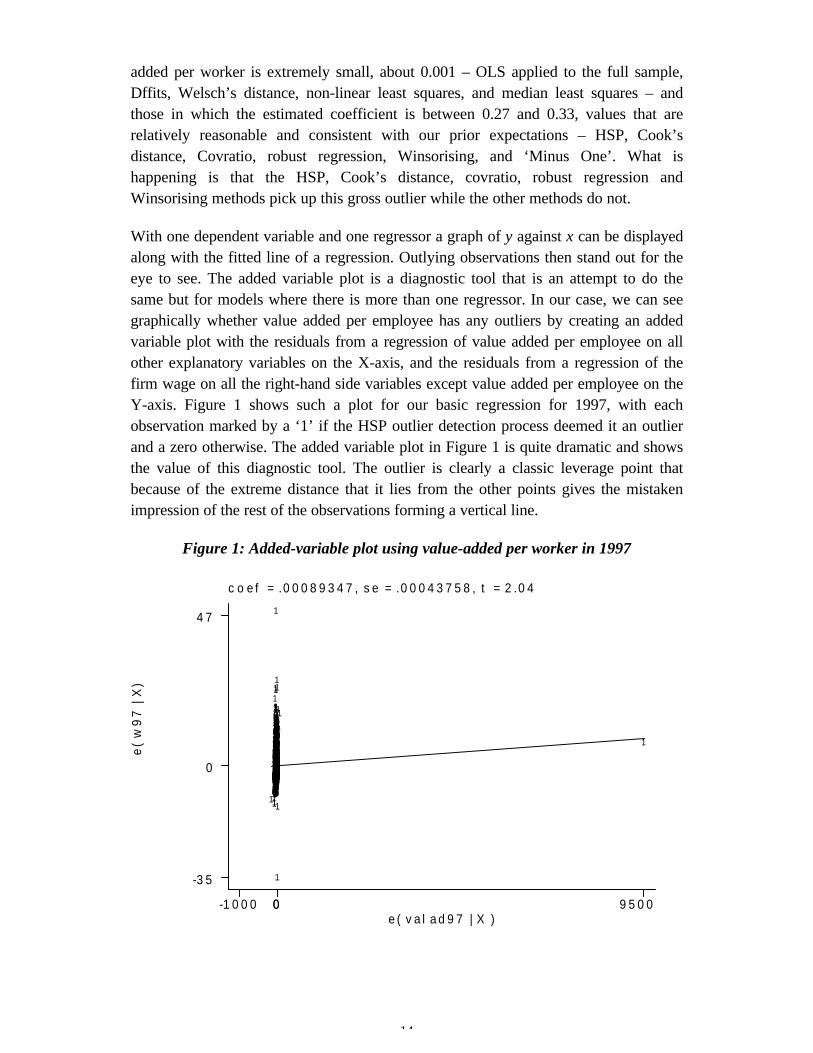
With one dependent variable and one regressor a graph of y against x can be displayedalong with the fitted line of a regression. Outlying observations then stand out for theeye to see. The added variable plot is a diagnostic tool that is an attempt to do thesame but for models where there is more than one regressor. In our case, we can seegraphically whether value added per employee has any outliers by creating an addedvariable plot with the residuals from a regression of value added per employee on allother explanatory variables on the X-axis, and the residuals from a regression of thefirm wage on all the right-hand side variables except value added per employee on theY-axis. Figure 1 shows such a plot for our basic regression for 1997, with eachobservation marked by a ‘1’ if the HSP outlier detection process deemed it an outlierand a zero otherwise. The added variable plot in Figure 1 is quite dramatic and showsthe value of this diagnostic tool. The outlier is clearly a classic leverage point thatbecause of the extreme distance that it lies from the other points gives the mistakenimpression of the rest of the observations forming a vertical line.
Figure 1: Added-variable plot using value-added per worker in 1997
coef = .00089347, se = .00043758, t = 2.04
e( w
97 |
X)
e( valad97 | X )-1000 00 9500
-35
0
47
1
00010
1110
11
1
11
1
1
11
1
011
001
1
0
000
00
1
000
000
0
00000
0
0
0
0
0
00000
00
000
0
0
0
00000
0
0
0
00
00
0
1
0
0
0
000
0
1
010
0
0
1
00
1
0
0000
0
00
1
000
000000
0
0
0
000
00000
0
00000000000
000
0
0
00000000
00000
01000
000000000000
0
0000
0
0
0
01
00
0
000000
0
000000000
0000000000
0
0
00
0000
00000
000000
00000
00
0000000
0
0
0
0
0
000
0
000
1
0
0
00000
0
0
0
0
0
1
00
000000000000000000000
0
0
0
00
0
0
0
0
0
0
0000
0
00
0
0
0000000
0
000
0
0
00
0000
0
001
0
0
0
00000000000000
1
00
0
1
0000
1
0000
00000
0
000000000000
00
00000000000000000000000000000000000
000
0
00
000000000000
0
000000
1
0000
0
00
0
00000
1
0
000000000000
0
00000
0000000000000
0
000
0000000000000000000
00
00000
0
0000000
0
00
0
000
0
0
00
0
00
0
1
0
0100
1
00000000000
0
000
0000000
1
0000
0
0000000000000000000
00000000
0
0
00000
0
00000000000000000000000000000
0
00000
0
1
00
00
00
0
00000
0000000
1
000000000000
1
0000000000000000000000000000000000
0
000
0
00
00
0
00
0
0000000
0000
000000000
000
0
00
00000000000000000
0000
0
000000
000000
0
000
0
0
0
000000
0
0
0
00000
0
0
0
0
0
0
00
00
0
0
0
00
00100
1
1
1
0000
00
1
0000000000
1
00
0000
1
0000000000000000000000
0000000000000
0
0
0000000
0
00000000000
0000
00000000000000000000
0
0000000
0
000000000000000
0
000
000000
0000
000000
0000
0
0
000000000
0
0
00000000000
0
0000000000000000
0
000
0
000
000000000
000000000000000
0
0000000000000
0
0000000000
0000000000000
00
1
00
00
0
0
0000000000000000000
0
000
00000000000000000000
0000
00
00
000000
0
00000000000
000000000000000
0000
000
000000
0
00
0
0000000110
0
0000
000
0
0000000
000000
000
00000000000000000
0
000
0
0
0000000000000
0
00
0
000
0
000000
0
1000000
0
001
000
00
000
0
00
00000
00
000
0
000000000000000000000000
000000010000
000
000
000
10
0
0
000
00
000
0000000000000000
000
0
00000101100
1101
0
100
000
0
0000000000
0
0
000000
0
000000
00
000000000000000
00000000000
0
000000
000000
00000
0
0000000
000
0
0000
00
0
0000000000000
000
0
0
0
0001000100
0
1
00
00
0
0000000000
010
000000000000000
000
00
0000
00
000000000000
0
00000000000000000000
0
0
0000000000
0000
000000
0000000000
1
0
00
10
00
0
0
0
000000000000000000000000000000000000000000
0000
0000
000000000000000000000000000
0000
0
000
0
00000
0
00010
000000000
0
0
00
0
0
000
1
00000000010
0
00000000000000001
0100
1
00000010000000000000
0
0
0000000000000
000
0
0
0
0000
0
000000000000000000
0
1
0
0
0
0
00
00
0000000
0
000
0000
0
010
000000
0
0000000000000000000000000000000000
0
000000
0001
000000000000000000
000000000
0000
000000000
00000
0000000000000000000000000000000000
0000000000000000000000000
000
000000000
0
0000000000
0
00
000
000
0
000
00
00
00
000
0
1
0
1
0
000
0000
0
00000000
000000
0
0
0
0
0
0
0
0
00100000000000
0
0
0
0
0
101
000
1
000
00000000
1
00000000000000000000000000
00000000
000000000000000000
0000000000000000000
0000000000000000000000000
00000000000000000
0
0
0
00000010
000
10
100000
0
00
000
1
00
0000000
0
0
0
0
01
1
0
01
0
1
1
11
1

15
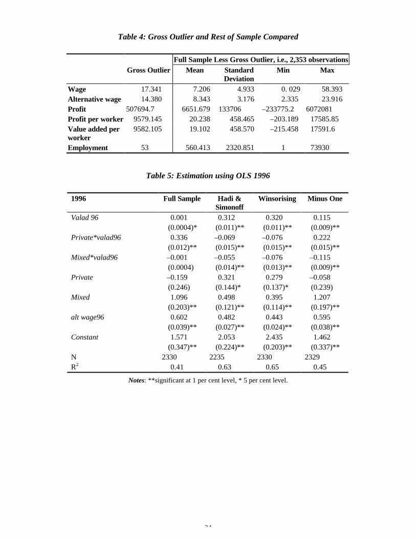
This gross outlier provides an acid test for the regression diagnostics employed alongwith the robust estimating techniques. The observation is contained within theKrasnoyarsk region, is a state-owned firm and is in the construction sector. Statisticalinformation on it and the rest of the data are presented separately in Table 4. It can beseen that this firm has an extremely high value of profits per worker, withunremarkable values for the other variables. We note that this outlier is not the resultof a simple reporting error – the same firm reports a very large value for profit in thepreceding year, 1996, as well.
Our first conclusion, therefore, is that even sophisticated outlier detection methods androbust estimation techniques can fail to detect a gross outlier whose presence in thedataset can have an overwhelming influence on the regression results.
Compared to the coefficients on value added per employee the coefficients on thealternative wage are relatively stable regardless of which technique is employed. Thevalue of the coefficient varies from 0.538 to 0.720. This is significantly less than unity,and is consistent with our prior expectations (see above).
We turn now to the estimated coefficients on value added per worker for the differentownership categories, considering only the results from the six methods that excludedthe gross outlier: HSP, Cook’s distance, Covratio, robust regression, Winsorising, andsimple exclusion of the gross outlier (‘Minus One’). The benchmark ownershipcategory is state-owned firms; the interactive coefficients on valad97 reported forprivate and mixed firms are deviations from this benchmark category. The value of theshare of the surplus taken by insiders for these ownership categories is obtained fromthe sum of the benchmark (state) coefficient and the estimated coefficient. Forexample, the coefficient on valad97 in the HSP results is 0.339, indicating that workersin state-owned firms appropriate 33.9 per cent of the available surplus. The coefficienton private*valad97 is –0.045, indicating that workers in private firms appropriated –4.5 per cent less than workers in state-owned firms, or 29.4 (33.9 – 4.5) per cent ofthe available surplus.
All six methods show that the share of the surplus taken by workers in private firms issignificantly less than that taken by workers in state-owned firms; the range of theestimated difference is from 4.2 percentage points less (Covratio) to 19.8 percentagepoints less (‘Minus One’). Note that the value of the coefficient for ‘Minus One’ issignificantly larger that those for the other methods, suggesting that the other methodsare detecting and excluding other, less gross, outliers.
The results for mixed ownership firms are themselves rather mixed. The estimations forthe HSP and winsorising show that the shares of surplus taken by workers in mixedownership firms are close to the shares taken by those in private firms, whereas theresults for Cook’s distance, covratio, robust regression, and ‘Minus One’ indicate thatworkers in mixed ownership firms are appropriating much smaller shares of the surplusthan in either state-owned or private firms. Indeed, the coefficient on mixed*valad97

16
in these latter results is approximately the same magnitude as, but opposite in signfrom the coefficient on valad97 – indicating, in other words, that workers in mixedfirms have zero bargaining strength and are appropriating none of the firms’ surplus.The former set of results – bargaining power in mixed firms similar to that of privatefirms – is more or less consistent with our prior expectations, the interpretation beingthat private ownership leads to lower bargaining power for workers regardless ofwhether it is full or partial private ownership. The latter set of results – workers inmixed firms have no bargaining power at all – is, however, harder to explain. Onepossibility, of course, is that the latter results are generated by outliers remaining in thesample but that are removed or attenuated by the HSP or Winsorising procedures; thisis consistent with the fact noted above that the latter two procedures score highly interms of the increase in R2. In any case, the results for mixed firms demonstrate againthe sensitivity of results to the treatment of outliers.
The next step in our investigation is to consider a wider range of estimations –covering 1996 as well as 1997, estimating using instrumental variables as well as OLS,and estimating in first-differences to allow for firm-specific fixed effects – butemploying a smaller range of robust/outlier estimation methods. Based on the resultsabove, using as our criteria the improvement in R2 and consistency with priorexpectations, we choose the HSP and Winsorising methods. We also report, forreference, the estimation results for the full sample, and for the full sample minus thegross outlier (‘Minus One’). Value added per worker is instrumented with its laggedvalue from the previous year; all other variables are treated as exogenous. The resultsare reported in Tables 5–9. Regional and industry (construction) dummy variableswere included in the estimations but are not reported for reasons of brevity.
OLS results for 1996 (Table 5) and 1997 (Table 6) are very similar for both the HSPand Winsorising procedures: in both years the share of the surplus taken by workers instate-owned firms is estimated to be approximately 31 to 34 per cent, with sharestaken by workers in private and mixed firms about 4 to 9 percentage points less thanthis; as noted earlier, the estimated shares taken by workers in private and mixed firmsare very similar using these estimation methods. The estimation results when simply thegross outlier is excluded are, however, rather unstable, with the results for 1996 and1997 changing quite sharply.
Tables 7 and 8 report results for instrumental variable estimation. The results reportedfor 1996 are generally poor, with few significant coefficients. The reason for this isunclear and may be related to the fact that we did not check for outliers amongst theinstruments; further investigation is needed here. The 1997 IV estimation does nothave these problems; the results are quite good and qualitatively similar to the OLSresults for that year. Compared to the previous 1997 estimations, the coefficient onvalad97 is somewhat higher at 0.39 (Winsorising) or 0.43 (HSP), indicating that, whenaccount is taken of simultaneity, the estimated share of the surplus taken by workers instate-owned firms is somewhat higher, at about 40 per cent. The results for private and
17
mixed firms are similar to each other, indicating workers take a share of the surplusthat is about 10 percentage points lower than that taken by workers in state firms. TheIV coefficients for private and mixed firms using the HSP and Winsorising methods aretherefore a bit higher than the OLS coefficients using these methods – workers in thesefirms are taking about 30 per cent of the surplus.
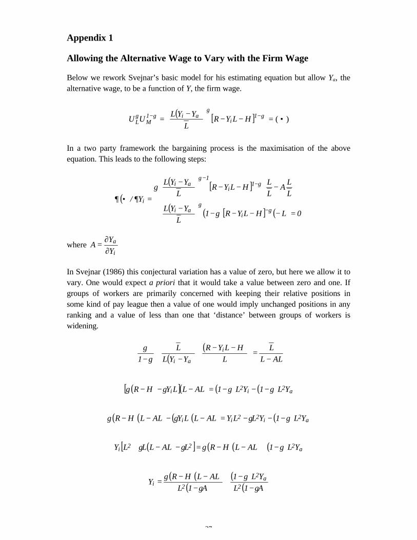
Finally, Table 9 reports the results of estimation in first differences. The results here,by contrast with those reported above, are somewhat inconclusive. The HSP andWinsorising results indicate that workers in state-owned firms are taking a smallershare of the surplus than when estimated in levels – 14 per cent (Winsorising) or 16per cent (HSP). All but one of the ownership coefficients are insignificant, meaning weare unable to detect significant differences between the process of wage determinationin state firms and private or mixed firms. Finally, even the alternative wage, highlysignificant in all the previous estimations, is insignificant in our first-differences results.A possible explanation for these poor results, and for the insignificant coefficient onthe alternative wage in particular, is that measurement error is overwhelming the truechanges in the underlying variables.
6. Conclusions
In this paper we have analysed the relationship of ownership form to wagedetermination in Russia using a firm-level dataset that includes several thousandindustrial and construction firms from four representative regions of Russia. Ourempirical results can be summarised as follows.
We find that wage determination is indeed related to ownership form in Russia.Workers in state-owned firms take a larger share of their firm’s surplus than workers inprivate (privatised) firms. Interestingly, the share of the surplus taken by workers infirms with mixed state/private ownership is similar to that in fully private firms. Theseresults can be interpreted as suggesting that corporate governance (wage setting) ismore disciplined in private firms, and that partial privatisation is enough to generatethis improved wage discipline.
We also find that our results are highly sensitive to the treatment of outliers in the data,and the conclusions above must be taken with this caveat in mind. There is no easyanswer to this problem – remarkably, we found that several outlier detection androbust estimation techniques were unable to detect a single gross outlier, theinclusion/exclusion of which had a huge impact on our estimation results. Our strategywas to use a wide range of such techniques, report the results of all of them, and theninvestigate further using a subset of these techniques that generated results that werereasonable on both statistical grounds and on the grounds of consistency with priorexpectations based on theory and other evidence. We would recommend that otherresearchers do the same when employing problematic data – as data from transitioncountries often are.

18
References
Ashenfelter, Orley and James N. Brown (1986), ‘Testing the Efficiency of EmploymentJournal of Political Economy, 94(3), pt.2, pp. 40–80.
Barnett, V. and T. Lewis (1994), Outliers in Statistical Data, New York: John Wiley& Sons, Inc.
Behnken, D. A. and N. R. Draper (1972), ‘Residuals and their Variance Pattern’,Technometrics, 14, pp. 101–11.
Belsley, D., E. Kuh and R. E. Welsch (1980), Regression Diagnostics, New York:John Wiley & Sons, Inc.
Bollen, K. A. and R. W. Jackman (1990), ‘Regression Diagnostics: An ExpositoryTreatment of Outliers and Influential Cases’, In: Fox, J. and J. S. Long (eds.),Modern Methods of Data Analysis, Newbury Park: Sage Publications,pp. 257-91.
Booth, A. L. (1995), The Economics of the Trade Union, Cambridge, MA: CambridgeUniversity Press.
Brown, D. (1996), ‘Excess Labour and Managerial Shortage: Findings From a Surveyin St. Petersburg’, Europe Asia Studies, 48(5), pp. 811–35.
Chatterjee, S. and A. S. Hadi (1988), Sensitivity Analysis in Linear Regression, NewYork: John Wiley & Sons, Inc.
Cook, R. D. (1977), ‘Detection of Influential Observations in Linear Regression’,Technometrics, 19, pp. 15–18.
Cook, R. D. and S. Weisberg (1982), Residuals and Influence in Regression, NewYork: Chapman and Hall.
Currie, J. (1991), ‘Employment Determination in a Unionised Public-Sector LabourMarket: The Case of Ontario’s School Teachers’, Journal of Labour Economics,9(1), pp. 45–66.
Draper, N. R. and H. Smith (1996), Applied Regression Analysis, New York: JohnWiley & Sons, Inc.
Gentleman, J. F. and M. B. Wilk (1975), ‘Detecting Outliers II: Supplementing theBiometrics, 31, pp. 387–410.
Greene, W. H. (1993), Econometric Analysis, 2nd. Edition, Prentice-Hall InternationalInc., p. 288.
Grubs, F. E. (1969), ‘Procedures for detecting outlying observations’, Technometrics,11, pp. 1–21.
Hadi, A. S. and J. S. Simonoff (1993), ‘Procedures for the Identification of MultipleJournal of the American Statistical Association,
88(424), pp. 1,265–72.Layard, R. and S. Nickell (1990), ‘Is Unemployment Lower if Unions Bargain Over
Quarterly Journal of Economics, August, 105(3), pp. 773–87.Lehmann, H., J. Wadsworth and A. Acquisti (1998), ‘Grime and Punishment: Job
Insecurity and Wage Arrears in the Russian Federation’, William DavidsonInstitute Working Paper Series, Ann Arbor, Michigan.
19
Lockwood, B. and A. Manning (1989), ‘Dynamic Wage-Employment Bargaining withEconomic Journal, 99, pp. 1,143–58.
MaCurdy, T. E. and J. H. Pencavel (1986), ‘Testing Between Competing Models ofWage and Employment Determination in Unionised Markets’, Journal ofPolitical Economy, 94(3), pt 2, pp. S3–S39.
McDonald, I. and R Solow (1981), ‘Wage Bargaining and Employment’, AmericanEconomic Review’, 71(5), pp. 896–908.
Prasnikar, J., J. Svejnar, M. Dubravko and V. Prasnikar (1994), ‘Behaviour ofParticipatory Firms in Yugoslavia: Lessons for Transforming Economies’, TheReview of Economics and Statistics, 76(4), pp. 728–41.
Prasnikar, J., J. Svejnar and K. Matjaz (1997), ‘Investment and Wages in the SlovenianFirms During the Transition’, working paper, draft copy.
Reiss, P. C. (1990), ‘Detecting Multiple Outliers with an Application to R&DJournal of Econometrics, 43, pp. 293–315.
Rousseeuw, P. J. and A. M. Leeroy (1987), ‘Robust Regression and OutlierDetection’, New York: John Wiley & Sons, Inc.
Standing, G. (1996), ‘Russian Unemployment and Enterprise Restructuring –Reviving Dead Souls’, London: Macmillian Press, Chapter 5: The Paradox ofWage Flexibility.
Svejnar, J. (1986), ‘Bargaining Power, Fear of Disagreement, and Wage Settlements:Theory and Evidence from U.S. Industry’, Econometrica, 54(5), pp. 1,055–78.
Thomas, R. L. (1997), Modern Econometrics – An Introduction, Harlow: AddisonWesley Longman.
Welsch, R. E. and E. Kuh (1977), Technical Report 923-77: Linear RegressionDiagnostics, Cambridge, MA: Sloan School of Management, MassachusettsInstitute of Technology.

21
TablesTable 1: Summary Statistics by Ownership Category
1996 obs. Total Sample Mean (St.Dev)
obs. State Firms Mean (St.Dev)
obs. Privatised FirmsMean (St. Dev)
obs. Mixed Firms Mean(St. Dev)
Employment 2331 612.81 (2497.06) 705 324.75 (1018.85) 605 508.01 (1099.96) 1021 873.83 (3560.68)Average Wage 2331 10.52 (8.12) 705 9.19 (6.06) 605 11.82 (10.97) 1021 10.66 (7.19)Alternative wage 2331 11.84 (4.68) 705 11.97 (4.56) 605 12.01 (4.42) 1021 11.65 (4.90)Output 2201 59866.98 (424332.6) 664 18821.24 (81146.91) 564 44635.67 (203249 1) 973 96706.47
(613576.3)Output per Employee 2201 61.14 (105.69) 664 40.31 (49.47) 564 69.09 (82.86) 973 70.76 (138.60)Profit 2331 8766.08 (130374.4) 705 4317.56 (39129.45) 605 4252.32 (12240.87) 1021 14512.44
(193967.2)Profit per Employee 2331 64.04 (1928.052) 705 23.99 (487.17) 605 8.57 (16.35) 1021 124.57 (2884.63)
1997 obs. Total Sample Mean (St.Dev)
obs. State Firms Mean (St.Dev)
obs. Privatised FirmsMean (St. Dev)
obs. Mixed Firms Mean(St. Dev)
Employment 2355 560.10 (2319.89) 707 299.41 (944.07) 615 463.50 (1024.93) 1033 796.03 (3306.60)Average Wage 2355 12.50 (8.56) 707 11.06 (7.62) 615 13.39 (8.64) 1033 12.96 (8.99)Alternative wage 2355 14.47 (5.51) 707 14.67 (5.39) 615 14.61 (5.22) 1033 14.24 (5.74)Output 2226 61045.46 (428830.1) 661 20822.06 (98035.58) 577 48959.52 (227310.1) 988 95014.34
(612904.2)Output per Employee 2226 68.16 (109.04) 661 45.48 957.32) 577 79.71 (119.91) 988 76.59 (125.38)Profit 2355 11957 (232431.7) 707 4549.91 (48360.52) 615 5066.77 (27904.09) 1033 21128.63 (347875)Profit per Employee 2355 42.29 (864.89) 707 27.56 (624.83) 615 9.31 (41.12) 1033 72.01 (1198.54)

22
Table 2: Summary Statistics by Industry Category
obs. Industry Mean 1996(St. Dev)
obs. Industry Mean 1997(St. Dev)
obs. Construction Mean1996
(St. Dev)
obs. Construction Mean1997
(St. Dev)Employment 1768 712.26 (2817.66) 1789 651.49 (2618.76) 562 300.52 (872.73) 565 271.12 (781.90)Average Wage 1768 9.74 (6.36) 1789 11.71 (7.75) 562 12.97 (11.76) 565 15.02 (10.35)Alternative wage 1768 10.82 (3.97) 1789 13.29 (4.91) 562 15.06 (5.26) 565 18.20 (5.63)Output 1730 71120.83 (476957.8) 1751 72516.11 (482223.9) 498 17515.4 (59928.69) 500 17807.37 (48028.62)Output per Employee 1730 62.39 (114.18) 1751 67.36 (101.29) 498 53.45 (65.06) 500 67.53 (131.41)Profit 1768 7000.49 (93495.98) 1789 12223.78 (255011.7) 562 14142.3 (207377.9) 565 10883.02 (138896.1)Profit per Employee 1768 6.54 (18.47) 1789 5.98 (29.59) 562 244.39 (3923.67) 565 156.59 (1761.20)

23
Table 3: Regression Diagnostics and Robust Estimation for 1997
FullSample
Hadi&
Simonoff
Dffits Cook’sDistance
Welsch’sDistance
Covratio NonLinearLeast
Squares
MedianLeast
Squares
RLS RobustRegression
Winsor MinusOne
valad 97 0.001 0.339 0.001 0.277 0.001 0.248 0.001 0.001 0.001 0.346 0.340 0.270(0.000)* (0.012)** (0.000)** (0.013)** (0.000)* (0.013)** (0.000)* (0.000)** (0.000)* (0.010)** (0.012)** (0.015)**
private*valad97 0.071 –0.045 0.047 –0.095 0.055 –0.042 0.070 0.202 0.215 –0.111 –0.073 –0.198(0.007)** (0.016)** (0.006)** (0.017)** (0.007)** (0.016)** (0.007)** (0.005)** (0.010)** (0.013)** (0.015)** (0.016)**
mixed*valad97 –0.001 –0.061 –0.001 –0.263 –0.001 –0.235 –0.001 0.000 –0.001 –0.346 –0.087 –0.270(0.000) (0.014)** (0.000)** (0.013)** (0.000)** (0.013)** (0.000) (0.000)** (0.000) (0.010)** (0.014)** (0.015)**
Private 0.908 0.167 0.770 0.303 0.783 0.274 1.049 0.498 0.374 0.196 0.143 0.857(0.242)** (0.146) (0.203)** (0.177) (0.216)** (0.169) (0.233)** (0.179)** (0.217) (0.161) (0.142) (0.227)**
Mixed 1.249 0.381 1.064 0.947 1.021 0.819 1.275 1.045 1.129 0.596 0.420 1.233(0.205)** (0.124)** (0.171)** (0.149)** (0.182)** (0.143)** (0.205)** (0.152)** (0.182)** (0.135)** (0.120)** (0.192)**
alt wage97 0.680 0.576 0.562 0.614 0.585 0.584 0.720 0.682 0.623 0.573 0.538 0.665(0.039)** (0.027)** (0.033)** (0.032)** (0.035)** (0.029)** (0.027)** (0.028)** (0.034)** (0.026)** (0.027)** (0.036)**
Moscow –0.308 –0.106 –0.359 –0.378 –0.260 –0.446 –0.308 –0.472 –0.300 –0.254 –0.182 –0.200(0.254) (0.156) (0.213) (0.186)* (0.227) (0.178)* (0.254) (0.186)* (0.216) (0.168) (0.152) (0.238)
Chuvashia –1.026 –1.036 –1.391 –1.198 –1.319 –1.191 –1.026 –0.998 –1.150 –1.060 –1.108 –1.021(0.293)** (0.176)** (0.244)** (0.211)** (0.260)** (0.204)** (0.293)** (0.214)** (0.248)** (0.194)** (0.171)** (0.274)**
Krasnoyarsk 0.118 1.056 –0.290 0.302 –0.149 0.286 0.118 –0.081 –0.009 0.548 0.938 0.620(0.314) (0.189)** (0.262) (0.227) (0.279) (0.219) (0.314) (0.230) (0.267) (0.209)** (0.181)** (0.295)*
Construction –0.119 0.169 –0.326 –0.226 –0.163 –0.136 –0.119 0.049 –0.172 0.120 0.086 0.201(0.235) (0.146) (0.198) (0.175) (0.210) (0.167) (0.235) (0.172) (0.200) (0.156) (0.141) (0.220)
Constant 0.999 1.652 1.971 1.575 1.834 1.800 0.999 0.679 1.610 1.686 1.968 0.950(0.364)** (0.240)** (0.308)** (0.283)** (0.328)** (0.265)** (0.364)** (0.266)* (0.310)** (0.241)** (0.234)** (0.340)**
N 2354 2256 2294 2282 2326 2254 2354 2354 2347 2352 2354 2353R2 0.29 0.66 0.27 0.47 0.27 0.48 0.29 0.211 0.38 n.a. 0.66 0.37Outliers 0 98 60 72 28 100 0 0 7 2 0 1
Notes: ** significant at the 1 per cent level; * significant at the 5 per cent level; 1Refers to a pseudo R2.
24
Table 4: Gross Outlier and Rest of Sample Compared
Full Sample Less Gross Outlier, i.e., 2,353 observationsGross Outlier Mean Standard
DeviationMin Max
Wage 17.341 7.206 4.933 0. 029 58.393Alternative wage 14.380 8.343 3.176 2.335 23.916Profit 507694.7 6651.679 133706 –233775.2 6072081Profit per worker 9579.145 20.238 458.465 –203.189 17585.85Value added perworker
9582.105 19.102 458.570 –215.458 17591.6
Employment 53 560.413 2320.851 1 73930
Table 5: Estimation using OLS 1996
1996 Full Sample Hadi &Simonoff
Winsorising Minus One
Valad 96 0.001 0.312 0.320 0.115(0.0004)* (0.011)** (0.011)** (0.009)**
Private*valad96 0.336 –0.069 –0.076 0.222(0.012)** (0.015)** (0.015)** (0.015)**
Mixed*valad96 –0.001 –0.055 –0.076 –0.115(0.0004) (0.014)** (0.013)** (0.009)**
Private –0.159 0.321 0.279 –0.058(0.246) (0.144)* (0.137)* (0.239)
Mixed 1.096 0.498 0.395 1.207(0.203)** (0.121)** (0.114)** (0.197)**
alt wage96 0.602 0.482 0.443 0.595(0.039)** (0.027)** (0.024)** (0.038)**
Constant 1.571 2.053 2.435 1.462(0.347)** (0.224)** (0.203)** (0.337)**
N 2330 2235 2330 2329R2 0.41 0.63 0.65 0.45
Notes: **significant at 1 per cent level, * 5 per cent level.

25
Table 6: Estimation using OLS 1997
1997 Full Sample Hadi &Simonoff
Winsorising Minus One
valad 97 0.001 0.339 0.340 0.270(0.0004)* (0.012)** (0.012)** (0.015)**
private*valad97 0.071 –0.045 –0.073 –0.198(0.007)** (0.016)** (0.015)** (0.016)**
mixed*valad97 –0.001 –0.061 –0.087 –0.270(0.0004) (0.014)** (0.014)** (0.015)**
Private 0.908 0.167 0.143 0.857(0.242)** (0.146) (0.142) (0.227)**
Mixed 1.249 0.381 0.420 1.233(0.205)** (0.124)** (0.120)** (0.192)**
alt wage97 0.680 0.576 0.538 0.665(0.039)** (0.027)** (0.027)** (0.036)**
constant 0.999 1.652 1.975 0.950(0.364)** (0.240)** (0.234)** (0.340)**
N 2354 2255 2354 2353R2 0.29 0.66 0.66 0.37
Table 7: Estimation using instrumental variables, 1996
1996 Full Sample Hadi &Simonoff
Winsorising Minus One
valad 96 0.008 0.313 0.151 0.120(0.005) (2.013) (0.072)* (0.083)
private*valad96 0.314 0.123 0.148 0.183(0.168) (1.496) (0.141) (0.183)
mixed*valad96 –0.007 3.481 0.130 –0.119(0.005) (34.792) (0.146) (0.083)
private 0.095 0.139 0.007 0.183(0.969) (4.120) (0.485) (0.911)
mixed 1.275 –7.757 0.174 1.310(0.244)** (84.714) (0.388) (0.236)**
alt wage96 0.607 –0.775 0.458 0.624(0.054)** (13.489) (0.059)** (0.048)**
constant 1.232 7.918 2.359 1.019(0.452)** (64.018) (0.409)** (0.427)*
N 2022 1938 2022 2021R2 0.36 . 0.62 0.45
Note: A full stop in the R2 box indicates that the calculated R2 was negative and hence is not reported.
26
Table 8: Estimation using instrumental variables, 1997
1997 Full Sample Hadi &Simonoff
Winsorising Minus One
valad 97 0.001 0.429 0.388 0.349(0.0004)* (0.025)** (0.014)** (0.031)**
private*valad97 0.226 –0.096 –0.100 –0.122(0.016)** (0.029)** (0.019)** (0.034)**
mixed*valad97 0.000 –0.120 –0.097 –0.349(0.001) (0.027)** (0.017)** (0.031)**
private 0.115 0.012 0.059 0.051(0.278) (0.152) (0.145) (0.265)
mixed 1.216 0.267 0.313 1.198(0.227)** (0.129)* (0.122)* (0.216)**
alt wage97 0.613 0.555 0.510 0.594(0.043)** (0.028)** (0.027)** (0.041)**
constant 1.572 1.770 2.132 1.505(0.407)** (0.247)** (0.236)** (0.387)**
N 2322 2226 2322 2321R2 0.13 0.65 0.66 0.21
Table 9: Estimation in First Differences, 1996–97
Full Sample Hadi &Simonoff
Winsorising Minus One
diff valad 96 0.002 0.157 0.140 0.021(0.003) (0.013)** (0.013)** (0.009)*
private*diff 0.068 –0.013 0.015 0.048valad96 (0.007)** (0.017) (0.017) (0.011)**mixed*diff –0.002 –0.031 –0.033 –0.021valad96 (0.003) (0.016) (0.015)* (0.009)*private –0.254 –0.078 –0.001 –0.282
(0.193) (0.097) (0.085) (0.193)mixed 0.107 –0.027 0.050 0.081
(0.164) (0.083) (0.072) (0.165)diff alt wage96 0.034 0.026 0.112 0.021
(0.153) (0.078) (0.074) (0.153)constant 0.257 0.322 0.271 0.282
(0.221) (0.111)** (0.097)** (0.221)N 2323 2218 2323 2322R2 0.07 0.20 0.20 0.07
27
Appendix 1
Allowing the Alternative Wage to Vary with the Firm Wage
Below we rework Svejnar’s basic model for his estimating equation but allow Ya, thealternative wage, to be a function of Y, the firm wage.
( ) [ ] γγ
γγ −− −−
−
= 1i
ai1ML HLYR
L
YYLUU = ( • )
In a two party framework the bargaining process is the maximisation of the aboveequation. This leads to the following steps:
( ) =• iY/ ∂∂
( ) [ ]
( ) ( )[ ] ( ) 0LHLYR1L
YYL
L
LA
L
LHLYR
L
YYL
iai
1i
1ai
=−−−−
−
+
−−−
−
−
−−
γγ
γγ
γ
γ
where i
a
Y
YA
∂∂
=
In Svejnar (1986) this conjectural variation has a value of zero, but here we allow it tovary. One would expect a priori that it would take a value between zero and one. Ifgroups of workers are primarily concerned with keeping their relative positions insome kind of pay league then a value of one would imply unchanged positions in anyranking and a value of less than one that ‘distance’ between groups of workers iswidening.
( )( )
ALL
L
L
HLYR
YYL
L
1i
ai −=
−−
−
− γγ
( )[ ]( ) ( ) ( ) a2i2i YL1YL1ALLLYHR γγγγ −−−=−−−
( )( ) ( )( ) ( ) a2i22ii YL1YLLYALLLYALLHR γγγγ −−−=−−−−
( )[ ] ( )( ) ( ) a222i YL1ALLHRLALLLLY γγγγ −+−−=−−+
( )( )( )
( )( )A1L
YL1
A1L
ALLHRY
2a2
2iγ
γγ
γ−
−+
−−−
=
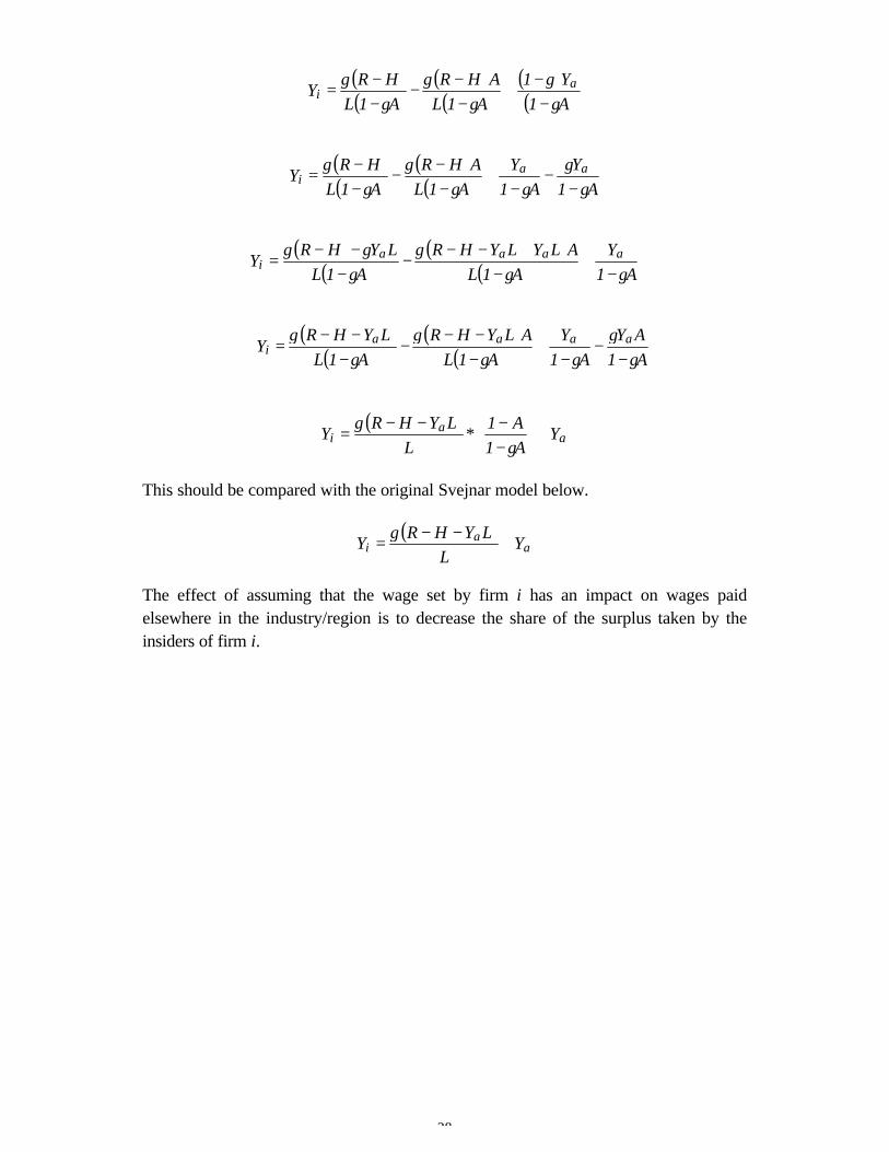
28
( )( )
( )( )
( )( )A1
Y1
A1L
AHR
A1L
HRY a
iγ
γγ
γγ
γ−
−+
−−
−−−
=
( )( )
( )( ) A1
Y
A1
Y
A1L
AHR
A1L
HRY aa
iγ
γγγ
γγ
γ−
−−
+−−
−−−
=
( )( )
( )( ) A1
Y
A1L
ALYLYHR
A1L
LYHRY aaaa
iγγ
γγ
γγ−
+−
+−−−
−−−
=
( )
( )( )
( ) A1
AY
A1
Y
A1L
ALYHR
A1L
LYHRY aaaa
iγ
γγγ
γγ
γ−
−−
+−−−
−−
−−=
( )a
ai Y
A1
A1
L
LYHRY +
−−
∗−−
=γ
γ
This should be compared with the original Svejnar model below.
( )a
ai Y
L
LYHRY +
−−=
γ
The effect of assuming that the wage set by firm i has an impact on wages paidelsewhere in the industry/region is to decrease the share of the surplus taken by theinsiders of firm i.
29
Appendix 2
Residual Classification and Diagnostic/Robust Techniques
Standardisation of the Residuals
In the brief descriptions that follow there are several measures of residuals used. AsGreene (1993) points out, if one wishes to identify which residuals are significantlylarge they should be standardised by dividing by the appropriate standard error for thatparticular residual.
Studentisation refers to the division of a scale-dependent statistic by a scale estimatethat results in a statistic which is free of the nuisance scale parameters.13 A furtherdistinction is between internal and external studentisation. In the former, the scalestatistic and the scale estimate are derived from the same data; in the latter they areindependent but the necessary information for the construction of the residual comesfrom the fitting of the model using all the data to hand. For predicted residuals,calculations are based on a fit that has taken place without including the ith observation.The same division between internal and external can then be made.
The Standardised Residual
One residual used in outlier identification is the standardised residual. (This is the termthe Stata Corporation use.) Hadi and Simonoff (1993) refer to this as the ‘internallystudentised residual’ and Cook and Weisberg (1982), while acknowledging it as aninternally studentised residual when referring to (1.1), simply adopt the term‘studentised residual’.) It is defined as:
( )iih1sie
ie−
= (A2.1)
hii represents the ith diagonal element of the hat matrix H; s is the variance from thesample residuals and ei is the ordinary residual.
Studentised Residual
A second residual used is the studentised residual. (This is what Hadi and Simonoffrefer to as the externally studentised residual.) It is defined as:
( )ii
ii
h1s
er
)i( −= (A2.2)
The (i) here refers to the fact that the standard error is calculated without using the ith
observation. Hence the residual is independent from the standard error. s(i) is obtainedfrom:
13 Cook and Weisberg (op. cit., p. 18).
30
( )( ) ( )
−−
−−=
−−−−−
=
1kn
ekns
1kn
h1eskns
2i2
ii2i
22i
(A2.3)
where n is the number of observations and k the number of explanatory variables.
Predicted Residuals
The ith predicted residual is found by estimating the given model without the ith
observation and then using the least squares estimator of β to find the residual, i.e.,
( ) ( ) ( ) n 2,..., 1,i ˆe iTiii =−= βxy (A2.4)
The predicted error can then be divided by the standard error of the prediction toobtain:
( )iψ ( )
( ) ( ) ( )( )[ ] 21i
1iiii
i
xXXx1s
e
−+=
TT(A2.5)
where ix is a row vector of explanatory variables on the ith observation and ( )iX is
obtained from the matrix X by deleting the ith row Tix . Moreover, the above scaled
predicted residual is equal to the externally studentised residual, i.e., r(i). As mentionedin the main body of the text the coefficient on a dummy variable that has a one for theith observation and zeros elsewhere will equal the predicted residual and the t statistic isequal to the externally studentised residual.
We can link the internally and externally studentised residuals with the predictedresiduals. From the mean shift outlier model we know that:
( ) =ieii
i
h1
e
−(A2.6)
where e(i) is the predicted residual, ei the ordinary residual. The externally studentisedresidual is given by:
( )ii
ii
h1
er
)i(s −= (A2.7)
(A2.6) can be rearranged to give:
( ) iiiii h1sre −×= (A2.8)
Substituting and rearranging gives:
31
( )( )
( ) iii
ii
h1s
er
−= (A2.9)
If we require the standard error with the ith observation then we have
( )( )
ii
ii
h1s
ee
−= (A2.10)
where ( )ie is the internally studentised residual or the standardised residual.
Formulae for Outlier Detection
The basic formulae used in each of the outlier detection methods are given below alongwith possible connections between the various methods. As will be seen, they make usemainly of the studentised and the standardised residuals.
1) DFFITS (Welsch and Kuh, 1977 and Belsley, Kuh and Welsch, 1980)This measures the difference between the fitted value y of y that results from
dropping a particular observation. If ( )iy is the fitted value of y once the ith
observation is deleted then the quantity ( )( )iyy − divided by the scaling factor ( )iiish ,
where ( )is is the estimator of 2σ from a regression with the ith observation omitted is
called DFFITS. It has been shown by Belsley et al.(1980) that:
( )iiiiii h1hrDFFITS −= (A2.11)
where ri are the studentised residuals. It should be noted that Belsley, Kuh and Welschdo not actually suggest dropping outliers even if upon examination they prove to beanomalous. Rather they suggest a bounded influence estimation where (to simplify)Welsch (1980) suggests that the regression is run; DFFITS is calculated and on thebasis of the absolute value of DFFITS weights are attached by the following rule:
Minimize ( )∑ − 2iii xyw β , where 1wi = if 34.0DFFITS ≤ or
DFFITS
34.0wi = if
DFFITS >0.34. If we had pursued this approached then this would have placed this in
the robust category since it is clearly an attempt to accommodate outliers andinfluential observations. In our study we merely adopt the suggested cutoff value
2√(k/n).
2) Cook’s Distance (Cook, 1977)Cook’s Distance is given by:
( )( )
i22
2i
2i2
2ii
i DFFITSs
s
k
1
h1ks
ehD =
−= (A2.12)
32
where k is the number of variables including the constant in the regression, s is the rootmean square error of the regression and s(i) is the root mean square error of theregression with the ith observation omitted.
3) Welsch’s DistanceWelsch’s Distance is given by:
( )( ) ii
iii
iiii
h1
1nDFFITS
h1
1nhrW
−−
=−
−= (A2.13)
Values of Cook’s distance greater than 4/n should be examined (Bollen and Jackman,
1990). Following similar logic, the cut-off for Welsch’s Distance is approximately 3√k(Chatterjee and Hadi, 1988).
4) Covratio
ii
ki
h1
1
1kn
ekncovratio
−
−−−−
= (A2.14)
This measure is the ratio of the determinants of the covariance matrix, with andwithout the ith observation. Belsley, Kuh and Welsch (1980) suggest that observationsfor which
n
k31covratioi ≥− (A2.15)
should be investigated further. In the calculation of outliers using the above proceduresthe recommended cut-off points were used.
5) Hadi Process (Hadi and Simonoff, 1993)The Hadi and Simonoff procedure (HSP) firstly involves identifying an initial cleansubset M, initially of size h = integer part of (n + k –1)/2. Hadi and Simonoff (1993)propose two methods of identifying the initial subset. With the first method, M1, thedataset is divided into a basic subset that contains the first k + 1 observations and anon-basic subset that contains the remaining (n – k – 1) observations. This is done afterfitting a regression model to the whole dataset and then ordering the n observationsaccording to some regression diagnostic, say, the absolute value of the adjusted
residual, which is defined as iih1
ieie
−= . Run a regression on the subset B, i.e., the
basic subset. Compute iih1
ieie
−= if Bi ∈ and
iih1ie
ie+
= if Bi ∉ and
arrange the observations in ascending order. The size of the basic subset, s, is increasedby one observation to s + 1. Repeat the above. When the size of the basic subset equalsh substitute the first h observations for M and go to step 2 of their main algorithm (seebelow). M2, the second method is left for the cited reference. M1 is described in detailhere since Hadi and Simonoff found that it was more powerful in the presence of high
33
leverage outliers compared to M2 but there was little difference in the presence of lowleverage outliers.
In the second step of their algorithm the following is calculated:
( ) ix1XXix1ˆ
ˆixi
id−′′−
′−=
MMM
My
σ
β , if Bi ∈ and (A2.16)
( ) ix1XXix1ˆ
ˆixi
id−′′+
′−=
MMM
My
σ
β if Bi ∉ (A2.17)
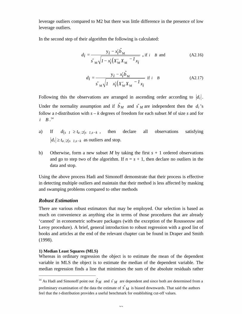
Following this the observations are arranged in ascending order according to id .
Under the normality assumption and if Mβ and Mσ are independent then the id ’s
follow a t-distribution with s – k degrees of freedom for each subset M of size s and forBi ∉ .14
a) If ( ) ( )ks,1s21s td −++ ≥ α , then declare all observations satisfying
( )ks,1s2i td −+≥ α as outliers and stop.
b) Otherwise, form a new subset M by taking the first s + 1 ordered observationsand go to step two of the algorithm. If n = s + 1, then declare no outliers in thedata and stop.
Using the above process Hadi and Simonoff demonstrate that their process is effectivein detecting multiple outliers and maintain that their method is less affected by maskingand swamping problems compared to other methods
Robust Estimation
There are various robust estimators that may be employed. Our selection is based asmuch on convenience as anything else in terms of those procedures that are already‘canned’ in econometric software packages (with the exception of the Rousseeuw andLeroy procedure). A brief, general introduction to robust regression with a good list ofbooks and articles at the end of the relevant chapter can be found in Draper and Smith(1998).
1) Median Least Squares (MLS)Whereas in ordinary regression the object is to estimate the mean of the dependentvariable in MLS the object is to estimate the median of the dependent variable. Themedian regression finds a line that minimises the sum of the absolute residuals rather 14 As Hadi and Simonoff point out Mβ and Mσ are dependent and since both are determined from a
preliminary examination of the data the estimate of Mσ is biased downwards. That said the authorsfeel that the t-distribution provides a useful benchmark for establishing cut-off values.

34
than the sum of the squares of the residuals as in OLS, i.e., minimise, with respect tothe elements of β .
( )βTiiYMedian x−
It is usual to see a pseudo R2 reported with MLS. This is calculated as
1 – (the sum of the absolute deviations about the predicted Y)/ (the raw sum ofabsolute deviations about the unconditional median)A more rigorous procedure advocated by Rousseeuw and Leroy (1987) is explainedbelow. While MLS results are reported, results based on this procedure are alsoreported below.
2) Reweighted Least Squares (Rousseeuw and Leroy Procedure)The following procedure does not appear explicitly in full within the book byRousseeuw and Leroy (1987) but is taken from various parts of the book.
Step 1. Run MLS.15
Step 2. Calculate a preliminary scale estimate S0
2i
i0 r med
pn
514826.1s
−
+=
where ri is the residual, n the sample size and p the number of explanatory variables.
Step 3. Calculate the standardised residuals 0is
r .
Step 4. Determine the weights iw for the ith observation based on
otherwise 0 or 5.2s
r if 1w 0ii ≤
= .
Step 5. Calculate the scale estimate for LMS regression using
∑
∑
=
=
−=
n
1ii
n
1i
2ii
*
pw
rw
σ .
Step 6. Standardise the residuals using σ*. If 5.2r*
i >σ investigate the observation as
a possible outlier.
15 Strictly speaking the dataset should be standardised before the above procedure is carried out. Thismakes the variables dimensionless and so helps avoid numerical inaccuracies caused by different unitsof measurement. Rousseeuw and Leroy recommend that the median of the jth variable is subtractedfrom the ith observation on the jth variable. This in turn is divided by the median of the absolute
deviations from the median multiplied by the correction factor ( ) 4826.175.0
11 ≈−φ . After MLS
the results, of course, have to be transformed back. The Stata command qreg with its default setting isMLS but qreg does not transform the variables to be dimensionless (personal e-mail from Stata’stechnical support 22/4/99). Whether by transforming the data as suggested by Rousseeuw and Leeroywould have made a great deal of difference to the final results reported is open to question.

35
Step 7. Carry out reweighted least squares (RLS). In effect OLS except on the reduceddataset formed on the basis of deleting observations deemed outliers in step 6 above.
3) WinsorisingThis is similar to the so-called α-trimmed mean, which is simply the mean of the
sample after the proportion α of the largest and smallest observations have beendeleted from the data. However, the Winsorised mean, rather than discarding the
proportion α, ‘accumulates’ them at either end of the truncation point. In theregressions run using the Winsorising technique the largest and smallest 5 per cent ofobservations were ‘Winsorised’.
4) Non Linear Least SquaresIf transforming variables by taking natural logarithms can lessen the impact of outliersit might be worth exploring whether estimating the model by non-linear least squaresassuming a k shifted log normal errors might lessen the impact of influentialobservations within the dataset. The specification is as follows.
( ) [ ]( ) i210 kwage ealternativ97valadlnkwageln νβββ +−++=−
In running the regression k is given a value of zero, which is the case of proportionerrors since the standard error of the response variable, here the log of the firm wage,is proportional to its expected value.
5) Robust RegressionIn this procedure implemented by the statistical package Stata, Cook’s Distance, D, isfirst calculated (see above) and then any observations from the regression which have aD larger than 1 are excluded. An iterative procedure then follows where weights arecalculated on the basis of the residuals and then the regression is repeated. The processstops when the maximum change in weights drops below a certain level. There are twoweight functions used: 1) Huber weights and 2) biweights. Both are used since Huberweights have problems dealing with severe outliers while biweights sometimes fail toconverge or have multiple solutions.16
A. Huber weights
The ith scaled residual is calculated from s
eu i
i = where ei is the ordinary residual and
6745.0
Ms = is the residual scale estimate and ( )( )ii emedemedM −= is the median
absolute deviation from the median residual. The case weights are given by
hii cuif 1w ≤= if not then ihi ucw = where ch = 1.345. So downweighting starts
when the absolute value of a residual exceeds (1.345/ 0.6745)M which is about 2M.
16 This brief summary is taken from the Stata Reference Manual, volume 3, Release 4, p. 135.

36
B. BiweightsAll observations with non-zero residuals receive some downweighting using thefollowing smoothly decreasing biweight function.
( )[ ] hi22
bii cuifcu1w ≤−= or 0 otherwise
where cb = 4.685 (tuning value)/7. The tuning value can be altered with higher tuningconstants producing milder downweighting and lower ones giving more drasticdownweighting to the residuals. In the robust regression results reported the defaultsetting of 7 was used.